The Degrees-of-Freedom in Monostatic ISAC Channels: NLoS Exploitation vs. Reduction

Abstract

The degrees of freedom (DoFs) attained in monostatic integrated sensing and communications (ISAC) are analyzed. Specifically, monostatic sensing aims for extracting target-orientation information from the line of sight (LoS) channel between the transmitter and the target, since the Non-LoS (NLoS) paths only contain clutter or interference. By contrast, in wireless communications, typically, both the LoS and NLoS paths are exploited for achieving diversity or multiplexing gains. Hence, we shed light on the NLoS exploitation vs. reduction tradeoffs in a monostatic ISAC scenario. In particular, we optimize the transmit power of each signal path to maximize the communication rate, while guaranteeing the sensing performance for the target. The non-convex problem formulated is firstly solved in closed form for a single-NLoS-link scenario, then we harness the popular successive convex approximation (SCA) method for a general multiple-NLoS-link scenario. Our simulation results characterize the fundamental performance tradeoffs between sensing and communication, demonstrating that the available DoFs in the ISAC channel should be efficiently exploited in a way that is distinctly different from that of communication-only scenarios.

I Introduction

In the forthcoming 5G-Advanced and 6G wireless networks, radio sensing at the network level has been considered as a beneficial new feature in support of emerging applications such as vehicle-to-everything (V2X) communications, as well as smart city and unmanned aerial vehicle (UAV) networks [1]. In the meantime, given the imminent spectrum crunch of wireless communications, the radar bands can be harnessed as alternative spectral resources. Owing to the commonalities between sensing and communication (S$\&$C) in terms of hardware architecture and signal processing algorithms [2], Integrated Sensing and Communications (ISAC) constitutes a promising solution for embedding attractive radar sensing functionalities into the existing cellular infrastructure in a prompt and low-cost manner. Hence, it has received tremendous research attention in the recent years [3, 4, 5, 6, 7, 8].

Conventional radar systems are conceived solely for optimizing the sensing performance without addressing the communication functionality [9, 10, 11]. With the emerging integration of S$\&$C, both sensing-centric as well as communication-centric and joint designs are proposed for ISAC signal processing, which lead to flexible performance tradeoff between S$\&$C [2]. In this spirit, novel resource allocation and waveform design approaches were developed [12] for approaching the ISAC performance bounds, leading to attractive integration and coordination gains [3]. More recently, numerous design tradeoffs have been revealed [2], ranging from information theoretical tradeoffs to physical layer tradeoffs [4], and to cross-layer designs [5].

While the aforementioned contributions relied upon sophisticated techniques, they generally assume that the S$\&$C signals propagate over channels exhibiting similar statistical characteristics, even though in practical scenarios, things become more complex. Briefly, the presence of multiple paths can be exploited by the communication functionality. But not all the paths are useful for radar sensing [2]. Specifically, radar detection is typically more dependent on the direct line of sight (LoS) link between the radar transceiver and the target, since Non-LoS (NLoS) links typically contain unwanted clutter [11]. By contrast, wireless systems attain higher spatial degrees of freedom (DoFs) by exploiting both LoS and NLoS links. By noting this fundamental difference in S$\&$C propagation channels, it is of pivotal importance to design efficient resource allocation for exploiting the spatial DoFs inherent within the ISAC channels, which motivates our research.

Explicitly, we consider an ISAC base station (ISAC-BS) that supports a single communication user, which is also a target to be sensed. A typical example for such a scenario is the sensing-assisted vehicle-to-infrastructure (V2I) communication scenario, where a roadside unit (RSU) wishes to communicate with a vehicle, while simultaneously tracking its movement [3]. To be specific, we design a novel power allocation (PA) strategy for balancing the fundamental performance tradeoff between the S$\&$C spatial DoFs. We assume that there always exists a LoS link for target detection or tracking. Since unknown reflection coefficients may reduce the received signal energy to a level that does not allow reliable detection [9], the ISAC-BS estimates the reflection coefficient of each path first, and then judiciously share its total power across different paths through tailormade transmit beamforming (TBF). To gain deeper insights into the PA design, we first consider the special case, where there is only a single NLoS link in addition to its LoS counterpart, and derive the optimal PA scheme in closed form. Then, we extend it to a multiple-NLoS-link scenario and provide a sub-optimal solution based on the popular successive convex approximation (SCA) algorithm. Finally, our simulations characterize the performance tradeoff between S$\&$C, which indicates that both the S$\&$C performance can be simultaneously optimized by effectively exploiting all ISAC spatial DoFs.

II System Model

We consider the downlink (DL) of a ISAC system, where the ISAC-BS is equipped with $N_{T}$ transmit antennas (TAs) and $N_{R}$ receive antennas (RAs) as shown in Fig. 1. The ISAC-BS is serving a single-antenna user (which is also treated as a point-like target) for simultaneously supporting S$\&$C services. We assume that there are $K$ channel impulse response (CIP) paths between the ISAC-BS and the target, only one of which is the LoS link. Let $\mathcal{K}\triangleq\{0,1,\cdots,K-1\}$ denote the index set of the $K$ propagation paths. For notational convenience, we do not distinguish between scatterers within each propagation path and clutter sources. As a consequence, the ISAC-BS receives signal reflections from multiple paths, where only the LoS path contains the target information of interest, and the echoes from the NLoS paths are treated as clutter. In what follows, we elaborate on the S$\&$C signal models.

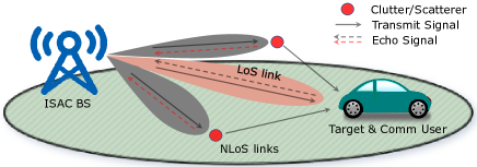
Figure 1: Illustration of the system considered.

II-A Sensing Signal Model

Let $\mathbf{s}=\left[s_{0},s_{1},\ldots,s_{K-1}\right]^{T}\in\mathbb{C}^{K\times 1}$ denote the ISAC transmit signal vector. Thus the echo signal arriving at the ISAC-BS receiver can be expressed as

$$\mathbf{y}_{r}= \underbrace{{\beta}_{0}\sqrt{p_{0}}\mathbf{b}\left(\theta_{0}\right)\mathbf{a}^{H}\left(\theta_{0}\right)\mathbf{F}\mathbf{s}}_{\text{Target/LoS link }}+\underbrace{\sum_{k=1}^{K-1}{\beta}_{k}\sqrt{p_{k}}\mathbf{b}\left(\theta_{k}\right)\mathbf{a}^{H}\left(\theta_{k}\right)\mathbf{F}\mathbf{s}}_{\text{Path-dependent Clutter/NLoS links}}$$

$$+\mathbf{z}_{r},$$ (1)

where $\beta_{0}$ and $\{\beta_{k}\}^{K-1}_{k=1}$ are independent and identically distributed (iid) reflection coefficients of the target and the $k$-th clutter/scatter source, while $p_{0}$ and $p_{k}$ represent the transmit power to the LoS and NLoS links, $\theta_{0}$ and $\theta_{k}$ are the angles of the target and the $k$-th path-dependent clutter source, $\mathbf{a}(\theta)=\frac{1}{\sqrt{N_{T}}}\left[1,e^{-j\pi\sin\theta},\cdots,e^{-j\pi\left(N_{T}-1\right)\sin\theta}\right]^{T}$ and $\mathbf{b}(\theta)=\frac{1}{\sqrt{N_{R}}}\left[1,e^{-j\pi\sin\theta},\cdots,e^{-j\pi\left(N_{R}-1\right)\sin\theta}\right]^{T}$ are the transmit and receive steering vectors, $\mathbf{F}=\left[\mathbf{f}_{0},\mathbf{f}_{1},\ldots,\mathbf{f}_{K-1}\right]\in\mathbb{C}^{N_{T}\times K}$ denotes the TBF matrix, and $\mathbf{z}_{\mathbf{r}}\in\mathbb{C}^{N_{R}\times 1}$ represents the additive white Gaussian noise (AWGN) with variance of $\sigma^{2}_{R}$, respectively.

Following the standard assumption of the radar literature [9, 10, 11], and given the fact that we focus our attention on power sharing among multiple paths, we assume that the angle for each path is perfectly predicted/tracked, thereby the beamforming gain $\mathbf{a}^{H}(\theta_{k})\mathbf{f}_{k}$ equals to 1 and $\mathbf{a}^{H}(\theta_{k})\mathbf{F}\mathbf{s}=s_{k}$. After receive beamforming (RBF) at the ISAC-BS receiver, the sensing signal output of the receiving filter is given by

$$y_{s} =\beta_{0}\sqrt{p_{0}}\mathbf{w}^{H}\mathbf{b}\left(\theta_{0}\right)s_{0}+\sum_{k=1}^{K-1}\beta_{k}\sqrt{p_{k}}\mathbf{w}^{H}\mathbf{b}\left(\theta_{k}\right)s_{k}+\mathbf{w}^{H}{\mathbf{z}_{r}},$$ (2)

where $\mathbf{w}$ is the RBF vector designed for maximizing the signal-to-clutter-plus-noise ratio (SCNR). As a consequence, the SCNR can be written as

$$\operatorname{SCNR} =\frac{\left|s_{0}\beta_{0}\sqrt{p_{0}}\mathbf{w}^{H}\mathbf{b}\left(\theta_{0}\right)\right|^{2}}{\sum_{k=1}^{K-1}\left|s_{k}\beta_{k}\sqrt{p_{k}}\mathbf{w}^{H}\mathbf{b}\left(\theta_{k}\right)\right|^{2}+\mathbf{w}^{H}\mathbf{w}\sigma_{R}^{2}}$$

$$=\frac{\frac{p_{0}\left|s_{0}\beta_{0}\right|^{2}}{\sigma_{R}^{2}}\left|\mathbf{w}^{H}\mathbf{b}\left(\theta_{0}\right)\right|^{2}}{\mathbf{w}^{H}\left(\boldsymbol{\Sigma}+\mathbf{I}_{N_{R}}\right)\mathbf{w}},$$ (3)

where $\boldsymbol{\Sigma}=\sum_{k=1}^{K-1}\frac{p_{k}\left|s_{k}\beta_{k}\right|^{2}}{\sigma_{R}^{2}}\mathbf{b}\left(\theta_{k}\right)\mathbf{b}^{H}\left(\theta_{k}\right)$ and $\mathbf{I}_{N_{R}}$ is the $N_{R}$-dimensional identity matrix. We note that the NLoS/clutter components are regarded as interference and thus they are present in the denominator.We also assume that each transmit symbol $s_{k}$ has unit power. The above SCNR maximization problem with respect to $\mathbf{w}$ is known as the minimum variance distortionless response (MVDR) beamforming problem [11], which admits the closed-form solution of

$$\mathbf{w}^{\star}=\frac{\left[\boldsymbol{\Sigma}+\mathbf{I}_{N_{R}}\right]^{-1}\mathbf{b}\left(\theta_{0}\right)}{\mathbf{b}^{H}\left(\theta_{0}\right)\left[\boldsymbol{\Sigma}+\mathbf{I}_{N_{R}}\right]^{-1}\mathbf{b}\left(\theta_{0}\right)}.$$ (4)

By substituting $\mathbf{w}^{\star}$ of (4) into (II-A), the maximum achievable SCNR can be expressed in the form of

$$\operatorname{SCNR}=\frac{p_{0}\left|\beta_{0}\right|^{2}}{\sigma_{R}^{2}}\mathbf{b}^{H}\left(\theta_{0}\right)\left[\boldsymbol{\Sigma}+\mathbf{I}_{N_{R}}\right]^{-1}\mathbf{b}\left(\theta_{0}\right).$$ (5)

II-B Communication Signal Model

We assume that the CIR is perfectly known [3, 4]. The received communication signal composed with LoS and NLoS components at the target (which is also a communication user) is expressed as

$$y_{c}=\mathbf{h}^{H}\mathbf{Fs}+z_{c},$$ (6)

where $\mathbf{h}\in\mathbb{C}^{N_{T}\times 1}$ represents the multiple-input-single-output (MISO) channel vector and $z_{c}$ is the AWGN at the target with a variance of $\sigma^{2}_{C}$. Based on the Rician fading model, we have

$$\mathbf{h}=\sqrt{\frac{\varrho}{1+\varrho}}\mathbf{h}_{\mathrm{LoS}}+\sqrt{\frac{1}{1+\varrho}}\mathbf{h}_{\mathrm{NLoS}},$$ (7)

where $\varrho$ is the Rician factor and $\mathbf{h}_{\mathrm{LoS}}=\sqrt{p_{0}}\sqrt{N_{T}}\mathbf{a}\left(\theta_{0}\right)$ denotes the LoS component. The $K-1$ NLoS scattered components with may be expressed as $\mathbf{h}_{\mathrm{NLoS}}=\sum_{k=1}^{K-1}\sqrt{p_{k}}\sqrt{\frac{N_{T}}{K-1}}\alpha_{k}\mathbf{a}\left(\theta_{k}\right)$, where $\alpha_{k}\thicksim\mathcal{CN}(0,1)$ is the complex path gain. Based on (6), the communication signal-to-noise ratio (SNR) is written as

$$\operatorname{SNR}=\frac{\left|\mathbf{h}^{H}\mathbf{Fs}\right|^{2}}{\sigma^{2}_{c}}=\frac{\left|\sum_{k=0}^{K-1}\sqrt{p_{k}}\tilde{x}_{k}\right|^{2}}{\sigma_{c}^{2}},$$ (8)

where $\tilde{x}_{0}=\sqrt{\frac{N_{T}\varrho}{1+\varrho}}s_{0}$ and $\{\tilde{x}_{k}\}^{K-1}_{k=1}=\sqrt{\frac{N_{T}}{(K-1)(1+\varrho)}}\alpha_{k}s_{k}$ .

II-C Parameter Estimation

Since all $\{\beta_{k}\}^{K-1}_{k=0}$ coefficients are unknown but iid, the ISAC-BS has to estimate $\{\beta_{k}\}^{K-1}_{k=0}$ from different paths and then judiciously allocate the transmit power based on all estimated parameters in the first epoch, while the ISAC-BS performs target detection in the second epoch. Again, we assume that $\{\beta_{k}\}^{K-1}_{k=0}$ are iid; and subject to $\mathcal{CN}(0,\sigma^{2})$ [9]. Then, based on (II-A), the corresponding Linear Bayesian Estimation model at sample $n$ is given by

$$\mathbf{y}_{r}[n]=\mathbf{H}[n]\boldsymbol{\beta}+\mathbf{z}_{r}[n],n=1\ldots N,$$ (9)

where the $k$-th column of $\mathbf{H}[n]$ is $\sqrt{p}s_{k}[n]\mathbf{b}\left(\theta_{k}\right)$, while $p=P_{T}/K$ denotes the initial transmit power used for estimation, and $[\boldsymbol{\beta}]_{k}=\beta_{k}$ represents the parameters to be estimated. Finally, $N$ is the number of sampling snapshots, respectively. By stacking the signal snapshots observed into a single vector, the estimation model becomes

$$\mathbf{y}=\mathbf{H}\boldsymbol{\beta}+\mathbf{z},$$ (10)

$$\mathrm{where}~{}\mathbf{y}=\left[\begin{array}[]{c}\mathbf{y}_{r}\left[1\right]\\ \mathbf{y}_{r}\left[2\right]\\ \vdots\\ \mathbf{y}_{r}\left[{\tiny N}\right]\end{array}\right],\mathbf{H}=\left[\begin{array}[]{c}\mathbf{H}\left[1\right]\\ \mathbf{H}\left[2\right]\\ \vdots\\ \mathbf{H}\left[{\tiny N}\right]\end{array}\right],\mathbf{z}=\left[\begin{array}[]{c}\mathbf{z}_{r}\left[1\right]\\ \mathbf{z}_{r}\left[2\right]\\ \vdots\\ \mathbf{z}_{r}\left[{\tiny N}\right]\end{array}\right].$$ (23)

Note that $\boldsymbol{\beta}\sim\mathcal{CN}(\mathbf{0},\sigma^{2}\mathbf{I}_{K})$ and $\mathbf{z}\sim\mathcal{CN}(\mathbf{0},\sigma^{2}_{R}\mathbf{I}_{NN_{R}})$. Therefore, the minimum mean square error (MMSE) estimator of $\boldsymbol{\beta}$ can be readily constructed as [13]

$$\hat{\boldsymbol{\beta}}=\left(\frac{\sigma_{R}^{2}}{\sigma^{2}}\mathbf{I}_{K}+\mathbf{H}^{H}\mathbf{H}\right)^{-1}\mathbf{H}^{H}\mathbf{y}.$$ (24)

With the estimate (24) at hand, we approximate the SCNR as

$$\operatorname{SCNR}_{\mathrm{est}}=p_{0}\gamma_{0}\mathbf{b}^{H}\left(\theta_{0}\right)\left[\boldsymbol{\Sigma}_{\mathrm{est}}+\mathbf{I}_{N_{R}}\right]^{-1}\mathbf{b}\left(\theta_{0}\right),$$ (25)

where $\boldsymbol{\Sigma}_{\mathrm{est}}=\sum_{k=1}^{K-1}p_{k}\gamma_{k}\mathbf{b}\left(\theta_{k}\right)\mathbf{b}^{H}\left(\theta_{k}\right)$ and $\gamma_{k}=\frac{\left|\hat{\beta}_{k}\right|^{2}}{\sigma_{R}^{2}},k\in\mathcal{K}$. Since random fading may reduce the received signal energy [9], We first have to identify whether the target is present or absent, as detailed in the following.

II-D Target Detection

We now proceed by constructing a hypothesis test, where we seek to choose between two hypotheses, i.e. $\mathcal{H}_{1}$, target present, or $\mathcal{H}_{0}$, target absent. This can be expressed as

$${y}=\left\{\begin{array}[]{l}\mathcal{H}_{0}:\sum_{k=1}^{K-1}y_{k}+z,\\ \mathcal{H}_{1}:y_{0}+\sum_{k=1}^{K-1}y_{k}+z,\end{array}\right.$$ (28)

where $y_{k}=\frac{\sqrt{p_{k}}{\beta}_{k}\mathbf{w}^{H}\mathbf{b}\left(\theta_{k}\right)}{\sqrt{N}}\sum_{n=1}^{N}s_{k}[n]s^{\ast}_{0}[n],k\in\mathcal{K}$, $z=\frac{1}{\sqrt{N}}\sum_{n=1}^{N}\mathbf{w}^{H}\mathbf{z}_{r}[n]s^{\ast}_{0}[n]$ and $\frac{1}{\sqrt{N}}s^{\ast}_{0}[n]$ is the matching signal. Here $1/\sqrt{N}$ is set for ensuring that the received signal energy remains constant after matched filtering. By noting that $\beta_{k}\thicksim\mathcal{CN}(0,\sigma^{2})$ and $z\thicksim\mathcal{CN}(0,\|\mathbf{w}\|^{2}\sigma^{2}_{R})$, we have ${y}|\mathcal{H}_{0}\thicksim\mathcal{CN}(0,\eta_{0})$ and ${y}|\mathcal{H}_{1}\thicksim\mathcal{CN}(0,\eta_{1})$, where $\eta_{0}=\sum_{k=1}^{K-1}{p_{k}}|\mathbf{w}^{H}\mathbf{b}\left(\theta_{k}\right)|^{2}\sigma^{2}+\|\mathbf{w}\|^{2}\sigma^{2}_{R}$ and $\eta_{1}=\sum_{k=0}^{K-1}{p_{k}}|\mathbf{w}^{H}\mathbf{b}\left(\theta_{k}\right)|^{2}\sigma^{2}+\|\mathbf{w}\|^{2}\sigma^{2}_{R}$. Based on the above, we can now formulate the Neyman-Pearson detector [13]

$$T=|y|^{2}\underset{\mathcal{H}_{0}}{\overset{\mathcal{H}_{1}}{\gtrless}}\delta,$$ (29)

in which the threshold $\delta$ is set to satisfy the maximum tolerant probability of false alarm $P_{\mathrm{FA}}$. Thus the value of $T$ is distributed as $T|\mathcal{H}_{0}\thicksim\frac{\eta_{0}}{2}\chi_{2}^{2}$ and $T|\mathcal{H}_{1}\thicksim\frac{\eta_{1}}{2}\chi_{2}^{2}$, respectively, where $\chi_{2}^{2}$ denotes the central chi-squared distribution having a DoF $=2$.

Given a constant $P_{\mathrm{FA}}$, it follows that $\delta$ can be set to [9] $\delta=\frac{\eta_{0}}{2}F_{\chi_{2}^{2}}^{-1}\left(1-P_{\mathrm{FA}}\right)$, where $F_{\chi_{2}^{2}}^{-1}$ denotes the inverse cumulative distribution function of the chi-square distribution. Accordingly, the probability of correct detection $P_{D}$ is [9]

$$P_{D}=\mathbb{P}(T>\delta|\mathcal{H}_{1})=1-F_{\chi_{2}^{2}}\left(\frac{\eta_{0}}{\eta_{1}}F_{\chi_{2}^{2}}^{-1}\left(1-P_{\mathrm{FA}}\right)\right).$$ (30)

III Problem Formulation and solution

In this section, we discuss the PA problem across multiple propagation paths. Our aim is to exploit ISAC channel as DoFs tradeoff for maximizing the communication performance, while still satisfying the sensing performance.

III-A Optimization Problem Formulation

It is provable that $P_{D}$ is monotonically decreasing with $\eta_{0}/\eta_{1}$, i.e., $P_{D}\varpropto\mathrm{SCNR}$, both of which are determined by the specific PA. Therefore, to constrain $P_{D}$ is equivalent to constraining the SCNR. In what follows, we choose SCNR as our sensing performance metric. By employing the achievable communication rate as our objective function, the PA problem can be formulated as

$$\max_{\mathbf{p}} ~{}~{}\log_{2}(1+\mathrm{SNR})$$ (31a)

$$~{}~{}~{}\mathrm{s.t.} ~{}~{}\operatorname{SCNR}_{\mathrm{est}}\geq\Gamma,$$ (31b)

$$~{}~{}\mathbf{1}^{T}\mathbf{p}\leq P_{T},p_{k}\geq 0,\forall k\in\mathcal{K},$$ (31c)

where $\mathbf{p}=[p_{0},p_{1},\ldots,p_{K-1}]^{T}$ is the PA vector to be optimized, $\Gamma>0$ is the minimum required SCNR, and $P_{T}$ is the total transmit power budget. It can be readily seen that equality holds for $\mathbf{1}^{T}\mathbf{p}\leq P_{T}$, when the optimum is reached. By noting (8), problem (31) can be equivalently recast as

$$\max_{\mathbf{p}} ~{}~{}{\left|\sum_{k=0}^{K-1}\sqrt{p_{k}}\tilde{x}_{k}\right|^{2}}$$ (32a)

$$~{}~{}~{}\mathrm{s.t.} ~{}~{}\operatorname{SCNR}_{\mathrm{est}}\geq\Gamma,$$ (32b)

$$~{}~{}\mathbf{1}^{T}\mathbf{p}=P_{T},p_{k}\geq 0,\forall k\in\mathcal{K}.$$ (32c)

Since we assume that the communication CIR is perfectly known at the ISAC-BS [3, 4], one can simply compensate for both the phases of the complex path gain factor $\alpha_{k}$ and the complex transmit signals $s_{k}$ via the following modification of the TBF matrix

$$\mathbf{F}=\left[\mathbf{f}_{0}e^{-jg_{0}},\mathbf{f}_{1}e^{-jg_{1}},\ldots,\mathbf{f}_{K-1}e^{-jg_{K-1}}\right],$$ (33)

where $g_{0}=\angle s_{0}$ represents the phase of the complex transmit symbol in the LoS link, and $g_{k}=\angle\alpha_{k}s_{k},k=1,\ldots,K-1,$ denotes the phase of the complex path gain factor and the complex transmit symbol in the $k$-th NLoS link, respectively. Based on (33), we have $\mathbf{a}^{H}\left(\theta_{0}\right)\mathbf{F}\mathbf{s}=|s_{0}|$ and $\alpha_{k}\mathbf{a}^{H}\left(\theta_{0}\right)\mathbf{F}\mathbf{s}=|\alpha_{k}s_{k}|,k=1,\ldots,K-1$. We remark that the modified TBF matrix $\mathbf{F}$ does not affect the radar SCNR. Recalling the fact that each symbol has unit power, we can reformulate problem (32) as

$$\max_{\mathbf{p}}~{}~{}{\sum_{k=0}^{K-1}\sqrt{p_{k}}x_{k}}~{}~{}~{}\mathrm{s.t.}~{}~{}\eqref{SCNR constraint}~{}\mathrm{and}~{}\eqref{power constraint},$$ (34)

where $x_{0}=\sqrt{\frac{N_{T}\varrho}{1+\varrho}}$ and $\{x_{k}\}^{K-1}_{k=1}=\sqrt{\frac{N_{T}}{(K-1)(1+\varrho)}}|{\alpha_{k}}|$.

However, problem (34) is still non-convex, since (32b), which is expressed as a convex function greater than a given threshold, is non-convex. This makes it challenging for us to design an efficient solver for (34). More particularly, dealing with the non-convex constraint (32b) is quite challenging. To gain deeper insights here, we consider a pair of cases having different numbers of NLoS propagation paths, a.k.a., clutter sources. Specifically, a single NLoS link ($K=2$) and multiple NLoS links ($K>2$) are considered.

III-B Single NLoS Link Case

Firstly, we assume that there are only two channel links, i.e. CIR taps between the ISAC-BS and the target. This special case corresponds to the V2I scenario, where the signals received at the vehicle come from both the direct LoS link and a ground-reflected NLoS link. In this case, problem (34) can be simplified to

$$\max_{\{p_{0},p_{1}\}} ~{}~{}\sqrt{p_{0}}x_{0}+\sqrt{p_{1}}x_{1}$$ (35a)

$$~{}~{}~{}\mathrm{s.t.} ~{}~{}p_{0}\gamma_{0}\mathbf{b}^{H}\left(\theta_{0}\right)\left[\boldsymbol{\Sigma}\left(p_{1}\right)+\mathbf{I}_{N_{R}}\right]^{-1}\mathbf{b}\left(\theta_{0}\right)\geq\Gamma,$$ (35b)

$$~{}~{}p_{0}+p_{1}=P_{T},p_{0}\geq 0,p_{1}\geq 0,$$ (35c)

where $\boldsymbol{\Sigma}(p_{1})=p_{1}\gamma_{1}\mathbf{b}\left(\theta_{1}\right)\mathbf{b}^{H}\left(\theta_{1}\right)$. Note that (35) is a non-convex optimization problem which is difficult to solve directly. Thanks to Woodbury’s matrix identity [13], we have

$$\left[\boldsymbol{\Sigma}\left(p_{1}\right)+\mathbf{I}_{N_{R}}\right]^{-1}=\mathbf{I}_{N_{R}}-\frac{p_{1}\gamma_{1}}{p_{1}\gamma_{1}+1}\mathbf{b}\left(\theta_{1}\right)\mathbf{b}^{H}\left(\theta_{1}\right).$$ (36)

Then, by substituting (35c) and (36) into (35b), we have

$$h(p_{1})\triangleq Ap_{1}^{2}+Bp_{1}+C\leq 0,$$ (37)

where $A=(1-b)\gamma_{0}\gamma_{1}$, $B=\Gamma\gamma_{1}+\gamma_{0}+P_{T}(b-1)\gamma_{0}\gamma_{1}$, $C=\Gamma-P_{T}\gamma_{0}$, $b=\mathbf{b}^{H}\left(\theta_{0}\right)\mathbf{b}\left(\theta_{1}\right)\mathbf{b}^{H}\left(\theta_{1}\right)\mathbf{b}\left(\theta_{0}\right)$. After the above derivation, we have the following equivalent constraint as for (35b) and (35c)

$$0\leq p_{1}\leq\min\left\{P_{A},P_{T}\right\},$$ (38)

where $P_{A}$ is the positive root of $h(p_{1})=0$, whose expression is omitted here. Thus, problem (35) can be reformulated as

$$\max_{p_{1}}~{}~{}f(p_{1})~{}~{}\mathrm{s.t.}~{}~{}0\leq p_{1}\leq\min\left\{P_{A},P_{T}\right\},$$ (39)

where we have $f(p_{1})=\sqrt{P_{T}-p_{1}}x_{0}+\sqrt{p_{1}}x_{1}$. It is not difficult to show that (P39) boils down to a one-dimensional optimization problem associated with a given feasible interval. The optimal solution $p^{\star}_{1}$ can be readily expressed as:

$$p^{\star}_{1}=\operatorname*{arg\,max}_{\mathcal{D}}~{}f(p_{1}),$$ (40)

where $\mathcal{D}=\left\{\min\left\{{P_{A},{P_{B}}}\right\},0\right\}$ denotes the set of boundary points and extreme point of the objective function. Here the extreme point $P_{B}=\frac{P_{T}{x}_{1}^{2}}{{x}_{0}^{2}+{x}_{1}^{2}}$ can be calculated by solving $f^{\prime}(p_{1})=\frac{-\frac{1}{2}{x}_{0}}{\sqrt{P_{T}-p_{1}}}+\frac{\frac{1}{2}{x}_{1}}{\sqrt{p_{1}}}=0.$

III-C Multiple NLoS Links

Now we investigate the multiple-NLoS-link scenario by tackling the non-convex constraint (32b) in (34). For notational convenience, we let $g(\mathbf{p}_{c})$$=\mathbf{b}^{H}\left(\theta_{0}\right)\left[\boldsymbol{\Sigma}_{\mathrm{est}}+\mathbf{I}_{N_{R}}\right]^{-1}\mathbf{b}\left(\theta_{0}\right)$, where $\mathbf{p}_{c}=[p_{1},p_{2},\ldots,p_{K-1}]^{T}\in\mathbb{R}^{K-1}$ represents the transmit power vector with each element respectively the power allocated to each NLoS link. It is plausible that $g(\mathbf{p}_{c})$ is convex with respect to $\mathbf{p}_{c}$ by its convex Epigraph [14].

Observe that any convex function is globally lower-bounded by its first-order Taylor expansion at any point [14], thus the lower bound of $g(\mathbf{p}_{c})$ is formulated as

$$g(\mathbf{p}_{c})\geq g_{lb}(\mathbf{p}_{c})\triangleq g(\mathbf{p}^{r}_{c})+(\nabla g(\mathbf{p}^{r}_{c}))^{T}(\mathbf{p}_{c}-\mathbf{p}^{r}_{c}),$$ (41)

where $\mathbf{p}^{r}_{c}$ is the point given at the $r$-th iteration and $\nabla g(\mathbf{p}^{r}_{c})$ is the gradient vector at $\mathbf{p}^{r}_{c}$. The $k$-th element of $\nabla g(\mathbf{p}^{r}_{c})$ is $-\mathbf{b}^{H}\left(\theta_{0}\right)\left[\boldsymbol{\Sigma}_{\mathrm{est}}^{r}+\mathbf{I}_{N_{R}}\right]^{-1}\mathbf{B}_{k}\left[\boldsymbol{\Sigma}_{\mathrm{est}}^{r}+\mathbf{I}_{N_{R}}\right]^{-1}\mathbf{b}\left(\theta_{0}\right)$, where $\boldsymbol{\Sigma}_{\mathrm{est}}^{r}=\sum_{k=1}^{K-1}p_{k}^{r}\gamma_{k}\mathbf{b}\left(\theta_{k}\right)\mathbf{b}^{H}\left(\theta_{k}\right)$ is a constant matrix at the $r$-th iteration and $\mathbf{B}_{k}=\mathbf{b}\left(\theta_{k}\right)\mathbf{b}^{H}\left(\theta_{k}\right)$. By introducing the SCA technique, we can thus formulate a sub-problem in each iteration as

$$\max_{p_{0},\mathbf{p}_{c}} ~{}~{}{\sum_{k=0}^{K-1}\sqrt{p_{k}}x_{k}}$$ (42)

$$~{}~{}~{}\mathrm{s.t.} ~{}~{}g_{lb}(\mathbf{p}_{c})-\frac{\Gamma}{\gamma_{0}{p}_{0}}\geq 0,~{}\mathrm{and}~{}\eqref{power constraint}.$$

Observe that problem (42) is convex and thus can be solved by CVX directly[14]. Therefore, the original optimization problem (34) can be solved in an iterative manner, which is characterized in Algorithm 1.

Algorithm 1 SCA Based Power Allocation.

1:$P_{T},\alpha_{k},\sigma^{2}_{R},\sigma^{2}_{C},\theta_{0},\theta_{k},N_{T},N_{R},K,r_{\mathrm{max}},\epsilon$.

2:$\mathbf{p}$.

3:Initialize the transmit power $\mathbf{p}^{r}$, r = 1.

4:Initialize the estimated reflecting coefficients by (24).

5:repeat

6:     Calculate $\nabla g(\mathbf{p}^{r}_{c})$.

7:     Solve problem (42) for given $\mathbf{p}^{r}$. Denote the optimal solution as $\mathbf{p}^{r+1}$.

8:     Update $r=r+1$.

9:until The increase of the objective value is below $\epsilon=10^{-5}$ or $r=r_{\mathrm{max}}$.

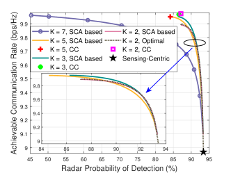
Figure 2: S$\&$C performance tradeoff.

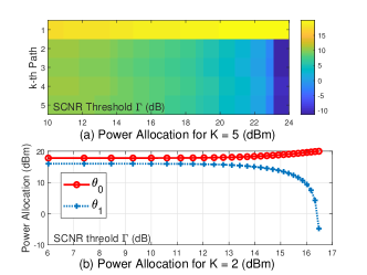
Figure 3: PA with $K=5$ and $K=2$.

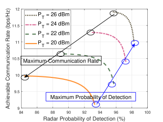
Figure 4: S$\&$C performance versus $P_{T}$.

IV Simulation Results

In this section, we evaluate the proposed algorithm by MonteCarlo based simulation results. Without loss of generality, the reflecting coefficients $\beta_{k}$, and the complex channel gain $\alpha_{k}$ are assumed to obey the standard Complex Gaussian distribution $\mathcal{CN}(0,1)$ and the Rician factor is set as $\varrho=1$. Unless otherwise specified, the maximum transmit power is given as $P_{T}=20$ dBm and the noise power is set as $\sigma_{c}^{2}=\sigma_{r}^{2}=0$ dBm. The target is located at $\theta_{0}=0^{\circ}$ (LoS link) and the clutter sources (NLoS links) are located at $\theta_{1}=-20^{\circ},\theta_{2}=-10^{\circ},\theta_{3}=10^{\circ},\theta_{4}=20^{\circ}$, respectively. The SCNR threshold $\Gamma$ spans from $0$ dB to $\Gamma_{T}$ dB, where $\Gamma_{T}=P_{T}\gamma_{0}$ is the maximum SCNR threshold amputated for avoiding an infeasible case.

We commence by evaluating the S$\&$C performance under different DoFs in Fig. 4 through the proposed approaches, using one pair of benchmarks, namely,

• Sensing-centric (SC) design, which reaches the best sensing performance by setting $p_{0}=P_{T}$, i.e., the ISAC-BS allocates all the power to the LoS link;

• Communication-centric (CC) design, which reaches the maximum achievable communication rate by applying the Cauchy-Schwarz inequality to the objective function of (42), i.e., $(\sum_{k=0}^{K-1}\sqrt{p_{k}}x_{k})^{2}\leq P_{T}(\sum_{k=0}^{K-1}x_{k}^{2})$.

First, we observe that the SCA based method approaches the optimal solution for $K=2$, because the SCA technique reduces the feasible region. Then, we also see that regardless of the spatial DoFs, the achievable maximum radar probability of detection is identical for all cases since the ISAC-BS assigns its total power to the LoS link. By contrast, when the spatial DoFs are higher, our approach usually attains a higher communication rate (see $K=2$, $K=3$, $K=5$ and $K=7$ in Fig. 4). But this is not always true, when we also take the sensing performance into consideration, especially when the radar probability of detection has to be above $90\%$. This is because having higher DoFs for communications imposes more clutter sources, which are harmful to radar sensing. Futhermore, all proposed schemes are capable of attaining a flexible CC or SC trade-off by adjusting the PA among different paths. Again, CC design exploits all available spatial DoFs, while SC design only relies on LoS transmission. We can conclude through Fig. 4 that utilizing flexible spatial DoFs tradeoff is important for achieving scalable S$\&$C performance.

In Fig. 4, we characterize our PA scheme for $K=5$ and $K=2$ respectively based Algorithm 1. Observe that upon increasing the SCNR threshold, the transmit power allocated to the NLoS links is reduced. When the SCNR approaches $\Gamma_{T}$, i.e., the maximum feasibility threshold, the transmit power allocated to the LoS link tends to approach $P_{T}$ for satisfying more strict SCNR threshold requirements. Futhermore, since we assume that both the reflecting coefficients and the complex channel gain are iid, the transmit power of different NLoS links is commensurate (see $K=5$ in Fig. 4(a)).

Finally, in Fig. 4, we show the S$\&$C performance tradeoff vs. $P_{T}$, for $K=5$. The maximum achievable communication rate and the probability of successful detection increase with the maximum transmit power budget. Moreover, the S$\&$C performance region is also extended upon increasing the power budget.

V Conclusions

In this paper, we investigated the S$\&$C performance tradeoffs in terms of the ISAC channel’s DoFs, by proposing a novel transmit power allocating accords the transmit signal propagation paths. We first constructed the parameter estimator and target detector under the signal model considered. Then, we formulated a PA problem for maximizing the achievable communication rate subject to a minimal required radar SCNR constraint and power budget. To gain deeper insights into the problem, the closed-form solution was focused for the case of a single NLoS link. Then, we extended it to the more practical scenario of multiple NLoS links. To tackle the resultant non-convex optimization problem, we harnessed the SCA algorithm, where the transmit power vector is optimized in an iterative manner. Finally, simulation results were provided for characterizing the performance tradeoff between S$\&$C, which suggests that both the S$\&$C performance can be simultaneously optimized by exploiting all ISAC spatial DoFs.

References

- [1] Y. Cui, F. Liu, X. Jing, and J. Mu, “Integrating sensing and communications for ubiquitous IoT: Applications, trends, and challenges,” IEEE Network, vol. 35, no. 5, pp. 158–167, 2021.
- [2] F. Liu, Y. Cui, C. Masouros, J. Xu, T. X. Han, Y. C. Eldar, and S. Buzzi, “Integrated sensing and communications: Towards dual-functional wireless networks for 6G and beyond,” IEEE J. Sel. Areas Commun., pp. 1–1, early access, 2022, doi: 10.1109/JSAC.2022.3156632.
- [3] F. Liu, W. Yuan, C. Masouros, and J. Yuan, “Radar-assisted predictive beamforming for vehicular links: Communication served by sensing,” IEEE Trans. Wireless Commun., vol. 19, no. 11, pp. 7704–7719, 2020.
- [4] N. Su, F. Liu, Z. Wei, Y.-F. Liu, and C. Masouros, “Secure dual-functional radar-communication transmission: Exploiting interference for resilience against target eavesdropping,” IEEE Trans. Wireless Commun., 2022.
- [5] G. Li, S. Wang, J. Li, R. Wang, F. Liu, M. Zhang, X. Peng, and T. X. Han, “Rethinking the tradeoff in integrated sensing and communication: Recognition accuracy versus communication rate,” arXiv preprint arXiv:2107.09621, 2021.
- [6] J. Yang, G. Cui, X. Yu, and L. Kong, “Dual-use signal design for radar and communication via ambiguity function sidelobe control,” IEEE Trans. Veh. Technol., vol. 69, no. 9, pp. 9781–9794, 2020.
- [7] R. Zhang, B. Shim, W. Yuan, M. Di Renzo, X. Dang, and W. Wu, “Integrated sensing and communication waveform design with sparse vector coding: Low sidelobes and ultra reliability,” IEEE Trans. Veh. Technol., 2022.
- [8] X. Wang, Z. Fei, Z. Zheng, and J. Guo, “Joint waveform design and passive beamforming for ris-assisted dual-functional radar-communication system,” IEEE Trans. Veh. Technol., vol. 70, no. 5, pp. 5131–5136, 2021.
- [9] E. Fishler, A. Haimovich, R. S. Blum, L. J. Cimini, D. Chizhik, and R. A. Valenzuela, “Spatial diversity in radars—models and detection performance,” IEEE Trans. Signal Process., vol. 54, no. 3, pp. 823–838, 2006.
- [10] L. Xu, J. Li, and P. Stoica, “Target detection and parameter estimation for MIMO radar systems,” IEEE Trans. Aerosp. Electron. Syst., vol. 44, no. 3, pp. 927–939, 2008.
- [11] G. Cui, H. Li, and M. Rangaswamy, “MIMO radar waveform design with constant modulus and similarity constraints,” IEEE Trans. Signal Process., vol. 62, no. 2, pp. 343–353, 2013.
- [12] X. Liu, T. Huang, N. Shlezinger, Y. Liu, J. Zhou, and Y. C. Eldar, “Joint transmit beamforming for multiuser MIMO communications and MIMO radar,” IEEE Trans. Signal Process., vol. 68, pp. 3929–3944, 2020.
- [13] S. M. Kay, Fundamentals of statistical signal processing: estimation theory. Prentice-Hall, Inc., 1993.
- [14] S. Boyd, S. P. Boyd, and L. Vandenberghe, Convex optimization. Cambridge university press, 2004.