Efficient Representation of Large-Alphabet Probability Distributions

Abstract

A number of engineering and scientific problems require representing and manipulating probability distributions over large alphabets, which we may think of as long vectors of reals summing to $1$. In some cases it is required to represent such a vector with only $b$ bits per entry. A natural choice is to partition the interval $[0,1]$ into $2^{b}$ uniform bins and quantize entries to each bin independently. We show that a minor modification of this procedure – applying an entrywise non-linear function (compander) $f(x)$ prior to quantization – yields an extremely effective quantization method. For example, for $b=8(16)$ and $10^{5}$-sized alphabets, the quality of representation improves from a loss (under KL divergence) of $0.5(0.1)$ bits/entry to $10^{-4}(10^{-9})$ bits/entry. Compared to floating point representations, our compander method improves the loss from $10^{-1}(10^{-6})$ to $10^{-4}(10^{-9})$ bits/entry. These numbers hold for both real-world data (word frequencies in books and DNA $k$-mer counts) and for synthetic randomly generated distributions. Theoretically, we analyze a minimax optimality criterion and show that the closed-form compander $f(x)\leavevmode\nobreak\ \propto\leavevmode\nobreak\ \mathrm{ArcSinh}(\sqrt{c_{K}(K\log K)x})$ is (asymptotically as $b\to\infty$) optimal for quantizing probability distributions over a $K$-letter alphabet. Non-asymptotically, such a compander (substituting $1/2$ for $c_{K}$ for simplicity) has KL-quantization loss bounded by $\leq 8\cdot 2^{-2b}\log^{2}K$. Interestingly, a similar minimax criterion for the quadratic loss on the hypercube shows optimality of the standard uniform quantizer. This suggests that the $\mathrm{ArcSinh}$ quantizer is as fundamental for KL-distortion as the uniform quantizer for quadratic distortion.

I Compander Basics and Definitions

Consider the problem of quantizing the probability simplex $\triangle_{K-1}=\{{\boldsymbol{x}}\in{\mathbb{R}}^{K}:{\boldsymbol{x}}\geq{\boldsymbol{0}},\sum_{i}x_{i}=1\}$ of alphabet size $K$, i.e. of finding a finite subset $\mathcal{Z}\subseteq\triangle_{K-1}$ to represent the entire simplex. Each ${\boldsymbol{x}}\in\triangle_{K-1}$ is associated with some $\boldsymbol{z}=\boldsymbol{z}({\boldsymbol{x}})\in\mathcal{Z}$, and the objective is to find a set $\mathcal{Z}$ and an assignment such that the difference between the values ${\boldsymbol{x}}\in\triangle_{K-1}$ and their representations $\boldsymbol{z}\in\mathcal{Z}$ are minimized; while this can be made arbitrarily small by making $\mathcal{Z}$ arbitrarily large, the goal is to do this efficiently for any given fixed size $|\mathcal{Z}|=M$. Since ${\boldsymbol{x}},\boldsymbol{z}\in\triangle_{K-1}$, they both represent probability distributions over a size-$K$ alphabet. Hence, a natural way to measure the quality of the quantization is to use the KL (Kullback-Leibler) divergence $D_{\operatorname{{\scriptscriptstyle KL}}}({\boldsymbol{x}}\|\boldsymbol{z})$, which corresponds to the excess code length for lossless compression and is commonly used as a way to compare probability distributions. (Note that we want to minimize the KL divergence.)

While one can consider how to best represent the vector ${\boldsymbol{x}}$ as a whole, in this paper we consider only scalar quantization methods in which each element $x_{j}$ of ${\boldsymbol{x}}$ is handled separately, since we showed in [1] that for Dirichlet priors on the simplex, methods using scalar quantization perform nearly as well as optimal vector quantization. Scalar quantization is also typically simpler and faster to use, and can be parallelized easily. Our scalar quantizer is based on companders (portmanteau of ‘compressor’ and ‘expander’), a simple, powerful and flexible technique first explored by Bennett in 1948 [2] in which the value $x_{j}$ is passed through a nonlinear function $f$ before being uniformly quantized. We discuss the background in greater depth in Section III.

In what follows, $\log$ is always base-$e$ unless otherwise specified. We denote $[N]:=\{1,\dots,N\}$.

I-1 Encoding

Companders require two things: a monotonically increasing function $f:[0,1]\to[0,1]$ (we denote the set of such functions as ${\mathcal{F}}$) and an integer $N$ representing the number of quantization levels, or granularity. To simplify the problem and algorithm, we use the same $f$ for each element of the vector ${\boldsymbol{x}}=(x_{1},\dots,x_{K})\in\triangle_{K-1}$ (see Remark 1). To quantize $x\in[0,1]$, the compander computes $f(x)$ and applies a uniform quantizer with $N$ levels, i.e. encoding $x$ to $n_{N}(x)\in[N]$ if $f(x)\in(\frac{n-1}{N},\frac{n}{N}]$; this is equivalent to $n_{N}(x)=\lceil f(x)N\rceil$.

This encoding partitions $[0,1]$ into bins $I^{(n)}$:

$$x\in I^{(n)}=f^{-1}\Big{(}\Big{(}\frac{n-1}{N},\frac{n}{N}\Big{]}\Big{)}\iff n_{N}(x)=n$$ (1)

where $f^{-1}$ denotes the preimage under $f$.

As an example, consider the function $f(x)=x^{s}$. Varying $s$ gives a natural class of functions from $[0,1]$ to $[0,1]$, which we call the class of power companders. If we select $s=1/2$ and $N=4$, then the $4$ bins created by this encoding are

$$I^{(1)} =(0,1/16],I^{(2)}=(1/16,1/4],$$ (2)

$$I^{(3)} =(1/4,9/16],I^{(4)}=(9/16,1]\,.$$ (3)

I-2 Decoding

To decode $n\in[N]$, we pick some $y_{(n)}\in I^{(n)}$ to represent all $x\in I^{(n)}$; for a given $x$ (at granularity $N$), its representation is denoted $y(x)=y_{(n_{N}(x))}$. This is generally either the midpoint of the bin or, if $x$ is drawn randomly from a known prior $p$, the centroid (the mean within bin $I^{(n)}$). The midpoint and centroid of $I^{(n)}$ are defined, respectively, as

$$\bar{y}_{(n)} ={1\over 2}\left(f^{-1}\left(\frac{n-1}{N}\right)+f^{-1}\left(\frac{n}{N}\right)\right)$$ (4)

$$\widetilde{y}_{(n)} ={\mathbb{E}}_{X\sim p}[X\,|\,X\in I^{(n)}]\,.$$ (5)

We will discuss this in greater detail in Section I-4.

Handling each element of ${\boldsymbol{x}}$ separately means the decoded values may not sum to $1$, so we normalize the vector after decoding. Thus, if ${\boldsymbol{x}}$ is the input,

$$z_{i}({\boldsymbol{x}})=\frac{y(x_{i})}{\sum_{j=1}^{K}y(x_{j})}$$ (6)

and the vector $\boldsymbol{z}=\boldsymbol{z}({\boldsymbol{x}})=(z_{1}({\boldsymbol{x}}),\dots,z_{K}({\boldsymbol{x}}))\in\triangle_{K-1}$ is the output of the compander. This notation reflects the fact that each entry of the normalized reconstruction depends on all of ${\boldsymbol{x}}$ due to the normalization step. We refer to $\boldsymbol{y}=\boldsymbol{y}({\boldsymbol{x}})=(y(x_{1}),\dots,y(x_{K}))$ as the raw reconstruction of ${\boldsymbol{x}}$, and $\boldsymbol{z}$ as the normalized reconstruction. If the raw reconstruction uses centroid decoding, we likewise denote it using $\widetilde{{\boldsymbol{y}}}=\widetilde{{\boldsymbol{y}}}({\boldsymbol{x}})=(\widetilde{y}(x_{1}),\dots,\widetilde{y}(x_{K}))$. For brevity we may sometimes drop the ${\boldsymbol{x}}$ input in the notation, e.g. ${\boldsymbol{z}}:={\boldsymbol{z}}({\boldsymbol{x}})$; if ${\boldsymbol{X}}$ is random we will sometimes denote its quantization as ${\boldsymbol{Z}}:={\boldsymbol{z}}({\boldsymbol{X}})$.

Thus, any ${\boldsymbol{x}}\in\triangle_{K-1}$ requires $K\lceil\log_{2}N\rceil$ bits to store; to encode and decode, only $f$ and $N$ need to be stored (as well as the prior if using centroid decoding). Another major advantage is that a single $f$ can work well over many or all choices of $N$, making the design more flexible.

I-3 KL divergence loss

The loss incurred by representing ${\boldsymbol{x}}$ as $\boldsymbol{z}:=\boldsymbol{z}({\boldsymbol{x}})$ is the KL divergence

$$D_{\operatorname{{\scriptscriptstyle KL}}}({\boldsymbol{x}}\|\boldsymbol{z})=\sum_{i=1}^{K}x_{i}\log\frac{x_{i}}{z_{i}}\,.$$ (7)

Although this loss function has some unusual properties (for instance $D_{\operatorname{{\scriptscriptstyle KL}}}({\boldsymbol{x}}\|\boldsymbol{z})\neq D_{\operatorname{{\scriptscriptstyle KL}}}(\boldsymbol{z}\|{\boldsymbol{x}})$ and it does not obey the triangle inequality) it measures the amount of ‘mis-representation’ created by representing the probability vector ${\boldsymbol{x}}$ by another probability vector $\boldsymbol{z}$, and is hence is a natural quantity to minimize. In particular, it represents the excess code length created by trying to encode the output of ${\boldsymbol{x}}$ using a code built for $\boldsymbol{z}$, as well as having connections to hypothesis testing (a natural setting in which the ‘difference’ between probability distributions is studied).

I-4 Distributions from a prior

Much of our work concerns the case where ${\boldsymbol{x}}\in\triangle_{K-1}$ is drawn from some prior $P_{\boldsymbol{x}}$ (to be commonly denoted as simply $P$). Using a single $f$ for each entry means we can WLOG assume that $P$ is symmetric over the alphabet, i.e. for any permutation $\sigma$, if ${\boldsymbol{X}}\sim P$ then $\sigma({\boldsymbol{X}})\sim P$ as well. This is because for any prior $P$ over $\triangle_{K-1}$, there is a symmetric prior $P^{\prime}$ such that

$${\mathbb{E}}_{{\boldsymbol{X}}\sim P}[D_{\operatorname{{\scriptscriptstyle KL}}}({\boldsymbol{X}}\|\boldsymbol{z}({\boldsymbol{X}}))]={\mathbb{E}}_{{\boldsymbol{X}}^{\prime}\sim P^{\prime}}[D_{\operatorname{{\scriptscriptstyle KL}}}({\boldsymbol{X}}^{\prime}\|\boldsymbol{z}({\boldsymbol{X}}^{\prime}))]$$ (8)

for all $f$, where $\boldsymbol{z}({\boldsymbol{X}})$ is the result of quantizing (to any number of levels) with $f$ as the compander. To get ${\boldsymbol{X}}^{\prime}\sim P^{\prime}$, generate ${\boldsymbol{X}}\sim P$ and a uniformly random permutation $\sigma$, and let ${\boldsymbol{X}}^{\prime}=\sigma({\boldsymbol{X}})$.

We denote the set of symmetric priors as ${\mathcal{P}}^{\triangle}_{K}$. Note that a key property of symmetric priors is that their marginal distributions are the same across all entries, and hence we can speak of $P\in{\mathcal{P}}^{\triangle}_{K}$ having a single marginal $p$.

Remark 1.

In principle, given a nonsymmetric prior $P_{\boldsymbol{x}}$ over $\triangle_{K-1}$ with marginals $p_{1},\dots,p_{K}$, we could quantize each letter’s value with a different compander $f_{1},\dots,f_{K}$, giving more accuracy than using a single $f$ (at the cost of higher complexity). However, the symmetrization of $P_{\boldsymbol{x}}$ over the letters (by permuting the indices randomly after generating ${\boldsymbol{X}}\sim P_{\boldsymbol{x}}$) yields a prior in ${\mathcal{P}}^{\triangle}_{K}$ on which any single $f$ will have the same (overall) performance and cannot be improved on by using varying $f_{i}$. Thus, considering symmetric $P_{\boldsymbol{x}}$ suffices to derive our minimax compander.

While the random probability vector comes from a prior $P\in{\mathcal{P}}^{\triangle}_{K}$, our analysis will rely on decomposing the loss so we can deal with one letter at a time. Hence, we work with the marginals $p$ of $P$ (which are identical since $P$ is symmetric), which we refer to as single-letter distributions and are probability distributions over $[0,1]$.

We let ${\mathcal{P}}$ denote the class of probability distributions over $[0,1]$ that are absolutely continuous with respect to the Lebesgue measure. We denote elements of ${\mathcal{P}}$ by their probability density functions (PDF), e.g. $p\in{\mathcal{P}}$; the cumulative distribution function (CDF) associated with $p$ is denoted $F_{p}$ and satisfies $F^{\prime}_{p}(x)=p(x)$ and $F_{p}(x)=\int_{0}^{x}p(t)\,dt$ (since $F_{p}$ is monotonic, its derivative exists almost everywhere). Note that while $p\in{\mathcal{P}}$ does not have to be continuous, its CDF $F_{p}$ must be absolutely continuous. Following common terminology [3], we refer to such probability distributions as continuous.

Let ${\mathcal{P}}_{1/K}=\{p\in{\mathcal{P}}:{\mathbb{E}}_{X\sim p}[X]=1/K\}$. Note that $P\in{\mathcal{P}}^{\triangle}_{K}$ implies its marginals $p$ are in ${\mathcal{P}}_{1/K}$.

I-5 Expected loss and preliminary results

For $P\in{\mathcal{P}}^{\triangle}_{K}$, $f\in{\mathcal{F}}$ and granularity $N$, we define the expected loss:

$${\mathcal{L}}_{K}(P,f,N)={\mathbb{E}}_{{\boldsymbol{X}}\sim P}[D_{\operatorname{{\scriptscriptstyle KL}}}({\boldsymbol{X}}\|\boldsymbol{z}({\boldsymbol{X}}))]\,.$$ (9)

This is the value we want to minimize over $f$.

Remark 2.

While ${\boldsymbol{X}}$ and $\boldsymbol{z}({\boldsymbol{X}})$ are random, they are also probability vectors. The KL divergence $D_{\operatorname{{\scriptscriptstyle KL}}}({\boldsymbol{X}}\|\boldsymbol{z}({\boldsymbol{X}}))$ is the divergence between ${\boldsymbol{X}}$ and $\boldsymbol{z}({\boldsymbol{X}})$ themselves, not the prior distributions over $\triangle_{K-1}$ they are drawn from.

Note that ${\mathcal{L}}_{K}(P,f,N)$ can almost be decomposed into a sum of $K$ separate expected values, except the normalization step (6) depends on the random vector ${\boldsymbol{X}}$ as a whole. Hence, we define the raw loss:

$$\widetilde{{\mathcal{L}}}_{K}(P,f,N)={\mathbb{E}}_{{\boldsymbol{X}}\sim P}\Big{[}\sum_{i=1}^{K}X_{i}\log(X_{i}/\widetilde{y}(X_{i}))\Big{]}\,.$$ (10)

We also define for $p\in{\mathcal{P}}$, the single-letter loss as

$$\widetilde{L}(p,f,N)={\mathbb{E}}_{X\sim p}\big{[}X\log(X/\widetilde{y}(X))\big{]}\,.$$ (11)

The raw loss is useful because it bounds the (normalized) expected loss and is decomposable into single-letter losses. Note that both raw and single-letter loss are defined with centroid decoding.

Proposition 1.

For $P\in{\mathcal{P}}^{\triangle}_{K}$ with marginals $p$,

$${\mathcal{L}}_{K}(P,f,N)\leq\widetilde{{\mathcal{L}}}_{K}(P,f,N)=K\,\widetilde{L}(p,f,N)\,.$$ (12)

Proof.

Separating out the normalization term gives

$${\mathcal{L}} (P,f,N)={\mathbb{E}}_{{\boldsymbol{X}}\sim P}[D_{\operatorname{{\scriptscriptstyle KL}}}({\boldsymbol{X}}||\boldsymbol{z}({\boldsymbol{X}}))]$$

$$=\widetilde{{\mathcal{L}}}_{K}(P,f,N)+{\mathbb{E}}_{{\boldsymbol{X}}\sim P}\left[\log\left(\sum_{i=1}^{K}\widetilde{y}(X_{i})\right)\right]\,.$$ (13)

Since ${\mathbb{E}}[\widetilde{y}(X_{i})]={\mathbb{E}}[X_{i}]$ for all $i$, $\sum_{i=1}^{K}{\mathbb{E}}[\widetilde{y}(X_{i})]=\sum_{i=1}^{K}{\mathbb{E}}[{X}_{i}]=1$. Because $\log$ is concave, by Jensen’s Inequality

$${\mathbb{E}}_{{\boldsymbol{X}}\sim P}\bigg{[}\log\Big{(}\sum_{i=1}^{K}\widetilde{y}(X_{i})\Big{)}\bigg{]} \leq\log\Big{(}{\mathbb{E}}\Big{[}\sum_{i=1}^{K}\widetilde{y}(X_{i})\Big{]}\Big{)}$$ (14)

$$=\log(1)=0$$ (15)

and we are done. ∎

To derive our results about worst-case priors (for instance, Theorem 1), we will also be interested in $\widetilde{L}(p,f,N)$ even when $p$ is not known to be a marginal of some $P\in{\mathcal{P}}^{\triangle}_{K}$.

Remark 3.

Though one can define raw and single-letter loss without centroid decoding (replacing $\widetilde{y}$ in (10) or (11) with another decoding method $\widehat{y}$), this removes much of their usefulness. This is because the resulting expected loss can be dominated by the difference between ${\mathbb{E}}[X]$ and ${\mathbb{E}}[\widehat{y}(X)]$, potentially even making it negative; specifically, the Taylor expansion of $X\log(X/\widehat{y}(X))$ has $X-\widehat{y}(X)$ in its first term, which can have negative expectation.

While this can make the expected ‘raw loss’ negative under general decoding, it cannot be exploited to make the (normalized) expected loss negative because the normalization step $z_{i}({\boldsymbol{X}})=\widehat{y}(X_{i})/\sum_{j}\widehat{y}(X_{j})$ cancels out the problematic term. Centroid decoding avoids this problem by ensuring ${\mathbb{E}}[X]={\mathbb{E}}[\widetilde{y}(X)]$, removing the issue.

As we will show, when $N$ is large these values are roughly proportional to $N^{-2}$ (for well-chosen $f$) and so we define the asymptotic single-letter loss:

$$\widetilde{L}(p,f)=\lim_{N\to\infty}N^{2}\widetilde{L}(p,f,N)\,.$$ (16)

We similarly define $\widetilde{{\mathcal{L}}}_{K}(P,f)$ and ${\mathcal{L}}_{K}(P,f)$. While the limit in (16) does not necessarily exist for every $p,f$, we will show that one can ensure it exists by choosing an appropriate $f$ (which works against any $p\in{\mathcal{P}}$), and cannot gain much by not doing so.

II Results

We demonstrate, theoretically and experimentally, the efficacy of companding for quantizing probability distributions with KL divergence loss.

II-A Theoretical Results

While we will occasionally give intuition for how the results here are derived, our primary concern in this section is to fully state the results and to build a clear framework for discussing them.

Our main results concern the formulation and evaluation of a minimax compander $f^{*}_{K}$ for alphabet size $K$, which satisfies

$$f^{*}_{K}=\underset{f\,\in\,{\mathcal{F}}}{{\mathrm{arg}\min}}\underset{p\,\in\,{\mathcal{P}}_{1/K}}{\sup}\widetilde{L}(p,f)\,.$$ (17)

We require $p\in{\mathcal{P}}_{1/K}$ because if $P\in{\mathcal{P}}^{\triangle}_{K}$ and is symmetric, its marginals are in ${\mathcal{P}}_{1/K}$.

The natural counterpart of the minimax compander $f^{*}_{K}$ is the maximin density $p^{*}_{K}\in{\mathcal{P}}_{1/K}$, satisfying

$$p^{*}_{K}=\underset{p\,\in\,{\mathcal{P}}_{1/K}}{{\mathrm{arg}\max}}\underset{f\,\in\,{\mathcal{F}}}{\inf}\widetilde{L}(p,f)\,.$$ (18)

We call (17) and (18), respectively, the minimax condition and the maximin condition.

In the same way that the minimax compander gives the best performance guarantee against an unknown single-letter prior $p\in{\mathcal{P}}_{1/K}$ (asymptotic as $N\to\infty$), the maximin density is the most difficult prior to quantize effectively as $N\to\infty$. Since they are highly related, we will define them together:

Proposition 2.

For alphabet size $K>4$, there is a unique $c_{K}\in[\frac{1}{4},\frac{3}{4}]$ such that if $a_{K}=(4/(c_{K}K\log K+1))^{1/3}$ and $b_{K}=4/a_{K}^{2}-a_{K}$, then the following density is in ${\mathcal{P}}_{1/K}$:

$$p^{*}_{K}(x)=(a_{K}x^{1/3}+b_{K}x^{4/3})^{-3/2}\,.$$ (19)

Furthermore, $\lim_{K\to\infty}c_{K}=1/2$.

Note that this is both a result and a definition: we show that $a_{K},b_{K},c_{K}$ exist which make the definition of $p^{*}_{K}$ possible. With the constant $c_{K}$, we define the minimax compander:

Definition 1.

Given the constant $c_{K}$ as shown to exist in Proposition 2, the minimax compander is the function $f^{*}_{K}:[0,1]\to[0,1]$ where

$$f^{*}_{K}(x)=\frac{\mathrm{ArcSinh}(\sqrt{c_{K}(K\log K)\,x})}{\mathrm{ArcSinh}(\sqrt{c_{K}K\log K})}\,.$$ (20)

The approximate minimax compander $f^{**}_{K}$ is

$$f^{**}_{K}(x)=\frac{\mathrm{ArcSinh}(\sqrt{(1/2)(K\log K)\,x})}{\mathrm{ArcSinh}(\sqrt{(1/2)K\log K})}\,.$$ (21)

Remark 4.

While $f^{*}_{K}$ and $f^{**}_{K}$ might seem complex, $\mathrm{ArcSinh}(\sqrt{w})=\log(\sqrt{w}+\sqrt{w+1})$ so they are relatively simple functions to work with.

We will show that $f^{*}_{K},p^{*}_{K}$ as defined above satisfy their respective conditions (17) and (18):

Theorem 1.

The minimax compander $f^{*}_{K}$ and maximin single-letter density $p^{*}_{K}$ satisfy

$$\sup_{p\in{\mathcal{P}}_{1/K}}\widetilde{L}(p,f^{*}_{K})=\inf_{f\in{\mathcal{F}}}\sup_{p\in{\mathcal{P}}_{1/K}}\widetilde{L}(p,f)$$ (22)

$$= \sup_{p\in{\mathcal{P}}_{1/K}}\inf_{f\in{\mathcal{F}}}\widetilde{L}(p,f)=\inf_{f\in{\mathcal{F}}}\widetilde{L}(p^{*}_{K},f)$$ (23)

which is equal to $\widetilde{L}(p^{*}_{K},f^{*}_{K})$ and satisfies

$$\widetilde{L}(p^{*}_{K},f^{*}_{K})=\frac{1}{24}(1+o(1))K^{-1}\log^{2}K.$$ (24)

Since any symmetric $P\in{\mathcal{P}}^{\triangle}_{K}$ has marginals $p\in{\mathcal{P}}_{1/K}$, this (with Proposition 1) implies an important corollary for the normalized KL-divergence loss incurred by using the minimax compander:

Corollary 1.

For any prior $P\in{\mathcal{P}}^{\triangle}_{K}$,

$${\mathcal{L}}_{K}(P,f^{*}_{K})\leq\widetilde{{\mathcal{L}}}_{K}(P,f^{*}_{K})=\frac{1}{24}(1+o(1))\log^{2}K\,.$$ (25)

However, the set of symmetric $P\in{\mathcal{P}}^{\triangle}_{K}$ does not correspond exactly with $p\in{\mathcal{P}}_{1/K}$: while any symmetric $P\in{\mathcal{P}}^{\triangle}_{K}$ has marginals $p\in{\mathcal{P}}_{1/K}$, it is not true that any given $p\in{\mathcal{P}}_{1/K}$ has a corresponding symmetric prior $P\in{\mathcal{P}}^{\triangle}_{K}$. Thus, it is natural to ask: can the minimax compander’s performance be improved by somehow taking these ‘shape’ constraints into account? The answer is ‘not by more than a factor of $\approx 2$’:

Proposition 3.

There is a prior $P^{*}\in{\mathcal{P}}^{\triangle}_{K}$ such that for any $P\in{\mathcal{P}}^{\triangle}_{K}$

$$\inf_{f\in{\mathcal{F}}}\widetilde{{\mathcal{L}}}_{K}(P^{*},f)\geq\frac{K-1}{2K}\widetilde{{\mathcal{L}}}_{K}(P,f^{*}_{K})\,.$$ (26)

While the minimax compander satisfies the minimax condition (17), it requires working with the constant $c_{K}$, which, while bounded, is tricky to compute or use exactly. Hence, in practice we advocate using the approximate minimax compander (21), which yields very similar asymptotic performance without needing to know $c_{K}$:

Proposition 4.

Suppose that $K$ is sufficiently large so that $c_{K}\in[\frac{1}{2(1+\varepsilon)},\frac{1+\varepsilon}{2}]$. Then for any $p\in{\mathcal{P}}$,

$$\widetilde{L}(p,f^{**}_{K})\leq(1+\varepsilon)\widetilde{L}(p,f^{*}_{K})\,.$$ (27)

Before we show how we get Theorem 1, we make the following points:

Remark 5.

If we use the uniform quantizer instead of minimax there exists a $P\in{\mathcal{P}}^{\triangle}_{K}$ where

$${\mathbb{E}}_{{\boldsymbol{X}}\sim P}[D_{\operatorname{{\scriptscriptstyle KL}}}({\boldsymbol{X}}\|\boldsymbol{Z})]=\Theta\left(K^{2}N^{-2}\log N\right)\,.$$ (28)

This is done by using marginal density $p$ uniform on $[0,2/K]$. To get a prior $P\in{\mathcal{P}}^{\triangle}_{K}$ with these marginals, if $K$ is even, we can pair up indices so that $x_{2j-1}=2/K-x_{2j}$ for all $j=1,\dots,K/2$ (for odd $K$, set $x_{K}=1/K$) and then symmetrize by permuting the indices. See Appendix F for more details.

The dependence on $N$ is worse than $N^{-2}$ resulting in $\widetilde{L}(p,f)=\infty$. This shows theoretical suboptimality of the uniform quantizer. Note also that the quadratic dependence on $K$ is significantly worse than the $\log^{2}K$ dependence achieved by the minimax compander.

Incidentally, other single-letter priors such as $p(x)=(1-\alpha)x^{-\alpha}$ where $\alpha=\frac{K-2}{K-1}$ can achieve worse dependence on $N$ (specifically, $N^{-(2-\alpha)}$ for this prior). However, the example above achieves a bad dependence on both $N$ and $K$ simultaneously, showing that in all regimes of $K,N$ the uniform quantizer is vulnerable to bad priors.

Remark 6.

Instead of the KL divergence loss on the simplex, we can do a similar analysis to find the minimax compander for $L_{2}^{2}$ loss on the unit hypercube. The solution is given by the identity function $f(x)=x$ corresponding to the standard (non-companded) uniform quantization. (See Section VI.)

To show Theorem 1 we formulate and show a number of intermediate results which are also of significant interest for a theoretical understanding of companding under KL divergence, in particular studying the asymptotic behavior of $\widetilde{L}(p,f,N)$ as $N\to\infty$. We define:

Definition 2.

For $p\in{\mathcal{P}}$ and $f\in{\mathcal{F}}$, let

$$L^{\dagger}(p,f) =\frac{1}{24}\int_{0}^{1}p(x)f^{\prime}(x)^{-2}x^{-1}\,dx$$ (29)

$$={\mathbb{E}}_{X\sim p}\Big{[}\frac{1}{24}f^{\prime}(X)^{-2}X^{-1}\Big{]}\,.$$ (30)

For full rigor, we also need to define a set of ‘well-behaved’ companders:

Definition 3.

Let ${\mathcal{F}}^{\dagger}\subseteq{\mathcal{F}}$ be the set of $f$ such that for each $f$ there exist constants $c>0$ and $\alpha\in(0,1/2]$ for which $f(x)-cx^{\alpha}$ is still monotonically increasing.

Then the following describes the asymptotic single-letter loss of compander $f$ on prior $p$ (with centroid decoding):

Theorem 2.

For any $p\in{\mathcal{P}}$ and $f\in{\mathcal{F}}$,

$$\liminf_{N\to\infty}N^{2}\widetilde{L}(p,f,N)\geq L^{\dagger}(p,f)\,.$$ (31)

Furthermore, if $f\in{\mathcal{F}}^{\dagger}$ then an exact result holds:

$$\widetilde{L}(p,f) =L^{\dagger}(p,f)<\infty\,.$$ (32)

The intuition behind the formula for $L^{\dagger}(p,f)$ is that as $N\to\infty$, the density $p$ becomes roughly uniform within each bin $I^{(n)}$. Additionally, the bin containing a given $x\in[0,1]$ will have width $r_{(n)}\approx N^{-1}f^{\prime}(x)^{-1}$. Then, letting ${\mathrm{unif}}_{I^{(n)}}$ be the uniform distribution over $I^{(n)}$ and $\bar{y}_{(n)}\approx x$ be the midpoint of $I^{(n)}$ (which is also the centroid under the uniform distribution), we apply the approximation

$${\mathbb{E}}_{X\sim{\mathrm{unif}}_{I^{(n)}}}[X\log(X/\bar{y}_{(n)})] \approx\frac{1}{24}r_{(n)}^{2}\bar{y}_{(n)}^{-1}$$ (33)

$$\approx\frac{1}{24}N^{-2}f^{\prime}(x)^{-2}x^{-1}\,.$$ (34)

Averaging over $X\sim p$ and multiplying by $N^{2}$ then gives (30). One wrinkle is that we need to use the Dominated Convergence Theorem to get the exact result (32), but we cannot necessarily apply it for all $f\in{\mathcal{F}}$; instead, we can apply it for all $f\in{\mathcal{F}}^{\dagger}$, and outside of ${\mathcal{F}}^{\dagger}$ we get (31) using Fatou’s Lemma.

While limiting ourselves to $f\in{\mathcal{F}}^{\dagger}$ might seem like a serious restriction, it does not lose anything essential because ${\mathcal{F}}^{\dagger}$ is ‘dense’ within ${\mathcal{F}}$ in the following way:

Proposition 5.

For any $f\in{\mathcal{F}}$ and $\delta\in(0,1]$,

$$f_{\delta}(x)=(1-\delta)f(x)+\delta x^{1/2}$$ (35)

satisfies $f_{\delta}\in{\mathcal{F}}^{\dagger}$ and

$$\lim_{\delta\to 0}\widetilde{L}(p,f_{\delta})=\lim_{\delta\to 0}L^{\dagger}(p,f_{\delta})=L^{\dagger}(p,f)\,.$$ (36)

Remark 7.

It is important to note that strictly speaking the limit represented by $\widetilde{L}(p,f)$ may not always exist if $f\not\in{\mathcal{F}}^{\dagger}$. However: (i) one can always guarantee that it exists by selecting $f\in{\mathcal{F}}^{\dagger}$; (ii) by (31), it is impossible to use $f$ outside ${\mathcal{F}}^{\dagger}$ to get asymptotic performance better than $L^{\dagger}(p,f)$; and (iii) by Proposition 5, given $f$ outside ${\mathcal{F}}^{\dagger}$, one can get a compander in ${\mathcal{F}}^{\dagger}$ with arbitrarily close (or better) performance to $f$ by using $f_{\delta}(x)=(1-\delta)f(x)+\delta x^{1/2}$ for $\delta$ close to $0$. This suggests that considering only $f\in{\mathcal{F}}^{\dagger}$ is sufficient since there is no real way to benefit by using $f\not\in{\mathcal{F}}^{\dagger}$.

Additionally, both $f^{*}_{K}$ and $f^{**}_{K}$ are in ${\mathcal{F}}^{\dagger}$. Thus, in Theorem 1, although the limit might not exist for certain $f\in{\mathcal{F}},p\in{\mathcal{P}}_{1/K}$, the minimax compander still performs better since it has less loss than even the $\liminf$ of the loss of other companders.

Given Theorem 2, it’s natural to ask: for a given $p\in{\mathcal{P}}$, what compander $f$ minimizes $L^{\dagger}(p,f)$? This yields the following by calculus of variations:

Theorem 3.

The best loss against source $p\in{\mathcal{P}}$ is

$$\inf_{f\in{\mathcal{F}}}\widetilde{L}(p,f) =\min_{f\in{\mathcal{F}}}L^{\dagger}(p,f)$$ (37)

$$=\frac{1}{24}\Big{(}\int_{0}^{1}(p(x)x^{-1})^{1/3}dx\Big{)}^{3}$$ (38)

where the optimal compander against $p$ is

$$f_{p}(x)=\underset{f\in{\mathcal{F}}}{{\mathrm{arg}\min}}L^{\dagger}(p,f)=\frac{\int_{0}^{x}(p(t)t^{-1})^{1/3}\,dt}{\int_{0}^{1}(p(t)t^{-1})^{1/3}\,dt}$$ (39)

(satisfying $f^{\prime}_{p}(x)\,\propto\,(p(x)x^{-1})^{1/3}$).

Note that $f_{p}$ may not be in ${\mathcal{F}}^{\dagger}$ (for instance, if $p$ assigns zero probability mass to an interval $I\subseteq[0,1]$, then $f_{p}$ will be constant over $I$). However, this can be corrected by taking a convex combination with $x^{1/2}$ as described in Proposition 5.

The expression (38) represents in a sense how hard $p\in{\mathcal{P}}$ is to quantize with a compander, and the maximin density $p^{*}_{K}$ is the density in ${\mathcal{P}}_{1/K}$ which maximizes it; in turn, the minimax compander $f^{*}_{K}$ is the optimal compander against $p^{*}_{K}$, i.e.

$$f^{*}_{K}=f_{p^{*}_{K}}\,.$$ (40)

So far we considered quantization of a random probability vector with a known prior. We next consider the case where the quantization guarantee is given pointwise, i.e. we cover $\triangle_{K-1}$ with a finite number of KL divergence balls of fixed radius. Note that since the prior is unknown, only the midpoint decoder can be used.

Theorem 4 (Divergence covering).

On alphabet size $K>4$ and $N\geq 8\log(2\sqrt{K\log K}+1)$ intervals, the minimax and approximate minimax companders with midpoint decoding achieve worst-case loss over $\triangle_{K-1}$ of

$$\max_{{\boldsymbol{x}}\in\triangle_{K-1}}D_{\operatorname{{\scriptscriptstyle KL}}}({\boldsymbol{x}}\|\boldsymbol{z})\leq(1+\mathrm{err}(K))N^{-2}\log^{2}K$$ (41)

where $\mathrm{err}(K)$ is an error term satisfying

$$\mathrm{err}(K)\leq 18\frac{\log\log K}{\log K}\leq 7\text{ when }K>4\,.$$ (42)

Note that the non-asymptotic worst-case bound matches (up to a constant factor) the known-prior asymptotic result (24). We remark that condition on $N$ is mild: for example, if $N=256$ (i.e. we are representing the probability vector with $8$ bits per entry), then $N>8\log(2\sqrt{K\log K}+1)$ for all $K\leq 2.6\times 10^{25}$.

Remark 8.

When $b$ is the number of bits used to quantize each value in the probability vector, using the approximate minimax compander yields a worst-case loss on the order of $2^{-2b}\log^{2}K$. In [5] we prove bounds on the optimal loss under arbitrary (vector) quantization of probability vectors and show that this loss is sandwiched between $2^{-2b\frac{K}{K-1}}$ ([5, Proposition 2]) and $2^{-2b\frac{K}{K-1}}\log K$ ([5, Theorem 2]). Thus, the entrywise companders in this work are quite competitive.

We also consider the natural family of power companders $f(x)=x^{s}$, both in terms of average asymptotic raw loss and worst-case non-asymptotic normalized loss. By definition, $f(x)\in{\mathcal{F}}^{\dagger}$ and hence $\widetilde{L}(p,f)$ is well-defined and Theorem 2 applies.

Theorem 5.

The power compander $f(x)=x^{s}$ with exponent $s\in(0,1/2]$ has asymptotic loss

$$\underset{p\in{\mathcal{P}}_{1/K}}{\sup}\widetilde{L}(p,f)=\frac{1}{24}s^{-2}K^{2s-1}\,.$$ (43)

For $K>7$, (43) is minimized by setting $s=\frac{1}{\log K}$ (when $K\leq 7$, $\frac{1}{\log K}>1/2$) and $f(x)=x^{s}$ achieves

$$\underset{p\in{\mathcal{P}}_{1/K}}{\sup}\widetilde{L}(p,f) =\frac{e^{2}}{24}\frac{1}{K}\log^{2}K$$ (44)

$$\text{and }\leavevmode\nobreak\ \leavevmode\nobreak\ \underset{P\in{\mathcal{P}}^{\triangle}_{K}}{\sup}\widetilde{{\mathcal{L}}}(P,f) =\frac{e^{2}}{24}\log^{2}K\,.$$ (45)

Additionally, when $s=\frac{1}{\log K}$, it achieves the following worst-case bound with midpoint decoding for $K>7$ and $N>\frac{e}{2}\log K$:

$$\max_{{\boldsymbol{x}}\in\triangle_{K-1}}D_{\operatorname{{\scriptscriptstyle KL}}}({\boldsymbol{x}}\|\boldsymbol{z}) \leq(1+\mathrm{err}(K,N))\frac{e^{2}}{2}N^{-2}\log^{2}K$$ (46)

$$\text{where }\mathrm{err} (K,N)=\frac{e}{2}\frac{\log K}{N-\frac{e}{2}\log K}\,.$$ (47)

Note in particular that when $N\geq e\log K$, we have $\mathrm{err}(K,N)\leq 1$, giving a bound of $\max_{{\boldsymbol{x}}\in\triangle_{K-1}}D_{\operatorname{{\scriptscriptstyle KL}}}({\boldsymbol{x}}\|\boldsymbol{z})\leq e^{2}N^{-2}\log^{2}K$.

We can think of $s=\frac{1}{\log K}$ as a ‘minimax’ among the class of power companders. This result shows $f(x)=x^{\frac{1}{\log K}}$ has performance within a constant factor of the minimax compander, and hence might be a good alternative.

II-B Experimental Results

We compare the performance of five quantizers, with granularities $N=2^{8}$ and $N=2^{16}$, on three types of datasets of various alphabet sizes:

• Random synthetic distributions drawn from the uniform prior over the simplex: We draw and take the average over 1000 random samples for our results.

• Frequency of words in books: These frequencies are computed from text available on the Natural Language Toolkit (NLTK) libraries for Python. For each text, we get tokens (single words or punctuation) from each text and simply count the occurrence of each token

• Frequency of $k$-mers in DNA: For a given sequence of DNA, the set of $k$-mers are the set of length $k$ substrings which appear in the sequence. We use the human genome as the source for our DNA sequences. Parts of the sequence marked as repeats are removed.

Our quantizers are:

• Approximate Minimax Compander: As given by equation (21). Using the approximate minimax compander is much simpler than the minimax compander since the constant $c_{K}$ does not need to be computed.

• Truncation: Uniform quantization (equivalent to $f(x)=x$), which truncates the least significant bits. This is the natural way of quantizing values in $[0,1]$.

• Float and bfloat16: For 8-bit encodings ($N=2^{8}$), we use a floating point implementation which allocates 4 bits to the exponent and 4 bits to the mantissa. For 16-bit encodings ($N=2^{16}$), we use bfloat16, a standard which is commonly used in machine learning [6].

• Exponential Density Interval (EDI): This is the quantization method we used in an achievability proof in [1]. It is designed for the uniform prior over the simplex.

• Power Compander: Recall that the compander is $f(x)=x^{s}$. We optimize $s$ and find that $s=\frac{1}{\log_{e}K}$ asymptotically minimizes KL divergence, and also gives close to the best performance among power companders empirically. To see the effects of different powers $s$ on the performance of the power compander, see Figure 1.

Because a well-defined prior does not always exist for these datasets (and for simplicity) we use midpoint decoding for all the companders. When a probability value of exactly $0$ appears, we do not use companding and instead quantize the value to $0$, i.e. the value $0$ has its own bin.

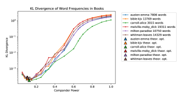
Figure 1: Power compander $f(x)=x^{s}$ performance with different powers $s$ used to quantize frequency of words in books. The number $K$ of distinct words in each book is shown in the legend. The theoretical optimal power $s=\frac{1}{\log K}$ is plotted.

Our main experimental results are given in Figure 2, showing the KL divergence between the empirical distribution ${\boldsymbol{x}}$ and its quantized version $\boldsymbol{z}$ versus alphabet size $K$. The approximate minimax compander performs well against all sources.

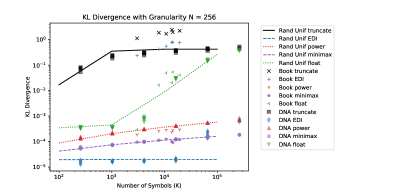
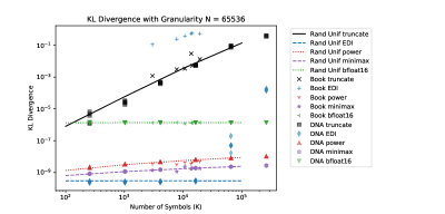
Figure 2: Plot comparing the performance of the truncation compander, the EDI compander, floating points, the power compander, and the approximate minimax compander (21) on probability distributions of various sizes.

For truncation, the KL divergence increases with $K$ and is generally fairly large. The EDI quantizer works well for the synthetic uniform prior (as it should), but for real-world datasets like word frequency in books, it performs badly (sometimes even worse than truncation). The loss of the power compander is similar to the minimax compander (only worse by a constant factor), as predicted by Theorem 5.

The experiments show that the approximate minimax compander achieves low loss on the entire ensemble of data (even for relatively small granularity, such as $N=256$) and outperforms both truncation and floating-point implementations on the same number of bits. Additionally, its closed-form expression (and entrywise application) makes it simple to implement and computationally inexpensive, so it can be easily added to existing systems to lower storage requirements at little or no cost to fidelity.

II-C Paper Organization

We provide background and discuss previous work on companders in Section III. We prove Theorem 2 in Section IV (though proofs of some lemmas and propositions leading up to it are given in Appendix A). Proposition 5 is proved in Appendix B. In Section V, we optimize over (30) to get the maximin single-letter distribution (showing part of Proposition 2 with other parts left to Appendix D-A) and the minimax compander, thus showing Theorems 3 and 1, Corollary 1 and Proposition 3 (leaving Proposition 4 for Appendix D-B). We prove Theorem 4 and the worst-case part of Theorem 5 in Appendix E. Other parts of Theorem 5 are discussed in Appendix C-B. In Section VI we discuss companders for losses other than KL divergence. Finally, in Section VII we discuss a connection of our problem to the problem of information distillation with proofs given in Appendix G.

III Background

Companders (also spelled “compandors”) were introduced by Bennett in 1948 [2] as a way to quantize speech signals, where it is advantageous to give finer quantization levels to weaker signals and coarser levels to larger signals. Bennett gives a first order approximation that the mean-square error in this system is given by

$$\frac{1}{12N^{2}}\int_{a}^{b}\frac{p(x)}{(f^{\prime}(x))^{2}}dx$$ (48)

where $N$ is the number quantization levels, $a$ and $b$ are the minimum and maximum values of the input signal, $p$ is the probability density of the input signal, and $f^{\prime}$ is the slope of the compressor function placed before the uniform quantization. This formula is similar to our (30) except that we have an extra $x^{-1}$ since we are working with KL divergence. Others have expanded on this line of work. In [7], the authors studied the same problem and determined the optimal compressor under mean-square error, a result which parallels our result (38). However, results like those in [2, 7] are stated either as first order approximations or make simplifying assumptions. For example, in [7], the authors state that they assume the values $\widehat{y}_{(n)}$ are close together enough that probability density within any given bin can be treated as a constant. In contrast, we rigorously show that this fundamental logic holds under very general conditions ($f\in{\mathcal{F}}^{\dagger}$).

Generalizations of Bennett’s formula are also studied when instead of mean-square error, the loss is the expected $r$th moment loss ${\mathbb{E}}\|\cdot\|^{r}$. This is computed for vectors of length $K$ in [8] and [9].

The typical examples of companders used in engineering and signals processing are the $\mu$-law and $A$-law companders [10]. For the $\mu$-law compander, [7] and [11] argue that for mean-squared error, for a large enough constant $\mu$ the distortion becomes independent of the signal.

Quantizing probability distributions is a well-studied topic, though typically the loss function is a norm and not KL divergence [12]. Quantizing for KL divergence is considered in our earlier work [1], focusing on average KL loss for Dirichlet priors.

A similar problem to quantizing under KL divergence is information $k$-means. This is the problem of clustering $n$ points $a_{i}$ to $k$ centers $\hat{a}_{j}$ to minimize the KL divergences between the points and their associated centers. Theoretical aspects of this are explored in [13] and [14]. Information $k$-means has been implemented for several different applications [15, 16, 17]. There are also other works that study clustering with a slightly different but related metric [18, 19, 20]; however, the focus of these works is to analyze data rather than reduce storage.

Remark 9.

A variant of the classic problem of prediction with log-loss is an equivalent formulation to quantizing the simplex with KL loss: let ${\boldsymbol{x}}\in\triangle_{K-1}$ and $A\sim{\boldsymbol{x}}$ (in the alphabet $[K]$); we want to predict $A$ by positing a distribution $\boldsymbol{z}\in\triangle_{K-1}$, and our loss is $-\log z_{A}$. In the standard version, the problem is to pick the best $\boldsymbol{z}$ given limited information about ${\boldsymbol{x}}$; however, if we know ${\boldsymbol{x}}$ but are required to express $\boldsymbol{z}$ using only $\log_{2}M$ bits, it is equivalent to quantizing the simplex with KL divergence loss.

IV Asymptotic Single-Letter Loss

In this section we give the proof of Theorem 2 (though the proofs of some lemmas must be sketched). We use the following notation:

Given an interval $I$ we define $\bar{y}_{I}$ to be its midpoint and $r_{I}$ to be its width, so that by definition

$$I=[\bar{y}_{I}-r_{I}/2,\bar{y}_{I}+r_{I}/2]\,.$$ (49)

Note that if $I\subseteq[0,1]$ then $r_{I}\leq 2\bar{y}_{I}$.

Given probability distribution $p$ and interval $I$, we denote the following: $p|_{I}$ is $p$ restricted to $I$; $\pi_{p,I}:={\mathbb{P}}_{X\sim p}[X\in I]$ is the probability mass of $I$; and the centroid of $I$ under $p$ is

$$\widetilde{y}_{p,I}:={\mathbb{E}}_{X\sim p|_{I}}[X]={\mathbb{E}}_{X\sim p}[X\,|\,X\in I]\,.$$ (50)

If they are undefined because ${\mathbb{P}}_{X\sim p}[X\in I]=0$ then by convention $p|_{I}$ is uniform on $I$ and $\widetilde{y}_{p,I}=\bar{y}_{I}$.

When $I=I^{(n)}$ is a bin of the compander, we can replace it with $(n)$ in the notation, i.e. $\bar{y}_{(n)}=\bar{y}_{I^{(n)}}$ (so the midpoint of the bin containing $x$ at granularity $N$ is denoted $\bar{y}_{(n_{N}(x))}$ and the width of the bin is $r_{(n_{N}(x))}$). When $I$ and/or $p$ are fixed, we sometimes drop them from the notation, i.e. $\widetilde{y}_{I}$ or even just $\widetilde{y}$ to denote the centroid of $I$ under $p$.

IV-A The Local Loss Function

One key to the proof is the following perspective: instead of considering $X\sim p$ directly, we (equivalently) first select bin $I^{(n)}$ with probability $\pi_{p,(n)}$, and then select $X\sim p|_{(n)}$. The expected loss can then be considered within bin $I^{(n)}$. This makes it useful to define:

Definition 4.

Given probability measure $p$ and interval $I$, the single-interval loss of $I$ under $p$ is

$$\ell_{p,I}={\mathbb{E}}_{X\sim p|_{I}}[X\log(X/\widetilde{y}_{p,I})]\,.$$ (51)

As before, if $p$ and/or $I$ is fixed and clear, we can drop it from the notation (and if $I=I^{(n)}$ is a bin, we can denote the local loss as $\ell_{p,(n)}$). This can be interpreted as follows: if we quantize all $x\in I$ to the centroid $\widetilde{y}_{I}$, then $\ell_{p,I}$ is the expected loss of $X\sim p$ conditioned on $X\in I$. Thus the values of $\ell_{p,(n)}$ can be used as an alternate means of computing the single-letter loss:

$$\widetilde{L}(p,f,N) ={\mathbb{E}}_{X\sim p}[X\log(X/\widetilde{y}(X))]$$ (52)

$$=\sum_{n=1}^{N}\pi_{p,(n)}{\mathbb{E}}_{X\sim p|_{(n)}}[X\log(X/\widetilde{y}_{p,(n)})]$$ (53)

$$=\sum_{n=1}^{N}\pi_{p,(n)}\ell_{p,(n)}=\int_{[0,1]}\ell_{p,(n_{N}(x))}\,dp\,.$$ (54)

Thus the normalized single-letter loss (whose limit is the asymptotic single-letter loss (16)) is

$$N^{2}\,\widetilde{L}(p,f,N)=\int_{[0,1]}N^{2}\,\ell_{p,(n_{N}(x))}\,dp\,.$$ (55)

For single-letter density $p$ and compander $f$, we define the local loss function at granularity $N$:

$$g_{N}(x)=N^{2}\,\ell_{p,(n_{N}(x))}\,.$$ (56)

We also define the asymptotic local loss function:

$$g(x)=\frac{1}{24}f^{\prime}(x)^{-2}x^{-1}\,.$$ (57)

Theorem 2 is therefore equivalent to:

$$\liminf_{N\to\infty}\int g_{N}\,dp \geq\int g\,dp\leavevmode\nobreak\ \forall\leavevmode\nobreak\ p\in{\mathcal{P}},f\in{\mathcal{F}}$$ (58)

$$\text{and}\,\lim_{N\to\infty}\int g_{N}\,dp =\int g\,dp\leavevmode\nobreak\ \forall\leavevmode\nobreak\ p\in{\mathcal{P}},f\in{\mathcal{F}}^{\dagger}.$$ (59)

To prove (58) and (59), we show:

Proposition 6.

For all $p\in{\mathcal{P}}$, $f\in{\mathcal{F}}$, if $X\sim p$ then

$$\lim_{N\to\infty}g_{N}(X)=g(X)\leavevmode\nobreak\ \leavevmode\nobreak\ \leavevmode\nobreak\ \text{almost surely.}$$ (60)

Proposition 7.

Let $f\in{\mathcal{F}}^{\dagger}$ be a compander and $c>0$ and $\alpha\in(0,1]$ such that $f(x)-cx^{\alpha}$ is monotonically increasing. Letting $g_{N}$ be the local loss functions as in (56) and

$$h(x)=(2^{2/\alpha}+\alpha^{2}2^{1/\alpha-2})(c\alpha)^{-2}x^{1-2\alpha}+c^{-1/\alpha}2^{1/\alpha-2}$$ (61)

then $g_{N}(x)\leq h(x)$ for all $x,N$. Additionally, if $\alpha\leq 1/2$ then $\int_{[0,1]}h\,dp<\infty$.

The lower bound (58) then follows immediately from Proposition 6 and Fatou’s Lemma; and when $f\in{\mathcal{F}}^{\dagger}$, by Proposition 7 there is some $h$ which is integrable over $p$ and dominates all $g_{N}$, thus showing (59) by the Dominated Convergence Theorem.

To prove Proposition 6, we use the following:

• For any $x$ at which $f$ is differentiable, when $N$ is large, the width of the interval $x$ falls in is

  $$r_{(n_{N}(x))}\approx N^{-1}f^{\prime}(x)^{-1}\,.$$ (62)

• For any $x$ at which $F_{p}$ is differentiable, $p|_{I}$ will be approximately uniform over any sufficiently small $I$ containing $x$.

• For a sufficently small interval $I$ containing $x$ and such that $p|_{I}$ is approximately uniform,

  $$\ell_{p,I}\approx\frac{1}{24}r_{I}^{2}x^{-1}\,.$$ (63)

Putting these together, we get that if $F_{p}$ and $f$ are both differentiable at $x$ then when $N$ is large,

$$g_{N}(x) =N^{2}\,\ell_{p,(n_{N}(x))}$$ (64)

$$\approx N^{2}\frac{1}{24}r_{(n_{N}(x))}^{2}x^{-1}\approx\frac{1}{24}f^{\prime}(x)^{-2}x^{-1}=g(x)$$ (65)

as we wanted. We formally state each of these steps in Section A-B and combine them to prove Proposition 6 in Section A-C.

The proof of Proposition 7 is given in Section A-D, along with its own set of definitions and lemmas needed to show it.

V Minimax Compander

Theorem 2 showed that for $f\in{\mathcal{F}}^{\dagger}$, the asymptotic single-letter loss is equivalent to

$$\widetilde{L}(p,f)=\frac{1}{24}\int_{0}^{1}p(x)f^{\prime}(x)^{-2}x^{-1}dx\,.$$ (66)

Using this, we can analyze what is the ‘best’ compander $f$ we can choose and what is the ‘worst’ single-letter density $p$ in order to show Theorems 3 and 1 and their related results.

V-A Optimizing the Compander

We show Theorem 3, which follows from Theorem 2 by finding $f\in{\mathcal{F}}$ which minimizes $L^{\dagger}(p,f)$. This is achieved by optimizing over $f^{\prime}$; we will also use some concepts from Proposition 5 to connect it back to $\inf_{f\in{\mathcal{F}}}\widetilde{L}(p,f)$ when the resulting $f$ is not in ${\mathcal{F}}^{\dagger}$. Since $f:[0,1]\to[0,1]$ is monotonic, we use constraints $f^{\prime}(x)\geq 0$ and $\int_{0}^{1}f^{\prime}(x)\,dx=1$. We solve the following:

minimize $$L^{\dagger}(p,f)=\frac{1}{24}\int_{0}^{1}p(x)f^{\prime}(x)^{-2}x^{-1}\,dx$$ (67)

subject to $$\int_{0}^{1}f^{\prime}(x)\,dx=1$$ (68)

$$\text{ and }f^{\prime}(x)\geq 0\text{ for all }x\in[0,1]\,.$$ (69)

The function $L^{\dagger}(p,f)$ is convex in $f^{\prime}$, and thus first order conditions show optimality. Let $\lambda(x)$ satisfy $\int_{0}^{1}\lambda(x)dx=0$. If $f^{\prime}(x)\,\propto\,(p(x)x^{-1})^{1/3}$, we derive:

$$\frac{d}{dt}\frac{1}{24}\int_{0}^{1}p(x)\big{(}f^{\prime}(x)+t\,\lambda(x)\big{)}^{-2}x^{-1}\,dx$$ (70)

$$=\frac{1}{24}\int_{0}^{1}p(x)x^{-1}\frac{d}{dt}\big{(}f^{\prime}(x)+t\,\lambda(x)\big{)}^{-2}\,dx$$ (71)

$$=-\frac{1}{12}\int_{0}^{1}p(x)x^{-1}\big{(}f^{\prime}(x)+t\,\lambda(x)\big{)}^{-3}\lambda(x)\,dx$$ (72)

$$=-\frac{1}{12}\int_{0}^{1}p(x)x^{-1}f^{\prime}(x)^{-3}\lambda(x)\,dx\leavevmode\nobreak\ \leavevmode\nobreak\ (\text{at }t=0)\,$$ (73)

$$\propto\,-\frac{1}{12}\int_{0}^{1}\lambda(x)\,dx=0\,.$$ (74)

Thus, such $f$ satisfies the first-order optimality condition under the constraint $\int f^{\prime}(x)\,dx=1$. This gives $f^{\prime}_{p}(x)\,\propto\,(p(x)x^{-1})^{1/3}$ and $f(0)=0$ and $f(1)=1$, from which (38) and (39) follow. If $f_{p}\in{\mathcal{F}}^{\dagger}$, then $f_{p}={\mathrm{arg}\min}_{f}\widetilde{L}(p,f)$, and for any other $f\in{\mathcal{F}}$,

$$\widetilde{L}(p,f_{p}) =L^{\dagger}(p,f_{p})\leq L^{\dagger}(p,f)$$ (75)

$$\leq\liminf_{N\to\infty}N^{2}\widetilde{L}(p,f,N)\,.$$ (76)

If $f_{p}\not\in{\mathcal{F}}^{\dagger}$, for any $\delta>0$ define $f_{p,\delta}=(1-\delta)f_{p}+\delta x^{1/2}$ (as in (35)). Then $f_{p,\delta}-\delta x^{1/2}=(1-\delta)f_{p}$ is monotonically increasing so $f_{p,\delta}\in{\mathcal{F}}^{\dagger}$, so Theorem 2 applies to $f_{p,\delta}$; additionally, $f_{p,\delta}-(1-\delta)f_{p}=\delta x^{1/2}$ is monotonically increasing as well so $f^{\prime}_{p,\delta}\geq(1-\delta)f^{\prime}_{p}$. Hence, plugging into the $L^{\dagger}$ formula gives:

$$\widetilde{L}(p,f_{p,\delta})=L^{\dagger}(p,f_{p,\delta})\leq L^{\dagger}(p,f_{p})(1-\delta)^{-2}\,.$$ (77)

Taking $\delta\to 0$ (and since ${\mathcal{F}}^{\dagger}\subseteq{\mathcal{F}}$) shows that

$$L^{\dagger}(p,f_{p})=\inf_{f\in{\mathcal{F}}^{\dagger}}\widetilde{L}(p,f)\,,$$ (78)

finishing the proof of Theorem 3.

Remark 10.

Since we know the corresponding single-letter source $p$ for a Dirichlet prior, using this $p$ with Theorem 3 gives us the optimal compander for Dirichlet priors on any alphabet size. This gives us a better quantization method than EDI which was discussed in LABEL:{sec::experimental_results}. This optimal compander for Dirichlet priors is called the beta compander and its details are given in Appendix C-A.

V-B The Minimax Companders and Approximations

To prove Theorem 1 and Corollary 1, we first consider what density $p$ maximizes equation (38):

$$\frac{1}{24}\left(\int_{0}^{1}(p(x)x^{-1})^{1/3}dx\right)^{3}$$ (79)

i.e. is most difficult to quantize with a compander. Using calculus of variations to maximize

$$\int_{0}^{1}(p(x)x^{-1})^{1/3}\,dx$$ (80)

(which of course maximizes (38)) subject to $p(x)\geq 0$ and $\int_{0}^{1}p(x)\,dx=1$, we find that maximizer is $p(x)=\frac{1}{2}x^{-1/2}$. However, while interesting, this is only for a single letter; and because ${\mathbb{E}}[X]=1/3$ under this distribution, it is clearly impossible to construct a prior over $\triangle_{K-1}$ (whose output vector must sum to $1$) with this marginal (unless $K=3$).

Hence, we add an expected value constraint to the problem of maximizing (80), giving:

maximize $$\int_{0}^{1}\big{(}p(x)x^{-1}\big{)}^{1/3}\,dx$$ (81)

subject to $$\int_{0}^{1}p(x)\,dx=1;$$ (82)

$$\int_{0}^{1}p(x)x\,dx=\frac{1}{K};$$ (83)

$$\text{and }p(x)\geq 0\text{ for all }x\,.$$ (84)

We can solve this again using variational methods (we are maximizing a concave function so we only need to satisfy first-order optimality conditions). A function $p(x)>0$ is optimal if, for any $\lambda(x)$ where

$$\int_{0}^{1}\lambda(x)\,dx=0\text{ and }\int_{0}^{1}\lambda(x)x\,dx =0$$ (85)

the following holds:

$$\frac{d}{dt}\int_{0}^{1}x^{-1/3}\big{(}p(x)+t\,\lambda(x)\big{)}^{1/3}\,dx=0\,.$$ (86)

We have by the same logic as before:

$$\frac{d}{dt} \int_{0}^{1}x^{-1/3}\big{(}p(x)+t\,\lambda(x)\big{)}^{1/3}\,dx$$ (87)

$$=\frac{1}{3}\int_{0}^{1}x^{-1/3}\big{(}p(x)+t\,\lambda(x)\big{)}^{-2/3}\lambda(x)\,dx$$ (88)

$$=\frac{1}{3}\int_{0}^{1}x^{-1/3}p(x)^{-2/3}\lambda(x)\,dx\leavevmode\nobreak\ \leavevmode\nobreak\ (\text{at }t=0)\,.$$ (89)

Thus, if we can arrange things so that there are constants $a_{K},b_{K}$ such that

$$x^{-1/3}p(x)^{-2/3}=a_{K}+b_{K}x$$ (90)

this ensures (89) equals zero. In that case,

$$x^{-1/3}p(x)^{-2/3} =a_{K}+b_{K}x$$ (91)

$$\iff\hskip 12.0ptp(x)^{-2/3} =a_{K}x^{1/3}+b_{K}x^{4/3}$$ (92)

$$\iff\hskip 31.20007ptp(x) =\big{(}a_{K}x^{1/3}+b_{K}x^{4/3}\big{)}^{-3/2}\,.$$ (93)

This is the maximin density $p^{*}_{K}$ from Proposition 2 (19), where $a_{K},b_{K}$ are set to meet the constraints (82) and (83). Exact formulas for $a_{K},b_{K}$ are difficult to find; we give more details on after the next step.

We want to determine the optimal compander for the maximin density (93). We know from (74) that we need to first compute

$$\phi(x) =\int_{0}^{x}w^{-1/3}\left(a_{K}w^{1/3}+b_{K}w^{4/3}\right)^{-1/2}\,dw$$ (94)

$$=\frac{2\mathrm{ArcSinh}\left(\sqrt{\frac{b_{K}x}{a_{K}}}\right)}{\sqrt{b_{K}}}\,.$$ (95)

The best compander $f(x)$ is proportional to (95) and is exactly given by $f(x)=\phi(x)/\phi(1)$. The resulting compander, which we call the minimax compander, is

$$f(x) =\frac{\mathrm{ArcSinh}\left(\sqrt{\frac{b_{K}x}{a_{K}}}\right)}{\mathrm{ArcSinh}\left(\sqrt{\frac{b_{K}}{a_{K}}}\right)}\,.$$ (96)

Given the form of $f(x)$, it is natural to determine an expression for the ratio $b_{K}/a_{K}$. We can parameterize both $a_{K}$ and $b_{K}$ by $b_{K}/a_{K}$ and then examine how $b_{K}/a_{K}$ behaves as a function of $K$. The constraints on $a_{K}$ and $b_{K}$ give that

$$a_{K} =4^{1/3}(b_{K}/a_{K}+1)^{-1/3}$$ (97)

$$b_{K} =4a_{K}^{-2}-a_{K}\,.$$ (98)

The ratio $b_{K}/a_{K}$ grows approximately as $K\log K$. Hence, we choose to parameterize

$$b_{K}/a_{K}=c_{K}K\log K\,.$$ (99)

To satisfy the constraints, we get $.25<c_{K}<.75$ so long as $K>24$ (see Section D-A for details), and Lemma 11 in Section D-A2 shows that $c_{K}\to 1/2$ as $K\to\infty$. Combining these gives Proposition 2.

We can then express $a_{K}$, $b_{K}$ in terms of $c_{K}$:

$$a_{K} =4^{1/3}(c_{K}K\log K+1)^{-1/3}$$ (100)

$$b_{K} =4a_{K}^{-2}-a_{K}$$ (101)

$$=4^{1/3}(c_{K}K\log K+1)^{2/3}$$

$$\quad\quad-4^{1/3}(c_{K}K\log K+1)^{-1/3}$$ (102)

$$=4^{1/3}(c_{K}K\log K)^{2/3}(1+o(1))\,.$$ (103)

When $K$ is large, the second term in (102) is negligible compared to the first. Thus, plugging into (96) we get the minimax compander and approximate minimax compander, respectively:

$$f^{*}_{K}(x) =\frac{\mathrm{ArcSinh}\left(\sqrt{(c_{K}K\log K)x}\right)}{\mathrm{ArcSinh}\left(\sqrt{c_{K}K\log K}\right)}$$ (104)

$$\approx f^{**}_{K}(x) =\frac{\mathrm{ArcSinh}(\sqrt{((1/2)K\log K)x})}{\mathrm{ArcSinh}(\sqrt{(1/2)K\log K})}\,.$$ (105)

The minimax compander minimizes the maximum (raw) loss against all densities in ${\mathcal{P}}_{1/K}$, while the approximate minimax compander performs very similarly but is more applicable since it can be used without computing $c_{K}$.

To compute the loss of the minimax compander, we can use (38) to get

$$L^{\dagger}(p_{K}^{*},f^{*}_{K}) =\frac{1}{24}\left(\frac{2\mathrm{ArcSinh}\left(\sqrt{c_{K}K\log K}\right)}{\sqrt{b_{K}}}\right)^{3}\,.$$ (106)

Substituting we get

$$L^{\dagger} (p_{K}^{*},f^{*}_{K})$$ (107)

$$=\frac{1}{24}\frac{8\left(\log\left(\sqrt{c_{K}K\log K}+\sqrt{c_{K}K\log K+1}\right)\right)^{3}}{2c_{K}K\log K(1+o(1))}$$ (108)

$$=\frac{1}{24}\frac{(\log 4(c_{K}K\log K))^{3}}{2c_{K}K\log K}(1+o(1))$$ (109)

$$=\frac{1}{24}\frac{\log^{2}K}{K}(1+o(1))\,.$$ (110)

In fact, not only is $f^{*}_{K}$ optimal against the maximin density $p^{*}_{K}$, but (as alluded to in the name ‘minimax compander’) it minimizes the maximum asymptotic loss over all $p\in{\mathcal{P}}_{1/K}$. More formally we show that $(f^{*}_{K},p^{*}_{K})$ is a saddle point of $L^{\dagger}$.

The function $L^{\dagger}(p,f)$ is concave (actually linear) in $p$ and convex in $f^{\prime}$, and we can show that the pair $(f^{*}_{K},p^{*}_{K})$ form a saddle point, thus proving (22)-(23) from Theorem 1.

We can compute that

$$(f_{K}^{*})^{\prime}(x)\, \propto\,(p_{K}^{*}(x)x^{-1})^{1/3}$$ (111)

$$=x^{-1/3}(a_{K}x^{1/3}+b_{K}x^{4/3})^{-1/2}$$ (112)

$$=\frac{1}{\sqrt{a_{K}x+b_{K}x^{2}}}\,.$$ (113)

Assume we set $a_{K}$ and $b_{K}$ to the appropriate values for $K$. For any $p\in{\mathcal{P}}_{1/K}$,

$${L^{\dagger}}(p,f_{K}^{*}) =\int_{0}^{1}p(x)x^{-1}((f_{K}^{*})^{\prime}(x))^{-2}dx$$ (114)

$$=\int_{0}^{1}p(x)x^{-1}(a_{K}x+b_{K}x^{2})dx$$ (115)

$$=a_{K}+b_{K}\frac{1}{K}$$ (116)

i.e. $L^{\dagger}(p,f^{*}_{K})$ does not depend on $p$. Since $f^{*}_{K}$ is the optimal compander against the maximin compander $p^{*}_{K}$ we can therefore conclude:

$$\sup_{p\in{\mathcal{P}}_{1/K}}{L^{\dagger}}(p,f_{K}^{*}) ={L^{\dagger}}(p_{K}^{*},f_{K}^{*})$$ (117)

$$=\inf_{f\in{\mathcal{F}}}{L^{\dagger}}(p_{K}^{*},f) =\sup_{p\in{\mathcal{P}}_{1/K}}\inf_{f\in{\mathcal{F}}}{L^{\dagger}}(p,f)\,.$$ (118)

Since it is always true that

$$\sup_{p\in{\mathcal{P}}_{1/K}}\inf_{f\in{\mathcal{F}}}{L^{\dagger}}(p,f)\leq\inf_{f\in{\mathcal{F}}}\sup_{p\in{\mathcal{P}}_{1/K}}{L^{\dagger}}(p,f)\,,$$ (119)

this shows that $(f_{K}^{*},p^{*}_{K})$ is a saddle point.

Furthermore, $f_{K}^{*}\in{\mathcal{F}}^{\dagger}$ (specifically it behaves as a multiple of $x^{1/2}$ near $0$), so $\widetilde{L}(p,f_{K}^{*})=L^{\dagger}(p,f_{K}^{*})$ for all $p$, thus showing that $f_{K}^{*}$ performs well against any $p\in{\mathcal{P}}_{1/K}$. Using (30) with the expressions for $p^{*}_{K}$ and $f_{K}^{*}$ and (110) gives (24). This completes the proof of Theorem 1.

Remark 11.

While the power compander $f(x)=x^{1/\log K}$ is not minimax optimal, it has similar properties to the minimax compander and differs in loss by at most a constant factor. We analyze the power compander in Section C-B.

V-C Existence of Priors with Given Marginals

While $p^{*}_{K}$ is the most difficult density in ${\mathcal{P}}_{1/K}$ to quantize, it is unclear whether a prior $P^{*}$ on $\triangle_{K-1}$ exists with marginals $p^{*}_{K}$ – even though $K$ copies of $p^{*}_{K}$ will correctly sum to $1$ in expectation, it may not be possible to correlate them to guarantee they sum to $1$. However, it is possible to construct a prior $P^{*}$ whose marginals are as hard to quantize, up to a constant factor, as $p^{*}_{K}$, by use of clever correlation between the letters. We start with a lemma:

Lemma 1.

Let $p\in{\mathcal{P}}_{1/K}$. Then there exists a joint distribution of $(X_{1},\dots,X_{K})$ such that (i) $X_{i}\sim p$ for all $i\in[K]$ and (ii) $\sum_{i\in[K]}X_{i}\leq 2$, guaranteed.

Proof.

Let $F$ be the cumulative distribution function of $p$. Define the quantile function $F^{-1}$ as

$$F^{-1}(u)=\inf\{x:F(x)\geq u\}.$$ (120)

We break $[0,1]$ into $K$ uniform sub-intervals $I_{i}=((i-1)/K,i/K]$ (let $I_{1}=[0,1/K]$). We then generate $X_{1},X_{2},\dots,X_{K}$ jointly by the following procedure:

1. Choose a permutation $\sigma:[K]\to[K]$ uniformly at random (from $K!$ possibilities).

2. Let $U_{k}\sim{\mathrm{unif}}_{I_{\sigma(k)}}$ independently for all $k$.

3. Let $X_{k}=F^{-1}(U_{k})$.

Now we consider $\sum_{k}X_{k}$. Let $b_{i}=F^{-1}(i/k)$ for $i=0,1,\dots,K$. Note that if $\sigma(k)=i$ then $U_{k}\in((i-1)/K,i/K]$ and hence $X_{k}=F^{-1}(U_{k})\in[b_{i-1},b_{i}]$. Therefore $X_{\sigma^{-1}(i)}\in[b_{i-1},b_{i}]$ and thus for any permutation $\sigma$,

$$\sum_{i=1}^{K}b_{i-1} \leq\sum_{i=1}^{K}X_{\sigma^{-1}(i)}\leq\sum_{i=1}^{K}b_{i}$$ (121)

$$=\Big{(}\sum_{i=1}^{K}b_{i-1}\Big{)}+b_{K}-b_{0}$$ (122)

$$\leq\Big{(}\sum_{i=1}^{K}b_{i-1}\Big{)}+1\leq 2$$ (123)

as $\sum_{i}b_{i-1}\leq\sum_{i}{\mathbb{E}}[X_{\sigma^{-1}(i)}]=K{\mathbb{E}}_{X\sim p}[X]=1$. ∎

Lemma 1 shows a joint distribution of $W_{1},\dots,W_{K-1}$ such that $W_{i}\sim p^{*}_{K}$ for all $i$ and $\sum_{i=1}^{K-1}W_{i}\leq 2$ (guaranteed) exists. Then, if $X_{i}=W_{i}/2$ for all $i\in[K-1]$, we have $\sum_{i=1}^{K-1}X_{i}\leq 1$. Then setting $X_{K}=1-\sum_{i=1}^{K-1}X_{i}\geq 0$ ensures that $(X_{1},\dots,X_{K})$ is a probability vector. Denoting this prior $P^{*}_{\text{hard}}$ and letting $p^{**}_{K}(x)=2p^{*}_{K}(2x)$ (so $W_{i}\sim p^{*}_{K}\implies X_{i}\sim p^{**}_{K}$) we get that

$$\inf_{f\in{\mathcal{F}}}\widetilde{{\mathcal{L}}}_{K}(P^{*}_{\text{hard}},f)\geq(K-1)\inf_{f\in{\mathcal{F}}}\widetilde{L}(p^{**}_{K},f)$$ (124)

$$=(K-1)\frac{1}{2}{L^{\dagger}}(p^{*}_{K},f_{K}^{*})\geq\frac{1}{2}\frac{K-1}{K}\sup_{P\in{\mathcal{P}}^{\triangle}_{K}}\widetilde{{\mathcal{L}}}_{K}(P,f_{K}^{*})\,.$$ (125)

The last inequality holds because $p^{*}_{K}$ is the maximin density (under expectation constraints). To make $P^{*}_{\text{hard}}$ symmetric, we permute the letter indices randomly without affecting the raw loss; thus we get Corollary 1. To get (125) from (124), we have

$$\inf_{f\in{\mathcal{F}}} \widetilde{L}(2p^{*}_{K}(2x),f)=\frac{1}{24}\left(\int_{0}^{1}(2p^{*}_{K}(2x)x^{-1})^{1/3}dx\right)^{3}$$ (126)

$$=\frac{1}{24}\left(\int_{0}^{1}(2p^{*}_{K}(u)2u^{-1})^{1/3}\frac{1}{2}du\right)^{3}$$ (127)

$$=\frac{1}{2}{L^{\dagger}}(p^{*}_{K},f_{*})\,.$$ (128)

This shows Proposition 3. In Figure 3, we validate the distribution $P^{*}_{\text{hard}}$ by showing the performance of each compander when quantizing random distributions drawn from $P^{*}_{\text{hard}}$. For the minimax compander, the KL divergence loss on the worst-case prior looks to be within a constant of that for the other datasets.

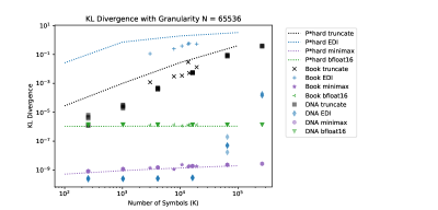
Figure 3: Each compander (or quantization method) is used on random distributions drawn from the prior $P^{*}_{\text{hard}}$. Comparison is given to when each compander is used on the books and DNA datasets.

VI Companding Other Metrics and Spaces

While our primary focus has been KL divergence over the simplex, for context we compare our results to what the same compander analysis would give for other loss functions like squared Euclidean distance ($L_{2}^{2}$) and absolute distance ($L_{1}$ or $TV$ distance). For a vector ${\boldsymbol{x}}$ and its representation $\boldsymbol{z}$ let

$$L_{2}^{2}({\boldsymbol{x}},\boldsymbol{z}) =\sum_{i}(x_{i}-z_{i})^{2}$$ (129)

$$L_{1}({\boldsymbol{x}},\boldsymbol{z}) =\sum_{i}|x_{i}-z_{i}|\,.$$ (130)

For squared Euclidean distance, asymptotic loss was already given by (48) in [2], and scales as $N^{-2}$. It turns out that the maximin single-letter distribution over a bounded interval is the uniform distribution. Thus, the minimax compander for $L_{2}^{2}$ is simply the identity function, i.e. uniform quantization is the minimax for quantizing a hypercube in high-dimensional space under $L_{2}^{2}$ loss. (For unbounded spaces, $L_{2}^{2}$ loss does not scale with $N^{-2}$.)

If we add the expected value constraint to the $L_{2}^{2}$ compander optimization problem, we can derive the best square distance compander for the probability simplex. For alphabet size $K$, we get that the minimax compander for $L_{2}^{2}$ is given by

$$f_{L_{2}^{2},K}(x)=\frac{\sqrt{1+K(K-2)x}-1}{K-2}$$ (131)

and the total $L_{2}^{2}$ loss for probability vector ${\boldsymbol{x}}$ and its quantization $\boldsymbol{z}$ has the relation

$$\lim_{N\to\infty}N^{2}L_{2}^{2}({\boldsymbol{x}},\boldsymbol{z})\leq\frac{1}{3}\,.$$ (132)

For $L_{1}$, unlike KL divergence and $L_{2}^{2}$, the loss scales as $1/N$. Like $L_{2}^{2}$, the minimax single-letter compander for $L_{1}$ loss in the hypercube $[0,1]^{K}$ is the identity function, i.e. uniform quantization. In general, the derivative of the optimal compander for single-letter density $p(x)$ has the form

$$f_{L_{1},K}^{\prime}(x)\,\propto\,\sqrt{p(x)}\,.$$ (133)

On the probability simplex for alphabet size $K$, the worst case prior $p(x)$ has the form

$$p(x)=(\alpha_{K}x+\beta_{K})^{-2}$$ (134)

where $\alpha_{K},\beta_{K}$ are constants scaling to allow $\int_{[0,1]}\,dp=1$ (i.e. $p$ is a valid probability density) and $\int_{[0,1]}x\,dp=1/K$ (i.e. ${\mathbb{E}}_{X\sim p}[X]=1/K$ so $K$ copies of it are expected to sum to $1$).

Thus, the minimax compander on the simplex for $L_{1}$ loss (and letting $\gamma_{K}=\alpha_{K}/\beta_{K}$) satisfies

$$f_{L_{1},K}^{\prime}(x)\, \propto\,(\alpha_{K}x+\beta_{K})^{-1}$$ (135)

$$\implies f_{L_{1},K}(x)\, \propto\,\log((\alpha_{K}/\beta_{K})x+1)$$ (136)

$$\implies f_{L_{1},K}(x) =\frac{\log(\gamma_{K}x+1)}{\log(\gamma_{K}+1)}$$ (137)

since $f_{L_{1},K}(x)$ has to be scaled to go from $0$ to $1$.

The asymptotic $L_{1}$ loss for probability vector ${\boldsymbol{x}}$ and its quantization $\boldsymbol{z}$ is bounded by

$$\lim_{N\to\infty}NL_{1}({\boldsymbol{x}},\boldsymbol{z})=O(\log K)\,.$$ (138)

Loss	Space	Optimal Compander	Asymptotic Upper Bound
KL	Simplex	$f^{*}_{K}(x)=\frac{\mathrm{ArcSinh}(\sqrt{c_{K}(K\log K)\,x})}{\mathrm{ArcSinh}(\sqrt{c_{K}K\log K})}$	$N^{-2}\log^{2}K$
$L_{2}^{2}$	Simplex	$f_{L_{2}^{2},K}(x)=\frac{\sqrt{1+K(K-2)x}-1}{K-2}$	$N^{-2}$
$L_{2}^{2}$	Hypercube	$f_{L_{2}^{2}}(x)=x$ (uniform quantizer)	$N^{-2}K$
$L_{1}\leavevmode\nobreak\ (TV)$	Simplex	$f_{L_{1},K}(x)=\frac{\log(\gamma_{K}x+1)}{\log(\gamma_{K}+1)}$	$N^{-1}\log K$
$L_{1}\leavevmode\nobreak\ (TV)$	Hypercube	$f_{L_{1}}(x)=x$ (uniform quantizer)	$N^{-1}K$

Figure 4: Summary of results for various losses and spaces. Asymptotic Upper Bound is an upper bound on how we expect the loss of the optimal compander to scale with $N$ and $K$ (constant terms are neglected).

VII Connection to Information Distillation

It turns out that the general problem of quantizing the simplex under the average KL divergence loss, as defined in (9), is equivalent to recently introduced problem of information distillation. Information distillation has a number of applications, including in constructing polar codes [21, 22]. In this section we establish this equivalence and also demonstrate how the compander-based solutions to the KL-quantization can lead to rather simple and efficient information distillers.

VII-A Information Distillation

In the information distillation problem we have two random variables $A\in{\mathcal{A}}$ and $B\in{\mathcal{B}}$, where $|{\mathcal{A}}|=K$ (and ${\mathcal{B}}$ can be finite or infinite) under joint distribution $P_{A,B}$ with marginals $P_{A},P_{B}$. The goal is, given some finite $M<|{\mathcal{B}}|$, to find an information distiller (which we will also refer to as a distiller), which is a (deterministic) function $h:{\mathcal{B}}\to[M]$, which minimizes the information loss

$$I(A;B)-I(A;h(B))$$ (139)

associated with quantizing $B\to h(B)$. The interpretation here is that $B$ is a (high-dimensional) noisy observation of some important random variable $A$ and we want to record observation $B$, but only have $\log_{2}M$ bits to do so. Optimal $h$ minimizes the additive loss entailed by this quantization of $B$.

To quantify the amount of loss incurred by this quantization, we use the degrading cost [22, 21]

$$\mathrm{DC}(K,M)=\sup_{P_{A,B}}\inf_{h}I(A;B)-I(A;h(B))\,.$$ (140)

Note that in supremizing over $P_{A,B}$ there is no restriction on ${\mathcal{B}}$, only on $|{\mathcal{A}}|$ and the size of the range of $h$. It has been shown in [22] that there is a $P_{A,B}$ such that

$$\inf_{h}I(A;B)-I(A;h(B))=\Omega(M^{-2/(K-1)})$$ (141)

giving a lower bound to $\mathrm{DC}(K,M)$. For an upper bound, [23] showed that if $2K<M<|{\mathcal{B}}|$, then

$$\mathrm{DC}(K,M)=O(M^{-2/(K-1)})\,.$$ (142)

Specifically, $\mathrm{DC}(K,M)\leq\nu(K)M^{-2/(K-1)}$ where $\nu(K)\approx 16\pi eK^{2}$ for large $K$. While [21] focused on multiplicative loss, their work also implied an improved bound on the additive loss as well; namely, for all $K\geq 2$ and $M^{1/(K-1)}\geq 4$, we have

$$\mathrm{DC}(K,M)\leq 1268(K-1)M^{-2/(K-1)}\,.$$ (143)

VII-B Info Distillation Upper Bounds Via Companders

Using our KL divergence quantization bounds, we will show an upper bound to $\mathrm{DC}(K,M)$ which improves on (143) for $K$ which are not too small and for $M$ which are not exceptionally large. First, we establish the relation between the two problems:

Proposition 8.

For every $P_{A,B}$ define a random variable ${\boldsymbol{X}}\in\triangle_{K-1}$ by setting $X_{a}=P[A=a\,|\,B]$. Then, for every information distiller $h:{\mathcal{B}}\to[M]$ there is a vector quantizer $\boldsymbol{z}:\triangle_{K-1}\to\triangle_{K-1}$ with range of cardinality $M$ such that

$$I(A;B)-I(A;h(B))\geq{\mathbb{E}}[D_{\operatorname{{\scriptscriptstyle KL}}}({\boldsymbol{X}}\|\boldsymbol{z}({\boldsymbol{X}}))]\,.$$ (144)

Conversely, for any vector quantizer $\boldsymbol{z}$ there exists a distiller $h$ such that

$$I(A;B)-I(A;h(B))\leq{\mathbb{E}}[D_{\operatorname{{\scriptscriptstyle KL}}}({\boldsymbol{X}}\|\boldsymbol{z}({\boldsymbol{X}}))]\,.$$ (145)

The inequalities in Proposition 8 can be replaced by equalities if the distiller $h$ and the quantizer $\boldsymbol{z}$ avoid certain trivial inefficiencies. If they do so, there is a clean ‘equivalent’ quantizer $\boldsymbol{z}$ for any distiller $h$, and vice versa, which preserves the expected loss. This equivalence and Proposition 8 are shown in Appendix G.

Thus, we can use KL quantizers to bound the degrading cost above (see Appendix G for details):

$$\mathrm{DC}(K,M) =\sup_{P_{A,B}}\inf_{h}I(A;B)-I(A;h(B))$$ (146)

$$=\sup_{P}\inf_{\boldsymbol{z}}{\mathbb{E}}_{{\boldsymbol{X}}\sim P}[D_{\operatorname{{\scriptscriptstyle KL}}}({\boldsymbol{X}}\|\boldsymbol{Z})]$$ (147)

$$\leq\inf_{\boldsymbol{z}}\sup_{P}{\mathbb{E}}_{{\boldsymbol{X}}\sim P}[D_{\operatorname{{\scriptscriptstyle KL}}}({\boldsymbol{X}}\|\boldsymbol{Z})]\,.$$ (148)

We then use the approximate minimax compander results to give an upper bound to (148). This yields:

Proposition 9.

For any $K\geq 5$ and $M^{1/K}>\lceil 8\log(2\sqrt{K\log K}+1)\rceil$

$$\mathrm{DC}(K,M)\leq\bigg{(}1+18\frac{\log\log K}{\log K}\bigg{)}M^{-\frac{2}{K}}\log^{2}K\,.$$ (149)

Proof.

Consider the right-hand side of (144). The compander-based quantizer from Theorem 4 gives a guaranteed bound on $D({\boldsymbol{X}}\|\boldsymbol{z}({\boldsymbol{X}}))$ (and $M=N^{K}$ substituted), which also holds in expectation. ∎

Remark 12.

Similarly, an upper bound on the divergence covering problem [5, Thm 2] implies

$$\mathrm{DC}(K,M)\leq 800(\log K)M^{-2/(K-1)}\,.$$ (150)

(This appears to be the best known upper bound on $\mathrm{DC}$.) The lower bound on the divergence covering, though, does not imply lower bounds on $\mathrm{DC}$, since divergence covering seeks one collection of $M$ points that are good for quantizing any $P$, whereas $\mathrm{DC}$ permits the collection to depend on $P$. For distortion measures that satisfy the triangle inequality, though, we have a provable relationship between the metric entropy and rate-distortion for the least-favorable prior, see [24, Section 27.7].

VIII Acknowledgements

We would like to thank Anthony Philippakis for his guidance on the DNA $k$-mer experiments.

Appendix Organization

Appendix A

We fill in the details of the proof of Theorem 2.

Appendix B

We prove Proposition 5.

Appendix C

We develop and analyze other types of companders, specifically beta companders, which are optimized to quantize vectors from Dirichlet priors (Section C-A), and power companders, which have the form $f(x)=x^{s}$ and have properties similar to the minimax compander (Section C-B). Supplemental experimental results are also provided.

Appendix D

We analyze the minimax compander and approximate minimax compander more deeply, showing that $c_{K}\in[1/4,3/4]$ (Section D-A) and $\lim_{K\to\infty}c_{K}=1/2$ (Section D-A2), and show that when $c_{K}\approx 1/2$, the approximate minimax compander performs similarly to the minimax compander against all priors $p\in{\mathcal{P}}$ (Section D-B). Supplemental experimental results are also provided.

Appendix E

We prove Theorem 4, showing bounds on the worst-case loss (adversarially selected ${\boldsymbol{x}}$, rather than from a prior) for the power, minimax, and approximate minimax companders.

Appendix G

We discuss the connection to information distillation in detail.

Appendix A Asymptotic Single-Letter Loss Proofs

In this appendix, we give all the proofs necessary for Theorem 2, whose proof outline was discussed in Section IV. We begin with notation in Section A-A. In Section A-B, we give some preliminaries for showing Proposition 6 (which shows that the local loss functions $g_{N}$ converge to the asymptotic local loss function $g$ a.s. when the input $X$ is distributed according to $p\in{\mathcal{P}}$). In Section A-C, we give the proof of Proposition 6. In Section A-D, we give the proof of Proposition 7 (which shows the existence of an integrable $h$ dominating $g_{N}$ when the compander $f$ is from the ‘well-behaved’ set ${\mathcal{F}}^{\dagger}$).

In order to focus on the main ideas, some of the more minor details needed for Proposition 6 and Proposition 7 are omitted and left for later sections. We fill in the details on the lemmas and propositions used in the proof of Proposition 6, including proofs for all results from Section A-B (specifically Lemmas 2 and 3 and Propositions 10, 11 and 12) in Sections A-E, A-F, A-G, A-H and A-I.

We then fill in the details of the lemmas for the proof of Proposition 7, specifically Lemmas 4 and 7.

A-A Notation

Given probability distribution $p$ and interval $I$, $p|_{I}$ denotes $p$ restricted to $I$, i.e. $X\sim p|_{I}$ is the same as $X\sim p$ conditioned on $X\in I$. We also define the probability mass of $I$ under $p$ as $\pi_{p,I}={\mathbb{P}}_{X\sim p}[X\in I]$. If $\pi_{p,I}=0$, we let $p|_{I}$ be uniform on $I$ by default.

Given two probability distributions $p,q$ (over the same domain), their Kolmogorov-Smirnov distance (KS distance) is

$$d_{KS}(p,q)=\|F_{p}-F_{q}\|_{\infty}=\sup_{x}|F_{p}(x)-F_{q}(x)|$$ (151)

(recall that $F_{p},F_{q}$ are the CDFs of $p,q$).

We use standard order-of-growth notation (which are also used in Section II). We review these definitions here for clarity, especially as we will use some of the rarer concepts (in particular, small-$\omega$). For a parameter $t$ and functions $a(t),b(t)$, we say:

$$a(t)=O(b(t)) \iff\limsup_{t\to\infty}|a(t)/b(t)|<\infty$$ (152)

$$a(t)=\Omega(b(t)) \iff\liminf_{t\to\infty}|a(t)/b(t)|>0$$ (153)

$$a(t)=\Theta(b(t)) \iff a(t)=O(b(t)),\,a(t)=\Omega(b(t))\,.$$ (154)

We use small-$o$ notation to denote the strict versions of these:

$$a(t)=o(b(t)) \iff\lim_{t\to\infty}|a(t)/b(t)|=0$$ (155)

$$a(t)=\omega(b(t)) \iff\lim_{t\to\infty}|a(t)/b(t)|=\infty\,.$$ (156)

Sometimes we will want to indicate order-of-growth as $t\to 0$ instead of $t\to\infty$; this will be explicitly mentioned in that case.

A-B Preliminaries for Proposition 6

We first generalize the idea of bins. The bin around $x\in[0,1]$ at granularity $N$ is the interval $I=I^{(n)}$ containing $x$ such that $f(I)=[(n-1)/N,n/N]$ for some $n\in[N]$. This notion relies on integers because $f(I)=[(n-1)/N,n/N]$ for integers $n,N$. We remove the dependence on integers while keeping the basic structure (an interval $I$ about $x$ whose image $f(I)$ is a given size):

Definition 5.

For any $x\in[0,1]$, $\theta\in[0,1]$, and $\varepsilon>0$, we define the pseudo-bin $I^{(x,\theta,\varepsilon)}$ as the interval satisfying:

$$I^{(x,\theta,\varepsilon)} =[x-\theta r^{(x,\theta,\varepsilon)},x+(1-\theta)r^{(x,\theta,\varepsilon)}]\text{ where }$$ (157)

$$r^{(x,\theta,\varepsilon)} =\inf\big{(}r:f(x+(1-\theta)r)-f(x-\theta r)\geq\varepsilon\big{)}\,.$$ (158)

The interpretation of this is that $I^{(x,\theta,\varepsilon)}$ is the minimal interval $x$ such that $|f(I^{(x,\theta,\varepsilon)})|\geq\varepsilon$ and such that $x$ occurs at $\theta$ within $I^{(x,\theta,\varepsilon)}$, i.e. a $\theta$ fraction of $I^{(x,\theta,\varepsilon)}$ falls below $x$ and $1-\theta$ falls above. Its width is $r^{(x,\theta,\varepsilon)}$. This implies that bins are a special type of pseudo-bins. Specifically, for any $x$ and $N$ (and any compander $f$),

$$I^{(n_{N}(x))}=I^{(x,\theta,1/N)}\text{ for some }\theta\in[0,1]\,.$$ (159)

We now consider the size of pseudo-bins as $\varepsilon\to 0$:

Lemma 2.

If $f$ is differentiable at $x$, then

$$\lim_{\varepsilon\to 0}\varepsilon^{-1}r^{(x,\theta,\varepsilon)}=f^{\prime}(x)^{-1}$$ (160)

(including going to $\infty$ when $f^{\prime}(x)=0$). The limit converges uniformly over $\theta\in[0,1]$.

The proof is given in Section A-E. Note that applying this to bins means $\lim_{N\to\infty}Nr^{(n_{N}(x))}=f^{\prime}(x)^{-1}$, and hence when $f^{\prime}(x)>0$ we have $r^{(n_{N}(x))}=N^{-1}f^{\prime}(x)^{-1}+o(N^{-1})$.

For any interval $I$, we want to measure how close $p$ is to uniform over $I$ using the distance measure $d_{KS}(p,q)$ from (151). We will show that when $F^{\prime}_{p}(x)=p(x)$ is well-defined and positive at $x$, $p$ is approximately uniform on any sufficiently small interval $I$ around $x$. Formally:

Proposition 10.

If $p(x)=F^{\prime}_{p}(x)>0$ is well-defined, then for every $\varepsilon>0$ there is a $\delta>0$ such that for all intervals $I$ such that $x\in I$ and $r_{I}\leq\delta$,

$$d_{KS}(p|_{I},{\mathrm{unif}}_{I})\leq\varepsilon\,.$$ (161)

We give the proof in Section A-F. This allows us to use the following:

Proposition 11.

Let $p$ be a probability measure and $I$ be an interval containing $x$ such that $r_{I}\leq x/4$ and $d_{KS}(p|_{I},{\mathrm{unif}}_{I})\leq\varepsilon$ where $\varepsilon\leq 1/2$. Then

$$|\ell_{p,I}-\ell_{{\mathrm{unif}}_{I}}|\leq 2\varepsilon r_{I}^{2}x^{-1}+O(r_{I}^{3}x^{-2})\,.$$ (162)

Recall that $\ell_{p,I}$ is the interval loss of $I$ under distribution $p$ when all points in $I$ are quantized to $\widetilde{y}_{p,I}$, the centroid of the interval. We give the proof of Proposition 11 in Section A-G.

Proposition 12.

For any $x>0$ and any sequence of intervals $I_{1},I_{2},\dots\subseteq[0,1]$ all containing $x$ such that $r_{I_{i}}\to 0$ as $i\to\infty$,

$$\ell_{{\mathrm{unif}}_{I_{i}}}=\frac{1}{24}r_{I_{i}}^{2}x^{-1}+O(r_{I_{i}}^{3}x^{-2})\,.$$ (163)

The proof is in Section A-H.

Note that the above lemmas are all about asymptotic behavior as intervals shrink to $0$ in width; to deal with the (edge) case where they do not, we need the following lemma:

Lemma 3.

For any $I$ such that ${\mathbb{P}}_{X\sim p}[X\in I]>0$, there is some $a_{I}>0$ such that

$$\ell_{p,J}\geq a_{I}\text{ for any }J\supseteq I\,.$$ (164)

We give the proof in Section A-I.

A-C Proof of Proposition 6

We now combine the above results to prove Proposition 6, i.e. that $\lim_{N\to\infty}g_{N}(X)=g(X)$ almost surely when $X\sim p$. Because $p\in{\mathcal{P}}$ (i.e. it is a continuous probability distribution) we will treat the bins as closed sets, i.e. $I^{(n)}=[f(\frac{n-1}{N})^{-1},f(\frac{n}{N})^{-1}]$; this does not affect anything since the resulting overlap is only a finite set of points.

Proof.

Since $p\in{\mathcal{P}}$ then when $X\sim p$ the following hold with probability $1$:

1. $0<X<1$;

2. $f^{\prime}(X)$ is well-defined;

3. $p(X)=F^{\prime}_{p}(X)$ is well defined;

4. $p(X)>0$.

This is because if $p\in{\mathcal{P}}$, and $|S|$ denotes the Lebesgue measure of set $S$, then

$$|S|=0\implies{\mathbb{P}}_{X\sim p}[X\in S]=0\,.$$ (165)

This implies (1) since $\{0,1\}$ is measure-$0$.

Additionally, by Lebesgue’s differentiation theorem for monotone functions, any monotonic function on $[0,1]$ is differentiable almost everywhere on $[0,1]$ (i.e. excluding at most a measure-$0$ set), and compander $f$ and CDF $F_{p}$ are monotonic. This implies 2) and 3). Finally, 4) follows because the set of $X$ such that $p(X)=0$ has probability $0$ under $p$ by definition.

Therefore, we can fix $X\sim p$ and assume it satisfies the above properties.

We now consider the bin size $r_{(n_{N}(X))}$ as $N\to\infty$; there are two cases, (a) $\lim_{N\to\infty}r_{(n_{N}(X))}=0$ and (b) $\limsup_{N\to\infty}r_{(n_{N}(X))}>0$. For case (b), since the length of the interval does not go to zero, $g_{N}(X)=N^{2}\ell_{p,(n_{N}(X))}\to\infty$; additionally, $g(X)=\infty$ by default since case (b) requires that $f^{\prime}(X)=0$, and so $g_{N}(X)\to g(X)$ as we want.

Case (a): In this case (which holds for all $X$ if $f\in{\mathcal{F}}^{\dagger}$), any $\delta>0$ there is some sufficiently large $N^{*}$ (which can depend on $X$) such that

$$N\geq N^{*}\implies r_{(n_{N}(X))}\leq\delta\,.$$ (166)

By Proposition 10, for any $\varepsilon>0$ there is some $\delta>0$ such that for all intervals $I$ where $X\in I$ and $r_{I}\leq\delta$, we have $d_{KS}(p|_{I},{\mathrm{unif}}_{I})\leq\varepsilon$. Putting this together implies that for any $\varepsilon>0$, there is some sufficiently large $N^{*}_{\varepsilon}$ such that for all $N\geq N^{*}_{\varepsilon}$,

$$d_{KS}(p|_{(n_{N}(X))},{\mathrm{unif}}_{(n_{N}(X))})\leq\varepsilon\,.$$ (167)

i.e. $p$ is $\varepsilon$ close to uniform on $I^{(n_{N}(X))}$. Furthermore, we can always choose $\varepsilon\leq 1/2$ and $N^{*}_{\varepsilon}$ sufficiently large that $r_{(n_{N}(X))}\leq X/4$ (since $\lim_{N\to\infty}r_{(n_{N}(X))}=0$). Under these conditions, for $N>N^{*}_{\varepsilon}$ we can apply Proposition 11 and get

$$| \ell_{p,(n_{N}(X))}-\ell_{{\mathrm{unif}}_{(n_{N}(X))}}|$$

$$\leq 2\varepsilon r_{(n_{N}(X))}^{2}X^{-1}+O(r_{(n_{N}(X))}^{3}X^{-2})\,.$$ (168)

We can then turn this around: as $N\to\infty$, we have $\varepsilon\to 0$ and hence $\varepsilon=o(1)$ (as $N\to\infty$), so

$$|\ell_{p,(n_{N}(X))}-\ell_{{\mathrm{unif}}_{(n_{N}(X))}}|=o(r_{(n_{N}(X))}^{2}X^{-1})\,.$$ (169)

We then apply Proposition 12 (note that since $r_{(n_{N}(X))}\leq X/4$ and $X\leq 2\bar{y}_{(n_{N}(X))}$, we know automatically that $r_{(n_{N}(X))}\leq\bar{y}_{(n_{N}(X))}/2$) to get that

$$\ell_{{\mathrm{unif}}_{(n_{N}(X))}}=\frac{1}{24}r_{(n_{N}(X))}^{2}\bar{y}_{(n_{N}(X))}^{-1}+O(r_{(n_{N}(X))}^{3}X^{-2})\,.$$ (170)

However, since $X$ is fixed and $r_{(n_{N}(X))}\to 0$ as $N\to 0$ (and $|X-\bar{y}_{(n_{N}(X))}|\leq r_{(n_{N}(X))}$ since they are both in the bin $I^{(n_{N}(X))}$), we know that $\bar{y}_{(n_{N}(X))}=X(1+o(1))$ where $o(1)$ is in terms of $N$ (as $N\to\infty$). Hence (noting that $(1+o(1))^{-1}$ is still $1+o(1)$ and $O(r_{(n_{N}(X))}^{3}X^{-2})$ is $o(1)r_{(n_{N}(X))}^{2}X^{-1}$) we can re-write the above and combine with (169) to get

$$\ell_{{\mathrm{unif}}_{(n_{N}(X))}} =\frac{1}{24}(1+o(1))r_{(n_{N}(X))}^{2}X^{-1}$$ (171)

$$\implies\ell_{p,(n_{N}(X))} =\frac{1}{24}(1+o(1))r_{(n_{N}(X))}^{2}X^{-1}\,.$$ (172)

We now split things into two cases: (i) $f^{\prime}(X)>0$; (ii) $f^{\prime}(X)=0$.

Case i ($f^{\prime}(X)>0$): For all $N$ there is a $\theta\in[0,1]$ such that $I^{(n_{N}(X))}=I^{(X,\theta,1/N)}$ (bins are pseudo-bins, see Definition 5). Thus, by Lemma 2 (which shows uniform convergence over $\theta$),

$$\lim_{N\to\infty}Nr_{(n_{N}(X))}=f^{\prime}(X)^{-1}\,.$$ (173)

Thus, we may re-write as a little-$o$ and plug into $g_{N}(X)$:

$$r_{(n_{N}(X))} =N^{-1}f^{\prime}(X)^{-1}+o(N^{-1})$$ (174)

$$=N^{-1}f^{\prime}(X)^{-1}(1+o(1))$$ (175)

$$\implies g_{N}(X) =N^{2}\ell_{p,(n_{N}(X))}$$ (176)

$$=N^{2}\frac{1}{24}(1+o(1))r_{(n_{N}(X))}^{2}X^{-1}$$ (177)

$$=N^{2}\frac{1}{24}(1+o(1))N^{-2}f^{\prime}(X)^{-2}X^{-1}$$ (178)

$$=\frac{1}{24}(1+o(1))f^{\prime}(X)^{-2}X^{-1}$$ (179)

implying $\lim_{N\to\infty}g_{N}(X)=g(X)$ as we wanted.

Case ii ($f^{\prime}(X)=0$): As before, for any $N$ there is some $\theta\in[0,1]$ such that $I^{(n_{N}(X))}=I^{(X,\theta,1/N)}$. Thus, by Lemma 2 and as $f^{\prime}(X)=0$, we have

$$\lim_{N\to\infty}Nr_{(n_{N}(X))}=\infty\,.$$ (180)

since the convergence in Lemma 2 is uniform over $\theta$. We can then re-write this as a little-$\omega$:

$$r_{(n_{N}(X))}=\omega(N^{-1})\,.$$ (181)

This implies that

$$g_{N}(X) =N^{2}\ell_{p,(n_{N}(X))}$$ (182)

$$=N^{2}\frac{1}{24}(1+o(1))r_{(n_{N}(X))}^{2}X^{-1}$$ (183)

$$=N^{2}\frac{1}{24}(1+o(1))\omega(N^{-2})X^{-1}$$ (184)

$$=\omega(1)$$ (185)

where $\omega(1)$ means $\lim_{N\to\infty}g_{N}(X)=\infty$. But since $f^{\prime}(X)=0$, by convention we have $g(X)=\frac{1}{24}f^{\prime}(X)^{-2}X^{-1}=\infty$ and so $\lim_{N\to\infty}g_{N}(X)=g(X)$ as we wanted.

Case (b): $\limsup_{N\to\infty}r_{(n_{N}(X))}>0$. Note that this can only happen if $f^{\prime}(X)=0$, so $g(X)=\infty$; hence our goal is to show that $\lim_{N\to\infty}g_{N}(X)=\infty$.

Related to the above, this only happens if $f$ is not strictly monotonic at $X$, i.e. if there is some $a<X$ or some $b>X$ such that $f(X)=f(a)$ or $f(X)=b$ (or both). If both, $[a,b]\subseteq I^{(n_{N}(X))}$ for all $N$. Since $p(X)$ is well-defined and positive, any nonzero-width interval containing $X$ has positive probability mass under $p$. Thus, by Lemma 3, there exists some $\alpha>0$ such that all $J\supseteq[a,b]$ satisfies $\ell_{p,J}\geq\alpha$. But then $g_{N}(X)\geq N^{2}\alpha$ and goes to $\infty$.

If only $a$ exists, we divide the granularities $N$ into two classes: first, $N$ such that $I^{(n_{N}(X))}$ has lower boundary exactly at $X$ (which can happen if $f(X)$ is rational), and second, $N$ such that $I^{(n_{N}(X))}$ has lower boundary below $X$. Call the first class $N^{(1)}(1),N^{(1)}(2),\dots$ and the second $N^{(2)}(1),N^{(2)}(2),\dots$. Then as no $b$ exists, $\lim_{i\to\infty}r^{(n_{N^{(1)}(i)}(X))}=0$, i.e. the bins corresponding to the first class shrink to $0$ and the asymptotic argument applies to them, showing $g_{N^{(1)}(i)}(X)\to\infty$. For the second class, for any $i$, we have $I^{(n_{N^{(2)}(i)}(X))}\supseteq[a,X]$ and so we have an $\alpha>0$ lower bound of the interval loss, and multiplying by $N^{2}$ takes it to $\infty$. Thus since both subsequences of $N$ take $g_{N}(X)$ to $\infty$, we are done. An analogous argument holds if $b$ exists but not $a$.

As this holds for any $X$ under conditions 1-4, which happens almost surely, we are done. ∎

A-D Proof of Proposition 7

To finish our Dominated Convergence Theorem (DCT) argument, we to prove Proposition 7, which gives an integrable function $h$ dominating all the local loss functions $g_{N}$. As with Proposition 6, we do this in stages. We first define:

Definition 6.

For any interval $I$, let

$$\ell^{*}_{I}=\sup_{q}\ell_{q,I}$$ (186)

where $q$ is a probability distribution over $[0,1]$. If $I=I^{(n)}$ we can denote this as $\ell^{*}_{(n)}$.

Since $\ell_{q,I}$ is only affected by $q|_{I}$ (i.e. what $q$ does outside of $I$ is irrelevant), we can restrict $q$ to be a probability distribution over $I$ without affecting the value of $\ell^{*}_{I}$. The question is thus: what is the maximum single-interval loss which can be produced on interval $I$?

Then, we can use the upper bound

$$g_{N}(x)=N^{2}\ell_{p,(n_{N}(x))}\leq N^{2}\ell^{*}_{(n_{N}(x))}\,.$$ (187)

This has the benefit of simplifying the term by removing $p$. We now bound $\ell^{*}_{I}$:

Lemma 4.

For any interval $I$, $\ell^{*}_{I}\leq\frac{1}{2}r_{I}^{2}\bar{y}_{I}^{-1}$.

We give the proof in Section A-J. We can then add the above result to (187) in order to obtain

$$g_{N}(x)\leq N^{2}\ell^{*}_{(n_{N}(x))}\leq N^{2}\frac{1}{2}r_{(n_{N}(x))}^{2}\bar{y}_{(n_{N}(x))}^{-1}\,.$$ (188)

However, it is hard to use this as the boundaries of $I^{(n_{N}(x))}$ in relation to $x$ are inconvenient. Instead, use an interval which is ‘centered’ at $x$ in some way, with the help of the following:

Lemma 5.

If $I\subseteq I^{\prime}$, then $\ell^{*}_{I}\leq\ell^{*}_{I^{\prime}}$.

Proof.

This follows as any $q$ over $I$ is also a distribution over $I^{\prime}$ (giving $0$ probability to $I^{\prime}\backslash I$). ∎

Thus, if we can find some interval $J$ such that $I^{(n_{N}(x))}\subseteq J$ (but of the right size) and which had more convenient boundaries, we can use that instead. We define:

Definition 7.

For compander $f$ at scale $N$ and $x\in[0,1]$, define the interval

$$J^{f,N,x}=f^{-1}\Big{(}\Big{[}f(x)-\frac{1}{N},f(x)+\frac{1}{N}\Big{]}\cap[0,1]\Big{)}\,.$$ (189)

As mentioned, we want this because it contains $I^{(n_{N}(x))}$:

Lemma 6.

For any strictly monotonic $f$ and integer $N$,

$$I^{(n_{N}(x))}\subseteq J^{f,N,x}\,.$$ (190)

Proof.

Since $f$ is strictly monotonic, it has a well-defined inverse $f^{-1}$.

By definition the bin $I^{(n_{N}(x))}$, when passed through the compander $f$, returns $[\frac{n-1}{N},\frac{n}{N}]$, i.e.

$$f(I^{(n_{N}(x))})=\Big{[}\frac{n-1}{N},\frac{n}{N}\Big{]}\,.$$ (191)

Note that this interval has width $1/N$ and includes $f(x)$ and (by definition) it is in $[0,1]$. Hence,

$$f(I^{(n_{N}(x))})\subseteq\Big{[}f(x)-\frac{1}{N},f(x)+\frac{1}{N}\Big{]}\cap[0,1]$$ (192)

$$\implies f(I^{(n_{N}(x))})\subseteq f(J^{f,N,x})$$ (193)

$$\implies I^{(n_{N}(x))}\subseteq J^{f,N,x}$$ (194)

and we are done. ∎

Now we can consider the importance of $f\in{\mathcal{F}}^{\dagger}$: by dominating a monomial $cx^{\alpha}$, we can ‘upper bound’ the interval $J^{f,N,x}$ by the equivalent interval with the compander $f_{*}(x)=cx^{\alpha}$ (i.e. $J^{f,N,x}\subseteq J^{f_{*},N,x}$), which is then much nicer to work with. This also guarantees that $f$ is strictly monotonic.

Lemma 7.

If $f_{1},f_{2}\in{\mathcal{F}}$ are strictly monotonic increasing companders such that $f_{2}-f_{1}$ is also monotonically increasing (not necessarily strictly) and $f_{1}(0)=0$, then for any $x\in[0,1]$ and $N$,

$$J^{f_{2},N,x}\subseteq J^{f_{1},N,x}\,.$$ (195)

The proof is given in Section A-K. Finally, we need a quick lemma concerning the guarantee that if $f\in{\mathcal{F}}^{\dagger}$, the function $g(x)=\frac{1}{24}f^{\prime}(x)^{-2}x^{-1}$ is integrable under any distribution $p$:

Lemma 8.

Let $f\in{\mathcal{F}}^{\dagger}$, and let $g(x)=\frac{1}{24}f^{\prime}(x)^{-2}x^{-1}$. Then for any probability distribution $p$ over $[0,1]$,

$$\int_{[0,1]}g\,dp<\infty\,.$$ (196)

Proof.

If $f\in{\mathcal{F}}^{\dagger}$, then there is some $c>0$ and $\alpha\in(0,1/2]$ such that $f(x)-cx^{\alpha}$ is monotonically increasing. Thus (whenever it is well-defined, which is almost everywhere by Lebesgue’s differentiation theorem for monotone functions) we have $f^{\prime}(x)\geq c\alpha x^{\alpha-1}$ and since $\alpha\in(0,1/2]$, we have $1-2\alpha\geq 0$. Thus, for all $x\in[0,1]$,

$$0\leq g(x)\leq\frac{1}{24}c^{-2}\alpha^{-2}x^{1-2\alpha}\leq\frac{1}{24}c^{-2}\alpha^{-2}$$ (197)

which of course implies that $\int_{[0,1]}g\,p<\infty$. ∎

We can now prove Proposition 7, which will complete the proof of Theorem 2.

Proof of Proposition 7.

As before, let $f_{*}(x)=cx^{\alpha}$; thus $f_{*}(0)=0$ so we can apply Lemma 7. We begin, as outlined in (188), with:

$$g_{N}(x) =N^{2}\ell_{p,(n_{N}(x))}$$ (198)

$$\leq N^{2}\ell^{*}_{(n_{N}(x))}$$ (199)

$$\leq N^{2}\ell^{*}_{J^{f,N,x}}$$ (200)

$$\leq N^{2}\ell^{*}_{J^{f_{*},N,x}}$$ (201)

where (199) follows from the definition of $\ell^{*}_{I}$; (200) follows from Lemmas 5 and 6; and (201) follows from Lemma 7. However, since $f_{*}(x)=cx^{\alpha}$, we have a specific formula we can work with. We have $f^{\prime}_{*}(x)=\alpha cx^{\alpha-1}$ and $f_{*}^{-1}(w)=(w/c)^{1/\alpha}=c^{-1/\alpha}w^{1/\alpha}$. Note that this means we can re-write

$$h(x)=(2^{2/\alpha}+\alpha^{2}2^{1/\alpha-2})f^{\prime}_{*}(x)^{-2}x^{-1}+c^{-1/\alpha}2^{1/\alpha-2}$$ (202)

which sheds some light on the structure of $h(x)$. Using Lemma 8 proves that $\int_{[0,1]}h\,dp$ is finite if $f\in{\mathcal{F}}$, which occurs when $\alpha\leq 1/2$.

Fix a value of $x$. Let $r_{N}(x)$ be the width of $J^{f_{*},N,x}$. We consider two cases: (i) $cx^{\alpha}<1/N$; and (ii) $cx^{\alpha}\geq 1/N$.

Case (i): This implies $f(J^{f_{*},N,x})\subseteq[0,2/N]$ so

$$x <c^{-1/\alpha}N^{-1/\alpha}$$ (203)

$$\implies r_{N}(x) \leq c^{-1/\alpha}(N/2)^{-1/\alpha}\,.$$ (204)

Then, as $J^{f_{*},N,x}$ has lower boundary $0$ in this case, $\bar{y}_{(n_{N}(x))}=r_{N}(x)/2$. Thus, using (188),

$$g_{N}(x) \leq N^{2}\frac{1}{2}r_{N}(x)^{2}\bar{y}_{(n_{N}(x))}^{-1}$$ (205)

$$\leq c^{-1/\alpha}2^{-1/\alpha}N^{-1/\alpha+2}\,.$$ (206)

If $\alpha\leq 1/2$, then $N^{-1/\alpha+2}$ is maximized at $N=1$, and thus

$$g_{N}(x)\leq c^{-1/\alpha}2^{-1/\alpha}\,.$$ (207)

If $\alpha>1/2$, the value $N^{-1/\alpha+2}$ is maximized for the largest possible $N$ still satisfying Case (i). Since $cx^{\alpha}<1/N$, this implies that $N<c^{-1}x^{-\alpha}$. Then,

$$g_{N}(x) \leq c^{-1/\alpha}(c^{-1}x^{-\alpha})^{-1/\alpha+2}2^{-1/\alpha}$$ (208)

$$=c^{-2}x^{1-2\alpha}2^{-1/\alpha}$$ (209)

$$=\alpha^{2}(c\alpha x^{\alpha-1})^{-2}x^{-1}2^{-1/\alpha}$$ (210)

$$=\alpha^{2}f_{*}^{\prime}(x)^{-2}x^{-1}2^{-1/\alpha}\,.$$ (211)

Thus, for Case (i) we have that for any $a\in(0,1]$,

$$g_{N}(x) \leq\alpha^{2}f_{*}^{\prime}(x)^{-2}x^{-1}2^{-1/\alpha}+c^{-1/\alpha}2^{-1/\alpha}\,.$$ (212)

Case (ii): When $cx^{\alpha}\geq 1/N$, since $x\in I\implies\bar{y}_{I}\geq x/2$ (the midpoint of an interval cannot be less than half the largest element of the interval), we can upper-bound $g_{N}(x)$ (using (201) and Lemma 4) by

$$g_{N}(x)\leq N^{2}\frac{1}{2}r_{N}(x)^{2}\bar{y}^{-1}_{J^{f_{*},N,x}}\leq N^{2}r_{N}(x)^{2}x^{-1}\,.$$ (213)

We then bound $r_{N}(x)$ using the Fundamental Theorem of Calculus: since $f$ is monotonically increasing, for any $a\leq b$,

$$\int_{a}^{b}f^{\prime}(t)\,dt\leq f(b)-f(a)$$ (214)

(any discontinuities can only make $f$ increase faster). Additionally $r_{N}(x)=b_{1}-a_{1}$ where $f(b_{1})=\max(f(x)+1/N,1)$ and $f(a_{1})=f(x)-1/N$ (since it’s Case (ii) we know $f(x)-1/N\geq 0$ and since $f\in{\mathcal{F}}^{\dagger}$ is strictly monotonic $a_{1},b_{1}$ are unique). Thus, if we define $a_{2},b_{2}$ such that

$$\int_{a_{2}}^{x}f^{\prime}(t)\,dt=1/N\text{ and }\int_{x}^{b_{2}}f^{\prime}(t)\,dt=1/N$$ (215)

(or $a_{2}=0$ or $b_{2}=1$ if they exceed the $[0,1]$ bounds) we have $r_{N}(x)\leq b_{2}-a_{2}$. Then, because $f-f_{*}$ is monotonically increasing, we can define $a_{3},b_{3}$ where

$$\int_{a_{3}}^{x}f^{\prime}_{*}(t)\,dt=1/N\text{ and }\int_{x}^{b_{3}}f^{\prime}_{*}(t)\,dt=1/N$$ (216)

and get that $r_{N}(x)\leq b_{3}-a_{3}$ (also allowing $b_{3}\geq 1$ if necessary). This yields:

$$r_{N}(x)\leq c^{-1/\alpha}\int_{\max(0,cx^{\alpha}-1/N)}^{\min(1,cx^{\alpha}+1/N)}(f^{-1}_{*})^{\prime}(w)\,dw$$ (217)

$$=c^{-1/\alpha}\int_{\max(0,cx^{\alpha}-1/N)}^{\min(1,cx^{\alpha}+1/N)}\alpha^{-1}w^{1/\alpha-1}\,dw$$ (218)

$$\leq c^{-1/\alpha}\int_{\max(0,cx^{\alpha}-1/N)}^{\min(1,cx^{\alpha}+1/N)}\alpha^{-1}(cx^{\alpha}+1/N)^{1/\alpha-1}\,dw$$ (219)

$$\leq c^{-1/\alpha}\int_{cx^{\alpha}-1/N}^{cx^{\alpha}+1/N}\alpha^{-1}(cx^{\alpha}+1/N)^{1/\alpha-1}\,dw$$ (220)

$$=(2/N)c^{-1/\alpha}\alpha^{-1}(cx^{\alpha}+1/N)^{1/\alpha-1}$$ (221)

$$\implies r_{N}(x) \leq(2/N)c^{-1/\alpha}\alpha^{-1}(cx^{\alpha}+1/N)^{1/\alpha-1}$$ (222)

$$\leq 2N^{-1}c^{-1/\alpha}\alpha^{-1}(2cx^{\alpha})^{1/\alpha-1}$$ (223)

$$=N^{-1}c^{-1/\alpha}\alpha^{-1}2^{1/\alpha}(cx^{\alpha})^{1/\alpha-1}$$ (224)

$$=2^{1/\alpha}N^{-1}\big{(}c^{-1}\alpha^{-1}x^{1-\alpha}\big{)}$$ (225)

$$=2^{1/\alpha}N^{-1}f^{\prime}_{*}(x)^{-1}\,.$$ (226)

Thus, we can incorporate this into our bound (213)

$$g_{N}(x) \leq N^{2}r_{N}(x)^{2}x^{-1}$$ (227)

$$\leq 2^{2/\alpha}f^{\prime}_{*}(x)^{-2}x^{-1}\,.$$ (228)

So, $h(x)$, as the sum of the two cases, upper bounds $g_{N}(x)$ no matter what.

We can also note that if $\alpha\leq 1/2$, then $x^{1-2\alpha}\leq 1$ and hence we can upper-bound $h$ by a constant. Thus $\int_{[0,1]}h\,dp={\mathbb{E}}_{X\sim p}[h(X)]<\infty$ trivially, for any $p$, and we are done. ∎

This completes the proof of (32) in Theorem 2.

A-E Proof of Lemma 2

Proof.

Note that for fixed $\theta$ and $x$, $r^{(x,\theta,\varepsilon)}$ is nonnegative and monotonically decreases as $\varepsilon$ decreases. Thus $\lim_{\varepsilon\to 0}r^{(x,\theta,\varepsilon)}\geq 0$ is well defined.

We first assume that $\lim_{\varepsilon\to 0}r^{(x,\theta,\varepsilon)}=0$ for all $\theta\in[0,1]$. Let $s_{\theta}(r)$ be defined as

$$s_{\theta}(r):=\frac{f(x+(1-\theta)r)-f(x-\theta r)}{r}\,.$$ (229)

We want to show that $\lim_{r\to 0}s_{\theta}(r)=f^{\prime}(x)$ for all $\theta\in[0,1]$, and that this limit is uniform over $\theta\in[0,1]$. For $\theta\in\{0,1\}$ we get respectively the right and left derivatives and since $f$ is differentiable at $x$ we are done for those cases. For $\theta\in(0,1)$ we write:

$$s_{\theta}(r) =\frac{f(x+(1-\theta)r)-f(x-\theta r)}{r}$$ (230)

$$=\frac{f(x+(1-\theta)r)-f(x)}{r}$$

$$\quad\quad+\frac{f(x)-f(x-\theta r)}{r}$$ (231)

$$=(1-\theta)\frac{f(x+(1-\theta)r)-f(x)}{(1-\theta)r}$$

$$\quad\quad+\theta\frac{f(x-\theta r)-f(x)}{-\theta r}\,.$$ (232)

This implies

$$\lim_{r\to 0}s_{\theta}(r) =\lim_{r\to 0}\bigg{(}(1-\theta)\frac{f(x+(1-\theta)r)-f(x)}{(1-\theta)r}$$

$$\quad\quad+\theta\frac{f(x-\theta r)-f(x)}{-\theta r}\bigg{)}$$ (233)

$$=(1-\theta)f^{\prime}(x)+\theta f^{\prime}(x)=f^{\prime}(x)\,.$$ (234)

Furthermore we note that the convergence is uniform over $\theta\in[0,1]$. This is because for any $\alpha>0$, there is a $\delta>0$ such that for $|r|\leq\delta$,

$$\bigg{|}\frac{f(x+r)-f(x)}{r}-f^{\prime}(x)\bigg{|}\leq\alpha\,.$$ (235)

But $|r|\leq\delta\implies|-\theta r|\leq\delta$ and $|(1-\theta)r|\leq\delta$. Thus,

$$|s_{\theta}(r)-f^{\prime}(x)|$$

$$=\bigg{|}(1-\theta)\frac{f(x+(1-\theta)r)-f(x)}{(1-\theta)r}$$

$$\quad\quad+\theta\frac{f(x-\theta r)-f(x)}{-\theta r}-f^{\prime}(x)\bigg{|}$$ (236)

$$\leq\bigg{|}(1-\theta)\frac{f(x+(1-\theta)r)-f(x)}{(1-\theta)r}-(1-\theta)f^{\prime}(x)\bigg{|}$$

$$\quad\quad+\bigg{|}\theta\frac{f(x-\theta r)-f(x)}{-\theta r}-\theta f^{\prime}(x)\bigg{|}$$ (237)

$$\leq(1-\theta)\alpha+\theta\alpha$$ (238)

$$=\alpha\,.$$ (239)

Thus we have uniform convergence of $s_{\theta}(r)$ to $f^{\prime}(x)$ over all $\theta\in[0,1]$ as $r\to 0$. Since $r^{(x,\theta,\varepsilon)}\to 0$ as $\varepsilon\to 0$,

$$f^{\prime}(x) =\lim_{\varepsilon\to 0}s_{\theta}(r^{(x,\theta,\varepsilon)})$$ (240)

$$=\lim_{\varepsilon\to 0}\frac{f(x+(1-\theta)r^{(x,\theta,\varepsilon)})-f(x-\theta r^{(x,\theta,\varepsilon)})}{r^{(x,\theta,\varepsilon)}}$$ (241)

$$=\lim_{\varepsilon\to 0}\frac{\varepsilon}{r^{(x,\theta,\varepsilon)}}$$ (242)

$$\implies\lim_{\varepsilon\to 0}\varepsilon^{-1}\,r^{(x,\theta,\varepsilon)}=f^{\prime}(x)^{-1}$$ (243)

as we wanted. The third equality comes from the definition of $r^{(x,\theta,\varepsilon)}$ (158) and the fact that $f^{\prime}(x)$ is well-defined.

Now we need to consider what happens if $\lim_{\varepsilon\to 0}r^{(x,\theta,\varepsilon)}\neq 0$ for some values of $\theta$; this can either be because the limit is positive or because the limit does not exist, but in either case it is clearly only possible if $f$ is not strictly monotonic at $x$ and hence only if $f^{\prime}(x)=0$. Additionally, it can only happen if $f$ is flat at $x$, i.e. there is either some $a<x$ or some $a>x$ such that $f(a)=f(x)$ (or both). In this case, for any $0<\theta<1$, $I^{(x,\theta,\varepsilon)}$ contains the interval between $a$ and $x$ and hence $r^{(x,\theta,\varepsilon)}\geq|x-a|$. For $\theta=0$ and $\theta=1$, either $r^{(x,\theta,\varepsilon)}$ is bounded away from $0$, or it approaches $0$; in the first case, $\varepsilon^{-1}r^{(x,\theta,\varepsilon)}\to\infty$ by default, while in the second the proof for the $\lim_{\varepsilon\to 0}r^{(x,\theta,\varepsilon)}=0$ case holds.

Thus, for all values of $\theta\in[0,1]$, we know that $\lim_{\varepsilon\to 0}\varepsilon^{-1}r^{(x,\theta,\varepsilon)}=\infty$ as we need; and this is uniform over $\theta$ because for any $\theta\in(0,1)$ we have $\varepsilon^{-1}r^{(x,\theta,\varepsilon)}\geq\varepsilon^{-1}|x-a|$, meaning that for any large $\alpha>0$, we can choose $\varepsilon^{*}$ small enough so that for all $\varepsilon<\varepsilon^{*}$ all of the following hold: (i) $\varepsilon^{-1}|x-a|>\alpha$; (ii) $\varepsilon^{-1}r^{(x,0,\varepsilon)}>\alpha$; and (iii) $\varepsilon^{-1}r^{(x,0,\varepsilon)}>\alpha$. Thus, we have uniform convergence and we are done. ∎

A-F Proof of Proposition 10

Proof.

We can assume that $\varepsilon\leq 1/2$ (if not, just use the value of $\delta$ corresponding to $\varepsilon=1/2$). Let $\delta>0$ be such that for all $x^{\prime}$ such that $|x^{\prime}-x|\leq\delta$,

$$\Big{|}\frac{F_{p}(x^{\prime})-F_{p}(x)}{x^{\prime}-x}-p(x)\Big{|}\leq p(x)\varepsilon/8\,.$$ (244)

Since the derivative $p(x)=F^{\prime}_{p}(x)$ is well-defined, this $\delta$ must exist. Then for $x^{\prime}\in I$,

$$\big{|}(F_{p}(x^{\prime})-F_{p}(x))-(x^{\prime}-x)p(x)\big{|}$$

$$\quad\quad\leq|x^{\prime}-x|p(x)\varepsilon/8\leq r_{I}p(x)\varepsilon/8\,.$$ (245)

Now let $x^{\prime\prime}$ also be such that $|x^{\prime\prime}-x|\leq\delta$. Then

$$\big{|}(F_{p}(x^{\prime\prime}) -F_{p}(x^{\prime}))-(x^{\prime\prime}-x^{\prime})p(x)\big{|}$$ (246)

$$=\big{|}((F_{p}(x^{\prime\prime})-F_{p}(x))-(x^{\prime\prime}-x)p(x))$$

$$\quad\quad-\leavevmode\nobreak\ ((F_{p}(x^{\prime})-F_{p}(x))-(x^{\prime}-x)p(x))\big{|}$$ (247)

$$\leq r_{I}p(x)\varepsilon/4\,.$$ (248)

Let $x^{\prime}$ be the lower boundary of $I$, so $x^{\prime}+r_{I}$ is the upper boundary of $I$ (for which the above of course applies). Then we get

$$\big{|}(F_{p}(x^{\prime}+r_{I})-F_{p}(x^{\prime}))-r_{I}p(x)\big{|} \leq r_{I}p(x)\varepsilon/4$$ (249)

$$\implies\Big{|}\frac{F_{p}(x^{\prime}+r_{I})-F_{p}(x^{\prime})}{r_{I}p(x)}-1\Big{|} \leq\varepsilon/4\,.$$ (250)

Then we know that for any $x^{\prime\prime}\in I$,

$$F_{p|_{I}}(x^{\prime\prime})=\frac{F_{p}(x^{\prime\prime})-F_{p}(x^{\prime})}{F_{p}(x^{\prime}+r_{I})-F_{p}(x^{\prime})}\,.$$ (251)

By (248) we know that

$$(x^{\prime\prime}-x^{\prime})p(x)- r_{I}p(x)\varepsilon/4\leq F_{p}(x^{\prime\prime})-F_{p}(x^{\prime})$$

$$\leq(x^{\prime\prime}-x^{\prime})p(x)+r_{I}p(x)\varepsilon/4$$ (252)

$$\implies r_{I}p(x)((x^{\prime\prime}-x^{\prime}) /r_{I}-\varepsilon/4)\leq F_{p}(x^{\prime\prime})-F_{p}(x^{\prime})$$

$$\leq r_{I}p(x)((x^{\prime\prime}-x^{\prime})/r_{I}+\varepsilon/4)$$ (253)

and by (250) we know that

$$r_{I}p(x)-r_{I}p(x)\varepsilon/4 \leq F_{p}(x+r_{I})-F_{p}(x^{\prime})$$

$$\leq r_{I}p(x)+r_{I}p(x)\varepsilon/4$$ (254)

$$\implies r_{I}p(x)(1-\varepsilon/4) \leq F_{p}(x+r_{I})-F_{p}(x^{\prime})$$

$$\leq r_{I}p(x)(1+\varepsilon/4)\,.$$ (255)

Noting that $(x^{\prime\prime}-x^{\prime})/r_{I}=F_{{\mathrm{unif}}_{I}}(x^{\prime\prime})\in[0,1]$ is the CDF of the uniform distribution on $I$, we get that

$$F_{p|_{I}}(x^{\prime\prime}) \geq\frac{r_{I}p(x)((x^{\prime\prime}-x^{\prime})/r_{I}-\varepsilon/4)}{r_{I}p(x)(1+\varepsilon/4)}$$ (256)

$$=\frac{(x^{\prime\prime}-x^{\prime})/r_{I}-\varepsilon/4}{1+\varepsilon/4}$$ (257)

$$\geq F_{{\mathrm{unif}}_{I}}(x^{\prime\prime})-\varepsilon$$ (258)

and similarly that

$$F_{p|_{I}}(x^{\prime\prime}) \leq\frac{r_{I}p(x)((x^{\prime\prime}+x^{\prime})/r_{I}-\varepsilon/4)}{r_{I}p(x)(1-\varepsilon/4)}$$ (259)

$$=\frac{(x^{\prime\prime}-x^{\prime})/r_{I}+\varepsilon/4}{1-\varepsilon/4}$$ (260)

$$\leq F_{{\mathrm{unif}}_{I}}(x^{\prime\prime})+\varepsilon$$ (261)

and hence for such a $\delta>0$ we have for all $I$ containing $x$ and such that $r_{I}\leq\delta$ we have

$$|F_{p|_{I}}(x^{\prime\prime})-F_{{\mathrm{unif}}_{I}}(x^{\prime\prime})|\leq\varepsilon$$ (262)

for all $x^{\prime\prime}\in I$. For $x^{\prime\prime}\not\in I=[x^{\prime},x^{\prime}+r_{I}]$ we then observe that

$$F_{p|_{I}}(x^{\prime\prime})=F_{{\mathrm{unif}}_{I}}(x^{\prime\prime})=\begin{cases}0&\text{if }x^{\prime\prime}<x^{\prime}\\ 1&\text{if }x^{\prime\prime}>x^{\prime}+r_{I}\end{cases}$$ (263)

thus finishing the proof. ∎

A-G Proof of Proposition 11

Proof.

Let $\xi=\widetilde{y}_{p,I}-\bar{y}_{I}$. Then:

$$|\xi| =\bigg{|}\int_{I}\big{(}{\mathbb{P}}_{X\sim p|_{I}}[X\geq x]-{\mathbb{P}}_{X\sim{\mathrm{unif}}_{I}}[X\geq x]\big{)}\,dx\bigg{|}$$ (264)

$$\leq\int_{I}\big{|}{\mathbb{P}}_{X\sim p|_{I}}[X\geq x]-{\mathbb{P}}_{X\sim{\mathrm{unif}}_{I}}[X\geq x]\big{|}\,dx$$ (265)

$$\leq r_{I}\varepsilon\,.$$ (266)

For any distribution $q$ and any fixed value $w$, define the shift operator $T_{w}(q)$ to denote the distribution of $X-w$ where $X\sim q$ (i.e. just shift it by $w$). Note that $T_{\widetilde{y}_{p,I}}(p|_{I})$ and $T_{\bar{y}_{I}}({\mathrm{unif}}_{I})$ are both constructed to have expectation $0$, and in particular $T_{\bar{y}_{I}}({\mathrm{unif}}_{I})$ is the uniform distribution over an interval of width $r_{I}$ centered at $0$. Additionally,

$$d_{KS} (T_{\widetilde{y}_{p,I}}(p|_{I}),T_{\bar{y}_{I}}({\mathrm{unif}}_{I}))$$ (267)

$$\leq d_{KS}(T_{\widetilde{y}_{p,I}}(p|_{I}),T_{\widetilde{y}_{p,I}}({\mathrm{unif}}_{I}))$$ (268)

$$\leavevmode\nobreak\ \leavevmode\nobreak\ \leavevmode\nobreak\ \leavevmode\nobreak\ +d_{KS}(T_{\widetilde{y}_{p,I}}({\mathrm{unif}}_{I}),T_{\bar{y}_{I}}({\mathrm{unif}}_{I}))$$ (269)

$$\leq 2\varepsilon$$ (270)

since $d_{KS}(\cdot,\cdot)$ is a metric, $d_{KS}(q_{1},q_{2})=d_{KS}(T_{w}(q_{1}),T_{w}(q_{2}))$ for any $q_{1},q_{2}$ and $w$, and

$$d_{KS}(T_{z_{1}}({\mathrm{unif}}_{I}),T_{z_{2}}({\mathrm{unif}}_{I}))\leq|z_{2}-z_{1}|/r_{I}\,.$$ (271)

For convenience, let $q_{1}=T_{\widetilde{y}_{p,I}}(p|_{I})$ and $q_{2}=T_{\bar{y}_{I}}({\mathrm{unif}}_{I})$, and let $W_{1}\sim q_{1}$ and $W_{2}\sim q_{2}$. We know the following: ${\mathbb{E}}[W_{1}]={\mathbb{E}}[W_{2}]=0$; $d_{KS}(q_{1},q_{2})\leq 2\varepsilon$; and $q_{1},q_{2}$ have support on $[-r_{I},r_{I}]$.

Let $\eta_{i}={\mathbb{E}}[W_{1}^{i}]-{\mathbb{E}}[W_{2}^{i}]$. Then we can compute the following:

$$|\eta_{i}| =\bigg{|}\int_{0}^{r_{I}^{i}}({\mathbb{P}}[W_{1}^{i}\geq x]-{\mathbb{P}}[W_{2}^{i}\geq x])\,dx$$

$$\quad\quad-\int_{0}^{r_{I}^{i}}({\mathbb{P}}[W_{1}^{i}\leq-x]-{\mathbb{P}}[W_{2}^{i}\leq-x])\,dx\bigg{|}\,.$$ (272)

If $i$ is odd, then we do a $u$-substitution with $u=x^{1/i}$ and get

$$|\eta_{i}| =\bigg{|}\int_{0}^{r_{I}^{i}}({\mathbb{P}}[W_{1}\geq x^{1/i}]-{\mathbb{P}}[W_{2}\geq x^{1/i}])\,dx$$

$$\quad\quad-\int_{-r_{I}^{i}}^{0}({\mathbb{P}}[W_{1}\leq-x^{1/i}]-{\mathbb{P}}[W_{2}^{i}\leq-x^{1/i}])\,dx\bigg{|}$$ (273)

$$=i\,\bigg{|}\int_{0}^{r_{I}}u^{i-1}({\mathbb{P}}[W_{1}\geq u]-{\mathbb{P}}[W_{2}\geq u])\,du$$

$$\quad\quad-\int_{-r_{I}}^{0}u^{i-1}({\mathbb{P}}[W_{1}\leq u]-{\mathbb{P}}[W_{2}\leq u])\,du\bigg{|}$$ (274)

$$\leq 2\int_{0}^{r_{I}}iu^{i-1}2\varepsilon du=4\varepsilon r_{I}^{i}\,.$$ (275)

Similarly if $i$ is even we get

$$|\eta_{i}| =\bigg{|}\int_{0}^{r_{I}^{i}}({\mathbb{P}}[W_{1}\geq x^{1/i}]-{\mathbb{P}}[W_{2}\geq x^{1/i}])\,dx$$

$$\quad\quad+\int_{-r_{I}^{i}}^{0}({\mathbb{P}}[W_{1}\leq-x^{1/i}]-{\mathbb{P}}[W_{2}^{i}\leq-x^{1/i}])\,dx\bigg{|}$$ (276)

$$=i\,\bigg{|}\int_{0}^{r_{I}}u^{i-1}({\mathbb{P}}[W_{1}\geq u]-{\mathbb{P}}[W_{2}\geq u])\,du$$

$$\quad\quad+\int_{-r_{I}}^{0}u^{i-1}({\mathbb{P}}[W_{1}\leq u]-{\mathbb{P}}[W_{2}\leq u])\,du\bigg{|}$$ (277)

$$\leq 2\int_{0}^{r_{I}}iu^{i-1}2\varepsilon du=4\varepsilon r_{I}^{i}$$ (278)

and we can conclude that $|\eta_{i}|\leq 4\varepsilon r_{I}^{i}$ in general.

Then we can take the respective Taylor expansions: let $X_{1}\sim p|_{I}$ and $X_{2}\sim{\mathrm{unif}}_{I}$ (and $W_{1}\sim q_{1},W_{2}\sim q_{2}$ as above). We get

$$\ell_{p,I} ={\mathbb{E}}[X_{1}\log(X_{1}/\widetilde{y}_{p,I})]$$ (279)

$$=\widetilde{y}_{p,I}{\mathbb{E}}[(W_{1}/\widetilde{y}_{p,I}+1)\log(W_{1}/\widetilde{y}_{p,I}+1)]$$ (280)

$$=\widetilde{y}_{p,I}{\mathbb{E}}\left[W_{1}/\widetilde{y}_{p,I}+\frac{(W_{1}/\widetilde{y}_{p,I})^{2}}{2}-\frac{(W_{1}/\widetilde{y}_{p,I})^{3}}{6(1+\eta)^{2}}\right]$$ (281)

where $\eta$ is a number between $0$ and $W_{1}/\widetilde{y}_{p,I}$ (we get this using Lagrange’s formula for the error).

Since $W_{1}+\widetilde{y}_{p,I}\in I$, we know that

$$\widetilde{y}_{p,I}-r_{I}\leq w+\widetilde{y}_{p,I}\leq\widetilde{y}_{p,I}+r_{I}\,.$$ (282)

Since $r_{I}<x/4$ and $\widetilde{y}_{p,I}\geq x-r_{I}$ (as $x,\widetilde{y}_{p,I}$ share the width-$r_{I}$ interval $I$), we get that $\widetilde{y}_{p,I}>3r_{I}$, and therefore

$$\frac{2}{3}\widetilde{y}_{p,I} <W_{1}+\widetilde{y}_{p,I}<\frac{4}{3}\widetilde{y}_{p,I}$$ (283)

$$\implies\frac{-1}{3} <W_{1}/\widetilde{y}_{p,I}<\frac{1}{3}\,.$$ (284)

This gives that $|\eta|<1/3$. Using this and the fact that ${\mathbb{E}}[W_{1}]=0$ by construction, we can write (281) as

$$\ell_{p,I} \leq\frac{1}{2}{\mathbb{E}}[W_{1}^{2}]/\widetilde{y}_{p,I}+\frac{|{\mathbb{E}}[W_{1}^{3}]|}{8/3}(\widetilde{y}_{p,I})^{-2}$$ (285)

$$\leq\frac{1}{2}{\mathbb{E}}[W_{1}^{2}]/\widetilde{y}_{p,I}+\frac{r_{I}^{3}}{8/3(x-r_{I})^{2}}\,.$$ (286)

Since $r_{I}<x/4$, we know that $x-r_{I}>(3/4)x$, and hence

$$\ell_{p,I} \leq\frac{1}{2}{\mathbb{E}}[W_{1}^{2}]/\widetilde{y}_{p,I}+(2/3)r_{I}^{3}x^{-2}\,.$$ (287)

Hence we get

$$\ell_{p,I} =\frac{1}{2}{\mathbb{E}}[W_{1}^{2}]/\widetilde{y}_{p,I}+O(r_{I}^{3}x^{-2})\,.$$ (288)

Because $x-r_{I}\leq\bar{y}_{I}$ as well (and $W_{2}$ has support on $[-r_{I},r_{I}]$) we can repeat the above arguments to conclude similarly that

$$\ell_{{\mathrm{unif}}_{I}}=\frac{1}{2}{\mathbb{E}}[W_{2}^{2}]/\bar{y}_{I}+O(r_{I}^{3}x^{-2})\,.$$ (289)

Hence their difference is

$$|\ell_{p,I}-\ell_{{\mathrm{unif}}_{I}}|\leq$$ (290)

$$\frac{1}{2}\big{|}{\mathbb{E}}[W_{1}^{2}]/\widetilde{y}_{p,I}-{\mathbb{E}}[W_{2}^{2}]/\bar{y}_{I}\big{|}+O(r_{I}^{3}x^{-2})\,.$$ (291)

Taking the main term, we split it into three parts:

$$\big{|}{\mathbb{E}} [W_{1}^{2}]/\widetilde{y}_{p,I}-{\mathbb{E}}[W_{2}^{2}]/\bar{y}_{I}\big{|}$$ (292)

$$\leq\big{|}{\mathbb{E}}[W_{1}^{2}]/\widetilde{y}_{p,I}-{\mathbb{E}}[W_{1}^{2}]/x\big{|}$$ (293)

$$\leavevmode\nobreak\ \leavevmode\nobreak\ +\big{|}{\mathbb{E}}[W_{2}^{2}]/\bar{y}_{I}-{\mathbb{E}}[W_{2}^{2}]/x\big{|}$$ (294)

$$\leavevmode\nobreak\ \leavevmode\nobreak\ +\big{|}{\mathbb{E}}[W_{1}^{2}]/x-{\mathbb{E}}[W_{2}^{2}]/x\big{|}\,.$$ (295)

The first part (293) can be bounded by

$$\big{|}{\mathbb{E}}[W_{1}^{2}]/\widetilde{y}_{p,I}-{\mathbb{E}}[W_{1}^{2}]/x\big{|} \leq|{\mathbb{E}}[W_{1}^{2}]|\,|1/\widetilde{y}_{p,I}-1/x|$$ (296)

$$\leq r_{I}^{2}\frac{|x-\widetilde{y}_{p,I}|}{\widetilde{y}_{p,I}x}$$ (297)

$$\leq(4/3)r_{I}^{3}x^{-2}$$ (298)

$$=O(r_{I}^{3}x^{-2})\,.$$ (299)

An analogous argument bounds (294), giving

$$\big{|}{\mathbb{E}}[W_{2}^{2}]/\bar{y}_{I}-{\mathbb{E}}[W_{2}^{2}]/x\big{|}=O(r_{I}^{3}x^{-2})\,.$$ (300)

Finally, (295) follows from

$$\big{|}{\mathbb{E}}[W_{1}^{2}]/x-{\mathbb{E}}[W_{2}^{2}]/x\big{|}=|\eta_{2}|x^{-1}\leq 4\varepsilon r_{I}^{2}x^{-1}\,.$$ (301)

Thus, plugging it all into (291) we get

$$|\ell_{p,I}-\ell_{{\mathrm{unif}}_{I}}|\leq 2\varepsilon r_{I}^{2}x^{-1}+O(r_{I}^{3}x^{-2})\,.$$ (302)

∎

A-H Proof of Proposition 12

Proof.

Let $i^{*}$ be such that $r_{I_{i^{*}}}\leq x/4$ for all $i\geq i^{*}$ (since $\lim_{i\to\infty}r_{I_{i}}=0$ this exists) and WLOG consider the sequence of $i\geq i^{*}$. The result then follows from the Taylor series of $\ell_{{\mathrm{unif}}_{I_{i}}}$, as shown by (289) (see proof of Proposition 11 in Section A-G). Keeping the definition from the proof of Proposition 11, we let $W_{2}\sim T_{\bar{y}_{I_{i}}}({\mathrm{unif}}_{I_{i}})$, i.e. uniform over a width-$r_{I_{i}}$ interval centered at $0$. Thus we have ${\mathbb{E}}[W_{2}^{2}]=\frac{1}{12}r_{I_{i}}^{2}$ and hence (289) yields

$$\ell_{{\mathrm{unif}}_{I_{i}}} =\frac{1}{2}{\mathbb{E}}[W_{2}^{2}]/\bar{y}_{I_{i}}+O(r_{I}^{3}x^{-2})$$ (303)

$$=\frac{1}{24}r_{I_{i}}^{2}\bar{y}_{I_{i}}^{-1}+O(r_{I_{i}}^{3}x^{-2})\,.$$ (304)

But $\bar{y}_{I_{i}}$ and $x$ share the interval $I_{i}$ and hence as $r_{I_{i}}\to 0$,

$$\bar{y}_{I_{i}} =x+O(r_{I_{i}})$$ (305)

$$=x(1+O(r_{I_{i}}x^{-1}))$$ (306)

$$\implies\bar{y}_{I_{i}}^{-1} =x^{-1}(1+O(r_{I_{i}}x^{-1}))$$ (307)

since when $r_{I_{i}}$ is very small, $O(r_{I_{i}}x^{-1})$ is very small so $(1+O(r_{I_{i}}x^{-1})^{-1}=1+O(r_{I_{i}}x^{-1})$ (the inverse of a value close to $1$ is also close to $1$). Thus, we can replace $\bar{y}_{I_{i}}^{-1}$ in (304) to get

$$\ell_{{\mathrm{unif}}_{I}}=\frac{1}{24}r_{I_{i}}^{2}x^{-1}+O(r_{I_{i}}^{3}x^{-2})$$ (308)

as we wanted. ∎

A-I Single-Interval Loss Function Properties and Proof of Lemma 3

We prove Lemma 3 here; to do so, we show a few lemmas concerning the single-interval loss function $\ell_{p,I}$. First, we show an alternative formula for $\ell_{p,I}$ which sheds some light on it:

Lemma 9.

For any $p,I$,

$$\ell_{p,I}={\mathbb{E}}_{X\sim p|_{I}}[X\log X]-\widetilde{y}_{p,I}\log(\widetilde{y}_{p,I})\,.$$ (309)

Proof.

We compute $\ell_{p,I}$ as follows:

$$\ell_{p,I} ={\mathbb{E}}_{X\sim p}[X\log(X/\widetilde{y}_{p,I})\,|\,X\in I]$$ (310)

$$={\mathbb{E}}_{X\sim p|_{I}}[X\log(X/\widetilde{y}_{p,I})]$$ (311)

$$={\mathbb{E}}_{X\sim p|_{I}}[X\log(X)-X\log(\widetilde{y}_{p,I})]$$ (312)

$$={\mathbb{E}}_{X\sim p|_{I}}[X\log X]-{\mathbb{E}}_{X\sim p|_{I}}[X]\log(\widetilde{y}_{p,I})$$ (313)

$$={\mathbb{E}}_{X\sim p|_{I}}[X\log X]-\widetilde{y}_{p,I}\log(\widetilde{y}_{p,I})$$ (314)

since $\widetilde{y}_{p,I}={\mathbb{E}}_{X\sim p|_{I}}[X]$. ∎

We now want to show that it really does represent something resembling a loss function: first, that it is nonnegative, and second that it achieves equality if and only if $X\sim p$ on $I$ is known for sure (so the decoded value can be guaranteed to equal $X$).

Lemma 10.

For any $p$ and $I\subseteq[0,1]$ (even $p$ is not continuous),

$$\ell_{p,I}\geq 0$$ (315)

with equality if and only if there is some $w\in I$ s.t.

$${\mathbb{P}}_{X\sim p}[X=w\,|\,X\in I]=1\,.$$ (316)

Proof.

Using Lemma 9, if we define the function $h(t)=t\log t$ then since $h$ is strictly convex, by Jensen’s Inequality (where all expectations are over $X\sim p|_{I}$)

$$\ell_{p,I}={\mathbb{E}}[h(X)]-h({\mathbb{E}}[X])\geq 0$$ (317)

with equality if and only if $X\sim p|_{I}$ is fixed with probability $1$. ∎

This yields the following corollary:

Corollary 2.

If $p\in{\mathcal{P}}$ and $I$ has nonzero width,

$$\ell_{p,I}>0\,.$$ (318)

This follows because $p\in{\mathcal{P}}$ is continuous and so cannot have all its mass on a particular value in any nonzero-width $I$. If $I$ has zero probability mass under $p$, then $\ell_{p,I}$ defaults to the interval loss under a uniform distribution.

Finally, we can prove Lemma 3. Recall that it shows that if $I$ has nonzero probability mass under $p$, one cannot get the interval loss to approach $0$ by choosing $J\supseteq I$, i.e. if $p\in{\mathcal{P}}$ and $I$ is such that ${\mathbb{P}}_{X\sim p}[X\in I]>0$, then there is some $\alpha>0$ (which can depend on $I$) such that

$$\ell_{p,J}\geq\alpha\text{ for all }J\supseteq I\,.$$ (319)

Proof of Lemma 3.

We can re-write $\ell_{p,J}$ as

$$\ell_{p,J} ={\mathbb{E}}_{X\sim p}[X\log(X/\widetilde{y}_{p,J})\,|\,X\in J]$$ (320)

$$=\int_{J}\frac{p(x)}{\int_{J}dp}x\log(x/\widetilde{y}_{p,J})\,dx$$ (321)

where $\int_{J}\,dp$ is just the integral representation of ${\mathbb{P}}_{X\sim p}[X\in J]$.

Therefore, since $p\in{\mathcal{P}}$, $\ell_{p,J}$ is continuous at $J$ with respect to the boundaries of $J$ (the inverse probability mass $(\int_{J}dp)^{-1}$ is continuous since $\int_{J}dp\geq\int_{I}dp>0$).

Thus, we can consider $\ell_{p,J}$ as a continuous function over the boundaries of $J$ on the domain where $I\subseteq J\subseteq[0,1]$; this domain can be represented as a closed subset of $[0,1]^{2}$ and hence is compact. Thus, by the Weierstrass extreme value theorem, $\ell_{J,p}$ achieves its minimum $\alpha$ on this domain, and by Corollary 2 it must be positive.

Hence, we have shown that there is an $\alpha>0$ such that for any $J\supseteq I$, $\ell_{p,J}>\alpha$. ∎

A-J Proof of Lemma 4

Proof.

We WLOG restrict ourselves to $q$ which are probability distributions over $I$. Let ${\mathcal{P}}_{I}$ denote the set of probability distributions over $I$ (not necessarily continuous) and ${\mathcal{P}}^{\prime}_{I}$ denote the set of probability distributions over $I$ which place all the probability mass on the boundaries $\bar{y}_{I}-r_{I}/2$ and $\bar{y}_{I}+r_{I}/2$, i.e. for all $q^{\prime}\in{\mathcal{P}}^{\prime}_{I}$ we have

$${\mathbb{P}}_{X\sim q^{\prime}}[X\in\{\bar{y}_{I}-r_{I}/2,\bar{y}_{I}+r_{I}/2\}]=1\,.$$ (322)

We then make the following claim:

Claim 1: For all $q\in{\mathcal{P}}_{I}$, exists $q^{\prime}\in{\mathcal{P}}^{\prime}_{I}$ such that $\ell_{q,I}\leq\ell_{q^{\prime},I}$.

This follows from the convexity of the function $x\log(x)$ and the definition of $\ell_{q,I}$, i.e.

$$\ell_{q,I}={\mathbb{E}}_{X\sim q}[X\log(X/\widetilde{y}_{q,I})]$$ (323)

(since $q$ in this case is a distribution over $I$, we removed the condition $X\in I$ as it is redundant). In particular, if $q^{\prime}$ is the (unique) distribution in ${\mathcal{P}}^{\prime}_{I}$ such that ${\mathbb{E}}_{X\sim q^{\prime}}[X]=\widetilde{y}_{q,I}$ (i.e. we move all the probability mass to the boundary but keep the expected value the same), then $\ell_{q^{\prime},I}$ can be computed by considering the average over the linear function which connects the end points of $X\log(X/\widetilde{y}_{q,I})$ over $I$. Because of convexity, this linear function is always greater than or equal to $X\log(X/\widetilde{y}_{q,I})$ on $I$, and therefore $\ell_{q,I}\leq\ell_{q^{\prime},I}$. Thus, Claim 1 holds and we can restrict our attention to ${\mathcal{P}}^{\prime}_{I}$.

For simplicity we introduce a linear mapping $w$ from $[-1/2,1/2]$ to $I$: for $\theta\in[-1/2,1/2]$, let $w(\theta)=\bar{y}_{I}+\theta r_{I}$ (so $w(-1/2)=\bar{y}_{I}-r_{I}/2$ is the lower boundary of $I$, $w(1/2)=\bar{y}_{I}+r_{I}/2$ is the upper boundary, and $w(0)=\bar{y}_{I}$ is the midpoint). We also specially denote $a=w(-1/2)$ to be the lower boundary and $b=w(1/2)$ to be the upper boundary. Then, since any $q\in{\mathcal{P}}^{\prime}_{I}$ can only assign probabilities to $a$ and $b$, we can parametrize all $q\in{\mathcal{P}}^{\prime}_{I}$: let $q(\theta)$ denote the distribution assigning probability $1/2+\theta$ to the upper boundary $b$ and $1/2-\theta$ to the lower boundary $a$. Then this gives the nice formula:

$$\widetilde{y}_{q(\theta),I}=\bar{y}_{I}+\theta r_{I}=w(\theta)$$ (324)

i.e. $q(\theta)$ is the unique distribution in ${\mathcal{P}}^{\prime}_{I}$ with expectation $w(\theta)$. This brings us to our next claim:

Claim 2: $\ell_{q(\theta),I}\leq 2\ell_{q(0),I}$ for any $\theta\in[-1/2,1/2]$. Ignoring the redundant condition $X\in I$, we use

$$\ell_{q,I} ={\mathbb{E}}_{X\sim q}[X\log(X)]-\widetilde{y}_{q,I}\log(\widetilde{y}_{q,I})$$ (325)

to re-write $\ell_{q(\theta),I}$ as follows:

$$\ell_{q(\theta),I} =(1/2-\theta)a\log(a)+(1/2+\theta)b\log(b)$$

$$\quad\quad-w(\theta)\log(w(\theta))\,.$$ (326)

This implies that

$$\ell_{q(\theta),I} \leq\ell_{q(\theta),I}+\ell_{q(-\theta),I}$$ (327)

$$=\big{(}a\log(a)+b\log(b)\big{)}$$

$$\quad\quad-\big{(}w(\theta)\log(w(\theta))+w(-\theta)\log(w(-\theta))\big{)}$$ (328)

$$\leq\big{(}a\log(a)+b\log(b)\big{)}-2\bar{y}_{I}\log(\bar{y}_{I})$$ (329)

$$=2\ell_{q(0),I}$$ (330)

where the inequality follows because $x\log(x)$ is convex and the mean of $w(\theta)$ and $w(-\theta)$ is $w(0)=\bar{y}_{I}$, showing Claim 2.

Claim 3: $2\ell_{q(0),I}\leq\frac{1}{2}r_{I}^{2}\bar{y}_{I}^{-1}$.

This comes from rewriting according to (325) and then applying the Taylor series expansion of $(1+t)\log(1+t)$. Define $t=r_{I}/(2\bar{y}_{I})\leq 1$ (otherwise $I\not\in[0,1]$), we get:

$$2 \ell_{q(0),I}$$ (331)

$$=\big{(}a\log(a)+b\log(b)\big{)}-2\bar{y}_{I}\log(\bar{y}_{I})$$ (332)

$$=(\bar{y}_{I}-r_{I}/2)\log(\bar{y}_{I}-r_{I}/2)$$

$$\quad\quad+(\bar{y}_{I}+r_{I}/2)\log(\bar{y}_{I}+r_{I}/2)-2\bar{y}_{I}\log(\bar{y}_{I})$$ (333)

$$=(\bar{y}_{I}-r_{I}/2)(\log(\bar{y}_{I}-r_{I}/2)-\log(\bar{y}_{I}))$$

$$\quad\quad+(\bar{y}_{I}+r_{I}/2)(\log(\bar{y}_{I}+r_{I}/2)-\log(\bar{y}_{I}))$$ (334)

$$=\bar{y}_{I}\big{(}(1-t)\log(1-t)+(1+t)\log(1+t)\big{)}\,.$$ (335)

We can use the inequality that $(1-t)\log(1-t)+(1+t)\log(1+t)\leq 2t^{2}$ for $|t|\leq 1$, to get

$$2\ell_{q(0),I}\leq 2\bar{y}_{I}t^{2}=\frac{1}{2}r_{I}^{2}\bar{y}_{I}^{-1}\,.$$ (336)

This resolves Claim 3.

The lemma then follows from Claims 1, 2, and 3. ∎

A-K Proof of Lemma 7

Proof.

First, note that the above conditions imply that $f_{2}(x)\geq f_{1}(x)$ and that $f^{\prime}_{2}(x)\geq f^{\prime}_{1}(x)$ for all $x$ where both are defined (almost everywhere).

Let $J^{f_{i},N,x}=[a_{i},b_{i}]$ for $i=1,2$. We will prove that $a_{1}\leq a_{2}$ and $b_{1}\geq b_{2}$. Note that by definition if $f_{1}(x)-1/N\leq 0$ then $a_{1}=0$ and $a_{1}\leq a_{2}$ happens by default; thus this is also the case if $f_{2}(x)-1/N\leq 0$ since $f_{2}\geq f_{1}$ means this implies $f_{1}(x)-1/N\leq 0$. Meanwhile, if $f_{2}(x)+1/N\geq 1$ we have

$$1/N\geq 1-f_{2}(x)\geq f_{2}(1)-f_{2}(x) \geq f_{1}(1)-f_{1}(x)$$ (337)

meaning that $b_{1}=1$ (and $b_{2}=1$) so $b_{1}\geq b_{2}$; and similarly $f_{1}(x)+1/N\geq 1$ simply implies $b_{1}=1\geq b_{2}$.

Thus we do not need to worry about the boundaries hitting $0$ or $1$ (i.e. we can ignore the ‘$\cap[0,1]$’ in the definition), as the needed result easily holds whenever it happens.

Then $a_{1}$ and $a_{2}$ are the values for which

$$\int_{a_{2}}^{x}f^{\prime}_{2}(t)\,dt=\int_{a_{1}}^{x}f^{\prime}_{1}(t)\,dt=1/N\,.$$ (338)

But since $0\leq f^{\prime}_{1}(t)\leq f^{\prime}_{2}(t)$, we know that

$$\int_{a_{2}}^{x}f^{\prime}_{2}(t)\,dt=1/N=\int_{a_{1}}^{x}f^{\prime}_{1}(t)\,dt\leq\int_{a_{1}}^{x}f^{\prime}_{2}(t)\,dt$$ (339)

which implies that $a_{2}\geq a_{1}$. An analogous proof on the opposite side proves $b_{1}\geq b_{2}$ and hence

$$J^{f_{2},N,x}=[a_{2},b_{2}]\subseteq[a_{1},b_{1}]=J^{f_{1},N,x}$$ (340)

as we needed. ∎

Appendix B Proof of Proposition 5

Proof.

First, note that $f_{\delta}-\delta x^{1/2}=(1-\delta)f$ is monotonically increasing so $f\in{\mathcal{F}}^{\dagger}$. Furthermore, where the derivative $f^{\prime}$ exists (which is almost everywhere since it is monotonic and bounded),

$$f^{\prime}_{\delta}(x)=(1-\delta)f^{\prime}(x)+(\delta/2)x^{-1/2}\,.$$ (341)

Thus, pointwise, $\lim_{\delta\to 0}f^{\prime}_{\delta}(x)=f^{\prime}(x)$ for all $x$. Since for all $\delta>0$ we have $f\in{\mathcal{F}}^{\dagger}$, Theorem 2 applies to $f_{\delta}$. So, we have

$$\lim_{\delta\to 0}\widetilde{L}(p,f_{\delta}) =\lim_{\delta\to 0}L^{\dagger}(p,f_{\delta})$$ (342)

$$=\lim_{\delta\to 0}\frac{1}{24}\int_{0}^{1}p(x)f^{\prime}_{\delta}(x)^{-2}x^{-1}\,dx$$ (343)

and $\lim_{\delta\to 0}p(x)f^{\prime}_{\delta}(x)^{-2}x^{-1}=p(x)f^{\prime}(x)^{-2}x^{-1}$, i.e. pointwise convergence of the integrand. We now consider two possibilities: (i) $\int_{0}^{1}p(x)f^{\prime}(x)^{-2}x^{-1}<\infty$; (ii) $\int_{0}^{1}p(x)f^{\prime}(x)^{-2}x^{-1}=\infty$.

In case (i), WLOG assume that $\delta\leq 1/2$; then $f^{\prime}_{\delta}(x)>\frac{1}{2}f^{\prime}(x)$, which implies $f^{\prime}_{\delta}(x)^{-2}<4f^{\prime}(x)^{-2}$. Thus, we have an integrable dominating function ($4p(x)f^{\prime}(x)^{-2}x^{-1}$) and we can apply the Dominated Convergence Theorem, which shows what we want.

In case (ii), we need to show $\lim_{\delta\to 0}\int_{0}^{1}p(x)f^{\prime}_{\delta}(x)^{-2}x^{-1}\,dx=\infty$. Let ${\mathcal{X}}_{\delta}^{+}=\{x\in[0,1]:f^{\prime}(x)\geq\delta x^{-1/2}\}$ and ${\mathcal{X}}_{\delta}^{-}=[0,1]\backslash{\mathcal{X}}_{\delta}^{+}$, with ${\boldsymbol{1}}_{\cdot}(\cdot)$ denoting their respective indicator functions. Then

$$f^{\prime}_{\delta}(x) =(1-\delta)f^{\prime}(x)+(\delta/2)x^{-1/2}$$ (344)

$$\leq f^{\prime}(x)+\delta x^{-1/2}$$ (345)

$$\leq 2f^{\prime}(x)\,{\boldsymbol{1}}_{{\mathcal{X}}_{\delta}^{+}}(x)+2\delta x^{-1/2}\,{\boldsymbol{1}}_{{\mathcal{X}}_{\delta}^{-}}(x)$$ (346)

$$\implies f^{\prime}_{\delta}(x)^{-2} \geq\frac{1}{4}f^{\prime}(x)^{-2}\,{\boldsymbol{1}}_{{\mathcal{X}}_{\delta}^{+}}(x)+\frac{1}{4}\delta^{-2}x\,{\boldsymbol{1}}_{{\mathcal{X}}_{\delta}^{-}}(x)\,.$$ (347)

This then shows that (switching to $\int\cdot dp$ notation)

$$\int f^{\prime}_{\delta}(x)^{-2}x^{-1}\,dp\geq \frac{1}{4}\int{\boldsymbol{1}}_{{\mathcal{X}}_{\delta}^{+}}(x)f^{\prime}(x)^{-2}x^{-1}\,dp$$ (348)

$$+\frac{1}{4}\int{\boldsymbol{1}}_{{\mathcal{X}}_{\delta}^{-}}(x)\delta^{-2}\,dp\,.$$ (349)

Note that ${\mathcal{X}}_{\delta}^{+}$ expands as $\delta\to 0$. We then have two sub-cases (a) $\lim_{\delta\to 0}{\mathbb{P}}_{X\sim p}[X\in{\mathcal{X}}_{\delta}^{+}]=1$; (b) $\lim_{\delta\to 0}{\mathbb{P}}_{X\sim p}[X\in{\mathcal{X}}_{\delta}^{+}]<1$, which implies that there is some $\beta>0$ such that ${\mathbb{P}}_{X\sim p}[X\in{\mathcal{X}}_{\delta}^{-}]>\beta$ for all $\delta$. Then in sub-case (a), we have

$$\lim_{\delta\to 0}\frac{1}{4}\int{\boldsymbol{1}}_{{\mathcal{X}}_{\delta}^{+}}(x)f^{\prime}(x)^{-2}x^{-1}\,dp$$ (350)

$$= \frac{1}{4}\lim_{\delta\to 0}{\mathbb{E}}_{X\sim p}[{\boldsymbol{1}}_{{\mathcal{X}}_{\delta}^{+}}(X)f^{\prime}(X)^{-2}X^{-1}]=\infty\,.$$ (351)

This is infinite because ${\mathcal{X}}_{0}^{+}:=\lim_{\delta\to\infty}{\mathcal{X}}_{\delta}^{+}$ is probability measure-$1$ set, and by the definition of Lebesgue integration, integration over ${\mathcal{X}}_{0}^{+}$ is equivalent to the limit of integration over ${\mathcal{X}}_{\delta}^{+}$, and since it is probability measure $1$ integrating over it with respect to $p$ is equivalent to integrating over $[0,1]$. Meanwhile in sub-case (b) we have

$$\frac{1}{4}\int{\boldsymbol{1}}_{{\mathcal{X}}_{\delta}^{-}}(x)\delta^{-2}\,dp=\frac{\delta^{-2}}{4}{\mathbb{P}}_{X\sim p}[X\in{\mathcal{X}}_{\delta}^{-}]\geq\frac{\delta^{-2}}{4}\beta$$ (352)

which goes to $\infty$ as $\delta\to 0$, and we are done. ∎

Appendix C Beta and Power Companders

In this appendix, we analyze beta companders, which are optimal companders for symmetric Dirichlet priors and are based on the normalized incomplete beta function (Section C-A) and power companders, which have the form $f(x)=x^{s}$ and which have properties similar to the minimax compander when $s=1/\log K$ (Section C-B).

We also add supplemental experimental results. First, we compare the beta compander with truncation (identity compander) and the EDI (Exponential Density Interval) compander we developed in [1] in the case of the uniform prior on $\triangle_{K-1}$ (which is equivalent to a Dirichlet prior with all parameters set to $1$), on book word frequencies, and on DNA $k$-mer frequencies. EDI was, in a sense, developed to minimize the expected KL divergence loss for the uniform prior (specifically to remove dependence on $K$) as a means of proving a result in [1]; the beta compander was then directly developed for all Dirichlet priors.

Second, we compare the theoretical prediction for the power compander against various data sets; this demonstrates a close match to the theoretical performance for synthetic (uniform on $\triangle_{K-1}$) data and DNA $k$-mer frequencies, while the power compander performs better on book word frequencies. Note that this is not a contradiction, as the theoretical prediction is for its performance on the worst possible prior – it instead indicates that book word frequencies are somehow more suited to power companders than the uniform distribution or DNA $k$-mer frequencies.

Finally, we compare how quickly the beta and power companders converge to their theoretical limits (with uniform prior); specifically how quickly $N^{2}\widetilde{L}(p,f,N)$ converges to $\widetilde{L}(p,f)$. The results show that for large $K$ ($\approx 10^{5}$), both are already very close by $N=2^{8}=256$; while for smaller values of $K$, power companders still converge very quickly while beta companders may take even until $N=2^{16}=65536$ or beyond to be close.

C-A Beta Companders for Symmetric Dirichlet Priors

Definition 8.

When ${\boldsymbol{X}}$ is drawn from a Dirichlet distribution with parameters ${\boldsymbol{\alpha}}=\alpha_{1},\dots,\alpha_{K}$, we use the notation ${\boldsymbol{X}}\sim{\mathrm{Dir}}({\boldsymbol{\alpha}})$. When $\alpha_{1}=\dots=\alpha_{K}=\alpha$, then ${\boldsymbol{X}}$ is drawn from a symmetric Dirichlet with parameter $\alpha$ and we use the notation ${\boldsymbol{X}}\sim{\mathrm{Dir}}_{K}(\alpha)$.

As a corollary to Theorem 3, we get that the optimal compander for the symmetric Dirichlet distribution is the following:

Corollary 3.

When ${\boldsymbol{x}}\sim{\mathrm{Dir}}_{K}(\alpha)$, let $p(x)$ be the associated single-letter density (same for all elements due to symmetry). The optimal compander for $p$ satisfies

$$f^{\prime}(x) =B\Big{(}\frac{\alpha+1}{3},\frac{(K-1)\alpha+2}{3}\Big{)}^{-1}$$

$$\quad\quad x^{(\alpha-2)/3}(1-x)^{((K-1)\alpha-1)/3}$$ (353)

where $B(a,b)$ is the Beta function. Therefore, $f(x)$ is the normalized incomplete Beta function $I_{x}((\alpha+1)/3,((K-1)\alpha+2)/3)$.

Then

$$\widetilde{L}(p,f)$$

$$=\frac{1}{2}B\Big{(}\frac{\alpha+1}{3},\frac{(K-1)\alpha+2}{3}\Big{)}^{3}B(\alpha,(K-1)\alpha)^{-1}\,.$$ (354)

This result uses the following fact:

Fact 1.

For ${\boldsymbol{X}}\sim{\mathrm{Dir}}(\alpha_{1},\dots,\alpha_{K})$, the marginal distribution on $X_{k}$ is $X_{k}\sim\mathrm{Beta}(\alpha_{k},\beta_{k})$, where $\beta_{k}=\sum_{j\neq k}\alpha_{j}$. When the prior is symmetric with parameter $\alpha$, we get that all $X_{k}$ are distributed according to $\mathrm{Beta}(\alpha,(K-1)\alpha)$.

Remark 13.

Since (354) scales with $K^{-1}$, this means that $\widehat{\mathcal{L}}_{K}({\mathrm{Dir}}_{K}(\alpha),f)$ is constant with respect to $K$. This is consistent with what we get with the EDI compander (see [1]).

We will call the compander $f$ derived from integrating (353) the beta compander. (This is because integrating (353) gives an incomplete beta function.) The beta compander naturally performs better than the EDI method since this compander is optimized to do so. We can see the comparison in Figure 5 that on random uniform distributions, the beta compander is better than the EDI method by a constant amount for all $K$.

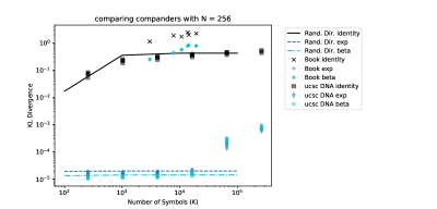
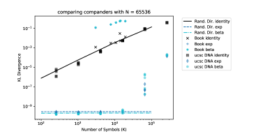
Figure 5: Comparing the beta compander and the EDI method. The random data is drawn with ${\mathrm{Dir}}_{K}(1)$ (i.e. uniform).

The beta compander is not the easiest algorithm to implement however. It is necessary to compute an incomplete beta function in order to find the compander function $f$, which is not known to have a closed form expression. We reiterate Remark 4 that it is indeed interesting that the minimax compander, on the other hand, does have a closed form.

C-B Analysis of the Power Compander

Figure 6: Comparing theoretical performance (357) of the power compander to experimental results.

Starting with Theorem 2, we can use the asymptotic analysis to understand why the power compander works well for all distributions. The following proposition proves the first set of results in Theorem 5.

Proposition 13.

Let single-letter density $p$ be the marginal probability of one letter on any symmetric probability distribution $P$ over $K$ letters. For the power compander $f(x)=x^{s}$ where $s\leq\frac{1}{2}$,

$$\widetilde{L}(p,f)\leq\frac{1}{K}\frac{1}{24}s^{-2}K^{2s}$$ (355)

and for any prior $P\in{\mathcal{P}}^{\triangle}_{K}$,

$$\widetilde{{\mathcal{L}}}_{K}(P,x^{s})\leq\frac{1}{24}s^{-2}K^{2s}\,.$$ (356)

Optimizing over $s$ gives

$$\widetilde{{\mathcal{L}}}_{K}(P,f)\leq\frac{e^{2}}{24}\log^{2}K\,.$$ (357)

Proof.

Since $f(x)=x^{s}$ we have that $f^{\prime}(x)=sx^{s-1}$. Using Theorem 2, this gives

$$\widetilde{L}(p,f)$$

$$=\frac{1}{24}s^{-2}\int_{0}^{1}x^{1-2s}p(x)dx=\frac{1}{24}s^{-2}{\mathbb{E}}_{X\sim p}[X^{1-2s}]\,.$$ (358)

The function $x^{1-2s}$ is increasing and also a concave function. We want to find the maximin prior distribution $P\in{\mathcal{P}}^{\triangle}_{K}$ (with marginals $p$) with the constraint

$$\sum_{i}{\mathbb{E}}_{X_{i}\sim p}[X_{i}] =1$$ (359)

(another constraint is that values of $p$ are such that must sum to one, but we give a weaker constraint here).

We want to choose $P$ to maximize

$$\sum_{i}{\mathbb{E}}_{X_{i}\sim p}[X_{i}^{1-2s}] ={\mathbb{E}}_{(X_{1},...,X_{K})\sim P}\left[\sum_{i}X_{i}^{1-2s}\right]\,.$$ (360)

By concavity (even ignoring any constraint that $P$ is symmetric), the maximum solution is given when $X_{1}=\dots=X_{K}$. Therefore, the maximin $P$ is such that the marginal on one letter $p$ is

$$p(1/K)=1\,.$$ (361)

The probability mass function where $1/K$ occurs with probability $1$ is a limit point of a sequence of continuous densities of the form

$$p(x)=\frac{1}{2\varepsilon}\text{ on }x\in\left[\frac{1}{K}-\varepsilon,\frac{1}{K}+\varepsilon\right]$$ (362)

as $\varepsilon\to 0$. We use this since we are restricting to continuous probability distributions.

Evaluating with this gives

$$\widetilde{L}(p,f) =\frac{1}{24}s^{-2}{\mathbb{E}}_{X\sim p}[X^{1-2s}]$$ (363)

$$\leq\frac{1}{24}s^{-2}\left(\frac{1}{K}\right)^{1-2s}$$ (364)

$$=\frac{1}{K}\frac{1}{24}s^{-2}K^{2s}$$ (365)

which shows (357). Multiplying by $K$ gives $\widetilde{\mathcal{L}}_{K}(P,f)$ for symmetric $P$.

Note that for any non-symmetric $P$, we can always symmetrize $P$ to a symmetric prior $P_{sym}$ by averaging over all random permutations of the indices. Because the loss $\widetilde{\mathcal{L}}_{K}(P,f)$ is concave in $P$, the symmetrized prior $P_{sym}$ will give an higher value, that is $\widetilde{\mathcal{L}}_{K}(P,f)\leq\widetilde{\mathcal{L}}_{K}(P_{sym},f)$. Hence $\widetilde{\mathcal{L}}_{K}(P,f)\leq\frac{1}{24}s^{-2}K^{2s}$ holds for all priors.

Finding the $s$ which minimizes $\frac{1}{24}s^{-2}K^{2s}$ is equivalent to finding $s$ which minimizes $s\log K-\log s$.

$$0 =\frac{d}{ds}s\log K-\log s=\log K-\frac{1}{s}$$ (366)

$$\implies s=\frac{1}{\log K}\,.$$ (367)

We can plug this back into our equation, using the fact that $e^{\log K}=K$ implies that $K^{\frac{1}{\log K}}=e$.

Thus, using $f(x)=x^{\frac{1}{\log K}}$ gives that

$$\widetilde{{\mathcal{L}}}_{K}(P,f)\leq\frac{e^{2}}{24}\log^{2}K\text{ for any }P\in{\mathcal{P}}^{\triangle}_{K}\,.$$ (368)

To generate a prior $P\in{\mathcal{P}}^{\triangle}_{K}$ that matches this upper bound, we note that this means we want its marginal $p$ to maximize $\frac{1}{24}(\log^{2}K){\mathbb{E}}_{X\sim p}[X^{1-2/\log K}]$, and from before we know that fixing $X=1/K$ does this (since ${\mathbb{E}}_{X\sim p}[X]=1/K$ as $p$ is the marginal of $P$). While $p$ has to represent a probability density function, and therefore cannot be a point mass, we can restrict its support to an arbitrarily small neighborhood around $1/K$ (and it is obvious that there are priors $P\in{\mathcal{P}}^{\triangle}_{K}$ with such a marginal), thus getting a match and showing that

$$\underset{P\in{\mathcal{P}}^{\triangle}_{K}}{\sup}\widetilde{{\mathcal{L}}}_{K}(P,f)=\frac{e^{2}}{24}\log^{2}K\,.$$ (369)

∎

The power compander turns out to give guarantees bounds on the value on $\widetilde{{\mathcal{L}}}_{K}(P,f)$ when $f$ is chosen so that $s={1}/{\log K}$. We show the comparison between this theoretical result on raw loss with the experimental results in Figure 6.

C-C Converging to Theoretical

For both the power compander and the beta compander, we show in Figure 7 how quickly the experimental results converge to the theoretical results. Experimental results have a fixed granularity $N$ whereas the theoretical results assume that $N\to\infty$. The plots show that by $N=2^{16}$ (each value gets $16$ bits), the experimental results for the power compander are very close to the theoretical results, and even for $N=2^{8}$ they are not so far. For the beta compander, the experimental results are close to the theoretical when $K$ is large. When $K=100$, the results for $N=2^{16}$ is not that close to the theoretical result, which demonstrates the effect of using unnormalized (or raw) values. The difference between normalizing and not normalizing gets smaller as $K$ increases.

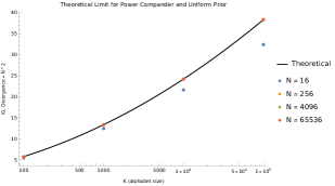
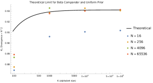
Figure 7: Comparing theoretical expression $\widetilde{L}(p,f)$ with experimental result. The KL divergence value of the experimental results are multiplied to $N^{2}$ in order to be comparable to $\widetilde{L}(p,f)$.

Appendix D Minimax and Approximate Minimax Companders

In this appendix, we analyze the minimax compander and approximate minimax compander. Specifically, we analyze the constant $c_{K}$, to show that it falls in $[1/4,3/4]$ (Section D-A) and that $\lim_{K\to\infty}c_{K}=1/2$ (Section D-A2). We also show that when $c_{K}$ is close to $1/2$, the approximate minimax compander (which is the same as the minimax compander except it replaces $c_{K}$ with $1/2$) has performance close to the minimax compander against all priors $p\in{\mathcal{P}}$ (Section D-B).

D-A Analysis of Minimax Companding Constant

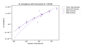
Figure 8: Comparing theoretical performance (110) of the approximate minimax compander to experimental results.

D-A1 Determining bounds on $c_{K}$

If $a_{K},b_{K}\geq 0$, then $p(x)$ is well-behaved (and bigger than $0$).

We need $a_{K}$ and $b_{K}$ to be such that $p(x)$ is a density that integrates to $1$ and also that $p(x)$ has expected value of $1/K$. To do this, first we compute that

$${\mathbb{E}}_{X\sim p}[X] =\int_{0}^{1}x\left(a_{K}x^{1/3}+b_{K}x^{4/3}\right)^{-3/2}\,dx$$ (370)

$$=\frac{-2}{b_{K}\sqrt{a_{K}+b_{K}}}+\frac{2\mathrm{ArcSinh}\left(\sqrt{\frac{b_{K}}{a_{K}}}\right)}{b_{K}^{3/2}}\,.$$ (371)

The constraint that $\int_{0}^{1}p(x)\,dx=1$ requires that $a_{K}\sqrt{a_{K}+b_{K}}=2$. We can use this to get

$${\mathbb{E}}_{X\sim p}[X] =\frac{-a_{K}}{b_{K}}+\frac{a_{K}\sqrt{\frac{a_{K}}{b_{K}}+1}\mathrm{ArcSinh}\left(\sqrt{\frac{b_{K}}{a_{K}}}\right)}{b_{K}}$$ (372)

$$=\frac{-1}{r}+\frac{\sqrt{\frac{1}{r}+1}\mathrm{ArcSinh}\left(\sqrt{r}\right)}{r}$$ (373)

$$=\frac{-1}{r}+\frac{\sqrt{\frac{1}{r}+1}\log\left(\sqrt{r}+\sqrt{r+1}\right)}{r}$$ (374)

where we use $r=b_{K}/a_{K}$. We will find upper and lower bounds in order to approximate what $r$ should be. Using (374), we can get

$${\mathbb{E}}_{X\sim p}[X] \leq\frac{1}{2}\frac{\log r}{r}$$ (375)

so long as $r>3$. If we choose $r=c_{1}K\log K$ and set $c_{1}=.75$, then

$${\mathbb{E}}_{X\sim p}[X] \leq\frac{1}{2}\frac{\log(c_{1}K\log K)}{c_{1}K\log K}$$ (376)

$$\leq\frac{1}{2c_{1}K}+\frac{\log\log K}{2c_{1}K\log K}+\frac{\log c_{1}}{2c_{1}K\log K}\leq\frac{1}{K}$$ (377)

so long as $K>4$. Similarly, we have

$${\mathbb{E}}_{X\sim p}[X] \geq\frac{1}{3}\frac{\log r}{r}$$ (378)

for all $r$. If we choose $r=c_{2}K\log K$ and set $c_{2}=.25$, then

$${\mathbb{E}}_{X\sim p}[X] \geq\frac{1}{3}\frac{\log(c_{2}K\log K)}{c_{2}K\log K}\geq\frac{1}{K}$$ (379)

so long as $K>24$.

Changing the value of $c$ changes the value of ${\mathbb{E}}_{X\sim p}[X]$ continuously. Hence, for each $K>24$, there exists a $c_{K}$ so that if $r=c_{K}K\log K$, then

$${\mathbb{E}}_{X\sim p}[X]=\frac{1}{K}\,.$$ (380)

such that $.25<c_{K}<.75$.

This proves the result for $K>24$; numerical evaluation of $c_{K}$ for $K=5,6,\dots,24$ then confirms that the result holds for all $K>4$.

D-A2 Limiting value of $c_{K}$

Lemma 11.

In the limit, $c_{K}\to 1/2$.

Proof.

We start with $r=\frac{b_{K}}{a_{K}}=c_{K}K\log K$, and we need to meet the condition that

$$\frac{-1}{r}+\frac{\sqrt{\frac{1}{r}+1}\log\left(\sqrt{r}+\sqrt{r+1}\right)}{r}=\frac{1}{K}\,.$$ (381)

Substituting we get

$$\frac{1}{K} =\frac{-1}{c_{K}K\log K}+\sqrt{\frac{1}{c_{K}K\log K}+1}$$

$$\quad\quad\frac{\log\left(\sqrt{c_{K}K\log K}+\sqrt{c_{K}K\log K+1}\right)}{c_{K}K\log K}$$ (382)

$$\implies c_{K}=\frac{-1}{\log K}+\sqrt{\frac{1}{c_{K}K\log K}+1}$$

$$\quad\quad\frac{\log\left(\sqrt{c_{K}K\log K}+\sqrt{c_{K}K\log K+1}\right)}{\log K}\,.$$ (383)

Let $c=\lim_{K\to\infty}c_{K}$. Since $c_{K}$ is bounded, we know that $\lim_{K\to\infty}c_{K}K\log K=\infty$ since $c_{K}$ is bounded below by $1/4$; additionally $\log c_{K}$ is bounded (above and below) since for $K>4$ we have $c_{K}\in[1/4,3/4]$.

$$c =\lim_{K\to\infty}\frac{-1}{\log K}$$

$$\quad\quad+\sqrt{\frac{1}{c_{K}K\log K}+1}$$

$$\quad\quad\frac{\log\left(\sqrt{c_{K}K\log K}+\sqrt{c_{K}K\log K+1}\right)}{\log K}$$ (384)

$$=0+1\lim_{K\to\infty}\frac{\log\left(2\sqrt{c_{K}K\log K}\right)}{\log K}$$ (385)

$$=\lim_{K\to\infty}\frac{\log 2+\frac{1}{2}\log c_{K}+\frac{1}{2}\log K+\frac{1}{2}\log\log K}{\log K}$$ (386)

$$=\frac{1}{2}\,.$$ (387)

∎

D-B Approximate Minimax Compander vs. Minimax Compander

For any $K$, $c_{K}$ can be approximated numerically. To simplify the quantizer, recall we can use $c_{K}\approx\frac{1}{2}$ for large $K$ to get the approximate minimax compander (21).

This is close to optimal without needing to compute $c_{K}$. Here we prove Proposition 4.

Proof.

Since $f^{*}_{K},f^{**}_{K}\in{\mathcal{F}}^{\dagger}$, we know that

$$\widetilde{L}(p,f^{*}_{K})=L^{\dagger}(p,f^{*}_{K})\leavevmode\nobreak\ \text{ and }\leavevmode\nobreak\ \widetilde{L}(p,f^{**}_{K})=L^{\dagger}(p,f^{**}_{K})\,.$$ (388)

We define the corresponding asymptotic local loss functions

$$g^{*}(x) =\frac{1}{24}(f^{*}_{K})^{\prime}(x)^{-2}x^{-1}$$ (389)

$$g^{**}(x) =\frac{1}{24}(f^{**}_{K})^{\prime}(x)^{-2}x^{-1}$$ (390)

so that our goal is to prove

$$\int g^{**}\,dp\leq(1+\varepsilon)\int g^{*}\,dp\,.$$ (391)

Let $\gamma^{*}=c_{K}(K\log K)$ and $\gamma^{**}=\frac{1}{2}(K\log K)$ (the constants in $f^{*}_{K}$ and $f^{**}_{K}$ respectively) and let $\phi^{*}(x)=\mathrm{ArcSinh}(\sqrt{\gamma^{*}x})$ and $\phi^{**}(x)=\mathrm{ArcSinh}(\sqrt{\gamma^{**}x})$. Then

$$(\phi^{*})^{\prime}(x) =\frac{\sqrt{\gamma^{*}}}{2\sqrt{x}\sqrt{\gamma^{*}x+1}}$$ (392)

$$\text{and }\leavevmode\nobreak\ (\phi^{**})^{\prime}(x) =\frac{\sqrt{\gamma^{**}}}{2\sqrt{x}\sqrt{\gamma^{**}x+1}}\,.$$ (393)

Note that $f^{*}_{K}(x)=\phi^{*}(x)/\phi^{*}(1)$ and $f^{**}_{K}(x)=\phi^{**}(x)/\phi^{**}(1)$. We now split into two cases: (i) $c_{K}>1/2$ and (ii) $c_{K}<1/2$.

In case (i) (which implies $\gamma^{*}>\gamma^{**}$, and note that $\gamma^{*}/\gamma^{**}=2c_{K}\leq 1+\varepsilon$), we get for all $x\in[0,1]$,

$$\frac{(\phi^{*})^{\prime}(x)}{(\phi^{**})^{\prime}(x)} =\sqrt{\frac{\gamma^{*}}{\gamma^{**}}}\sqrt{\frac{\gamma^{**}x+1}{\gamma^{*}x+1}}$$ (394)

$$\quad\quad\in[1,\sqrt{\gamma^{*}/\gamma^{**}}]\ \subseteq[1,\sqrt{1+\varepsilon}]$$ (395)

since $\sqrt{\frac{\gamma^{**}x+1}{\gamma^{*}x+1}}\in[\sqrt{\gamma^{**}/\gamma^{*}},1]$. Because $\gamma^{*}\geq\gamma^{**}$ and $\mathrm{ArcSinh}$ is an increasing function, we know that $\phi^{*}(1)\geq\phi^{**}(1)$. Thus, for any $x\in[0,1]$,

$$(f^{**}_{K})^{\prime}(x) =\frac{(\phi^{**})^{\prime}(x)}{\phi^{**}(1)}$$ (396)

$$\geq\frac{\frac{1}{\sqrt{1+\varepsilon}}(\phi^{*})^{\prime}(x)}{\phi^{*}(1)}$$ (397)

$$=\frac{1}{\sqrt{1+\varepsilon}}(f^{*}_{K})^{\prime}(x)$$ (398)

$$\implies(f^{**}_{K})^{\prime}(x)^{-2} \leq(1+\varepsilon)(f^{*}_{K})^{\prime}(x)^{-2}$$ (399)

$$\implies g^{**}(x) \leq(1+\varepsilon)g^{*}(x)$$ (400)

$$\implies\int g^{**}\,dp \leq(1+\varepsilon)\int g^{*}\,dp$$ (401)

which is what we wanted to prove.

Case (ii), where $c_{K}<1/2$ (implying $\gamma^{**}>\gamma^{*}$) can be proved analogously:

$$\frac{(\phi^{**})^{\prime}(x)}{(\phi^{*})^{\prime}(x)} =\sqrt{\frac{\gamma^{**}}{\gamma^{*}}}\sqrt{\frac{\gamma^{*}x+1}{\gamma^{**}x+1}}$$ (402)

$$\quad\quad\in[1,\sqrt{\gamma^{**}/\gamma^{*}}]\subseteq[1,\sqrt{1+\varepsilon}]$$ (403)

which then gives us $(\phi^{**})^{\prime}(x)\geq(\phi^{*})^{\prime}(x)$ and

$$\phi^{**}(1) =\int_{0}^{1}(\phi^{**})^{\prime}(t)\,dt$$ (404)

$$\leq\sqrt{1+\varepsilon}\int_{0}^{1}(\phi^{*})^{\prime}(t)\,dt$$ (405)

$$\leq(\sqrt{1+\varepsilon})\phi^{*}(1)\,.$$ (406)

Thus, for any $x\in[0,1]$,

$$(f^{**}_{K})^{\prime}(x) =\frac{(\phi^{**})^{\prime}(x)}{\phi^{**}(1)}$$ (407)

$$\geq\frac{(\phi^{*})^{\prime}(x)}{(\sqrt{1+\varepsilon})\phi^{*}(1)}$$ (408)

$$=\frac{1}{\sqrt{1+\varepsilon}}(f^{*}_{K})^{\prime}(x)$$ (409)

$$\implies(f^{**}_{K})^{\prime}(x)^{-2} \leq(1+\varepsilon)(f^{*}_{K})^{\prime}(x)^{-2}$$ (410)

$$\implies g^{**}(x) \leq(1+\varepsilon)g^{*}(x)$$ (411)

$$\implies\int g^{**}\,dp \leq(1+\varepsilon)\int g^{*}\,dp$$ (412)

completing the proof for both cases. ∎

We show the comparison of the theoretical (asymptotic in $K$ result) of the approximate minimax compander with the experimental results in Figure 8.

Appendix E Worst-Case Analysis

In this section, we prove Theorem 4 which applies both to the minimax compander and the power compander. Since we are dealing with worst-case (i.e. not a random ${\boldsymbol{x}}$) the centroid is not defined; therefore this theorem works with the midpoint decoder. Thus, the (raw) decoded value of $x$ is $\bar{y}_{(n_{N}(x))}$.

Additionally, we are not using the raw reconstruction but the normalized reconstruction, and hence it does not suffice to deal with a single letter at a time. Thus, we will work with a full probability vector ${\boldsymbol{x}}\in\triangle_{K-1}$.

Proof of Theorem 4 and (47) in Theorem 5.

Let ${\boldsymbol{x}}\in\triangle_{K-1}$ be the vector we are quantizing, with $i$th element (out of $K$, summing to $1$) $x_{i}$; since we are dealing with midpoint decoding, our (raw) decoded value of $x_{i}$ is $\bar{y}_{n_{N}(x_{i})}$. For simplicity, let us denote it as $\bar{y}_{i}$, and the normalized value as $z_{i}=\bar{y}_{i}/\big{(}\sum_{j}\bar{y}_{j}\big{)}$.

Let $\delta_{i}=\bar{y}_{i}-x_{i}$ be the difference between the raw decoded value $\bar{y}_{i}$ and the original value $x_{i}$. Then:

$$D_{\operatorname{{\scriptscriptstyle KL}}} \left({\boldsymbol{x}}\|\boldsymbol{z}\right)=\sum_{i}x_{i}\log\frac{x_{i}}{z_{i}}$$ (413)

$$=\sum_{i}x_{i}\log\frac{x_{i}}{\bar{y}_{i}}+\log\Big{(}\sum_{i}\bar{y}_{i}\Big{)}$$ (414)

$$=\sum_{i}(\bar{y}_{i}-\delta_{i})\log\frac{\bar{y}_{i}-\delta_{i}}{\bar{y}_{i}}+\log\Big{(}1+\sum_{i}\delta_{i}\Big{)}\,.$$ (415)

Next we use that $\log(1+w)\leq w$.

$$D_{\operatorname{{\scriptscriptstyle KL}}}\left({\boldsymbol{x}}\|\boldsymbol{z}\right) \leq\sum_{i}(\bar{y}_{i}-\delta_{i})\frac{-\delta_{i}}{\bar{y}_{i}}+\sum_{i}\delta_{i}$$ (416)

$$=\sum_{i}-\delta_{i}+\sum_{i}\frac{\delta_{i}^{2}}{\bar{y}_{i}}+\sum_{i}\delta_{i}$$ (417)

$$=\sum_{i}\frac{(\bar{y}_{i}-x_{i})^{2}}{\bar{y}_{i}}$$ (418)

(note that in (416) we used the inequality $\log(1+w)\leq w$ on both appearances of the logarithm, as well as the fact that $\bar{y}_{i}-\delta_{i}=x_{i}\geq 0$).

We now consider each bin $I^{(n)}$ induced by $f$. For simplicity let the dividing points between the bins be denoted by

$$\beta_{(n)}=f^{-1}\Big{(}\frac{n}{N}\Big{)}=\bar{y}_{(n)}+r_{(n)}/2$$ (419)

(where $r_{(n)}$ is the width of the $n$th bin) so that $I^{(n)}=(\beta_{(n-1)},\beta_{(n)}]$. Since all the companders we are discussing are strictly monotonic, there is no ambiguity. Then, the Mean Value Theorem (which we can use since the minimax compander, the approximate minimax compander, and the power compander are all continuous and differentiable ) says that, for each $I^{(n)}$ there is some value $w_{(n)}$ such that

$$f^{\prime}(w_{(n)})=\frac{f(\beta_{(n)})-f(\beta_{(n-1)})}{\beta_{(n)}-\beta_{(n-1)}}=N^{-1}r_{(n)}^{-1}$$ (420)

(since $f(\beta_{(n)})-f(\beta_{(n-1)})=n/N-(n-1)/N=1/N$ and $\beta_{(n)}-\beta_{(n-1)}=r_{(n)}$ by definition).

Thus, we can re-write this as follows:

$$r_{(n)}=N^{-1}f^{\prime}(w_{(n)})^{-1}\,.$$ (421)

We will also denote the following for simplicity: $I_{i}=I^{(n_{N}(x_{i}))}$; $r_{i}=r_{(n_{N}(x_{i}))}$; and $w_{i}=w_{(n_{N}(x_{i}))}$ (the bin, bin length, and bin mean value corresponding to $x_{i}$).

Trivially, since $w_{i}\in I_{i}$, we know that $\frac{w_{i}}{2}\leq\bar{y}_{i}$. Thus, we can derive (since $\bar{y}_{i}$ is the midpoint of $I_{i}$ and $x_{i}\in I_{i}$, we know that $|\bar{y}_{i}-x_{i}|\leq r_{i}/2$) that

$$D_{\operatorname{{\scriptscriptstyle KL}}}\left({\boldsymbol{x}}\|\boldsymbol{z}\right) \leq\sum_{i}\frac{(\bar{y}_{i}-x_{i})^{2}}{\bar{y}_{i}}$$ (422)

$$\leq\frac{1}{4}\sum_{i}\frac{r_{i}^{2}}{\bar{y}_{i}}$$ (423)

$$\leq\frac{1}{4}\sum_{i}\frac{1}{N^{2}(w_{i}/2)(f^{\prime}(w_{i}))^{2}}$$ (424)

$$=\frac{1}{2}N^{-2}\sum_{i}\frac{1}{w_{i}(f^{\prime}(w_{i}))^{2}}\,.$$ (425)

Note that while we are using midpoint decoding for our quantization, for the purposes of analysis, it is more convenient to express the all the terms in the KL divergence loss using the mean value.

We now examine the worst case performance of the three companders: the power compander, the minimax compander, and the approximate minimax compander.

Power compander: In this case, we have

$$f(x)=x^{s}\text{ and }f^{\prime}(x)=sx^{s-1}$$ (426)

for $s=\frac{1}{\log K}$ (which is optimal for minimizing raw distortion against worst-case priors). This yields

$$D_{\operatorname{{\scriptscriptstyle KL}}}\left({\boldsymbol{x}}\|\boldsymbol{z}\right) \leq\frac{1}{2}N^{-2}s^{-2}\sum_{i}\frac{1}{w_{i}w_{i}^{2s-2}}$$ (427)

$$=\frac{1}{2}N^{-2}s^{-2}\sum_{i}w_{i}^{1-2s}\,.$$ (428)

So long as $s<1/2$ (which occurs for $K>7$), the function $w_{i}^{1-2s}$ is concave in $w_{i}$. Thus, replacing all $w_{i}$ by their average will increase the value. Furthermore, $K^{s}=K^{\frac{1}{\log K}}=e$. Thus, we can derive:

$$D_{\operatorname{{\scriptscriptstyle KL}}}\left({\boldsymbol{x}}\|\boldsymbol{z}\right) \leq\frac{1}{2}N^{-2}s^{-2}K\left(\frac{\sum_{i}w_{i}}{K}\right)^{1-2s}$$ (429)

$$=\frac{1}{2}N^{-2}(\log^{2}K)e^{2}\Big{(}\sum_{i}w_{i}\Big{)}^{1-2s}$$ (430)

$$\leq\frac{e^{2}}{2}N^{-2}(\log^{2}K)\max\Big{\{}1,\sum_{i}w_{i}\Big{\}}\,.$$ (431)

Next, we need to bound $\max\left\{1,\sum_{i}w_{i}\right\}$. Assume that $\sum_{i}w_{i}>1$ (otherwise our bound is just $1$). Then, we note the following: $\sum_{i}x_{i}=1$ by definition; $s^{-1}=\log K$; and

$$r_{i}=N^{-1}f^{\prime}(w_{i})^{-1}=N^{-1}s^{-1}w_{i}^{1-s}\,.$$ (432)

This allows us to make the following derivation:

$$\sum_{i}|w_{i}-x_{i}| \leq\frac{1}{2}\sum_{i}r_{i}$$ (433)

$$\implies\sum_{i}w_{i} \leq\sum_{i}x_{i}+\frac{1}{2}N^{-1}s^{-1}\sum_{i}w_{i}^{1-s}$$ (434)

$$\leq 1+\frac{1}{2}N^{-1}\log(K)K\left(\frac{\sum_{i}w_{i}}{K}\right)^{1-s}$$ (435)

$$=1+\frac{e}{2}N^{-1}\log(K)\Big{(}\sum_{i}w_{i}\Big{)}^{1-s}$$ (436)

$$\leq 1+\frac{e}{2}N^{-1}\log(K)\Big{(}\sum_{i}w_{i}\Big{)}\,.$$ (437)

We get (435) by the same concavity trick: because $w_{i}^{1-s}$ is concave in $w_{i}$, replacing each individual $w_{i}$ with their average can only increase the sum. We get (436) because $K^{s}=K^{\frac{1}{\log K}}=e$.

We can combine terms with $\sum_{i}w_{i}$.

$$\left(1-\frac{e}{2}N^{-1}\log K\right)\sum_{i}w_{i}\leq 1\,.$$ (438)

This implies that if $N>\frac{e}{2}\log K$, then

$$\sum_{i}w_{i} \leq\frac{1}{1-\frac{e}{2}N^{-1}\log K}$$ (439)

$$=\frac{N}{N-\frac{e}{2}\log K}=1+\frac{e}{2}\frac{\log K}{N-\frac{e}{2}\log K}\,.$$ (440)

Furthermore, if $N\geq e\log K$, we get that $\sum_{i}w_{i}\leq 2$. Combining (431) with (440), we have

$$D_{\operatorname{{\scriptscriptstyle KL}}}({\boldsymbol{x}}\|\boldsymbol{z})$$

$$\leq\frac{e^{2}}{2}N^{-2}(\log^{2}K)\max\left\{1,\left(1+\frac{e}{2}\frac{\log K}{N-\frac{e}{2}\log K}\right)\right\}$$ (441)

$$=\frac{e^{2}}{2}N^{-2}(\log^{2}K)\left(1+\frac{e}{2}\frac{\log K}{N-\frac{e}{2}\log K}\right)$$ (442)

for $N>\frac{e}{2}\log K$. When $N\geq e\log K$, this becomes the pleasing

$$D_{\operatorname{{\scriptscriptstyle KL}}}({\boldsymbol{x}}\|\boldsymbol{z})\leq e^{2}N^{-2}\log^{2}K\,.$$ (443)

Minimax compander and approximate minimax compander: Since they are very similar in form, it is convenient to do both at once. Let $c$ be a constant which is either $c_{K}$ if we are considering the minimax compander, or $\frac{1}{2}$ if we’re considering the approximate minimax compander; and let $\gamma=cK\log K$. Then our compander and its derivative will have the form

$$f(x) =\frac{\mathrm{ArcSinh}(\sqrt{\gamma x})}{\mathrm{ArcSinh}(\sqrt{\gamma})}$$ (444)

$$f^{\prime}(x) =\frac{1}{2\mathrm{ArcSinh}(\sqrt{\gamma})}\frac{\sqrt{\gamma}}{\sqrt{x}\sqrt{1-\gamma x}}$$ (445)

$$\implies f^{\prime}(x)^{-1} =2\mathrm{ArcSinh}(\sqrt{\gamma})\sqrt{\frac{x}{\gamma}+x^{2}}\,.$$ (446)

This then yields that

$$r_{i} =N^{-1}f^{\prime}(w_{i})^{-1}$$ (447)

$$=2N^{-1}\mathrm{ArcSinh}(\sqrt{\gamma})\sqrt{\frac{w_{i}}{\gamma}+w_{i}^{2}}\,.$$ (448)

Then we can derive from (425) that

$$D_{\operatorname{{\scriptscriptstyle KL}}}({\boldsymbol{x}}\|\boldsymbol{z})\leq\frac{1}{2}N^{-2}(2\mathrm{ArcSinh}(\sqrt{\gamma}))^{2}\sum_{i}\frac{\frac{w_{i}}{\gamma}+w_{i}^{2}}{w_{i}}$$ (449)

$$=2N^{-2}(\mathrm{ArcSinh}(\sqrt{\gamma}))^{2}\left(\frac{K}{\gamma}+\sum_{i}w_{i}\right)$$ (450)

$$\leq 2N^{-2}(\mathrm{ArcSinh}(\sqrt{\gamma}))^{2}\left(\frac{K}{\gamma}+\max\left\{1,\sum_{i}w_{i}\right\}\right)\,.$$ (451)

Assuming that $\sum_{i}w_{i}>1$ (otherwise the bound is just $1$),

$$\sum_{i}|w_{i}-x_{i}| \leq\sum_{i}\frac{r_{i}}{2}$$ (452)

$$\implies\sum_{i}w_{i} \leq\sum_{i}x_{i}+N^{-1}\mathrm{ArcSinh}(\sqrt{\gamma})\sum_{i}\sqrt{\frac{w_{i}}{\gamma}+w_{i}^{2}}$$ (453)

$$=1+N^{-1}\mathrm{ArcSinh}(\sqrt{\gamma})\sum_{i}\sqrt{\frac{w_{i}}{\gamma}+w_{i}^{2}}\,.$$ (454)

To bound the sum in (454), using the fact that $\sqrt{\cdot}$ is concave (so averaging the inputs of a sum of square roots makes it bigger), we get

$$\sum_{i}\sqrt{\frac{w_{i}}{\gamma}+w_{i}^{2}} \leq\sum_{i}\sqrt{\frac{w_{i}}{\gamma}}+\sqrt{w_{i}^{2}}$$ (455)

$$\leq K\left(\frac{\sum_{i}w_{i}}{K(cK\log K)}\right)^{1/2}+\sum_{i}w_{i}$$ (456)

$$\leq\left(\frac{\sum_{i}w_{i}}{c\log K}\right)^{1/2}+\sum_{i}w_{i}$$ (457)

$$\leq\frac{\sum_{i}w_{i}}{(c\log K)^{1/2}}+\sum_{i}w_{i}$$ (458)

$$=\Big{(}\sum_{i}w_{i}\Big{)}\left(1+\frac{1}{(c\log K)^{1/2}}\right)$$ (459)

$$=\eta\Big{(}\sum_{i}w_{i}\Big{)}$$ (460)

where $\eta=1+(c\log K)^{-1/2}$. Then (454) becomes

$$\sum_{i}w_{i} \leq 1+\eta N^{-1}\mathrm{ArcSinh}(\sqrt{\gamma})\Big{(}\sum_{i}w_{i}\Big{)}\,.$$ (461)

Since we have $\sum_{i}w_{i}$ on both sides of the equation, we can combine these terms like before.

$$(1-\eta N^{-1}\mathrm{ArcSinh}(\sqrt{\gamma}))\sum_{i}w_{i}\leq 1$$ (462)

$$\implies \sum_{i}w_{i}\leq\frac{N}{N-\eta\mathrm{ArcSinh}(\sqrt{\gamma})}$$ (463)

if $N>\eta\mathrm{ArcSinh}(\sqrt{\gamma})$. Combining these and using the expression $\mathrm{ArcSinh}(\sqrt{w})=\log(\sqrt{w+1}+\sqrt{w})\leq\log(2\sqrt{w}+1)$ we get from (451) that

$$D_{\operatorname{{\scriptscriptstyle KL}}}({\boldsymbol{x}}\|\boldsymbol{z})$$

$$\leq 2N^{-2}(\mathrm{ArcSinh}(\sqrt{\gamma}))^{2}$$

$$\quad\quad\left(\frac{K}{\gamma}+\frac{N}{N-\eta\mathrm{ArcSinh}(\sqrt{\gamma})}\right)$$ (464)

$$=2N^{-2}(\mathrm{ArcSinh}(\sqrt{cK\log K}))^{2}$$

$$\quad\quad\left(\frac{K}{cK\log K}+\frac{N}{N-\eta\mathrm{ArcSinh}(\sqrt{cK\log K})}\right)$$ (465)

$$\leq 2N^{-2}(\log(2\sqrt{cK\log K}+1))^{2}$$

$$\quad\quad\left(\frac{1}{c\log K}+\frac{N}{N-\eta\log(2\sqrt{cK\log K}+1)}\right)\,.$$ (466)

This holds for all $N>\eta\log(2\sqrt{cK\log K}+1)$; furthermore, if $N>3\eta\log(2\sqrt{cK\log K}+1)$, the second term in the parentheses is at most $3/2$ (and if $N$ is larger, this term goes to $1$). Recall $c$ is between $1/4$ and $3/4$ (as it is either $c_{K}$ or $1/2$) when $K>4$. Then, we know that for all $K>4$ that $\eta<2.57\dots$ and $1/(c\log K)<5/2$. Thus, for

$$N >8\log(2\sqrt{cK\log K}+1)$$ (467)

$$>3(2.6)\log(2\sqrt{cK\log K}+1)$$ (468)

$$>3\eta\log(2\sqrt{cK\log K}+1)$$ (469)

we can bound the entire parenthesis term by $4$. Then,

$$D_{\operatorname{{\scriptscriptstyle KL}}} ({\boldsymbol{x}}\|\boldsymbol{z})\leq 8N^{-2}(\log(2\sqrt{cK\log K}+1))^{2}$$ (470)

$$\leq 8N^{-2}(\log(3\sqrt{cK\log K}))^{2}$$ (471)

$$=2N^{-2}(\log(cK\log K)+2\log 3)^{2}$$ (472)

$$=2N^{-2}\Big{(}1+O\Big{(}\frac{\log\log K}{\log K}\Big{)}\Big{)}\log^{2}K\,.$$ (473)

Note that whether $c$ is $c_{K}$ or $1/2$, it is always between $1/4$ and $3/4$, and so it has no effect on the order of growth. We also note that the above (stated more crudely) is an order of growth within $O(N^{-2}\log^{2}K)$.

We can obtain a relatively clean upper bound on the error term $O\big{(}\frac{\log\log K}{\log K}\big{)}$ by setting $c=3/4$ (which is larger than the whole range of possible values); in this case, numerically computing (472), we get that the error term is at most $18\frac{\log\log K}{\log K}$ for $K>4$. The quantity $18\frac{\log\log K}{\log K}$ has a maximum value of around $6.62183$. ∎

The statement above (which is used for Theorem 4) computes constants for our bound which work for both the minimax compander and approximate minimax compander and only requires that $K>4$.

If we are only concerned with large alphabet sizes, to improve the constants for the approximate minimax compander (where $c=1/2$), we can instead use the following: For $K\geq 55$ and $N>6\log(2\sqrt{cK\log K}+1)$,

$$D_{\operatorname{{\scriptscriptstyle KL}}} ({\boldsymbol{x}}\|\boldsymbol{z})\leq N^{-2}\Big{(}1+6\frac{\log\log K}{\log K}\Big{)}\log^{2}K\,.$$ (474)

Appendix F Uniform Quantization

In this section, we examine of the performance of uniform quantization under KL divergence loss. This is the same as applying the truncate compander.

First, we will prove (28) of Remark 5.

Proof of (28).

Let $p$ be the single-letter distribution which is uniform over $\left[0,{2}/{K}\right]$ for each symbol. Specifically, the probability density function is

$$p(x)=\frac{K}{2}\text{ for }x\in\left[0,\frac{2}{K}\right]$$ (475)

and since the expected value under $p$ is $1/K$, we have that $p\in{\mathcal{P}}_{1/K}$.

We want to compute the single-letter loss for $p$, but notice that we cannot use Theorem 2 to do so, since the quantity $L^{\dagger}(p,f)$ is not finite here (this is not surprising since we are showing a case where the dependence of $\widetilde{L}(p,f,N)$ on $N$ is larger than $\Theta(N^{-2})$). Thus we need to compute the single-letter loss starting with (11).

$$\widetilde{L}(p,f,N) ={\mathbb{E}}_{X\sim p}\big{[}X\log(X/\widetilde{y}(X))\big{]}$$ (476)

$$=\sum_{n=1}^{N}\int_{I^{(n)}}p(x)x\log\frac{x}{\tilde{y}_{n}}dx$$ (477)

$$=\sum_{n=1}^{N}\int_{I^{(n)}}{\mathbb{I}}\{x<2/K\}\frac{K}{2}x\log\frac{x}{\tilde{y}_{n}}dx$$ (478)

$$\geq\frac{K}{2}\sum_{n=1}^{\lfloor 2N/K\rfloor}\int_{n/N}^{(n+1)/N}x\log\frac{x}{\tilde{y}_{n}}dx$$ (479)

$$=\frac{K}{2}\sum_{n=1}^{\lfloor 2N/K\rfloor}\int_{\tilde{y}_{n}-\frac{r}{2}}^{\tilde{y}_{n}+\frac{r}{2}}x\log\frac{x}{\tilde{y}_{n}}dx$$ (480)

where we let $r=1/N$.

Using the Taylor expansion for $\log(1+x)$, we can get that

$$\int_{\tilde{y}_{n}-\frac{r}{2}}^{\tilde{y}_{n}+\frac{r}{2}}x\log\frac{x}{\tilde{y}_{n}}dx=\frac{r^{3}}{24\tilde{y}_{n}}+O\left(\frac{r^{5}}{\tilde{y}_{n}^{3}}\right)\,.$$ (481)

This gives that

$$\widetilde{L}(p,f,N) \geq\frac{K}{2}\sum_{n=1}^{\lfloor 2N/K\rfloor}\frac{r^{3}}{24\tilde{y}_{n}}-O\left(\frac{r^{5}}{\tilde{y}_{n}^{3}}\right)$$ (482)

$$=\frac{K}{48}\frac{1}{N^{3}}\sum_{n=1}^{\lfloor 2N/K\rfloor}\frac{1}{\tilde{y}_{n}}-\sum_{n=1}^{\lfloor 2N/K\rfloor}O\left(\frac{1}{N^{5}\tilde{y}_{n}^{3}}\right)\,.$$ (483)

Because the intervals are uniform, the centroid is the midpoint of each interval, which means that

$$\tilde{y}_{n}=\frac{n-1/2}{N}\,.$$ (484)

This gives that

$$\sum_{n=1}^{\lfloor 2N/K\rfloor}\frac{1}{\tilde{y}_{n}} =\sum_{n=1}^{\lfloor 2N/K\rfloor}\frac{1}{\frac{n-1/2}{N}}$$ (485)

$$>N\sum_{n=1}^{\lfloor 2N/K\rfloor}\frac{1}{n}$$ (486)

$$>C_{1}N\log(2N/K)\,.$$ (487)

We also need to bound the smaller order terms to make sure they are not too big,

$$\sum_{n=1}^{\lfloor 2N/K\rfloor}\frac{1}{\tilde{y}_{n}^{3}} <N^{3}\left(2^{3}+\sum_{n=2}^{\lfloor 2N/K\rfloor}\frac{1}{(n-1)^{3}}\right)$$ (488)

$$=N^{3}C_{3}\,.$$ (489)

Combining these give

$$\widetilde{L}(p,f,N) \geq\frac{K}{48N^{3}}C_{1}N\log(2N/K)-O\left(\frac{1}{N^{2}}\right)$$ (490)

$$=\Omega\left(\frac{K}{N^{2}}\log N\right)\,.$$ (491)

All the inequalities we used for the lower bound can easily be adjusted to make an upper bound. For instance, the floor function in the summation can be replaced with a ceiling function. The quantity $\tilde{y}_{n}$ can be rounded up or down and the inequalities approximating sums can have different multiplicative constants. This gives that for $p(x)$, we have

$$\widetilde{L}(p,f,N)=\Theta\left(\frac{K}{N^{2}}\log N\right)\,.$$ (492)

Combining this single-letter density with the proof of Proposition 3 gives a prior $P$ over the simplex so that

$$\widetilde{{\mathcal{L}}}_{K}(P,f,N)=K\widetilde{L}(p,f,N)=\Theta\left(\frac{K^{2}}{N^{2}}\log N\right)\,.$$ (493)

when $f$ is the truncate compander.

We want to relate the raw loss in (493) to the expected loss ${\mathcal{L}}_{K}(P,f,N)$. This requires us to look at the normalization constant.

$${\mathbb{E}}_{{\boldsymbol{X}}\sim P} \left[\log\left(\sum_{k=1}^{K}\tilde{y}_{k}\right)\right]$$ (494)

$$={\mathbb{E}}_{{\boldsymbol{X}}\sim P}\left[\log\left(\sum_{k=1}^{K}\tilde{y}_{k}-\sum_{k=1}^{K}x_{k}+\sum_{k=1}^{K}x_{k}\right)\right]$$ (495)

$$={\mathbb{E}}_{{\boldsymbol{X}}\sim P}\left[\log\left(\sum_{k=1}^{K}\delta_{k}+1\right)\right]$$ (496)

where $\delta_{k}=\tilde{y}_{k}-x_{k}$. We can bound

$$-\frac{1}{2N}\leq\delta_{k}\leq\frac{1}{2N}$$ (497)

$$-\frac{K}{2N}\leq\sum_{k=1}^{K}\delta_{k}\leq\frac{K}{2N}\,.$$ (498)

Additionally, we know that by construction,

$${\mathbb{E}}_{{\boldsymbol{X}}\sim p}\left[\sum_{k=1}^{K}\delta_{k}\right]=\sum_{k=1}^{K}(\tilde{y}_{k}-x_{k})=0$$ (499)

since $\tilde{y}_{k}$ is produced by the centroid decoder. Therefore, since $\log$ is concave, we have

$${\mathbb{E}}_{{\boldsymbol{X}}\sim P} \left[\log\left(\sum_{k=1}^{K}\delta_{k}+1\right)\right]$$ (500)

$$\geq\frac{1}{2}\left(\log\left(1-\frac{K}{2N}\right)+\log\left(1+\frac{K}{2N}\right)\right)$$ (501)

$$\geq\frac{1}{2}\cdot 2\cdot\frac{-(K/(2N))^{2}}{2}$$ (502)

$$=-\frac{1}{8}K^{2}N^{-2}$$ (503)

where the second inequality follows from the Taylor series of $\log(1+w)$. But this means that

$$-{\mathbb{E}}_{{\boldsymbol{X}}\sim P}\left[\log\left(\sum_{k=1}^{K}\delta_{k}+1\right)\right]=O\left(\frac{K^{2}}{N^{2}}\right)$$ (504)

and hence by the proof of Proposition 1

$${\mathcal{L}}(P,f, N)$$ (505)

$$=\widetilde{{\mathcal{L}}}(P,f,N)+{\mathbb{E}}_{{\boldsymbol{X}}\sim P}\left[\log\left(\sum_{k=1}^{K}\delta_{k}+1\right)\right]$$ (506)

$$=\Theta\left(\frac{K^{2}}{N^{2}}\log N\right)+O\left(\frac{K^{2}}{N^{2}}\right)$$ (507)

$$=\Theta\left(\frac{K^{2}}{N^{2}}\log N\right)$$ (508)

since the extra $\log N$ factor causes the first term to dominate the second. ∎

The density $p(x)$ which produces (493) is not necessarily the worst possible density function in terms of the dependence of raw loss on the granularity $N$; however, it achieves simultaneously a worse-than-$\Theta(N^{-2})$ dependence on $N$ and a very large dependence on the alphabet size $K$ (namely $\Theta(K^{2})$) with the uniform quantizer (i.e. truncation), and is therefore an ideal example of why the uniform quantizer is vulnerable to having poor performance.

For illustration, we will also sketch an analysis of the performance of the uniform prior against prior $p(x)=(1-\alpha)x^{-\alpha}$ where $\alpha=\frac{K-2}{K-1}$ (as mentioned in Remark 5); this is constructed so that ${\mathbb{E}}_{X\sim p}[X]=1/K$ and hence $p\in{\mathcal{P}}_{1/K}$. The analysis shows that the loss is proportional to $N^{-(2-\alpha)}$.

Let $N$ be large; for this sketch we will treat $p$ as roughly uniform over any bin $I^{(n)}:=((n-1)/N,n/N]$. Note that this does not strictly hold for small $n$ (no matter how large $N$ gets, $p$ never becomes approximately uniform over e.g. $I^{(1)}$) but this inaccuracy is most pronounced on the first interval $I^{(1)}=(0,1/n]$. Additionally, $p$ on $(0,1/n]$ is a stretched and scaled version of $p$ on $(0,1]$; for $n=2,3,\dots,N$, the distribution $p$ over $I^{(n)}$ is closer to being uniform, and hence the distortion over any bin under $p$ can be bounded below (and above) by a constant multiple of the distortion under a uniform distribution (the constant can depend on $K$ but not $N$). Thus for determining the dependence of the (raw) distortion on $N$, this simplification does not affect the result.

Then, the expected distortion given that $X\in I^{(n)}$ is proportional (roughly) to $N^{-2}(n/N)^{-1}=n^{-1}N^{-1}$ (since the interval has width $\propto\,N^{-1}$ and is centered at a point $\propto\,n/N$), and the probability of falling into $I^{(n)}$ is proportional to $(n/N)^{1-\alpha}-((n-1)/N)^{1-\alpha}\approx n^{-\alpha}N^{-(1-\alpha)}$; therefore (up to a multiplicative factor which is constant in $N$) the expected distortion is roughly

$$\sum_{n=1}^{N}n^{-1}N^{-1}n^{-\alpha}N^{-(1-\alpha)}=N^{-(2-\alpha)}\sum_{n=1}^{N}n^{-(1+\alpha)}\,.$$ (509)

But, noting that $\sum n^{-(1+\alpha)}$ is a convergent series, we can apply an upper bound

$$\sum_{n=1}^{N}n^{-(1+\alpha)}<\sum_{n=1}^{\infty}n^{-(1+\alpha)}$$ (510)

which is a (finite) constant which depends only on $K$ (through $\alpha$) but not $N$. Hence, we obtain our $\Theta(N^{-(2-\alpha)})=\Theta(N^{-2}\cdot N^{\alpha})$ order for the distortion. We note that as discussed this is worse than $\Theta(N^{-2}\log N)$.

Appendix G Connection to Information Distillation Details

In this section, we go over the technical results connecting quantizing probabilities with KL divergence and information distillation (discussed in Section VII), in particular the proof of Proposition 8, which shows that information distillers and quantizers under KL divergence have a close connection.

In this section, we will use the notation $\widetilde{B}$ to denote $h(B)$. We denote by $P_{A},P_{B}$ the marginals of $A$ and $B$ under the joint distribution $P_{A,B}$.

G-A Equivalent Instances of Information Distillation and Simplex Quantization

We consider an information distillation instance, consisting of a joint probability distribution $P_{A,B}$ over ${\mathcal{A}}\times{\mathcal{B}}$ where $|{\mathcal{A}}|=K$ (and ${\mathcal{B}}$ can be arbitrarily large or even uncountably infinite) and a number of labels $M$ to which we can distill; WLOG we will assume ${\mathcal{A}}=[K]$. The objective of information distillation is to find a distiller $h:{\mathcal{B}}\to[M]$ which preserves as much mutual information with $A$ as possible, i.e. minimizes the loss

$$L_{\operatorname{{\scriptscriptstyle ID}}}(P_{A,B},h):=I(A;B)-I(A;\widetilde{B})$$ (511)

where $\widetilde{B}=h(B)$. We denote an instance of the information distillation problem as $(P_{A,B},M)_{\operatorname{{\scriptscriptstyle ID}}}$.

What is important about $b\in{\mathcal{B}}$ for information distillation is what $B=b$ implies about $A$. We therefore denote by ${\boldsymbol{x}}(b)\in\triangle_{K-1}$ the conditional probability of $A$ given $B=b$, i.e.

$$x_{a}(b)=P_{A|B}(a|b)={\mathbb{P}}[A=a\,|\,B=b]\,.$$ (512)

This then suggests a way to define the equivalent simplex quantization instance to a given information distillation instance. Recall that a simplex quantization instance (with average KL divergence loss) consists of a prior $P$ over $\triangle_{K-1}$ and a number of quantization points $M$; the goal is to find a quantizer $\boldsymbol{z}:\triangle_{K-1}\to\triangle_{K-1}$ such that its range ${\mathcal{Z}}$ has cardinality $M$ (or less) and which minimizes the expected KL divergence loss

$$L_{\operatorname{{\scriptscriptstyle SQ}}}(P,\boldsymbol{z}):={\mathbb{E}}_{{\boldsymbol{X}}\sim P}[D_{\operatorname{{\scriptscriptstyle KL}}}({\boldsymbol{X}}\|{\boldsymbol{z}}({\boldsymbol{X}}))]\,.$$ (513)

We denote an instance of the simplex quantization problem (with average KL divergence loss) as $(P,M)_{\operatorname{{\scriptscriptstyle SQ}}}$.

Definition 9.

We call an information distillation instance $(P_{A,B},M)_{\operatorname{{\scriptscriptstyle ID}}}$ and a simplex quantization instance $(P,M)_{\operatorname{{\scriptscriptstyle SQ}}}$ equivalent if they use the same value of $M$ and $P$ is the push-forward distribution induced by ${\boldsymbol{x}}(\cdot)$ on $P_{B}$, i.e.

$$B\sim P_{B}\implies{\boldsymbol{X}}={\boldsymbol{x}}(B)\sim P\,.$$ (514)

We denote this $(P_{A,B},M)_{\operatorname{{\scriptscriptstyle ID}}}\equiv(P,M)_{\operatorname{{\scriptscriptstyle SQ}}}$.

We show that any instance of one problem has at least one equivalent instance of the other.

Lemma 12.

For any information distillation instance $(P_{A,B},M)_{\operatorname{{\scriptscriptstyle ID}}}$, there is some $(P,M)_{\operatorname{{\scriptscriptstyle SQ}}}$ such that $(P_{A,B},M)_{\operatorname{{\scriptscriptstyle ID}}}\equiv(P,M)_{\operatorname{{\scriptscriptstyle SQ}}}$ and vice versa.

Proof.

In either case, given the limit on the number of labels/quantization points $M$, we use it for the equivalent instance.

Given an information distillation instance with joint distribution $P_{A,B}$, we have a well-defined function ${\boldsymbol{x}}:{\mathcal{B}}\to\triangle_{K-1}$ and therefore the push-forward distribution $P$ of $P_{B}$ under ${\boldsymbol{x}}(\cdot)$ is well-defined, giving us the equivalent instance $(P,M)_{\operatorname{{\scriptscriptstyle SQ}}}$.

Given a simplex quantization instance with prior $P$, we let ${\mathcal{B}}=\triangle_{K-1}$ and let $P_{A,B}=P_{A|B}P_{B}$ given by $P_{B}=P$ (a probability distribution over $\triangle_{K-1}$) and $P_{A|B}(a|b)=x_{a}(b)$, i.e. $A$ is distributed on ${\mathcal{A}}=[K]$ according to $B\in\triangle_{K-1}$. Then ${\boldsymbol{x}}(\cdot)$ is just the identity function and therefore $P=P_{B}$ is the push-forward distribution as we need. ∎

Note that each information distillation instance $(P_{A,B},M)_{\operatorname{{\scriptscriptstyle ID}}}$ has a unique equivalent simplex quantization instance (since $P$ is determined by being the push-forward distrbution of $P_{B}$), whereas each simplex quantization instance $(P,M)_{\operatorname{{\scriptscriptstyle SQ}}}$ may have many different equivalent information distillation instances, as ${\mathcal{B}}$ can be arbitrarily large and elaborate.

The goal will be to show that if we have equivalent instances $(P_{A,B},M)_{\operatorname{{\scriptscriptstyle ID}}}\equiv(P,M)_{\operatorname{{\scriptscriptstyle SQ}}}$ then a distiller $h$ for $(P_{A,B},M)_{\operatorname{{\scriptscriptstyle ID}}}$ will have an ‘equivalent’ quantizer $\boldsymbol{z}$ for $(P,M)_{\operatorname{{\scriptscriptstyle SQ}}}$ (achieving the same loss) and vice versa. This is generally achieved by the following scheme: we arbitrarily label the $M$ elements of ${\mathcal{Z}}$ as $\boldsymbol{z}^{(j)}$ for $j\in[M]$, so

$${\mathcal{Z}}=\{\boldsymbol{z}^{(1)},\dots,\boldsymbol{z}^{(M)}\}\,.$$ (515)

Then we will generally have equivalence between $h$ and $\boldsymbol{z}$ if the following relation holds:

$$\boldsymbol{z}({\boldsymbol{x}}(b))=\boldsymbol{z}^{(h(b))}\leavevmode\nobreak\ \leavevmode\nobreak\ \text{ for all }b\in{\mathcal{B}}\,.$$ (516)

Then we will derive

$$L_{\operatorname{{\scriptscriptstyle ID}}}(P_{A,B},h)=L_{\operatorname{{\scriptscriptstyle SQ}}}(P,\boldsymbol{z})\,.$$ (517)

However, as mentioned, this may be true (and/or possible) only if $h$ or $\boldsymbol{z}$ avoid certain trivial inefficiencies, hence the inequalities in Proposition 8. These will be formally defined and discussed in the following subsections.

G-B Separable Information Distillers

We consider what happens when we have $b,b^{\prime}$ such that ${\boldsymbol{x}}(b)={\boldsymbol{x}}(b^{\prime})$, i.e. $B=b$ and $B=b^{\prime}$ induce the same conditional probability for $A$ over ${\mathcal{A}}$. In this case, in the ‘equivalent’ simplex quantization instance, the quantizer ${\boldsymbol{z}}$ will quantize ${\boldsymbol{x}}={\boldsymbol{x}}(b)={\boldsymbol{x}}(b^{\prime})$ to a single value $\boldsymbol{z}^{(j)}\in{\mathcal{Z}}$, while the distiller has the option of assigning $h(b)\neq h(b^{\prime})$; if so, it is not clear what value the ‘equivalent’ quantizer ${\boldsymbol{z}}$ will assign to ${\boldsymbol{x}}={\boldsymbol{x}}(b)={\boldsymbol{x}}(b^{\prime})$. However, we will show that we can ignore such cases. We define:

Definition 10.

We call a quantizer $h$ separable if for any $b,b^{\prime}\in{\mathcal{B}}$,

$${\boldsymbol{x}}(b)={\boldsymbol{x}}(b^{\prime})\implies h(b)=h(b^{\prime})$$ (518)

i.e. if $b$ and $b^{\prime}$ induce the same conditional probability vector for $A$, they are assigned the same quantization label.

We call the set of information distillers ${\mathcal{H}}$ and the set of separable information distillers ${\mathcal{H}}_{\sf{sep}}$.

Since the important attribute of any $b\in{\mathcal{B}}$ (for information distillation) is how $B=b$ affects the distribution of $A$, there is no reason why $b,b^{\prime}\in{\mathcal{B}}$ should be assigned different labels by the distiller if ${\boldsymbol{x}}(b)={\boldsymbol{x}}(b^{\prime})$; thus, intuitively, it is clear that considering separable distillers is sufficient for discussing bounds the the performance of optimal distillers. We show this formally:

Lemma 13.

For any $h\in{\mathcal{H}}$ (inducing $\widetilde{B}=h(B)$), there is some $h^{*}\in{\mathcal{H}}_{\sf{sep}}$ (inducing $\widetilde{B}^{*}=h^{*}(B)$) such that

$$I(A;\widetilde{B})\leq I(A;\widetilde{B}^{*})\,.$$ (519)

This then implies:

$$\sup_{h\in{\mathcal{H}}}I(A;\widetilde{B})=\sup_{h\in{\mathcal{H}}_{\sf{sep}}}I(A;\widetilde{B})\,.$$ (520)

Proof.

This follows from the fact that it is optimal to only consider deterministic distiller (or quantization) functions, as shown in [21]. We may assume WLOG that $h\not\in{\mathcal{H}}_{\sf{sep}}$.

First, note that $P_{B}$ induces a push-forward distribution $P$ over $\triangle_{K-1}$ through ${\boldsymbol{x}}(b)$. If $h\in{\mathcal{H}}_{\sf{sep}}$, this means there is a deterministic $h_{\triangle}:\triangle_{K-1}\to[M]$ satisfying

$$h(b)=h_{\triangle}({\boldsymbol{x}}(b))\text{ for all }b\in{\mathcal{B}}\,.$$ (521)

Then $I(A;h(B))=I(A;h_{\triangle}({\boldsymbol{x}}(B)))$.

If $h\not\in{\mathcal{H}}_{\sf{sep}}$, we still have a joint distribution $P_{{\boldsymbol{x}}(B)\widetilde{B}}$; then we consider the conditional probability distribution $P_{\widetilde{B}|{\boldsymbol{x}}(B)}(\widetilde{b}|{\boldsymbol{x}}(b))$. This can be viewed as a non-deterministic distiller $h_{\triangle}:\triangle_{K-1}\to[M]$ (it returns a random output with distribution dependent on input $b$) under prior $P$, and similarly

$$I(A;h(B))=I(A;h_{\triangle}({\boldsymbol{x}}(B)))$$ (522)

since the joint distribution $P_{A\widetilde{B}}$ is the same either way. But by [21], for ${\boldsymbol{X}}\sim P$ over $\triangle_{K-1}$ and any non-deterministic distiller $h_{\triangle}:\triangle_{K-1}\to[M]$, there is a deterministic distiller $h^{*}_{\triangle}:\triangle_{K-1}\to[M]$ such that

$$I(A;h_{\triangle}({\boldsymbol{X}}))\leq I(A;h^{*}_{\triangle}({\boldsymbol{X}}))\,.$$ (523)

Finally, any deterministic $h^{*}_{\triangle}:\triangle_{K-1}\to[M]$ has an equivalent (separable) $h^{*}:{\mathcal{B}}\to[M]$ such that $h^{*}(b)=h^{*}_{\triangle}({\boldsymbol{x}}(b))$ for all $b\in{\mathcal{B}}$, simply by definition. Thus, for any non-separable $h\in{\mathcal{H}}$, there is an equivalent non-deterministic distiller $h_{\triangle}$ for ${\boldsymbol{X}}\sim P$; for every non-deterministic distiller $h_{\triangle}$ for ${\boldsymbol{X}}\sim P$, there is a better deterministic distiller $h^{*}_{\triangle}$; and for every deterministic distiller $h^{*}_{\triangle}$ for ${\boldsymbol{X}}\sim P$, there is an equivalent $h^{*}\in{\mathcal{H}}_{\sf{sep}}$, i.e.

$$I(A;h(B)) =I(A;h_{\triangle}({\boldsymbol{X}}))$$ (524)

$$\leq I(A;h^{*}_{\triangle}({\boldsymbol{X}})) =I(A;h^{*}(B))\,.$$ (525)

This then implies that

$$\sup_{h\in{\mathcal{H}}}I(A;\widetilde{B})\leq\sup_{h\in{\mathcal{H}}_{\sf{sep}}}I(A;\widetilde{B})$$ (526)

while the fact that ${\mathcal{H}}_{\sf{sep}}\subseteq{\mathcal{H}}$ implies

$$\sup_{h\in{\mathcal{H}}}I(A;\widetilde{B})\geq\sup_{h\in{\mathcal{H}}_{\sf{sep}}}I(A;\widetilde{B})$$ (527)

thus producing the equality we want ∎

This of course also implies that for any $h\in{\mathcal{H}}$, there is some $h^{*}\in{\mathcal{H}}_{\sf{sep}}$ such that

$$L_{\operatorname{{\scriptscriptstyle ID}}}(P_{A,B},h)\geq L_{\operatorname{{\scriptscriptstyle ID}}}(P_{A,B},h^{*}).$$ (528)

and furthermore that

$$\inf_{h\in{\mathcal{H}}}L_{\operatorname{{\scriptscriptstyle ID}}}(P_{A,B},h)=\inf_{h\in{\mathcal{H}}_{\sf{sep}}}L_{\operatorname{{\scriptscriptstyle ID}}}(P_{A,B},h).$$ (529)

G-C Decoding-Optimal Simplex Quantizers

We now consider simplex quantizers under average KL divergence loss. In particular, we note an obvious potential inefficiency: letting ${\mathcal{Z}}=\{\boldsymbol{z}^{(1)},\dots,\boldsymbol{z}^{(M)}\}$ be the range of quantizer $\boldsymbol{z}$, we define ${\mathcal{X}}^{(j)}:=\{{\boldsymbol{x}}\in\triangle_{K-1}:{\boldsymbol{z}}({\boldsymbol{x}})={\boldsymbol{z}}^{(j)}\}$ for all $j$; then, given ${\mathcal{X}}^{(j)}$ there will be some optimal choice for the value of $\boldsymbol{z}^{(j)}$ which minimizes the expected KL divergence. If ${\boldsymbol{z}}$ does not use the optimal value (which will turn out to be the conditional expectation e.g. centroid of ${\mathcal{X}}^{(j)}$), for instance by using a value of ${\boldsymbol{z}}^{(j)}$ which is completely unrelated to ${\mathcal{X}}^{(j)}$, then there is an obvious and easily-fixed inefficiency.

One way to frame this is by breaking the quantization process into two steps, an encoder $g:\triangle_{K-1}\to[M]$ and a decoder $\mathrm{Dec}:[M]\to\triangle_{K-1}$ so that the quantization of ${\boldsymbol{X}}$ is $\boldsymbol{Z}=\boldsymbol{z}({\boldsymbol{X}})=\mathrm{Dec}(g({\boldsymbol{X}}))$; we WLOG label the elements of ${\mathcal{Z}}$ such that ${\boldsymbol{z}}^{(j)}=\mathrm{Dec}(j)$. Then the encoder $g$ partitions $\triangle_{K-1}$ into the $M$ ‘bins’ (analogous to the compander bins) ${\mathcal{X}}^{(1)},\dots\mathcal{X}^{(M)}$ (the same as defined above):

$${\mathcal{X}}^{(j)}=\{{\boldsymbol{x}}\in\triangle_{K-1}:g({\boldsymbol{x}})=j\}\,.$$ (530)

Lemma 14.

Given encoder $g$ and prior $P$, the optimal decoder function (for $g$ on $P$) is

$$\mathrm{Dec}^{*}_{g}=\underset{\mathrm{Dec}}{{\mathrm{arg}\min}}{\mathbb{E}}_{{\boldsymbol{X}}\sim P}[D_{\operatorname{{\scriptscriptstyle KL}}}({\boldsymbol{X}}\|\mathrm{Dec}(g({\boldsymbol{X}})))]$$ (531)

satisfies, for all $j\in[M]$,

$$\mathrm{Dec}^{*}_{g}(j)={\mathbb{E}}_{{\boldsymbol{X}}\sim P}[{\boldsymbol{X}}\,|\,{\boldsymbol{X}}\in{\mathcal{X}}^{(j)}]\,.$$ (532)

We call any quantizer consisting of an encoder $g$ and the optimal decoder function $\mathrm{Dec}^{*}_{g}$ decoding-optimal. This implies that for any quantizer $\boldsymbol{z}$ on prior $P$, there is a decoding-optimal $\boldsymbol{z}^{*}$ such that

$$L_{\operatorname{{\scriptscriptstyle SQ}}}(P,\boldsymbol{z}^{*})\leq L_{\operatorname{{\scriptscriptstyle SQ}}}(P,\boldsymbol{z})\,.$$ (533)

Proof.

This is proved by [24, Corollary 4.2]. ∎

Note that the optimal $\mathrm{Dec}^{*}_{g}(j)$ is the centroid (conditional expectation under $P$) of the bin ${\mathcal{X}}^{(j)}$ induced by $g$.

G-D Deriving the Connection

We now prove Proposition 8. We first define what it means for a distiller and a quantizer to be equivalent:

Definition 11.

If we have equivalent information distillation and simplex quantization problems $(P_{A,B},M)_{\operatorname{{\scriptscriptstyle ID}}}\equiv(P,M)_{\operatorname{{\scriptscriptstyle SQ}}}$, then the distiller $h$ and quantizer $\boldsymbol{z}$ are equivalent for these problems if:

• $h$ is separable and $\boldsymbol{z}$ is decoding-optimal;

• there is a labeling ${\boldsymbol{z}}^{(1)},\dots,{\boldsymbol{z}}^{(M)}$ of the elements of ${\mathcal{Z}}$ such that $\boldsymbol{z}({\boldsymbol{x}}(b))=\boldsymbol{z}^{(h(b))}$ for all $b\in{\mathcal{B}}$.

We denote this as $h\equiv\boldsymbol{z}$.

We then claim that all separable distillers and decoding-optimal quantizers have equivalent counterparts:

Lemma 15.

For any $(P_{A,B},M)_{\operatorname{{\scriptscriptstyle ID}}}\equiv(P,M)_{\operatorname{{\scriptscriptstyle SQ}}}$, any separable $h$ for $(P_{A,B},M)_{\operatorname{{\scriptscriptstyle ID}}}$ has an equivalent (decoding-optimal) $\boldsymbol{z}$, and any decoding-optimal $\boldsymbol{z}$ for $(P,M)_{\operatorname{{\scriptscriptstyle SQ}}}$ has an equivalent (separable) $h$.

Proof.

We handle the two directions separately:

Any $h$ has an equivalent $\boldsymbol{z}$: Since $h$ is separable, we know that ${\boldsymbol{x}}(b)={\boldsymbol{x}}(b^{\prime})\implies h(b)=h(b^{\prime})$. Thus, we can define ${\mathcal{X}}^{(j)}$ as

$${\mathcal{X}}^{(j)}:=\{{\boldsymbol{x}}\in\triangle_{K-1}:h(b)=j\leavevmode\nobreak\ \forall b\text{ s.t. }{\boldsymbol{x}}(b)={\boldsymbol{x}}\}$$ (534)

for all $j\in[M]$. Then we define $\boldsymbol{z}$ as follows: $\boldsymbol{z}({\boldsymbol{x}})=\boldsymbol{z}^{(j)}$ for all ${\boldsymbol{x}}\in{\mathcal{X}}^{(j)}$, where

$$\boldsymbol{z}^{(j)}={\mathbb{E}}_{{\boldsymbol{X}}\sim P}[{\boldsymbol{X}}\,|\,{\boldsymbol{X}}\in{\mathcal{X}}^{(j)}]\,.$$ (535)

Then by construction of $\boldsymbol{z}^{(j)}$ we have that $\boldsymbol{z}$ is decoding-optimal and for ${\boldsymbol{x}}\in{\mathcal{X}}^{(j)}$ we have $h(b)=j$ for all $b$ such that ${\boldsymbol{x}}(b)={\boldsymbol{x}}$ and $\boldsymbol{z}({\boldsymbol{x}})=\boldsymbol{z}^{(j)}$, hence $\boldsymbol{z}({\boldsymbol{x}})=\boldsymbol{z}^{(h(b))}$, so they are equivalent.

Any $\boldsymbol{z}$ has an equivalent $h$: We label the elements of ${\mathcal{Z}}$ arbitrarily as ${\boldsymbol{z}}^{(1)},\dots,{\boldsymbol{z}}^{(M)}$; then we let $h(b)=j$ for all $b$ such that $\boldsymbol{z}({\boldsymbol{x}}(b))=\boldsymbol{z}^{(j)}$, which implies $\boldsymbol{z}({\boldsymbol{x}}(b))=\boldsymbol{z}^{(h(b))}$. ∎

Now we show that equivalent solutions have the same loss:

Proposition 14.

If $(P_{A,B},M)_{\operatorname{{\scriptscriptstyle ID}}}\equiv(P,M)_{\operatorname{{\scriptscriptstyle SQ}}}$ and $h\equiv\boldsymbol{z}$, then

$$L_{\operatorname{{\scriptscriptstyle ID}}}(P_{A,B},h)=L_{\operatorname{{\scriptscriptstyle SQ}}}(P,\boldsymbol{z})\,.$$ (536)

Proof.

Let $(A,B)\sim P_{A,B}$ and let ${\boldsymbol{X}}={\boldsymbol{x}}(B)$ and $\boldsymbol{Z}=\boldsymbol{z}({\boldsymbol{X}})$. Then we know since $(P_{A,B},M)_{\operatorname{{\scriptscriptstyle ID}}}\equiv(P,M)_{\operatorname{{\scriptscriptstyle SQ}}}$ that ${\boldsymbol{X}}\sim P$. Furthermore, defining

$${\mathcal{X}}^{(j)}=\{{\boldsymbol{x}}\in\triangle_{K-1}:h(b)=j\leavevmode\nobreak\ \forall b\text{ s.t. }{\boldsymbol{x}}(b)={\boldsymbol{x}}\}$$ (537)

and $\boldsymbol{z}^{(j)}={\mathbb{E}}[{\boldsymbol{X}}\,|\,{\boldsymbol{X}}\in{\mathcal{X}}^{(j)}]$, we know that since $h\equiv\boldsymbol{z}$ we have $\boldsymbol{Z}=\boldsymbol{z}^{(h(B))}$. We now let $Z_{i}$ refer to the $i$th element of vector $\boldsymbol{Z}$, and let $\widetilde{B}=h(B)$ and $\widetilde{b}=h(b)$. We then derive:

$$L_{\operatorname{{\scriptscriptstyle ID}}}(P_{A,B},h) =I(A;B)-I(A;\widetilde{B})$$ (538)

$$=\int\sum_{a}P_{A,B}(a,b)\log\frac{P_{A|B}(a|b)}{P_{A}(a)}db$$

$$\quad\quad-\sum_{a,\widetilde{b}}P_{A,\widetilde{B}}(a,\widetilde{b})\log\frac{P_{A|\widetilde{B}}(a|\widetilde{b})}{P_{A}(a)}$$ (539)

$$=\int\sum_{a}P_{A,B}(a,b)\log\frac{P_{A|B}(a|b)}{P_{A}(a)}$$

$$\quad\quad-P_{A,B}(a,b)\log\frac{P_{A|\widetilde{B}}(a|\widetilde{b})}{P_{A}(a)}db$$ (540)

$$=\int\sum_{a}P_{A,B}(a,b)\log\frac{P_{A|B}(a|b)}{P_{A|\widetilde{B}}(a|\widetilde{b})}db$$ (541)

$$=\int P_{B}(b)\sum_{a}P_{A|B}(a|b)\log\frac{P_{A|B}(a|b)}{P_{A|\widetilde{B}}(a|\widetilde{b})}db$$ (542)

$$={\mathbb{E}}_{B}\bigg{[}\sum_{a}P_{A|B}(a|b)\log\frac{P_{A|B}(a|b)}{P_{A|\widetilde{B}}(a|\widetilde{b})}\bigg{]}$$ (543)

$$={\mathbb{E}}_{B}\big{[}D_{\operatorname{{\scriptscriptstyle KL}}}((A|B)\|(A|\widetilde{B}))\big{]}$$ (544)

$$={\mathbb{E}}_{{\boldsymbol{X}}}\big{[}D_{\operatorname{{\scriptscriptstyle KL}}}({\boldsymbol{X}}\|\boldsymbol{Z})\big{]}$$ (545)

$$=L_{\operatorname{{\scriptscriptstyle SQ}}}(P,\boldsymbol{z})$$ (546)

where (545) holds as $B\sim P_{B}\implies{\boldsymbol{X}}\sim P$ and

$$\boldsymbol{Z}=\boldsymbol{z}({\boldsymbol{X}})=\boldsymbol{z}^{(\widetilde{B})}={\mathbb{E}}_{{\boldsymbol{X}}\sim P}[{\boldsymbol{X}}\,|\,{\boldsymbol{X}}\in{\mathcal{X}}^{(\widetilde{B})}]$$ (547)

and since $A\sim{\boldsymbol{X}}={\boldsymbol{X}}(B)$, we know that $P_{A|\widetilde{B}}(a|\widetilde{b})={\mathbb{E}}_{{\boldsymbol{X}}\sim P}[X_{a}\,|\,{\boldsymbol{X}}\in{\mathcal{X}}^{(\widetilde{b})}]$. ∎

Proof of Proposition 8.

We get the proof of Proposition 8 as a corollary to Proposition 14 and Lemmas 13, 14 and 15 (which show, respectively, that non-separable distillers can be replaced by separable distillers, that non-decoding-optimal quantizers can be replaced by decoding-optimal quantizers, and that any separable distiller has an equivalent decoding-optimal quantizer and vice versa).

Note that Proposition 8 ensures $(P_{A,B},M)_{\operatorname{{\scriptscriptstyle ID}}}\equiv(P,M)_{\operatorname{{\scriptscriptstyle SQ}}}$ through its definition of ${\boldsymbol{X}}$.

Then, given a distiller $h\in{\mathcal{H}}$, by Lemma 13 we can find a separable $h^{*}\in{\mathcal{H}}_{\sf{sep}}$ such that

$$L_{\operatorname{{\scriptscriptstyle ID}}}(P_{A,B},h^{*})\leq L_{\operatorname{{\scriptscriptstyle ID}}}(P_{A,B},h)\,.$$ (548)

By Proposition 14, there is a quantizer $\boldsymbol{z}$ such that

$$L_{\operatorname{{\scriptscriptstyle SQ}}}(P,\boldsymbol{z})\leq L_{\operatorname{{\scriptscriptstyle ID}}}(P_{A,B},h^{*})\leq L_{\operatorname{{\scriptscriptstyle ID}}}(P_{A,B},h)\,.$$ (549)

completing the result in the first direction.

Given a quantizer $\boldsymbol{z}$, by Lemma 14 there exists a decoding-optimal $\boldsymbol{z}^{*}$ such that

$$L_{\operatorname{{\scriptscriptstyle SQ}}}(P,\boldsymbol{z}^{*})\leq L_{\operatorname{{\scriptscriptstyle ID}}}(P,\boldsymbol{z})\,.$$ (550)

By Proposition 14, there is a distiller $h$ such that

$$L_{\operatorname{{\scriptscriptstyle ID}}}(P_{A,B},h)\leq L_{\operatorname{{\scriptscriptstyle SQ}}}(P,\boldsymbol{z}^{*})\leq L_{\operatorname{{\scriptscriptstyle SQ}}}(P,\boldsymbol{z})\,.$$ (551)

completing the result in the second direction. ∎

Now that we have shown Proposition 8, we can use it to derive the connection between the performance of our companders and the Degrading Cost $\mathrm{DC}$:

Proposition 15.

For any $K,M$:

$$\mathrm{DC}(K,M)=\sup_{P\text{ over }\triangle_{K-1}}\inf_{\begin{subarray}{c}\boldsymbol{z}\\ |{\mathcal{Z}}|=M\end{subarray}}L_{\operatorname{{\scriptscriptstyle SQ}}}(P,{\boldsymbol{z}})\,.$$ (552)

Proof.

We show inequalities in both directions to get the equality.

First, note that for any joint distribution $P_{A,B}$ on ${\mathcal{A}}\times{\mathcal{B}}$ where $|{\mathcal{A}}|=K$ (WLOG we can assume ${\mathcal{A}}=[K]$), we know there is some prior $P$ over $\triangle_{K-1}$ such that

$$(P_{A,B},M)_{\operatorname{{\scriptscriptstyle ID}}}\equiv(P,M)_{\operatorname{{\scriptscriptstyle SQ}}}$$ (553)

for all $M$, by Lemma 12, and that for any distiller $h:{\mathcal{B}}\to M$ there is some quantizer $\boldsymbol{z}$ with cardinality-$M$ range such that

$$L_{\operatorname{{\scriptscriptstyle SQ}}}(P,\boldsymbol{z})\leq L_{\operatorname{{\scriptscriptstyle ID}}}(P_{A,B},h)$$ (554)

by Lemma 15 and Proposition 14. Thus for any $P_{A,B}$ and $M$, for the equivalent $P$,

$$\inf_{h:{\mathcal{B}}\to M}L_{\operatorname{{\scriptscriptstyle ID}}}(P_{A,B},h)\geq\inf_{\begin{subarray}{c}\boldsymbol{z}\\ |{\mathcal{Z}}|=M\end{subarray}}L_{\operatorname{{\scriptscriptstyle SQ}}}(P,{\boldsymbol{z}})$$ (555)

and hence we have

$$\mathrm{DC}(K,M) =\sup_{\begin{subarray}{c}{P_{A,B}}\\ |{\mathcal{A}}|=K\end{subarray}}\inf_{h:{\mathcal{B}}\to M}L_{\operatorname{{\scriptscriptstyle ID}}}(P_{A,B},h)$$ (556)

$$\geq\sup_{P\text{ over }\triangle_{K-1}}\inf_{\begin{subarray}{c}\boldsymbol{z}\\ |{\mathcal{Z}}|=M\end{subarray}}L_{\operatorname{{\scriptscriptstyle SQ}}}(P,{\boldsymbol{z}})\,.$$ (557)

Then, for any $P$ over $\triangle_{K-1}$, we have the same logic: by Lemma 12 there is an equivalent $P_{A,B}$, so for any $P,M$ we can find $P_{A,B}$ for which

$$\inf_{\begin{subarray}{c}\boldsymbol{z}\\ |{\mathcal{Z}}|=M\end{subarray}}L_{\operatorname{{\scriptscriptstyle SQ}}}(P,{\boldsymbol{z}})\geq\inf_{h:{\mathcal{B}}\to M}L_{\operatorname{{\scriptscriptstyle ID}}}(P_{A,B},h)\,.$$ (558)

Then we get that

$$\mathrm{DC}(K,M) =\sup_{\begin{subarray}{c}{P_{A,B}}\\ |{\mathcal{A}}|=K\end{subarray}}\inf_{h:{\mathcal{B}}\to M}L_{\operatorname{{\scriptscriptstyle ID}}}(P_{A,B},h)$$ (559)

$$\leq\sup_{P\text{ over }\triangle_{K-1}}\inf_{\begin{subarray}{c}\boldsymbol{z}\\ |{\mathcal{Z}}|=M\end{subarray}}L_{\operatorname{{\scriptscriptstyle SQ}}}(P,{\boldsymbol{z}})$$ (560)

and hence the equality in (552) holds. ∎

Proposition 15 is used to show (148).

G-E Comparison

Compared to (143), our bound in Proposition 9 which uses the approximate minimax compander has a worse dependence on $M$. Our dependence on $M$ is worse since our compander method performs scalar quantization on each entry, and the raw quantized values do not necessarily add up to $1$. Other quantization schemes can rely on the fact that the values add up to $1$ to avoid encoding one of the $K$ values. Offsetting this are the improved dependence on $K$ ($\log^{2}K$ versus $K-1$, as stated) and constant ($\leq 19$ and decreasing to $1$ as $K\to\infty$ versus $1268$); this yields a better bound when $M$ is not exceptionally large. For example, when $K=10$, our bound is better than (143) so long as the conditions on $M^{1/K}$ in Proposition 9 are met (which requires $M>16^{10}$) and if $M<1.014\times 10^{97}$. While these may both seem like very large numbers, the former corresponds with only $4$ bits to express each value in the probability vector, while the latter corresponds with more than $32$ bits per value. In general, the ‘crossing point’ (at which both bounds give the same result) is at

$$M=\Bigg{(}1268\bigg{(}1+18\frac{\log\log K}{\log K}\bigg{)}^{-1}\frac{K-1}{\log^{2}K}\Bigg{)}^{\frac{K(K-1)}{2}}$$ (561)

or, to put it in terms of ‘bits per vector entry’ $b$ (taking $\log_{2}$ of the above to get bits and dividing by $K$),

$$b\approx\frac{K-1}{2}\bigg{(}\log_{2}(K)-2\log_{2}\log K+10.3\bigg{)}$$ (562)

for large $K$. The disadvantage is that our bound does not apply to the case of $K<5$ or $M$ which is not large. Note that scalar quantization in general only works with very large $M$, since even $2$ different encoded values per symbol requires $M=2^{K}$ different quantization values.

References

- [1] Aviv Adler, Jennifer Tang, and Yury Polyanskiy, “Quantization of random distributions under KL divergence,” in 2021 IEEE International Symposium on Information Theory (ISIT), 2021, pp. 2762–2767.
- [2] W. R. Bennett, “Spectra of quantized signals,” The Bell System Technical Journal, vol. 27, no. 3, pp. 446–472, 1948.
- [3] G. Grimmett and D. Stirzaker, Probability and Random Processes, Oxford University Press, 2001.
- [4] Assaf Ben-Yishai and Or Ordentlich, “Constructing multiclass classifiers using binary classifiers under log-loss,” in 2021 IEEE International Symposium on Information Theory (ISIT), 2021, pp. 2435–2440.
- [5] Jennifer Tang, Divergence Covering, Ph.D. thesis, Massachusetts Institute of Technology, 2022.
- [6] Dhiraj Kalamkar, Dheevatsa Mudigere, Naveen Mellempudi, Dipankar Das, Kunal Banerjee, Sasikanth Avancha, Dharma Teja Vooturi, Nataraj Jammalamadaka, Jianyu Huang, Hector Yuen, et al., “A study of bfloat16 for deep learning training,” arXiv preprint arXiv:1905.12322, 2019.
- [7] P.F. Panter and W. Dite, “Quantization distortion in pulse-count modulation with nonuniform spacing of levels,” Proceedings of the IRE, vol. 39, no. 1, pp. 44–48, 1951.
- [8] P. Zador, “Asymptotic quantization error of continuous signals and the quantization dimension,” IEEE Transactions on Information Theory, vol. 28, no. 2, pp. 139–149, 1982.
- [9] A. Gersho, “Asymptotically optimal block quantization,” IEEE Transactions on Information Theory, vol. 25, no. 4, pp. 373–380, 1979.
- [10] Michele Lewis and SC MTSA, “A-law and mu-law companding implementations using the tms320c54x,” 1997.
- [11] Bernard Smith, “Instantaneous companding of quantized signals,” The Bell System Technical Journal, vol. 36, no. 3, pp. 653–710, 1957.
- [12] Siegfried Graf and Harald Luschgy, Foundations of Quantization for Probability Distributions, Springer-Verlag, Berlin, Heidelberg, 2000.
- [13] Noam Slonim and Naftali Tishby, “Agglomerative information bottleneck,” in Proceedings of the 12th International Conference on Neural Information Processing Systems, Cambridge, MA, USA, 1999, NIPS’99, p. 617–623, MIT Press.
- [14] Naftali Tishby, Fernando C Pereira, and William Bialek, “The information bottleneck method,” arXiv preprint physics/0004057, 2000.
- [15] Fernando Pereira, Naftali Tishby, and Lillian Lee, “Distributional clustering of English words,” in Proceedings of the ACL, 1993, pp. 183–190.
- [16] Bin Jiang, Jian Pei, Yufei Tao, and Xuemin Lin, “Clustering uncertain data based on probability distribution similarity,” IEEE Transactions on Knowledge and Data Engineering, vol. 25, no. 4, pp. 751–763, 2013.
- [17] Jie Cao, Zhiang Wu, Junjie Wu, and Wenjie Liu, “Towards information-theoretic k-means clustering for image indexing,” Signal Processing, vol. 93, no. 7, pp. 2026–2037, 2013.
- [18] Inderjit Dhillon and Subramanyam Mallela, “A divisive information-theoretic feature clustering algorithm for text classification,” Journal of machine learning research, vol. 3, pp. 1265–1287, 04 2003.
- [19] Frank Nielsen, “Jeffreys centroids: A closed-form expression for positive histograms and a guaranteed tight approximation for frequency histograms,” IEEE Signal Processing Letters, vol. 20, no. 7, pp. 657–660, 2013.
- [20] R. Veldhuis, “The centroid of the symmetrical Kullback-Leibler distance,” IEEE Signal Processing Letters, vol. 9, no. 3, pp. 96–99, 2002.
- [21] Alankrita Bhatt, Bobak Nazer, Or Ordentlich, and Yury Polyanskiy, “Information-distilling quantizers,” IEEE Transactions on Information Theory, vol. 67, no. 4, pp. 2472–2487, 2021.
- [22] Ido Tal, “On the construction of polar codes for channels with moderate input alphabet sizes,” in 2015 IEEE International Symposium on Information Theory (ISIT), 2015, pp. 1297–1301.
- [23] Assaf Kartowsky and Ido Tal, “Greedy-merge degrading has optimal power-law,” in 2017 IEEE International Symposium on Information Theory (ISIT), 2017, pp. 1618–1622.
- [24] Y. Polyanskiy and Y. Wu, Information Theory: From Coding to Learning, Cambridge University Press, 2022+, https://people.lids.mit.edu/yp/homepage/data/itbook-export.pdf.