Introduction to python-igraph

Exact recovery algorithm for Planted Bipartite Graph in Semi-random Graphs

Abstract

The problem of finding the largest induced balanced bipartite subgraph in a given graph is NP-hard. This problem is closely related to the problem of finding the smallest Odd Cycle Transversal.

In this work, we consider the following model of instances: starting with a set of vertices $V$, a set $S\subseteq V$ of $k$ vertices is chosen and an arbitrary $d$-regular bipartite graph is added on it; edges between pairs of vertices in $S\times\left(V\setminus S\right)$ and $\left(V\setminus S\right)\times\left(V\setminus S\right)$ are added with probability $p$. Since for $d=0$, the problem reduces to recovering a planted independent set, we don’t expect efficient algorithms for $k=o\left(\sqrt{n}\right)$. This problem is a generalization of the planted balanced biclique problem where the bipartite graph induced on $S$ is a complete bipartite graph; [Lev18] gave an algorithm for recovering $S$ in this problem when $k=\Omega\left(\sqrt{n}\right)$.

Our main result is an efficient algorithm that recovers (w.h.p.) the planted bipartite graph when $k=\Omega_{p}\left(\sqrt{n\log n}\right)$ for a large range of parameters. Our results also hold for a natural semi-random model of instances, which involve the presence of a monotone adversary. Our proof shows that a natural SDP relaxation for the problem is integral by constructing an appropriate solution to it’s dual formulation. Our main technical contribution is a new approach for constructing the dual solution where we calibrate the eigenvectors of the adjacency matrix to be the eigenvectors of the dual matrix. We believe that this approach may have applications to other recovery problems in semi-random models as well.

When $k=\Omega\left(\sqrt{n}\right)$, we give an algorithm for recovering $S$ whose running time is exponential in the number of small eigenvalues in graph induced on $S$; this algorithm is based on subspace enumeration techniques due to the works of [KT07, ABS10, Kol11].

1 Introduction

Given a graph $G=\left(V,E\right)$, the problem of finding the largest induced bipartite subgraph of $G$ is well known to be NP-hard [Yan78]. The problem is equivalent to the Odd Cycle Transversal problem. The problem is also related to the balanced biclique problem, where the task is that of finding the largest induced balanced complete bipartite subgraph. This problem has a lot of practical application in computational biology [CC00], bioinformatics [Zha08] and VLSI design [AM99].

For the worst-case instance of the problem, the work [ACMM05] gives an algorithm that computes a set with at least $\left(1-\mathcal{O}\left(\varepsilon\sqrt{\log n}\right)\right)$ fraction of vertices which induces a bipartite graph, when it is promised that the graph contains an induced bipartite graph having $\left(1-\varepsilon\right)n$ fraction of the vertices. The work [GL21] gives an efficient randomized algorithm that computes an induced bipartite subgraph having $\left(1-\mathcal{O}\left(\sqrt{\varepsilon\log d}\right)\right)$ fraction of the vertices where $d$ is the bound on the maximum degree of the graph. They also give a matching (up to constant factors) Unique Games hardness for certain regimes of parameters. We refer to Section 1.2 for more details about these related problems.

In an effort to better understand the complexity of various computationally intractable problems, a lot of work has been focused on the special cases of the problem, and towards studying the problem in various random and semi-random models. Here, one starts with solving the problem for random instances (for graph problems this is often $G_{n,p}$ Erdős-Rényi graphs). The analysis in random instances is often much simpler, and one can give algorithms with good approximation guarantees. The next goal in this direction is to plant a solution that is clearly optimal in an ambient random graph and then attempt to recover this planted solution. We, therefore, build towards the worst-case instances of the problem by progressively weakening our assumptions. We refer to the book [Rou21] for a more detailed discussion of these models in the context of other problems like planted clique, planted bisection, $k$-coloring, Stochastic Block Models, and Matrix completion problems.

We start our discussion with the problem of computing a maximum clique/independent set, since it has been extensively studied in such planted models. In the planted clique/independent set problem we plant a clique/independent set of size $k$ in an otherwise random $G_{n,p}$ graph. The work [AKS98] presents an algorithm, which, given a graph $G\sim\mathcal{G}(n,1/2)$ with a planted clique/independent set of size $k$, recovers the planted clique when $k>c_{1}\sqrt{n}$ (where $c_{1}$ is a constant). We will refer to the planted independent set/clique problem at various points throughout the introduction

Such random planted models have been studied in context of other problems as well such as the planted $3$-coloring problem [BS95, AK97], planted dense subgraph problem [HWX16a, HWX16b, HWX16c], planted bisection and planted Stochastic Block models [BCLS87, DF89, JS98, CI01, CK01, ABH16], to state a few. We define a similar random planted model to study our problem, as stated below.

Definition 1 (Random planted model).

Given $n,k,d,p$, our planted bipartite graph is constructed as follows,

1. Let $V$ be a set of $n$ vertices. Fix an arbitrary subset $S\subset V$ such that $\left\lvert S\right\rvert=k$.

2. Add edges arbitrarily inside $S$ such that the resulting graph is a connected $d$-regular bipartite graph. Let $S_{1},S_{2}$ denote the bipartite components.

3. For each pair of vertices in $S\times\left(V\setminus S\right)$, add an edge independently with probability $p$.

4. For each pair of vertices in $\left(V\setminus S\right)\times\left(V\setminus S\right)$, add an edge independently with probability $p$.

For planted cliques, a lot of work has been done in the special case of $p=1/2$. However, people have studied other problems such as the planted bisection problems [FK01], and exact recovery problems in Stochastic Block Models [ABH16] in the harder $p=o(1)$ regimes. Therefore, we also aim to solve our problem in $p=o(1)$ regimes.

We note that this problem is a generalization of the planted independent set and the planted balanced biclique problem. For $d=0$, it reduces to recovering a planted independent set and hence we do not expect efficient algorithms for $k=o\left(\sqrt{n}\right)$ [FGR⁺13, BHK⁺16]. For $k=\Omega\left(\sqrt{n}\right)$, both these special cases i.e the planted independent set problem [AKS98, FK00], and the planted balanced biclique problem [Lev18] admit a polynomial-time recovery algorithm. So it is natural to consider $k=\Omega\left(\sqrt{n}\right)$ as a benchmark for recovery and look for algorithms in this regime. The other consideration for interesting regimes to study the problem comes by viewing this problem as a special case of the densest $k$-subgraph (DkS) problem. When $d\gg pk$, the problem can be viewed as the densest $k$-subgraph (DkS) and for $d\ll pk$, the problem can be viewed as sparsest $k$-subgraph problem (studying the complement of this graph would be an instance of DkS problem). However, this general DkS problem is information-theoretically unsolvable for $d=pk$ [CX16]. Formally, this follows from Theorem 2.1 in the work [CX16], by setting $d=qk=pk$ and setting $r=1$ where $q$ is the edge probability within the vertices of planted subgraph and a $p$ is the edge probability when at least one of the vertex does not belong to the planted subgraph and $r$ is the number of clusters. Therefore we focus our attention to the case when $d\approx pk$ (also including $d=pk$). In our problem, we can hope to use the specifics of the bipartite structure in hand and recover the planted set exactly.

1.1 Our models and results

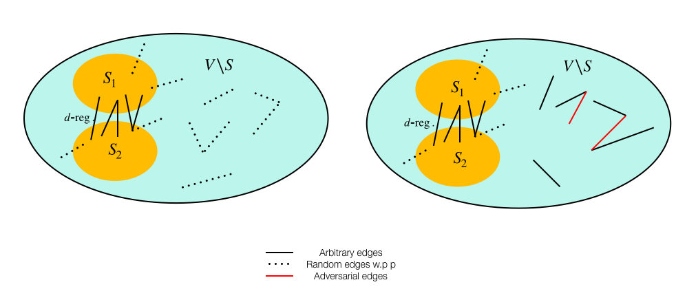
Figure 1: Random Planted model Definition 1 (left) and semi-random model Definition 2 (right).

We start by introducing our semi-random model which attempts to robustify the random planted model from Definition 1.

Definition 2 (Semi-random model).

Fix $n,k,d,p$, we now describe how a graph $G$ from our semi-random model is generated as,

1. Let $V$ be a set of $n$ vertices. Fix an arbitrary subset $S\subset V$ such that $\left\lvert S\right\rvert=k$.

2. Add edges arbitrarily inside $S$ such that the resulting graph is a connected $d$-regular bipartite graph. Let $S_{1},S_{2}$ denote the bipartite components.

3. For each pair of vertices in $S\times\left(V\setminus S\right)$, add an edge independently with probability $p$.

4. Arbitrarily add edges in $\left(V\setminus S\right)\times\left(V\setminus S\right)$ such that smallest eigenvalue of the matrix $\left(A_{\left(V\setminus S\right)\times\left(V\setminus S\right)}-p\mathbbm{1}_{V\setminus S}\mathbbm{1}_{V\setminus S}^{T}\right)$ is greater than $-\left((1/2-\alpha)/(1/2+\alpha)\right)d$ where $\alpha$ is a small positive constant (throughout this paper we assume $\alpha\leqslant 1/6$).

5. Allow a monotone adversary to add edges in $\left(V\setminus S\right)\times\left(V\setminus S\right)$ arbitrarily.

Observation 3.

Definition 2 also captures Definition 1; since in the case when $V\setminus$S is chosen to be a $G_{\left(n-k\right),p}$ random graph, $\left(A_{\left(V\setminus S\right)\times\left(V\times S\right)}-p\mathbbm{1}_{V\setminus S}\mathbbm{1}_{V\setminus S}^{T}\right)=A_{\left(V\setminus S\right)\times\left(V\setminus S\right)}-\operatorname*{\mathbb{E}}\left[A_{\left(V\setminus S\right)\times\left(V\setminus S\right)}\right]$, and therefore the smallest eigenvalue of $\left(A_{\left(V\setminus S\right)\times\left(V\times S\right)}-p\mathbbm{1}_{V\setminus S}\mathbbm{1}_{V\setminus S}^{T}\right)$ is greater than $-2\sqrt{n}$ (as follows from the work [Vu07]).

Models stronger than random planted models have also been considered in the literature for planted problems. The work [FK00] studies the planted clique problem in what they call the sandwich model. The model is constructed as per the random planted model in Definition 1, but an adversary is allowed to act on the top of that in a fashion similar to step 5 of Definition 2.

The work [FK01] introduced a strong adversarial semi-random model (referred to as the Fiege and Kilian model). They gave recovery algorithms for the planted clique ($k=\Omega(n)$ regimes) and for the planted bisection and planted $k$-coloring in this model. The work [MMT20] further shows that one can recover the planted clique for $k=\Omega_{p}\left(n^{2/3}\right)$ in [FK01] model.

In the Feige-Kilian model, step 4 allows for any arbitrary graph in $\left(V\setminus S\right)\times\left(V\setminus S\right)$. However, with no further assumptions on graph induced on $V\setminus S$, even for the special case of planted independent set problem ($d=0$), the best known algorithm [MMT20] works only for $k=\Omega_{p}\left(n^{2/3}\right)$. However, since our benchmark is $k=\Omega\left(\sqrt{n}\right)$, we look at a model with stronger assumptions than the Feige-Kilian model. In order to uniquely identify the planted graph, we need to assume that $V\setminus S$ is far from having any induced bipartite subgraphs of degree at least $d$. Our condition in step 4 implies that this indeed holds. This is because if the smallest eigenvalue is greater than $-d/2+2\sqrt{n}$, the graph is indeed far from having an induced bipartite subgraph of smallest degree $d$. Since otherwise, a vector having entries $1$ for one side of the bipartition and $-1$ on the other side and $0$ elsewhere achieves a Rayleigh Quotient of value $-d$ (and hence the smallest eigenvalue is at most $-d$).

We now present our main result which holds for both the random planted model (Definition 1) and semi-random model (Definition 2).

Theorem 4 (Informal version of Theorem 17 ).

For $n,k,d,p$ satisfying $k=\Omega_{p}\left(\sqrt{n\log n}\right)$ and $p=\Omega\left(\log k/k\right)^{1/6}$ and $d\geqslant 2pk/3$, there exists a deterministic algorithm that takes as input an instance generated by Definition 2, and recovers the arbitrary planted set $S$ exactly, in polynomial time and with high probability (over the randomness of the input).

Achieving exact recovery for $k=\Omega_{p}\left(\sqrt{n}\right)$ is still an open problem. To the best of our knowledge, nothing is known about this problem in full generality. For the planted clique problem, recovery for $k=\Omega\left(\sqrt{n\log n}\right)$ is trivial [Kuc95]. However, such techniques don’t work for our problem when $d=pk$. We prove Theorem 4 by showing that an SDP relaxation for the problem is integral, by constructing an optimal dual solution. We give an outline of the proof in Section 1.4 and a detailed proof in Section 2.

Our proofs use the spectral properties of bipartite graphs and random graphs to show the existence of an optimal dual solution having large rank. Our main technical contribution is a new approach for constructing a dual solution where we calibrate the eigenvectors of the adjacency matrix to be the eigenvectors of the dual matrix. We believe that this approach may have applications to other recovery problems in semi-random models as well.

Theorem 5 (Informal version of Theorem 37).

For $n,k,d,p$, satisfying $k=\Omega_{p}\left(\sqrt{n}\right)$, there exists a deterministic algorithm that takes as input an instance generated as per Definition 1, and recovers the arbitrary planted set $S$ exactly with high probability (over the randomness of the input) in time exponential in the number of small eigenvalues of the adjacency matrix (eigenvalues smaller than $-d/2+2\sqrt{n}$) of the graph induced on $S$.

Observation 6.

For and many special classes of instances such as, (i) when the probability $p=\Omega\left(1\right)$, (ii) when the planted graph is a complete bipartite graph like in the balanced biclique problem (iii) when the planted bipartite graph is a $d$-regular random graph or (iv) more generally when the planted graph is a $d$-regular expander graph; the number of these small eigenvalues is a constant in the regimes of $d=\Omega(pk)$ and Theorem 5 allows efficient recovery (running time of the algorithm is polynomial in $n$).

1.2 Related Work

Odd Cycle Transversal problem

The odd cycle transversal problem asks to find the smallest set of vertices in the graph such that the set has an intersection with every odd cycle of the graph. Removing these vertices will result in a bipartite graph, and hence this problem is equivalent to finding the largest induced bipartite graph. Owing to the hereditary nature of the bipartiteness property, the problem is NP-hard, as follows from the work of Yannakakis [Yan78]. The work [Yan78] shows that for a broad class of problems that have a structure that is hereditary on induced subgraphs, finding such a structure is NP-Complete. The optimal long code test by Khot and Bansal [BK09] rules out any constant factor approximation for this problem. On the algorithmic front, casting the problem as a $2$-CNF deletion problem, [AKRR90] gives a reduction to the min-multicut problem. This reduction gives us an $\mathcal{O}\left(\log n\right)$ approximation due to the work [GVY98], which was further improved to $\mathcal{O}\left(\sqrt{\log n}\right)$ in the work [ACMM05]. The work [GL21] gives an efficient randomized algorithm that removes only $\mathcal{O}\left(n\sqrt{{\sf OPT}\log d}\right)$ vertices where $d$ is the bound on the maximum degree of the graph and ${\sf OPT}$ denotes the fraction of vertices in the optimal set. They also give a matching (up to constant factors) Unique Games hardness for certain regimes of parameters.

The problem is equivalent to finding the largest 2-colorable subgraph of a given graph and is known as the partial 2-coloring problem. The work [GLR19] studies the problem in the Feige-Kilian semi-random model [FK01], where a 2-colorable graph of size $\left(1-\varepsilon\right)n$ is planted. They give an algorithm that outputs a set $\mathcal{S}^{\prime}$ such that $\left\lvert\mathcal{S^{\prime}}\right\rvert\geqslant\left(1-\varepsilon c/p^{2}\right)n$ for $p=\Omega\left(\sqrt{\log n/n}\right)$ and $\varepsilon\leqslant p^{2}$ where $c$ is a positive constant. Their algorithm is a partial recovery algorithm and works for the regimes when $\varepsilon$ is small. Our results in Theorem 4 hold when $1-\varepsilon$ is small and give complete recovery for a large range of $p$. However, since our model in Definition 2 makes stronger assumptions than the [FK01] model, we don’t make any comparisons.

Balanced Biclique problem

In the balanced complete bipartite subgraph problem (also called the balanced biclique problem), we are given a graph on $n$ vertices and a parameter $k$, and the problem then asks whether there is a complete bipartite subgraph that is balanced with $k$ vertices in each of the bipartite components. The problem was studied when the underlying graph is a bipartite graph, and shown to be NP-complete by a reduction from the CLIQUE problem in the works [GJ79, Joh87]. They additionally note that the balanced constraint is what makes the problem hard. If we remove the balanced constraint, the problem can be reduced to finding a maximum independent set in a bipartite graph. The latter problem admits a polynomial-time solution using the matching algorithm. The work [FK04] shows that this problem of finding a maximum balanced biclique is hard to approximate within a factor of $2^{\left(\log n\right)^{\delta}}$ for some $\delta>0$, under the assumption that $\mathsf{3SAT}\notin\textsf{DTIME}\left(2^{n^{3/4+\varepsilon}}\right)$ for some $\varepsilon>0$. Recently, the work [Man17] showed that one cannot find a better approximation than $n^{1-\varepsilon}$, assuming the Small Set Expansion Hypothesis and that $\textsf{NP}\nsubseteq\textsf{BPP}$ for every constant $\varepsilon>0$.

A related problem is the maximum edge biclique problem, where we are asked to find whether $G$ contains a biclique with at least $k$ edges. This problem was also shown to be NP-hard in the work [Pee03].

Given these intractability results for general graphs, there has been some success in special classes of graphs. In graphs with constant arboricity, the work [Epp94] gives a linear time algorithm that lists all maximal complete bipartite subgraphs. In a degree bounded graph, the work [TSS02] gives a combinatorial algorithm for the balanced biclique problem that runs in time $\mathcal{O}\left(n2^{d}\right)$. Another systematic approach, however, is to consider planted and semi-random models for the problem. In the work [Lev18], they study the planted version of the problem, which, they call hidden biclique problem. Their model is similar to our model in Definition 1; however, we consider an arbitrary $d$-regular bipartite graph instead of a complete bipartite graph. They give a linear-time combinatorial algorithm that finds the planted hidden biclique with high probability (over the randomness of the input instance) for $k=\Omega\left(\sqrt{n}\right)$. Their algorithm builds on the Low Degree Removal algorithm, due to Feige and Ron [FR10] which finds a planted clique in linear time.

Graph problems in Semi-random and Pseudorandom models

A wide variety of random graph models and their relaxations have been a rich source of algorithmic problems on graphs. Alon and Kahale [AK97] sharpened the results of Blum and Spencer [BS95] and gave algorithms that recover a planted $3$-coloring in a natural family of random $3$-colorable instances. [KLT17] extended this result and showed how to recover a $3$-coloring when the input graph is pseudorandom (has some mild expansion properties) and is known to admit a random like $3$-coloring. A unified spectral approach by McSherry [McS01] gives a single shot recovery algorithm for many problems in these random planted models. One can use the [McS01] framework to recover a planted random bipartite graph; however, it is not known if it will work if $S$ is an arbitrary bipartite graph.

On the other side, we have semi-random models. Notably, the Feige-Kilian model [FK01] is one of the strongest semi-random models. In [FK01], they also give recovery algorithms for planted clique, planted $k$-colorable, and planted bisection problem in this model. In [MMT20], they give a recovery algorithm for the independent set problem for large regimes of parameters. The work [KLP21] generalizes these results to $r$-uniform hypergraphs in this model. There are other works [MMV12, MMV14, LV18, LV19] that study graph partitioning in semi-random models.

A host of work has been done in various random and semi-random models for the more general densest $k$-subgraph problem. The works by Hajek, Wu, and Xu [HWX16a, HWX16b, HWX16c] study the problem when the planted dense subgraph is random and gives algorithms for exact recovery using SDP relaxations for some range of parameters. They complement these results by providing information-theoretic limits for regimes where recovery is impossible. The work by [BCC⁺10] studies this problem when the planted graph is arbitrary. They analyze an SDP-based method to distinguish the dense graphs from the family of $G_{n,p}$ graphs when $k\geqslant\sqrt{n}$. The work [KL20] studies the problem of densest $k$-subgraph in some semi-random model and gives a partial recovery algorithm for some regimes of $d,k,n,p$.

SDP has been the tool of choice for exact recovery in semi-random models. Starting from the fundamental works of exact recovery for the planted clique problem [FK00], for the planted bisection problem [FK01], for Stochastic Block Models [ABH16] etc., (and many other works as have been mentioned above), are based on SDP relaxations. A natural way to analyze these SDP relaxations is by constructing an optimal dual solution to prove integrality of the primal relaxation. This idea has been explored in the works of [FK01, CO07, BCC⁺10, ABBS14, ABH16, LV18], to state a few. We note that the task of constructing an optimal dual solution is problem-specific, and there is no generic way of doing this.

1.3 Preliminaries

We start with some essential notation to understand the proof overview and review some well-known facts about random perturbation matrices. Then, we write our SDP relaxation to the problem and the accompanying dual SDP. We follow this up with a discussion on some well known tools from spectral graph theory such as the threshold rank and spectral embedding. We will build on these ideas in our Proof Overview Section 1.4 to show that the primal SDP is an optimal one and the primal matrix is a rank-one matrix.

1.3.1 Notation

We let $\left[M\right]_{n\times n}$ denote a matrix $M$ of size $n\times n$. For some set of indices $R_{1},R_{2}\subseteq[n]$, $M_{R_{1}\times R_{2}}$ denotes a matrix of size $n\times n$ constructed out of matrix $M$ of size $n\times n$ by copying the entries for $(i,j)\in R_{1}\times R_{2}$ and setting rest of the entries to be $0$. We let $\left.M\right|_{R_{1}\times R_{2}}$ denote the matrix of size $\left\lvert R_{1}\right\rvert\times\left\lvert R_{2}\right\rvert$ constructed from a matrix $M$ of size $n\times n$ by taking rows corresponding to $R_{1}$ and columns corresponding to $R_{2}$. The eigenvalues of a matrix $M$ are sorted as $\lambda_{1}(M)\leqslant\lambda_{2}(M)\leqslant\ldots\leqslant\lambda_{n}(M)$. We will drop the matrix $M$ wherever it is clear from the context. The eigenvectors are also sorted by their corresponding eigenvalues.

1.3.2 Spectral bounds on Perturbation matrices

We let $A$ denote the adjacency matrix of the graph obtained using Definition 1. We can express the matrix $A$ as sum of simpler matrices,

$$A=A_{S\times S}+A_{V\setminus S\times V\setminus S}+p\left(\mathbbm{1}\mathbbm{1}^{T}-\mathbbm{1}_{S}\mathbbm{1}_{S}^{T}-\mathbbm{1}_{V\setminus S}\mathbbm{1}_{V\setminus S}^{T}\right)+R \left(R_{ij}\stackrel{{\scriptstyle\textup{def}}}{{=}}A_{ij}-\operatorname*{\mathbb{E}}[A_{ij}]\right)$$ (1)

where $A_{S\times S}$ represents the matrix corresponding to the planted bipartite graph, the term $p\left(\mathbbm{1}\mathbbm{1}^{T}-\mathbbm{1}_{S}\mathbbm{1}_{S}^{T}-\mathbbm{1}_{V\setminus S}\mathbbm{1}_{V\setminus S}^{T}\right)$ is the expected adjacency matrix for the random graph and $R$ as defined above is the perturbation matrix corresponding to the random part of the graph.

Proposition 7.

For the perturbation matrix $R$ as defined in equation (1) we have that $\left\lVert R\right\rVert\leqslant 2\sqrt{n}$ almost surely.

Proof.

$R$ is a symmetric random matrix and the entries $R_{ij}$ can be treated as random variables, bounded between $-1$ and $1$, with expectation $0$ and variance $p\left(1-p\right)\leqslant 1/4$. Also the entries $R_{ij}$ are independent and hence, by Theorem 1.1 in the work [Vu07], we have $\left\lVert R\right\rVert\leqslant 2\sqrt{n}$ almost surely. ∎

1.3.3 SDP Relaxation

Our main results are based on analyzing the following SDP relaxation SDP 8. We construct its dual SDP 9 (refer to Appendix A.1 for more details on this dual construction).

In SDP 9, the Lagrange multipliers $\beta_{i}$’s,$\gamma_{i}$’s and $B_{ij}$’s are our dual variables and $Y$ is the dual SDP matrix. By $\mathbbm{1}_{ij}$ we mean an indicator matrix which is one for $(i,j)$ entry and zero elsewhere. Similarly, $D_{i}$ is an indicator matrix which is one for $(i,i)$ entry and zero elsewhere. For clarity, we will denote $\sum_{\left\{i,j\right\}\in E}B_{ij}\left(\mathbbm{1}_{ij}+\mathbbm{1}_{ji}\right)$ by a matrix $B$.

Intended solution:

We denote the primal SDP matrix by $X$ and let $\mathbf{x}_{i}$ denote the vector corresponding to vertex $i$ such that $X_{ij}=\left\langle\mathbf{x}_{i},\mathbf{x}_{j}\right\rangle$.

Our intended integral solution to the SDP is $X=\mathbf{g}\mathbf{g}^{T}$, where $\mathbf{g}\in\mathbb{R}^{n}$ s.t $g_{i}=1/\sqrt{k}$ for $i\in S_{1}$, $g_{i}=-1/\sqrt{k}$ for $i\in S_{2}$ and $0$ otherwise. This solution is obtained by setting,

$$\mathbf{x}_{i}^{*}=\begin{cases}\hat{e}/\sqrt{k}&\text{if }i\in S_{1}\\ -\hat{e}/\sqrt{k}&\text{if }i\in S_{2}\\ 0&\text{otherwise},\end{cases}$$ (8)

where $\hat{e}$ is some unit vector.

Weak Duality for fixing dual variables:

Let $\mathsf{SDPOPT}\left(G\right)$ denote the optimal value of the primal SDP; then from the proposed integral solution we have that,

$$\mathsf{SDPOPT}\left(G\right)\leqslant-2\sum_{\left\{i,j\right\}\in E}\left\langle\mathbf{x}_{i}^{*},\mathbf{x}_{j}^{*}\right\rangle=\left\langle A,\mathbf{g}\mathbf{g}^{T}\right\rangle=\mathbf{g}^{T}A\mathbf{g}=-d\,.$$

For any feasible solution to the dual SDP 9, by weak duality, we know that

$$\beta-\sum_{i\in V}\gamma_{i}\leqslant\mathsf{SDPOPT}\left(G\right)\leqslant-d\,.$$

We note that the upper bound is achievable by setting $\beta=-d$ and $\gamma_{i}=0,\forall i\in V$.

We will show later that the remaining dual variables $B_{ij}$’s can be chosen in a way that the choice of $\beta=-d$ and $\gamma_{i}=0,\forall i\in V$ yields a feasible dual solution.

Fact 10 (Foklore, also see Lemma 2.3 in [LV18]).

The primal solution $X=\mathbf{g}\mathbf{g}^{T}$ is the unique solution to SDP 8 if there exists a dual matrix $Y$ such that it satisfies constraints in SDP 9, with $\beta=-d$ and $\gamma_{i}=0,\forall i\in V$ and having ${\sf rank}(Y)=n-1$ (i.e. $\lambda_{2}\left(Y\right)>0$).

Proof.

For completeness, we give a proof in Appendix A.3. ∎

1.3.4 Threshold rank eigenvectors:

Definition 11 (Threshold rank of a graph).

For $\tau\in[0,d]$, we define threshold rank of a graph with adjacency matrix $G$ (denoted by ${\sf rank}_{\leqslant-\tau}(G)$) as,

$${\sf rank}_{\leqslant-\tau}(G)=\left\lvert\left\{i:{\lambda_{i}(G)}\leqslant-\tau\right\}\right\rvert\,.$$

We let $P_{-\tau}=\left\{\mathbf{v}^{\left(1\right)},\mathbf{v}^{\left(2\right)},\ldots,\mathbf{v}^{\left(L_{-\tau}\right)}\right\}$ (the bottom $L_{-\tau}$ vectors) denote the set of orthonormal eigenvectors of $\left.{A}\right|_{{S\times S}}$ with eigenvalues smaller than the threshold $-\tau$, breaking ties arbitrarily where $L_{-\tau}={\sf rank}_{\leqslant-\tau}\left(\left.{A}\right|_{{S\times S}}\right)$. We call these vectors as $\tau$-threshold rank eigenvectors of $\left.{A}\right|_{{S\times S}}$. Next, we recall a well known fact about the threshold rank of a graph.

Fact 12 (Folklore).

${\sf rank}_{\leqslant-\tau}\left(\left.A\right|_{S\times S}\right)\leqslant\dfrac{kd}{2{\tau}^{2}}$.

Proof.

Since, $\left.{A}\right|_{{S\times S}}$ is the adjacency matrix of a bipartite graph, it’s eigenvalue spectrum is symmetric around $0$. Therefore the number of eigenvalues with absolute value greater then or equal to $\tau$ is given by $2\,{\sf rank}_{\leqslant-\tau}\left(\left.{A}\right|_{{S\times S}}\right)$ and are bounded as,

$$2{\tau}^{2}{\sf rank}_{\leqslant-\tau}(\left.{A}\right|_{{S\times S}})\leqslant\sum_{i}{\lambda_{i}^{2}(\left.{A}\right|_{{S\times S}})}\leqslant\left\lVert\left.{A}\right|_{{S\times S}}\right\rVert^{2}_{F}=kd.$$

∎

We note that a similar notion of threshold rank has appeared in other works [ABS10, AG11, BRS11, GT13] etc.

1.3.5 Spectral embedding vectors:

Definition 13 (Spectral embedding vectors).

Given the planted bipartite graph $S$ and the matrix of bottom $L_{-\tau}$ orthonormal eigenvectors $W^{T}_{-\tau}=\begin{bmatrix}\mathbf{v}^{\left(1\right)}&\mathbf{v}^{\left(2\right)}&\ldots&\mathbf{v}^{\left(L_{-\tau}\right)}\end{bmatrix}$, we define the spectral embedding of a vertex $i\in S$ as the $L_{-\tau}$-dimensional vector given by $\mathbf{w}^{\left(i\right)}=W_{-\tau}\mathbf{e}_{i}$ where $\mathbf{e}_{i}$ is a vector with one in the $i^{th}$ coordinate and zero elsewhere.

Informally, these are the vectors obtained by looking at the subspace of the columns of $W^{T}_{-\tau}$ where the vertex $i$ is mapped to the $i^{th}$ column of $W^{T}_{-\tau}$. These spectral embedding vectors have been explored in various works on graph partitioning as [NJW01, LOGT12, LRTV12] etc. It is known that these spectral embedding vectors are well spread, formally referred to as being in an isotropic position. We define these set of vectors to be in an isotropic position if $\sum_{i\in S}\mathbf{w}^{(i)}=0$ and $\sum_{i\in S}\mathbf{w}^{(i)}{\mathbf{w}{{}^{(i)}}^{T}}=I$ where $I$ is an $L_{-\tau}\times L_{-\tau}$ sized identity matrix. The condition that $\sum_{i\in S}\mathbf{w}^{(i)}{\mathbf{w}{{}^{(i)}}^{T}}=I$ can equivalently be written as $\sum_{i\in S}\left\langle\mathbf{y},\mathbf{w}^{(i)}\right\rangle^{2}=1,\forall\mathbf{y}\text{ with }\left\lVert\mathbf{y}\right\rVert_{2}=1$.

Lemma 14 (Folklore).

The spectral embedding vectors are in an isotropic position.

For a proof, we refer the reader to the work [LRTV11].

1.4 Proof Overview

For the sake of simplicity, we will assume that the graph is sampled as per the random planted model (Definition 1). We will also allow an action of a monotone adversary (as in step 5) on this model; but we analyze its action separately (in Section 1.4.6). The main ideas for the semi-random model (Definition 2) are essentially the same, and the additional steps to handle them is just a technical adjustment.

1.4.1 Spectral Approaches

We start with some natural spectral approaches for recovering the planted set. These approaches have found some success, e.g. in recovering planted cliques/independent sets, planted bisection, planted $k$-colorable graphs (refer work [McS01] for details). We recall from our earlier discussion, that the interesting regimes for this problem are $k=\Omega\left(\sqrt{n}\right)$ and $d\approx pk$.

Detecting planted bipartitions and why it is easy:

We note that the detection problem i.e. detecting the presence of bipartite graph as constructed in the random planted model (Definition 1) against the null hypothesis of Erdős-Rényi graph $G_{n,p}$, is easy when $k=\Omega\left(\sqrt{n}\right)$. Formally one notes that given two distributions

$$H_{0}:G\sim G\left(n,p\right)\text{ against }H_{1}:G\sim G\left(n,k,d,p\right)\text{ as per \hyperref@@ii[def:planted_model]{Definition~{}\ref*{def:planted_model}}},$$

the spectral test, which outputs $H_{1}$ when $\lambda_{1}\left(G\right)\leqslant-d$ and $H_{0}$ otherwise, is correct almost surely for $d\approx pk$ and $k\geqslant c\sqrt{n}/p$ where $c>0$ is a large enough constant. This is because for a $G_{n,p}$ graph, the smallest eigenvalue is greater than $-2\sqrt{n}$ almost surely (Claim 7), while for a graph with planted bipartite subgraph, the smallest eigenvalue is smaller than $-d$ since the vector $\mathbbm{1}_{S_{1}}-\mathbbm{1}_{S_{2}}$ already achieves Rayleigh Quotient of value $-d$.

The challenges in exact recovery:

However, as expected, the exact recovery problem is more challenging. There are some works that look at these planted problems on an individual basis ([Bop87],[AKS98]). They typically rely on the spectral bounds of perturbation matrices and the framework of Davis-Kahan theorem (refer [Ver18]) to identify eigenvector(s) indicating the planted set. However, we need a sufficient eigengap to apply these results from perturbation theory. Since our planted graph $S$ in the random planted model is an arbitrary bipartite graph, it can have any number of eigenvalues close to the smallest eigenvalue $-d$ and hence we may not have such an eigengap.

A unified spectral framework for random planted models was given by McSherry [McS01] (further refined in the work [Vu18]). Here, one can check that we cannot satisfy the conditions in Observation 11 of this work [McS01] if the planted set has size $o(n)$. Again, the reason is because the planted bipartite graph is arbitrary. Since the planted bipartite graph can have arbitrary rank we cannot get the constants $\gamma_{1}$ in [McS01] to be small enough to recover in $o(n)$ regimes. It is also easy to verify that this framework works if the planted bipartite graph is also a random graph, for regimes of $k=\Omega\left(\sqrt{n}\right)$ and $d\approx pk$ (say by choosing edge probability for the random planted bipartite graph as $p^{\prime}=2p$).

A subspace enumeration style approach:

Another spectral approach, inspired from the works of [KT07, ABS10, Kol11, KLT17] is to apply the subspace enumeration technique to recover a large fraction of planted set $S$. Here we first identify (in Lemma 41) that the vector $\mathbf{u}=\mathbbm{1}_{S_{1}}-\mathbbm{1}_{S_{2}}$ has a large projection on the space spanned by $\tau^{\prime}$-threshold rank eigenvectors of $A$ (for choice of $\tau^{\prime}=d/2$). Note that this vector $\mathbf{u}$ identifies the planted set (as well as the planted bipartition), and therefore we call it the signed indicator vector. We then do a standard $\varepsilon$-net construction to find a vector $\mathbf{y}$ close to $\mathbf{u}$ and use $\mathbf{y}$ to recover a large fraction of planted set $S$ (Lemma 42 and Lemma 38). We can recover the remaining set of vertices by an argument due to the work [GLR19] (Lemma 43), where they distinguish vertices by the size of matching in induced neighborhoods. Putting all this together, we can prove Theorem 5.

The running time of the procedure described above is exponential in $L_{-\tau}$ where $L_{-\tau}=\mathcal{O}\left(1/p\right)$ for $\tau=\Omega\left(d\right)$ (follows from Lemma Fact 12). Therefore, for many special classes of instances such as, (i) when the probability $p=\Omega(1)$ and $d=\Omega(pk)$, (ii) when the planted graph is a complete bipartite graph (this is the balanced biclique problem) and $d=\Omega(pk)$, (iii) when the planted bipartite graph is $d$-regular random graph for $d=\Omega(pk)$ or (iv) more generally when the planted graph is a $d$-regular expander graph for $d=\Omega(pk)$ we have $L_{-\tau}=\mathcal{O}\left(1\right)$ and this already gives us a polynomial-time algorithm.

However, as stated earlier, we want to solve the problem in $p=o(1)$ regimes. To accomplish this, we shift our focus to the SDP formulation we mentioned in SDP 8. Also, for other problems in this literature (planted clique, planted bisection, planted $k$-colorable, Stochastic Block models etc), only SDP’s have provable guarantees of working in the presence of such monotone adversaries (refer Chapter 10 in [Rou21] for more intuition on this).

1.4.2 Traditional SDP Analysis

Now we overview our SDP-based approach to solving the problem. We will see that the difficulties in the spectral approach will translate to showing the feasibility of the dual SDP solution. However, we have more freedom here since we have the dual variables to work with and we can use them and try to enforce the optimality of the dual solution.

Characterizing dual variables through optimality conditions:

A standard technique for analyzing SDP relaxations (like our SDP 8) is to show optimality by constructing a dual solution that matches the ${\sf SDPOPT}\left(G\right)$ value of the primal in a manner that the dual matrix $Y$ is positive semi-definite and has rank $n-1$, (see Fact 10).

These impose a wish list of desired conditions, which can be used to characterize our dual variables

1. $\beta=-d$ (Optimal objective)

2. $\left\langle\mathbf{g}\mathbf{g}^{T},Y\right\rangle=0$ (Complementary slackness)

3. $Y\succeq 0$ (Dual feasibility)

4. $\lambda_{2}\left(Y\right)>0$ (Strong duality).

Using weak duality we set $\beta=-d$ and $\gamma_{i}=0,\forall i\in V$ to match the optimal primal objective value of ${\sf SDPOPT}=-d$. We expand upon the complementary slackness condition as,

$$\left\langle\mathbf{g}\mathbf{g}^{T},Y\right\rangle=\mathbf{g}^{T}Y\mathbf{g}=\mathbf{g}^{T}\left(A+dI\right)\mathbf{g}+\mathbf{g}^{T}B\mathbf{g}=0+\mathbf{g}^{T}B\mathbf{g}=\mathbf{g}^{T}B\mathbf{g}\,.$$

Therefore the complementary slackness condition gives us that,

$$\sum_{i\in S}\sum_{\begin{subarray}{c}j\in S\\ \left\{i,j\right\}\in E\end{subarray}}B_{ij}=0$$ (9)

and since the SDP dual requires that $B_{ij}\geqslant 0$, it implies that $B_{ij}=0$ for all $(i,j)\in E(S_{1},S_{2})$. Now using the characterization of dual variables from conditions (1) and (2), one tries to show the feasibility of the dual and the strong duality rank condition. Typically, this characterization turns out to be rather weak. So, we refer to the dual variables set so far (ensuring condition (1) and (2) are satisfied) as weakly characterized.

Showing optimality of dual solution through weakly characterized dual variables

For certain problems in semi-random models, such as the planted clique problem [FK00], community detection in SBM [ABH16], the weak characterization above suffices. We are able to show that the weakly characterized dual solution satisfies conditions (3) and (4). This is typically done by invoking some standard results for random matrix bounds and concentration inequalities. In our setup, satisfying condition (3) requires that

$$\lambda_{\min}\left(Y\right)\geqslant 0\text{ which is implied if }\lambda_{\min}\left(A\right)+d+\lambda_{\min}\left(B\right)=\lambda_{\min}(A)+d\geqslant 0\,.$$ (10)

However, in our random planted model, the smallest eigenvalue of $A$ can be smaller than $-d-2\sqrt{pn}$ and condition (3) may not hold (as per choice of $B_{ij}$’s dictated from equation (9)). Thus we need a stronger characterization of dual variables to satisfy the conditions (3) and (4). In our problem, we need to make use of the large number of unused dual variables $B_{ij}^{\prime}s$ for $\left\{i,j\right\}\in E\cap\left\{\left(V\times V\right)\setminus\left(S\times S\right)\right\}$

Guessing/Constructing the dual certificate

Now we discuss an approach of making the dual matrix satisfy conditions (3) and (4) by guessing the dual variables thus giving an explicit setting of dual variables. This is typically done by assigning some sort of meaning to dual variables and guessing their values based on the input instance. This approach has found reasonable success in other recovery problems like the planted bisection problem [FK01], coloring semi-random graphs [CO07], decoding binary node labels from censored edge measurements [ABBS14], and planted sparse vertex cuts [LV18].

Therefore, we may expect to guess a nice setting of dual variables that satisfy equation (10). However, if one takes a deeper look at this approach, the task again reduces to applying results from perturbation theory. Again, such an approach would work if the planted bipartite graph were also a random graph or an expander, since there would only be a single eigenvector whose corresponding eigenvalue disobeys equation (10), and one could choose the dual variables constructively to handle it and make it satisfy condition (3).

However, for an arbitrary planted bipartite graph, we can have a lot of eigenvalues in the interval $[-d,-d-2\sqrt{n}]$ (and hence the entire graph $A$ can have a lot of eigenvalues in the interval $[-d-2\sqrt{n},-d]$). Therefore, we need a more principled approach to deal with the corresponding eigenvectors of the planted graph having eigenvalue close to $-d$ (as we pointed out earlier, there can be $\mathcal{O}\left(1/p\right)$ such eigenvectors).

1.4.3 Calibrating the eigenvectors

Now we present our approach towards satisfying conditions (3) and (4), which is to calibrate the eigenvectors. We will see that, this calibration will further complicate our requirements on the dual variables, however we will argue in Section 1.4.4 on how we manage that.

Obtaining optimality of Primal SDP by assuming existence of a certifying $B$:

It is now clear that our Achilles’ heel are the eigenvalues (and corresponding threshold rank eigenvectors) of the planted graph in the interval $[-d,-d-2\sqrt{n}]$. If we were allowed to ignore these vectors it’s easy to see that equation (10) and hence condition (3) holds.

Our core idea is to extend (by padding with $0$’s so that they are the right length) the threshold rank eigenvectors of $\left.{A}\right|_{{S\times S}}$ to be the eigenvectors of the dual matrix $Y$. Recall, the eigenvalues of $\left.{A}\right|_{{S\times S}}$ lie in the interval $\left[-d,d\right]$. Now take a threshold rank eigenvector of $\left.{A}\right|_{{S\times S}}$ (say with eigenvalue $\lambda_{l}$). We wish to calibrate such a threshold rank eigenvector to be an eigenvectors of $Y$ with eigenvalue $d+\lambda_{l}$. If we are able to achieve this calibration, we need not bother about the $2\sqrt{n}$ term since now these eigenvectors have a non-negative quadratic form.

The only thing at our disposal for this calibration are the unused (so far) dual variables $B_{ij}$’s. Denote this set of threshold rank eigenvectors of $\left.{A}\right|_{{S\times S}}$ as $P_{-\tau}$. Given this set $P_{-\tau}$, achieving this calibration can be expressed as satisfying the system of equations,

$$\sum_{i\in S}{\mathbf{v}^{\left(l\right)}_{i}\left(A_{ij}+B_{ij}\right)}=0,\quad\forall j\in V\setminus S,\forall\,\mathbf{v}^{\left(l\right)}\in P_{-\tau}\,.$$ (11)

• $L$ different system of equations $\mathcal{E}_{l}$, one for each $\mathbf{v}^{\left(l\right)}$.

• Each system $\mathcal{E}_{l}$ involves $|S|\times|V\setminus S|$ variables $B_{ij}$ where $i\in S$ and $j\in V\setminus S$.

Now, all we need is a setting of $B_{ij}$’s such that the system of equations is satisfied. However, this will still not be enough. We note that if this system of equations were to have a solution, we would have set some of these $B_{ij}$ variables to non-zero values. Therefore our equation (10) would now need to be modified to showing that $\lambda_{\min}\left(A\right)+d+\lambda_{\min}\left(B\right)\geqslant 0$.

The way we deal with this is by noting that we can tune $\tau>0$ apriori to be sufficiently large for this calibration such that $\lambda_{\min}(A)+d\geqslant\eta$ where $\eta>0$; and now impose an additional constraint on the matrix of dual variables that $\left\lVert B\right\rVert\leqslant\eta$. At this point, it seems highly suspicious as whether such $B_{ij}$’s exist. However, if we table these considerations aside and for choice of $\tau=2d/3$ and $\eta=\tilde{\mathcal{O}}\left(pk\right)$ we can indeed show that condition (3) and condition (4) of our wish list are met (Lemma 22) and we get the desired integral primal solution.

1.4.4 Setting of dual variables

In this section we show that there exists a matrix of non-negative dual variables $B_{ij}$’s that satisfies the system of equations (11) and $\left\lVert B\right\rVert_{2}=\tilde{\mathcal{O}}\left(pk\right)$.

An LP formulation and Farkas Lemma based approach.

We start by observing that the condition $\left\lVert B\right\rVert_{2}=\tilde{\mathcal{O}}\left(pk\right)$ is implied by a condition that $B_{ij}\leqslant t=\mathcal{O}_{p}\left(\sqrt{\log k/k}\right),\forall(i,j)\in\left(S\times\left(V\setminus S\right)\right)\cup\left(\left(V\setminus S\right)\times S\right)$ (Corollary 24). Also, since these system of equations (11) only concerns the non-negative dual variables $B_{ij}$’s with $\left\{i,j\right\}\in\left(S\times\left(V\setminus S\right)\right)\cup\left(\left(V\setminus S\right)\times S\right)$, we set the rest of them to $0$.

We now reorganize our collection of linear systems in (11) as follows.

• For $j\in V\setminus S$, define a system of equations $\mathcal{F}_{j}$.

• In all, this gives a collection of systems $\{\mathcal{F}_{j}\}_{j\in V\setminus S}$. Each system contains $L_{-\tau}\times|S|$ variables. In particular, the system $\mathcal{F}_{j}$ is expressed in the standard form $W_{-\tau}\mathbf{x}=\mathbf{b}$, where $W_{-\tau}\in\mathbb{R}^{L_{-\tau}\times k}$ is a matrix formed by stacking the vectors $\mathbf{v}^{\left(l\right)}\in P_{-\tau}$ as rows.

Fix $j\in V\setminus S$ and consider the system $\mathcal{F}_{j}$. The vector $\mathbf{b}$ in this system is a row vector of size $L_{-\tau}\times 1$ and has entries given by $b_{l}=-\sum_{i\in S}{A_{ij}v^{\left(l\right)}_{i}},\forall l\in[L_{-\tau}]$ and $\mathbf{x}$ here is a row vector of size $k\times 1$ where the entry $x_{i}=B_{ij}$ (recall that we have fixed a $j\in V\setminus S$). However since $B_{ij}$’s are not arbitrary variables but dual variables of SDP 9, these are required to be non-negative and should only be defined for $i\in N(j)$. Since the graph on $S\times\left(V\setminus S\right)$ is random, the choice of random edges while choosing $N(j)$ (in model construction) corresponds to setting those $B_{ij}=0$ whenever the edge is not chosen. Let $\tilde{W}_{-\tau}$ denote the submatrix after removing the columns corresponding to $i\notin N(j)$ and recall $t$ is our upper bound on the entries of $B$ matrix as mentioned above. We then consider the following feasibility LP formulation for this problem of finding appropriate $B_{ij}$’s.

For simplicity, consider the case $p=1$, i.e. when $A_{ij}=1$ for all $i\in S,j\not\in S$. Then we have that for any vector $\mathbf{y}\in\mathbb{R}^{L_{-\tau}}$,

$$\mathbf{b}^{T}\mathbf{y} =\sum_{r\in[L_{-\tau}]}b_{r}y_{r}=-\sum_{r\in[L_{-\tau}]}\sum_{i\in S}v^{\left(r\right)}_{i}y_{r}=-\sum_{i\in S}\sum_{r\in[L_{-\tau}]}v^{\left(r\right)}_{i}y_{r}$$ (14)

$$=-\sum_{i\in S}\sum_{r\in[L_{-\tau}]}w^{\left(i\right)}_{r}y_{r}=-\sum_{i\in S}\left\langle\mathbf{w}^{\left(i\right)},y\right\rangle=-\left\langle\sum_{i\in S}{\mathbf{w}^{\left(i\right)}},\mathbf{y}\right\rangle=0\,.$$ (15)

Using the standard variant of Farkas’ Lemma, this immediately implies the existence of a solution to equation (11). However, in general, for $p<1$, we need to do more work here.

We apply a more general version of Farkas’ Lemma (Corollary 27), and we have that satisfying this LP in the general case corresponds to showing that for some $t>0$, the following holds.

$$\forall\;\mathbf{y}\in\mathbb{R}^{L_{-\tau}},\forall\;\mathbf{z}\geqslant 0,\;\tilde{W}_{-\tau}^{T}\mathbf{y}+\mathbf{z}\geqslant 0\implies\mathbf{b}^{T}\mathbf{y}+t\left\langle\mathbf{z},\mathbbm{1}\right\rangle\geqslant 0\,.$$ (16)

The first term in the expression, $\mathbf{b}^{T}\mathbf{y}$, can be expanded as in equation (14) to obtain

$$\mathbf{b}^{T}\mathbf{y}=-\sum_{i\in N(j)}\left\langle\mathbf{w}^{\left(i\right)},\mathbf{y}\right\rangle\text{ and using }\left(\tilde{W}_{-\tau}^{T}\mathbf{y}\right)_{i}=\left\langle\mathbf{w}^{\left(i\right)},\mathbf{y}\right\rangle\text{ we have }z_{i}\geqslant-\left\langle\mathbf{w}^{\left(i\right)},\mathbf{y}\right\rangle.$$

We give a proof by contradiction (Proposition 30) for equation (16). By contradiction there exists a $\mathbf{y}$ and a $\mathbf{z}$ such that $\mathbf{b}^{T}\mathbf{y}+t\left\langle\mathbf{z},\mathbbm{1}\right\rangle<0$. We choose $\mathbf{z}^{\prime}\leqslant\mathbf{z}$ by setting $z^{\prime}_{i}=\max\left\{0,-\left\langle\mathbf{w}^{(i)}\right\rangle,\mathbf{y}\right\}$ and argue that it is enough to show contradiction for $t,\mathbf{y}$ and $\mathbf{z}^{\prime}$. Using the expressions for $\mathbf{b}^{T}\mathbf{y}$ as above, this translates to showing that

$$\sum_{i\in N(j)}\left\langle\mathbf{w}^{\left(i\right)},\mathbf{y}\right\rangle+t\sum_{i\in N(j)}{\min\left\{0,{\left\langle\mathbf{w}^{\left(i\right)},\mathbf{y}\right\rangle}\right\}}>0,$$ (17)

has no solution. We show that equation (17) does not hold for our desired choice of $t=\mathcal{O}_{p}\left(\sqrt{\log k/k}\right)$.

We note that the second term in equation (17) is $\geqslant 0$, and we wish the inequality to not hold for as small a value of $t$ as possible; therefore, we seek an upper bound on both terms.

Structure of threshold rank/spectral embedding vectors.

To upper bound the first term, it might be helpful to understand the structure of the spectral embedding vectors $\mathbf{w}^{\left(i\right)}$. Since these are intimately connected to the threshold rank eigenvectors $\mathbf{v}^{\left(l\right)}$, we use these eigenvectors to characterize them. For convenience we let $\mathbf{v}^{\left(l\right)}\in P_{-\tau}$ have unit norm, then in Lemma 28 we show that $\left\lVert\mathbf{v}^{\left(l\right)}\right\rVert_{\infty}=\left\lVert\mathbf{w}^{\left(i\right)}\right\rVert_{\infty}\leqslant 2/\sqrt{d}$. Since $i\in N(j)$ are sampled randomly, we can use the Hoeffding bounds to upper bound the $l_{\infty}$ norm for $\sum_{i\in N(j)}\mathbf{w}^{\left(i\right)}$ and hence upper bound our first term (Lemma 29) by $\mathcal{O}_{p}\left(\sqrt{\log k}\right)$ with high probability. We choose our parameters such that the vectors in $P_{-\tau}$ are orthogonal to $\mathbbm{1}_{S}$. For the embedding vectors, this translates to saying that $\sum_{i\in S}\mathbf{w}^{\left(i\right)}=0$.

Towards bounding the second term, we use these spectral embedding vectors. The spectral embedding vectors are isotropic for $p=1$ (already where we can easily show that equation (17) does not hold and we are done). However, for $p<1$, we have $i\in N(j)$ (and corresponding embedding vectors) being sampled randomly as per $G_{n,p}$ distribution. Here, in Lemma 31, we show that by using Matrix Bernstein concentration we can get close to isotropic vectors,

$$\sum_{i\in N(j)}\left\langle\mathbf{y},\mathbf{w}^{\left(i\right)}\right\rangle^{2}\geqslant p/2 \left(\text{This shows that embedding vectors are $p/2$-isotropic }.\right)$$ (18)

Showing existence of a solution to LP 15.

Now, we look at two cases; the first case where the negative terms dominate the summand in equation (17), then we use the eigenvector structure that $\left\lVert\mathbf{w}^{\left(i\right)}\right\rVert\leqslant 2/\sqrt{d}$ and we are done; for the other case where the positive terms dominate, we relate the positive terms to the negative terms again using the bound we obtained from the eigenvector structure $\left\lVert\sum_{i\in N(j)}\mathbf{w}^{\left(i\right)}\right\rVert=\mathcal{O}_{p}\left(\sqrt{\log k}\right)$.

Therefore, we argue in Lemma 34, that we can upper bound the second term by $-\Omega_{p}\left(\sqrt{k}\right)$. Therefore using these bounds we show in Proposition 30, that for a choice of $t$ as we obtained above of $t=\mathcal{O}_{p}{\left(\sqrt{\log k/k}\right)}$, equation (17) does not hold. As discussed earlier this implies that the there exists a dual such that conditions (1)-(4), equation (11) and $\left\lVert B\right\rVert_{2}=\tilde{\mathcal{O}}\left(pk\right)$ holds which further implies that the primal SDP is feasible. Further, if the graph is connected; the signed indicator vector would be the only eigenvector with eigenvalue $-d$ (after padding to make these the eigenvectors of $Y$), this would be the only eigenvector of $Y$ with eigenvalue $0$. Using Fact 10, this implies that the proposed integral solution in equation (8) is the only integral solution and hence Cholesky Decomposition of our SDP matrix returns the signed indicator vector and thus our planted set.

1.4.5 Low degree regimes

The discussion above about SDP holds only where $d=\gamma pk$ where $\gamma\geqslant 2/3$. Note that this covers our interesting regimes when $d\approx pk$ where the problem is non-trivial. The other case where $d\leqslant 2pk/3$, can actually be trivially solved for $k=\Omega_{p}\left(\sqrt{n\log n}\right)$ using a degree counting argument along the lines of [Kuc95] as we discuss below.

Now we consider the regimes when $d=\gamma pk$ with $\gamma\leqslant 2/3$. We show that a simple algorithm that collects the bottom $k$ degrees of the graph will work in these regimes since the vertices in $S$ will have smaller degrees compared to vertices in $V\setminus S$.

0:  $G=(V,E)$, sampled as per Definition 1 with adversary as per step 5.

0:  The set of vertices in planted bipartite graph (with high probability) ${S}$.

1:  Sort the degrees of the vertices in $G$.

2:  Return $\mathcal{S}$ be the set of bottom $k$ degrees after sorting..

Algorithm 1

Lemma 16.

For $k\geqslant 6\sqrt{6n\log n/p}$, Algorithm 1 returns the planted set $S$ with high probability (over the randomness of the input).

Proof.

For a vertex $v\in S$ the expected degree is $d+p(n-k)$. We note that this is smaller than $pn$ since $d\leqslant 2pk/3$. We can upper bound the degree of $v$ (denoted $d(v)$), with high probability (over the randomness of the input) using Fact 48 as,

$$\operatorname*{\mathbb{P}}\left[d(v)\geqslant d+p(n-k)+\sqrt{6pn\log n}\right]\leqslant\exp\left(\frac{-pn(\sqrt{6\log n}/\sqrt{pn})^{2}}{3}\right)=\frac{1}{n^{2}}.$$

Using a union bound over all $v\in S$, we have that for an any $v\in S$,

$$\operatorname*{\mathbb{P}}\left[d(v)\geqslant d+p(n-k)+\sqrt{6pn\log n}\right]\leqslant\frac{1}{n}.$$

Therefore we have with high probability (over the randomness of the input) that $d(v)\leqslant d+p(n-k)+\sqrt{6pn\log n}$. Similarly for a vertex $v^{\prime}\notin S$ the degree can be lower bounded with high probability (over the randomness of the input) using Fact 47 as,

$$\operatorname*{\mathbb{P}}\left[d(v^{\prime})\leqslant pn-\sqrt{6pn\log n}\right]\leqslant\exp\left(\frac{-pn(\sqrt{6\log n}/\sqrt{pn})^{2}}{2}\right)=\exp\left(-3\log n\right)=\frac{1}{n^{3}}.$$

Now using a union bound over all $v^{\prime}\notin S$, we have with high probability (over the randomness of the input) that $d(v^{\prime})\geqslant pn-\sqrt{6pn\log n}$. Therefore, with high probability (over the randomness of the input), the degrees differ by,

$$d(v^{\prime})-d(v)\geqslant pk-d-2\sqrt{6pn\log n}\geqslant\dfrac{pk}{3}-2\sqrt{6n\log n}\,.$$ (19)

where we have used $d\leqslant 2pk/3$. It is also evident from equation (19) that for $k\geqslant 6\sqrt{6n\log n/p}$, with high probability (over the randomness of the input), the degree for a vertex $v\in S$ is smaller than degree of any vertex $v^{\prime}\notin S$. ∎

1.4.6 Action of Adversary

Finally, the action of adversary (allowed to add edges in $\left(V\setminus S\right)\times\left(V\setminus S\right)$ for $d\geqslant 2pk/3$) is discussed in Section 2.3. We show that the inductive argument given by [FK01] also works for our case. This argument also extends to the semi-random model in Definition 11.

For $d\leqslant 2pk/3$ regimes, Algorithm 1 continues to return the planted set, since the action of adversary only amplifies the difference of degree for a vertex $v\in S$ and vertices $v^{\prime}\notin S$. This argument does not extend to the semi-random model in Definition 11.

2 Exact recovery in polynomial time using SDP

In this section, we consider the problem of recovering the planted bipartite graph constructed as per our semi-random model in Definition 2. It is crucial to emphasize that all our proofs in Section 2.1 and in Section 2.2 consider a graph sampled from Definition 2 before the action of the adversary. Handling the action of the adversary is done via standard arguments in Section 2.3. In particular, we overload Definition 2 in Section 2.1 and Section 2.2, and sampling a graph distributed according to Definition 2 refers to obtaining a graph from this model before step 5 (the adversary action step).

Theorem 17 (Formal version of Theorem 4).

For $n,k,d,p$ satisfying $k\geqslant\dfrac{512}{\alpha p^{7/2}}\sqrt{n\log n}$ and $p\geqslant 5\left(\left(\log k\right)/\gamma^{4}k\right)^{1/6}$ and $d=\gamma pk$ for $\gamma\geqslant 2/3$ and $0\leqslant\alpha\leqslant\gamma-(1/2)$, there exists a deterministic algorithm which recovers the planted set $S$ in an instance generated as per Definition 2, exactly with high probability (over the randomness of the input).

We did not make any attempt to optimize the constants above (in Theorem 17) and the specific values we use are a result of choices we make for ease of calculation.

2.1 Constructing an optimal dual

In this section we show how to construct an optimal dual to the SDP. The main workhorse of our algorithm in high degree regimes is our SDP 8. By high degree regimes we mean that $\gamma\geqslant 1/2+\alpha$ where $d=\gamma pk$. We recall that $\alpha$ is a small positive constant smaller than $1/6$. We repeat the SDP here for reader’s convenience.

Corollary 20.

For the planted bipartite graph on set $S$, we can bound it’s $\tau$-threshold rank as ${\sf rank}_{\leqslant-\tau}\left(\left.A\right|_{S\times S}\right)\leqslant\dfrac{\gamma pk^{2}}{{2\tau}^{2}}$.

Proof.

The result follows by setting $d=\gamma pk$ in Fact 12. ∎

Using this threshold rank, we earlier defined the corresponding eigenvectors as threshold rank eigenvectors. We recall that our main idea is to show that the dual variables $B_{ij}$’s can be chosen such that a $\tau$-threshold rank eigenvector $\mathbf{v}^{\left(l\right)}$ with eigenvalue $\lambda_{l}$ of $\left.{A}\right|_{{S\times S}}$ can be extended (by padding it with $0^{\prime}s$) to be the eigenvector of the dual matrix $Y$ with eigenvalue $d+\lambda_{l}$. For this to hold true we additionally require (in addition to the constraints (1)-(4) in Section 1.4.2), that we have,

$$\sum_{i\in S}{\mathbf{v}^{\left(l\right)}_{i}\left(A_{ij}+B_{ij}\right)}=0,\quad\forall j\in V\setminus S,\forall\,\mathbf{v}^{(l)}\in P_{-\tau}\,.$$ (26)

Additionally, for reasons that will be evident in the proof of Lemma 22, we require that the dual matrix $B$ satisfies $\left\lVert B\right\rVert\leqslant 896\sqrt{n\left(\log k\right)}/p^{5/2}$. We defer proving the existence of such $B_{ij}$’s to Section 2.2. However since the equation (26) only concerns $B_{ij}\in S\times\left(V\setminus S\right)$ we can set $B_{ij}=0,\forall\left\{i,j\right\}\in\left(V\setminus S\times V\setminus S\right)$. Since equation (9) already forces us to set $B_{ij}\in S\times S$ to be $0$ we have,

$$B=B_{S\times S}+B_{S\times\left(V\setminus S\right)}+B_{\left(V\setminus S\right)\times S}+B_{\left(V\setminus S\right)\times\left(V\setminus S\right)}=B_{S\times\left(V\setminus S\right)}+B_{\left(V\setminus S\right)\times S}\,.$$ (27)

We will next show that under the assumption about existence of such $B_{ij}$’s, how we can proceed towards satisfying the optimality conditions for dual.

Fact 21.

Given $T$ to be some set of orthonormal eigenvectors of a symmetric matrix $M$ labeled as

$$T=\left\{\mathbf{u}^{\left(1\right)},\mathbf{u}^{\left(2\right)},\ldots,\mathbf{u}^{\left(n\right)}\right\},$$

to show that $M\succeq 0$ it is sufficient to show that ${\mathbf{u}^{T}}M{\mathbf{u}}\geqslant 0,\forall\mathbf{u}\in T$.

Lemma 22.

For $n,k,d,p$ satisfying $\lambda_{\min}\left(A_{\left(V\setminus S\right)\times\left(V\setminus S\right)}-p\mathbbm{1}_{V\setminus S}\mathbbm{1}_{V\setminus S}^{T}\right)\geqslant-\tau$, $k\geqslant\left(512/\alpha p^{7/2}\right)\sqrt{n\log n}$, $\gamma\geqslant 1/2+\alpha$ and for choice of $\tau=\left(d\left(1/2-\alpha\right)/\left(1/2+\alpha\right)\right)$ where $p\geqslant 5\left(\left(\log k\right)/\gamma^{4}k\right)^{1/6}$ and if there exists a $B$ satisfying equation (26) such that $\left\lVert B\right\rVert\leqslant 896\sqrt{n\left(\log k\right)}/p^{5/2}$, with high probability (over the randomness of the input) the dual matrix $Y\succeq 0$. Additionally, if the graph is connected, we have that $\lambda_{2}\left(Y\right)>0$.

Proof.

We will proceed using Fact 21 and show that $\mathbf{u}^{T}Y\mathbf{u}\geqslant 0$, for all eigenvectors $\mathbf{u}\in T$ of the dual matrix $Y$ with high probability (over the randomness of the input). We start with the vectors in the set $P_{-\tau}$ which are now also eigenvectors of $Y$ (after padding them with $0$’s). These are already orthonormal since $A_{S\times S}$ is symmetric. Also these eigenvectors have eigenvalue $d+\lambda_{l}\geqslant 0$ and therefore,

$${\mathbf{v}^{\left(l\right)}}^{T}Y{\mathbf{v}^{\left(l\right)}}=\left\langle\mathbf{v}^{\left(l\right)},Y\mathbf{v}^{\left(l\right)}\right\rangle=\left(d+\lambda_{l}\right)\left\lVert\mathbf{v}^{\left(l\right)}\right\rVert^{2}\geqslant 0,\quad\forall\,\mathbf{v}^{\left(l\right)}\in P_{-\tau}\,.$$

Since the dual matrix $Y$ is symmetric, we can extend the set of vectors $P_{-\tau}$ to a complete orthonormal set of $n$ eigenvectors. We include an eigenvector $\mathbf{x}\in T\setminus P_{-\tau}$ if $\left\langle\mathbf{x},\mathbf{v}^{(l)}\right\rangle=0,\forall\mathbf{v}^{(l)}\in P_{-\tau}$. Since $\mathbf{v}^{(l)}_{i}=0$ for all $i\notin S$, this also implies that $\left\langle\mathbf{x}_{S},\mathbf{v}^{\left(l\right)}\right\rangle=0,\forall\,\mathbf{v}^{\left(l\right)}\in P_{-\tau}$ and hence for such a vector $\mathbf{x}\in T\setminus P_{-\tau}$ we have,

$$\mathbf{x}^{T}A_{S\times S}\mathbf{x}=\mathbf{x}_{S}^{T}A_{S\times S}\mathbf{x}_{S}\geqslant-\tau\left\lVert\mathbf{x}_{S}\right\rVert^{2}\,.$$ (28)

for $\tau\geqslant 0$. Now we examine the quadratic form (w.r.t the dual matrix) for such vectors $\mathbf{x}$ in the subspace formed by vectors of the set $T\setminus P_{-\tau}$,

$$\mathbf{x}^{T}Y\mathbf{x} =\mathbf{x}^{T}\left(A_{S\times S}+A_{V\setminus S\times V\setminus S}+p\left(\mathbbm{1}\mathbbm{1}^{T}-\mathbbm{1}_{S}\mathbbm{1}_{S}^{T}-\mathbbm{1}_{V\setminus S}\mathbbm{1}_{V\setminus S}^{T}\right)+R+dI+B\right)\mathbf{x}$$

$$\geqslant\mathbf{x}_{S}^{T}\left(A_{S\times S}-p\mathbbm{1}_{S}\mathbbm{1}_{S}^{T}\right)\mathbf{x}_{S}+\mathbf{x}_{V\setminus S}^{T}\left(A_{\left(V\setminus S\right)\times\left(V\setminus S\right)}-p{\mathbbm{1}_{V\setminus S}\mathbbm{1}_{V\setminus S}^{T}}\right)\mathbf{x}_{V\setminus S}$$

$$\qquad\qquad\qquad\qquad\qquad\qquad\qquad\qquad+\left(d-\left\lVert R\right\rVert-\left\lVert B\right\rVert\right)\left\lVert\mathbf{x}\right\rVert^{2}$$

$$\geqslant\underbrace{\mathbf{x}_{S}^{T}\left(A_{S\times S}-p\mathbbm{1}_{S}\mathbbm{1}_{S}^{T}\right)\mathbf{x}_{S}}_{=T_{1}}+\lambda_{\min}\underbrace{\left(A_{\left(V\setminus S\right)\times\left(V\setminus S\right)}-p\mathbbm{1}_{V\setminus S}\mathbbm{1}_{V\setminus S}^{T}\right)}_{=T_{2}}\left\lVert\mathbf{x}_{{V\setminus S}}\right\rVert^{2}$$

$$\qquad\qquad\qquad\qquad\qquad\qquad\qquad\qquad+\underbrace{\left(d-\left\lVert R\right\rVert-\left\lVert B\right\rVert\right)}_{=T_{3}}\left\lVert\mathbf{x}\right\rVert^{2}\,.$$ (29)

We start by considering the term $T_{1}$. We already argue in equation (28) that the term $\mathbf{x}_{S}^{T}A_{S\times S}\mathbf{x}_{S}\geqslant-\tau$. The $-p\mathbbm{1}_{S}\mathbbm{1}_{S}^{T}$ term shifts only the $\mathbbm{1}_{S}$ eigenvector of $A_{S\times S}$ and the corresponding eigenvalue is $d-pk$. Now as long as $d-pk\geqslant-\tau$, we have that the first term is at least $-\tau\left\lVert\mathbf{x}_{S}\right\rVert^{2}$.

Next, we consider the term $T_{2}$. By our assumption on the smallest eigenvalue of $A_{\left(V\setminus S\right)\times\left(V\setminus S\right)}-p\mathbbm{1}_{V\setminus S}\mathbbm{1}_{V\setminus S}^{T}$ we have that,

$$\mathbf{x}_{V\setminus S}^{T}\left(A_{\left(V\setminus S\right)\times\left(V\setminus S\right)}-p\mathbbm{1}_{V\setminus S}\mathbbm{1}_{V\setminus S}^{T}\right)\mathbf{x}_{V\setminus S} \geqslant\lambda_{\min}\left(A_{\left(V\setminus S\right)\times\left(V\setminus S\right)}\right)\left\lVert\mathbf{x}_{V\setminus S}\right\rVert^{2}$$

$$\geqslant-\tau\left\lVert\mathbf{x}_{V\setminus S}\right\rVert^{2}\,.$$ (30)

Therefore using equations (28), (29) and (2.1) we obtain that,

$$\mathbf{x}^{T}Y\mathbf{x}\geqslant\left(d-\left\lVert R\right\rVert-\left\lVert B\right\rVert\right)\left\lVert\mathbf{x}\right\rVert^{2}-\tau\left\lVert\mathbf{x}_{S}\right\rVert^{2}-\tau\left\lVert\mathbf{x}_{V\setminus S}\right\rVert^{2}=\left(d-\tau-\left\lVert R\right\rVert-\left\lVert B\right\rVert\right)\left\lVert\mathbf{x}\right\rVert^{2}\,.$$ (31)

We recall that $\left\lVert R\right\rVert\leqslant 2\sqrt{n}$ (Claim 7) and for our choice of $\tau$ and for $B$ satisfying equation (26) for each $\mathbf{v}^{(l)}\in P_{-\tau}$ such that $\left\lVert B\right\rVert\leqslant 896\sqrt{n(\log k)}/p^{5/2}$, in the regimes of $k,n,p$ as stated, we have that,

$$d-\tau=d\left(1-\dfrac{1/2-\alpha}{1/2+\alpha}\right)=\dfrac{2\alpha d}{1/2+\alpha}=\frac{2\alpha\gamma pk}{1/2+\alpha}\geqslant 2\alpha pk\geqslant\dfrac{1024}{p^{5/2}}\sqrt{n\log n}>\left\lVert B\right\rVert+\left\lVert R\right\rVert\,.$$

Therefore, we obtain that $\mathbf{x}^{T}Y\mathbf{x}\geqslant 0$ in equation (31) and the dual matrix $Y\succeq 0$.

Now we consider the scenario when the planted bipartite graph is connected. For eigenvectors $\mathbf{v}^{(l)}\notin P_{-\tau}$, it follows from discussion above and equation (31) that the quadratic form is strictly positive. Next, we consider the eigenvectors $\mathbf{v}^{(l)}\in P_{-\tau}$ having eigenvalue $d+\lambda_{l}$. If the planted bipartite graph is connected, it follows from basic spectral graph theory that the vector $\mathbbm{1}_{S_{1}}-\mathbbm{1}_{S_{2}}$ is the only eigenvector of $A_{S\times S}$ with eigenvalue $-d$. Therefore, in our construction it is the only eigenvector of $Y$ with eigenvalue $0$. Therefore we have that $\lambda_{2}(Y)>0$. ∎

We next present the algorithm based on the guarantees provided by Lemma 22 as,

0:  $G=(V,E)$ sampled as per Definition 2 ($d=\gamma pk,\gamma\geqslant 2/3$).

0:  The set of vertices in planted bipartite graph $\mathcal{S}$ (with high probability).

1:  Solve SDP 8.

2:  Return $\mathcal{S}=\left\{i:\left\lVert\mathbf{x}_{i}\right\rVert>0\right\}$

Algorithm 2

2.2 Setting dual variables using Farkas’ Lemma

Now we are left with the task of showing that equation (26) indeed has a solution. Also, as discussed in the proof overview Section 1.4 (formally in Section 2.1), we want the dual solution to satisfy the constraint $\left\lVert B\right\rVert=\mathcal{O}_{p}\left(\sqrt{n\log k}\right)$. Lemma 22 shows that we are done provided there exists a choice of dual variables $B$ which satisfies this constraint. Turns out, this constraint is implied if $B_{ij}\leqslant t=\mathcal{O}_{p}\left(\sqrt{\log k/k}\right)$ as shown below.

Lemma 23.

For $0\leqslant B_{ij}\leqslant t,\,\forall(i,j)\in\left(S\times\left(V\setminus S\right)\right)\cup\left(\left(V\setminus S\right)\times S\right)$ and $B_{ij}=0,\forall(i,j)\in\left(S\times S\right)\cup\left(\left(V\setminus S\right)\times\left(V\setminus S\right)\right)$ we have that $\left\lVert B\right\rVert_{2}\leqslant 2t\sqrt{k\left(n-k\right)}\,.$

Proof.

$$\left\lVert B\right\rVert_{2} \leqslant\left\lVert B_{S,\left(V\setminus S\right)}\right\rVert_{2}+\left\lVert B_{\left(V\setminus S\right),S}\right\rVert_{2}=2\left\lVert B_{S,\left(V\setminus S\right)}\right\rVert_{2}\leqslant 2\left\lVert B_{S,V\setminus S}\right\rVert_{F}$$

$$=2\sqrt{\sum_{i\in S,j\in V\setminus S}B_{ij}^{2}}\leqslant 2t\sqrt{k\left(n-k\right)}\,.$$

∎

Corollary 24.

If each of the dual variable $B_{ij},\forall(i,j)\in\left(S\times\left(V\setminus S\right)\right)\cup\left(\left(V\setminus S\right)\times S\right)$ satisfies $B_{ij}\leqslant\left(56L_{-\tau}/p^{3/2}\right)\sqrt{\left(\log k\right)/\gamma k}$ we have that $\left\lVert B\right\rVert_{2}\leqslant\left(896/p^{5/2}\right)\sqrt{n\log k}$.

Proof.

We already argue in discussion preceding equation (27) that $B_{ij}=0,\forall(i,j)\in\left(S\times S\right)\cup\left(\left(V\setminus S\right)\times\left(V\setminus S\right)\right)$. Using Lemma 23 and setting $t=\left(56L_{-\tau}/p^{3/2}\right)\sqrt{\left(\log k\right)/\gamma k}$ we have,

$$\left\lVert B\right\rVert_{2}\leqslant 2t\sqrt{k\left(n-k\right)}\leqslant\dfrac{112L_{-\tau}}{p^{3/2}\sqrt{\gamma}}\sqrt{n\log k}\,.$$

From Fact 12 we have that, $L_{-\tau}\leqslant\gamma pk^{2}/{2\tau}^{2}$. Our choice of $\tau$ in Lemma 22 is such that $\tau\geqslant d/2$. This is because we chose $\tau=(0.5-\alpha)d/(0.5+\alpha)$ where $\alpha\in(0,1/6]$. Hence,

$$\left\lVert B\right\rVert_{2} \leqslant\frac{112L_{-\tau}}{p^{3/2}\sqrt{\gamma}}\sqrt{n\log k}\leqslant\frac{112\gamma pk^{2}}{2\tau^{2}p^{3/2}\sqrt{\gamma}}\sqrt{n\log k}\leqslant\frac{224\sqrt{\gamma}k^{2}}{\sqrt{p}d^{2}}\sqrt{n\log k}$$

$$=\frac{224\sqrt{\gamma}k^{2}}{\sqrt{p}(\gamma pk)^{2}}\sqrt{n\log k}=\frac{224}{p^{5/2}}.\frac{1}{\gamma^{3/2}}\sqrt{n\log k}\leqslant\frac{896}{p^{5/2}}\sqrt{n\log k}$$

where the last inequality follows from the fact that $\gamma\geqslant 0.5+\alpha\geqslant 0.5$. ∎

Next we aim to show that there exists a solution to $B_{ij}$’s which satisfies equation (26) and the criteria in Corollary 24 which eventually meets the hypothesis of Lemma 22. Now, we consider the collection of linear systems $\{\mathcal{F}_{j}\}_{j\in V\setminus S}$ (from our Proof Overview Section 1.4.4).

For the convenience of the reader, we now recall parts of our discussion from the proof overview. Recall $\mathcal{F}_{j}$ is a linear system of the form $W_{-\tau}\mathbf{x}=\mathbf{b}$ where $\mathbf{b}$ is a row vector of size $L_{-\tau}\times 1$ and has entries given by

$$b_{l}=-\sum_{i\in S}{A_{ij}v^{\left(l\right)}_{i}},\quad\forall l\in[L_{-\tau}]$$ (32)

and $\mathbf{x}$ here is a row vector of size $k\times 1$ where the entry $x_{i}=B_{ij}$ (recall that we have fixed a $j\in V\setminus S$). However since $B_{ij}$’s are not arbitrary variables but dual variables of SDP 9, these are required to be non-negative and should only be defined for $i\in N(j)$. Thus, for any $j\in V\setminus S$, it is convenient to set $B_{ij}=0$ for $i\not\in N(j)$.

Now, let $\tilde{W}_{-\tau}$ denote the submatrix after removing the columns corresponding to $i\notin N(j)$ and $t$ to be the absolute bound on the entries of $B$ matrix (as desired in Corollary 24). We thus consider the following feasibility LP formulation for this problem.

LP 25.

$\displaystyle\tilde{W}_{-\tau}\mathbf{x}=\mathbf{b}$ (33) $\displaystyle 0\leqslant\mathbf{x}\leqslant t\mathbbm{1}\,.$ (34)

The feasibility for such LPs is typically characterized by the Theorem of Alternatives (e.g., Farkas’ Lemma). The standard variants for these deal with either the equality constraints or the inequality constraints. Here, our LP 25 has mixed constraints, but we can derive a Farkas’ Lemma style Theorem of Alternatives (along the lines of [BV04]) as.

Fact 26 (Folklore).

For a fixed $\mathbf{u}\in\mathbb{R}^{L_{-\tau}}$, exactly one out of these two systems of linear equations is feasible,

1. $\left\{\mathbf{x}:C\mathbf{x}=\mathbf{f},\ \mathbf{0}\leqslant\mathbf{x}\leqslant\mathbf{u}\right\}$.

2. $\left\{\mathbf{y}:C^{T}\mathbf{y}+\mathbf{z}\geqslant 0,\mathbf{f}^{T}\mathbf{y}+\mathbf{u}^{T}\mathbf{z}<0,\mathbf{y}\in\mathbb{R}^{L_{-\tau}},\mathbf{z}\geqslant 0\right\}\,.$

Proof.

For completeness, we give a proof along the lines of proof for the standard variants of Farkas’ Lemma in Appendix A.2. ∎

Corollary 27.

The primal LP 25 is feasible iff

$$\forall\mathbf{y}\in\mathbb{R}^{L_{-\tau}},\forall\mathbf{z}\geqslant 0,\tilde{W}^{T}\mathbf{y}+\mathbf{z}\geqslant 0\implies\mathbf{b}^{T}\mathbf{y}+t\left\langle\mathbf{z},\mathbbm{1}\right\rangle\geqslant 0\,.$$ (35)

Proof.

The above follows by setting $\mathbf{u}=t\mathbbm{1}$, $\mathbf{f}=\mathbf{b}$ and $C=\tilde{W}$ in Fact 26. ∎

We wish to compute a value of $t>0$ such that the equation (35) holds. Proving this seems to require a better understanding of the structure of eigenvectors in the set $P_{-\tau}$ (which we called as $\tau$-threshold rank eigenvectors). Therefore, next (in Lemma 28 and Lemma 29) we prove some useful properties of these eigenvectors which will be used in the analysis. Throughout the rest of the section we will assume that the eigenvectors $\left\{\mathbf{v}^{\left(1\right)},\ldots,\mathbf{v}^{\left(L_{-\tau}\right)}\right\}\in P_{-\tau}$ have unit norm.

Lemma 28.

For an eigenvector $\mathbf{v}^{\left(l\right)}\in P_{-\tau}$, where $\tau>d/2$ we have that, $\left\lVert\mathbf{v}^{\left(l\right)}\right\rVert_{\infty}\leqslant\dfrac{2}{\sqrt{d}}$.

Proof.

Since $\mathbf{v}^{\left(l\right)}$ is an eigenvector of $\left.{A}\right|_{{S\times S}}$ we have that,

$$\left.{A}\right|_{{S\times S}}\mathbf{v}^{\left(l\right)}=\lambda_{l}\mathbf{v}^{\left(l\right)}\,.$$

We compare the vectors in equation (2.2) component wise and we have that,

$$\sum_{i\in N(j)}{\mathbf{v}^{\left(l\right)}_{i}}=\lambda_{l}\mathbf{v}^{\left(l\right)}_{j}\quad\forall j\in S\,.$$ (37)

Take absolute value on both sides and use Cauchy–Schwarz. This gives

$$\left\lvert\lambda_{l}\mathbf{v}^{\left(l\right)}_{j}\right\rvert=\left\lvert\sum_{i\in N(j)}{\mathbf{v}^{\left(l\right)}_{i}}\right\rvert=\left\lvert\left\langle\mathbbm{1}_{N(j)},\mathbf{v}^{\left(l\right)}\right\rangle\right\rvert\leqslant\sqrt{d}\sqrt{\left\lVert\mathbf{v}^{\left(l\right)}\right\rVert^{2}}\leqslant\sqrt{d}\,.$$

This allows us to give an upper bound on the $l_{\infty}$ norm of the eigenvector $\mathbf{v}^{\left(l\right)}$ by comparing the left and right hand side as,

$$\left\lvert{v}^{\left(l\right)}_{j}\right\rvert\leqslant\dfrac{\sqrt{d}}{\left\lvert\lambda_{l}\right\rvert}\leqslant\dfrac{2}{\sqrt{d}}\,.$$ (38)

The last inequality holds since for $\tau\geqslant d/2$, we have $\lambda_{l}\in[-d/2,-d]$ and hence $\left\lvert\lambda_{l}\right\rvert\geqslant d/2$. ∎

Lemma 29.

For a fixed $j\in V\setminus S$ and for $\left\{\mathbf{w}^{\left(i\right)}|i\in N(j)\right\}$, we have that with probability at least $1-\mathcal{O}\left(1/k^{8}\right)$,

$$\left\lVert\sum_{i\in N(j)}{\mathbf{w}^{\left(i\right)}}\right\rVert_{2}\leqslant 3\sqrt{{L_{-\tau}\log k}}\,.$$

Proof.

To show the claim above, we first show that $\left\lVert\sum_{i\in N(j)}{\mathbf{w}^{\left(i\right)}}\right\rVert_{\infty}\leqslant 3\sqrt{{\log k}}$. Now since $\left\{\mathbf{v}^{\left(1\right)},\ldots,\mathbf{v}^{\left(L_{-\tau}\right)}\right\}$ were orthogonal to $\mathbbm{1}_{S}$ vector to start with, $\sum_{i\in S}\mathbf{w}^{\left(i\right)}=0$. For an arbitrary $r\in[L_{-\tau}]$ we bound $\left\lvert\sum_{i\in N(j)}{{w}^{\left(i\right)}_{r}}\right\rvert$. Since $\sum_{i\in S}{w}^{\left(i\right)}_{r}=0$ we have that,

$$\operatorname*{\mathbb{E}}\left[\sum_{i\in N(j)}{{w}^{\left(i\right)}_{r}}\right]=0\,.$$

Then we can use Hoeffding bounds (Fact 46) to bound as,

$$\operatorname*{\mathbb{P}}\left[\left\lvert\sum_{i\in N(j)}{{w}^{\left(i\right)}_{r}}\right\rvert\geqslant 3\sqrt{\log k}\right] \leqslant 2\exp\left(-\dfrac{9\log k}{\sum_{i=1}^{k}{{w^{\left(i\right)}_{r}}^{2}}}\right)=2\exp\left(-\dfrac{9\log k}{\sum_{i=1}^{k}{{v^{\left(r\right)}_{i}}^{2}}}\right)$$

$$=2\exp\left(-9{\log k}\right)=\dfrac{2}{k^{9}}\,.$$

For any $r\in[L_{-\tau}]$, we can use a union bound over $r\in[L_{-\tau}]$ to claim that,

$$\operatorname*{\mathbb{P}}\left[\left\lvert\sum_{i\in N(j)}{{w}^{\left(i\right)}_{r}}\right\rvert\geqslant 3\sqrt{\log k}\right]\leqslant\frac{2L_{-\tau}}{k^{9}}\leqslant\frac{2k}{k^{9}}=\frac{2}{k^{8}}$$

Therefore with probability $\geqslant 1-\mathcal{O}\left(1/k^{8}\right)$, we have that $\left\lVert\sum_{i\in N(j)}{\mathbf{w}^{\left(i\right)}}\right\rVert_{2}\leqslant 3\sqrt{L_{-\tau}{\log k}}\,.$ ∎

Proposition 30.

For choice of $t=\left(56L_{-\tau}/p^{3/2}\right)\left(\sqrt{\left(\log k\right)/\gamma k}\right)$ and for regimes of $p\geqslant 5\left(\left(\log k\right)/\gamma^{4}k\right)^{1/6}$, with high probability (over the randomness of the input instance),

$$\forall\,\mathbf{y}\in\mathbb{R}^{L_{-\tau}},\forall\,\mathbf{z}\geqslant 0,\tilde{W}_{-\tau}^{T}\mathbf{y}+\mathbf{z}\geqslant 0\implies\mathbf{b}^{T}\mathbf{y}+t\left\langle\mathbf{z},\mathbbm{1}\right\rangle\geqslant 0\,.$$

Proof.

For the sake of contradiction, suppose there exists a $\mathbf{y}\in\mathbb{R}^{L_{-\tau}}$ and $\mathbf{z}\geqslant 0$ such that for our choice of $t$, $\tilde{W}_{-\tau}^{T}\mathbf{y}+\mathbf{z}\geqslant 0$ and $\mathbf{b}^{T}\mathbf{y}+t\left\langle\mathbf{z},\mathbbm{1}\right\rangle<0$. Now, we choose $\mathbf{z}^{\prime}$ by setting $z^{\prime}_{i}=\max\left\{0,-\left\langle\mathbf{w}^{(i)},\mathbf{y}\right\rangle\right\}$ and for the same value of $t$ and $\mathbf{y}$, the assumptions for contradiction (i.e. $\tilde{W}_{-\tau}^{T}\mathbf{y}+\mathbf{z}^{\prime}\geqslant 0$ and $\mathbf{b}^{T}\mathbf{y}+t\left\langle\mathbf{z}^{\prime},\mathbbm{1}\right\rangle<0$) continue to hold. This is because we can write the condition in the contradiction $\tilde{W}_{-\tau}^{T}\mathbf{y}+\textbf{z}\geqslant 0\text{ in the form }\left(\tilde{W}_{-\tau}^{T}\mathbf{y}\right)_{i}+z_{i}\geqslant 0\text{ and}\text{ we have }z_{i}\geqslant-\left\langle\mathbf{w}^{\left(i\right)},\mathbf{y}\right\rangle$. Therefore, by construction, we have $z^{\prime}_{i}=\max\left\{0,-\left\langle\mathbf{w}^{i},\mathbf{y}\right\rangle\right\}\leqslant z_{i}$ entrywise. Hence, we have $0\geqslant\tilde{W}^{T}_{-\tau}\mathbf{y}+\mathbf{z}\geqslant\tilde{W}^{T}_{-\tau}\mathbf{y}+\mathbf{z}^{\prime}$. Also, since $t>0$ we get,

$$\mathbf{b}^{T}\mathbf{y}+t\left\langle\mathbf{z}^{\prime},\mathbbm{1}\right\rangle=\mathbf{b}^{T}\mathbf{y}+t\left(\sum_{i}z^{{}^{\prime}}_{i}\right)\leqslant\mathbf{b}^{T}\mathbf{y}+t\left(\sum_{i}z_{i}\right)=\mathbf{b}^{T}\mathbf{y}+t\left\langle\mathbf{z},\mathbbm{1}\right\rangle<0\,.$$

Now, we will show a contradiction for this value of $t,\mathbf{y}$ and $\mathbf{z}^{\prime}$. We consider the term $\mathbf{b}^{T}\mathbf{y}$ and using equation (32), we express it as,

$$\mathbf{b}^{T}\mathbf{y} =\sum_{r\in[L_{-\tau}]}{b_{r}y_{r}}=-\sum_{r\in[L_{-\tau}]}\sum_{i\in N(j)}v^{\left(r\right)}_{i}y_{r}=-\sum_{i\in N(j)}\sum_{r\in[L_{-\tau}]}v^{\left(r\right)}_{i}y_{r}$$ (39)

$$=-\sum_{i\in N(j)}\sum_{r\in[L_{-\tau}]}w^{\left(i\right)}_{r}y_{r}=-\sum_{i\in N(j)}\left\langle\mathbf{w}^{\left(i\right)},\mathbf{y}\right\rangle\,.$$

Using the value of $\mathbf{z}^{\prime}$ as above i.e $z^{{}^{\prime}}_{i}=\max\left\{0,-\left\langle\mathbf{w}^{\left(i\right)},\mathbf{y}\right\rangle\right\}$, we can rewrite the condition $\mathbf{b}^{T}\mathbf{y}+t\left\langle\mathbf{z}^{\prime},\mathbbm{1}\right\rangle<0$ as,

$$\sum_{i\in N(j)}\left\langle\mathbf{w}^{\left(i\right)},\mathbf{y}\right\rangle+t\sum_{i\in N(j)}{\min\left\{0,{\left\langle\mathbf{w}^{\left(i\right)},\mathbf{y}\right\rangle}\right\}}>0\,.$$ (40)

To finish the proof by contradiction we will show that equation (40) does not hold with high probability (over the randomness of the input) for our choice of $t$. Without loss of generality we assume $\left\lVert\mathbf{y}\right\rVert=1$ and proceed to bound the first term in the expression on left hand side of equation (40) as,

$$\sum_{i\in N(j)}\left\langle\mathbf{w}^{\left(i\right)},\mathbf{y}\right\rangle=\left\langle\mathbf{y},\sum_{i\in N(j)}{\mathbf{w}^{\left(i\right)}}\right\rangle\leqslant\left\lVert\mathbf{y}\right\rVert\left\lVert\sum_{i\in N(j)}{\mathbf{w}^{\left(i\right)}}\right\rVert\leqslant 3\sqrt{{L_{-\tau}\log k}}$$ (41)

where the last inequality follows from Lemma 29. In Lemma 34 we give an upper bound on the second term as

$$\sum_{i\in N(j)}{\min\left\{0,{\left\langle\mathbf{w}^{\left(i\right)},\mathbf{y}\right\rangle}\right\}}\leqslant-\left({p}/16\right)\sqrt{d/L_{-\tau}}\,.$$ (42)

We do a union bounds on the bounds obtained from Lemma 29 and Lemma 34 (which hold with probability $\geqslant 1-\mathcal{O}\left(1/k^{4}\right)\geqslant 1-\mathcal{O}\left(1/n^{2}\right)$) and we get that for all $j\in V\setminus S$, the bounds in Lemma 29 and Lemma 34 hold with high probability (over the randomness of the input). Since the bounds in equations (41) and (42) come from Lemma 29 and Lemma 34, we also have them hold for all $j\in V\setminus S$ with high probability (over the randomness of the input instance). Then for any $j\in V\setminus S$ and our choice of $t=\left(56L_{-\tau}/p^{3/2}\right)\left(\sqrt{\left(\log k\right)/\gamma k}\right)$ in equation (40) we get,

$$3\sqrt{{L_{-\tau}\log k}}-\left(\dfrac{56L_{-\tau}\sqrt{\log k}}{p^{3/2}\sqrt{\gamma k}}\right)\left(\dfrac{{p}\sqrt{d}}{16\sqrt{L_{-\tau}}}\right)\text{ and using $d=\gamma pk$ we simplify and obtain}$$

$$3\sqrt{{L_{-\tau}\log k}}-\left(\dfrac{56L_{-\tau}\sqrt{\log k}}{p^{3/2}\sqrt{\gamma k}}\right)\left(\dfrac{{p^{3/2}}\sqrt{\gamma k}}{16\sqrt{L_{-\tau}}}\right)<0\text{ and hence equation \hyperref@@ii[eq:farkas_no_solution]{{(\ref*{eq:farkas_no_solution})}} doesn't hold.}$$

∎

Towards upper bounding the second term (as in Lemma 34), we begin with a crucial observation in Lemma 31.

Lemma 31.

For an arbitrary unit vector $\mathbf{y}\in\mathbb{R}^{L_{-\tau}}$ and a fixed $j\in V\setminus S$, for $p\geqslant 5\left(\log k/\gamma^{4}k\right)^{1/6}$, we have that with probability $\geqslant 1-\mathcal{O}\left(1/k^{4}\right)$,

$$\sum_{i\in N(j)}{\left\langle\mathbf{y},\mathbf{w}^{\left(i\right)}\right\rangle^{2}}\geqslant\dfrac{p}{2}\,.$$ (43)

Proof.

$$\sum_{i\in N(j)}{\left\langle\mathbf{y},\mathbf{w}^{\left(i\right)}\right\rangle^{2}}=\sum_{i\in N(j)}{\left(\mathbf{y}^{T}\mathbf{w}^{\left(i\right)}\right)}\left({\mathbf{w}^{\left(i\right)}}^{T}\mathbf{y}\right)=\mathbf{y}^{T}\left(\sum_{i\in N(j)}{\mathbf{w}^{\left(i\right)}{\mathbf{w}^{\left(i\right)}}^{T}}\right)\mathbf{y}\,.$$ (44)

Fact 32.

For a fixed $j\in V\setminus S$, we let $M=\sum_{i\in N(j)}{\mathbf{w}^{\left(i\right)}{\mathbf{w}^{\left(i\right)}}^{T}}$, a matrix of size $L_{-\tau}\times L_{-\tau}$ then,

$$\operatorname*{\mathbb{E}}\left[M_{rs}\right]=0\text{ for }r\neq s\text{ and }\operatorname*{\mathbb{E}}\left[M_{rr}\right]=p\,.$$

Proof.

A proof of this can be found in [LRTV11]. For completeness we give a proof in Appendix A.4 ∎

Therefore we conclude that $\operatorname*{\mathbb{E}}[M]=pI$. Next, we show the concentration of the matrix $M$ by using Matrix Bernstein inequality, Theorem 6.1 in the work [Tro12] restated here as,

Fact 33 (Matrix Bernstein inequality).

For a sequence of independent,symmetric, and random matrices $\left\{X_{i}\in\mathbb{R}^{k\times k}\right\}_{i=1}^{k}$ where,

• $\operatorname*{\mathbb{E}}\left[X_{i}\right]=0$

• $\left\lVert X_{i}\right\rVert\leqslant\rho$

• $\nu=\left\lVert\operatorname*{\mathbb{E}}\left[\sum_{i}\left(X_{i}^{2}\right)\right]\right\rVert$

we have that for all $\varepsilon\geqslant 0$,

$$\operatorname*{\mathbb{P}}\left[\left\lVert\sum_{i}{X_{i}}\right\rVert\geqslant\varepsilon\right]\leqslant 2k\exp\left(\dfrac{-\varepsilon^{2}}{2\nu+2\rho\varepsilon/3}\right)\,.$$

In our setting we let,

$$Y_{i}=\begin{cases}\mathbf{w}^{\left(i\right)}{\mathbf{w}^{\left(i\right)}}^{T}&\text{ if }i\in N(j)\\ 0&\text{ otherwise }\,.\end{cases}$$

and define the random matrices $X_{i}=Y_{i}-\operatorname*{\mathbb{E}}\left[Y_{i}\right]$ so that $\operatorname*{\mathbb{E}}\left[X_{i}\right]=0$. Writing this explicitly we have,

$$X_{i}=\begin{cases}(1-p)\mathbf{w}^{\left(i\right)}{\mathbf{w}^{\left(i\right)}}^{T}&\text{ if }i\in N(j)\\ -p\mathbf{w}^{\left(i\right)}{\mathbf{w}^{\left(i\right)}}^{T}&\text{ otherwise }\,.\end{cases}$$

From above we can see that,

$$\left\lVert X_{i}\right\rVert\leqslant\max\left\{\left\lVert p\mathbf{w}^{\left(i\right)}{\mathbf{w}^{\left(i\right)}}^{T}\right\rVert,\left\lVert(1-p)\mathbf{w}^{\left(i\right)}{\mathbf{w}^{\left(i\right)}}^{T}\right\rVert\right\}\leqslant\left\lVert\mathbf{w}^{\left(i\right)}\right\rVert^{2}\leqslant\dfrac{2L_{-\tau}}{d}$$

where we have used the fact that $\mathbf{w}^{\left(i\right)}\mathbf{w}^{{\left(i\right)}^{T}}$ is a rank one matrix and hence $\left\lVert\mathbf{w}^{\left(i\right)}\mathbf{w}^{{\left(i\right)}^{T}}\right\rVert\leqslant\left\lVert\mathbf{w}^{\left(i\right)}\right\rVert^{2}$, and the last inequality holds since $\left\lVert\mathbf{w}^{(i)}\right\rVert_{\infty}\leqslant 2/\sqrt{d}$ (using Lemma 28). Hence we choose value of $\rho=2L_{-\tau}/d$. Next we bound the variance $\nu$ as,

$$\nu=\left\lVert\operatorname*{\mathbb{E}}\left[\sum_{i\in S}{X_{i}^{2}}\right]\right\rVert=\left\lVert\sum_{i\in S}{\operatorname*{\mathbb{E}}\left[X_{i}^{2}\right]}\right\rVert\leqslant\sum_{i\in S}\left\lVert\operatorname*{\mathbb{E}}\left[X_{i}^{2}\right]\right\rVert\,.$$ (45)

To compute $\operatorname*{\mathbb{E}}\left[X_{i}^{2}\right]$ we note that,

$$X_{i}^{2}=\begin{cases}(1-p)^{2}\mathbf{w}^{\left(i\right)}{\mathbf{w}^{\left(i\right)}}^{T}\mathbf{w}^{\left(i\right)}{\mathbf{w}^{\left(i\right)}}^{T}&\text{ if }i\in N(j)\\ p^{2}\mathbf{w}^{\left(i\right)}{\mathbf{w}^{\left(i\right)}}^{T}\mathbf{w}^{\left(i\right)}{\mathbf{w}^{\left(i\right)}}^{T}&\text{ otherwise }\,.\end{cases}$$

Therefore $\operatorname*{\mathbb{E}}\left[X_{i}^{2}\right]=p(1-p)\mathbf{w}^{\left(i\right)}{\mathbf{w}^{\left(i\right)}}^{T}\mathbf{w}^{\left(i\right)}{\mathbf{w}^{\left(i\right)}}^{T}$ and using this in equation (45) we get,

$$\nu \leqslant\sum_{i\in S}{\left\lVert\operatorname*{\mathbb{E}}\left[X_{i}^{2}\right]\right\rVert}\leqslant p(1-p)\sum_{i\in S}\left\lVert\mathbf{w}^{\left(i\right)}\mathbf{w}^{{\left(i\right)}^{T}}\right\rVert\left\lVert\mathbf{w}^{\left(i\right)}\mathbf{w}^{{\left(i\right)}^{T}}\right\rVert$$ (46)

$$\leqslant\sum_{i\in S}\left\lVert\mathbf{w}^{\left(i\right)}\right\rVert^{4}=k\left\lVert\mathbf{w}^{\left(i\right)}\right\rVert^{4}\leqslant\dfrac{16{L_{-\tau}}^{2}k}{d^{2}}\,.$$ (47)

Using the value of $\nu,\rho$ and the fact that $\operatorname*{\mathbb{E}}\left[\sum_{i\in N(j)}{\mathbf{w}^{\left(i\right)}\mathbf{w}^{{\left(i\right)}^{T}}}\right]=pI$ and choosing $\varepsilon=p/2$ we have that,

$$\operatorname*{\mathbb{P}}\left[\left\lVert\sum_{i\in N(j)}{\mathbf{w}^{\left(i\right)}}{\mathbf{w}^{\left(i\right)}}^{T}-pI\right\rVert\geqslant\dfrac{p}{2}\right] \leqslant 2k\exp\left(-\dfrac{\left(p^{2}/4\right)}{2\left(16{L_{-\tau}}^{2}k/d^{2}\right)+\left(2pL_{-\tau}/3d\right)}\right)$$

$$\leqslant 2k\exp\left(-\dfrac{p^{2}/4}{2\left(32L^{2}_{-\tau}k\right)/d^{2}}\right)$$

$$\leqslant 2k\exp\left(-\dfrac{\gamma^{4}p^{6}k}{1024}\right)$$ (48)

where the second inequality follows because $\left(\frac{32L_{-\tau}^{2}k}{d^{2}}\right)\geqslant\frac{2pL_{-\tau}}{3d}$ and the last inequality follows by using $\tau\geqslant d/2$ and corresponding $L_{-\tau}$ from Fact 12. For our parameter regimes, $\gamma\geqslant 1/2+\alpha\geqslant 1/2$ and $p\geqslant 5\left(\log k/\gamma^{4}k\right)^{1/6}$, plugging equation (2.2) in equation (43) and using Weyl’s inequality (Fact 39), for any unit vector $\mathbf{y}\in\mathbb{R}^{L_{-\tau}}$ with probability at least $1-1/\mathcal{O}(1/k^{4})$ we have,

$$\sum_{i\in N(j)}\left\langle\mathbf{y},\mathbf{w}^{(i)}\right\rangle^{2} =\mathbf{y}^{T}\left(\sum_{i\in N(j)}\mathbf{w}^{(i)}{\mathbf{w}^{(i)}}^{T}\right)\mathbf{y}\geqslant\lambda_{1}\left(\sum_{i\in N(j)}\mathbf{w}^{(i)}{\mathbf{w}^{(i)}}^{T}\right)$$

$$=\lambda_{1}\left(\sum_{i\in N(j)}\mathbf{w}^{(i)}{\mathbf{w}^{(i)}}^{T}-pI+{pI}\right)\geqslant\lambda_{1}\left({pI}\right)+\lambda_{1}\left(\sum_{i\in N(j)}\mathbf{w}^{(i)}{\mathbf{w}^{(i)}}^{T}-{pI}\right)$$

$$=p+\lambda_{1}\left(\sum_{i\in N(j)}\mathbf{w}^{(i)}{\mathbf{w}^{(i)}}^{T}-\frac{pI}{2}\right)\geqslant p-\left\lVert\sum_{i\in N(j)}\mathbf{w}^{(i)}{\mathbf{w}^{(i)}}^{T}-\frac{pI}{2}\right\rVert\geqslant\frac{p}{2}\,.$$

Therefore, we have that Lemma 31 holds with probability $\geqslant 1-\mathcal{O}\left(1/k^{4}\right)$. ∎

With these bounds at hand we proceed to bound the second term in equation (40) as,

Lemma 34.

For a unit vector $\mathbf{y}\in\mathbb{R}^{L_{-\tau}}$ and $j\in V\setminus S$ and for $p\geqslant 5\left(\left(\log k\right)/\gamma^{4}k\right)^{1/6}$ with probability $\geqslant 1-\mathcal{O}\left(1/k^{4}\right)$ we have that,

$$\sum_{i\in N(j)}{\min\left\{0,{\left\langle\mathbf{w}^{\left(i\right)},\mathbf{y}\right\rangle}\right\}}\leqslant-\dfrac{p}{16}\sqrt{\dfrac{d}{L_{-\tau}}}\,.$$

Proof.

We start by defining these two sets,

$$\mathcal{P}=\left\{i\in N(j):\left\langle\mathbf{y},\mathbf{w}^{\left(i\right)}\right\rangle\geqslant 0\right\}$$

$$\mathcal{N}=\left\{i\in N(j):\left\langle\mathbf{y},\mathbf{w}^{\left(i\right)}\right\rangle<0\right\}$$

Clearly the summation over terms in $\mathcal{P}$ is $0$ so we focus on the terms in $\mathcal{N}$. We first consider the case when $\sum_{i\in\mathcal{N}}{\left\langle\mathbf{y},\mathbf{w}^{\left(i\right)}\right\rangle^{2}}\geqslant p/4$ and since $\left\lvert\left\langle\mathbf{y},\mathbf{w}^{\left(i\right)}\right\rangle\right\rvert\leqslant\left\lVert\mathbf{y}\right\rVert\left\lVert\mathbf{w}^{\left(i\right)}\right\rVert\leqslant 2\sqrt{L{-\tau}}/\sqrt{d}$ (using Lemma 28) we have that,

$$\dfrac{p}{4}\leqslant\sum_{i\in\mathcal{N}}{\left\langle\mathbf{y},\mathbf{w}^{\left(i\right)}\right\rangle}^{2}=\sum_{i\in\mathcal{N}}\left\lvert\left\langle\mathbf{y},\mathbf{w}^{\left(i\right)}\right\rangle\right\rvert^{2}\leqslant 2\sqrt{\dfrac{L_{-\tau}}{d}}\sum_{i\in\mathcal{N}}\left\lvert\left\langle\mathbf{y},\mathbf{w}^{\left(i\right)}\right\rangle\right\rvert\,.$$

and therefore $\sum_{i\in\mathcal{N}}{\left\langle\mathbf{y},\mathbf{w}^{\left(i\right)}\right\rangle}\leqslant-\left(p/8\right)\sqrt{d/L_{-\tau}}$.

Next we consider the case when $\sum_{i\in\mathcal{N}}{\left\langle\mathbf{y},\mathbf{w}^{\left(i\right)}\right\rangle^{2}}<p/4$. Now in this case, from Lemma 29 we know that, $\left\lVert\sum_{i\in N(j)}{\mathbf{w}^{\left(i\right)}}\right\rVert_{2}\leqslant 3\sqrt{{L_{-\tau}\log k}}$, we can write,

$$\left\lvert\sum_{i\in N(j)}{\left\langle\mathbf{y},\mathbf{w}^{\left(i\right)}\right\rangle}\right\rvert=\left\lvert{\left\langle\mathbf{y},\sum_{i\in N(j)}\mathbf{w}^{\left(i\right)}\right\rangle}\right\rvert\leqslant\left\lVert\mathbf{y}\right\rVert\left\lVert\sum_{i\in N(j)}{\mathbf{w}^{\left(i\right)}}\right\rVert\leqslant 3\sqrt{{L_{-\tau}\log k}}\,.$$ (49)

From equation (49) we obtain that,

$$\sum_{i\in\mathcal{P}}{\left\langle\mathbf{y},\mathbf{w}^{\left(i\right)}\right\rangle}\leqslant-\sum_{i\in\mathcal{N}}{\left\langle\mathbf{y},\mathbf{w}^{\left(i\right)}\right\rangle}+3\sqrt{{L_{-\tau}\log k}}\,.$$ (50)

Using equation (50) and $\sum_{i\in\mathcal{N}}{\left\langle\mathbf{y},\mathbf{w}^{\left(i\right)}\right\rangle^{2}}<p/4$ we have that,

$$\dfrac{p}{4} \leqslant\sum_{i\in\mathcal{P}}{\left\langle\mathbf{y},\mathbf{w}^{\left(i\right)}\right\rangle^{2}}\leqslant\left\lVert\mathbf{y}\right\rVert\max_{i\in\mathcal{P}}\left\lVert\mathbf{w}^{\left(i\right)}\right\rVert\sum_{i\in\mathcal{P}}{\left\langle\mathbf{y},\mathbf{w}^{\left(i\right)}\right\rangle}\leqslant 2\sqrt{\dfrac{{L_{-\tau}}}{d}}\sum_{i\in\mathcal{P}}{\left\langle\mathbf{y},\mathbf{w}^{\left(i\right)}\right\rangle}$$

$$\leqslant-2\sqrt{\dfrac{{L_{-\tau}}}{d}}\sum_{i\in\mathcal{N}}{\left\langle\mathbf{y},\mathbf{w}^{\left(i\right)}\right\rangle}+6\sqrt{\dfrac{{L_{-\tau}}^{2}\log k}{d}}\,.$$ (51)

We wish that the term $6\sqrt{{L_{-\tau}}^{2}\left(\log k\right)/d}\leqslant p/8$, since solving for $\sum_{i\in\mathcal{N}}{\left\langle\mathbf{y},\mathbf{w}^{\left(i\right)}\right\rangle}$ in equation (2.2) then gives us that,

$$\sum_{i\in\mathcal{N}}{\left\langle\mathbf{y},\mathbf{w}^{\left(i\right)}\right\rangle}\leqslant-\dfrac{p}{16}\sqrt{\dfrac{d}{L_{-\tau}}}\text{ and we are done.}$$

To show that the term $6\sqrt{{L_{-\tau}}^{2}\left(\log k\right)/d}\leqslant p/8$, we start with a lower bound on $p$ as $p\geqslant 6\left(\log k/\gamma^{3}k\right)^{1/5}$ and take powers on both side to get $p^{5}\geqslant\frac{7776\log k}{\gamma^{3}k}$ which implies,

$$p^{2} \geqslant\left(\frac{7776}{\gamma^{3}p^{3}}\right)\frac{\log k}{k}=1944\left(\frac{\gamma pk^{2}}{2(\gamma pk/2)^{2}}\right)^{2}\frac{\log k}{\gamma pk}=1944\left(\frac{\gamma pk^{2}}{2(d/2)^{2}}\right)^{2}\frac{\log k}{d}\left(\text{Use }d=\gamma pk\right)$$

$$\geqslant 1944\left(\frac{\gamma pk^{2}}{2\tau^{2}}\right)^{2}\frac{\log k}{d}\geqslant 1944L_{-\tau}^{2}\frac{\log k}{d}>\frac{384L_{-\tau}^{2}\log k}{d}\left(\text{Use $\tau\geqslant\frac{d}{2}$ and \hyperref@@ii[fact:threshold_rank]{Fact~{}\ref*{fact:threshold_rank}}}.\right)$$ (52)

We note that the lower bound we assumed on $p$ is subsumed by the bound from Lemma 31. Taking square root in equation (52) we indeed get that $6\sqrt{{L_{-\tau}}^{2}\left(\log k\right)/d}\leqslant p/8$. ∎

2.3 Action of Adversary

We recall that in step 5 of our model construction (Definition 2), we allow a monotone adversary to arbitrarily add edges between two vertices of $\left(V\setminus S\right)\times\left(V\setminus S\right)$. Here, we argue that despite the action of an adversary, our Algorithm 2 still returns the planted set $S$. To show this, we use the argument from the work [FK01] to recover the planted set $S$ under the action of adversary.

Lemma 35.

Let $G$ be the graph obtained at end of step 4 and $\tilde{G}$ be the graph obtained after action of adversary on $G$ as per step 5. Let ${\sf OPT}$ denote the cost of optimal solution, then we have ${\sf OPT}\left(\tilde{G}\right)={\sf OPT}\left(G\right)$ and the solution in equation (8) is the unique optimal solution.

Proof.

We start by writing out an exact formulation of the problem as an integer quadratic program,

QP 36.

$$\min\sum_{\left\{i,j\right\}\in E}x_{i}x_{j}$$ subject to $\displaystyle\sum_{i\in V}x_{i}^{2}=1$ (53) $\displaystyle x_{i}x_{j}\leqslant 0$ $\displaystyle\forall\left\{i,j\right\}\in E$ (54) $\displaystyle x_{i}^{2}\in\left\{0,1/k\right\}\,.$ (55)

We denote by $\mathsf{QPOPT}\left(G\right)$ to be the minimum objective value to QP 36. Now since this is an exact formulation for our problem we have that, ${\sf OPT}\left(G\right)=\mathsf{QPOPT}\left(G\right)$. Note that SDP 8 is a relaxation to QP 36 and hence,

$${\sf SDPOPT}\left(G\right)\leqslant{\sf OPT}\left(G\right)=\mathsf{QPOPT}\left(G\right)\,.$$ (56)

We will prove our claim by induction on the number of edges added by adversary in step 5. We consider the base case first and let $G^{\prime}$ to be the graph obtained after adding an edge to $G$. Since the integral solution (8) is still a feasible solution to QP 36 for $G^{\prime}$, using equality in equation (56) we have that,

$${\sf OPT}\left(G^{\prime}\right)=\mathsf{QPOPT}\left(G^{\prime}\right)\leqslant-d\,.$$

Also using inequality in equation (56) we have that,

$$-d-\frac{1}{k}\leqslant{\sf SDPOPT}\left(G^{\prime}\right)\leqslant{\sf OPT}\left(G^{\prime}\right),$$

where first inequality follows from the fact that a solution of value strictly smaller than $-d-\frac{1}{k}$ to ${\sf SDPOPT}\left(G^{\prime}\right)$ would imply a solution of value strictly smaller that $-d$ to ${\sf SDPOPT}\left(G\right)$. This is because if remove back the added edge from $G^{\prime}$, the objective value falls by at most $1/k$ (due to the SDP constraint (4)). Therefore we have that,

$$-d-\frac{1}{k}\leqslant{\sf OPT}\left(G^{\prime}\right)\leqslant-d\,.$$

Now since ${\sf OPT}\left(G^{\prime}\right)$ only takes values in steps of $1/k$, it can either be $-d$ or $-d-\frac{1}{k}$. However if ${\sf OPT}\left(G^{\prime}\right)=-d-\frac{1}{k}$, then ${\sf SDPOPT}\left(G^{\prime}\right)\leqslant-d-\frac{1}{k}$ and once we remove the edge back from $G^{\prime}$ to obtain $G$, the SDP solution is still a feasible solution to $G$ with value less than or equal to $-d$. However this solution is different from the integral solution $\mathbf{g}\mathbf{g}^{T}$ since for the solution $\mathbf{g}\mathbf{g}^{T}$, ${\sf SDPOPT}\left(G^{\prime}\right)$ would have been $-d$ as well. Therefore, we have obtained a new solution to our SDP 8. However as argued in Fact 10, our SDP can only have a unique solution. Therefore we have that ${\sf OPT}\left(G^{\prime}\right)=-d={\sf OPT}\left(G\right)$.

This contradiction above also proves that the SDP solution to $G^{\prime}$ has to be $\mathbf{g}\mathbf{g}^{T}$ since otherwise we again get a new solution to SDP 8 and a contradiction to Fact 10 for $G$.

Now $\tilde{G}$ is obtained by a sequence of such operations on $G$ and the argument above holds for each such operation, and therefore,

$${\sf OPT}\left(G\right)={\sf OPT}\left(G^{\prime}\right)=\ldots={\sf OPT}\left(\tilde{G}\right)\,.$$

∎

We have now established everything we require to prove Theorem 17. We put it all together in the proof below.

Proof of Theorem 17.

For $\gamma\geqslant 2/3$, we show in Proposition 30 that for range of $p\geqslant 5\left(\left(\log k\right)/\gamma^{4}k\right)^{1/6}$ and choice of $t=\left(56L_{-\tau}/p^{3/2}\right)\left(\sqrt{\log k/\gamma k}\right)$ with high probability (over the randomness of the input), the LP 25 has a solution. As argued in Corollary 24 this already implies that $\left\lVert B\right\rVert_{2}\leqslant\left(896/p^{5/2}\right)\sqrt{n\log k}$. Given this bound on $\left\lVert B\right\rVert_{2}$, Lemma 22 guarantees that the Algorithm 2 returns the planted set $S$ with high probability (over the randomness of the input).

As argued in Lemma 35, the solution due to SDP remains optimal even after action of monotone adversary as per step 5 in Definition 2. Therefore Algorithm 2 still return the planted set $S$. ∎

3 Exact Recovery using Subspace Enumeration

In this section, we study the same problem (as in Section 2) of exact recovery of a planted bipartite graph, but now in a model constructed according to Definition 1. We focus on the regimes when the planted bipartite graph has degree $d=\gamma pk$ and when the planted set has size $k=\Omega_{p}\left(\sqrt{n}\right)$. We let $L_{-\tau}$ be the threshold rank of $\left.{A}\right|_{{S\times S}}$ as defined in Definition 11 for some choice of threshold $\tau$. We let $L^{{}^{\prime}}_{-\tau}$ be the threshold rank for the matrix $A$ for some choice of threshold $\tau$. In Section 3.1, we give a procedure to recover a list of sets $\mathcal{S}^{\prime}$ containing a set $S^{\prime}$ such that $S^{\prime}$ has $\left(1-\delta\right)$ fraction of vertices in $S$ for some constant $\delta>0$. Using arguments similar to [GLR19], we can recover the remaining set of vertices (Lemma 43). Hence we prove the formal statement of Theorem 5 stated as,

Theorem 37 (Formal version of Theorem 5).

For $n,k,d,p$ satisfying $k\geqslant\dfrac{768\sqrt{n}}{\gamma p^{3}}$ and for choice of $\tau=(d/2)-2\sqrt{n}$, there exists a deterministic algorithm which can recover the planted set $S$ in an instance generated as per Definition 1, exactly with high probability (over the randomness of the input) in time $\mathcal{O}\left({\sf poly}(n){k}^{{{\left(L_{-\tau}+1\right)}}}\right)$.

We note that the constants in Theorem 37 have not been optimized for and these specific values are a result of choices we make for ease of calculation.

3.1 Partial recovery of the planted set

In this setting, the vector $\mathbf{u}=\mathbbm{1}_{S_{1}}-\mathbbm{1}_{S_{2}}$, which also indicates the planted set has small Rayleigh quotient (of value $-d$). We recall that this vector $\mathbf{u}$ is referred to as the signed indicator vector for our planted set $S$. Although $\mathbf{u}$ is not an eigenvector for the entire matrix $A$, we can still show that it has a large projection on the subspace formed by the bottom $L^{{}^{\prime}}_{-\tau^{\prime}}=L_{-\tau}+1$ eigenvectors (having eigenvalues smaller than $-\tau^{\prime}$ for $\tau^{\prime}=\tau+2\sqrt{n}$). Therefore we can do a brute force search in this space via the subspace enumeration technique along the lines of [KT07, ABS10, Kol11, KLT17] and attempt to recover a vector which is close to this signed indicator(distance to the $\mathbf{u}$ is small, see Lemma 41) for the planted set. We then use this vector to recover $\left(1-\delta\right)$ fraction of the planted set $S$ for some constant $\delta>0$.

Lemma 38.

For an instance of graph generated by Definition 1 and given a parameter $\delta>0$ and in regimes of $k\geqslant\left((48-6\delta)\sqrt{n}\right)/\delta\gamma p$, there exists a deterministic algorithm running in time $\mathcal{O}\left({\sf poly}\left(n\right)k^{L^{{}^{\prime}}_{-\tau^{\prime}}}\right)$ that computes a $\mathcal{O}\left(k^{L^{{}^{\prime}}_{-\tau^{\prime}}}\right)$ sized list of sets $\mathcal{S}^{\prime}$ such that each list has size $k$ and there exists a set $S^{\prime}\in\mathcal{S}^{\prime}$ having $\left\lvert S\cap S^{\prime}\right\rvert\geqslant\left(1-\delta\right)k$.

We start with a useful fact about how the eigenvalues of a matrix are shifted after adding another matrix. This will be useful in the analysis later.

Fact 39 (Weyl’s inequality).

Let $C$ and $B$ be $n\times n$ symmetric matrices with eigenvalues denoted by $\lambda_{1}(C),\ldots,\lambda_{n}(C)$ and $\lambda_{1}(B),\ldots,\lambda_{n}(B)$ respectively, then for the eigenvalues of $C+B$ denoted by $\lambda_{i}(C+B),\forall i\in[n]$ we have that,

$$\lambda_{i}(C)+\lambda_{1}(B)\leqslant\lambda_{i}(C+B)\leqslant\lambda_{i}(C)+\lambda_{n}(B)\,.$$

Lemma 40.

For $\tau^{\prime}=\tau+2\sqrt{n}$ we have, ${\sf rank}_{\leqslant-\tau^{\prime}}\left(A\right)\leqslant{\sf rank}_{\leqslant-\tau}\left(\left.{A}\right|_{{S\times S}}\right)+1$

Proof.

We will relate ${\sf rank}_{\leqslant-\tau}\left(\left.{A}\right|_{{S\times S}}\right)$ to ${\sf rank}_{\leqslant-\tau^{\prime}}(A)$ for $\tau^{\prime}=\tau+2\sqrt{n}$. We can express our matrix $A$ in Definition 1 as sum of simpler component matrices,

$$A=A_{S\times S}-p\mathbbm{1}_{S}\mathbbm{1}_{S}^{T}+p\mathbbm{1}\mathbbm{1}^{T}+R\,.$$ (57)

We start with the first component i.e $A_{S\times S}$ and note that

$${\sf rank}_{\leqslant-\tau}\left(A_{S\times S}\right)={\sf rank}_{\leqslant-\tau}\left(\left.{A}\right|_{{S\times S}}\right)=L_{-\tau}\,.$$

Next, we consider the $-p\mathbbm{1}_{S}\mathbbm{1}_{S}^{T}$ term in equation (57). This is a rank one matrix and shifts only the eigenvalue corresponding to the $\mathbbm{1}_{S}$ eigenvector of $A_{S\times S}$ from $d$ to $d-pk$. Therefore we have,

$${\sf rank}_{\leqslant-\tau}\left(A_{S\times S}-p\mathbbm{1}_{S}\mathbbm{1}_{S}^{T}\right)\leqslant L_{-\tau}+1\,.$$

Next, we consider the matrix $R$ in equation (57). Since almost surely $\left\lVert R\right\rVert_{2}\leqslant 2\sqrt{n}$ (Claim 7), and our choice of $\tau^{\prime}=\tau+2\sqrt{n}$ we therefore have that,

$${\sf rank}_{\leqslant-\tau^{\prime}}\left(A_{S\times S}-p\mathbbm{1}_{S}\mathbbm{1}_{S}^{T}+R\right) =\left\lvert i:\lambda_{i}\left(A_{S\times S}-p\mathbbm{1}_{S}\mathbbm{1}_{S}^{T}+R\right)\leqslant-\tau^{\prime}\right\rvert$$

$$\leqslant\left\lvert i:\lambda_{i}\left(A_{S\times S}-p\mathbbm{1}_{S}\mathbbm{1}_{S}^{T}\right)\leqslant-\tau^{\prime}+2\sqrt{n}\right\rvert$$

$$=\left\lvert i:\lambda_{i}\left(A_{S\times S}-p\mathbbm{1}_{S}\mathbbm{1}_{S}^{T}\right)\leqslant-\tau\right\rvert\leqslant L_{-\tau}+1\,.$$

Finally we account for the term $p\mathbbm{1}\mathbbm{1}^{T}$ in equation (57) by using Fact 39 where we set $B=p\mathbbm{1}\mathbbm{1}^{T}$ and $C=A_{S\times S}-p\mathbbm{1}_{S}\mathbbm{1}_{S}^{T}+R$. Here $\lambda_{1}\left(B\right)=0$, and we get that,

$$\lambda_{1}\left(C\right)\leqslant\lambda_{1}\left(C+B\right)\leqslant\lambda_{2}\left(C\right)\leqslant\ldots\leqslant\lambda_{n-1}\left(C+B\right)\leqslant\lambda_{n}\left(C\right)\leqslant\lambda_{n}\left(C+B\right)\,.$$

Therefore we have that,

$${\sf rank}_{\leqslant-\tau^{\prime}}\left(A\right)={\sf rank}_{\leqslant-\tau^{\prime}}\left(C+B\right)\leqslant{\sf rank}_{\leqslant-\tau^{\prime}}\left(C\right)\leqslant L_{-\tau}+1\,.$$

∎

Lemma 41.

Let $\mathbf{v}^{\left(1\right)},\ldots,\mathbf{v}^{\left(n\right)}$ denote the eigenvectors of $A$, then for $\tau^{\prime}=d/2$ there exists a vector $\mathbf{y^{\prime}}\in\mathsf{span}\left\{\mathbf{v}^{\left(1\right)},\ldots,\mathbf{v}^{\left(L^{{}^{\prime}}_{-\tau^{\prime}}\right)}\right\}$ such that,

$$\left\lVert\mathbf{y}^{\prime}-\mathbf{u}\right\rVert^{2}\leqslant\dfrac{k\sqrt{n}}{(d/2)+3\sqrt{n}}\,.$$

Proof.

We express the signed indicator vector $\mathbf{u}$ in the basis of the eigenvectors of $A$ as,

$$\mathbf{u}=c_{1}\mathbf{v}^{\left(1\right)}+\ldots c_{n}\mathbf{v}^{\left(n\right)}\,.$$ (58)

for some constants $c_{1},\ldots,c_{n}$. If we consider the vector $\mathbf{y}^{\prime}=c_{1}\mathbf{v}^{\left(1\right)}+\ldots c_{L^{{}^{\prime}}_{-\tau^{\prime}}}\mathbf{v}^{\left(L^{{}^{\prime}}_{-\tau^{\prime}}\right)}$ for the same constants $c_{1},\ldots,c_{L^{{}^{\prime}}_{-\tau^{\prime}}}$ as in equation (58), by construction it lies in the space spanned by the bottom $L^{{}^{\prime}}_{-\tau^{\prime}}$ eigenvectors of $A$ i.e.,

$$\mathbf{y}^{\prime}=c_{1}\mathbf{v}^{\left(1\right)}+\ldots c_{L^{{}^{\prime}}_{-\tau^{\prime}}}\mathbf{v}^{\left(L^{{}^{\prime}}_{-\tau^{\prime}}\right)}\text{ \; belongs to \;}\mathsf{span}\left\{\mathbf{v}^{\left(1\right)},\ldots,\mathbf{v}^{\left(L^{{}^{\prime}}_{-\tau^{\prime}}\right)}\right\}\,.$$

Now we compute the distance between these vectors and we get,

$$\left\lVert\mathbf{y}^{\prime}-\mathbf{u}\right\rVert^{2}=\left\lVert\sum_{i=L^{{}^{\prime}}_{-\tau^{\prime}}+1}^{n}{c_{i}\mathbf{v}_{i}}\right\rVert^{2}=\sum_{i=L^{{}^{\prime}}_{-\tau^{\prime}}+1}^{n}c_{i}^{2}\,.$$ (59)

To finish the proof, we need an upper bound on $\sum_{i=L^{{}^{\prime}}_{-\tau^{\prime}}+1}^{n}c_{i}^{2}$. We consider the matrix $A^{\prime}=A+(d+3\sqrt{n})I$. We consider the quadratic form of $\mathbf{u}$ with the matrix $A^{\prime}$ and we get,

$$\frac{\mathbf{u}^{T}A^{\prime}\mathbf{u}}{\mathbf{u}^{T}\mathbf{u}}=\frac{\mathbf{u}^{T}{A}\mathbf{u}}{\mathbf{u}^{T}\mathbf{u}}+\frac{\mathbf{u}^{T}\left(d+3\sqrt{n}I\right)\mathbf{u}}{\mathbf{u}^{T}\mathbf{u}}=-d+\left(d+3\sqrt{n}\right)=3\sqrt{n}$$

Now we use equation (58) to write the vector $\mathbf{u}$ in expression above as,

$$3\sqrt{n} =\dfrac{\mathbf{u}^{T}A^{\prime}\mathbf{u}}{\mathbf{u}^{T}\mathbf{u}}=\dfrac{\left(\sum_{i}c_{i}\mathbf{v}^{\left(i\right)}\right)A^{\prime}\left(\sum_{i}c_{i}\mathbf{v}^{\left(i\right)}\right)}{\left\lVert\mathbf{u}\right\rVert^{2}}=\dfrac{\sum_{i=1}^{n}\left(\lambda_{i}\left(A\right)+d+3\sqrt{n}\right)c_{i}^{2}\left\lVert\mathbf{v}^{\left(i\right)}\right\rVert^{2}}{k}$$

$$\geqslant\dfrac{\left(\lambda_{{L^{{}^{\prime}}_{-\tau^{\prime}}+1}}\left(A\right)+d+3\sqrt{n}\right)\sum_{i=L^{{}^{\prime}}_{{-\tau^{\prime}}}+1}^{n}{c_{i}^{2}}}{k}\,.$$ (60)

Substituting the bound on $\sum_{i=L^{{}^{\prime}}_{-\tau^{\prime}}+1}^{n}c_{i}^{2}$ from equation (60) in equation (59) and for $\tau^{\prime}=d/2$ we have,

$$\left\lVert\mathbf{y}^{\prime}-\mathbf{u}\right\rVert^{2}=\sum_{i=L^{{}^{\prime}}_{-\tau^{\prime}}+1}^{n}c_{i}^{2}\leqslant\dfrac{3\sqrt{n}k}{\left(\lambda_{{L^{{}^{\prime}}_{-\tau^{\prime}}+1}}\left(A\right)+d+3\sqrt{n}\right)}\leqslant\dfrac{3k\sqrt{n}}{(d/2)+3\sqrt{n}}\,.$$

∎

Hence there exists a vector $\mathbf{y}^{\prime}\in\mathbb{R}^{L^{{}^{\prime}}_{-\tau^{\prime}}}$, which is close to a vector that indicates the set $S$. Next in Lemma 42, we show how to find a $\mathbf{y}$ that is close to $\mathbf{y}^{\prime}$, whose existence we have argued in Lemma 41. We do so by a brute force search over the space spanned by these $L^{{}^{\prime}}_{-\tau^{\prime}}$ eigenvectors. We cannot search over the infinite points in the space as such, but we can construct an $\varepsilon$-net and choose a value of $\varepsilon$ such that we get a point in this space for which the distance to $\mathbf{y}^{\prime}$ is small enough (smaller than $\varepsilon$ for some carefully chosen $\varepsilon$).

Lemma 42.

There exists a deterministic algorithm running in time $\mathcal{O}\left(k^{L^{{}^{\prime}}_{-\tau^{\prime}}}\right)$ which finds a vector $\mathbf{y}\in\mathsf{span}\left\{\mathbf{v}^{\left(1\right)},\ldots,\mathbf{v}^{\left(L^{{}^{\prime}}_{-\tau^{\prime}}\right)}\right\}$ such that,

$$\left\lVert\mathbf{y}-\mathbf{u}\right\rVert^{2}\leqslant\dfrac{6k\sqrt{n}}{(d/2)+3\sqrt{n}}$$

Proof.

We build an $\varepsilon$-net such that for any $\mathbf{v}\in\mathsf{span}\left\{\mathbf{v}^{\left(1\right)},\ldots,\mathbf{v}^{\left(L^{{}^{\prime}}_{-\tau^{\prime}}\right)}\right\}$ we have another $\mathbf{v}^{\prime}$ which belongs to the $\varepsilon$-net and is also close to $\mathbf{v}$ such that,

$$\left\lVert\mathbf{v}-\mathbf{v}^{\prime}\right\rVert\leqslant\varepsilon\,.$$

Thus for the vector $\mathbf{y^{\prime}}$ in Lemma 41 we can find a vector $\mathbf{y}$ such that,

$$\left\lVert\mathbf{y}-\mathbf{u}\right\rVert^{2}=\left\lVert\left(\mathbf{y}-\mathbf{y}^{\prime}\right)+\left(\mathbf{y}^{\prime}-\mathbf{u}\right)\right\rVert^{2}\leqslant 2\left(\left\lVert\mathbf{y}-\mathbf{y}^{\prime}\right\rVert^{2}+\left\lVert\mathbf{y}^{\prime}-\mathbf{u}\right\rVert^{2}\right)\leqslant 2\left(\varepsilon^{2}+\dfrac{3\sqrt{n}k}{d/2+3\sqrt{n}}\right)\,.$$

We choose $\varepsilon$ in our $\varepsilon$-net as $\varepsilon=\sqrt{3k\sqrt{n}/((d/2)+3\sqrt{n})}$ so that,

$$\left\lVert\mathbf{y}-\mathbf{u}\right\rVert^{2}\leqslant 2\varepsilon^{2}+\dfrac{6k\sqrt{n}}{(d/2)+3\sqrt{n}}=\dfrac{12k\sqrt{n}}{(d/2)+3\sqrt{n}}\,.$$

For unit norm vectors, the number of points in an $\varepsilon$-net is upper bounded by $\left(3/\varepsilon\right)^{L^{{}^{\prime}}_{-\tau^{\prime}}}$ (Corollary 4.2.13, [Ver18]). Since our vector $\mathbf{u}$ has squared norm $k$, we consider ball of radius $k$. The volume in the expression in Corollary 4.2.13, [Ver18] is scaled by factor of $k^{L^{{}^{\prime}}_{-}{\tau^{\prime}}}$. Therefore, we have that the number of points is upper bounded by $\left(3k/\varepsilon\right)^{L^{{}^{\prime}}_{-\tau^{\prime}}}$ Substituting our choice of $\varepsilon^{2}=3\sqrt{n}k/\left(d/2+3\sqrt{n}\right)$, the number of points (denoted by $\mathcal{N}$) are bounded by,

$$\mathcal{N} \leqslant\left(\frac{3k}{\varepsilon}\right)^{L^{{}^{\prime}}_{-\tau^{\prime}}}=\left(\sqrt{3k}\right)^{L^{{}^{\prime}}_{-\tau^{\prime}}}\left(\frac{(d/2)+3\sqrt{n}}{\sqrt{n}}\right)^{L^{{}^{\prime}}_{-\tau^{\prime}}/2}=\left(\sqrt{3k}\right)^{L^{{}^{\prime}}_{-\tau^{\prime}}}\left(3+\frac{d}{2\sqrt{n}}\right)^{L^{{}^{\prime}}_{-\tau^{\prime}}/2}$$

$$\leqslant\left(3\sqrt{k}\right)^{L^{{}^{\prime}}_{-\tau^{\prime}}}\left(1+\frac{k}{6\sqrt{n}}\right)^{L^{{}^{\prime}}_{-\tau^{\prime}}/2}\leqslant\left(3\sqrt{k}\right)^{L^{{}^{\prime}}_{-\tau^{\prime}}/2}\left(1+\frac{\sqrt{n}}{6}\right)^{L^{{}^{\prime}}_{-\tau^{\prime}}/2}$$

$$\leqslant\left(3\sqrt{k}\right)^{L^{{}^{\prime}}_{-\tau^{\prime}}}\left(\dfrac{k}{9}\right)^{L^{{}^{\prime}}_{-\tau^{\prime}}/2}\leqslant\left(k\right)^{L^{{}^{\prime}}_{-\tau^{\prime}}}\qquad\quad\left(\text{Using }3\sqrt{n}\leqslant k\leqslant n\right)\,.$$

Therefore the number of points are $\mathcal{O}\left({k}^{L^{{}^{\prime}}_{-\tau^{\prime}}}\right)$. Hence we can construct this $\varepsilon$-net in time $\mathcal{O}\left({k}^{{{L^{{}^{\prime}}_{-\tau^{\prime}}}}}\right)$. ∎

Proof of Lemma 38.

For any $0\leqslant\delta\leqslant 1$ and in the regimes of $k\geqslant\left((48-6\delta)\sqrt{n}\right)/\delta\gamma p$, using Lemma 41 we have that,

$$\left\lVert\mathbf{y}-\mathbf{u}\right\rVert^{2}\leqslant\frac{12k\sqrt{n}}{d/2+3\sqrt{n}}=\frac{24k\sqrt{n}}{\gamma pk+6\sqrt{n}}=\frac{24k}{(\gamma pk/\sqrt{n})+6}\leqslant\frac{24k}{((48-6\delta)/\delta)+6}=\frac{\delta k}{2}\,.$$

Next we formalize that this vector $\mathbf{y}$ closely indicates our planted set $S$. We sort the entries of the vector $\mathbf{y}$ by absolute value and pick the top $k$ entries in a set ${S}^{\prime}$. Let $t$ be a threshold such that we have ${S}^{\prime}=\left\{i:\left\lvert y_{i}\right\rvert\geqslant t\right\}$. We note that $t\leqslant 1$ since otherwise if $t>1$, for the vector $\mathbf{u}$ which lies inside the $\varepsilon$-net (for our choice of $\varepsilon$), we will have $\left\lVert\mathbf{u}\right\rVert^{2}>k$. However, we know that this is not true since $\left\lVert\mathbf{u}\right\rVert^{2}=k$ .

We denote $B$ as the bad set of vertices, $B\stackrel{{\scriptstyle\textup{def}}}{{=}}S\setminus{S}^{\prime}$. We let $\eta$ be the fraction of these which belong to $S_{1}$ and $\left(1-\eta\right)$ fraction then belong to $S_{2}$. Therefore,

$$\left\lVert\mathbf{y}-\mathbf{u}\right\rVert^{2}=\sum_{i\notin S}{y_{i}}^{2}+\sum_{i\in S_{1}}\left(y_{i}-1\right)^{2}+\sum_{i\in S_{2}}\left(y_{i}+1\right)^{2}\,.$$

Doing a term by term analysis we get that,

$$\sum_{i\notin S}y_{i}^{2} \geqslant\sum_{i\in{S}^{\prime},i\notin S}y_{i}^{2}\geqslant\left\lvert B\right\rvert{t}^{2}$$

$$\sum_{i\in S_{1}}{\left(y_{i}-1\right)^{2}} \geqslant\sum_{i\in S_{1},i\notin{S}^{\prime}}{\left(y_{i}-1\right)^{2}}\geqslant\eta\left\lvert B\right\rvert\min\left\{(t-1)^{2},(t+1)^{2}\right\}\geqslant\eta\left\lvert B\right\rvert(1-t)^{2}$$

$$\sum_{i\in S_{2}}{\left(y_{i}+1\right)^{2}} \geqslant\sum_{i\in S_{2},i\notin{S}^{\prime}}\left(y_{i}+1\right)^{2}\geqslant\left(1-\eta\right)\left\lvert B\right\rvert\min\left\{(1-t)^{2},(1+t)^{2}\right\}$$

$$\qquad\qquad\qquad\qquad\quad\geqslant\left(1-\eta\right)\left\lvert B\right\rvert(1-t)^{2}\,.$$

where the first inequality holds because $u_{i}=0$ and $y_{i}^{2}\geqslant t^{2}$ and in the second and third inequality we use $u_{i}=-1$ and $u_{i}=1$ respectively and $y_{i}\in[-t,t]$ where $t\leqslant 1$. Therefore we get that,

$$\dfrac{\delta k}{2}\geqslant\left\lVert\mathbf{y}-\mathbf{u}\right\rVert^{2}\geqslant\left\lvert B\right\rvert\left(t^{2}+(1-t)^{2}\right)\geqslant\dfrac{\left\lvert B\right\rvert}{2}\,.$$

The last inequality holds by observing that $t=1/2$ minimizes that expression and thus we have that the set of bad vertices $\left\lvert B\right\rvert\leqslant\delta k$.

However, we can’t explicitly compute this $\mathbf{y}$. Therefore, we do this thresholding for all vectors in the $\varepsilon$-net (there are $\mathcal{O}(k^{L^{{}^{\prime}}_{-\tau^{\prime}}})$ such vectors) from Lemma 41. Thus, we obtain a list (of size $\mathcal{O}\left(k^{L^{{}^{\prime}}_{-\tau}}\right)$) of sets, denoted by $\mathcal{S}^{\prime}$, such that it contains a set $S^{\prime}$ of size $k$ where $\left\lvert S\cap S^{\prime}\right\rvert\geqslant(1-\delta)k$ ∎

3.2 Algorithm for full recovery

In Lemma 38 we output a list of sets $\mathcal{S}^{\prime}$ such that it contains a set $S^{\prime}$ where $\left\lvert{S}^{\prime}\right\rvert=k$ and $\left\lvert{S}^{\prime}\cap S\right\rvert\geqslant\left(1-\delta\right)k$ for a constant $\delta>0$. In this section, we propose an algorithm that allows us to recover the whole of the planted set (in appropriate parameter regimes). The main idea here is to distinguish between vertices that belong to $S$ and those which don’t by considering the size of maximum matching in subgraph induced on the neighborhood of vertex and the set ${S}^{\prime}$. This idea is used in the work [GLR19] in a similar vein to recover the vertices in a semi-random model for the same problem.

However, the set ${S}^{\prime}$ is not a fixed set but a set that is function of the randomness of the input. Therefore, we will bound the size of matching to the fixed set $S$ by using Chernoff bounds.

Lemma 43.

Given a set ${S}^{\prime}$ of size $k$ such that $S\cap{S}^{\prime}\geqslant\left(1-\delta\right)k$ for $\delta\leqslant p^{2}/16$ such that $k\geqslant 768\sqrt{n}/\gamma p^{3}$ and $p\geqslant 5\sqrt{\left(\log k\right)/k}$, there exists a polynomial time deterministic algorithm that recovers the planted set $S$ completely.

Proof.

Let $\mathsf{MM}\left(v,S\right)$ denote the size of the maximum matching in the graph induced on $N(v)\cap S$. For a vertex $v\in V\setminus S$, the expected size of this maximum matching is given as,

$$\operatorname*{\mathbb{E}}\left[\mathsf{MM}\left(v,S\right)\right]\geqslant\dfrac{p^{2}k}{2}\,.$$

This is because a $d$-regular bipartite graph has at least one perfect matching. We fix an arbitrary such matching $\mathsf{M}_{v}$. Each edge in $\mathsf{M}_{v}$ is present in this graph induced on $N(v)\cap S$ with probability $p^{2}$. In the construction of instance, we picked the edges between $v$ and $N(v)$ independently. Therefore the edges in $N(v)\cap S$ are also independent of each other. Using Chernoff bounds (Fact 47), for a fixed vertex $v\in V\setminus S$ we obtain,

$$\operatorname*{\mathbb{P}}\left[\mathsf{MM}\left(v,S\right)\leqslant\dfrac{p^{2}k}{4}\right]\leqslant\exp\left(-\dfrac{p^{2}k}{8}\right)\,.$$

To make this claim for all vertices in $V\setminus S$ we do a union bound to obtain,

$$\operatorname*{\mathbb{P}}\left[\exists v\in V\setminus S,\mathsf{MM}\left(v,S\right)\leqslant\dfrac{p^{2}k}{4}\right]\leqslant n\exp\left(-\dfrac{p^{2}k}{8}\right)\leqslant k^{2}\exp\left(-\dfrac{p^{2}k}{8}\right)\,.$$

Hence, with high probability (over the randomness of the input), for $p\geqslant 5\sqrt{\left(\log k\right)/k}$ we have a lower bound on size of matching in the graph induced on the neighbourhood of $v\in V\setminus S$ and the set $S$, for all $v\in V\setminus S$ . However as we mention earlier, we are interested in size of matching for a vertex $v\in V\setminus S$ and ${S}^{\prime}$. Since $\left\lvert S\setminus S^{\prime}\right\rvert\leqslant\delta k$, and the vertices in matching edges need to be distinct, the size of matching $\mathsf{MM}(v,S^{\prime})$ drops by at most $\delta k$ when compared to $\mathsf{MM}(v,S)$. Therefore the size of matching for vertex $v\in V\setminus S$ and set ${S}^{\prime}$ can be lower bounded as,

$$\mathsf{MM}\left(v,{S}^{\prime}\right)\geqslant\left(\dfrac{p^{2}}{4}-\delta\right)k\,.$$

Now for a vertex $v\in S$ the size of matching in $N(v)\cap S$ is $0$ since $S$ is a bipartite graph and hence it has no triangles. Therefore, using the same argument as above, we can upper bound the size of maximum matching for vertex $v\in S$ in the graph $N(v)\cap{S}^{\prime}$ as,

$$\mathsf{MM}\left(v,{S}^{\prime}\right)\leqslant\delta k\,.$$

Therefore we can distinguish the set to which a vertex belongs if,

$$\dfrac{p^{2}}{4}-\delta>\delta\text{, which is indeed true for $\delta\leqslant p^{2}/16$ }\,.$$ (61)

Using this value of $\delta$ in value of $k$ from Lemma 38, we have that $k\geqslant 768\sqrt{n}/\gamma p^{3}$. ∎

Lemma 44.

For regimes of $p\geqslant(10\ln n)/\sqrt{k}$ ,the planted bipartite graph $S=(S_{1},S_{2})$ in Definition 1 is with high probability (over the randomness of the input), the unique induced bipartite subgraph of size $k$.

Proof.

If we consider the graph induced on $V\setminus S$ with $n^{\prime}=n-k$ vertices, it is a well known (refer [Mat76]) that with high probability (over the randomness of the instance) the size of largest independent set is $\left(2+o(1)\right)\log_{1/(1-p)}n^{\prime}$. which is much smaller than $k/2=\Omega_{p}\left(\sqrt{n}\right)$. Here we bound the size by,

$$\left(2+o(1)\right)\log_{1/(1-p)}n^{\prime}+1\leqslant 3\log_{1/(1-p)}n=\frac{3\ln n}{-\ln(1-p)}\leqslant\frac{3\ln n}{-\ln(e^{-p})}=\frac{3\ln n}{p}\,.$$

Therefore, with high probability (over the randomness of the input), there is no bipartite subgraph of size $k$ which completely lies inside $V\setminus S$.

Also, with high probability (over the randomness of the input), there cannot be a large bipartite graph of size $k$, that spans vertices in both $S$ and $V\setminus S$. This is because for an induced bipartite subgraph $(R_{1},R_{2})$ of size $k$, we have $R_{1}\cap\left(V\setminus S\right)\leqslant(3\ln n)/p$ and $R_{2}\cap\left(V\setminus S\right)\leqslant(3\ln n)/p$. Fix $S^{\prime}_{1},S^{\prime}_{2}$ to be the set of vertices removed from $S_{1},S_{2}$ respectively such that $S^{\prime}_{1}=S_{1}\setminus R_{1}$ and $S^{\prime}_{2}=S_{2}\setminus R_{2}$. We let $T_{1},T_{2}$ be the set of vertices added to $S_{1},S_{2}$ respectively such that $T_{1}=\left(V\setminus S_{1}\right)\cap R_{1}$ and $T_{2}=\left(V\setminus S_{2}\right)\cap R_{2}$. Since $\left\lvert R_{1}\right\rvert=\left\lvert R_{2}\right\rvert=k/2$ and $\left\lvert T_{1}\right\rvert\leqslant(3\ln n)/p,\left\lvert T_{2}\right\rvert\leqslant(3\ln n)/p$, we have $\left\lvert S^{\prime}_{1}\right\rvert\leqslant(3\ln n)/p$ and $\left\lvert S^{\prime}_{2}\right\rvert\leqslant(3\ln n)/p$ as well. For fixed $S^{\prime}_{1},S^{\prime}_{2},T_{1},T_{2}$, the probability that $(R_{1},R_{2})$ is a bipartite graph can be bounded as,

$$\operatorname*{\mathbb{P}}\left[(R_{1},R_{2})\text{ is a bipartite graph }\right] \leqslant\operatorname*{\mathbb{P}}\left[\nexists\text{ edge between $R_{1}$ and $T_{1}$}\right]\times$$

$$\,\,\,\,\,\,\,\operatorname*{\mathbb{P}}\left[\nexists\text{ edge between $R_{2}$ and $T_{2}$}\right]$$

$$\leqslant\left(1-p\right)^{\left\lvert R_{1}\right\rvert\left\lvert T_{1}\right\rvert}\left(1-p\right)^{\left\lvert R_{2}\right\rvert\left\lvert T_{2}\right\rvert}=(1-p)^{(k/2)\left(\left\lvert T_{1}\right\rvert+\left\lvert T_{2}\right\rvert\right)}$$

$$\leqslant e^{-(pk/2)\left(\left\lvert T_{1}\right\rvert+\left\lvert T_{2}\right\rvert\right)}\leqslant e^{-pk/2}\quad\left(\text{Since }\left\lvert T_{1}\right\rvert+\left\lvert T_{2}\right\rvert\geqslant 1\right)\,.$$

Now using a union bound over all possible $\binom{n}{\leqslant(3\ln n)/p}\leqslant((3\ln n)/p)n^{(3\ln n)/p}$ choices of $S^{\prime}_{1},S^{\prime}_{2},T_{1},T_{2}$ we have that,

$$\operatorname*{\mathbb{P}}\left[(R_{1},R_{2})\text{ is a bipartite graph }\right] \leqslant e^{-pk/2}n^{(12\ln n)/p}\left(\frac{3\ln n}{p}\right)^{4}$$

$$=e^{-pk/2}e^{\left((12\ln n)/p\right)\ln n}\left(\frac{3\ln n}{p}\right)^{4}$$

$$=e^{-pk/2}e^{\left((12\ln n)/p\right)\ln n}e^{4\ln((3\ln n)/p)}$$

$$\leqslant e^{-pk/2}e^{(12\ln^{2}n)/p}e^{4\ln((3\ln n)/p)}\,.$$

For $p\geqslant(10\ln n)/\sqrt{k}$, we bound the $e^{(12\ln^{2}n)/p}$ term as $e^{(12\ln^{2}n)/p}\leqslant e^{12p^{2}k/100p}\leqslant e^{pk/8}$. The term $e^{4\ln((3\ln n)/p)}$ in the expression above can be bound using the inequality $\ln x\leqslant x$ and the bound we just obtained on the term $e^{(12\ln^{2}n)/p}$ as,

$$e^{4\ln((3\ln n)/p)}\leqslant e^{(12\ln n)/p}\leqslant e^{(12\ln^{2}n)/p}\leqslant e^{pk/8}\,.$$

Now, we note that $p\geqslant(10\ln n)/\sqrt{k}$ implies that $p\geqslant(8\ln k)/k$ and,

$$\operatorname*{\mathbb{P}}\left[(R_{1},R_{2})\text{ is a bipartite graph }\right] \leqslant e^{-pk/2}e^{pk/8}e^{pk/8}=e^{-pk/4}\leqslant\frac{1}{k^{2}}\leqslant\frac{1}{n}\,.$$

Therefore, with high probability (over the randomness of the instance), the planted set $S$ is the unique induced bipartite subgraph of size $k$. ∎

Proof of Theorem 37.

For $k\geqslant 768\sqrt{n}/\gamma p^{3}$, if we choose $\delta\leqslant p^{2}/16$, we have that $k\geqslant\left((48-6\delta)\sqrt{n}\right)/\delta\gamma p$ and application of Lemma 38 returns a $\mathcal{O}\left(k^{L^{{}^{\prime}}_{-\tau^{\prime}}}\right)$ sized list of sets $\mathcal{S}^{\prime}$ such that it contains a set $S^{\prime}$ where $\left\lvert S\cap S^{\prime}\right\rvert\geqslant\left(1-\delta\right)k$. For the regimes of $k\geqslant 768\sqrt{n}/\gamma p^{3}$ and $p\geqslant 5\sqrt{\log k/k}$, Lemma 43 allows us to compute the exact planted set $S$ from $S^{\prime}$ (with high probability over the randomness of the input). We can check in polynomial time that the set returned in Lemma 43 is indeed a bipartite graph.

For other sets in the list $\mathcal{S}^{\prime}$, we will apply the same steps (from Lemma 38 and Lemma 43). However, for $p\geqslant(10\ln n)/\sqrt{k}$, Lemma 44 argues that with high probability (over the randomness of the input), the planted graph $S$ is the unique bipartite graph of size $k$. We note that $p\geqslant\max\left\{5\sqrt{\log k/k},(10\ln n)/\sqrt{k}\right\}=(10\ln n)/\sqrt{k}$, and $k\geqslant 768\sqrt{n}/\gamma p^{3}$ implies that $p\geqslant(10\ln n)/\sqrt{k}$. Therefore, for $k\geqslant 768\sqrt{n}/\gamma p^{3}$ with high probability (over the randomness of the input), we can recover the planted set $S$ exactly.

Now, iterating over the list $\mathcal{S}^{\prime}$, computing the eigenvectors and steps in Lemma 41 and Lemma 43 take $\mathcal{O}\left({\sf poly}(n)k^{L^{{}^{\prime}}_{-\tau^{\prime}}}\right)$ time. Therefore, the overall running time is $\mathcal{O}\left({\sf poly}(n)k^{L^{{}^{\prime}}_{-\tau^{\prime}}}\right)$. Using Lemma 40 the running time is $\mathcal{O}\left({\sf poly}(n)k^{L_{-\tau}+1}\right)$ ∎

Acknowledgements.

AK received funding from the European Research Council (ERC) under the European Union’s Horizon 2020 research and innovation programme (grant agreement No 759471). AL was supported in part by SERB Award ECR/2017/003296 and a Pratiksha Trust Young Investigator Award.

Appendix A Omitted proofs

A.1 Computing the dual of SDP 8

We compute the dual by writing SDP in matrix form as,

SDP 45.

$$\min\left\langle A,X\right\rangle$$ subject to $\displaystyle\left\langle I,X\right\rangle=1$ (62) $\displaystyle\left\langle\mathbbm{1}_{ij},X\right\rangle\leqslant 0$ $\displaystyle\forall\left\{i,j\right\}\in E$ (63) $\displaystyle\left\langle\mathbbm{1}_{ji},X\right\rangle\leqslant 0$ $\displaystyle\forall\left\{i,j\right\}\in E$ (64) $\displaystyle k\left\langle D_{i},X\right\rangle\leqslant 1$ $\displaystyle\forall i\in V$ (65) $\displaystyle X\succeq 0\,.$ (66)

and we compute the Lagrangian associated with SDP 45 as,

$$\mathcal{L}\left(X,B,Y,\beta\right) =\left\langle A,X\right\rangle+\beta(1-\left\langle I,X\right\rangle)+\sum_{i\in V}\gamma_{i}\left(k\left\langle D_{i},X\right\rangle-1\right)$$

$$+\sum_{\left\{i,j\right\}\in E}{B_{ij}\left\langle\mathbbm{1}_{ij},X\right\rangle}+\sum_{\left\{i,j\right\}\in E}{B_{ji}\left\langle\mathbbm{1}_{ji},X\right\rangle}-\left\langle Y,X\right\rangle$$

$$=\left\langle A-\beta I+k\sum_{i\in V}\gamma_{i}D_{i}+B-Y,X\right\rangle+\beta-\sum_{i\in V}\gamma_{i}$$

where $\beta$ is unconstrained Lagrange dual variable for the equality constraint and $B$ is the matrix of non-negative Lagrange variables $B_{ij}$’s and $B_{ji}$’s for the inequality constraints and $Y$ is a p.s.d Lagrange dual matrix variable . We then compute the corresponding Lagrange dual function as,

$$g\left(Y,B,\beta\right)=\inf_{X\succeq 0}{\mathcal{L}\left(X,B,Y,\beta\right)}=\begin{cases}\beta-\sum\limits_{i\in V}\gamma_{i}\text{ \quad\quad if }A-\beta I+k\sum\limits_{i\in V}\gamma_{i}D_{i}+B-Y=0\\ -\infty\text{ \,\,\,\quad\quad\qquad otherwise}\end{cases}$$

Therefore we obtain the dual SDP program as described in SDP 9

A.2 Proof of Fact 26

Proof.

The first system of equations $\left\{\mathbf{x}:C\mathbf{x}=\mathbf{f},\mathbf{0}\leqslant\mathbf{x}\leqslant\mathbf{u}\right\}$ can equivalently be written using slack variables $\mathbf{x}^{\prime}$ as the system of equations $\left\{C\mathbf{x}=\mathbf{f},\mathbf{x}+\mathbf{x}^{\prime}=\mathbf{u},\mathbf{x}\geqslant 0,\mathbf{x}^{\prime}\geqslant 0\right\}$. We can rewrite the latter system of equations in the standard $\left\{\tilde{C}\tilde{\mathbf{x}}=\tilde{\mathbf{f}},\tilde{\mathbf{x}}\geqslant 0\right\}$ form by writing the system of equations as,

$$\begin{bmatrix}C&0\\ I&I\end{bmatrix}\begin{bmatrix}\mathbf{x}\\ \mathbf{x}^{\prime}\end{bmatrix}=\begin{bmatrix}\mathbf{f}\\ \mathbf{u}\end{bmatrix}$$

where the matrix is $\tilde{C}$ and $\tilde{\mathbf{x}}=\begin{bmatrix}\mathbf{x}&\mathbf{x}^{\prime}\end{bmatrix}^{T}$ and $\tilde{\mathbf{f}}=\begin{bmatrix}\mathbf{f}&\mathbf{u}\end{bmatrix}^{T}$. Now using standard variant of Farkas’ Lemma the corresponding dual system is $\left\{\tilde{C}^{T}\tilde{\mathbf{y}}\geqslant 0,\tilde{\mathbf{f}}^{T}\tilde{\mathbf{y}}<0\right\}$ where $\tilde{\mathbf{y}}=\begin{bmatrix}\mathbf{y}&\mathbf{z}\end{bmatrix}^{T}$. We can rewrite the constraint $\tilde{C}^{T}\tilde{\mathbf{y}}^{T}\geqslant 0$ of the dual system as,

$$\begin{bmatrix}C&0\\ I&I\end{bmatrix}^{T}\begin{bmatrix}\mathbf{y}\\ \mathbf{z}\end{bmatrix}=\begin{bmatrix}C^{T}&I\\ 0&I\end{bmatrix}\begin{bmatrix}\mathbf{y}\\ \mathbf{z}\end{bmatrix}=\begin{bmatrix}{C^{T}\mathbf{y}+\mathbf{z}}\\ \mathbf{z}\end{bmatrix}\geqslant 0$$

and we get the constraints that $\mathbf{z}\geqslant 0$ and $C^{T}\mathbf{y}+\mathbf{z}\geqslant 0$ as in Fact 26. Next, we consider the dual constraint $\tilde{\mathbf{f}}^{T}\tilde{\mathbf{y}}<0$ and we can rewrite it as

$$\begin{bmatrix}\mathbf{f}&\mathbf{u}\end{bmatrix}\begin{bmatrix}\mathbf{y}\\ \mathbf{z}\end{bmatrix}<0$$

which gives the constraint $\mathbf{f}^{T}\mathbf{y}+\mathbf{u}^{T}\mathbf{z}<0$ from Fact 26. Therefore, we obtain the second system of equations $\left\{\mathbf{y}:C^{T}\mathbf{y}+\mathbf{z}\geqslant 0,\mathbf{f}^{T}\mathbf{y}+\mathbf{u}^{T}\mathbf{z}<0,\mathbf{y}\in\mathbb{R}^{L_{-\tau}},\mathbf{z}\geqslant 0\right\}\,.$

Now, that we show that these are dual systems, using the standard variant of Farkas’ Lemma (refer Chapter 5,[BV04]) we have that only one of these system of equations has a solution. ∎

A.3 Proof of Fact 10

Proof.

First we argue that $X$ has to be a rank one matrix. We consider a proof by contradiction and let $X=\sum\limits_{i=1}^{n}\lambda_{i}\mathbf{v}_{i}\mathbf{v}_{i}^{T}$ where $\lambda_{i}\geqslant 0$ (since $X\succeq 0$) and $\mathbf{v}_{i}$’s are orthonormal. By complementary slackness we have,

$$X\cdot Y=0\implies\sum_{i=1}^{n}\lambda_{i}\mathbf{v}_{i}^{T}Y\mathbf{v}_{i}=0\,.$$ (67)

Since $Y\succeq 0$, we have $\mathbf{v}_{i}^{T}Y\mathbf{v}_{i}\geqslant 0,\lambda_{i}\geqslant 0,\forall i\in[n]$ and hence $\lambda_{i}\mathbf{v}_{i}^{T}Y\mathbf{v}_{i}=0,\forall i\in[n]$. Since $Y\succeq 0$, we have $Y=C^{T}C$ for some C and whenever $\lambda_{i}\neq 0$, it implies that $\mathbf{v}_{i}^{T}Y\mathbf{v}_{i}=\mathbf{v}_{i}^{T}C^{T}C\mathbf{v}_{i}=\left\langle C\mathbf{v}_{i},C\mathbf{v}_{i}\right\rangle=\left\lVert C\mathbf{v}_{i}\right\rVert^{2}=0$ and hence $C\mathbf{v}_{i}=0$. Now, $Y\mathbf{v}_{i}=C^{T}(C\mathbf{v}_{i})=0$ and hence $\mathbf{v}_{i}\in\mathsf{nullity}(Y)$. Now for sake of contradiction we consider $\mathsf{rank}(X)\geqslant 2$, then we have some $\lambda_{i},\lambda_{j}\neq 0$ and therefore $\mathbf{v}_{i},\mathbf{v}_{j}\in\mathsf{nullspace}(Y)$. Since $\mathbf{v}^{(i)},\mathbf{v}^{(j)}$ are orthonormal we have $\mathsf{nullity}(Y)\geqslant 2$. Using rank-nullity theorem we get $\mathsf{rank}(Y)=n-\mathsf{nullity}(Y)\leqslant n-2$. This contradicts the fact that $\mathsf{rank}(Y)=n-1$.

Also, $X=\mathbf{g}\mathbf{g}^{T}$ is the unique solution since otherwise if there is some other rank one solution (say $X=\mathbf{h}\mathbf{h}^{T}$), any convex combination of these has the same objective value and gives us an optimal (in objective function value) rank two solution. ∎

A.4 Proof of Fact 32

Proof.

By our definition of $M$ we have that,

$$M_{rr}=\sum_{i\in N(j)}\left({\mathbf{w}^{\left(i\right)}{\mathbf{w}^{\left(i\right)}}^{T}}\right)_{rr}=\sum_{i\in N(j)}\left(w^{\left(i\right)}_{r}\right)^{2}$$

and taking expectation over the choice of random edges $i\in N(j)$ we obtain,

$$\operatorname*{\mathbb{E}}\left[M_{rr}\right]=\operatorname*{\mathbb{E}}\left[\sum_{i\in S}\mathbbm{1}_{i\in N(j)}\left(w^{\left(i\right)}_{r}\right)^{2}\right]=\sum_{i\in S}{\operatorname*{\mathbb{E}}\left[\mathbbm{1}_{i\in N(j)}\left(w^{\left(i\right)}_{r}\right)^{2}\right]}$$

where $\mathbbm{1}_{i\in N(j)}$ is an indicator random variable for the edge $\left\{i,j\right\}$ and takes the value $1$ with probability $p$ and $0$ with probability $1-p$. Therefore,

$$\operatorname*{\mathbb{E}}\left[M_{rr}\right]=\sum_{i\in S}{\operatorname*{\mathbb{E}}\left[\mathbbm{1}_{i\in N(j)}\left(w^{\left(i\right)}_{r}\right)^{2}\right]}=p\sum_{i\in S}{\left(w^{\left(i\right)}_{r}\right)^{2}}=p\sum_{i\in S}{\left(v^{\left(r\right)}_{i}\right)^{2}}=p\left\lVert\mathbf{v}^{\left(r\right)}\right\rVert^{2}=p\,.$$

Similarly we obtain $\operatorname*{\mathbb{E}}\left[M_{rs}\right]$ for $r\neq s$ as

$$\operatorname*{\mathbb{E}}\left[M_{rs}\right] =\operatorname*{\mathbb{E}}\left[\sum_{i\in N(j)}w^{\left(i\right)}_{r}w^{\left(i\right)}_{s}\right]=\operatorname*{\mathbb{E}}\left[\sum_{i\in S}\mathbbm{1}_{i\in N(j)}w^{\left(i\right)}_{r}w^{\left(i\right)}_{s}\right]=\sum_{i\in S}\operatorname*{\mathbb{E}}\left[\mathbbm{1}_{i\in N(j)}w^{\left(i\right)}_{r}w^{\left(i\right)}_{s}\right]$$

$$=p\sum_{i\in S}w^{\left(i\right)}_{r}w^{\left(i\right)}_{s}=p\sum_{i\in S}v^{\left(r\right)}_{i}v^{\left(s\right)}_{i}=p\left\langle\mathbf{v}^{\left(r\right)},\mathbf{v}^{\left(s\right)}\right\rangle=0\,.$$

∎

Appendix B Standard concentration inequalities

Fact 46 (Hoeffding Bound, Theorem 4.14 - [MU17]).

Let $X_{1},\ldots,X_{n}$ be independent random variables with $\operatorname*{\mathbb{E}}\left[X_{i}\right]=\mu_{i}$ and $\operatorname*{\mathbb{P}}\left[a_{i}\leqslant X_{i}\leqslant b_{i}\right]=1$ for constants $a_{i}$ and $b_{i}$. Then,

$$\operatorname*{\mathbb{P}}\left[\left\lvert\sum_{i=1}^{n}{X_{i}}-\sum_{i=1}^{n}{\mu_{i}}\right\rvert\geqslant\varepsilon\right]\leqslant 2\exp\left(\dfrac{-2\varepsilon^{2}}{\sum_{i=1}^{n}{\left(b_{i}-a_{i}\right)^{2}}}\right)$$

Fact 47 (Chernoff bound (Multiplicative); Theorem 4.5 (Part 2) - [MU17]).

Let $X_{1},X_{2},\ldots,X_{n}$ be i.i.d. bernoulli variables and $X=\sum_{i=1}^{n}X_{i}$ such that $\mu=\operatorname*{\mathbb{E}}[X]$. Then for any $\delta\in(0,1)$,

$$\operatorname*{\mathbb{P}}\left[{\sum_{i=1}^{n}X_{i}}\leqslant(1-\delta)\mu\right]\leqslant\exp\left(-\dfrac{\mu\delta^{2}}{2}\right)\,.$$

Fact 48 (Chernoff bound (Multiplicative); Theorem 4.4 (Part 2) - [MU17]).

Let $X_{1},X_{2},\ldots,X_{n}$ be i.i.d. bernoulli variables and $X=\sum_{i=1}^{n}X_{i}$ such that $\mu=\operatorname*{\mathbb{E}}[X]$. Then for any $\delta\in(0,1)$,

$$\operatorname*{\mathbb{P}}\left[{\sum_{i=1}^{n}X_{i}}\geqslant(1+\delta)\mu\right]\leqslant\exp\left(-\dfrac{\mu\delta^{2}}{3}\right)\,.$$

References

- [ABBS14] Emmanuel Abbe, Afonso S. Bandeira, Annina Bracher, and Amit Singer, Decoding binary node labels from censored edge measurements: phase transition and efficient recovery, IEEE Trans. Network Sci. Eng. 1 (2014), no. 1, 10–22. MR 3349181
- [ABH16] Emmanuel Abbe, Afonso S. Bandeira, and Georgina Hall, Exact recovery in the stochastic block model, IEEE Trans. Inform. Theory 62 (2016), no. 1, 471–487. MR 3447993
- [ABS10] Sanjeev Arora, Boaz Barak, and David Steurer, Subexponential algorithms for unique games and related problems, 2010 IEEE 51st Annual Symposium on Foundations of Computer Science—FOCS 2010, IEEE Computer Soc., Los Alamitos, CA, 2010, pp. 563–572. MR 3025231
- [ACMM05] Amit Agarwal, Moses Charikar, Konstantin Makarychev, and Yury Makarychev, approximation algorithms for Min UnCut, Min 2CNF deletion, and directed cut problems, STOC’05: Proceedings of the 37th Annual ACM Symposium on Theory of Computing, ACM, New York, 2005, pp. 573–581. MR 2181661
- [AG11] Sanjeev Arora and Rong Ge, New tools for graph coloring, Approximation, randomization, and combinatorial optimization, Lecture Notes in Comput. Sci., vol. 6845, Springer, Heidelberg, 2011, pp. 1–12. MR 2863244
- [AK97] Noga Alon and Nabil Kahalé, A spectral technique for coloring random 3-colorable graphs, SIAM J. Comput. 26 (1997), no. 6, 1733–1748.
- [AKRR90] A. Agrawal, P. Klein, S. Rao, and R. Ravi, Approximation through multicommodity flow, 2013 IEEE 54th Annual Symposium on Foundations of Computer Science (Los Alamitos, CA, USA), IEEE Computer Society, oct 1990, pp. 726–737 vol.2.
- [AKS98] Noga Alon, Michael Krivelevich, and Benny Sudakov, Finding a large hidden clique in a random graph, Proceedings of the Eighth International Conference “Random Structures and Algorithms” (Poznan, 1997), vol. 13, 1998, pp. 457–466. MR 1662795
- [AM99] Claudio Arbib and Raffaele Mosca, Polynomial algorithms for special cases of the balanced complete bipartite subgraph problem, JCMCC. The Journal of Combinatorial Mathematics and Combinatorial Computing 30 (1999), 3–22.
- [BCC+10] Aditya Bhaskara, Moses Charikar, Eden Chlamtac, Uriel Feige, and Aravindan Vijayaraghavan, Detecting high log-densities—an approximation for densest -subgraph, STOC’10—Proceedings of the 2010 ACM International Symposium on Theory of Computing, ACM, New York, 2010, pp. 201–210. MR 2743268
- [BCLS87] T. N. Bui, S. Chaudhuri, F. T. Leighton, and M. Sipser, Graph bisection algorithms with good average case behavior, Combinatorica 7 (1987), no. 2, 171–191. MR 905164
- [BHK+16] Boaz Barak, Samuel B. Hopkins, Jonathan Kelner, Pravesh Kothari, Ankur Moitra, and Aaron Potechin, A nearly tight sum-of-squares lower bound for the planted clique problem, 57th Annual IEEE Symposium on Foundations of Computer Science—FOCS 2016, IEEE Computer Soc., Los Alamitos, CA, 2016, pp. 428–437. MR 3631005
- [BK09] Nikhil Bansal and Subhash Khot, Optimal long code test with one free bit, 2009 50th Annual IEEE Symposium on Foundations of Computer Science—FOCS 2009, IEEE Computer Soc., Los Alamitos, CA, 2009, pp. 453–462. MR 2648426
- [Bop87] Ravi B. Boppana, Eigenvalues and graph bisection: An average-case analysis, 28th Annual Symposium on Foundations of Computer Science (sfcs 1987), 1987, pp. 280–285.
- [BRS11] Boaz Barak, Prasad Raghavendra, and David Steurer, Rounding semidefinite programming hierarchies via global correlation, 2011 IEEE 52nd Annual Symposium on Foundations of Computer Science—FOCS 2011, IEEE Computer Soc., Los Alamitos, CA, 2011, pp. 472–481. MR 2932723
- [BS95] Avrim Blum and Joel Spencer, Coloring random and semi-random k-colorable graphs, J. Algorithms 19 (1995), no. 2, 204–234.
- [BV04] Stephen Boyd and Lieven Vandenberghe, Convex optimization, Cambridge University Press, Cambridge, 2004. MR 2061575
- [CC00] Yizong Cheng and George M. Church, Biclustering of expression data., ISMB (Philip E. Bourne, Michael Gribskov, Russ B. Altman, Nancy Jensen, Debra A. Hope, Thomas Lengauer, Julie C. Mitchell, Eric D. Scheeff, Chris Smith, Shawn Strande, and Helge Weissig, eds.), AAAI, 2000, pp. 93–103.
- [CI01] Ted Carson and Russell Impagliazzo, Hill-climbing finds random planted bisections, Proceedings of the Twelfth Annual ACM-SIAM Symposium on Discrete Algorithms (Washington, DC, 2001), SIAM, Philadelphia, PA, 2001, pp. 903–909. MR 1958566
- [CK01] Anne Condon and Richard M. Karp, Algorithms for graph partitioning on the planted partition model, Random Structures Algorithms 18 (2001), no. 2, 116–140. MR 1809718
- [CO07] Amin Coja-Oghlan, Colouring semirandom graphs, Combin. Probab. Comput. 16 (2007), no. 4, 515–552. MR 2334583
- [CX16] Yudong Chen and Jiaming Xu, Statistical-computational tradeoffs in planted problems and submatrix localization with a growing number of clusters and submatrices, J. Mach. Learn. Res. 17 (2016), Paper No. 27, 57. MR 3491121
- [DF89] M. E. Dyer and A. M. Frieze, The solution of some random NP-hard problems in polynomial expected time, J. Algorithms 10 (1989), no. 4, 451–489. MR 1022107
- [Epp94] David Eppstein, Arboricity and bipartite subgraph listing algorithms, Inform. Process. Lett. 51 (1994), no. 4, 207–211. MR 1294315
- [FGR+13] Vitaly Feldman, Elena Grigorescu, Lev Reyzin, Santosh S. Vempala, and Ying Xiao, Statistical algorithms and a lower bound for detecting planted cliques, STOC’13—Proceedings of the 2013 ACM Symposium on Theory of Computing, ACM, New York, 2013, pp. 655–664. MR 3210827
- [FK00] Uriel Feige and Robert Krauthgamer, Finding and certifying a large hidden clique in a semirandom graph, Random Structures Algorithms 16 (2000), no. 2, 195–208. MR 1742351
- [FK01] Uriel Feige and Joe Kilian, Heuristics for semirandom graph problems, Journal of Computing and System Sciences 63 (2001), 639–671.
- [FK04] Uriel Feige and Shimon Kogan, Hardness of approximation of the balanced complete bipartite subgraph problem, Tech. report, Weizmann Institute, 2004.
- [FR10] Uriel Feige and Dorit Ron, Finding hidden cliques in linear time, 21st International Meeting on Probabilistic, Combinatorial, and Asymptotic Methods in the Analysis of Algorithms (AofA’10), Discrete Math. Theor. Comput. Sci. Proc., AM, Assoc. Discrete Math. Theor. Comput. Sci., Nancy, 2010, pp. 189–203. MR 2735341
- [GJ79] Michael R. Garey and David S. Johnson, Computers and intractability, A Series of Books in the Mathematical Sciences, W. H. Freeman and Co., San Francisco, Calif., 1979, A guide to the theory of NP-completeness. MR 519066
- [GL21] Suprovat Ghoshal and Anand Louis, Approximation algorithms and hardness for strong unique games, Proceedings of the 2021 ACM-SIAM Symposium on Discrete Algorithms, SODA 2021, Virtual Conference, January 10 - 13, 2021 (Dániel Marx, ed.), SIAM, 2021, pp. 414–433.
- [GLR19] Suprovat Ghoshal, Anand Louis, and Rahul Raychaudhury, Approximation algorithms for partially colorable graphs, Approximation, randomization, and combinatorial optimization. Algorithms and techniques, LIPIcs. Leibniz Int. Proc. Inform., vol. 145, Schloss Dagstuhl. Leibniz-Zent. Inform., Wadern, 2019, pp. Art. No. 28, 20. MR 4012678
- [GT13] Shayan Oveis Gharan and Luca Trevisan, Improved arv rounding in small-set expanders and graphs of bounded threshold rank, 2013.
- [GVY98] Naveen Garg, Vijay Vazirani, and Mihalis Yannakakis, Approximate max-flow min-(multi)cut theorems and their applications, SIAM Journal on Computing 25 (1998), 235–251.
- [HWX16a] Bruce Hajek, Yihong Wu, and Jiaming Xu, Achieving exact cluster recovery threshold via semidefinite programming, IEEE Trans. Inform. Theory 62 (2016), no. 5, 2788–2797. MR 3493879
- [HWX16b] , Achieving exact cluster recovery threshold via semidefinite programming: extensions, IEEE Trans. Inform. Theory 62 (2016), no. 10, 5918–5937. MR 3552431
- [HWX16c] Bruce Hajek, Yihong Wu, and Jiaming Xu, Semidefinite programs for exact recovery of a hidden community, 2016.
- [Joh87] David S Johnson, The np-completeness column: An ongoing guide, Journal of Algorithms 8 (1987), no. 3, 438–448.
- [JS98] Mark Jerrum and Gregory B. Sorkin, The Metropolis algorithm for graph bisection, Discrete Appl. Math. 82 (1998), no. 1-3, 155–175. MR 1609981
- [KL20] Yash Khanna and Anand Louis, Planted models for the densest -subgraph problem, 40th IARCS Annual Conference on Foundations of Software Technology and Theoretical Computer Science, LIPIcs. Leibniz Int. Proc. Inform., vol. 182, Schloss Dagstuhl. Leibniz-Zent. Inform., Wadern, 2020, pp. Art. 27, 18. MR 4189537
- [KLP21] Yash Khanna, Anand Louis, and Rameesh Paul, Independent sets in semi-random hypergraphs, Algorithms and Data Structures (Cham) (Anna Lubiw, Mohammad Salavatipour, and Meng He, eds.), Springer International Publishing, 2021, pp. 528–542.
- [KLT17] Akash Kumar, Anand Louis, and Madhur Tulsiani, Finding pseudorandom colorings of pseudorandom graphs, 37th IARCS Annual Conference on Foundations of Software Technology and Theoretical Computer Science, LIPIcs. Leibniz Int. Proc. Inform., vol. 93, Schloss Dagstuhl. Leibniz-Zent. Inform., Wadern, 2017, pp. Art. No. 37, 12. MR 3774081
- [Kol11] Alexandra Kolla, Spectral algorithms for unique games, Comput. Complexity 20 (2011), no. 2, 177–206. MR 2822872
- [KT07] Alexandra Kolla and Madhur Tulsiani, Playing random and expanding unique games, 2007.
- [Kuc95] Ludek Kucera, Expected complexity of graph partitioning problems, Discret. Appl. Math. 57 (1995), no. 2-3, 193–212.
- [Lev18] Yevgeny Levanzov, On finding large cliques in random and semi-random graphs, Master’s thesis, Weizmann Institute of Science, 1 2018.
- [LOGT12] James R. Lee, Shayan Oveis Gharan, and Luca Trevisan, Multi-way spectral partitioning and higher-order Cheeger inequalities, STOC’12—Proceedings of the 2012 ACM Symposium on Theory of Computing, ACM, New York, 2012, pp. 1117–1130. MR 2961569
- [LRTV11] Anand Louis, Prasad Raghavendra, Prasad Tetali, and Santosh Vempala, Algorithmic extensions of Cheeger’s inequality to higher eigenvalues and partitions, Approximation, randomization, and combinatorial optimization, Lecture Notes in Comput. Sci., vol. 6845, Springer, Heidelberg, 2011, pp. 315–326. MR 2863270
- [LRTV12] , Many sparse cuts via higher eigenvalues, STOC’12—Proceedings of the 2012 ACM Symposium on Theory of Computing, ACM, New York, 2012, pp. 1131–1140. MR 2961570
- [LV18] Anand Louis and Rakesh Venkat, Semi-random graphs with planted sparse vertex cuts: algorithms for exact and approximate recovery, 45th International Colloquium on Automata, Languages, and Programming, LIPIcs. Leibniz Int. Proc. Inform., vol. 107, Schloss Dagstuhl. Leibniz-Zent. Inform., Wadern, 2018, pp. Art. No. 101, 15. MR 3830032
- [LV19] , Planted models for -way edge and vertex expansion, 39th IARCS Annual Conference on Foundations of Software Technology and Theoretical Computer Science, LIPIcs. Leibniz Int. Proc. Inform., vol. 150, Schloss Dagstuhl. Leibniz-Zent. Inform., Wadern, 2019, pp. Art. No. 23, 15. MR 4042189
- [Man17] Pasin Manurangsi, Inapproximability of maximum edge biclique, maximum balanced biclique and minimum -cut from the small set expansion hypothesis, 44th International Colloquium on Automata, Languages, and Programming, LIPIcs. Leibniz Int. Proc. Inform., vol. 80, Schloss Dagstuhl. Leibniz-Zent. Inform., Wadern, 2017, pp. Art. No. 79, 14. MR 3685819
- [Mat76] D. Matula, The largest clique in a random graph, Tech. report, Department of Computer Science, Southern Methodist University, 1976, https://s2.smu.edu/~matula/Tech-Report76.pdf.
- [McS01] Frank McSherry, Spectral partitioning of random graphs, 42nd IEEE Symposium on Foundations of Computer Science (Las Vegas, NV, 2001), IEEE Computer Soc., Los Alamitos, CA, 2001, pp. 529–537. MR 1948742
- [MMT20] Theo McKenzie, Hermish Mehta, and Luca Trevisan, A new algorithm for the robust semi-random independent set problem, Proceedings of the 2020 ACM-SIAM Symposium on Discrete Algorithms, SODA 2020, Salt Lake City, UT, USA, January 5-8, 2020 (Shuchi Chawla, ed.), SIAM, 2020, pp. 738–746.
- [MMV12] Konstantin Makarychev, Yury Makarychev, and Aravindan Vijayaraghavan, Approximation algorithms for semi-random partitioning problems, STOC’12—Proceedings of the 2012 ACM Symposium on Theory of Computing, ACM, New York, 2012, pp. 367–384. MR 2961518
- [MMV14] , Constant factor approximation for balanced cut in the PIE model, STOC’14—Proceedings of the 2014 ACM Symposium on Theory of Computing, ACM, New York, 2014, pp. 41–49. MR 3238929
- [MU17] Michael Mitzenmacher and Eli Upfal, Probability and computing, second ed., Cambridge University Press, Cambridge, 2017, Randomization and probabilistic techniques in algorithms and data analysis. MR 3674428
- [NJW01] Andrew Y. Ng, Michael I. Jordan, and Yair Weiss, On spectral clustering: Analysis and an algorithm, Advances in Neural Information Processing Systems 14 [Neural Information Processing Systems: Natural and Synthetic, NIPS 2001, December 3-8, 2001, Vancouver, British Columbia, Canada] (Thomas G. Dietterich, Suzanna Becker, and Zoubin Ghahramani, eds.), MIT Press, 2001, pp. 849–856.
- [Pee03] René Peeters, The maximum edge biclique problem is NP-complete, Discrete Appl. Math. 131 (2003), no. 3, 651–654. MR 2011374
- [Rou21] Tim Roughgarden, Beyond the worst-case analysis of algorithms, Cambridge University Press, 2021.
- [Tro12] Joel A. Tropp, User-friendly tail bounds for sums of random matrices, Found. Comput. Math. 12 (2012), no. 4, 389–434. MR 2946459
- [TSS02] A. Tanay, R. Sharan, and R. Shamir, Discovering statistically significant biclusters in gene expression data, Bioinformatics 18 Suppl 1 (2002), S136–44.
- [Ver18] Roman Vershynin, High-dimensional probability, Cambridge Series in Statistical and Probabilistic Mathematics, vol. 47, Cambridge University Press, Cambridge, 2018, An introduction with applications in data science, With a foreword by Sara van de Geer. MR 3837109
- [Vu07] Van H. Vu, Spectral norm of random matrices, Combinatorica 27 (2007), no. 6, 721–736. MR 2384414
- [Vu18] Van Vu, A simple SVD algorithm for finding hidden partitions, Combin. Probab. Comput. 27 (2018), no. 1, 124–140. MR 3734334
- [Yan78] Mihalis Yannakakis, Node-and edge-deletion np-complete problems, Proceedings of the Tenth Annual ACM Symposium on Theory of Computing (New York, NY, USA), STOC ’78, Association for Computing Machinery, 1978, p. 253–264.
- [Zha08] Yun Zhang, Elissa j. chesler, michael a. langston: On finding bicliques in bipartite graphs: a novel algorithm with application to the integration of diverse biological data types, 41st Hawaii International International Conference on Systems Science (HICSS-41 2008), Proceedings, 7-10 January 2008, Waikoloa, Big Island, HI, USA, IEEE Computer Society, 2008, p. 473.