Category-Independent Articulated Object Tracking with Factor Graphs

Abstract

Robots deployed in human-centric environments may need to manipulate a diverse range of articulated objects, such as doors, dishwashers, and cabinets. Articulated objects often come with unexpected articulation mechanisms that are inconsistent with categorical priors: for example, a drawer might rotate about a hinge joint instead of sliding open. We propose a category-independent framework for predicting the articulation models of unknown objects from sequences of RGB-D images. The prediction is performed by a two-step process: first, a visual perception module tracks object part poses from raw images, and second, a factor graph takes these poses and infers the articulation model including the current configuration between the parts as a 6D twist. We also propose a manipulation-oriented metric to evaluate predicted joint twists in terms of how well a compliant robot controller would be able to manipulate the articulated object given the predicted twist. We demonstrate that our visual perception and factor graph modules outperform baselines on simulated data and show the applicability of our factor graph on real world data. Videos and the source code are available on our project page https://tinyurl.com/ycyva37v.

I Introduction

Useful tasks in human environments often require interactions with objects such as doorways, storage furniture, and appliances like dishwashers or refrigerators. All these objects contain movable parts essential to their function, such as doors or drawers. These types of objects, which have at least two rigid parts connected by movable joints, are known as articulated objects. To manipulate articulated objects, robots must be able to track parts of the object and estimate how they move. While articulated objects are commonplace, their appearance, geometry, and kinematics vary greatly, making it crucial to design tracking and estimation methods that work with as little prior knowledge as possible and are robust to vast degrees of variation.

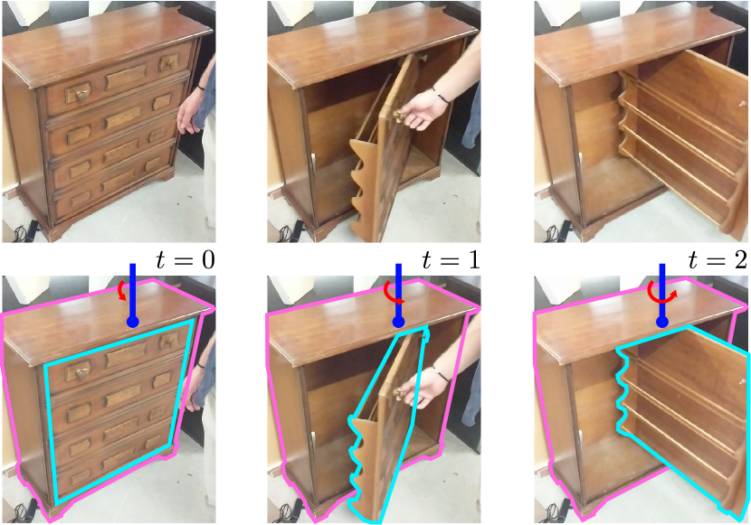
Figure 1: Object articulations often contradict categorical priors. While one would typically expect this drawer to contain prismatic joints, it actually has a single revolute joint. Our system is category-independent, predicting part poses (pink, cyan), joint parameters (blue), and time-varying configurations (red) from RGB-D sequences without category bias.

We propose a two-step approach to estimate articulation models, consisting of time-invariant joint parameters and time-varying joint states. Our method comprises a category-independent visual perception module for tracking part poses and a factor graph that estimates the articulation model governing part movements. First, we introduce a part pose tracking module that takes a sequence of RGB-D images of an object in motion as input and predicts part poses at every timestep. Second, we formalize articulation model estimation with a novel, factor graph-based structure. Notably, this two-step approach predicts articulation models without a category bias, thus providing generalization to novel instances without the need to first label them with the correct category. This is accomplished by first predicting and tracking part poses with learned motion features that we show are abstract enough to generalize to categories not seen during training, and second, by formulating the joint as a twist, which, compared to prior work [1, 2, 3, 4, 5, 6, 7, 8, 9, 10, 11], unifies the representation of prismatic, revolute, and helical joints. Fig. 1 highlights the need for category-independent articulation model prediction.

Finally, we propose a manipulation-oriented tangent similarity metric for evaluating articulation model estimates. Prior works evaluate the accuracy of the predicted joint types and axes [3, 6]. However, these metrics do not reflect how successful a robot might be at manipulating the articulated object given the predicted articulation model. Compliant controllers need to know the tangent direction in which to apply a force at a given time step, not necessarily whether the joint is prismatic or revolute [12, 13]. To that end, our proposed tangent similarity metric measures how accurately an estimated articulation model can predict the tangent direction for manipulation.

Using this metric, we first test the factor graph’s ability to predict articulation models from noisy pose observations and show that is more robust than a well-known baseline [3]. Second, we show that our full tracking and estimation pipeline outperforms another category-independent method [14].

II Related Work

II-1 Prior Object Knowledge

Existing estimation methods can be categorized into three groups based on the scope of tracked objects they can handle. Instance-level methods only estimate joint configurations for known or previously seen object instances [1, 7, 10]. Increasing in difficulty, category-level methods can handle unseen instances within a known category [8, 6, 15]. Finally, category-independent methods estimate joint mechanisms without any category information [14, 9, 16, 4, 2, 3, 11, 17, 5, 18, 19, 20]. In this paper, we propose a novel category-independent method, which assumes minimal prior knowledge about the object to avoid category bias.

II-2 Input Modality

Many works assume that a method to track part poses already exists and instead focus on articulation model estimation only, where the input is a sequence of 6D poses [3, 11, 4]. When used as a standalone module, the factor graph portion of our two-part pipeline can be seen as a member of this class.

Other works attempt to predict the articulation mechanism from a single observation, which could be an image [10, 7, 6, 1, 8, 9] or a (partial) point cloud [19, 20]. [21] propose a general object motion predictor for two consecutive RGB-D frames. Similarly, [18] use two point clouds with the object in two different states. However, it has been shown that an observation sequences can greatly improve estimates over time [3, 2].

To that end, many works track part poses from a sequence of images, either with a segmentation masks [14, 17, 9] or without [16, 5]. [15] track part poses from point cloud observations for known categories. [22] do not track over time but operate on the full set of point clouds and synchronize all of them.

Closest to our work, [2] tracks part poses from RGB-D images, but the image features they use require visually textured objects. While our part tracking module also tracks part poses from RGB-D images, we do not make assumptions about the visual appearance of objects.

II-3 Supported Joint Types

Commonly, it is assumed that parts are connected by a $1$-degree of freedom (DoF) joint—either a revolute hinge or a prismatic slider [1, 2, 3, 4, 5, 6, 7, 8, 9, 10, 11, 19]. Sturm et al. [3] are able to model joint types with up to five degrees of freedom by fitting a Gaussian process to part pose observations. In contrast to this non-parametric approach, [23] proposed a symbolic modeling language for arbitrary articulated objects.

In this work, we adopt and modify the screw representation of ScrewNet [14, 17]. While other approaches (e.g. [3, 2]) require different representations for prismatic/revolute joints and different logic to process each, the screw representation generalizes $1$-DoF prismatic, revolute, and helical joints into a single continuous representation.

II-4 Supported Kinematic Structures

While the joint type only models a local view of how two parts are connected, we are also interested in the overall kinematic structure of an object. The most general representation of this structure is through a graph, which allows arbitrarily connected parts [1, 2, 6, 10] and even closed-loop kinematic chains with interdependence between degrees of freedoms [3]. [4] propose configuration-dependent changes in a graph structure. Other works have simplified the general graph structure to a tree [5] or chain [16, 7], or abstained from considering the full kinematic structure by keeping to only local views of two parts [14, 17, 9, 11].

Our factor graph-based approach is inherently able to represent articulated objects with arbitrary kinematic structures. However, we restrict the experimental evaluation to articulated objects with a single prismatic or revolute joint.

II-5 Output Representation

The classical representation for articulation models is a joint axis paired with the joint type [3, 2, 10, 11, 7, 6, 8, 4, 1, 5, 9, 19]. Like [14, 17], we output joint twists instead, which avoids complications with optimizing over the hybrid continuous-discrete space of the classical representation. One might attempt to classify the joint type (prismatic vs. revolute) from the predicted twist. However, to successfully manipulate an articulated object, accurately predicting the ground truth joint type is unnecessary; compliant controllers can move articulated parts simply by applying the correct force in the object’s local frame [12, 11, 24]. Based on this idea, we formalize a new metric for evaluating articulated object models independent of their underlying ground truth kinematics.

III Background: Twist Joint Representation

We represent a motion constraint between two connected rigid bodies with joint parameters $\bm{\Theta}$ and time-varying joint configuration $\bm{q}$. The pose of the child body relative to its parent can be expressed as a function $f(\bm{q};\bm{\Theta})\in SE(3)$.

Specifically, in the case of helical joints, the joint parameters $\bm{\Theta}$ consists of the twist $\bm{\nu}=(\bm{v},\bm{\omega})\in se(3)$, where $\bm{v},\bm{\omega}\in\mathbb{R}^{3}$ describe the linear and angular motion, respectively. $se(3)$ is the Lie algebra of $SE(3)$. The joint configuration can be specified as a single scalar $q\in\mathbb{R}$. The helical joint function is defined as

$$f_{\text{twist}}\left(q;\bm{\nu}\right) =\operatorname{Exp}\left({q\bm{\nu}}\right)\in SE(3),$$ (1)

where $\operatorname{Exp}$ is the Lie exponential map.

Prismatic and revolute joints are special cases of helical joints, where $\bm{\omega}=\bm{0}$ for prismatic joints and $\bm{v}\times\bm{\omega}=\bm{0}$ for revolute joints.

IV Category-Independent Part Pose Tracking

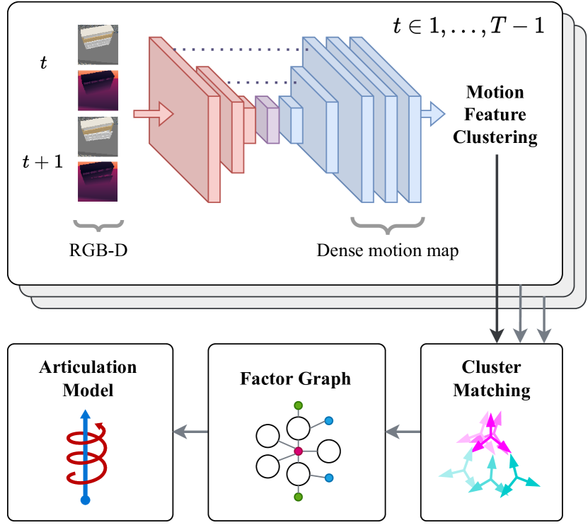
Figure 2: Full articulation model estimation pipeline. To detect and track part poses from RGB-D images, we first feed a pair of images from consecutive time steps to a motion feature predictor. This predictor outputs a pixel-level motion map that represents the center and delta pose of the part in each pixel. The motion map is then segmented into clusters, where the pixels in each cluster are aggregated to output the center and delta pose of a distinct part at the current time step. Detected parts are matched between time steps to form connected trajectories. The factor graph takes these predicted part trajectories and estimates the articulation model.

Our method is a two-step pipeline, shown in Fig. 2, comprised of a category-independent part pose tracking module and a factor graph-based articulation estimation module. The part pose tracking module, described in this section, detects and tracks poses of an articulated object’s parts from RGB-D images without any prior knowledge about the object’s category. The factor graph estimation module, described in Sec. V, takes in these part trajectories to estimate the articulation model.

The part pose tracking module takes in $T$ consecutive RGB-D images of a scene with one articulated object and outputs $T$ poses (part center and delta pose) for each part. We do not assume that the object or parts are segmented. The poses are represented in the camera frame.

The tracking is broken down into three steps: 1) a feature predictor encodes a pair of consecutive RGB-D images into a dense motion map, 2) the dense motion map is segmented into clusters representing detected parts, where the mean of the features within a cluster represents the predicted motion for the corresponding part at the current time step, and 3) the detected parts for the current time step are matched and appended to trajectory predictions from previous time steps. The sub-sections below describe each of these steps in detail.

IV-A Motion Feature Prediction

Inspired by [21], the motion feature predictor takes as input a pair of 6-channel RGB-XYZ images at time steps $t$ and $t+1$. The XYZ channels represent the $xyz$-coordinates of pixels in the camera frame, computed from the depth image. A ResNet-18 [25] encoder takes the pair of images and outputs a low-dimensional feature map for each. The feature maps are then fused with upconvolutions with skip connections to generate a single dense motion map. This map has ten channels and holds a prediction of the following quantities for each of $n\in\{1,\dots,\text{width}\times\text{height}\}$ pixels:

Importance $\beta_{n}^{(t)}\in\left[0,1\right]$ defined by the negative exponential distance to the image projected part center. Geometric part center $\bm{c_{n}}^{(t)}\in\mathbb{R}^{3}$ in the camera frame. Delta pose $\bm{\delta_{n}}^{(t)}\in se(3)$ of the part center from $t$ to $t+1$, represented in the camera frame. While [21] predicts a translation in camera frame, the rotation is predicted in an object-centric frame. Compared to that, we predict the rotation also in the camera frame, allowing us to use the full delta pose for predicting the part center at the next time step $\bm{\tilde{c}_{n}}^{(t+1)}=\operatorname{Exp}(\bm{\delta_{n}}^{(t)})\,\bm{c_{n}}^{(t)}$.

The training loss is computed for each pixel as the sum:

$$\mathcal{L} =\mathcal{L}_{\beta}+\beta(\gamma_{c}\mathcal{L}_{c}+\gamma_{\delta_{v}}\mathcal{L}_{\delta_{v}}+\gamma_{\delta_{\omega}}\mathcal{L}_{\delta_{\omega}}+\gamma_{\tilde{c}}\mathcal{L}_{\tilde{c}}$$

$$\hskip 47.0pt+\gamma_{\sigma_{c}}\mathcal{L}_{\sigma_{c}}+\gamma_{\sigma_{\delta}}\mathcal{L}_{\sigma_{\delta}}).$$ (2)

$\mathcal{L}_{\beta}$, $\mathcal{L}_{c}$, $\mathcal{L}_{\delta_{v}}$, $\mathcal{L}_{\delta_{\omega}}$, and $\mathcal{L}_{\tilde{c}}$ are squared L2 losses on the error between the motion feature predictions and their ground truth values ($\bm{\delta_{v}}$ and $\bm{\delta_{\omega}}$ are the linear and angular components of $\bm{\delta}$, respectively). $\mathcal{L}_{\sigma_{c}}$ and $\mathcal{L}_{\sigma_{\delta}}$ are unsupervised losses on the squared L2 norm of the variances of $\bm{c}$ and $\bm{\delta}$, respectively. For each pixel, the variance is computed with neighboring features within a $3\times 3$ window. These terms are designed to ensure the feature predictions are spatially consistent.

The $\gamma$ parameters can be tuned to scale the loss terms; for our experiments, we set $\gamma_{\delta_{\omega}}=10$ and the rest to $1$. All the terms except $\mathcal{L}_{\beta}$ are scaled by the importance parameter $\beta$ to prevent unimportant pixels from influencing the loss.

IV-B Motion Feature Clustering

Because object parts are rigid, pixels belonging to the same part should output similar centers and delta poses. This step therefore clusters together pixels in the feature map that belong to the same part. First, we filter out unimportant pixels by selecting the $N$ pixels with the highest importance $\beta_{n}^{(t)}$. On this subset, we perform spectral clustering, inspired by [22]. We construct an affinity matrix $\bm{A}^{(t)}\in\mathbb{R}^{N\times N}$

$$A_{ij}^{(t)}= \exp\frac{\|\bm{c_{i}}^{(t)}-\bm{c_{j}}^{(t)}\|^{2}}{-2\sigma_{A}^{2}}+\exp\frac{\|\bm{\tilde{c}_{i}}^{(t+1)}-\bm{\tilde{c}_{j}}^{(t+1)}\|^{2}}{-2\sigma_{A}^{2}},$$ (3)

where $i,j\in N$. $\sigma_{A}$ is a hyperparameter that controls how close centers should be to be considered part of the same cluster. We set $\sigma_{A}=0.05$\mathrm{m}$$.

We compute the singular value decomposition $\bm{U}\bm{\Sigma}\bm{V}^{T}=\bm{A}$ with singular values $\sigma_{1},\dots\sigma_{N}$ in descending order. The number of “significant” singular values are used to determine the number of clusters (i.e. parts) $K$. In other words, we want to find $K$ such that for all $i<K$, $\sigma_{i}\gg\sigma_{K}$. We determine $K$ by counting the singular values that are bigger than a fraction $\alpha$ of the sum of the first $M$ singular values:

$$K =\left|\left\{\sigma_{i}\mid\sigma_{i}\in\{\sigma_{1},\dots,\sigma_{N}\},\,\sigma_{i}>\alpha\sum\nolimits_{m=1}^{M}\sigma_{m}\right\}\right|$$ (4)

$M$ is a hyperparameter which determines the maximum number of parts an object can have; we set $M=9$ as a reasonably high value, considering the maximum number of parts in our experiments is actually $2$. While [22] uses a fixed $\alpha$ tuned specifically for the problem, we find this threshold dynamically at test time by building a histogram of $K$ computed over $100$ samples of $\alpha$ and choosing the most frequently occurring value of $K$.

Given $K$, we then perform $k$-means clustering on $\bm{U}$ with $K$ clusters, resulting in a set of pixels $N_{k}$ for each cluster $k\in K$. As each cluster represents a part, we compute the center and transformation for each part $k$ as an importance-weighted average over the pixels belonging to its cluster:

$$\bm{c_{k}}=\dfrac{\sum_{n\in N_{k}}\beta_{n}\bm{c_{n}}}{\sum_{n\in N_{k}}\beta_{n}},\qquad\bm{\delta_{k}}=\dfrac{\sum_{n\in N_{k}}\beta_{n}\bm{\delta_{n}}}{\sum_{n\in N_{k}}\beta_{n}},$$ (5)

where $N_{k}$ is the subset of $N$ pixels assigned to the $k$-th part.

IV-C Cluster Matching

The clusters are predicted from a pair of consecutive time steps, so they may not be temporally consistent over multiple time steps. The last step is to match clusters across time steps to turn motion features into a connected trajectory. We define a trajectory for part $k$ as a tuple $\xi_{k}=(C_{k},\Delta_{k})$, where $C=[\bm{c}^{(1)},\dots,\bm{c}^{(T)}]$ is the sequence of part centers and $\Delta=[\bm{\delta}^{(1)},\dots,\bm{\delta}^{(T)}]$ is the sequence of delta poses. The number of detected parts $K$ may change with each time step, so we keep a running list $\Xi=[\xi_{1},\dots,\xi_{L}]$ of trajectories for all the $L$ parts ever detected.

For each incoming detection result $(\bm{c_{k}}^{(t)},\bm{\delta_{k}}^{(t)})$ at time step $t$, we match the detection results to a trajectory $\xi_{l}\in\Xi$ by finding the one whose predicted center $\bm{\tilde{c}_{l}}^{(t)}=\operatorname{Exp}(\bm{\delta_{l}}^{(t-1)})~{}\bm{c_{l}}^{(t-1)}$ is closest to the incoming one:

$$l_{k} =\operatorname*{arg\,min}\nolimits_{l=1}^{L}\left\|\bm{\tilde{c}_{l}}^{(t)}-\bm{c_{k}}^{(t)}\right\|.$$ (6)

If the number of detected parts $K$ is greater than the number of trajectories $L$ in $\Xi$, then for every unassigned part $k$, we assume it did not previously move and create a new trajectory $\xi_{k}=([\bm{c_{k}}^{(t)},\dots,\bm{c_{k}}^{(t)}],[\bm{0},\dots,\bm{0},\bm{\delta_{k}}^{(t)}])$ of length $t$. If a previously detected part $l$ is not detected at $t$, then we assume the part did not move and append $(\bm{c_{l}}^{(t-1)},\bm{0})$ to $\xi_{l}$.

For selecting the part trajectories in $\Xi$ to use in downstream articulation model estimation, we assume that the articulated body has a single joint with one fixed and one moving part. The fixed base part is assigned to the trajectory with the lowest variance, and the moving part is assigned to the one with the fewest missing detections across all the time steps. This logic can be easily extended to longer kinematic chains by selecting more trajectories in order of detection reliability.

V Articulation Model Estimation

After detecting and tracking trajectories of part poses (e.g., with our visual perception module), the next step is to estimate the articulation model from the predicted part poses. We model this task as maximum a posteriori (MAP) estimation on a factor graph, an approach that has been shown to be extremely flexible for a range of estimation tasks in robotics [26, 27].

V-A Factor Graph Background

A factor graph is a bipartite graph that factorizes a probability distribution into conditionally-independent densities. We define each factor graph using a set of latent variables $\bm{X}$, a set of observed variables $\bm{O}$ and a set of factors $\bm{\phi}$. All factors $i$ follow the same structure of

$$\phi_{i}\left(\bm{X}_{i};\bm{O}_{i}\right)=\exp\left(-\frac{1}{2}\|\bm{r}_{i}\left(\bm{X}_{i};\bm{O}_{i}\right)\|_{\Sigma_{i}}\right)$$ (7)

where $\bm{X}_{i}\subseteq\bm{X}$ and $\bm{O}_{i}\subseteq\bm{O}$ are defined by the connectivity of the graph. $\|\bm{r}_{i}\left(\bm{X}_{i};\bm{O}_{i}\right)\|_{\Sigma_{i}}$ is the Mahalanobis distance $d_{i}$ with covariance matrix $\Sigma_{i}$ of a residual function $\bm{r}_{i}(\bullet)$. If a factor $\phi_{i}$ does not use any observations, $\bm{O}_{i}$ will be the empty set $\emptyset$ and for clarity we will drop $\bm{O}_{i}$ from the parameter list.

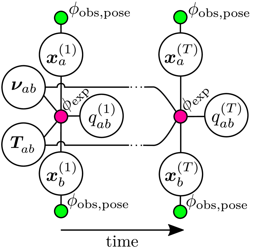
((a)) Pose observations

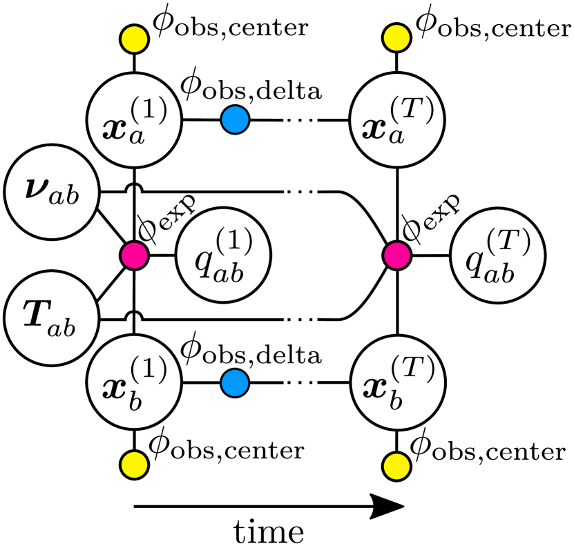
((b)) Center/delta pose observations

Figure 3: Our two factor graphs with different observation inputs, indicated by $\phi_{obs,\bullet}$ factors. Both factor graphs infer the same latent variables (white nodes). The exponential factor $\phi_{exp}$ connects the time-varying latent variables $\bm{x}^{(t)}$ and $q^{(t)}$ to the joint parameters $\bm{\nu}$ and $\bm{T_{ab}}$.

To improve convergence characteristics, we perform MAP estimation over the distribution specified by the factor graph using the Levenberg-Marquardt algorithm [28, Sec.4.7.3] on $P$ parallel, randomly initialized instances of the problem, and then select the solution with the lowest cost. For all of our experiments, we use $P=10$. For robustness against outliers, we use a Huber loss wrapped around the Mahalanobis distance $d_{i}$ of each factor with a small $\delta=0.01$:

$$L_{\delta}(d_{i})=\begin{cases}\frac{1}{2}{d_{i}^{2}}&\text{for }|d_{i}|\leq\delta,\\ \delta(|d_{i}|-\frac{1}{2}\delta),&\text{otherwise.}\end{cases}$$ (8)

V-B Proposed Factor Graph

In Fig. 3, we propose two factor graphs, which share the same latent structure but have different observations attached. We will now first explain the shared latent structure and then how the different observations are incorporated.

Both factor graphs contain latent part poses $\tensor[]{\bm{x}}{}_{k}^{(t)}$, one pose per detected part $k\in\left[1,K\right]$ at each time step $t\in\left[1,T\right]$. For each pair of parts $(a,b)$ that are connected through a joint, we aim to estimate a sequence of time-varying joint configurations $q_{ab}^{(t)}$ and a pair of time-invariant joint parameters $(\bm{\nu_{ab}},\bm{T_{ab}})$.

Similarly to [14], we parameterize the joint with a twist $\bm{\nu}=(\bm{v},\bm{\omega})$ that is able to express rigid, prismatic, revolute and helical joint types. However, while [14] uses two scalar parameters to scale $\bm{v}$ and $\bm{\omega}$ separately, we use a single joint configuration parameter $q^{(t)}\in\mathbb{R}$ to scale the entire twist, as described in Eq. 1.

To allow arbitrary local frame placements for the articulated parts, we incorporate an additional transformation $\tensor[]{\bm{T}}{{}_{\text{twist}}}\in SE(3)$ from the twist frame to the camera frame, as done in [3]. The joint articulation function then becomes:

$$f_{\text{twist}}\left(q^{(t)};\bm{\nu},\tensor[]{\bm{T}}{{}_{\text{twist}}}\right)=\tensor[]{\bm{T}}{{}_{\text{twist}}}\operatorname{Exp}\left({q^{(t)}\bm{\nu}}\right).$$ (9)

At each time step, the joint variables and latent poses are connected through the exponential factor $\phi_{exp}$. This factor compares the relative transformation between the latent part poses $\left(\tensor[]{\bm{x}}{{}_{a}}\right)^{-1}\tensor[]{\bm{x}}{{}_{b}}$ to the expected transformation computed by the joint function $f_{\text{twist}}(q_{ab};\bm{\nu_{ab}},\bm{T_{ab}})$. The residual error is computed by:

$$\bm{r}_{\text{exp}}\left(\bm{X}_{\text{exp}}=\left\{\bm{x_{a}},\bm{x_{b}},\bm{T_{ab}},\bm{\nu_{ab}},q_{ab}\right\}\right)$$

$$\quad=f_{\text{twist}}(q_{ab};\bm{\nu_{ab}},\bm{T_{ab}})\ominus(\bm{x_{a}}^{-1}\bm{x_{b}}),$$ (10)

where $\ominus$ is the twist error between two poses $\bm{x},\bm{y}\in SE(3)$:

$$\bm{x}\ominus\bm{y} =\operatorname{Log}(\bm{x}^{-1}\bm{y})\in se(3).$$ (11)

The factor graph can infer its latent variables from different observations, depending on what the upstream perception method predicts. Thus, the factor graph could be used in conjunction with a wide range of perception methods. In the following, we highlight three possible observation types: pose observations (e.g., from CAPTRA [15]), centers, and pose changes (e.g., from our proposed part tracking method).

V-B1 Part Pose Observation

If the perception method tracks full 6D poses for each articulated body part, we can use the observation factor $\phi_{\text{obs},\text{pose}}$ to compare an observed pose $\tensor[]{\bm{y}}{}\in SE(3)$ to a latent pose $\tensor[]{\bm{x}}{}$ with the residual

$$\bm{r}_{\text{obs},\text{pose}}\left(\bm{X}_{\text{obs},\text{pose}}=\left\{\tensor[]{\bm{x}}{}\right\};\bm{O}_{\text{obs},\text{pose}}=\left\{\tensor[]{\bm{y}}{}\right\}\right)$$

$$\quad=\tensor[]{\bm{x}}{}\ominus\tensor[]{\bm{y}}{}.$$ (12)

V-B2 Part Center Observation

If the perception method only tracks the positions of part centers, we use the part center observation factor $\phi_{\text{obs},\text{center}}$ to compare the observed part center $\bm{c}$ to the position portion of the latent part pose $\tensor[]{\bm{x}}{}_{p}$ with the residual

$$\bm{r}_{\text{obs},\text{center}}\left(\bm{X}_{\text{obs},\text{pose}}=\left\{\tensor[]{\bm{x}}{}\right\};\bm{O}_{\text{obs},\text{center}}=\left\{\bm{c}\right\}\right)$$

$$\quad=\tensor[]{\bm{x}}{}_{p}-\bm{c}.$$ (13)

V-B3 Part Pose Change Observation

If the perception method tracks the changes in part poses between consecutive time steps, we use the delta pose observation factor $\phi_{\text{obs},\text{delta}}$ to compare the observed delta pose $\bm{\delta}^{(t)}\in se(3)$ expressed in the world frame with the latent poses $\tensor[]{\bm{x}}{}^{(t)}$ and $\tensor[]{\bm{x}}{}^{(t+1)}$:

$$\bm{r}_{\text{obs},\text{delta}}\left(\bm{X}_{\text{obs},\text{delta}}=\left\{\tensor[]{\bm{x}}{}^{(t)},\tensor[]{\bm{x}}{}^{(t+1)}\right\};\bm{O}_{\text{obs},\text{delta}}=\left\{\bm{\delta}^{(t)}\right\}\right)$$

$$\quad=\left(\operatorname{Exp}(\bm{\delta}^{(t)})~{}\tensor[]{\bm{x}}{}^{(t)}\right)\ominus\tensor[]{\bm{x}}{}^{(t+1)}.$$ (14)

VI Tangent Similarity Metric

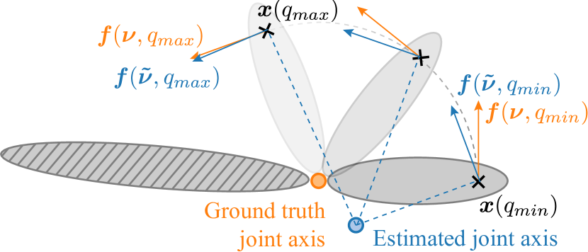
Figure 4: The tangent similarity metric measures the cosine similarity between the predicted linear velocity $\bm{f}(\bm{\tilde{\nu}},q)$ and ground truth $\bm{f}(\bm{\nu},q)$ along the path traced by the grasping point $\bm{x}(q)$.

We introduce a new error metric for articulation models that captures how useful a prediction is for robot manipulation. A commonly used metric is the angle error of the predicted joint axis. However, when the joint type is unknown, this metric can be misleading; the predicted joint axis could have 0 angle error, but if the predicted joint type (i.e. prismatic vs. revolute) is wrong, the predicted axis actually captures an orthogonal range of motion and thus is useless for manipulation. Meanwhile, a prediction with the incorrect joint type and axis may actually be sufficient to manipulate the object if the tangent direction points in the correct direction. Our ultimate goal is to manipulate articulated objects, so we propose a metric that measures how well a robot would be able to manipulate the articulated object given an estimated articulation model.

More formally, suppose we have two rigid bodies connected by a single twist joint parameterized by $\bm{\nu}=(\bm{v},\bm{\omega})\in se(3)$. We assume one body is a rigid base, and we want to manipulate the second body by grasping it at a given fixed point and pulling it such that the joint configuration $q$ goes from $q_{min}$ to $q_{max}$. Let $\bm{x_{0}}$ be the grasping point when $q=0$. The grasping point follows the path

$$\bm{x}(q) =\operatorname{Exp}\left({q\bm{\nu}}\right)\bm{x_{0}}\in\mathbb{R}^{3}$$ (15)

for the range $q\in[q_{min},q_{max}]$. A visualization is presented in Fig. 4.

At test time, the joint motion is unknown, so we need to predict it. Let $\bm{\tilde{\nu}}=(\bm{\tilde{v}},\bm{\tilde{\omega}})\in se(3)$ be a prediction of the joint motion. We assume that we want to manipulate the articulated body using the predicted joint motion with a rigid grasp at the grasping point.

We define the tangent similarity metric as the average cosine similarity between the predicted and true linear velocities $\bm{\tilde{v}}$ and $\bm{v}$ at the grasping point along the path $\bm{x}(q)$:

$$J(\bm{\nu},\bm{\tilde{\nu}}) =\frac{1}{q_{max}-q_{min}}\int_{q_{min}}^{q_{max}}\frac{\bm{f}(\bm{\nu},q)}{\|\bm{f}(\bm{\nu},q)\|}\cdot\frac{\bm{f}(\bm{\tilde{\nu}},q)}{\|\bm{f}(\bm{\tilde{\nu}},q)\|}~{}dq$$

where

$$\bm{f}(\bm{\nu},q) =\bm{Ad}_{\operatorname{Exp}\left({\bm{x}(q)}\right)^{-1}}(\bm{\nu})_{\bm{v}}$$ (16)

$$=\bm{v}+[\bm{\omega}]_{\times}\bm{x}(q).$$

The adjoint operator $\bm{Ad}_{\operatorname{Exp}\left({\bm{x}(q)}\right)^{-1}}:se(3)\rightarrow se(3)$ takes the twist $\bm{\nu}$ and transforms it to the local frame of the grasping point $\bm{x}(q)\in\mathbb{R}^{3}$ via the transformation $\operatorname{Exp}\left({\bm{x}(q)}\right)^{-1}\in SE(3)$. For this metric, we are only concerned with the linear component $\bm{\nu}_{\bm{v}}$ of the resulting twist. A perfect prediction yields $1$, while an orthogonal prediction yields $0$.

While the integral does not have a closed form solution, we can easily approximate it with equally spaced samples of $q$ in the range $[q_{min},q_{max}]$; for the joint ranges used in our experiments, we found $100$ samples was enough to accurately estimate within $\pm 0.001$.

This metric is physically meaningful, since it measures how much of an applied force would be able to move the second body in the direction of joint motion. If a force that is constantly $60^{\circ}$ off is applied to the second body, $\cos(60^{\circ})=0.5$. Therefore, half of the applied force would still be in the direction of joint motion and this metric would yield $0.5$. In other words, this component of the applied force could move the second body with half the effectiveness.

VII Experiments

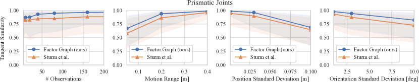
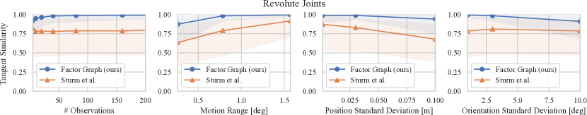
Figure 5: Comparison between articulation model estimation methods (FG, Sturm) on synthetically generated noisy data. The lines represent the median tangent similarity score (1.0 represents a perfect prediction) over 50 runs, while the shaded region represents the 25th and 75th percentiles. The first two columns show that both methods benefit from an increased number of observations and larger motion ranges, but FG is able to achieve nearly perfect scores with fewer observations and smaller motion ranges. The last two columns show that FG is more robust to position and orientation noise.

In the experiments, we test two hypotheses. H1: The factor graph is able to outperform baselines as a standalone articulation module estimation module when given noisy pose data. H2: Explicitly tracking part poses allows the full tracking and estimation pipeline to generalize across object categories.

VII-A Factor Graph Experiment (H1)

In this experiment, we evaluate the factor graph’s ability to handle noisy pose observations. The factor graph (FG) can be used as a standalone module that estimates articulation models from part poses, just like Sturm et al. [3] (Sturm). Therefore, we use Sturm as a baseline evaluating on two types of pose data: 1) synthetically generated data with controlled noise and 2) predicted poses from a state-of-the-art category-level part tracking method, CAPTRA [15]. Since CAPTRA assumes that the joint type is already known, the role of FG and Sturm when used in conjunction with CAPTRA is to solely estimate the joint parameters for the known joint type. The purpose of this experiment is to show how the methods handle predictions from a learned system with non-Gaussian noise characteristics.

VII-A1 Setup

Variable	Values
# observations $T$	$\{5,10,20,40,80,160,320\}$
Motion range $q_{\max}$	$\begin{array}[]{rl}\text{revolute:}&\{15\degree,45\degree,90\degree\}\\ \text{prismatic:}&\{0.05$\mathrm{m}$,0.2$\mathrm{m}$,0.4$\mathrm{m}$\}\\ \end{array}$
Position noise $\sigma_{\text{pos}}$	$\{0.001$\mathrm{m}$,0.03$\mathrm{m}$,0.1$\mathrm{m}$\}$
Orientation noise $\sigma_{\text{ori}}$	$\{1.0\degree,3.0\degree,10.0\degree\}$

TABLE I: Parameters used for the synthetic pose experiment.

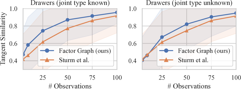
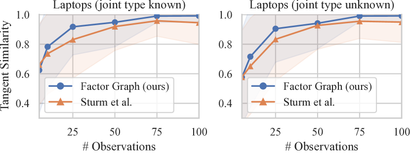
Figure 6: Articulation model estimation using part poses provided by CAPTRA. Since CAPTRA assumes the joint type is known, we test FG and Sturm with and without the known joint type constraints. We plot the mean and standard deviation tangent similarity scores over 60 simulation runs.

For Sturm, we use the original implementation of Sturm et al. [3] with its provided parameters. During initial testing, Sturm sometimes misclassified joints as rigid; since the joints are always either prismatic or revolute in our experiments, we removed rigid joints from Sturm for a fair comparison. Sturm takes $6$-DoF part poses as input, so we use FG with pose observation factors (Fig. 3(a)). We set the noise parameters for both FG and Sturm to the same noise parameters used to generate the synthetic and CAPTRA data.

To generate synthetic pose data, we vary four parameters: the number of observations, the range of the articulated motion, the position noise, and the orientation noise. The exact parameter values are given in Table I. Details on how the noisy poses are generated are included in Appx. B-A.

For CAPTRA data, we use 60 simulation runs each for two categories, Drawer and Laptop, from the simulated SAPIEN dataset [15] on which CAPTRA was tested.

Since CAPTRA assumes that the joint type is known, we also evaluate FG and Sturm with the joint type given. For FG, this means adding a constraint to ensure that the predicted twist $\bm{\nu}=(\bm{v},\bm{\omega})$ obeys the given joint constraint: $\bm{\omega}=\bm{0}$ for prismatic joints and $\bm{v}\times\bm{\omega}=\bm{0}$ for revolute joints.

VII-A2 Results

The results for the synthetic pose experiment are shown in Fig. 5. FG outperforms Sturm for both joint types, but especially for revolute joints. Sturm performs worse with revolute joints because it has a tendency to misclassify revolute joints as prismatic.

The results for the CAPTRA pose experiment are shown in Fig. 6. FG performs better than Sturm for the Laptop category, and achieves high scores with fewer observations (i.e. better sample efficiency) for the Drawer category. Sturm did not benefit from knowing the joint type, while FG did; this information helped improve its sample efficiency for the Drawer category. Both methods performed worse for drawers than laptops, likely due to the fact that CAPTRA prediction errors were larger for Drawer parts ($0.465$\mathrm{c}\mathrm{m}$$) than for Laptop parts ($0.335$\mathrm{c}\mathrm{m}$$).

Fig. 7 shows qualitative real world results using CAPTRA to track part poses of a drawer.

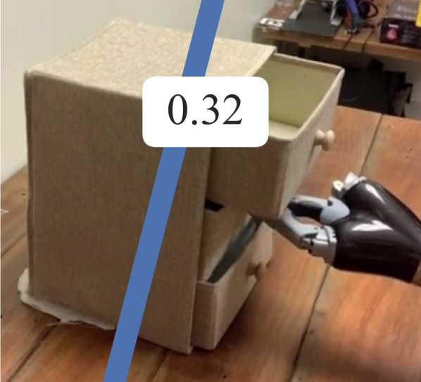
((a)) $t=0$\mathrm{s}$$

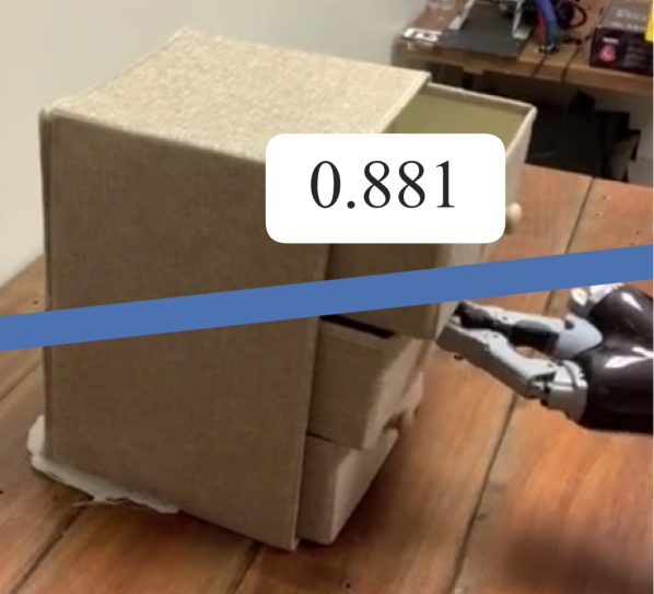
((b)) $t=1$\mathrm{s}$$

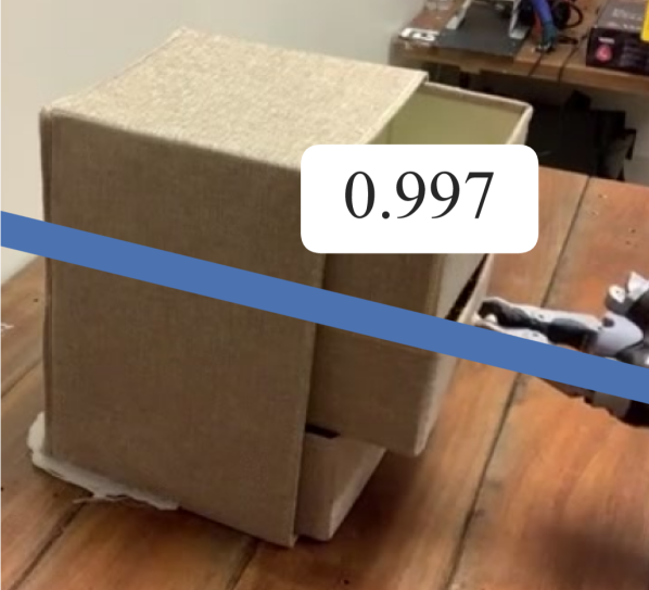
((c)) $t=2$\mathrm{s}$$

Figure 7: Real world results using CAPTRA for part pose tracking and FG for articulation model estimation. The blue line shows the estimated joint axis. As the robot interacts with the object, the estimate becomes more accurate, as indicated by the tangent similarity score shown in the white box.

VII-B Full Pipeline Experiment (H2)

Method		Prior Visual Information
Visual Perception	Estimation
Ours (PT)	Factor Graph (FG)	None
Ours (PT)	Sturm et al. [3] (Sturm)	None
ScrewNet [14] (ScrewNet)		Two parts segmented

TABLE II: Overview of the three methods we evaluate in the full pipeline experiment. ScrewNet [14] is an end-to-end method that handles both visual perception and estimation but requires part segmentations as input.

In this experiment, we evaluate the category-independent part pose tracking module (PT) proposed in Sec. IV used in conjunction with the factor graph (PT+FG) against two baselines: PT with Sturm et al. [3] (PT+Sturm) and ScrewNet [14] (see Table II).

VII-B1 Setup

We use simulated data generated from the PartNet-Mobility dataset [29]. Since ScrewNet requires object part segmentations, we provide ground truth segmentations from the simulation. The segmentations are not given to PT+FG or PT+Sturm, since our part tracking module can detect and track object parts without segmentations.

We also modified ScrewNet to predict the twist in the camera frame rather than an object-centric frame (like [17]). Additionally, we evaluate ScrewNet’s predictions using our metric introduced in Sec. VI. For further details see Appx. A.

We conduct three category-independent experiments: 1) train and test on prismatic objects (Prismatic), 2) train and test on revolute objects (Revolute), and 3) train and test on both prismatic and revolute objects (Mixed). To evaluate ability of the methods to generalize across categories, the test sets include only objects from categories not present in the training set (Refrigerator and Table). For further details, see Appx. B-B.

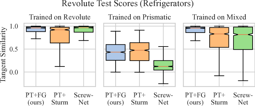
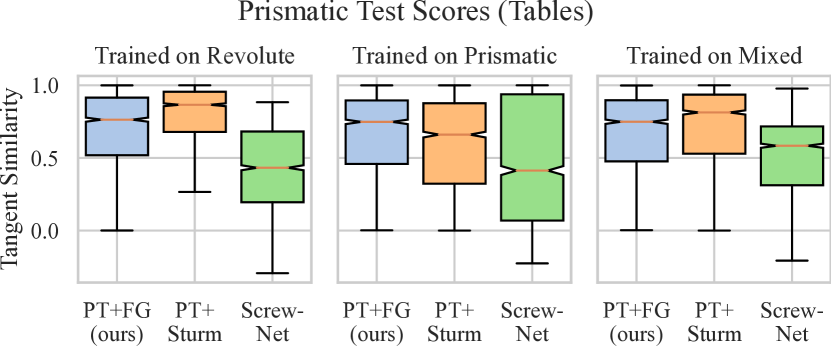
Figure 8: Comparison between part tracking+estimation methods (PT+FG, PT+Sturm, ScrewNet) on RGB-D data from PartNet-Mobility. To test category independence, models are trained on Prismatic, Revolute, and Mixed objects, and then evaluated on unseen categories (Refrigerator and Table). Our method (PT+FG) nearly matches or outperforms the baselines in all train/test combinations.

VII-B2 Results

Results for the full pipeline experiment on simulated data are shown in Fig. 8. Our approach (PT+FG) shows the most consistent result across all experiments, while PT+Sturm and ScrewNet are more sensitive to the underlying training data. This demonstrates two points. First, the fact that the underlying training distributions do not matter as much for (PT+FG) indicates that PT is able to learn the concept of articulated part motion on a pixel-level. Second, PT is robust to imbalances in the training set.

Qualitative results are discussed in Fig. 9.

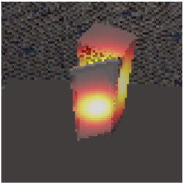
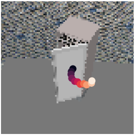
Figure 9: Visualization of our full tracking and estimation pipeline (PT+FG) on a object from the Refrigerator category of the PartNet-Mobility data set. The left image shows the importance predictions output by PT; it learns to focus on the centers of the two cabinet parts (without being given segmentation masks). The middle image shows the predicted part poses output by PT. The right image shows the tangent motion directions of the twist predicted by FG; this prediction achieves a nearly perfect tangent similarity score of 0.999.

VIII Conclusion

We present a full pipeline to track and estimate articulated objects on a stream of RGB-D images. We test our estimation method in isolation, outperforming a well established baseline, and show the applicability of our approach on real world data. Our full pipeline performs more consistently than previous category-independent methods without requiring object part segmentation masks. For evaluation, we propose a manipulation-oriented tangent similarity metric that allows a coherent comparison across different joint types.

Possible extensions of this work include applications to articulated objects with multiple joints or leveraging recent techniques for end-to-end optimization through probabilistic state estimators [27, 30, 31]. We also plan to extend the tangent similarity metric with a rotation component to capture manipulability for objects like knobs and screw caps.

Appendix A Tangent Similarity Metric for ScrewNet Predictions

For each timestep $t$, ScrewNet [14] outputs a tuple $\left(\bm{l},\bm{m},\theta,d\right)^{(t)}$ that represents the relative transformation between two parts. Here, $\bm{l}$ and $\bm{m}$ are the Plücker coordinates of the axis $l=\bm{p}+x\bm{l}$, where $\bm{m}=\bm{p}\times\bm{l}$ holds. $\theta$ is the rotation around and $d$ the displacement along the aforementioned axis [14]. The axis is defined in the camera frame.

As derived in [32], we compute the twist $\bm{\nu}^{(t)}=(\bm{v},\bm{\omega})\in se(3)$ that describes the relative motion of the body as

$$\bm{\nu}^{(t)}=\begin{bmatrix}\bm{v}\\ \bm{\omega}\end{bmatrix}=\begin{bmatrix}-\theta\bm{m}+d\bm{l}\\ \theta\bm{l}\end{bmatrix}$$ (17)

given the time-indexed ScrewNet outputs $\left(\bm{l},\bm{m},\theta,d\right)^{(t)}$.

As before, we are interested in the linear velocity along the grasp path. Due to ScrewNet’s time-varying predictions of joint twists $\bm{\nu}^{(t)}$, we need to replace the analytical model introduced in Sec. VI with a time-indexed approximation. The problem is framed as follows.

Given both the ground truth twist $\bm{\nu}^{(t)}$ and predicted twist $\tilde{\bm{\nu}}^{(t)}$ at time $t$, we want to compare their linear velocity at grasping point $\bm{x}(t)\in\mathbb{R}^{3}$. Similarly to Eq. 16, the linear velocity component at the grasping point is computed as

$$\bm{f}\left(\bm{x},\bm{\nu}\right) =\bm{\bm{Ad}}_{\operatorname{Exp}\left({\bm{x}}\right)^{-1}}(\bm{\nu})_{\bm{v}}$$ (18)

$$=\bm{v}+[\bm{\omega}]_{\times}\bm{x}.$$ (19)

The time-indexed similarity score then becomes

$$J\left(\bm{\nu}^{(1:T)},\tilde{\bm{\nu}}^{(1:T)}\left|\bm{x}^{(1:T)}\right.\right)$$

$$\quad=\frac{1}{T}\sum_{t}\frac{\bm{f}\left(\bm{x}^{(t)},\bm{\nu}^{(t)}\right)\cdot\bm{f}\left(\bm{x}^{(t)},\tilde{\bm{\nu}}^{(t)}\right)}{\|\bm{f}\left(\bm{x}^{(t)},\bm{\nu}^{(t)}\right)\|\|\bm{f}\left(\bm{x}^{(t)},\tilde{\bm{\nu}}^{(t)}\right)\|}.$$ (20)

Appendix B Experiment Data

B-A Factor Graph Experiment (H1)

B-A1 Synthetic Noisy Poses

The goal of this experiment is to create synthetic poses that resemble the most simple kinematic structures of real, articulated household objects that have a fixed base part and one moving articulated part. Initially, the fixed base part $\tensor[]{\bm{x}}{{}_{a}}^{(t)}\in SE(3)$ is given the same random orientations for all time steps $t\in\left[1,\ldots,T\right]$. Then, we sample a sequence of synthetic poses in the following manner.

First, we sample a random transformation from the first part $a$ to the joint frame $\tensor[^{a}]{\bm{T}}{{}_{j}}$. We uniformly sample an orientation in the full rotation space and a position between $-0.5$\mathrm{m}$$ and $0.5$\mathrm{m}$$. We sample an additional random transformation $\tensor[^{j}]{\bm{T}}{{}_{b}}$ from the joint to the second part $b$. The joint state is defined to be zero at the first time step, and thus part $b$ is placed at $\tensor[]{\bm{x}}{{}_{b}}^{(1)}=\tensor[]{\bm{x}}{{}_{a}}^{(t)}\tensor[^{a}]{\bm{T}}{{}_{j}}\tensor[^{j}]{\bm{T}}{{}_{b}}\in SE(3)$.

Next, we sample a random canonical twist $\bm{\nu}$ depending on the desired joint type, either prismatic or revolute. Based on that twist, we can then easily generate the full pose sequence for the second part. We denote $q_{\max}$ as the motion magnitude (i.e. how much the joint is actuated). The units of $q_{\max}$ are meters for prismatic joints and radians for revolute joints. We use the notation introduced Sec. III to represent the joint. We then define the poses for the second body as

$$\tensor[]{\bm{x}}{{}_{b}}^{(t)}=\tensor[]{\bm{x}}{{}_{a}}^{(t)}\tensor[^{a}]{\bm{T}}{{}_{j}}\operatorname{Exp}\left({\frac{t-1}{T-1}q_{\max}\bm{\nu}}\right)\tensor[^{j}]{\bm{T}}{{}_{b}}$$ (21)

for each time step $t=\left[1,\ldots,T\right]$.

Next, we shift the positions of both bodies such that the overall position mean is 0, centering the full, hypothetical object around the origin.

Lastly, we apply Gaussian noise to all poses to obtain noisy observations for our experiment. The noise is generated by first sampling perturbation twists from a Gaussian distribution

$$\bm{\nu}_{\text{perp}}\sim\mathcal{N}(0,\Sigma^{2})$$ (22)

where $\Sigma^{2}=\text{diag}\left(\sigma_{\text{pos}}^{2},\sigma_{\text{pos}}^{2},\sigma_{\text{pos}}^{2},\sigma_{\text{ori}}^{2},\sigma_{\text{ori}}^{2},\sigma_{\text{ori}}^{2}\right)$, where position and orientation noise parameters $\sigma_{\text{pos}}^{2},\sigma_{\text{pos}}^{2}$ are defined by the experiment. We apply the perturbation twist by multiplying by its exponentiation

$$\tensor[]{\bm{y}}{}=\tensor[]{\bm{x}}{}\operatorname{Exp}\left({\bm{\nu}_{\text{perp}}}\right).$$ (23)

B-B Full Pipeline Experiment (H2)

B-B1 Simulation

We use a PyBullet Simulation to generate training and test data. A single object from our object instance set (see below) is loaded and randomly translated and rotated around the z-axis before being placed onto a table. Additionally, for each simulation run we randomly sample a camera position and orientation facing the front of the object. We then render RGB-D images for 11 consecutive, different joint configurations. We start with the default joint configuration and randomly increase the joint configuration by a percentage of its max joint range. We randomly sample the percentage from a Gaussian with mean of $8\%$ and standard deviation of $2\%$. Upon reaching the joint limit, we switch the direction of joint motion and start decreasing the joint configuration.

B-B2 Object Set

For our experiments, we consider a set of household categories from the full PartNet-Mobility dataset [29], namely the categories: Box, Dishwasher, Door, Laptop, Microwave, Oven, Refrigerator, StorageFurniture, Table, WashingMachine, Window. Unlike previous work [14, 15], we do not manually select instances from the PartNet-Mobility dataset but rather automatically parse all object instances and then filter out instances that have more than one joint, have an unlimited joint range and/or have a joint range less than $10\degree$ or $0.1m$, respectively. An overview of our resulting training and test sets are given in Tab. III and Tab. IV.

Joint Type	Categories	Unique instances	Simulation Runs
Revolute	no Refrigerator	220	17516
Prismatic	no Table	18	9311
Mixed	no Refrigerator and no Table	$237^{*}$	$26748^{*}$

TABLE III: Overview of our three training datasets. As the amount of unique instances for the prismatic joint type is low compared to the revolute joint type, we purposely created more simulation runs for these object instances to better balance the data sets.
^∗The one instance and $79$ simulation runs discrepancy between the sum of the revolute set (first row) and the prismatic set (second row) to the mixed set (third row) is because the PartNet-Mobility dataset has one Table instance with a revolute joint. This instance was included in the revolute set (first row), and not included in the mixed set (third row).

Joint Type	Categories	Unique instances	Simulation Runs
Revolute	Fridges	14	1095
Prismatic	Tables	25	1951

TABLE IV: Overview of our test data sets.

B-B3 Category-Level Experiment

For completeness, we additionally perform a category-level experiment for our two previously held-out test categories, Table and Fridge. In a category-level experiment, all instances come from the same PartNet-Mobility category, but the training and test set do not share any instances. We split the Fridge instances into 10 training and 4 test instances, and the Table instances into 18 training and 7 test instances.

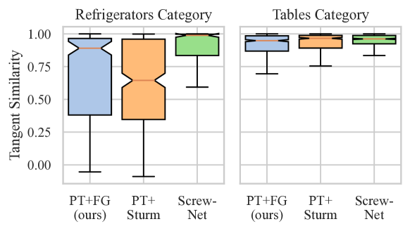
Figure 10: Category level experiment. The worse performance of our method on the Fridge category is due to observed overfitting of our motion feature predictor.

Results for this experiment are shown in Fig. 10. All methods perform well on the Table category but perform worse on the Fridge category. We suspect the main reason is that the Fridge category contains fewer training instances. Additionally, the revolute Fridge joint requires tracking the full 6D pose of the moving part, while the prismatic Table joint only requires tracking translation.

Comparing PT+FG and PT+Sturm to ScrewNet, it is visible that ScrewNet performs better. Compared to ScrewNet, our motion feature predictor outputs low-level motion features, for which the joint type does not matter. As mentioned in Appx. A, ScrewNet predicts the displacement along and rotation around a predicted axis. Therefore, if all object instances in the training data share the same joint type (i.e. are from the same category as in this experiment), either only the displacement or rotation will vary in the training data. Thus, ScrewNet is given an implicit bias, whereas PT predicts low-level geometric features and does not make use of that bias. Therefore, ScrewNet shows better performance in the cateogry-level experiment. Furthermore, this implicit bias can also explain the worse performance of ScrewNet for the category-independent experiment shown in Fig. 8, specifically the transfer between a model trained on Prismatic and tested on Revolute and vice versa. In this setup, the implicit bias hurts ScrewNet, since the training joint type is different from the test joint type, and PT+FG and PT+Sturm perform better.

Overall, these additional experiments further highlight that a more diverse data set helps for learning general low-level motion features that transfer well in a category-independent setting.

References

- [1] J. Pavlasek, S. Lewis, K. Desingh, and O. C. Jenkins, “Parts-based articulated object localization in clutter using belief propagation,” in IEEE/RSJ Int. Conf. on Intelligent Robots and Systems (IROS), 2020, pp. 10 595–10 602.
- [2] R. Martín-Martín and O. Brock, “Coupled recursive estimation for online interactive perception of articulated objects,” The Int. Journal of Robotics Research, 2019.
- [3] J. Sturm, C. Stachniss, and W. Burgard, “A probabilistic framework for learning kinematic models of articulated objects,” J. Artif. Intell. Res., vol. 41, pp. 477–526, 2011.
- [4] A. Jain and S. Niekum, “Learning hybrid object kinematics for efficient hierarchical planning under uncertainty,” in IEEE/RSJ Int. Conf. on Intelligent Robots and Systems (IROS), 2020, pp. 5253–5260.
- [5] A. F. Daniele, T. M. Howard, and M. R. Walter, “A multiview approach to learning articulated motion models,” in Int. Symp on Robotics Research (ISRR), 2017, pp. 371–386.
- [6] B. Abbatematteo, S. Tellex, and G. Konidaris, “Learning to generalize kinematic models to novel objects,” in Conf. on Robot Learning (CoRL), 2019, pp. 1289–1299.
- [7] F. Michel, A. Krull, E. Brachmann, M. Y. Yang, S. Gumhold, and C. Rother, “Pose estimation of kinematic chain instances via object coordinate regression,” in Proc. of the British Machine Vision Conf. BMVA Press, 2015, pp. 181.1–181.11.
- [8] X. Li, H. Wang, L. Yi, L. J. Guibas, A. L. Abbott, and S. Song, “Category-level articulated object pose estimation,” in IEEE/CVF Conf. on Computer Vision and Pattern Recognition (CVPR), 2020, pp. 3703–3712.
- [9] V. Zeng, T. E. Lee, J. Liang, and O. Kroemer, “Visual identification of articulated object parts,” in IEEE/RSJ Int. Conf. on Intelligent Robots and System (IROS), 2021, pp. 2443–2450.
- [10] S. Pillai, M. R. Walter, and S. J. Teller, “Learning articulated motions from visual demonstration,” in Robotics: Science and Systems (RSS), 2014.
- [11] K. Hausman, S. Niekum, S. Osentoski, and G. S. Sukhatme, “Active articulation model estimation through interactive perception,” in IEEE Int. Conf. on Robotics and Automation (ICRA), 2015, pp. 3305–3312.
- [12] M. Prats, P. J. Sanz, and A. P. del Pobil, “A framework for compliant physical interaction,” Auton. Robots, vol. 28, no. 1, pp. 89–111, 2010.
- [13] R. M. Martín and O. Brock, “Online interactive perception of articulated objects with multi-level recursive estimation based on task-specific priors,” in IEEE/RSJ Int. Conf. on Intelligent Robots and Systems (IROS), 2014, pp. 2494–2501.
- [14] A. Jain, R. Lioutikov, C. Chuck, and S. Niekum, “ScrewNet: Category-independent articulation model estimation from depth images using screw theory,” in IEEE Int. Conf. on Robotics and Automation (ICRA), 2021, pp. 13 670–13 677.
- [15] Y. Weng, H. Wang, Q. Zhou, Y. Qin, Y. Duan, Q. Fan, B. Chen, H. Su, and L. J. Guibas, “CAPTRA: category-level pose tracking for rigid and articulated objects from point clouds,” in IEEE/CVF Int. Conf. on Computer Vision (ICCV), 2021, pp. 13 189–13 198.
- [16] Q. Liu, W. Qiu, W. Wang, G. D. Hager, and A. L. Yuille, “Nothing but geometric constraints: A model-free method for articulated object pose estimation,” CoRR, vol. abs/2012.00088, 2020.
- [17] A. Jain, S. Giguere, R. Lioutikov, and S. Niekum, “Distributional depth-based estimation of object articulation models,” in Conf. on Robot Learning (CoRL), 2021, pp. 1611–1621.
- [18] L. Yi, H. Huang, D. Liu, E. Kalogerakis, H. Su, and L. J. Guibas, “Deep part induction from articulated object pairs,” ACM Trans. Graph., vol. 37, no. 6, p. 209, 2018.
- [19] Z. J. Yew and G. H. Lee, “Rpm-net: Robust point matching using learned features,” in IEEE/CVF Conf. on Computer Vision and Pattern Recognition, (CVPR), 2020, pp. 11 821–11 830.
- [20] X. Wang, B. Zhou, Y. Shi, X. Chen, Q. Zhao, and K. Xu, “Shape2Motion: Joint Analysis of Motion Parts and Attributes From 3D Shapes,” in IEEE/CVF Conf. on Computer Vision and Pattern Recognition (CVPR), Jun. 2019, pp. 8868–8876.
- [21] L. Shao, P. Shah, V. Dwaracherla, and J. Bohg, “Motion-based object segmentation based on dense RGB-D scene flow,” IEEE Robotics Autom. Lett., vol. 3, no. 4, pp. 3797–3804, 2018.
- [22] J. Huang, H. Wang, T. Birdal, M. Sung, F. Arrigoni, S. Hu, and L. J. Guibas, “Multibodysync: Multi-body segmentation and motion estimation via 3d scan synchronization,” in IEEE Conf. on Computer Vision and Pattern Recognition (CVPR), 2021, pp. 7108–7118.
- [23] A. Röfer, G. Bartels, W. Burgard, A. Valada, and M. Beetz, “Kineverse: A symbolic articulation model framework for model-agnostic mobile manipulation,” IEEE Robotics Autom. Lett. (RA-L), vol. 7, no. 2, pp. 3372–3379, 2022.
- [24] Z. Xu, Z. He, and S. Song, “Universal manipulation policy network for articulated objects,” IEEE Robotics and Automation Letters (RA-L), vol. 7, no. 2, pp. 2447–2454, 2022.
- [25] K. He, X. Zhang, S. Ren, and J. Sun, “Deep residual learning for image recognition,” in IEEE/CVF Conf. on Computer Vision and Pattern Recognition (CVPR), 2016, pp. 770–778.
- [26] P. Sodhi, M. Kaess, M. Mukadam, and S. Anderson, “Learning tactile models for factor graph-based estimation,” in IEEE Int. Conf. on Robotics and Automation (ICRA), 2021, pp. 13 686–13 692.
- [27] B. Yi, M. Lee, A. Kloss, R. Martín-Martín, and J. Bohg, “Differentiable factor graph optimization for learning smoothers,” in IEEE/RSJ Int. Conf. on Intelligent Robots and Systems (IROS), 2021, pp. 1339–1345.
- [28] P. E. Gill, W. Murray, and M. H. Wright, Practical optimization. London: Academic Press Inc. [Harcourt Brace Jovanovich Publishers], 1981.
- [29] F. Xiang, Y. Qin, K. Mo, Y. Xia, H. Zhu, F. Liu, M. Liu, H. Jiang, Y. Yuan, H. Wang, L. Yi, A. X. Chang, L. J. Guibas, and H. Su, “SAPIEN: A simulated part-based interactive environment,” in IEEE/CVF Computer Vision and Pattern Recognition (CVPR), 2020, pp. 11 094–11 104.
- [30] P. Sodhi, E. Dexheimer, M. Mukadam, S. Anderson, and M. Kaess, “Leo: Learning energy-based models in factor graph optimization,” in Conf. on Robot Learning (CoRL), 2022, pp. 234–244.
- [31] M. A. Lee, B. Yi, R. Martín-Martín, S. Savarese, and J. Bohg, “Multimodal sensor fusion with differentiable filters,” in IEEE/RSJ Int. Conf. on Intelligent Robots and Systems (IROS), 2020, pp. 10 444–10 451.
- [32] K. M. Lynch and F. C. Park, Modern robotics: mechanics, planning, and control. Cambridge, UK: Cambridge University Press, 2017, oCLC: ocn983881868.