Phase transition of photons and gravitons in a Casimir box

Phase transition of photons and gravitons in a Casimir box

Ankit Aggarwal^a,b, Glenn Barnich^a

^bInstitute for Theoretical Physics Amsterdam and Delta Institute for Theoretical Physics, University of Amsterdam, Science Park 904, 1098 XH Amsterdam, The Netherlands

E-mail: ankit.aggarwal@ulb.ac.be gbarnich@ulb.ac.be

Abstract. A first order phase transition for photons and gravitons in a Casimir box is studied analytically from first principles with a detailed understanding of symmetry breaking due to the boundary conditions. It is closely related to Bose-Einstein condensation and accompanied by a quantum phase transition whose control parameter is the chemical potential for optical helicity.

1 Introduction

A natural question when studying Bose-Einstein condensation of an ideal gas is whether such a phase transition also occurs in the case of photons. In the relativistic case, both particle and anti-particles have to be taken into account. The free model that has been solved analytically is a complex massive scalar field with chemical potential for $U(1)$ charge turned on [1, 2, 3]. In this case, the critical behavior is different in the high and low temperature regimes. Furthermore, the critical temperature vanishes in two spatial dimensions. The usual argument why there is no such effect for photons is that they disappear into the walls and that there is no good conserved quantum number. Nevertheless, photon Bose-Einstein condensation [4] has been observed recently in a cavity with curved mirrors where the system behaves effectively as a massive gas in two dimensions with a confining potential. In this context, polarization effects have been studied in [5].

The purpose of this paper is to provide a detailed theoretical understanding of the main mechanism of this phase transition, independently of the details of the experimental set-up. The appropriate context turns out to be that of the Casimir effect [6] at finite temperature [7, 8], that is to say, a photon gas confined between two perfectly conducting parallel plates. We will show that a first order phase transition, closely related to Bose-Einstein condensation, can be studied analytically from first principles by identifying the appropriate quantum number as optical helicity. This includes an understanding of how the symmetry between the two helicity states of the photon is broken through the boundary conditions. A related breaking of chiral symmetry for photons through background curvature rather than through boundary conditions has been recently proposed in [9, 10].

Contrary to the massive scalar field case, we are dealing here with a finite size effect that depends on the precise boundary conditions. At low temperature, this is accompanied by a quantum phase transition of the same type as that studied in finite size systems [11], see e.g. [12, 13, 14] for reviews.

2 Optical helicity

In order to discuss the critical behavior of photons and gravitons in a Casimir box, an observable like occupation number for the ideal Bose gas or $U(1)$ charge for the relativistic complex scalar field is needed.

In empty, space the electromagnetic Hamiltonian is the superposition of harmonic oscillator Hamiltonians

$$\hat{H}=\sum_{\vec{k}}\hat{\mathcal{H}}_{\vec{k}},\quad\hat{\mathcal{H}}_{\vec{k}}=k(\hat{a}^{\alpha\dagger}_{\vec{k}}\delta_{\alpha\beta}\hat{a}^{\beta}_{\vec{k}}+\frac{1}{2}),$$ (2.1)

where $k=\sqrt{k_{i}k^{i}}$ and the index $\alpha=1,2$ denotes the two polarizations, which we take to be circular. Each of the individual Hamiltonians is invariant under transformations generated by the hermitian operators

$$\hat{\mathcal{U}}^{A}_{\vec{k}}=\hat{a}_{\vec{k}}^{\alpha\dagger}\sigma^{A}_{\alpha\beta}\hat{a}^{\beta}_{\vec{k}},\quad[\hat{\mathcal{U}}^{A}_{\vec{k}},\hat{\mathcal{H}}_{\vec{k}}]=0,$$ (2.2)

where $\sigma^{0}_{\alpha\beta}$ is the unit matrix and $\sigma^{i}_{\alpha\beta}$ are the Pauli matrices. We are interested here in $\hat{U}^{3}_{\vec{k}}$, which counts the difference of the number of helicity $+1$ and helicity $-1$ photons,

$$\hat{\mathcal{U}}^{3}_{\vec{k}}=\hat{a}_{\vec{k}}^{1\dagger}\hat{a}^{1}_{\vec{k}}-\hat{a}_{\vec{k}}^{2\dagger}\hat{a}^{2}_{\vec{k}}.$$ (2.3)

More precisely, the relevant observable is

$$D=\sum_{\vec{k}}{\mathcal{U}}^{3}_{\vec{k}}.$$ (2.4)

In empty space where the potentials $\vec{A},\vec{Z}$ for magnetic and electric fields $\vec{B}=\vec{\nabla}\times\vec{A}$, $\vec{E}=\vec{\nabla}\times\vec{Z}$ may be assumed to be transverse, the spacetime expression for $D$ is $\frac{1}{2}\int d^{3}x(\vec{A}\cdot\vec{B}+\vec{Z}\cdot\vec{E})$. It is related to the “zilch” [15, 16, 17], generates duality rotations [18, 19] and is called optical helicity. Note however that this is not the spacetime expression of $D$ for the perfectly conducting boundary conditions that we consider below (see also [20] for related considerations in the cylindrical case).

3 The spectrum

A Casimir box consists of the space between two parallel conducting plates, taken here normal to the $x^{3}$ axis, and separated by a distance $a$. When expressed in terms of the vector potential $\vec{A}$ and its conjugate momentum $\vec{\pi}=-\vec{E}$, perfectly conducting boundary conditions,

$$(\vec{E}\times\vec{n})|_{\partial V}=0=(\vec{B}\cdot\vec{n})|_{\partial V}$$ (3.1)

with $\vec{n}$ the normal to the boundary, are satisfied in Coulomb gauge if $A^{a},E^{a}$ $a=1,2$ and $A^{3},E^{3}$ obey Dirichlet and Neumann conditions respectively. This implies that $k_{3}=\frac{\pi n_{3}}{a}$, $n_{3}\in\mathbb{N}$ while $k_{a}=\frac{L_{a}n_{a}}{2\pi}$ where we take $L_{a}$ large and sums over $n_{a}\in\mathbb{Z}$ become $L_{1}L_{2}/(2\pi)^{2}$ times integrals over $k_{a}$.

If $k_{\perp}=(k_{a}k^{a})^{\frac{1}{2}}$ and $\epsilon^{ab}$ are completely anti-symmetric with $\epsilon^{12}=1$, linear polarization vectors adapted to the geometry of the problem are

$$\begin{split}&e_{H}^{a}=k_{\perp}^{-1}\epsilon^{ab}k_{b},\quad e_{H}^{3}=0,\\ &e_{E}^{a}=(k_{\perp}k)^{-1}k^{a}k_{3},\ e_{E}^{3}=-(k_{\perp}k)^{-1}k_{3}^{2},\end{split}$$ (3.2)

with oscillators $a^{H}_{k},a^{E}_{k}$ for $H$ and $E$ modes respectively. When $k_{3}=0$, there are only $E$ but no $H$ modes, $a^{H}_{k_{a},0}=0$. Circular polarization vectors are $e_{\sigma}^{i}=\frac{1}{\sqrt{2}}(e_{H}^{i}+\sigma e_{E}^{i})$, with $\sigma=\pm 1$ so that $a^{\sigma}_{k}=\frac{1}{\sqrt{2}}(a^{H}_{k}-i\sigma a^{E}_{k})$ and the Hamiltonian is

$$H=\sum_{n_{a}}k_{\perp}a^{E*}_{k_{a},0}a^{E}_{k_{a},0}+\sum_{n_{a},n_{3}>0,\sigma}ka^{\sigma*}_{k}a^{\sigma}_{k},$$ (3.3)

with the understanding that particle zero modes are dropped, while optical helicity becomes

$$D=\sum_{n_{a},n_{3}>0,\sigma}\sigma a^{\sigma*}_{k}a^{\sigma}_{k}.$$ (3.4)

In order to streamline the computation of the partition function, it is useful, but not essential, to consider a reformulation in terms of a massless scalar field $\phi(x)$ with periodic boundary conditions on the double interval $x^{3}\in[-a,a]$ of length $L_{3}=2a$ [21, 22]. The oscillators associated to $\phi$ are related to those of the $E$ and $H$ modes through

$$a_{k}=\frac{1}{\sqrt{2}}(a^{E}_{k}-ia^{H}_{k}),\ n_{3}\neq 0,\quad a_{k_{a},0}=a^{E}_{k_{a},0}.$$ (3.5)

This map is a canonical transformation in the sense that it preserves the Poisson brackets of the oscillators and maps the Hamiltonian in (3.3) to the one of a massless scalar,

$$H=\frac{1}{2}\sum_{n_{i}}ka^{*}_{k}a_{k}.$$ (3.6)

In these terms, the observable is

$$D=\sum_{n_{i}}{\rm sgn}(k_{3})a^{*}_{k}a_{k},$$ (3.7)

where ${\rm sgn}(k_{3})$ is the sign of $k_{3}$.

For the purpose of computing the partition function, one may then consider with no additional effort the more general case of a massless scalar field on a spacetime manifold with $d-1>0$ large spatial dimensions and one small spatial dimension, $\mathbb{R}^{d-1}\times\mathbb{S}^{1}_{L}\times\mathbb{S}^{1}_{\beta}$, with $D=\sum_{n_{i}}{\rm sgn}(k_{d})a^{*}_{k}a_{k}$. The result for a photon gas in a Casimir box is obtained by setting $d=3$, and $L=2a$. This allows us to show that standard Bose-Einstein condensation would occur for $d>3$, while the discussion is more involved in $d=3$ because the critical temperature vanishes.

4 The partition function

The partition function of a massless scalar field on the spatial manifold $\mathbb{R}^{d-1}\times\mathbb{S}_{L}$ with $d>1$

$$Z(\beta,\mu)={\rm Tr}\,e^{-\beta(\hat{H}-\mu\hat{D})},$$ (4.1)

may be computed by operator methods. In terms of the dimensionless parameters $b=\frac{\beta}{L}$, $u=\mu\frac{L}{2\pi}$ and the volume $V_{d-1}$ associated to $\mathbb{R}^{d-1}$, the exact result takes the form

$$\ln Z(\beta,\mu)=\frac{V_{d-1}}{L^{d-1}}\big{[}\xi(d+1)b+\xi(d)\frac{1}{b^{d-1}}+l(\beta,\mu)\big{]},$$ (4.2)

where $\xi(z)=\pi^{-\frac{z}{2}}\Gamma(\frac{z}{2})\zeta(z)$. The first term is directly related to the Casimir energy of the system. The second term comes from the modes with $n=0$ and coincides with the contribution of a massless scalar on the spatial manifold $\mathbb{R}^{d-1}$. In the Casimir case, it comes from photons that propagate parallel to the plates. The part of interest to us here is the last one,

$$l(\beta,\mu)=-\frac{2\pi^{\frac{d-1}{2}}}{\Gamma(\frac{d-1}{2})}\sum_{n\in\mathbb{N}^{*}}\sum_{\pm}\int^{\infty}_{0}d\kappa\kappa^{d-2}\ln{(1-e^{-2\pi b[\sqrt{\kappa^{2}+n^{2}}\mp u]})},$$ (4.3)

which is singular for $|u|>1$. Therefore, the maximum value that $|\mu|$ can take is $2\pi\over L$. It follows that the chemical potential vanishes in the large volume limit, $L\rightarrow\infty$, and the effect we are studying is a finite sized effect. The function $l(\beta,\mu)$ may be expressed in terms of polylogarithms as

$$l(\beta,\mu)=\frac{1}{(4\pi)^{\frac{d-1}{2}}b^{d-1}}\sum_{n\in\mathbb{N}^{*}}\sum_{\pm}\sum_{k=0}^{\infty}\frac{\Gamma(\frac{d+1}{2}+k)}{\Gamma(\frac{d+1}{2}-k)k!}(4\pi bn)^{\frac{d-1}{2}-k}\,{\rm Li}_{\frac{d+1}{2}+k}(e^{-(1\mp\frac{u}{n})2\pi bn}),$$ (4.4)

where the sum over $k$ cuts at $\frac{d+1}{2}-1$ for odd $d$. The derived quantities of interest are the “charge density” $\delta(\beta,\mu)$ defined by

$$\langle\hat{D}\rangle=\frac{1}{\beta}\partial_{\mu}\ln Z(\beta,\mu)=\frac{V_{d-1}}{L^{d-1}}\delta(\beta,\mu),$$ (4.5)

and the Casimir pressure

$$p=\frac{1}{V_{d-1}}\partial_{L}\big{[}\beta^{-1}\ln Z(\beta,\mu)\big{]}.$$ (4.6)

In the case of photons, this last result has to be multiplied by $2$ since $L=2a$. Equation (4.2) is directly adapted to a low temperature/small box expansion $b\gg 1$, where below criticality $|u|<1$, the leading exponentially suppressed contributions are given by

$$l(\beta,\mu)=\sum_{\pm}\frac{1}{b^{\frac{d-1}{2}}}{\rm Li}_{\frac{d+1}{2}}(e^{-(1\mp u)2\pi b})+\dots.$$ (4.7)

Using standard results, the partition function may also be written in a form adapted to a high temperature/large box expansion $b\ll 1$ as

$$\ln Z(\beta,\mu)=\frac{V_{d-1}}{L^{d-1}}\Big{[}\frac{\Gamma(\frac{d+1}{2})}{2\pi^{\frac{d+1}{2}}b^{d}}\sum_{\pm}{\rm Li}_{d+1}(e^{\pm 2\pi bu})+\frac{\Gamma(\frac{d}{2})}{2\pi^{\frac{d}{2}}b^{d-1}}\big{[}2\zeta(d)-\sum_{\pm}{\rm Li}_{d}(e^{\pm 2\pi bu})\big{]}\\ +m(\mu)+h(\beta,\mu)\Big{]},$$ (4.8)

where

$$m(\mu)=2\sum_{p\in\mathbb{N}^{*}}\big{(}\frac{iu}{p}\big{)}^{\frac{d}{2}}K_{\frac{d}{2}}(2\pi iup)=(iu)^{\frac{d-1}{2}}\sum_{k=0}^{\infty}\frac{\Gamma(\frac{d+1}{2}+k){\rm Li}_{k+\frac{d+1}{2}}(e^{-2\pi iu})}{\Gamma(\frac{d+1}{2}-k)k!(4\pi iu)^{k}},$$ (4.9)

with $m(0)=\xi(d)$ and where the sum over $k$ cuts at $k=\frac{d-1}{2}$ for odd $d$ [23]. This result may also be expressed in terms of generalized Clausen functions using

$${\rm Li}_{s}(e^{-2\pi iu})={\rm C}_{s}(2\pi u)-i{\rm S}_{s}(2\pi u).$$ (4.10)

The exponentially suppressed terms are

$$h(\beta,\mu)=\frac{2}{b^{\frac{d}{2}}}\sum_{\pm,p,n\in\mathbb{N}^{*}}\big{(}\frac{n\pm iub}{p}\big{)}^{\frac{d}{2}}K_{\frac{d}{2}}(\frac{2\pi(n\pm iub)p}{b}).$$ (4.11)

The expansion of the terms on the first two lines of (4.8) may be obtained from

$${\rm Li}_{n}(e^{\nu})=\frac{\nu^{n-1}}{(n-1)!}\big{[}H_{n-1}-\ln(-\nu)\big{]}+\sum_{k=0,k\neq n-1}^{\infty}\frac{\zeta(n-k)}{k!}\nu^{k},$$ (4.12)

for $n\in\mathbb{N}^{*}$ and $|\nu|<2\pi$. Here the harmonic number is $H_{n}=\sum_{h=1}^{n}\frac{1}{h}$ with $H_{0}=0$.

5 Bose-Einstein condensation of scalar field model in higher dimensions

Bose Einstein condensation of the massless scalar field model occurs in spatial dimensions $d>3$ at the critical values $|u|=1$.

In the low temperature/small box regime, it follows from (4.7) that the critical temperature is

$$T_{C}=\frac{1}{L}\Big{(}\frac{|\delta|}{\zeta(\frac{d-1}{2})}\Big{)}^{\frac{2}{d-1}},$$ (5.1)

where the sign of $\delta$ follows that of the critical value. The charge density $\delta_{G}$ of the ground state is

$$\left\{\begin{array}[]{l}T>T_{C}:\delta_{G}=0,\\ T<T_{C}:\frac{\delta_{G}}{\delta}=1-(\frac{T}{T_{C}})^{\frac{d-1}{2}}\quad{\rm and}\ u=\pm 1.\end{array}\right.$$ (5.2)

In a high temperature/large box regime, when taking into account (4.8) and (4.12), the leading contribution to the charge density is

$$\delta(\beta,\mu)\approx\frac{(d-1)\xi(d-1)u}{b^{d-1}},$$ (5.3)

while critical temperature and charge density of the ground state now become

$$T_{C}=\frac{1}{L}\Big{(}\frac{|\delta|}{(d-1)\xi(d-1)}\Big{)}^{\frac{1}{d-1}},$$ (5.4)

respectively

$$\left\{\begin{array}[]{l}T>T_{C}:\delta_{G}=0,\\ T<T_{C}:\frac{\delta_{G}}{\delta}=1-(\frac{T}{T_{C}})^{d-1}\quad{\rm and}\ u=\pm 1.\end{array}\right.$$ (5.5)

6 Critical behavior in three dimensions

In the physical dimension $d=3$, which is the case relevant for photons in a Casimir box, the charge density diverges logarithmically at criticality $|u|=1$. This implies in particular that the critical temperature $T_{C}$ for Bose-Einstein condensation vanishes.

(i) In the high temperature/large box regime $b\ll 1$, the expansion of (4.8) yields the corrections to the black body result,

$$\ln Z(\beta,\mu)=\frac{V_{2}}{L^{2}}\Big{[}\frac{\zeta(4)}{\pi^{2}b^{3}}+\frac{2u^{2}\zeta(2)}{b}+\pi u^{2}\ln b\\ +\pi u^{2}\big{[}-\frac{3}{2}+\ln(2\pi|u|)\big{]}+\frac{C_{3}(2\pi u)}{2\pi}+uS_{2}(2\pi u)+\mathcal{O}(b)\Big{]}+\dots.$$ (6.1)

The effect is in the $b$ independent correction. Indeed, the charge density becomes

$$\delta(\beta,\mu)=\frac{2u\zeta(2)}{\pi b^{2}}+\frac{u\ln b}{b}+\frac{\iota(\mu)}{b}+\mathcal{O}(b)+\dots,$$ (6.2)

where

$$\iota(\mu)=u\Big{[}\ln|\frac{\pi u}{\sin(\pi u)}\Big{|}-1\Big{]},$$ (6.3)

diverges logarithmically at criticality $|u|=1$.

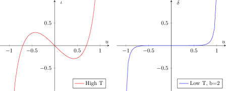
Figure 1: Logarithmic divergence at high and low temperature

(ii) In the low temperature/small box regime $b\gg 1$, it follows from (4.4) that

$$l(\beta,\mu)=\frac{1}{4\pi b^{2}}\sum_{\pm}\Big{[}(4\pi b){\rm Li}_{2}(e^{-(1\mp u)2\pi b})+2{\rm Li}_{3}(e^{-(1\mp u)2\pi b})\Big{]}+\dots,$$ (6.4)

where the dots denote exponentially suppressed contributions. The charge density,

$$\delta(\beta,\mu)=\frac{1}{b}\ln[\frac{1-e^{-(1+u)2\pi b}}{1-e^{-(1-u)2\pi b}}\Big{]}+\mathcal{O}(b^{-2})\dots,$$ (6.5)

again diverges logarithmically at criticality.

Furthermore, this is accompanied by a quantum phase transition. Indeed, $l(\beta,\mu)$ is itself exponentially suppressed when $|u|<1$. At criticality $|u|=1$ however, this exponential suppression turns into a power law. More precisely, the non critical phase with exponential suppression corresponds to $|u|$ sufficiently far from $1$ so that $(1-|u|)2\pi b\gg 1$, while the two critical phases correspond to $|u|$ sufficiently close to $1$ so that $(1-|u|)2\pi b\ll 1$. The cross-over regions are around the lines $(1-|u|)2\pi b=1$. In the critical phases, one may use (4.12) for the expansion of the polylogarithms,

$$l(\beta,\mu)=\frac{1}{b}\Big{[}\zeta(2)|u|+(|u|-1)2\pi b\\ -(|u|-1)2\pi b\ln((1-|u|)2\pi b)+\mathcal{O}((|u|-1)2\pi b)^{2}\Big{]}+\mathcal{O}(b^{-2})+\dots.$$ (6.6)

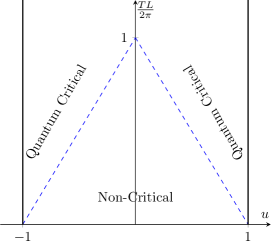
Figure 2: Cross-over regions of the quantum phase transition

The interpretation is as follows. At low temperature/small box, the system is a non-interacting collection in $2$ large spatial dimensions of a massless scalar and complex massive scalars of increasing mass $m_{n}=\frac{2\pi}{L}n$. The singular contribution to the partition function is dominated by the complex scalar with the lowest mass at $n=1$, which determines the critical behavior in this regime.

7 Gravitons

The considerations above generalize directly to the case of gravitons with suitably defined perfectly conducting boundary conditions because the partition function can be shown to be the same as that of photons [22]. In the simple context of free fields, this phase transition for gravitons is a concrete realization of some of the ideas put forward in [24, 25].

8 Discussion

From a theoretical viewpoint, the exact results derived here are closely related to those that appear when generalizing modular invariance from two [26, 27] to higher spacetime dimensions [28, 29, 30, 31], combined with the technique of going back to real rather than purely imaginary chemical potential [32, 33, 34].

The next step consists in studying the effects of adding background curvature and interactions. This should give rise to a more interesting Bose-Einstein condensate and will allow one to study spin effects, that is to say to distinguish between massless scalar fields, photons and gravitons.

References

- [1] H.E. Haber and H.A. Weldon, Thermodynamics of an Ultrarelativistic Bose Gas, Phys. Rev. Lett. 46 (1981) 1497.
- [2] H.E. Haber and H.A. Weldon, Finite Temperature Symmetry Breaking as Bose-Einstein Condensation, Phys.Rev. D25 (1982) 502.
- [3] S. Singh and R.K. Pathria, Bose-Einstein condensation in finite noninteracting systems: A Relativistic gas with pair production, Phys. Rev. A 30 (1984) 442.
- [4] J. Klaers, J. Schmitt, F. Vewinger and M. Weitz, Bose-Einstein condensation of photons in an optical microcavity, Nature 468 (2010) [1007.4088v2].
- [5] R.I. Moodie, P. Kirton and J. Keeling, Polarization dynamics in a photon Bose-Einstein condensate, Phys. Rev. A 96 (2017) 043844.
- [6] H.B. Casimir, On the attraction between two perfectly conducting plates, in Proc. Kon. Ned. Akad. Wet., vol. 51, p. 793, 1948.
- [7] M. Fierz, On the attraction of conducting planes in vacuum, Helv.Phys.Acta 33 (1960) 855.
- [8] J. Mehra, Temperature correction to the Casimir effect, Physica 37 (1967) 145.
- [9] I. Agullo, A. del Rio and J. Navarro-Salas, Electromagnetic duality anomaly in curved spacetimes, Phys. Rev. Lett. 118 (2017) 111301 [1607.08879].
- [10] A. del Rio, N. Sanchis-Gual, V. Mewes, I. Agullo, J.A. Font and J. Navarro-Salas, Spontaneous creation of circularly polarized photons in chiral astrophysical systems, Phys. Rev. Lett. 124 (2020) 211301 [2002.01593].
- [11] M. Fisher and P. De Gennes, Phénomènes aux parois dans un mélange binaire critique, CR Séances Acad. Sci. Paris Ser. B 287 (1978) 207.
- [12] S. Sachdev, Quantum Phase Transitions, Cambridge University Press, 2 ed. (2011), 10.1017/CBO9780511973765.
- [13] A. Gambassi, The Casimir effect: From quantum to critical fluctuations, J. Phys. Conf. Ser. 161 (2009) 012037 [0812.0935].
- [14] D.M. Dantchev and S. Dietrich, Critical Casimir Effect: Exact Results, 2203.15050.
- [15] D.M. Lipkin, Existence of a new conservation law in electromagnetic theory, Journal of Mathematical Physics 5 (1964) 696.
- [16] T.A. Morgan, Two classes of new conservation laws for the electromagnetic field and for other massless fields, Journal of Mathematical Physics 5 (1964) 1659.
- [17] T.W.B. Kibble, Conservation laws for free fields, Journal of Mathematical Physics 6 (1965) 1022.
- [18] M.G. Calkin, An invariance property of the free electromagnetic field, American Journal of Physics 33 (1965) 958 [https://doi.org/10.1119/1.1971089].
- [19] S. Deser and C. Teitelboim, Duality Transformations of Abelian and Nonabelian Gauge Fields, Phys. Rev. D 13 (1976) 1592.
- [20] M.N. Chernodub, A. Cortijo and K. Landsteiner, Zilch vortical effect, Physical Review D 98 (2018) .
- [21] F. Alessio and G. Barnich, Modular invariance in finite temperature Casimir effect, JHEP 10 (2020) 134 [2007.13334].
- [22] F. Alessio, G. Barnich and M. Bonte, Gravitons in a Casimir box, JHEP 02 (2021) 216 [2011.14432].
- [23] H.E. Haber and H.A. Weldon, On the Relativistic Bose-Einstein Integrals, J. Math. Phys. 23 (1982) 1852.
- [24] G. Dvali and C. Gomez, Black Hole’s Quantum N-Portrait, Fortsch. Phys. 61 (2013) 742 [1112.3359].
- [25] G. Dvali and C. Gomez, Black Holes as Critical Point of Quantum Phase Transition, Eur.Phys.J. C74 (2014) 2752 [1207.4059].
- [26] J. Polchinski, Evaluation of the One Loop String Path Integral, Commun. Math. Phys. 104 (1986) 37.
- [27] C. Itzykson and J.B. Zuber, Two-Dimensional Conformal Invariant Theories on a Torus, Nucl. Phys. B 275 (1986) 580.
- [28] A. Cappelli and A. Coste, On the Stress Tensor of Conformal Field Theories in Higher Dimensions, Nucl. Phys. B 314 (1989) 707.
- [29] J.L. Cardy, Operator content and modular properties of higher dimensional conformal field theories, Nucl. Phys. B366 (1991) 403.
- [30] E. Shaghoulian, Modular forms and a generalized Cardy formula in higher dimensions, Phys. Rev. D 93 (2016) 126005 [1508.02728].
- [31] F. Alessio, G. Barnich and M. Bonte, Notes on massless scalar field partition functions, modular invariance and Eisenstein series, JHEP 12 (2021) 211 [2111.03164].
- [32] A. Roberge and N. Weiss, Gauge theories with imaginary chemical potential and the phases of QCD, Nuclear Physics B 275 (1986) 734 .
- [33] M.G. Alford, A. Kapustin and F. Wilczek, Imaginary chemical potential and finite fermion density on the lattice, Phys. Rev. D 59 (1999) 054502 [hep-lat/9807039].
- [34] F. Karbstein and M. Thies, How to get from imaginary to real chemical potential, Phys. Rev. D 75 (2007) 025003.