Estimating Dynamic Games with
Unknown Information Structure

Abstract

This paper studies identification and estimation of dynamic games when the underlying information structure is unknown to the researcher. To tractably characterize the set of model predictions while maintaining weak assumptions on players’ information, we introduce Markov correlated equilibrium, a dynamic analog of Bayes correlated equilibrium. The set of Markov correlated equilibrium predictions coincides with the set of Markov perfect equilibrium predictions that can arise when the players might observe more signals than assumed by the analyst. We characterize the sharp identified sets under varying assumptions on what the players minimally observe. We also propose computational strategies for dealing with the non-convexities that arise in dynamic environments.

Keywords: Dynamic games, Markov correlated equilibrium, informational robustness, partial identification

1 Introduction

This paper develops an empirical framework for estimating a popular class of dynamic games with weak assumptions on players’ information. A series of seminal papers have developed econometric methods for estimating dynamic discrete choice and dynamic games models in a computationally feasible manner (e.g., Rust (1994), Ericson and Pakes (1995), Aguirregabiria and Mira (2007), Bajari, Benkard, and Levin (2007), Pakes, Ostrovsky, and Berry (2007), Pesendorfer and Schmidt-Dengler (2008)), providing toolkits for empirically analyzing strategic interactions in dynamic environments (see Aguirregabiria and Mira (2010) and Aguirregabiria, Collard-Wexler, and Ryan (2021) for recent surveys). However, the empirical models of dynamic games commonly impose a restrictive assumption on players’ information structure, namely that player-specific payoff shocks are private information to each player. While the assumption facilitates computational tractability, it may result in biased estimates due to misspecification. In fact, it is usually difficult for the analyst to know what the players observe or do not observe in a specific empirical context, i.e., the true information structure governing the data generating process remains unknown.

In this paper, we build on a popular class of dynamic games and propose an econometric method for estimating structural parameters while maintaining weak assumption on players’ information. We relax the standard assumption that the analyst knows the exact form of the true information structure. Our approach requires the analyst to only specify the minimal information available to the players. The analyst is open to the possibility that the players might have more information in a form unknown to the analyst. Thus, our framework is “informationally robust” in the sense that it avoids making strong assumptions on players’ information.

The main contributions of this paper are twofold. First, we develop a solution concept dubbed Markov correlated equilibrium as a tool for tractably capturing the set of Markov perfect equilibrium predictions (the joint distribution on actions and states) that can arise when the players might observe more signals than assumed by the analyst. We show that Markov correlated equilibrium is a dynamic Markovian analog of Bayes correlated equilibrium developed by Bergemann and Morris (2013; 2016). Thus, Markov correlated equilibrium inherits the robustness property of Bayes correlated equilibrium.

Second, we propose computationally tractable approaches for estimating the model parameters. We address computational challenges that arise due to the multiplicity of equilibria and dynamic environment. Under our framework, the parameters are usually set identified, which makes standard estimation strategies for dynamic games (e.g., nested fixed-point or CCP-inversion) inapplicable. Furthermore, while computing a Bayes correlated equilibrium is easy as it amounts to solving a linear program, computing a Markov correlated equilibrium is more difficult due to the non-convexities that arise in a dynamic environment. To overcome the computational challenges, we characterize the equilibrium conditions using the one-shot deviation principle and formulate the estimation problem as mathematical programs with equilibrium constraints (Su and Judd (2012) and Egesdal, Lai, and Su (2015a)). We illustrate the performance of our approach via numerical examples.

This paper contributes to the burgeoning literature that develop econometric tools that are robust to misspecification of information structures (Pakes, Porter, Ho, and Ishii (2015), Gualdani and Sinha (2020), Syrgkanis, Tamer, and Ziani (2021), Magnolfi and Roncoroni (2022), Koh (2022)). While Doval and Ely (2020) and Makris and Renou (2021) extend Bayes correlated equilibrium to extensive form games and multi-stage games respectively, this paper limits attention to a class of dynamic games that has served as workhorse models for empirical analysis and exploit the special structure of the model (namely that that the unobserved latent variables are independent over time) to reduce computational burden. To the best of our knowledge, this paper is the first to study informationally robust estimation in a dynamic environment.

The rest of the paper is organized as follows. In Section 2, we establish a connection between Markov correlated equilibria and Markov perfect equilibria in a class of dynamic games and discuss its properties. In Section 3, we introduce an econometric model and discuss informationally robust identification. Section 4 proposes several computational strategies for finding the identified set. Section 5 illustrates the performance of our approach via numerical examples. Section 6 concludes.

Notation.

Throughout the paper, we will use the following notation. If $Y$ is a random variable whose support is a finite set $\mathcal{Y}$, we let $p\left(y\right)\equiv p_{y}\equiv\text{Pr}\left(Y=y\right)$ for $y\in\mathcal{Y}$. Similarly, $p\left(y|x\right)\equiv p_{y|x}\equiv\text{Pr}\left(Y=y|X=x\right)$ denotes the conditional probability of $Y=y$ given $X=x$. We let $\Delta_{y}\equiv\Delta\left(\mathcal{Y}\right)$ denote the probability simplex on $\mathcal{Y}$: $p\in\Delta_{y}$ if and only if $p_{y}\geq 0$ for all $y\in\mathcal{Y}$ and $\sum_{y\in\mathcal{Y}}p_{y}=1$. Similarly, we let $p\in\Delta_{y|x}$ if and only if $p_{y|x}\geq 0$ for each $y\in\mathcal{Y}$ and $\sum_{y\in\mathcal{Y}}p_{y|x}=1$. We also use the convention that writes an action profile as $a=\left(a_{1},...,a_{I}\right)=\left(a_{i},a_{-i}\right)$. For an arbitrary set $S$, $|S|$ represents the cardinality of the set.

2 Model

We consider a class of dynamic Markovian games in infinite-horizon that have been used as a standard framework in the econometrics of dynamic games literature. We first introduce the key concepts in a general environment. Then, we tailor the model when we consider econometric analysis.

2.1 Setup

Let $t=1,2,...,\infty$ denote discrete time. A stationary dynamic Markov game of incomplete information is characterized by a pair of basic game $G$ and information structure $S$. A basic game $G=\langle\mathcal{I},\left(\mathcal{A}_{i},u_{i}\right)_{i\in\mathcal{I}},\mathcal{X},\mathcal{E},\psi,f,\delta\rangle$ specifies payoff-relevant primitives of the model: $i\in\mathcal{I}=\left\{1,2,...,I\right\}$ indexes players; $a_{it}\in\mathcal{A}_{i}$ denotes player $i$’s action at time $t$ where $\mathcal{A}_{i}$ is a finite set of actions available to player $i$; $a_{t}=\left(a_{1t},...,a_{It}\right)\in\mathcal{A}\equiv\times_{i\in\mathcal{I}}\mathcal{A}_{i}$ denotes an action profile; $x_{t}\in\mathcal{X}$ denotes a state variable that is publicly observed by the players, and $\mathcal{X}$ is assumed to be finite; $\varepsilon_{t}\in\mathcal{E}$ denotes a latent state variable that is not directly observed by the players, and $\mathcal{E}$ is assumed to be finite; $\psi\left(\varepsilon_{t}|x_{t}\right)$ represents the players’ prior belief about the probability $\varepsilon_{t}$ conditional on $x_{t}$; $f\left(x_{t+1}|a_{t},x_{t},\varepsilon_{t}\right)$ specifies the probability of transitioning to state $x_{t+1}$ conditional on $\left(a_{t},x_{t},\varepsilon_{t}\right)$; $u_{i}:\mathcal{A}\times\mathcal{X}\times\mathcal{E}\to\mathbb{R}$ is the payoff function of player $i$; $\delta\in[0,1)$ is the common discount factor.

An information structure $S=\langle\left(\mathcal{T}_{i}\right)_{i=1}^{I},\pi\rangle$ specifies information-relevant primitives; $\tau_{it}\in\mathcal{T}_{i}$ denotes player $i$’s private signal at period $t$ where $\mathcal{T}_{i}$ a finite set of private signals; $\tau_{t}=\left(\tau_{1t},...,\tau_{It}\right)\in\mathcal{T}=\times_{i\in\mathcal{I}}\mathcal{T}_{i}$ is a signal profile; $\pi:\mathcal{X}\times\mathcal{E}\to\Delta\left(\mathcal{T}\right)$ is a signal distribution that maps the state of the world to a signal profile, which allows for arbitrary correlation in the private signals. The interpretation is that each player $i$ does not observe the latent state $\varepsilon_{t}$ directly ($x_{t}$ is publicly observed) but each player $i$ receives a private signal $\tau_{it}$ whose informativeness about $\varepsilon_{t}$ depends on $\pi$.

The game $\left(G,S\right)$ is common knowledge to the players. The timing of the model is described as follows. At the beginning of period $t$, the common knowledge state $x_{t}\in\mathcal{X}$ is given and publicly observed. Conditional on $x_{t}$, the latent state $\varepsilon_{t}\in\mathcal{E}$ is drawn from the probability distribution $\psi\left(\cdot|x_{t}\right)$. Next, a profile of private signals $\tau_{t}=\left(\tau_{1t},...,\tau_{It}\right)\in\mathcal{T}$ is drawn from the signal distribution $\pi\left(\cdot|x_{t},\varepsilon_{t}\right)$. At this point, each player $i$ observes $\left(x_{t},\tau_{it}\right)$, which is used to infer the realized latent state $\varepsilon_{t}$ via Bayes’ rule. Then, the players simultaneously determine their actions $a_{it}$, $i=1,...,I$, and each player $i$ receives period $t$ payoff $u_{i}\left(a_{t},x_{t},\varepsilon_{t}\right)$. Finally, the observable state $x_{t}$ transitions to $x_{t+1}$ via the probability kernel $f\left(x_{t+1}|a_{t},x_{t},\varepsilon_{t}\right)$. Given $x_{t+1}$, period $t+1$ begins.

The players are assumed to be rational and forward-looking. In each period $t$, each player $i$ choose action plans to maximize the expected discounted inter-temporal payoffs

$$\mathbb{E}\left\{\sum_{s=t}^{\infty}\delta^{s-t}u_{i}\left(a_{s},x_{s},\varepsilon_{s}\right)|x_{t},\tau_{it}\right\}.$$

The conditioning on $\left(x_{t},\tau_{it}\right)$ reflects the assumption that $i$ observes the public state $x_{t}$ and her signal $\tau_{it}$ before choosing period $t$ action.

Note that the primitives imply that the transition probability of state variables factors as $P_{x_{t+1},\varepsilon_{t+1}|a_{t},x_{t},\varepsilon_{t}}=\psi_{\varepsilon_{t+1}|x_{t+1}}f_{x_{t+1}|a_{t},x_{t},\varepsilon_{t}}$. The assumption that the latent variables are generated independently of the states in the previous period is standard in the empirical literature and is crucial for simplifying the computation of equilibria. This assumption will also play a vital role in this paper by allowing us to directly leverage Theorem 1 of Bergemann and Morris (2016) in characterizing the set of robust predictions in a dynamic environment.

Example 1 (Two-player dynamic entry game).

Let us consider a two-player entry game example. Players’ decisions are binary with $a_{it}=0$ if firm $i$ is not active in the market and $a_{it}=1$ if active. The endogenous state variable is the lagged decision $z_{it}=a_{it-1}$, which determines the firm’s incumbency status. A potential entrant pays an entry cost if it enters the market. An incumbent does not pay an entry cost to stay active, but receives a scrap value (or pays an exit cost) upon exiting. An active firm receives an operating profit that may be affected by the opponents’ presence in the market. The per-period payoff can be summarized as

$$u_{i}\left(a_{it},a_{jt},z_{it},\varepsilon_{it}\right)=\begin{cases}MP\times\mathbb{I}\left\{a_{jt}=0\right\}+DP\times\mathbb{I}\left\{a_{jt}=1\right\}+EC\times\mathbb{I}\left\{z_{it}=0\right\}+\varepsilon_{it}&\text{if }a_{it}=1\\ SV\times\mathbb{I}\left\{z_{it}=1\right\}&\text{if }a_{it}=0\end{cases}$$

where $MP$ denotes monopoly profit, $DP$ duopoly profit, $EC$ entry cost, and $SV$ scrap value. $\varepsilon_{it}\in\mathbb{R}$ represents an idiosyncratic shock to the operating profit. In this example, the observable state is $x_{t}=\left(z_{1t},z_{2t}\right)\in\mathbb{R}^{2}$ and the latent state is $\varepsilon_{t}=\left(\varepsilon_{1t},\varepsilon_{2t}\right)\in\mathbb{R}^{2}$.

A common assumption used in the empirical literature is that $\varepsilon_{it}$ is privately observed by $i$. We denote such information structure by $S^{\varepsilon_{i}}$. Formally, $S^{\varepsilon_{i}}$ is described by a signal space $\mathcal{T}_{i}=\mathcal{E}_{i}$ and a signal distribution that places unit mass on the event that $\tau_{i}=\varepsilon_{i}$ for each player $i$. Other information structures can be considered. For example, $S^{null}$ represents an information structure in which each player receives no (null) signal about the realization of $\varepsilon_{t}$. Under $S^{null}$, each player only relies on its observation of $x_{t}$ and its knowledge about the prior distribution of $\varepsilon_{t}$ to make decisions. $\blacksquare$

2.2 Markov Perfect Equilibrium

From now on, we suppress time subscripts unless necessary since the environment is stationary. A Markov strategy of player $i$ is a mapping $\beta_{i}:\mathcal{X}\times\mathcal{T}_{i}\to\Delta\left(\mathcal{A}_{i}\right)$ that specifies a probability distribution over actions at each realization of observable state and private signal. A strategy profile $\beta=\left(\beta_{1},...,\beta_{I}\right)$ is a Markov perfect equilibrium if for each player $i$, any action on the support of $\beta_{i}$ maximizes $i$’s expected discounted sum of payoffs given that all players behave optimally now and in the future.

Definition 1 (Markov Perfect Equilibrium).

A strategy profile $\beta$ is a Markov perfect equilibrium of $\left(G,S\right)$ if there exists $\left\{\tilde{V}_{i}\left(x,\tau_{i}\right)\right\}_{\left(i,x,\tau_{i}\right)\in\mathcal{I}\times\mathcal{X}\times\mathcal{T}_{i}}$ such that

1. (Bellman) For all $i\in\mathcal{I}$, $x\in\mathcal{X}$, $\tau_{i}\in\mathcal{T}_{i}$,

   $$\tilde{V}_{i}\left(x,\tau_{i}\right)=\max_{\tilde{a}_{i}\in\mathcal{A}_{i}}\mathbb{E}_{\left(a_{-i},\varepsilon\right)}^{\beta}\left\{u_{i}\left(\tilde{a}_{i},a_{-i},x,\varepsilon\right)+\delta\sum_{x^{\prime},\tau_{i}^{\prime}}P_{x^{\prime},\tau_{i}^{\prime}|\tilde{a}_{i},a_{-i},x,\varepsilon}\tilde{V}_{i}\left(x^{\prime},\tau_{i}^{\prime}\right)\bigg{|}x,\tau_{i}\right\}$$ (1)

   where the expectation is taken over $a_{-i}$ and $\varepsilon$.

2. (Optimality) For all $i\in\mathcal{I}$, $x\in\mathcal{X}$, $\tau_{i}\in\mathcal{T}_{i}$, $\beta_{i}\left(a_{i}|x,\tau_{i}\right)>0$ implies

   $$a_{i}=\arg\max_{\tilde{a}_{i}\in\mathcal{A}_{i}}\mathbb{E}_{\left(a_{-i},\varepsilon\right)}^{\beta}\left\{u_{i}\left(\tilde{a}_{i},a_{-i},x,\varepsilon\right)+\delta\sum_{x^{\prime},\tau_{i}^{\prime}}P_{x^{\prime},\tau_{i}^{\prime}|\tilde{a}_{i},a_{-i},x,\varepsilon}\tilde{V}_{i}\left(x^{\prime},\tau_{i}^{\prime}\right)\bigg{|}x,\tau_{i}\right\}.$$ (2)

Equation (1) says that each $\tilde{V}_{i}\left(x,\tau_{i}\right)\in\mathbb{R}$ represents $i$’s value function at information set $\left(x,\tau_{i}\right)$ when the players are following $\beta$. Equation (2) says that each action on the support of $\beta_{i}$ maximizes $i$’s discounted sum of payoffs computed using the value functions.

One-shot Deviation Principle

We restate Definition 1 using the one-shot deviation principle, which states that $\beta$ is an equilibrium strategy profile if and only if there exists no player and an information set at which a one-shot deviation can be profitable. There are two advantages associated with the reformulation. First, by formulating Markov perfect equilibrium as a Bayes Nash equilibrium of a reduced normal form game induced by a strategy profile, we can leverage results from the static environment. Second, the formulation facilitates computation.

Any strategy profile $\beta=\left(\beta_{1},...,\beta_{I}\right)$ induces an ex-ante value function $V_{i}^{\beta}\in\mathbb{R}^{|\mathcal{X}|}$. Each $V_{i}^{\beta}\left(x\right)$ captures $i$’s expected payoff at state $x$ before the realization of $\varepsilon$ given that all players follow the prescriptions in $\beta$. For each $i$, $V_{i}^{\beta}$ is the unique solution to

$$V_{i}^{\beta}\left(x\right)=\sum_{\varepsilon\in\mathcal{E},\tau\in\mathcal{T},a\in\mathcal{A}}\psi_{\varepsilon|x}\pi_{\tau|x,\varepsilon}\beta_{a|x,\tau}\left\{u_{i}\left(a,x,\varepsilon\right)+\delta\sum_{x^{\prime}\in\mathcal{X}}V_{i}^{\beta}\left(x^{\prime}\right)f_{x^{\prime}|a,x,\varepsilon}\right\},\quad\forall i\in\mathcal{I},x\in\mathcal{X}.$$ (3)

where $\beta_{a|x,\tau}\equiv\prod_{j=1}^{I}\beta_{j}\left(a_{j}|x,\tau_{j}\right)$ denotes the conditional distribution over action profiles induced by the strategy profile $\beta$.

Define the outcome-specific function given $\beta$ as

$$v_{i}^{\beta}\left(a,x,\varepsilon\right)\equiv u_{i}\left(a,x,\varepsilon\right)+\delta\sum_{x^{\prime}\in\mathcal{X}}V_{i}^{\beta}\left(x^{\prime}\right)f_{x^{\prime}|a,x,\varepsilon}.$$

The outcome-specific function represents the continuation payoff to player $i$ is $\left(a,x,\varepsilon\right)$ is realized today and all players follow the prescriptions in $\beta$ from tomorrow and onward.

A strategy profile $\beta$ induces a reduced normal form (basic) game $G^{\beta}=\langle\mathcal{I},\left(\mathcal{A}_{i},v_{i}^{\beta}\right)_{i\in\mathcal{I}},\mathcal{X},\mathcal{E},\psi\rangle$. Then $\left(G^{\beta},S\right)$ describes a “static” game in which player $i$’s payoff function is given by $v_{i}^{\beta}\left(a,x,\varepsilon\right)$. The following lemma, which is based on the one-shot deviation principle, allows us to bring the results in static environments to dynamic environments.

Lemma 1.

A strategy profile $\beta$ is a Markov perfect equilibrium of $\left(G,S\right)$ if and only if $\beta$ is a Bayes Nash equilibrium of $\left(G^{\beta},S\right)$.

2.3 Markov Correlated Equilibrium

Decision Rule

A stationary Markov decision rule in $\left(G,S\right)$ is a mapping

$$\sigma:\mathcal{X}\times\mathcal{E}\times\mathcal{T}\to\Delta\left(\mathcal{A}\right),$$

which specifies a probability distribution over action profiles at each realization of state of the world and players’ signals.

It is instructive to think of $\sigma$ as a recommendation strategy of an omniscient mediator who observes $\left(x,\varepsilon,\tau\right)$ and privately recommends actions to each player. Suppose that the mediator commits to a stationary recommendation strategy $\sigma$ and announces it to the players. After the state and players’ signals $\left(x,\varepsilon,\tau\right)$ are realized, an action profile $a=\left(a_{1},...,a_{I}\right)$ is drawn from the probability distribution $\sigma\left(\cdot|x,\varepsilon,\tau\right)$, and each $a_{i}$ is privately recommended to each player $i$. Each player $i$, having observed $\left(x,\tau_{i},a_{i}\right)$, decides whether to obey (play $a_{i}$) or not (deviate to $a_{i}^{\prime}\neq a_{i}$). If $\sigma$ is such that the players are always obedient, we call $\sigma$ a Markov correlated equilibrium of $\left(G,S\right)$.

Definition

To formalize the equilibrium condition, let us introduce some notation. Let $V_{i}^{\sigma}\in\mathbb{R}^{|\mathcal{X}|}$ denote the ex-ante value function induced by $\sigma$. $V_{i}^{\sigma}$ is obtained as the unique solution to

$$V_{i}^{\sigma}\left(x\right)=\sum_{\varepsilon\in\mathcal{E},\tau\in\mathcal{T},a\in\mathcal{A}}\psi_{\varepsilon|x}\pi_{\tau|x,\varepsilon}\sigma_{a|x,\varepsilon,\tau}\left\{u_{i}\left(a,x,\varepsilon\right)+\delta\sum_{x^{\prime}\in\mathcal{X}}V_{i}^{\sigma}\left(x^{\prime}\right)f_{x^{\prime}|a,x,\varepsilon}\right\},\quad\forall x\in\mathcal{X}.$$

Also define the outcome-specific function associated with $\sigma$ as

$$v_{i}^{\sigma}\left(a,x,\varepsilon\right):=u_{i}\left(a,x,\varepsilon\right)+\delta\sum_{x^{\prime}\in\mathcal{X}}V_{i}^{\sigma}\left(x^{\prime}\right)f_{x^{\prime}|a,x,\varepsilon},$$

which represents the payoff to player $i$ if $\left(a,x,\varepsilon\right)$ is realized today and the players’ actions are determined by $\sigma$ in the future.

Let $\mathbb{E}^{\sigma}\left[v_{i}^{\sigma}\left(\tilde{a}_{i},a_{-i},x,\varepsilon\right)|x,\tau_{i},a_{i}\right]$ be the expected payoff to player $i$ from choosing $\tilde{a}_{i}$ when $i$ observes $\left(x,\tau_{i}\right)$ and receives a recommendation $a_{i}$. The following definition states that $\sigma$ is a Markov correlated equilibrium of $\left(G,S\right)$ if the players do not have incentives to deviate from the mediator’s recommendations.

Definition 2.

A decision rule $\sigma$ is a Markov correlated equilibrium of $\left(G,S\right)$ if for each $i\in\mathcal{I},x\in\mathcal{X},\tau_{i}\in\mathcal{T}_{i}$, and $a_{i}\in\mathcal{A}_{i}$, we have

$$\mathbb{E}^{\sigma}\left[v_{i}^{\sigma}\left(a_{i},a_{-i},x,\varepsilon\right)|x,\tau_{i},a_{i}\right]\geq\mathbb{E}^{\sigma}\left[v_{i}^{\sigma}\left(\tilde{a}_{i},a_{-i},x,\varepsilon\right)|x,\tau_{i},a_{i}\right]$$ (4)

for each $\tilde{a}_{i}\neq a_{i}$ whenever $\text{Pr}^{\sigma}\left(x,t_{i},a_{i}\right)>0$.

Since

$$\mathbb{E}^{\sigma}\left[v_{i}\left(\tilde{a}_{i},a_{-i},x,\varepsilon\right)|x,\tau_{i},a_{i}\right] =\sum_{\varepsilon,a_{-i}}v_{i}^{\sigma}\left(\tilde{a}_{i},a_{-i},x,\varepsilon\right)\text{Pr}^{\sigma}\left(\varepsilon,a_{-i}|x,\tau_{i},a_{i}\right)$$

$$=\sum_{\varepsilon,a_{-i}}v_{i}^{\sigma}\left(\tilde{a}_{i},a_{-i},x,\varepsilon\right)\left(\frac{\sum_{\tau_{-i}}\psi_{\varepsilon|x}\pi_{\tau|x,\varepsilon}\sigma_{a|x,\varepsilon,\tau}}{\sum_{\varepsilon,\tau_{-i},a_{-i}}\psi_{\varepsilon|x}\pi_{\tau|x,\varepsilon}\sigma_{a|x,\varepsilon,\tau}}\right),$$

after cancelling out the denominator, which is constant across all possible realizations of $\left(\varepsilon,\tau_{-i},a_{-i}\right)$, (4) can be rewritten as:

$$\sum_{\varepsilon,\tau_{-i},a_{-i}}\psi_{\varepsilon|x}\pi_{\tau|x,\varepsilon}\sigma_{a|x,\varepsilon,\tau}v_{i}^{\sigma}\left(a,x,\varepsilon\right)\geq\sum_{\varepsilon,\tau_{-i},a_{-i}}\psi_{\varepsilon|x}\pi_{\tau|x,\varepsilon}\sigma_{a|x,\varepsilon,\tau}v_{i}^{\sigma}\left(\tilde{a}_{i},a_{-i},x,\varepsilon\right),\quad\forall i,\tau_{i},a_{i},\tilde{a}_{i}.$$ (5)

As before, an arbitrary $\sigma$ in $\left(G,S\right)$ induces a reduced normal form game $\left(G^{\sigma},S\right)$ where $G^{\sigma}=\langle\mathcal{I},\left(\mathcal{A}_{i},v_{i}^{\sigma}\right),\mathcal{X},\mathcal{E},\psi\rangle$. Then (5) shows that if $\sigma$ is a Markov correlated equilibrium of $\left(G,S\right)$, it is a Bayes correlated equilibrium of the reduced-form game $\left(G^{\sigma},S\right)$ induced by $\sigma$.

Lemma 2.

A decision rule $\sigma$ is a Markov correlated equilibrium of $\left(G,S\right)$ if and only if $\sigma$ is a Bayes correlated equilibrium of $\left(G^{\sigma},S\right)$.

Comparison to Bayes correlated equilibrium

When $\delta=0$, Markov correlated equilibrium collapses to Bayes correlated equilibrium:

$$\sum_{\varepsilon,\tau_{-i},a_{-i}}\psi_{\varepsilon|x}\pi_{\tau|x,\varepsilon}\sigma_{a|x,\varepsilon,\tau}u_{i}\left(a,x,\varepsilon\right)\geq\sum_{\varepsilon,\tau_{-i},a_{-i}}\psi_{\varepsilon|x}\pi_{\tau|x,\varepsilon}\sigma_{a|x,\varepsilon,\tau}u_{i}\left(\tilde{a}_{i},a_{-i},x,\varepsilon\right),\quad\forall i,\tau_{i},a_{i},\tilde{a}_{i}.$$ (6)

Thus, the former is a proper dynamic analog of the latter.

Unfortunately, however, contrary its static analog (6), the Markov correlated equilibrium conditions (5) are not linear with respect to the decision rule $\sigma$. The non-linearity introduces challenges that are absent in the static case. First, whereas computing a Bayes correlated equilibrium amounts to solving a linear program, computing a Markov correlated equilibrium generally requires solving a non-convex program. Second, the set of Bayes correlated equilibria is convex, but the set of Markov correlated equilibria is generally non-convex. The convexity of the set of Bayes correlated equilibria implies that it is without loss to assume that the data are generated by a mixture of multiple equilibria in the static case when conducting econometric analysis. In contrast, in the dynamic case, the econometrician needs to impose a single equilibrium assumption (which is still a standard assumption in the econometrics of dynamic games literature) in order to keep computation tractable.

2.4 Informational Robustness of Markov Correlated Equilibrium

Partial Ordering of Information Structures

To discuss the informational robustness property of Markov correlated equilibrium, we use a partial order on the set of information structures. Specifically, we use the notion of expansion, defined in BM, which orders information structures based on the level of informativeness of the signals. Let $\omega\in\Omega\equiv\mathcal{X}\times\mathcal{E}$ denote the state of the world.

Definition 3 (Expansion).

Let $S=\left(\mathcal{T},\pi\right)$ be an information structure. $S^{*}=\left(\mathcal{T}^{*},\pi^{*}\right)$ is an expansion of $S$, or $S^{*}\succsim_{E}S$, if there exists $\left(\tilde{\mathcal{T}}_{i}\right)_{i=1}^{I}$ and $\lambda:\Omega\times\mathcal{T}\to\Delta\left(\tilde{\mathcal{T}}\right)$ such that $\mathcal{T}_{i}^{*}=\mathcal{T}_{i}\times\tilde{\mathcal{T}}_{i}$ for all $i=1,...,I$ and $\pi^{*}\left(\tau,\tilde{\tau}|\omega\right)=\pi\left(\tau|\omega\right)\lambda\left(\tilde{\tau}|\omega,\tau\right)$.

Intuitively, if $S^{*}\succsim_{E}S$, then the players, under $S^{*}$, get to observe extra signals generated by $\lambda$ in addition to the signals in $S$.

Reduced Normal Form Games

Let $\beta=\left(\beta_{i}\right)_{i\in\mathcal{I}}$ be a strategy profile in $\left(G,S^{*}\right)$ where $\beta_{i}:\mathcal{X}\times\mathcal{T}_{i}\times\tilde{\mathcal{T}}_{i}\to\Delta\left(\mathcal{A}_{i}\right)$. We say $\beta$ induces a decision rule $\sigma$ for $\left(G,S\right)$ if

$$\sigma\left(a|x,\varepsilon,\tau\right)=\sum_{\tilde{\tau}\in\tilde{\mathcal{T}}}\lambda\left(\tilde{\tau}|x,\varepsilon,\tau\right)\prod_{j=1}^{I}\beta_{j}\left(a_{j}|x,\tau_{j},\tilde{\tau}_{j}\right),\quad\forall a,x,\varepsilon,\tau.$$

The following lemma states that if $\beta$ induces $\sigma$, then the associated reduced-form games, $G^{\beta}$ and $G^{\sigma}$, are identical.

Lemma 3.

If $\beta$ induces $\sigma$, then the associated reduced normal form games, $G^{\beta}$ and $G^{\sigma}$, are identical.

Lemma 3 is intuitive: if $\beta$ induces $\sigma$, then $\beta$ and $\sigma$ induce identical distributions over action profiles at each state of the world, so the associated ex-ante value functions must be identical to each other, i.e., $V_{i}^{\beta}=V_{i}^{\sigma}$. Then, the outcome-specific payoff functions are also identical to each other, i.e., $v_{i}^{\beta}=v_{i}^{\sigma}$, making all primitives of the basic game identical to each other.

Informational Robustness of Markov Correlated Equilibrium

Our main theorem states that the set of Markov correlated equilibrium of a game $\left(G,S\right)$ captures the implications of Markov perfect equilibrium when the players might observe more signals. Our result is a dynamic Markovian analog of Theorem 1 of BM.

A solution concept generates a prediction defined as a probability distribution over actions at each realized state and signal. Let $\mathcal{P}_{a|x,\varepsilon,\tau}^{MPE}\left(G,S\right)$ denote the set of predictions that can be induced by a Markov perfect equilibrium in $\left(G,S\right)$. Let $\mathcal{P}_{a|x,\varepsilon,\tau}^{MCE}\left(G,S\right)$ be defined similarly.

Theorem 1 (Informational Robustness).

For any basic game $G$ and information structure $S$,

$$\mathcal{P}_{a|x,\varepsilon,\tau}^{MCE}\left(G,S\right)=\bigcup_{S^{*}\succsim_{E}S}\mathcal{P}_{a|x,\varepsilon,\tau}^{MPE}\left(G,S^{*}\right).$$

Theorem 1 is useful because $\mathcal{P}_{a|x,\varepsilon,\tau}^{MCE}\left(G,S\right)$ is far easier to characterize than $\bigcup_{S^{*}\succsim_{E}S}\mathcal{P}_{a|x,\varepsilon,\tau}^{MPE}$ as the former does not require searching over the set of information structures.

In the econometric analysis, it is common to assume that the analyst observes the conditional choice probabilities that represent the probability of each action profile at each state that is observable to the analyst. Thus, it is useful to characterize the implications of Theorem 1 in terms of conditional choice probabilities. Let $\mathcal{P}_{a|x}^{MPE}\left(G,S\right)$ denote the set of feasible conditional choice probabilities that can arise under a Markov perfect equilibrium of $\left(G,S\right)$. Let $\mathcal{P}_{a|x}^{MCE}\left(G,S\right)$ be defined similarly.

Corollary 1.

For any basic game $G$ and information structure $S$,

$$\mathcal{P}_{a|x}^{MCE}\left(G,S\right)=\bigcup_{S^{*}\succsim S}\mathcal{P}_{a|x}^{MPE}\left(G,S^{*}\right).$$

3 Econometric Model and Identification

Let us specialize the model by imposing assumptions that facilitate econometric analysis. We study the identification problem while being agnostic about the underlying information structure of the game.

3.1 Setup

Let the latent state be a vector of player-specific shocks, i.e., $\varepsilon\equiv\left(\varepsilon_{1},\varepsilon_{2},...,\varepsilon_{I}\right)$ and $\varepsilon_{i}\in\mathcal{E}_{i}$ only enters player $i$’s payoff. Assume that the payoff functions and the prior distribution are parameterized by a finite-dimensional vector $\theta$ so that $u_{i}=u_{i}^{\theta}$ and $\psi=\psi^{\theta}$. We also assume $f_{x^{\prime}|a,x,\varepsilon}=f_{x^{\prime}|a,x}$, i.e., the transition probabilities of observable states are independent of the latent variable $\varepsilon$.

The econometrician observes data

$$\left\{a_{m,t},x_{m,t}:\ m=1,2,...,M,\ t=1,2,...,T\right\},$$

which have players’ actions $a_{m,t}$ and common knowledge state variables $x_{m,t}$ across $M$ independent markets over $T$ periods. We assume that $M$ is large and that the conditional choice probabilities $\phi:\mathcal{X}\to\Delta\left(\mathcal{A}\right)$ and the transitional probability function $f:\mathcal{A}\times\mathcal{X}\to\Delta\left(\mathcal{X}\right)$ can be non-parametrically identified from the data. Finally we assume that the common discount factor $\delta\in[0,1)$ is known to the researcher.

We summarize the baseline assumptions for econometric analysis as follows.

Assumption 1 (Baseline assumptions for identification).

1. The set of covariates $\mathcal{X}$ and the set of latent states $\mathcal{E}$ are finite.

2. The prior distribution $\psi^{\theta}$ and the payoff functions $u_{i}^{\theta}$ are known up to a finite-dimensional parameter $\theta$.

3. The state of the world is a vector of player-specific payoff shocks, i.e., $\varepsilon=\left(\varepsilon_{1},...,\varepsilon_{I}\right)$ and $u_{i}^{\theta}\left(a,x,\varepsilon\right)=u_{i}^{\theta}\left(a,x,\varepsilon_{i}\right)$. The transition probability of observable states is independent of the latent state, i.e., $f_{x^{\prime}|a,x,\varepsilon}=f_{x^{\prime}|a,x}$.

4. The conditional choice probabilities $\phi:\mathcal{X}\to\Delta\left(\mathcal{A}\right)$ and the transition probability function $f:\mathcal{A}\times\mathcal{X}\to\Delta\left(\mathcal{A}\right)$ are identified from the data.

The only “unconventional” assumption is that $\mathcal{E}$ is finite. One may understand this assumption as discretizing the space of latent variables for estimation to be feasible. The discretization of state space for feasible estimation is also used in Gualdani and Sinha (2020), Magnolfi and Roncoroni (2022), and Syrgkanis, Tamer, and Ziani (2021).

Identified Set

Let $\left(G^{\theta},S\right)$ be a dynamic game of incomplete information. Given a solution concept $SC$, which restricts the set of model predictions, the identified set of parameters is defined as follows.

Definition 4 (Identified set).

Given Assumption 1, a solution concept $SC$, and information structure $\tilde{S}$, the identified set of parameters is defined as:

$$\Theta_{I}^{SC}\left(\tilde{S}\right)\equiv\left\{\theta\in\Theta:\ \phi\in\mathcal{P}_{a|x}^{SC}\left(G^{\theta},\tilde{S}\right)\right\}.$$

In words, a candidate parameter $\theta$ enters the identified set $\Theta_{I}^{SC}\left(\tilde{S}\right)$ if the observed CCPs $\phi$ can be rationalized by some equilibrium (defined via a solution concept) of the model.

3.2 Informationally Robust Identified Set

Consider the following assumption which states that the data are generated by a Markov perfect equilibrium under some information structure that is an expansion of a baseline information structure denoted $S$.

Assumption 2 (Identification under Markov perfect equilibrium).

The data are generated by a Markov perfect equilibrium of $\left(G^{\theta_{0}},\tilde{S}^{0}\right)$ for some information structure $\tilde{S}^{0}$ that is an expansion of $S$.

We will consider a scenario where the true information structure that generates the data is $\tilde{S}^{0}$, but the researcher only knows some $S$ for which $\tilde{S}^{0}\succsim_{E}S$. That is, the researcher knows some minimal information available to the players. For instance, the analyst might know that each player $i$ observes at least $\varepsilon_{i}$, although she does not know whether the players have access to more information (Magnolfi and Roncoroni (2022) uses this assumption for econometric analysis in static environment). Then, in principle, the analyst should check whether there exists some Markov perfect equilibrium under some information structure $\tilde{S}\succsim_{E}S^{\varepsilon_{i}}$ that can rationalize the data. Clearly, such task is computationally infeasible because the set of information structures is too large.

Fortunately, it turns out that we can replace Assumption 2 with the following assumption to make the task computationally feasible.

Assumption 3 (Identification under Markov correlated equilibrium).

The data are generated by a Markov correlated equilibrium of $\left(G^{\theta_{0}},S\right)$.

Theorem 2 (Equivalence of identified sets).

The identified set under Assumptions 1 and 2 is equal to the identified set under Assumptions 1 and 3.

Theorem 2 says that, if the researcher knows that the data are generated by a Markov perfect equilibrium but does not know the underlying information structure, the researcher can proceed by treating the data as if they were generated from a Markov correlated equilibrium. Similar results have been obtained by Gualdani and Sinha (2020), Magnolfi and Roncoroni (2022), and Syrgkanis, Tamer, and Ziani (2021) in static environments to leverage the informational robustness and computational tractability of Bayes correlated equilibrium. Theorem 2 extends the result to a popular class of dynamic Markov games.

Equilibrium Selection

In the static case, the assumption that the data are generated by a single equilibrium is without loss since a mixture of Bayes correlated equilibria is also a Bayes correlated equilibrium (see Magnolfi and Roncoroni (2022) and Syrgkanis, Tamer, and Ziani (2021)). However, this property does not carry over to the dynamic case because a mixture of Markov correlated equilibria is not necessarily a Markov correlated equilibrium. Although we do not assume a particular equilibrium selection rule, we assume that the data are generated by a single Markov perfect equilibrium. Identification under arbitrary equilibrium selection rule is possible (e.g., Beresteanu, Molchanov, and Molinari (2011)), but more complicated.

4 Computational Strategies

Computing the sharp identified set can be computationally challenging. We propose multiple computational strategies for feasible estimation.

4.1 Sharp Identified Set

Fix an information structure $S$, and let $\Theta_{I}\equiv\Theta_{I}^{MCE}\left(S\right)$. Suppose, for a given candidate parameter $\theta$, we want to test whether $\theta$ enters $\Theta_{I}$. Let $\partial v_{i}^{\theta}\left(\tilde{a}_{i},a,x,\varepsilon_{i}\right)\equiv v_{i}^{\theta}\left(\tilde{a}_{i},a_{-i},x,\varepsilon_{i}\right)-v_{i}^{\theta}\left(a,x,\varepsilon_{i}\right)$ denote the profit from deviating to $\tilde{a}_{i}$ when the original action is $a_{i}$. The following theorem provides an operational characterization of the identified set by formulating the identification problem as a mathematical program with equilibrium constraints (Su and Judd, 2012).

Theorem 3 (Sharp identified set).

$\theta\in\Theta_{I}$ if and only if there exists $\sigma:\mathcal{X}\times\mathcal{E}\times\mathcal{T}\to\Delta\left(\mathcal{A}\right)$ and $V=\left(V_{i,x}\right)_{i\in\mathcal{I},x\in\mathcal{X}}\in\mathbb{R}^{|\mathcal{I}|\times|\mathcal{X}|}$ such that

$$\sum_{\varepsilon,\tau_{-i},a_{-i}}\psi_{\varepsilon|x}\pi_{\tau|x,\varepsilon}\sigma_{a|x,\varepsilon,\tau}\partial v_{i}^{\theta}\left(\tilde{a}_{i},a,x,\varepsilon_{i}\right)\leq 0,\quad\forall x,\tau_{i},a_{i},\tilde{a}_{i}$$ (7)

$$v_{i}^{\theta}\left(a,x,\varepsilon_{i}\right)=u_{i}^{\theta}\left(a,x,\varepsilon_{i}\right)+\delta\sum_{x^{\prime}}V_{i,x^{\prime}}f_{x^{\prime}|a,x},\quad\forall i,a,x,\varepsilon_{i}$$ (8)

$$V_{i,x}=\sum_{\varepsilon,\tau,a}\psi_{\varepsilon|x}\pi_{\tau|a,x}\sigma_{a|x,\varepsilon,\tau}u_{i}^{\theta}\left(a,x,\varepsilon_{i}\right)+\delta\sum_{a,x^{\prime}}\phi_{a|x}f_{x^{\prime}|a,x}V_{i,x^{\prime}},\quad\forall i,x$$ (9)

$$\phi_{a|x}=\sum_{\varepsilon,\tau}\psi_{\varepsilon|x}\pi_{\tau|a,x}\sigma_{a|x,\varepsilon,\tau},\quad\forall a,x$$ (10)

In the above, (7)–(9) represent the Markov correlated equilibrium conditions, and (10) represents the consistency requirement that $\sigma$ induces the CCPs observed in the data. Note that (i) $\sigma:\mathcal{X}\times\mathcal{E}\times\mathcal{T}\to\Delta\left(\mathcal{A}\right)$ translates to the requirement that $\sigma_{a|x,\varepsilon,\tau}\geq 0$ for all $a,x,\varepsilon,\tau$ and $\sum_{a}\sigma_{a|x,\varepsilon,\tau}=1$ for all $x,\varepsilon,\tau$ which are linear constraints; (ii) $v_{i}^{\theta}\left(a,x,\varepsilon_{i}\right)$ is an auxiliary expression, and (iii) (9) is obtained by imposing (10) in the equations for ex ante value functions. Thus, to test where $\theta\in\Theta_{I}$, the analyst solves a non-convex program whose variables of optimization are $\sigma$ and $V$, and the non-convexity arises from the bilinearity of (7) with respect to $\sigma$ and $V$.

Theorem 3 also shows that we can find the projection intervals of $\Theta_{I}$ by solving nonlinear programs. Specifically, to find the projections of $\Theta_{I}$ in direction $p\in\mathbb{R}^{\dim\left(\theta\right)}$, one can solve

$$\min_{\theta,\sigma,V}p^{T}\theta$$

subject to the constraints in Theorem 3.

Example 2.

When the baseline information structure is set to $S=S^{\varepsilon_{i}}$, the program in Theorem 3 reduces to: find $\sigma:\mathcal{X}\times\mathcal{E}\to\Delta\left(\mathcal{A}\right)$ and $V_{i}\in\mathbb{R}^{|\mathcal{X}|}$ for $i=1,...,I$ such that

$$\sum_{\varepsilon_{-i},a_{-i}}\psi_{\varepsilon|x}\sigma_{a|x,\varepsilon}\partial v_{i}^{\theta}\left(\tilde{a}_{i},a,x,\varepsilon_{i}\right)\leq 0,\quad\forall i,x,\varepsilon_{i},a_{i},\tilde{a}_{i}$$

$$v_{i}^{\theta}\left(a,x,\varepsilon_{i}\right)=u_{i}^{\theta}\left(a,x,\varepsilon_{i}\right)+\delta\sum_{x^{\prime}}f_{x^{\prime}|a,x}V_{i,x^{\prime}},\quad\forall i,a,x,\varepsilon_{i}$$

$$V_{i,x}=\sum_{\varepsilon,a}\psi_{\varepsilon|x}\sigma_{a|x,\varepsilon}u_{i}^{\theta}\left(a,x,\varepsilon_{i}\right)+\delta\sum_{a,x^{\prime}}\phi_{a|x}f_{x^{\prime}|a,x}V_{i,x^{\prime}},\quad\forall i,x$$

$$\phi_{a|x}=\sum_{\varepsilon}\psi_{\varepsilon|x}\sigma_{a|x,\varepsilon},\quad\forall a,x.$$

$\blacksquare$

A Criterion Function Approach

It is useful to take the following approach which computes a criterion function $Q:\Theta\mapsto\mathbb{R}_{+}$ such that $\theta\in\Theta_{I}$ if and only if $Q\left(\theta\right)=0$.

$$Q\left(\theta\right):\quad\min_{t,V,\sigma}t\quad\text{subject to}$$ (11)

$$\sum_{\varepsilon,\tau_{-i},a_{-i}}\psi_{\varepsilon|x}\pi_{\tau|x,\varepsilon}\sigma_{a|x,\varepsilon,\tau}\left(\partial u_{i}^{\theta}\left(\tilde{a}_{i},a,x,\varepsilon_{i}\right)+\delta\sum_{x^{\prime}}V_{i,x^{\prime}}\partial f_{x^{\prime}|\tilde{a}_{i},a,x}\right)\leq t,\quad\forall i,x,\tau_{i},a_{i},\tilde{a}_{i}$$

$$V_{i,x}=\sum_{\varepsilon,\tau,a}\psi_{\varepsilon|x}\pi_{\tau|a,x}\sigma_{a|x,\varepsilon,\tau}u_{i}^{\theta}\left(a,x,\varepsilon_{i}\right)+\delta\sum_{a,x^{\prime}}\phi_{a|x}f_{x^{\prime}|a,x}V_{i,x^{\prime}},\quad\forall i,x$$

$$t\geq 0,\quad\phi=\phi\left(\sigma\right),\quad\sigma\in\Delta_{a|x,\varepsilon,\tau}$$

where $\phi=\phi\left(\sigma\right)$ is a shorthand for the consistency condition and $\sigma\in\Delta_{a|x,\varepsilon,\tau}$ is a shorthand for the condition that requires $\sigma$ be proper conditional probability distributions.

Theorem 4 (Criterion function approach).

For any $\theta\in\Theta$, (11) is feasible. Furthermore, $Q\left(\theta\right)=0$ if and only if $\theta\in\Theta_{I}$.

4.2 Fully Robust Set

In the special case where $S$ is set to $S^{null}$ (i.e., the analyst assumes no minimal information), determining whether $\theta$ enters the identified set is more tractable since it amounts to solving a linear program.

When $S=S^{null}$, the identification conditions collapse to

$$\sum_{\varepsilon,a_{-i}}\psi_{\varepsilon|x}\sigma_{a|x,\varepsilon}\left(\partial u_{i}^{\theta}\left(\tilde{a}_{i},a,x,\varepsilon_{i}\right)+\delta\sum_{x^{\prime}}V_{i,x^{\prime}}\partial f_{x^{\prime}|\tilde{a}_{i},a,x}\right)\leq 0,\quad\forall i,x,a_{i},\tilde{a}_{i}$$

$$V_{i,x}=\sum_{\varepsilon,a}\psi_{\varepsilon|x}\sigma_{a|x,\varepsilon}u_{i}^{\theta}\left(a,x,\varepsilon_{i}\right)+\delta\sum_{a,x^{\prime}}V_{i,x^{\prime}}\phi_{a|x}f_{x^{\prime}|a,x},\quad\forall i,x$$

$$\phi_{a|x}=\sum_{\varepsilon}\psi_{\varepsilon|x}\sigma_{a|x,\varepsilon},\quad\forall a,x.$$

But the best-response condition can be rewritten as

$$\sum_{\varepsilon,a_{-i}}\psi_{\varepsilon|x}\sigma_{a|x,\varepsilon}\partial u_{i}^{\theta}\left(\tilde{a}_{i},a,x,\varepsilon_{i}\right)+\delta\sum_{a_{-i}}\phi_{a|x}\left(\sum_{x^{\prime}}V_{i,x^{\prime}}\partial f_{x^{\prime}|\tilde{a}_{i},a,x}\right)\leq 0,\forall i,x,a_{i},\tilde{a}_{i}.$$

Thus, determining $\theta\in\Theta_{I}^{MCE}\left(S^{null}\right)$ can be done by solving a linear program.

4.3 Discussion

Although our MPEC approach makes estimation feasible, it requires solving large-scale nonlinear optimization problems. Solving large-scale nonlinear programs can be computationally costly, and the solver may fail to identify a global optimum. Thus, it is important to use multiple starting points to increase the chance of finding the correct solution.

When approximating $\Theta_{I}^{MCE}\left(S\right)$ for an arbitrary $S$, one can restrict the search to $\Theta_{I}^{MCE}\left(S^{null}\right)$ since $\Theta_{I}^{MCE}\left(S\right)\subseteq\Theta_{I}^{MCE}\left(S^{null}\right)$ for all information structure $S$ and $\Theta_{I}^{MCE}\left(S^{null}\right)$ is easy to compute. One may also use convex relaxations to find the outer set that covers the identified set of interest in a more computationally efficient manner.

5 Numerical Examples

We use numerical examples to test our computational strategies and investigate the identifying power of Markov correlated equilibrium. The first experiment uses a simplified example of Aguirregabiria and Mira (2007). The second experiment follows the example in Pesendorfer and Schmidt-Dengler (2008) and studies the role of excluded variables in shrinking the identified set.

5.1 Experiment 1

There are $I=2$ players. Let $a_{it}\in\mathcal{A}_{i}=\left\{0,1\right\}$ where $a_{it}=1$ if $i$ operates in the market at period $t$ and $a_{i}=0$ otherwise. The set of possible market size is $\mathcal{S}=\left\{2,6,10\right\}$. The per-period payoff functions are given as

$$u_{i}^{\theta}\left(a_{it},a_{-it},s_{t},z_{it},\varepsilon_{it}\right)=\begin{cases}\theta^{RS}\log\left(s_{t}\right)-\theta^{RN}a_{-it}-\theta^{FC}-\theta^{EC}\left(1-z_{it}\right)+\varepsilon_{it},&\text{if }a_{i,t}=1\\ 0&\text{if }a_{i,t}=0\end{cases}$$

where $z_{it}=a_{it-1}$ represents the incumbency status. The common knowledge state is $x_{t}=\left(s_{t},z_{1t},z_{2t}\right)$; there are $|\mathcal{X}|=|\mathcal{S}|\times|\mathcal{Z}_{1}|\times|\mathcal{Z}_{2}|=3\times 2\times 2=12$ points in the support of $x_{t}$. Assume that $\varepsilon_{it}\overset{\text{iid}}{\sim}\text{Logistic}\left(0,1\right)$. The transition probability function of $s_{t}\in\mathbb{R}$ is given by the $|\mathcal{S}|\times|\mathcal{S}|$ matrix

$$f_{\mathcal{S}}\left(s_{t+1}|s_{t}\right)=\left(\begin{array}[]{ccc}0.8&0.2&0\\ 0.2&0.6&0.2\\ 0&0.2&0.8\end{array}\right)$$

where an $\left(i,j\right)$-th entry denotes $\text{Pr}\left(s_{t+1}=j|s_{t}=i\right)$. There are four parameters to estimate, $\theta=\left(\theta^{RS},\theta^{RN},\theta^{FC},\theta^{EC}\right)$. We fix the common discount factor at $\delta=0.96$. The true parameter is set to $\theta_{0}=\left(1.0,1.4,1.0,1.0\right)$. Each $\mathcal{E}_{i}$ was discretized to 8 points using the method described in Kennan (2006). The conditional choice probability $\phi$ was generated by finding a Markov perfect equilibrium under the assumption that each player $i$ observes $\varepsilon_{i}$ but not $\varepsilon_{-i}$.

Projections of the Identified Set

Table 1: Projections of the Identified Set

				True value		Projection Interval
			$\theta^{RS}$	$1.0$		$\left[-0.818,2.553\right]$
			$\theta^{RN}$	$1.4$		$\left[-5.137,7.418\right]$
			$\theta^{FC}$	$1.0$		$\left[-0.120,1.395\right]$
			$\theta^{EC}$	$1.0$		$\left[0.144,1.681\right]$

• Notes: The table reports the projection intervals of the Markov correlated equilibrium identified set with baseline information set to $S^{\varepsilon_{i}}$.

Table 1 shows the projection intervals of the MCE-identified set under the assumption that each player $i$ observes at least $\varepsilon_{i}$. The projection intervals are obtained using the projection method introduced in Section 4. As expected, the projection intervals cover the true parameter. However, the identified set is quite large, implying that strong assumptions on players’ information may be far from innocuous.

Visualization of the Identified Sets

To provide a visualization of the identified sets, Figure 1 plots subsets of the identified set obtained by finding the identified set of pairs of parameters on fine grids while hold the other parameters at their true values. For example, to obtain Figure 1-(a), we impose $\left(\theta^{FC},\theta^{EC}\right)=\left(1.0,1.0\right)$, and plot the identified set of $\left(\theta^{RS},\theta^{RN}\right)$.

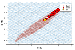
Figure 1: Subset of identified sets for Experiment 1

(a) Case 1: $\left(\theta^{RS},\theta^{RN}\right)$

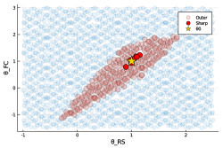
(b) Case 2: $\left(\theta^{RS},\theta^{FC}\right)$

  

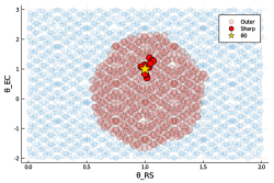
(c) Case 3: $\left(\theta^{RS},\theta^{EC}\right)$

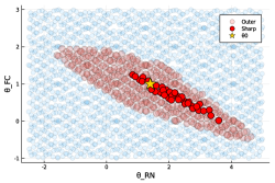
(d) Case 4: $\left(\theta^{RN},\text{$\theta^{FC}$}\right)$

  

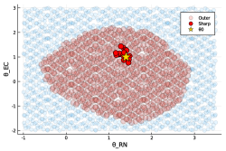
(e) Case 5: $\left(\theta^{RN},\theta^{EC}\right)$

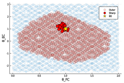
(f) Case 6: $\left(\theta^{FC},\theta^{EC}\right)$

In Figure 1, we show two identified sets. The “sharp” set corresponds to $\Theta_{I}^{MCE}\left(S^{\varepsilon_{i}}\right)$ and the “outer” set corresponds to $\Theta_{I}^{MCE}\left(S^{null}\right)$. Recall that $\Theta_{I}^{MCE}\left(S^{\varepsilon_{i}}\right)\subseteq\Theta_{I}^{MCE}\left(S^{null}\right)$, but computing $\Theta_{I}^{MCE}\left(S^{null}\right)$ is easier since determining $\theta\in\Theta_{I}^{MCE}\left(S^{null}\right)$ amounts to solving a linear program. The figure demonstrates that $\Theta_{I}^{MCE}\left(S^{null}\right)$ is helpful in ruling out points that are not the members of the identified set of interest.

5.2 Experiment 2

In this example, there are $I=2$ players whose per-period payoffs are given as

$$u_{i}\left(a_{i,t},a_{-i,t},z_{i,t},w_{i},\varepsilon_{i,t}\right)=\begin{cases}\theta^{m}+\theta^{c}a_{-i,t}+\theta^{e}\left(1-z_{i,t}\right)+\theta^{w}w_{i}+\varepsilon_{i,t}&\text{if }a_{i,t}=1\\ \theta^{\kappa}z_{i,t}&\text{if }a_{i,t}=0\end{cases}$$

where $a_{i,t}\in\mathcal{A}_{i}=\left\{0,1\right\}$ is the entry decision, $z_{i,t}\in\mathcal{Z}_{i}=\left\{0,1\right\}$ denotes the incumbency status, and $w_{i}\in\mathcal{W}_{i}\subseteq\mathbb{R}$ is player-specific and time-invariant. Each shock $\varepsilon_{i,t}$ independently follows the standard normal distribution. There are five parameters $\theta=\left(\theta^{m},\theta^{c},\theta^{e},\theta^{w},\theta^{\kappa}\right)$; $\theta^{m}$ is the monopoly profit; $\theta^{c}$ is the competition effect; $\theta^{e}$ is the entry cost; $\theta^{w}$ is the parameter associated with the excluded variables; $\theta^{\kappa}$ is the scrap value.

We set $\delta=0.9$ and $\theta_{0}=\left(\theta_{0}^{m},\theta_{0}^{c},\theta_{0}^{e},\theta_{0}^{w},\theta_{0}^{\kappa}\right)=\left(1.2,-0.8,-0.5,1.0,0.3\right)$. We generate conditional choice probabilities from a Markov perfect equilibrium that maximizes the probability that both players are active. We consider two sets of excluded covariates: $\mathcal{W}_{i}^{0}=\left\{-0.5,0.5\right\}$ and $\mathcal{W}_{i}^{1}=\left\{-1.0,1.0\right\}$. Following Pesendorfer and Schmidt-Dengler (2008), we assume $\theta_{0}^{\kappa}$ is known.

Table 2: Projection of Identified Set

				True value	$\mathcal{W}_{i}^{0}$	$\mathcal{W}_{i}^{1}$
			$\theta^{m}$	$1.2$	$\left[-1.91,3.37\right]$	$\left[0.73,2.31\right]$
			$\theta^{c}$	$-0.8$	$\left[-4.10,3.49\right]$	$\left[-2.15,-0.34\right]$
			$\theta^{e}$	$-0.5$	$\left[-0.77,0.17\right]$	$\left[-0.75,-0.09\right]$
			$\theta^{w}$	$1.0$	$\left[0.40,1.51\right]$	$\left[0.73,1.15\right]$

• Notes: The table reports the MCE identified sets under $S^{\varepsilon_{i}}$.

Table 2 shows that, as seen illustrated by Magnolfi and Roncoroni (2022) in the static case, larger variations in excluded covariates contribute to shrinkage in the identified set.

6 Conclusion

In this paper, we have studied informationally robust econometric analysis in a class of dynamic Markov games. We have introduced Markov correlated equilibrium and showed that it allows tractable characterization of Markov perfect equilibrium predictions when the underlying information structure is unknown to the analyst. We have also proposed computational strategies for obtaining the identified sets.

Several tasks remain for future research. First, it is important to introduce computationally light approaches that will work well for problems of realistic size so that the proposed framework can be readily applied for various empirical works. Second, it is also important to propose tractable strategies for constructing the confidence set. We plan to introduce computationally attractive strategies for estimation and inference based on convexification of non-convex programs and consider empirical applications to illustrate the usefulness of the framework.

Appendix

Appendix A Proofs

A.1 Proof of Lemma 1

$\left(\Rightarrow\right)$ Let $\beta$ be a MPE of $\left(G,S\right)$. $\beta$ induces $\left(G^{\beta},S\right)$. The BNE best-response condition is directly implied by the MPE condition of $\left(G,S\right)$.

$\left(\Leftarrow\right)$ Let $\beta$ be a BNE of $\left(G^{\beta},S\right)$. The BNE best-response condition implies that there is no profitable one-shot deviation given that each player expects all players to follow the prescription of $\beta$ in the future. The absence of profitable one-shot deviation implies that $\beta$ is a subgame perfect equilibrium of $\left(G,S\right)$ by the one-shot deviation principle. Therefore, $\beta$ is a MPE of $\left(G,S\right)$. $\square$

A.2 Proof of Lemma 2

Proven in the main text. $\square$

A.3 Proof of Lemma 3

It is enough to show that $V_{i}^{\beta}\left(x\right)=V_{i}^{\sigma}\left(x\right)$ for all $i\in\mathcal{I}$ and $x\in\mathcal{X}$ because then it follows that $v_{i}^{\beta}\left(a,x,\varepsilon\right)=v_{i}^{\sigma}\left(a,x,\varepsilon\right)$ for all $i\in\mathcal{I}$, $a\in\mathcal{A}$, $x\in\mathcal{X}$, and $\varepsilon\in\mathcal{E}$.

Recall that $V_{i}^{\beta}$ and $V_{i}^{\sigma}$ satisfies

$$V_{i}^{\beta}\left(x\right) =\sum_{\varepsilon,\tau,\tilde{\tau},a}\psi_{\varepsilon|x}\pi_{\tau|x,\varepsilon}\lambda_{\tilde{\tau}|x,\varepsilon,\tau}\beta_{a|x,\tau,\tilde{\tau}}\left(u_{i}\left(a,x,\varepsilon\right)+\delta\sum_{x^{\prime}}V_{i}^{\beta}\left(x^{\prime}\right)f_{x^{\prime}|a,x,\varepsilon}\right)$$

$$V_{i}^{\sigma}\left(x\right) =\sum_{\varepsilon,\tau,a}\psi_{\varepsilon|x}\pi_{\tau|x,\varepsilon}\sigma_{a|x,\varepsilon,\tau}\left(u_{i}\left(a,x,\varepsilon\right)+\delta\sum_{x^{\prime}}V_{i}^{\sigma}\left(x^{\prime}\right)f_{x^{\prime}|a,x,\varepsilon}\right)$$

for all $x\in\mathcal{X}$, where $\beta_{a|x,\tau,\tilde{\tau}}\equiv\prod_{j=1}^{I}\beta_{j}\left(a_{j}|x,\tau_{j},\tilde{\tau}_{j}\right)$. But since $\beta$ induces $\sigma$,

$$V_{i}^{\beta}\left(x\right) =\sum_{\varepsilon,\tau,a}\psi_{\varepsilon|x}\pi_{\tau|x,\varepsilon}\left(\sum_{\tilde{\tau}}\lambda_{\tilde{\tau}|x,\varepsilon,\tau}\beta_{a|x,\tau,\tilde{\tau}}\right)\left(u_{i}\left(a,x,\varepsilon\right)+\delta\sum_{x^{\prime}}V_{i}^{\beta}\left(x^{\prime}\right)f_{x^{\prime}|a,x,\varepsilon}\right)$$

$$=\sum_{\varepsilon,\tau,a}\psi_{\varepsilon|x}\pi_{\tau|x,\varepsilon}\sigma_{a|x,\varepsilon,\tau}\left(u_{i}\left(a,x,\varepsilon\right)+\delta\sum_{x^{\prime}}V_{i}^{\beta}\left(x^{\prime}\right)f_{x^{\prime}|a,x,\varepsilon}\right).$$

Comparison of the equations defining $V_{i}^{\beta}$ and $V_{i}^{\sigma}$ implies that $V_{i}^{\beta}=V_{i}^{\sigma}$, which is what we wanted to show. $\square$

A.4 Proof of Theorem 1

To prove the statement of the theorem, we make use of Theorem 1 of BM, which we restate below.

Lemma 4 (BM Theorem 1).

A decision rule $\sigma$ is a Bayes correlated equilibrium of $\left(G,S\right)$ if and only if, for some expansion $S^{*}$ of $S$, there is a Bayes Nash equilibrium of $\left(G,S^{*}\right)$ that induces $\sigma$.

$\left(\subseteq\right)$ Suppose $\sigma$ is a MCE of $\left(G,S\right)$. We want to show that there exists an expansion $S^{*}$ and a strategy profile $\beta$ in $\left(G,S^{*}\right)$ such that $\beta$ is a MPE of $\left(G,S^{*}\right)$ and $\beta$ induces $\sigma$. Since $\sigma$ is a MCE of $\left(G,S\right)$, it is a BCE of $\left(G^{\sigma},S\right)$. By BM Theorem 1, there exists an expansion $S^{*}$ of $S$ and a strategy profile $\beta$ of $\left(G^{\sigma},S^{*}\right)$ such that $\beta$ is a BNE of $\left(G^{\sigma},S^{*}\right)$ and $\beta$ induces $\sigma$. But since $G^{\sigma}=G^{\beta}$, $\beta$ is also a BNE of $\left(G^{\beta},S^{*}\right)$, which in turn implies that $\beta$ is a MPE of $\left(G,S^{*}\right)$.

$\left(\supseteq\right)$ Suppose $\beta$ is a MPE of $\left(G,S^{*}\right)$. We want to show that if $\beta$ induces $\sigma$ in $\left(G,S\right)$, then $\sigma$ is a MCE of $\left(G,S\right)$. Since $\beta$ is a MPE of $\left(G,S^{*}\right)$, it is a BNE of $\left(G^{\beta},S^{*}\right)$. By BM Theorem 1, if $\sigma$ is induced by $\beta$, then $\sigma$ is a BCE of $\left(G^{\beta},S\right)$. But since $G^{\beta}=G^{\sigma}$, $\sigma$ is also a BCE of $\left(G^{\sigma},S\right)$, which in turn implies that $\sigma$ is a MCE of $\left(G,S\right)$. $\square$

A.5 Proof of Corollary 1

$\left(\subseteq\right)$ Take $\phi\in\mathcal{P}_{a|x}^{MCE}\left(G,S\right)$. By definition, there exists $q\in\mathcal{P}_{a|x,\varepsilon,\tau}^{MCE}\left(G,S\right)$ such that $q$ induces $\phi$, i.e.,

$$\phi_{a|x}=\sum_{\varepsilon\in\mathcal{E},\tau\in\mathcal{T}}\psi_{\varepsilon|x}\pi_{\tau|x,\varepsilon}q_{a|x,\varepsilon,\tau},\quad\forall a\in\mathcal{A},x\in\mathcal{X}.$$

Then there exists a $S^{*}$ such that $S^{*}\succsim_{E}S$ and $q\in\mathcal{P}_{a|x,\varepsilon,\tau}^{MPE}\left(G,S^{*}\right)$, implying that $\phi\in\mathcal{P}_{a|x}^{MPE}\left(G,S^{*}\right)$.

$\left(\supseteq\right)$ Take $\phi\in\bigcup_{S^{*}\succsim_{E}S}\mathcal{P}_{a|x}^{MPE}\left(G,S^{*}\right)$. Then there exists $S^{*}$ such that $S^{*}\succsim_{E}S$ and $\phi\in\mathcal{P}_{a|x}^{MPE}\left(G,S^{*}\right)$ which implies that there exists $q\in\mathcal{P}_{a|x,\varepsilon,\tau}^{MPE}\left(G,S^{*}\right)$ such that $q$ induces $\phi$. Then since $q\in\mathcal{P}_{a|x,\varepsilon,\tau}^{MCE}\left(G,S\right)$, we have $q\in\mathcal{P}_{a|x}^{MCE}\left(G,S\right)$. $\square$

A.6 Proof of Theorem 2

We want to show

$$\Theta_{I}^{MCE}\left(S\right)=\bigcup_{\tilde{S}\succsim_{E}S}\Theta_{I}^{MPE}\left(\tilde{S}\right).$$

To prove the equality, note that

$$\Theta_{I}^{MCE}\left(S\right)\equiv\left\{\theta\in\Theta:\ \phi\in\mathcal{P}_{a|x}^{MCE}\left(G^{\theta},S\right)\right\}$$

and

$$\bigcup_{\tilde{S}\succsim_{E}S}\Theta_{I}^{MPE}\left(\tilde{S}\right) \equiv\bigcup_{\tilde{S}\succsim_{E}S}\left\{\theta\in\Theta:\ \phi\in\mathcal{P}_{a|x}^{MPE}\left(G^{\theta},\tilde{S}\right)\right\}$$

$$=\bigcup_{\tilde{S}\succsim_{E}S}\left\{\theta\in\Theta:\ \phi\in\bigcup_{\tilde{S}\succsim_{E}S}\mathcal{P}_{a|x}^{MPE}\left(G^{\theta},\tilde{S}\right)\right\}.$$

But by Corollary 1, we have

$$\mathcal{P}_{a|x}^{MCE}\left(G,S\right)=\bigcup_{S^{*}\succsim_{E}S}\mathcal{P}_{a|x}^{MPE}\left(G,S^{*}\right).$$

Thus, we must have $\Theta_{I}^{MCE}\left(S\right)=\bigcup_{\tilde{S}\succsim_{E}S}\Theta_{I}^{MPE}\left(\tilde{S}\right)$. $\square$

A.7 Proof of Theorem 3

The proof is straightforward by comparing the mathematical program to the original equilibrium conditions and the definition of the identified set. $\square$

A.8 Proof of Theorem 4

To see the feasibility of the program, take any $\sigma$ such that $\sigma\in\Delta_{a|x,\varepsilon,\tau}$ and $\phi=\phi\left(\sigma\right)$. Given $\sigma$, $V$ is determined. Finally, given $\sigma$ and $V$, there must exist some $t$ that satisfies all the inequality conditions.

Next, that $Q\left(\theta\right)=0$ if and only if $\theta\in\Theta_{I}$ is trivial. $\square$

References

- Aguirregabiria et al. (2021) Aguirregabiria, V., A. Collard-Wexler, and S. P. Ryan (2021): “Dynamic games in empirical industrial organization,” in Handbook of Industrial Organization, ed. by K. Ho, A. Hortaçsu, and A. Lizzeri, Elsevier, vol. 4 of Handbook of Industrial Organization, Volume 4, 225–343.
- Aguirregabiria and Mira (2007) Aguirregabiria, V. and P. Mira (2007): “Sequential Estimation of Dynamic Discrete Games,” Econometrica, 75, 1–53.
- Aguirregabiria and Mira (2010) ——— (2010): “Dynamic discrete choice structural models: A survey,” Journal of Econometrics, 156, 38–67.
- Bajari et al. (2007) Bajari, P., C. L. Benkard, and J. Levin (2007): “Estimating Dynamic Models of Imperfect Competition,” Econometrica, 75, 1331–1370.
- Beresteanu et al. (2011) Beresteanu, A., I. Molchanov, and F. Molinari (2011): “Sharp Identification Regions in Models With Convex Moment Predictions,” Econometrica, 79, 1785–1821.
- Bergemann and Morris (2013) Bergemann, D. and S. Morris (2013): “Robust Predictions in Games With Incomplete Information,” Econometrica, 81, 1251–1308.
- Bergemann and Morris (2016) ——— (2016): “Bayes correlated equilibrium and the comparison of information structures in games,” Theoretical Economics, 11, 487–522.
- Doraszelski and Escobar (2010) Doraszelski, U. and J. F. Escobar (2010): “A theory of regular Markov perfect equilibria in dynamic stochastic games: Genericity, stability, and purification,” Theoretical Economics, 5, 369–402.
- Doval and Ely (2020) Doval, L. and J. C. Ely (2020): “Sequential Information Design,” Econometrica, 88, 2575–2608.
- Egesdal et al. (2015a) Egesdal, M., Z. Lai, and C.-L. Su (2015a): “Estimating dynamic discrete-choice games of incomplete information,” Quantitative Economics, 6, 567–597.
- Egesdal et al. (2015b) ——— (2015b): “Estimating dynamic discrete-choice games of incomplete information,” Quantitative Economics, 6, 567–597.
- Ericson and Pakes (1995) Ericson, R. and A. Pakes (1995): “Markov-Perfect Industry Dynamics: A Framework for Empirical Work,” The Review of Economic Studies, 62, 53–82.
- Fershtman and Pakes (2012) Fershtman, C. and A. Pakes (2012): “Dynamic games with asymmetric information: A framework for empirical work,” The Quarterly Journal of Economics, 127, 1611–1661.
- Fudenberg and Tirole (1991) Fudenberg, D. and J. Tirole (1991): Game Theory, vol. 1, The MIT Press.
- Gualdani and Sinha (2020) Gualdani, C. and S. Sinha (2020): “Identification and inference in discrete choice models with imperfect information,” arXiv:1911.04529 [econ], arXiv: 1911.04529.
- Kasahara and Shimotsu (2012) Kasahara, H. and K. Shimotsu (2012): “Sequential Estimation of Structural Models With a Fixed Point Constraint,” Econometrica, 80, 2303–2319.
- Kennan (2006) Kennan, J. (2006): “A Note on Discrete Approximations of Continuous Distributions,” Unpublished Manuscript. URL: https://www.ssc.wisc.edu/~jkennan/research/DiscreteApprox.pdf (Last accessed: October 2021).
- Koh (2022) Koh, P. (2022): “Stable Outcomes and Information in Games: An Empirical Framework,” Working Paper.
- Magnolfi and Roncoroni (2022) Magnolfi, L. and C. Roncoroni (2022): “Estimation of Discrete Games with Weak Assumptions on Information,” Working Paper. URL: https://static1.squarespace.com/static/5608a251e4b054aa1dda30bc/t/624631db0bfcf20cd00e5cd8/1648767452870/EstimationDiscrGamesWeakInfo_MagnolfiRoncoroni_Mar2022.pdf.
- Mailath and Samuelson (2006) Mailath, G. J. and L. Samuelson (2006): Repeated Games and Reputations: Long-Run Relationships, Oxford University Press, USA.
- Makris and Renou (2021) Makris, M. and L. Renou (2021): “Information Design in Multi-stage Games,” arXiv:2102.13482 [econ], arXiv: 2102.13482.
- Pakes et al. (2007) Pakes, A., M. Ostrovsky, and S. Berry (2007): “Simple estimators for the parameters of discrete dynamic games (with entry/exit examples),” The RAND Journal of Economics, 38, 373–399.
- Pakes et al. (2015) Pakes, A., J. Porter, K. Ho, and J. Ishii (2015): “Moment Inequalities and Their Application,” Econometrica, 83, 315–334.
- Pesendorfer and Schmidt-Dengler (2008) Pesendorfer, M. and P. Schmidt-Dengler (2008): “Asymptotic Least Squares Estimators for Dynamic Games,” The Review of Economic Studies, 75, 901–928.
- Rust (1994) Rust, J. (1994): “Estimation of dynamic structural models, problems and prospects: discrete decision processes,” in Advances in Econometrics: Sixth World Congress, ed. by C. A. Sims, Cambridge: Cambridge University Press, vol. 2 of Econometric Society Monographs, 119–170.
- Su and Judd (2012) Su, C.-L. and K. L. Judd (2012): “Constrained Optimization Approaches to Estimation of Structural Models,” Econometrica, 80, 2213–2230.
- Syrgkanis et al. (2021) Syrgkanis, V., E. Tamer, and J. Ziani (2021): “Inference on Auctions with Weak Assumptions on Information,” Working Paper. URL: https://scholar.harvard.edu/files/tamer/files/bce_econometrics.pdf.