Gravitational waveforms from the inspiral of compact binaries in the Brans-Dicke theory in an expanding Universe

Abstract

In modified gravity theories, such as the Brans-Dicke theory, the background evolution of the Universe and the perturbation around it are different from that in general relativity. Therefore, the gravitational waveforms used to study standard sirens in these theories should be modified. The modifications of the waveforms can be classified into two categories: wave generation effects and wave propagation effects. Hitherto, the waveforms used to study standard sirens in the modified gravity theories incorporate only the wave propagation effects and ignore the wave generation effects; while the waveforms focusing on the wave generation effects, such as the post-Newtonian waveforms, do not incorporate the wave propagation effects and cannot be directly applied to the sources with non-negligible redshifts in the study of standard sirens. In this work, we construct the consistent waveforms for standard sirens in the Brans-Dicke theory. The wave generation effects include the emission of the scalar breathing polarization $h_{b}$ and the corrections to the tensor polarizations $h_{+}$ and $h_{\times}$; the wave propagation effect is the modification of the luminosity distance for the gravitational waveforms. Using the consistent waveforms, we analyze the parameter estimation biases due to the ignorance of the wave generation effects. Considering the observations by the Einstein Telescope, we find that the ratio of the theoretical bias to the statistical error of the redshifted chirp mass is two orders of magnitude larger than that of the source distance. For black hole-neutron star binary systems like GW191219, the theoretical bias of the redshifted chirp mass can be several times larger than the statistical error.

I Introduction

The Hubble constant describes the present expansion rate of the Universe Mukhanov (2005). The recent local measurement of the Hubble constant from the Ia supernovae explosions is a factor of 9% larger than the large scale measurement from the cosmic microwave background data. This discrepancy is $5\sigma$ and is called the Hubble tension Riess et al. . In addition to these methods, gravitational waves (GWs) can be used to determine the Hubble constant. Since the GWs emitted by the compact binaries are well modeled and the measured waveforms can be used to determine their cosmological distances. Such binaries are called standard sirens Schutz (1986); Holz and Hughes (2005) which are the GW analog with electromagnetic standard candles. Combined with the redshift of the GW sources, the Hubble constant can be measured by the observation of the standard sirens. The detection of the binary neutron star merger event GW170817 in both GWs and electromagnetic waves is the first realization of the measurement of the Hubble constant by the standard siren Abbott et al. (2017). Standard sirens can provide new insight into the solution of the Hubble tension Chen (2020). For a review of the standard sirens, please see Zhao (2018).

The Hubble tension can also be solved by the modified gravity theories Valentino et al. (2021). It has been shown that the tension between the local and large scale measurement of the Hubble constant can be smoothed out if the observational data are interpreted in the Brans-Dicke theory rather than in general relativity (GR) Solà Peracaula et al. (2019). The Brans-Dicke theory is a scalar-tensor theory which is an extension of GR with a massless scalar field Brans and Dicke (1961); *Dicke1959; *Dicke1962. A large and growing body of literature has investigated GWs in scalar-tensor theories Cao et al. (2021); Hou and Zhu (2021); Tahura et al. (2021); Cao et al. (2013); Maselli et al. (2022); Liu et al. (2020); Higashino and Tsujikawa . The gravitational waveforms emitted by inspiralling compact binaries have been calculated systematically using the post-Newtonian (PN) method Oliynyk (2009); Poisson and Will (2014) when the gravitational fields are weak and the orbital velocities are small. The leading order Newtonian quadrupole waveforms have been obtained in Will (1994). Then, the higher PN order contributions to the waveforms were calculated in different approaches Mirshekari and Will (2013); Lang (2014, 2015); Sennett et al. (2016); Bernard et al. . In these PN waveforms, the binary system is modeled as two point particles moving along circular orbits. In recent years, the eccentricity of the orbit Ma and Yunes (2019), the spins of the components Kopeikin (2020); Brax et al. (2021), and the tidal interaction between the components Bernard (2020) have been incorporated into the waveforms. However, these waveforms and other waveforms focusing on wave generation effects Maselli et al. (2022); Barausse et al. (2013); Yunes et al. (2012) cannot be used to study standard sirens in cosmological distances with non-negligible redshifts because they are calculated on the Minkowski background.

Focusing on the Brans-Dicke theory as an example, the present work serves as a first step to coherently construct gravitational waveforms from compact binaries in the expanding Universe in the modified gravity theories. Compared with GR, the modified gravity theories can predict different expansion history of the background Friedmann-Lemaître-Robertson-Walker (FLRW) universe Clifton et al. (2012) and change the gravitational waveforms which are perturbations around the background Barack et al. (2019). The modifications of the waveforms can be classified into two categories: wave generation effects Tahura and Yagi (2018); *PhysRevD.101.109902 and wave propagation effects Nishizawa (2018); *PhysRevD.97.104038; *PhysRevD.99.104038. It is well known that GWs have two tensor polarizations ($h_{+}$ and $h_{\times}$) in GR Misner et al. (1973). During wave generation, the modified gravity can induce extra polarization(s) as well as amplitude and phase corrections to the tensor polarizations Tahura and Yagi (2018); *PhysRevD.101.109902. When the waves propagate through the Universe, the modified gravity can also produce amplitude and phase correction to the tensor polarizations Nishizawa (2018); *PhysRevD.97.104038; *PhysRevD.99.104038; Zhao et al. (2020). However, all previous studies on the standard sirens in the modified gravity have ignored the wave generation effects and used inconsistent gravitational waveforms Lagos et al. (2019); Dalang et al. (2020, 2021); Baker and Harrison (2021); Belgacem et al. (2019a); Dalang and Lombriser (2019); Belgacem et al. (2018a); D’Agostino and Nunes (2019); Wolf and Lagos (2020); Belgacem et al. (2019b); Matos et al. (2021); Amendola et al. (2018). For instance, see Eq. (14) in Lagos et al. (2019) and Eq. (12) in Matos et al. (2021).

To construct consistent waveforms which consider both the wave generation and wave propagation effects, we follow Thorne’s suggestion Thorne (1987, 1980) that divides the wave zone where the waves propagate into local wave zone and distant wave zone. The local wave zone is near the GW source and the effect of the background curvature of the universe is negligible. Thus, the background spacetime can be seen as flat in the local wave zone and the PN method can be used to solve the field equations to obtain the GW waveforms. Then, using the geometric optics approximation Isaacson (1968a, b); Dalang et al. (2020, 2021); Kubota et al. ; Garoffolo et al. (2020), the waveforms in the local wave zone propagate into the distant wave zone in which the curvature of the universe is important. In this way, the waveforms in the distant wave zone contain both wave generation and wave propagation effects.

In this paper, we construct the consistent waveforms on the background of an expanding Universe in the Brans-Dicke theory based on the Newtonian quadrupole waveforms Will (1994); Liu et al. (2020). In particular, we obtain the time domain waveforms of two tensor polarizations and one scalar polarization (breathing polarization $h_{b}$) in the distant wave zone (cf. Eqs. (67)-(73)). We incorporate the modifications that originate from both wave generation and propagation. These waveforms are new results. As mentioned above, the wave generation effects include amplitude correction, phase correction, and additional polarization to the ones in GR; but in the Brans-Dicke theory, during wave propagation, there is only amplitude correction, and this amplitude correction appears as a modification of the electromagnetic luminosity distance. The modification of the luminosity distance in the tensor polarizations is consistent with previous studies Lagos et al. (2019); Dalang et al. (2020, 2021); Baker and Harrison (2021); Belgacem et al. (2019a); Dalang and Lombriser (2019); Belgacem et al. (2018a); D’Agostino and Nunes (2019); Wolf and Lagos (2020); Belgacem et al. (2019b); Matos et al. (2021); Amendola et al. (2018); Belgacem et al. (2018b), while the modification of the luminosity distance in the breathing polarization is a new result. Furthermore, we analyze the parameter estimation biases due to the inconsistent waveforms which ignore the wave generation effects. Considering the observation of the GWs from the black hole-neutron star (BH-NS) binaries by Einstein Telescope Punturo et al. (2010) and setting the source parameters to be that of the BH-NS candidates detected by LIGO/Virgo The LIGO Scientific Collaboration et al. , we find that the inconsistent waveforms can bias the redshifted chirp mass significantly while have negligible influence on the measurement of the distance when the Brans-Dicke coupling constant saturates the bound imposed by the Cassini spacecraft Alsing et al. (2012). For BH-NS systems like GW191219, the theoretical bias of the redshifted chirp mass can be several times larger than the statistical error.

The paper is organized as follows. In section II, we review the PN waveforms in the local wave zone in the Brans-Dicke theory. In section III, we construct the geometric optics equations for wave propagation in curved background spacetime in the Brans-Dicke theory. In section IV, we apply the geometric optics approximation to propagate the waves through the FLRW universe and obtain the waveforms in the distant wave zone. In section V, we estimate the theoretical bias due to the inconsistent waveforms. In section VI, we summarize the results and discuss the prospects for future research.

For the metric, Riemann, and Ricci tensors, we follow the conventions of Misner, Thorne, and Wheeler Misner et al. (1973). We adopt the unit $c=1$, with $c$ being the speed of light. We do not set the gravitational constant $G$ equal to 1, since the effective gravitational constant will vary over the history of the universe in this theory.

II Gravitational waveforms in the local wave zone

The space around the GW source can be divided into three regions by two length scales $r_{\text{I}}$ and $r_{\text{O}}$: a near zone $(r\lesssim r_{\text{I}})$, a local wave zone $(r_{\text{I}}\lesssim r\lesssim r_{\text{O}})$, and a distant wave zone $(r\gtrsim r_{\text{O}})$. The inner boundary of the local wave zone $r_{\rm I}$ is much larger than the GW wavelength so that the source’s gravity is weak in this region. The outer boundary of the local wave zone $r_{\rm O}$ is large enough that this region contains many wavelengths; but not so large that the background curvature of the universe influences the propagation of the GWs. Therefore, the GWs can be regarded as propagating in flat spacetime in the local wave zone. This zone is the matching region for the problem of wave generation and wave propagation .

In this section, we review the wave generation problem and present the tensor and scalar waveforms in the local wave zone. Detailed derivation can be found in Will (1994); Liu et al. (2020). The action of the Brans-Dicke theory is Alsing et al. (2012)

$$S=\frac{1}{16\pi}\int d^{4}x\sqrt{-g}\left[\phi R-\frac{\omega(\phi)}{\phi}\partial_{\mu}\phi\partial^{\mu}\phi+M\right]+S_{m}\left[g_{\mu\nu},\Psi_{m}\right],$$ (1)

where $g\equiv\det g_{\mu\nu}$ and $\omega(\phi)$ is the coupling function Damour and Esposito-Farèse (1993). The constant $M$ is associated with the effective cosmological constant and $\Psi_{m}$ denotes the matter fields collectively. The field equations are Alsing et al. (2012)

$$R_{\mu\nu}-\frac{1}{2}g_{\mu\nu}R-\frac{1}{2}\frac{M}{\phi}g_{\mu\nu}=\frac{8\pi}{\phi}T_{\mu\nu}+\frac{\omega(\phi)}{\phi^{2}}(\phi_{,\mu}\phi_{,\nu}-\frac{1}{2}g_{\mu\nu}\phi_{,\alpha}\phi^{,\alpha})+\frac{1}{\phi}(\nabla_{\mu}\nabla_{\nu}-g_{\mu\nu}\square)\phi$$ (2)

$$\square\phi-\frac{2M}{2\omega(\phi)+3}=\frac{8\pi}{2\omega(\phi)+3}(T-2\phi~{}T^{\prime})-\frac{\omega^{\prime}}{2\omega(\phi)+3}\phi_{,\alpha}\phi^{,\alpha}$$ (3)

where ${}^{\prime}\equiv\frac{d}{d\phi}$, the commas denote partial derivative, and $\square\equiv\nabla_{\nu}\nabla^{\nu}$. The covariant derivative $\nabla_{\nu}$ satisfies $\nabla_{\nu}g_{\alpha\beta}=0$. $T_{\mu\nu}$ is the stress-energy tensor of matter and $T=g^{\mu\nu}T_{\mu\nu}$.

In order to solve the wave generation problem inside the outer radius $(r\lesssim r_{\text{O}})$, the field equations should be expanded around the Minkowski background $\eta_{\mu\nu}dx^{\mu}dx^{\nu}=-dt^{2}+dr^{2}+r^{2}(d\iota^{2}+\sin^{2}\iota~{}d\sigma^{2})$ and the scalar background $\bar{\phi}$,

$$\phi=\bar{\phi}+\varphi,\qquad g_{\mu\nu}=\eta_{\mu\nu}+h_{\mu\nu},$$ (4)

$$\theta_{\mu\nu}\equiv h_{\mu\nu}-\frac{1}{2}h\eta_{\mu\nu}-\frac{\varphi}{\bar{\phi}}\eta_{\mu\nu},$$ (5)

where $|h_{\mu\nu}|\ll 1$ and $|\varphi/\bar{\phi}|\ll 1$. When we deal with the wave generation problem, the scalar background $\bar{\phi}$ can be viewed as a constant, although it will evolve with the expansion of the Universe. Imposing the harmonic gauge

$$\theta^{\mu\nu}_{\phantom{12},\mu}=0,$$ (6)

the field equations become

$$\square_{\eta}\theta_{\mu\nu}=-16\pi G\tau_{\mu\nu},$$ (7)

$$\square_{\eta}\varphi=-16\pi\mathbb{S},$$ (8)

where $\square_{\eta}=\eta^{\mu\nu}\partial_{\mu}\partial_{\nu}$ and $\tau_{\mu\nu}=T_{\mu\nu}+t_{\mu\nu}$. The source term $t_{\mu\nu}$ denotes the nonlinear perturbations collectively. The effective gravitational constant is

$$G\equiv\frac{1}{\bar{\phi}}.$$ (9)

The cosmological constant is discarded when dealing with the wave generation. For the explicit expression of the source $\mathbb{S}$ of the scalar wave equation, see Eq. (18) in Liu et al. (2020).

Consider the waves emitted by a binary system on a quasicircular orbit with orbital frequency $\omega_{e}$. When the velocity of the binary system is slow and the gravitational field is weak, the above wave equations can be solved by the PN method. The waveforms emitted by the binary system will depend on the sensitivities of the binary bodies, defined by

$$s_{A}\equiv\frac{d\ln m_{A}(\phi)}{d\ln\phi}\Big{|}_{\bar{\phi}}.$$ (10)

Since the scalar field can influence the gravitational binding energy of the compact object, the inertial mass $m_{A}(\phi)$ of object $A$ is a function of the scalar field Eardley (1975). The sensitivity of a black hole is $\frac{1}{2}$ Eardley (1975) and the typical value of the sensitivity of a neutron star is about $0.2\sim 0.3$ Zaglauer (1992); Alsing et al. (2012).

The tensor waves emitted by this binary system are given by Liu et al. (2020)

$$\theta^{\rm TT}_{\mu\nu}=h_{+}e^{+}_{\mu\nu}+h_{\times}e^{\times}_{\mu\nu},$$ (11)

where ‘TT’ denotes the transverse and traceless part. In the local wave zone, the waveforms of the two tensor polarizations at the Newtonian quadrupole order are

$$h_{+}=-4\frac{(GM_{c})^{5/3}}{r}(\tilde{g}\omega_{e})^{2/3}\frac{1+\cos^{2}\iota}{2}\cos\psi\Big{|}_{t_{r}},$$ (12)

$$h_{\times}=-4\frac{(GM_{c})^{5/3}}{r}(\tilde{g}\omega_{e})^{2/3}\cos\iota~{}\sin\psi\Big{|}_{t_{r}},$$ (13)

where the chirp mass $M_{c}$ is given by

$$M_{c}\equiv\mu^{3/5}m^{2/5}$$ (14)

with $m=m_{1}+m_{2}$, $\mu=m_{1}m_{2}/m$, and $m_{A}=m_{A}(\bar{\phi})$.

$$\tilde{g}\equiv 1+\alpha(1-2s_{1})(1-2s_{2}),\qquad\alpha\equiv\frac{1}{2\omega(\bar{\phi})+3}.$$ (15)

The factor $\tilde{g}$ originates from the modification of Kepler’s law Liu et al. (2020).

The coordinates are adapted so that the binary system is at the origin $r=0$ and $\iota$ is the angle between the line of sight and the angular momentum of the binary system. The phase of the tensor wave is given by

$$\psi(t_{r})=2\int^{t_{r}}\omega_{e}(t^{\prime})dt^{\prime},$$ (16)

where $\omega_{e}(t)$ is the orbital frequency of binary system at time $t$ and the retarded time is

$$t_{r}=t-r.$$ (17)

In the local wave zone, the polarization tensors are

$$e^{\mu\nu}_{+}=e_{(\iota)}^{\mu}e_{(\iota)}^{\nu}-e_{(\sigma)}^{\mu}e_{(\sigma)}^{\nu},\qquad e^{\mu\nu}_{\times}=e_{(\iota)}^{\mu}e_{(\sigma)}^{\nu}+e_{(\sigma)}^{\mu}e_{(\iota)}^{\nu},$$ (18)

where

$$e_{(\iota)}=\frac{1}{r}\frac{\partial}{\partial\iota},\qquad e_{(\sigma)}=\frac{1}{r\sin\iota}\frac{\partial}{\partial\sigma}.$$ (19)

In the local wave zone, the waveforms of the scalar wave to the Newtonian quadruple order are

$$\varphi=\phi_{1}+\phi_{2},$$ (20)

where

$$\phi_{1}=-2\alpha~{}\frac{\mu}{r}~{}2\mathcal{S}(G\tilde{g}m\omega_{e})^{1/3}\sin\iota\cos(\frac{1}{2}\psi)\Big{|}_{t_{r}},$$ (21)

$$\phi_{2}=2\alpha~{}\frac{\mu}{r}~{}\Gamma(G\tilde{g}m\omega_{e})^{2/3}\sin^{2}\iota\cos(\psi)\Big{|}_{t_{r}},$$ (22)

with

$$\begin{split}\mathcal{S}&\equiv s_{1}-s_{2},\\ \Gamma&\equiv\frac{(1-2s_{1})m_{2}+(1-2s_{2})m_{1}}{m}.\end{split}$$ (23)

$\phi_{1}$ and $\phi_{2}$ represent the scalar dipole and quadrupole radiation, respectively.

Scalar and tensor waves will carry away the orbital energy of the binary system, and the orbital frequency will increase with time. Using the PN method, the time derivative of the orbital frequency has been obtained Will (1994); Liu et al. (2020)

$$\frac{d\omega_{e}}{dt_{r}}=\frac{96}{5}K(GM_{c})^{\frac{5}{3}}\omega_{e}^{\frac{11}{3}}+K_{1}G\mu\omega_{e}^{3}$$ (24)

with

$$K\equiv\tilde{g}^{\frac{2}{3}}(1+\frac{1}{6}\alpha\Gamma^{2}),\qquad K_{1}\equiv 4\alpha\mathcal{S}^{2}.$$ (25)

The evolution of the phase $\psi$ can be obtained by using the above equations.

III Wave propagation and geometric optics approximation

The last section has solved the wave generation problem inside the outer radius $(r\lesssim r_{\rm O})$. This section will establish the equations governing the wave propagation outside the inner radius $(r\gtrsim r_{\rm I})$. In this region, the tensor and scalar waves can be seen as small ripples in a curved, slowly changing background. The frequency of the ripples is high compared to the time scale of background changes, but their amplitudes are small. Therefore, outside the inner radius, tensor and scalar waves can be viewed as linear perturbations around the background and the high frequency approximation, i.e., geometric optics approximation, can be used to solve the perturbation equations.

III.1 Linear perturbations

Consider the perturbations over an arbitrary background,

$$g_{\mu\nu}=\bar{g}_{\mu\nu}+h_{\mu\nu},\qquad\phi=\bar{\phi}+\varphi.$$ (26)

The overhead bar denotes the background quantity. Let us study the perturbations $h_{\mu\nu}$ and $\varphi$ via the field equations (2) and (3) linearized about the background $\bar{g}_{\mu\nu}$ and $\bar{\phi}$. Note that the scalar background $\bar{\phi}$ is viewed as a constant when dealing with the wave generation in the previous section. But it can evolve in space and time when we consider the wave propagation problem on much larger scales.

From the field equations (2) and (3), the linear perturbation equations are

$$\begin{split}&\bar{\phi}(-\frac{1}{2}\bar{\square}\hat{h}_{\mu\nu}+\tensor{\hat{h}}{{}_{\beta(\mu|}^{\beta}{}_{\nu}{}_{)}}-\frac{1}{2}\bar{g}_{\mu\nu}\tensor{\hat{h}}{{}_{\alpha\beta|}^{\alpha\beta}})-\bar{\nabla}_{\mu}\bar{\nabla}_{\nu}\varphi+\bar{g}_{\mu\nu}\bar{\square}\varphi-\bar{F}(2\bar{\phi}_{|(\mu}\varphi_{|\nu)}-\bar{g}_{\mu\nu}\bar{\phi}^{|\alpha}\varphi_{|\alpha})\\ &+\frac{1}{2}\bar{\phi}^{|\beta}(2\hat{h}_{\beta(\mu|\nu)}-\hat{h}_{\mu\nu|\beta}-2\bar{g}_{\mu\nu}\tensor{\hat{h}}{{}_{\beta\rho|}^{\rho}}-\bar{g}_{\beta(\mu}\hat{h}_{|\nu)}+\frac{1}{2}\bar{g}_{\mu\nu}\hat{h}_{|\beta})=0,\end{split}$$ (27)

$$\bar{\square}\varphi-(\frac{1}{\bar{\phi}}-\frac{2\bar{\omega}^{\prime}}{2\bar{\omega}+3})\bar{\phi}_{|\alpha}\varphi^{|\alpha}=0.$$ (28)

Here $\bar{\nabla}_{\mu}$ and the slash $|$ denote the covariant derivative such that $\bar{\nabla}_{\mu}\bar{g}_{\alpha\beta}=\bar{g}_{\alpha\beta|\mu}=0$ and $\bar{\square}\equiv\bar{\nabla}_{\mu}\bar{\nabla}^{\mu}$. The background metric $\bar{g}^{\mu\nu}$ is used to raise the indices. The hat indicates the trace-reversed part of a tensor, e.g., $\hat{h}_{\mu\nu}=h_{\mu\nu}-\frac{1}{2}\bar{g}^{\mu\nu}\bar{g}^{\alpha\beta}h_{\alpha\beta}$ and $\hat{h}=\bar{g}^{\alpha\beta}\hat{h}_{\alpha\beta}$. The function $F$ is given by $F\equiv\frac{\omega(\phi)}{\phi}$. Indices placed between round brackets are symmetrized, e.g., $\hat{h}_{\beta(\mu|\nu)}=\frac{1}{2}(\hat{h}_{\beta\mu|\nu}+\hat{h}_{\beta\nu|\mu})$.

Note that terms that do not contain derivatives with respect to the perturbation fields are discarded. Since we focus on the high frequency wave solutions of the perturbations, a term is larger when it contains more derivatives. It will be shown in the following subsection that the above perturbation equations are adequate for the accuracy required in this paper. Because the interaction between matter and GWs is weak, the perturbation of the stress-energy tensor $\delta T_{\mu\nu}$ induced by GWs is also ignored Thorne (1983). The tensor perturbation equation (LABEL:tp) is consistent with Eqs. (A9)-(A14) and (A21)-(A27) in Dalang et al. (2021). The scalar perturbation equation (28) is consistent with Eqs. (A50)-(A53) and (A57)-(A64) in Dalang et al. (2021).

The second derivatives of $\varphi$ in the tensor perturbation equation (LABEL:tp) can be eliminated by introducing the eigentensor perturbation Dalang et al. (2021)

$$\theta_{\mu\nu}=\hat{h}_{\mu\nu}-\bar{g}_{\mu\nu}\frac{\varphi}{\bar{\phi}}.$$ (29)

Imposing the harmonic gauge

$$\tensor{\theta}{{}_{\mu\nu|}^{\mu}}=0,$$ (30)

the tensor perturbation equation (LABEL:tp) is further simplified to

$$\begin{split}&-\frac{1}{2}\bar{\phi}~{}\bar{\square}\theta_{\mu\nu}+\frac{1}{2}\bar{\phi}^{|\beta}(\theta_{\beta\mu|\nu}+\theta_{\beta\nu|\mu}-\theta_{\mu\nu|\beta})-\frac{1}{4}(\bar{\phi}_{|\mu}\theta_{|\nu}+\bar{\phi}_{|\nu}\theta_{|\mu}-\bar{g}_{\mu\nu}\theta_{|\beta}\bar{\phi}^{|\beta})\\ &-(\frac{3}{2\bar{\phi}}+\bar{F})(\bar{\phi}_{|\mu}\varphi_{|\nu}+\bar{\phi}_{|\nu}\varphi_{|\mu}-\bar{g}_{\mu\nu}\varphi_{|\beta}\bar{\phi}^{|\beta})=0,\end{split}$$ (31)

where $\theta\equiv\bar{g}^{\mu\nu}\theta_{\mu\nu}$. The above equation is consistent with Eqs. (A54)-(A56), (A65)-(A67), and (A73)-(A74) in Dalang et al. (2021) .

III.2 Geometric optics approximation

Now we consider the high frequency wave ansatz

$$\varphi=\Re[\Phi e^{iv}],\qquad\theta_{\mu\nu}=\Re[\Theta_{\mu\nu}e^{i\psi}]$$ (32)

of the perturbation equations (28) and (LABEL:tp2). Here $\Phi$ and $\Theta_{\mu\nu}$ denote the complex amplitudes of the waves, and $v$ and $\psi$ are their phases. $\Re$ denotes the real part of the argument. Since the waves satisfy the geometric optics approximation outside the inner radius, their phases vary much more rapidly than their amplitudes and the background fields,

$$\partial v,~{}\partial\psi\gg\partial\ln|\Phi|,~{}\partial\ln|\Theta_{\mu\nu}|,~{}\partial\ln|\bar{\phi}|,~{}\partial\ln|\bar{g}_{\mu\nu}|.$$ (33)

Therefore, the terms in the perturbation equations can be sorted according to their power of the wave vectors

$$q_{\alpha}\equiv-\partial_{\alpha}v,\qquad k_{\alpha}\equiv-\partial_{\alpha}\psi.$$ (34)

Note that, for both the tensor and scalar waves, we consider only one frequency component in this section, although there are multiple frequency components in realistic situations (cf. Eq. (20)). Because different frequency components are uncoupled during propagation, they can be treated separately Dalang et al. (2021). It can also be seen from Eq. (20) that the phase $v$ of the scalar wave is proportional to the phase $\psi$ of the tensor wave. Consequently, $q_{\alpha}$ and $k_{\alpha}$ are in parallel.

Substituting the wave ansatz (32) into Eq. (LABEL:tp2) yields

$$\begin{split}&-\frac{1}{2}\bar{\phi}[-k^{\alpha}k_{\alpha}\Theta_{\mu\nu}-2ik_{\alpha}\bar{\nabla}^{\alpha}\Theta_{\mu\nu}-i\bar{\nabla}^{\alpha}k_{\alpha}\Theta_{\mu\nu}]e^{i\psi}+\frac{1}{2}\bar{\phi}^{|\beta}[-ik_{\nu}\Theta_{\beta\mu}-ik_{\mu}\Theta_{\beta\nu}+ik_{\beta}\Theta_{\mu\nu}]e^{i\psi}\\ &-\frac{1}{4}[-ik_{\nu}\bar{\phi}_{|\mu}-ik_{\mu}\bar{\phi}_{|\nu}+i\bar{g}_{\mu\nu}k_{\beta}\bar{\phi}^{|\beta}]\Theta e^{i\psi}+(\frac{3}{2\bar{\phi}}+\bar{F})[-i\bar{g}_{\mu\nu}q_{\alpha}\bar{\phi}^{|\alpha}+iq_{\mu}\bar{\phi}_{|\nu}+iq_{\nu}\bar{\phi}_{|\mu}]\Phi e^{iv}=0,\end{split}$$ (35)

where $\Theta\equiv\bar{g}^{\mu\nu}\Theta_{\mu\nu}$ and we have discarded terms without $k_{\alpha}$ or $q_{\alpha}$.

To the leading order of the above equation, we have

$$k^{\alpha}k_{\alpha}=0.$$ (36)

Therefore,

$$k^{\mu}\bar{\nabla}_{\mu}k_{\nu}=-k^{\mu}\bar{\nabla}_{\mu}\bar{\nabla}_{\nu}\psi=-k^{\mu}\bar{\nabla}_{\nu}\bar{\nabla}_{\mu}\psi=\frac{1}{2}\bar{\nabla}_{\nu}(k^{\mu}k_{\mu})=0.$$ (37)

It suggests that the tensor waves travel along the null geodesics of the background spacetime.

To the next-to-leading order, we have

$$\begin{split}&-\frac{1}{2}\bar{\phi}[2k_{\alpha}\bar{\nabla}^{\alpha}\Theta_{\mu\nu}+\bar{\nabla}^{\alpha}k_{\alpha}\Theta_{\mu\nu}]+\frac{1}{2}\bar{\phi}^{|\beta}[k_{\nu}\Theta_{\beta\mu}+k_{\mu}\Theta_{\beta\nu}-k_{\beta}\Theta_{\mu\nu}]\\ &-\frac{1}{4}[k_{\nu}\bar{\phi}_{|\mu}+k_{\mu}\bar{\phi}_{|\nu}-\bar{g}_{\mu\nu}k_{\beta}\bar{\phi}^{|\beta}]\Theta+(\frac{3}{2\bar{\phi}}+\bar{F})[\bar{g}_{\mu\nu}q_{\alpha}\bar{\phi}^{|\alpha}-q_{\mu}\bar{\phi}_{|\nu}-q_{\nu}\bar{\phi}_{|\mu}]\Phi e^{i(v-\psi)}=0.\end{split}$$ (38)

This equation governs the evolution of the amplitude of the tensor waves. It is obvious that the terms without derivatives with respect to the perturbation fields do not contribute to the geometric optics equations (36)-(LABEL:tamp). Thus, these terms can be safely discarded in the tensor perturbation equation (LABEL:tp). This argument also applies to the scalar perturbation equation (28).

Substituting the wave ansatz (32) into the scalar perturbation equation (28), the leading order term yields

$$q^{\alpha}q_{\alpha}=0,$$ (39)

and the next-to-leading order terms yields

$$2q^{\mu}\bar{\nabla}_{\mu}\Phi+\bar{\nabla}^{\mu}q_{\mu}\Phi+(\frac{2\bar{\omega}^{\prime}}{2\bar{\omega}+3}-\frac{1}{\bar{\phi}})\bar{\phi}^{|\alpha}q_{\alpha}\Phi=0.$$ (40)

This is the scalar amplitude evolution equation. The scalar waves also travel along null geodesics.

IV Propagation through the FLRW universe

In the previous sections, we have obtained the tensor and scalar waveforms emitted by a binary system in the local wave zone $(r_{\text{I}}\lesssim r\lesssim r_{\text{O}})$, and the geometric optics equations for wave propagation from the local wave zone to the distant wave zone $(r\gtrsim r_{\text{O}})$. In this section, we apply the geometrical optics equations to the situation where the background spacetime is the FLRW universe . The waveforms in the local wave zone are used as the initial conditions of the geometric optics equations for propagation through the FLRW universe to obtain the waveforms in the distant wave zone.

IV.1 Evolution of the phases and amplitudes

The FLRW metric is

$$\bar{g}_{\mu\nu}dx^{\mu}dx^{\nu}=a^{2}(\xi)[-d\xi^{2}+d\chi^{2}+\Sigma^{2}(d\iota^{2}+\sin^{2}\iota~{}d\sigma^{2})]$$ (41)

where $\Sigma\equiv\chi\text{ for a spatially flat universe},\sin\chi\text{ for a closed universe},\sinh\chi\text{ for an open universe}$. We recall that the coordinates are adapted so that the binary system is at the origin $\chi=0$ and $\iota$ is the angle between the line of sight and the angular momentum of the binary system. The relation between the conformal time $\xi$ and the physical time $t$ is given by Mukhanov (2005)

$$t=\int_{\xi_{I}}^{\xi}a(\xi^{\prime})d\xi^{\prime},$$ (42)

where $\xi_{I}$ corresponds to the beginning of the universe. Inside the outer radius, when we consider the GW generation, the scale factor $a(\xi)$ can be seen as a constant, and the FLRW metric (41) reduces to the Minkowski metric $\eta_{\mu\nu}$. Then $\{t,r,\iota,\sigma\}$ become the flat, spherical coordinates where

$$r=a\chi.$$ (43)

To have a better understanding of the wave propagation problem, we rewrite the waveform of $h_{+}$ in the local wave zone as

$$h_{+}\equiv\Re[A_{+}e^{i\psi}]$$ (44)

where

$$A_{+}=-4\frac{(GM_{c})^{5/3}}{r}(\tilde{g}\omega_{e})^{2/3}\frac{1+\cos^{2}\iota}{2}$$ (45)

and

$$\psi(t_{r})=-2\left[\frac{t_{c}-t_{r}}{5GM_{c}}\right]^{5/8}K^{-3/8}+\frac{5}{56}\left[\frac{t_{c}-t_{r}}{5Gm}\right]^{7/8}K_{1}\eta^{-1/8}+\psi_{c}.$$ (46)

The phase $\psi$ is obtained by integrating Eq. (24) twice. $\psi_{c}\equiv\psi(t_{c})$ and $t_{c}$ is the retarded time such that $\omega_{e}(t_{c})=\infty$. $\eta\equiv\mu/m$ is the symmetric mass ratio. The retarded time $t_{r}$ is given by Eq. (17) and $K$ and $K_{1}$ are given by Eq. (25).

First we study the evolution of the phase $\psi$ in the (local and distant) wave zone. From the geometric optics equation (36), we have

$$\frac{d\psi}{d\lambda}=0$$ (47)

where $\lambda$ is the affine parameter of the null rays along which the tensor waves propagate. It shows that the phase $\psi$ is constant along each ray. In the local wave zone, Eq. (46) of the phase satisfies this equation. However, Eq. (46) cannot be directly used in the distant wave zone, since Eq. (17) of the retarded time applies only in the local wave zone. Therefore, we need to extend the null rays to the distant wave zone and obtain the expression of the retarded time in this zone.

Outside the inner radius, when we consider GW propagation, the rays along which the waves propagate have constant $\iota$ and $\sigma$ due to the spherical symmetry of the FLRW metric. The difference between the conformal time and the radial coordinate, $\xi_{e}\equiv\xi-\chi$, is also constant along each ray since the rays are null. Here, $\xi_{e}$ is the conformal time at which the ray is emitted. Therefore, each ray can be characterized by $\iota$, $\sigma$, and $\xi_{e}$. Since the retarded time on each ray is the physical time of emission, we haveThorne (1983); Thorne and Blandford (2017)

$$t_{r}=\int_{\xi_{I}}^{\xi_{e}}a(\xi^{\prime})d\xi^{\prime}.$$ (48)

In the local wave zone, the retarded time becomes

$$t_{r}=\int_{\xi_{I}}^{\xi}a(\xi^{\prime})d\xi^{\prime}-\int_{\xi-\chi}^{\xi}a(\xi^{\prime})d\xi^{\prime}=t-a\chi=t-r$$ (49)

which is consistent with Eq. (17). Substituting Eq. (48) into (46) yields the phase throughout the local and distant wave zone.

Next, we study the evolution of the amplitude in the (local and distant) wave zone and take $A_{+}$ as an example.

In the wave zone, in order to propagate the tensor waves, we need the following orthonormal basis vectors

$$e_{(\iota)}=\frac{1}{a\Sigma}\frac{\partial}{\partial\iota},\qquad e_{(\sigma)}=\frac{1}{a\Sigma\sin\iota}\frac{\partial}{\partial\sigma}$$ (50)

and the polarization tensors $e^{\mu\nu}_{+}$ and $e^{\mu\nu}_{\times}$ which are defined by Eq. (18). It can be shown by straightforward calculation that they are parallel-transported along the rays

$$k^{\mu}\bar{\nabla}_{\mu}e_{(\iota)}^{\alpha}=k^{\mu}\bar{\nabla}_{\mu}e_{(\sigma)}^{\alpha}=0,\qquad k^{\mu}\bar{\nabla}_{\mu}e^{\mu\nu}_{+}=k^{\mu}\bar{\nabla}_{\mu}e^{\mu\nu}_{\times}=0.$$ (51)

The polarization tensors are transverse to the tensor wave vector

$$k_{\mu}e^{\mu\nu}_{+}=k_{\mu}e^{\mu\nu}_{\times}=0.$$ (52)

This is compatible with the harmonic gauge condition (30). Since $q_{\mu}$ is parallel to $k_{\mu}$, the polarization tensors are also transverse to the scalar wave vector

$$q_{\mu}e^{\mu\nu}_{+}=q_{\mu}e^{\mu\nu}_{\times}=0.$$ (53)

In the local wave zone, the basis vectors reduce to Eq. (19).

Dalang et al. show that the observational effects of the tensor waves are determined by the transverse-traceless part of the tensor waves Dalang et al. (2020, 2021). Therefore we focus on the evolution of the amplitude of $\theta^{\rm TT}_{\mu\nu}=h_{+}e^{+}_{\mu\nu}+h_{\times}e^{\times}_{\mu\nu}$. Contracting $e^{+}_{\mu\nu}$ with Eq. (LABEL:tamp) yields

$$\bar{\phi}[2k^{\alpha}\bar{\nabla}_{\alpha}A_{+}+A_{+}\bar{\nabla}^{\alpha}k_{\alpha}]+\bar{\phi}^{|\beta}k_{\beta}A_{+}=0$$ (54)

where we have used the parallel-transportation condition (51) and the transverse relations (52) and (53).

To solve the amplitude evolution equation (54), we shall dedicate a few lines to the property of the bundle of null geodesics. Consider a bundle of null geodesics emerging from the GW source. The cross section of this bundle extends from $\iota_{0}$ to $\iota_{0}+\delta\iota$ and from $\sigma_{0}$ to $\sigma_{0}+\delta\sigma$ and its area is $a^{2}\Sigma^{2}\sin\iota_{0}~{}\delta\iota~{}\delta\sigma$ which satisfies Misner et al. (1973); Poisson (2004)

$$k^{\mu}\bar{\nabla}_{\mu}(a^{2}\Sigma^{2}\sin\iota_{0}~{}\delta\iota~{}\delta\sigma)=(a^{2}\Sigma^{2}\sin\iota_{0}~{}\delta\iota~{}\delta\sigma)~{}\bar{\nabla}_{\mu}k^{\mu}.$$ (55)

Since $\iota$ and $\sigma$ are constants along each geodesic, we have

$$\bar{\nabla}_{\mu}k^{\mu}=k^{\mu}\bar{\nabla}_{\mu}\ln(a^{2}\Sigma^{2}).$$ (56)

Substituting this equation into Eq. (54) yields

$$k^{\mu}\bar{\nabla}_{\mu}\ln(A_{+}a\Sigma~{}\bar{\phi}^{\frac{1}{2}})=\frac{d}{d\lambda}\ln(A_{+}a\Sigma~{}\bar{\phi}^{\frac{1}{2}})=0.$$ (57)

It shows that the combination of $(A_{+}a\Sigma~{}\bar{\phi}^{\frac{1}{2}})$ is constant along each ray . This is a first order differential equation. Its solution can be determined by using $A_{+}$ in the local wave zone, Eq. (45), as the initial condition. The evolution of the scale factor $a$ and the scalar background $\bar{\phi}$ is determined by the background evolution equations (see section IV.3). The solution takes the form

$$A_{+}=\frac{g_{+}(t_{r},\iota,\sigma)}{a(t)\Sigma\sqrt{\bar{\phi}(t)}}.$$ (58)

Here $g_{+}(t_{r},\iota,\sigma)$ is constant along each null ray and its value in the distant wave zone can be determined by its value in the local wave zone. In the local wave zone, using Eq. (45), we have

$$g_{+}(t_{r},\iota,\sigma)=A_{+}r\sqrt{\bar{\phi}}=-4\sqrt{\bar{\phi}}\tilde{g}^{\frac{2}{3}}(GM_{c})^{\frac{5}{3}}\omega_{e}^{\frac{2}{3}}\frac{1+\cos^{2}\iota}{2}.$$ (59)

Therefore, in the local and distant wave zone, the waveform of $h_{+}$ polarization is

$$h_{+}=-\frac{4}{a(t)\Sigma\sqrt{\bar{\phi}(t)}}\frac{1+\cos^{2}\iota}{2}\left\{\sqrt{\bar{\phi}}\tilde{g}^{\frac{2}{3}}(GM_{c})^{\frac{5}{3}}\omega_{e}^{\frac{2}{3}}\cos\psi\right\}_{t_{r}}.$$ (60)

Here the subscript $t_{r}$ denotes that the quantities inside the curly brackets take the value at the retarded time $t_{r}$. Similarly, the waveform of $h_{\times}$ polarization is

$$h_{\times}=-\frac{4}{a(t)\Sigma\sqrt{\bar{\phi}(t)}}\cos\iota\left\{\sqrt{\bar{\phi}}\tilde{g}^{\frac{2}{3}}(GM_{c})^{\frac{5}{3}}\omega_{e}^{\frac{2}{3}}\sin\psi\right\}_{t_{r}},$$ (61)

Using the scalar wave (20) in the local wave zone as the initial condition, the scalar wave geometric optics equations (39) and (40) can be solved in the same way. Since the breathing polarization $h_{b}$ is proportional to the scalar perturbation Liu et al. (2020), its waveform is

$$h_{b}=-\frac{\varphi}{\bar{\phi}(t)}=h_{b1}+h_{b2}$$ (62)

with

$$h_{b1}=\frac{\sin\iota}{a(t)\Sigma\sqrt{\bar{\phi}(t)(2\bar{\omega}(t)+3)}}\left\{\frac{2\mu}{\sqrt{\bar{\phi}(2\bar{\omega}+3)}}2\mathcal{S}(G\tilde{g}m\omega_{e})^{\frac{1}{3}}\cos(\frac{1}{2}\psi)\right\}_{t_{r}}$$ (63)

and

$$h_{b2}=-\frac{\sin^{2}\iota}{a(t)\Sigma\sqrt{\bar{\phi}(t)(2\bar{\omega}(t)+3)}}\left\{\frac{2\mu}{\sqrt{\bar{\phi}(2\bar{\omega}+3)}}\Gamma(G\tilde{g}m\omega_{e})^{\frac{2}{3}}\cos(\psi)\right\}_{t_{r}}.$$ (64)

We recall that $\bar{\omega}\equiv\omega(\bar{\phi})$.

IV.2 Cosmological redshift effect

The waveforms in the previous subsection contain some parameters that are not directly observable by GW observation, such as the scale factor $a$, the scalar background $\bar{\phi}$, and the orbital frequency $\omega_{e}$. We need to rewrite these waveforms in terms of parameters that are directly observable.

The frequency of the tensor waves emitted at the retarded time $t_{r}$ is $2\omega_{e}(t_{r})$, while the received frequency will be redshifted by the expanding universe. The cosmologically redshifted wave frequency is

$$2\omega=\frac{\partial\psi}{\partial t}=\frac{\partial\psi}{\partial t_{r}}\frac{\partial t_{r}}{\partial\xi}/\frac{\partial t}{\partial\xi}=2\omega_{e}(t_{r})\frac{a(t_{r})}{a(t)}=\frac{2\omega_{e}(t_{r})}{1+z}$$ (65)

with $\omega$ the redshifted orbital frequency and $z$ the cosmological redshift of the GW source. We have used Eqs. (42) and (48) to obtain the above relation. The time derivative of the redshifted orbital frequency is

$$\frac{d\omega}{dt}=\frac{1}{(1+z)^{2}}\frac{d\omega_{e}}{dt_{r}}=\frac{96}{5}K(GM_{z})^{\frac{5}{3}}\omega^{\frac{11}{3}}+K_{1}G\mu_{z}\omega^{3},$$ (66)

where $M_{z}\equiv M_{c}(1+z)$ and $\mu_{z}\equiv\mu(1+z)$ are the redshifted chirp mass and redshifted reduced mass, respectively. Therefore,

$$\omega(t)=\frac{1}{GM_{z}}\left[\frac{256}{5}K\frac{t_{z}-t}{GM_{z}}\right]^{-3/8}-\frac{K_{1}}{64Gm_{z}}\left[\frac{256}{5}\frac{t_{z}-t}{Gm_{z}\eta}\right]^{-1/8},$$ (67)

where $t_{z}$ is the physical time such that $\omega(t_{z})=\infty$ and $m_{z}\equiv m(1+z)$. It can be seen that the evolution of $\omega(t)$ is directly related to the redshifted masses, similar to that in GR. In terms of the redshifted masses, the phase (46) can be rewritten as

$$\psi(t)=-2\left[\frac{t_{z}-t}{5GM_{z}}\right]^{5/8}K^{-3/8}+\frac{5}{56}\left[\frac{t_{z}-t}{5Gm_{z}}\right]^{7/8}K_{1}\eta^{-1/8}+\psi_{c}.$$ (68)

For ease of application, it is necessary to express the waveforms in terms of the quantities which have taken into account the cosmological redshift effect. The waveforms (60)-(64) become

$$h_{+}=-\frac{4}{D_{G}}\tilde{g}^{\frac{2}{3}}(GM_{z})^{\frac{5}{3}}\omega^{\frac{2}{3}}\frac{1+\cos^{2}\iota}{2}\cos\psi,$$ (69)

$$h_{\times}=-\frac{4}{D_{G}}\tilde{g}^{\frac{2}{3}}(GM_{z})^{\frac{5}{3}}\omega^{\frac{2}{3}}\cos\iota\sin\psi,$$ (70)

and

$$h_{b}=h_{b1}+h_{b2}$$ (71)

with

$$h_{b1}=2\alpha\frac{G\mu_{z}}{D_{S}}2\mathcal{S}(G\tilde{g}m_{z}\omega)^{\frac{1}{3}}\sin\iota\cos(\frac{1}{2}\psi)$$ (72)

and

$$h_{b2}=-2\alpha\frac{G\mu_{z}}{D_{S}}\Gamma(G\tilde{g}m_{z}\omega)^{\frac{2}{3}}\sin^{2}\iota\cos(\psi).$$ (73)

Here $G$, $\alpha$, and $\tilde{g}$ take the value at the retarded time $t_{r}$. We recall that $G\equiv\frac{1}{\bar{\phi}}$, $\alpha\equiv\frac{1}{2\omega(\bar{\phi})+3}$, and $\tilde{g}\equiv 1+\alpha(1-2s_{1})(1-2s_{2})$. We have introduced two cosmological distances, the gravitational distance

$$D_{G}\equiv a(t)\Sigma(1+z)\sqrt{\frac{\bar{\phi}(t)}{\bar{\phi}(t_{r})}}$$ (74)

and the scalar distance

$$D_{S}\equiv a(t)\Sigma(1+z)\sqrt{\frac{\bar{\phi}(t)\alpha(t_{r})}{\bar{\phi}(t_{r})\alpha(t)}}.$$ (75)

These two distances are proportional to the electromagnetic luminosity distance $D_{L}\equiv a(t)\Sigma(1+z)$. The difference between $D_{G}$ and $D_{L}$ originates from the time variation of the effective Planck mass. The gravitational distance (74) is consistent with previous studies, e.g., Eq. (97) in Dalang et al. (2021) and Eq. (14) in Lagos et al. (2019). However, the scalar distance (75) is different from the scalar distance defined by Eq. (103) in Dalang et al. Dalang et al. (2021), since we focus on the breathing polarization $h_{b}$ which is directly observable but they discuss the scalar perturbation.

The above time domain waveforms (67)-(73) are new results. Compared with the previous studies in modified gravity theories, our technical improvement is that we reveal the initial conditions of the geometric optics equations explicitly and use the initial conditions to solve these equations. To our best knowledge, the previous studies on the waveforms in the local wave zone have never attempted to propagate the waveforms to the distant wave zone; while the previous studies on the wave propagation effects have never attempted to find the initial conditions by solving the wave generation problem.

Compared with the gravitational waveforms in GR (Eqs. (4.191)-(4.195) in Maggiore (2008)), the waveforms (67)-(73) have amplitude correction $\tilde{g}^{\frac{2}{3}}$, phase correction due to $K$ and $K_{1}$, an extra polarization $h_{b}$, and different cosmological distances $D_{G}$ and $D_{S}$. Here $\tilde{g}^{\frac{2}{3}}$, $K$ and $K_{1}$, and $h_{b}$ represent wave generation effects, while $D_{G}$ and $D_{S}$ are wave propagation effects. Note that the factor $\tilde{g}^{\frac{2}{3}}$ is not absorbed into the definition of gravitational distance $D_{G}$, since $\tilde{g}$ defined by Eq. (15) depends on the properties of the binary system, besides its location in the universe. We recall that $\tilde{g}$ corresponds to the modification of Kepler’s law Liu et al. (2020).

IV.3 Background evolution

Substituting the FLRW metric and the scalar background into the field equations (2) and (3) yields the background evolution equations Solà Peracaula et al. (2019)

$$3H^{2}+3H\frac{~{}\dot{\bar{\phi}}}{\bar{\phi}}-\frac{1}{2}\omega(\bar{\phi})\left(\frac{~{}\dot{\bar{\phi}}}{\bar{\phi}}\right)^{2}+\frac{1}{2}\frac{M}{\bar{\phi}}=\frac{8\pi}{\bar{\phi}}\rho_{\rm T},$$ (76)

$$2\dot{H}+3H^{2}+\frac{~{}\ddot{\bar{\phi}}}{\bar{\phi}}+2H\frac{~{}\dot{\bar{\phi}}}{\bar{\phi}}+\frac{1}{2}\omega(\bar{\phi})\left(\frac{~{}\dot{\bar{\phi}}}{\bar{\phi}}\right)^{2}+\frac{1}{2}\frac{M}{\bar{\phi}}=-\frac{8\pi}{\bar{\phi}}p_{\rm T},$$ (77)

$$\ddot{\bar{\phi}}+3H\dot{\bar{\phi}}+\frac{\omega^{\prime}(\bar{\phi})}{2\omega(\bar{\phi})+3}\dot{\bar{\phi}}^{2}+\frac{2M}{2\omega(\bar{\phi})+3}=\frac{8\pi}{2\omega(\bar{\phi})+3}(\rho_{\rm T}-3p_{\rm T})$$ (78)

where the dot denotes derivative with respect to the physical time $t$ and $H\equiv\frac{\dot{a}}{a}$ is the Hubble rate. $\rho_{\rm T}$ is the total density of the dust and radiation in the universe and $p_{\rm T}$ is the total pressure. Here we have assumed a spatially flat FLRW universe, although the waveforms in the previous subsection apply to a general FLRW universe.

If $\bar{\phi}$ does not evolution with the expansion of the universe, then the above equations reduce to that in GR. The last equation requires $\omega(\bar{\phi})\to\infty$ for consistency. In this limit, we have $\tilde{g}=K=1$, $\alpha=K_{1}=0=h_{b}$, and $D_{G}=D_{S}=D_{L}$. The above waveforms are reduced to those in GR.

Given the functional expression of $\omega(\phi)$, the background evolution equations can be solved to obtain the distance-redshift relations $D_{G}(z)$ and $D_{S}(z)$. When $\omega(\phi)$ is a constant, these equations have been solved in Solà Peracaula et al. (2019). When the cosmological redshift of the GW source is negligible, $D_{G}=D_{S}=r$ and the above waveforms are reduced to those in the local wave zone in section II.

V Bias due to the inconsistent waveforms

In recent years, there has been an increasing amount of literature on standard sirens in modified gravity theories Lagos et al. (2019); Dalang et al. (2020, 2021); Baker and Harrison (2021); Belgacem et al. (2019a); Dalang and Lombriser (2019); Belgacem et al. (2018a); D’Agostino and Nunes (2019); Wolf and Lagos (2020); Belgacem et al. (2019b); Matos et al. (2021); Amendola et al. (2018). However, the waveforms used in all the previous studies, such as Eq. (14) in Lagos et al. (2019) and Eq. (12) in Matos et al. (2021), consider the modification of the cosmological distance but do not take into account the corrections in the amplitude and the phase and the extra polarization(s). That is, they have ignored the modifications due to wave generation and only consider the modification in wave propagation. In the following, we will analyze the bias due to the inconsistent waveforms. In GW data analysis, it is a common practice to use the frequency domain GW waveforms. The Fourier transforms for the waveforms of the three polarizations can be computed via the stationary phase approximation Liu et al. (2018, 2020).

$$\tilde{h}_{+}(f)= -\left[1+\alpha\{\frac{1}{3}(1-2s_{1})(1-2s_{2})-\frac{1}{12}\Gamma^{2}-\frac{5}{48}\mathcal{S}^{2}\eta^{\frac{2}{5}}(\pi fGM_{z})^{-\frac{2}{3}}\}\right]$$

$$\times\left(\frac{5\pi}{24}\right)^{\frac{1}{2}}\frac{(GM_{z})^{2}}{D_{G}}\frac{1+\cos^{2}\iota}{2}(\pi fGM_{z})^{-\frac{7}{6}}e^{i\psi_{+}},$$ (79)

$$\tilde{h}_{\times}(f)= -\left[1+\alpha\{\frac{1}{3}(1-2s_{1})(1-2s_{2})-\frac{1}{12}\Gamma^{2}-\frac{5}{48}\mathcal{S}^{2}\eta^{\frac{2}{5}}(\pi fGM_{z})^{-\frac{2}{3}}\}\right]$$

$$\times\left(\frac{5\pi}{24}\right)^{\frac{1}{2}}\frac{(GM_{z})^{2}}{D_{G}}\cos\iota~{}(\pi fGM_{z})^{-\frac{7}{6}}e^{i\psi_{\times}},$$ (80)

and

$$\tilde{h}_{b}(f)=\tilde{h}_{b1}(f)+\tilde{h}_{b2}(f),$$ (81)

$$\tilde{h}_{b1}(f)= \left[1-\alpha(\frac{1}{12}\Gamma^{2}+\frac{5}{48}\mathcal{S}^{2}\eta^{\frac{2}{5}}(2\pi fGM_{z})^{-\frac{2}{3}})\right]$$

$$\times\alpha\left(\frac{5\pi}{12}\right)^{\frac{1}{2}}\frac{(GM_{z})^{2}}{D_{S}}\mathcal{S}\eta^{\frac{1}{5}}\sin\iota(2\pi fGM_{z})^{-\frac{3}{2}}e^{i\psi_{b1}},$$ (82)

$$\tilde{h}_{b2}(f)= -\left[1+\alpha\{\frac{1}{3}(1-2s_{1})(1-2s_{2})-\frac{1}{12}\Gamma^{2}-\frac{5}{48}\mathcal{S}^{2}\eta^{\frac{2}{5}}(\pi fGM_{z})^{-\frac{2}{3}}\}\right]$$

$$\times\alpha\left(\frac{5\pi}{96}\right)^{\frac{1}{2}}\frac{(GM_{z})^{2}}{D_{S}}\Gamma\sin^{2}\iota(\pi fGM_{z})^{-\frac{7}{6}}e^{i\psi_{b2}}$$ (83)

with phases

$$\psi_{+}(f)= 2\pi ft_{z}-\psi_{c}-\frac{\pi}{4}+\frac{3}{128}(\pi fGM_{z})^{-\frac{5}{3}}\left[1-\alpha(\frac{2}{3}(1-2s_{1})(1-2s_{2})+\frac{1}{6}\Gamma^{2})\right]$$

$$-\frac{5}{1792}\alpha\mathcal{S}^{2}\eta^{\frac{2}{5}}(\pi fGM_{z})^{-\frac{7}{3}},$$ (84)

$$\psi_{\times}(f)= \psi_{+}+\frac{\pi}{2},$$ (85)

$$\psi_{b1}(f)= 2\pi ft_{z}-\frac{\psi_{c}}{2}-\frac{\pi}{4}+\frac{3}{256}(2\pi fGM_{z})^{-\frac{5}{3}}\left[1-\alpha(\frac{2}{3}(1-2s_{1})(1-2s_{2})+\frac{1}{6}\Gamma^{2})\right]$$

$$-\frac{5}{3584}\alpha\mathcal{S}^{2}\eta^{\frac{2}{5}}(2\pi fGM_{z})^{-\frac{7}{3}},$$ (86)

$$\psi_{b2}(f)= \psi_{+}(f).$$ (87)

When the redshift is negligible, the above tensor polarization waveforms are consistent with Eqs. (91)-(93) in Liu et al. (2020) and the order $O(\frac{1}{\bar{\omega}})$ terms of scalar waveforms are consistent with Eqs. (52), (53), and (55) in Zhang et al. (2017).

In the Brans-Dicke theory, the signal received by a GW detector is given by the following response function Poisson and Will (2014)

$$h_{\rm BD}(t)=F_{+}h_{+}+F_{\times}h_{\times}+F_{b}h_{b},$$ (88)

where the detector antenna pattern functions $F_{A}(A=+,\times,b)$ depend on the geometry of the detector and the sky location of the GW source. For the explicit expressions of the antenna pattern functions of the Einstein Telescope, see Appendix C in Zhang et al. (2017).

The GW waveforms used in the previous studies on standard sirens in modified gravity theories are inconsistent in the sense that these works have ignored modifications from wave generation Lagos et al. (2019); Dalang et al. (2020, 2021); Baker and Harrison (2021); Belgacem et al. (2019a); Dalang and Lombriser (2019); Belgacem et al. (2018a); D’Agostino and Nunes (2019); Wolf and Lagos (2020); Belgacem et al. (2019b); Matos et al. (2021); Amendola et al. (2018), which is equivalent to using the following frequency domain response function

$$\tilde{h}_{\rm In}(f)=F_{+}\tilde{h}_{+}^{\rm In}(f)+F_{\times}\tilde{h}_{\times}^{\rm In}(f),$$ (89)

where

$$\tilde{h}_{+}^{\rm In}(f)= -\left(\frac{5\pi}{24}\right)^{\frac{1}{2}}\frac{(GM_{z})^{2}}{D_{G}}\frac{1+\cos^{2}\iota}{2}(\pi fGM_{z})^{-\frac{7}{6}}e^{i\psi_{+}^{\rm GR}},$$ (90)

$$\tilde{h}_{\times}^{\rm In}(f)= -\left(\frac{5\pi}{24}\right)^{\frac{1}{2}}\frac{(GM_{z})^{2}}{D_{G}}\cos\iota~{}(\pi fGM_{z})^{-\frac{7}{6}}e^{i\psi_{\times}^{\rm GR}}$$ (91)

with phases

$$\psi_{+}^{\rm GR}(f)= 2\pi ft_{z}-\psi_{c}-\frac{\pi}{4}+\frac{3}{128}(\pi fGM_{z})^{-\frac{5}{3}},$$ (92)

$$\psi_{\times}^{\rm GR}(f)= \psi_{+}^{\rm GR}(f)+\frac{\pi}{2}.$$ (93)

It is convenient to rewrite the response function in the following form

$$\tilde{h}_{\rm In}(f)=QM_{z}^{\frac{5}{6}}f^{-\frac{7}{6}}e^{i\psi_{+}^{\rm GR}}$$ (94)

with

$$Q=-\frac{1}{\pi^{2/3}D_{G}}\left(\frac{5}{96}\right)^{\frac{1}{2}}\sqrt{F_{+}^{2}(1+\cos^{2}\iota)^{2}+4(F_{\times}\cos\iota)^{2}}.$$ (95)

It is obvious that the inconsistent response function $\tilde{h}_{\rm In}(f)$ only modifies the response function in GR by replacing $D_{L}$with $D_{G}$. Note that the response function $\tilde{h}_{\rm In}(f)$ can also be obtained by setting the sensitivities of the compact objects as the ones for black holes in Eqs. (V)-(87) to $s_{1}=s_{2}=\frac{1}{2}$. This is because binary black hole systems emit no scalar waves in the Brans-Dicke theory. For the binary neutron star systems, the components have similar sensitivities and the scalar dipole radiation will be suppressed. Therefore, we will focus on the GWs emitted by asymmetric black hole-neutron star (BH-NS) binaries. Since the Einstein Telescope is more sensitive to the difference between the inconsistent waveforms and the consistent waveforms, we now consider the GW observations by the Einstein Telescope and estimate the typical magnitude of the bias due to the inconsistent GW waveforms, using the method proposed by Cutler and Vallisneri Cutler and Vallisneri (2007). The waveforms in the previous section apply to a general coupling function $\omega(\phi)$, while we now set $\omega(\phi)$ to a constant $\omega(\phi)=\omega_{\rm BD}$ for ease of numerical calculations in this section. In this case, $D_{S}=D_{G}$ and $\alpha=\frac{1}{2\omega_{\rm BD}+3}$.

V.1 Method

Consider the measured detector data

$$s(t)=h_{\rm BD}(t;p_{\rm tr})+n(t),$$ (96)

where $n(t)$ is the detector noise and $p_{\rm tr}$ denotes the true GW source parameters collectively. If we use the inconsistent response function $h_{\rm In}(t)$ to estimate the parameters, we determine the best-fit value $p_{\rm bf}$ by minimizing the noise-weighted inner product Cutler and Vallisneri (2007)

$$(s-h_{\rm In}|s-h_{\rm In}).$$ (97)

For any two given signals $h_{1}(t)$ and $h_{2}(t)$, the inner product is given by

$$(h_{1}|h_{2})=4\Re\int_{0}^{\infty}\frac{\tilde{h}_{1}(f)\tilde{h}_{2}^{*}(f)}{S_{n}(f)}df$$ (98)

where $\tilde{h}_{1}(f)$ and $\tilde{h}_{2}(f)$ are the Fourier transforms of $h_{1}(t)$ and $h_{2}(t)$; $S_{n}(f)$ is the one-side noise power spectral density (PSD). The noise PSD of the Einstein Telescope is assumed to be the ET-D model Hild et al. (2011). Then, the best-fit parameters $p_{\rm bf}$ satisfy Cutler and Vallisneri (2007)

$$(\partial_{j}h_{\rm In}(p_{\rm bf})|s-h_{\rm In}(p_{\rm bf}))=0,$$ (99)

where $\partial_{j}h_{\rm In}=\partial h_{\rm In}/\partial p^{j}$ and $p^{j}$ denotes the GW source parameters. It can be seen from Eq. (94) that the response function $h_{\rm In}$ depends on four parameters $p^{j}=(\ln Q,\ln M_{z},f_{0}t_{z},\psi_{c})$. From the above equation, to the first order in the error

$$\Delta p^{i}\equiv p_{\rm bf}^{i}-p_{\rm tr}^{i},$$ (100)

we have Cutler and Vallisneri (2007)

$$\Delta p^{i}=\Delta_{n}p^{i}+\Delta_{\rm th}p^{i},$$ (101)

where

$$\Delta_{n}p^{i}= (\Lambda^{-1})^{ij}(\partial_{j}h_{\rm In}(p_{\rm bf})|n),$$ (102)

$$\Delta_{\rm th}p^{i}= (\Lambda^{-1})^{ij}(\partial_{j}h_{\rm In}(p_{\rm bf})|h_{\rm BD}(p_{\rm tr})-h_{\rm In}(p_{\rm tr}))$$ (103)

with $(\Lambda^{-1})^{ij}$ the inverse of the Fisher matrix

$$\Lambda_{ij}(p_{\rm bf})\equiv(\partial_{i}h_{\rm In}(p_{\rm bf})|\partial_{j}h_{\rm In}(p_{\rm bf})).$$ (104)

It can be seen that $\Delta_{n}p^{i}$ is the statistical error due to the noise and $\Delta_{\rm th}p^{i}$ is the theoretical bias due to the waveform inconsistency. The standard deviation of the statistical errors is given by Finn (1992); Cutler and Flanagan (1994)

$$\delta_{n}p^{i}=\sqrt{\langle\Delta_{n}p^{i}\Delta_{n}p^{i}\rangle}=\sqrt{(\Lambda^{-1})^{ii}}.$$ (105)

Here ‘$\langle\rangle$’ represents ensemble average and no summation is implied by the repeated index. We will now compare the standard deviation $\delta_{n}p^{i}$ and the theoretical bias $\Delta_{\rm th}p^{i}$ in GW observations using the PSD of the instrumental noise of the Einstein Telescope.

Substituting the response function (94) into Eq. (104) and using Eq. (105), we obtain the standard deviations of the amplitude parameter and the redshifted chirp mass for GW observations by the Einstein Telescope

$$\delta_{n}\ln Q= \frac{1}{\rho},$$ (106)

$$\delta_{n}\ln M_{z}= 1.3\times 10^{-5}\left(\frac{M_{z}}{M_{\odot}}\right)^{\frac{5}{3}}\frac{1}{\rho},$$ (107)

where $\rho$ is the signal-to-noise ratio (SNR) given by

$$\rho=\sqrt{(h_{\rm In}|h_{\rm In})}.$$ (108)

To obtain the theoretical bias, we need the difference between the two response functions

$$\tilde{h}_{\rm BD}(f)-\tilde{h}_{\rm In}(f)=(\Delta A+i\Delta\psi)\tilde{h}_{\rm In}(f)+F_{b}\tilde{h}_{b2},$$ (109)

where the amplitude correction to the tensor polarizations is

$$\Delta A=\alpha(A_{1}+A_{2}(\pi fGM_{z})^{-\frac{2}{3}})$$ (110)

with

$$A_{1}=\frac{1}{3}(1-2s_{1})(1-2s_{2})-\frac{1}{12}\Gamma^{2},\qquad A_{2}=-\frac{5}{48}\mathcal{S}^{2}\eta^{\frac{2}{5}}$$ (111)

and the phase correction to the tensor polarizations is

$$\Delta\psi=\alpha(\psi_{1}(\pi fGM_{z})^{-\frac{5}{3}}+\psi_{2}(\pi fGM_{z})^{-\frac{7}{3}})$$ (112)

with

$$\psi_{1}=-\frac{3}{128}(\frac{2}{3}(1-2s_{1})(1-2s_{2})+\frac{1}{6}\Gamma^{2}),\qquad\psi_{2}=-\frac{5}{1792}\mathcal{S}^{2}\eta^{\frac{2}{5}}.$$ (113)

Here $F_{b}\tilde{h}_{b2}$ denotes the contribution from the breathing polarization. Since $\tilde{h}_{b1}$ will contribute an oscillatory term to the integrand of the inner product in Eq. (103), its contribution can be discarded. The breathing polarization contribution can be rewritten as

$$F_{b}\tilde{h}_{b2}=\alpha B_{2}\Gamma\tilde{h}_{\rm In}(f)$$ (114)

with

$$B_{2}=\frac{F_{b}\sin^{2}\iota}{F_{+}(1+\cos^{2}\iota)+2iF_{\times}\cos\iota}.$$ (115)

Note that we keep only terms to order $O(\alpha)$ in the difference. Using Eq. (103) and the difference between the response functions, we obtain the theoretical biases for GW observations by Einstein Telescope

$$\Delta_{\rm th}\!\ln Q= \alpha[A_{1}+247A_{2}\left(\frac{M_{z}}{M_{\odot}}\right)^{-\frac{2}{3}}+21.3\psi_{1}+1.26\times 10^{4}~{}\psi_{2}\left(\frac{M_{z}}{M_{\odot}}\right)^{-\frac{2}{3}}+\Re[B_{2}]\Gamma],$$ (116)

$$\Delta_{\rm th}\!\ln M_{z}= -\alpha[25.6\psi_{1}+1.51\times 10^{4}~{}\psi_{2}\left(\frac{M_{z}}{M_{\odot}}\right)^{-\frac{2}{3}}].$$ (117)

From here we see that the theoretical biases are proportional to $\alpha=\frac{1}{2\omega_{\rm BD}+3}$ and independent of SNR. The amplitude bias $\Delta_{\rm th}\!\ln Q$ has contributions from the extra polarization as well as the amplitude and phase corrections of the tensor polarizations. But the mass bias $\Delta_{\rm th}\!\ln M_{z}$ has only contributions from the phase correction of the tensor polarizations.

V.2 Result

We now apply Eqs. (106) (107) (116) and (117) to the BH-NS binaries which can be detected by Einstein Telescope. We choose masses and redshifts of the GW sources to be that of the BH-NS binaries detected by LIGO/Virgo. Up to now, among all the compact binaries detected by LIGO/Virgo, there are several BH-NS candidates. Two of the candidate BH-NS binaries (GW191219 and GW200115) have a secondary with mass below $2M_{\odot}$, which can be confidently interpreted as a NS The LIGO Scientific Collaboration et al. . Their source parameters are listed in Table 1. Because the Einstein Telescope’s noise PSD will be lower and its sensitive frequency band wider than that of the advanced LIGO, we set the SNR in Eqs. (106) and (107) to be ten times of the SNR detected by LIGO/Virgo . The sensitivity of NS is set to 0.2 Zaglauer (1992).

Note that for a GW binary source with cosmological redshift $z=0.06$, the redshift is high enough that the local wave zone waveforms are not applicable, and it is necessary to use waveforms (67)-(73) to study this GW source. The formulae of the statistical errors and the theoretical biases in the previous subsection are applicable to any source with a SNR relatively higher (SNR¿20). The assumption of the Fisher matrix analysis (Gaussian approximation) will become invalid for low SNR events. We leave a more comprehensive analysis based on the population properties of the GW sources as a future work Abbott et al. .

Table 1: Selected source parameters of BH-NS candidates detected by LIGO/Virgo. The columns show source component masses $m_{A}$, redshift $z$, and the network matched-filter SNR. These data are taken from Table IV of The LIGO Scientific Collaboration et al. .

	$m_{1}/M_{\odot}$	$m_{2}/M_{\odot}$	$z$	SNR
GW191219	31.1	1.17	0.11	9.1
GW200115	5.9	1.44	0.06	11.3

The numerical results of the theoretical biases and the statistical errors are shown in Table 2. The amplitude bias $\Delta_{\rm th}\!\ln Q$ depends on $\Re[B_{2}]$ which is related to the viewing angle $\iota$ and the antenna pattern functions. We generate $10^{6}$ samples of $\Re[B_{2}]$ by randomly choosing the sky location and the orientation of the angular momentum of binary system. The median of the absolute value of these samples is 0.11. From Table 2 we see that, in general, the dominant contribution to amplitude bias $\Delta_{\rm th}\!\ln Q$ is from $\psi_{2}$ which originates from the scalar dipole radiation, and the dominant contribution to mass bias $\Delta_{\rm th}\!\ln M_{z}$ is also from the phase correction of scalar dipole radiation.

Table 2: Theoretical biases and statistical errors in GW observation by the Einstein Telescope. Here $Q_{i}$ represents the contribution of the $i$-th term on the right-hand side of Eq. (116) and $M_{i}$ represents the contribution of the $i$-th term on the right-hand side of Eq. (117).

	$(\Delta_{\rm th}\!\ln Q)/\alpha$	$Q_{1}$	$Q_{2}$	$Q_{3}$	$Q_{4}$	$Q_{5}$	$(\Delta_{\rm th}\!\ln M_{z})/\alpha$	$M_{1}$	$M_{2}$	$\delta_{n}\!\ln Q$	$\delta_{n}\!\ln M_{z}$
GW191219-like	$-0.56+0.58\Re[B_{2}]$	$-0.028$	$-0.21$	$-0.028$	$-0.29$	$0.58\Re[B_{2}]$	0.38	0.033	0.35	0.011	$1.9\times 10^{-6}$
GW200115-like	$-1.4+0.48\Re[B_{2}]$	$-0.019$	$-0.59$	$-0.019$	$-0.81$	$0.48\Re[B_{2}]$	0.99	0.023	0.97	$8.8\times 10^{-3}$	$5.5\times 10^{-6}$

Then we compare the theoretical bias and the statistical error. The ratio of the theoretical bias to the statistical error is shown in Fig. 1. To obtain the result, $\Re[B_{2}]$ is set to the median 0.11. The ratio increases with the coupling constant $\alpha$. The positive coupling constant $\alpha$ has be constrained to be less than $1.3\times 10^{-5}$ by the Cassini spacecraft Alsing et al. (2012). In this paper, we set the interesting range of $\alpha$ to $10^{-7}-10^{-4}$ (cf. FIG. 1) to leave some margins and ensure that the linear approximation of the difference of the waveforms, Eq.(109), is applicable. It can be seen that, for these two BH-NS binaries, when $\alpha$ approaches the upper bound imposed by the Cassini spacecraft $\frac{|\Delta_{\rm th}\ln M_{z}|}{\delta_{n}\ln M_{z}}>1$ and $\frac{|\Delta_{\rm th}\ln Q|}{\delta_{n}\ln Q}<0.01$. Therefore, the waveform inconsistency can affect the measurement accuracy of the redshifted chirp mass significantly in this situation. From Eq. (95) we see that $\ln Q=-\ln D_{G}+\ln(\text{angles})$. If we interpret the response function (94) as averaging over the angels, then $\Delta\ln Q=-\Delta\ln D_{G}$. Because of this, the waveform inconsistency has a negligible impact on the measurement accuracy of the source distance $D_{G}$. This is only a preliminary study on the measurement accuracy of the distance. A more detailed and comprehensive analysis of the measurement of the distance and the Hubble constant is subject to our future work.

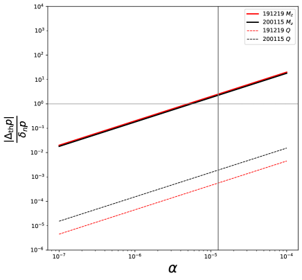
Figure 1: The ratios of the theoretical bias to the statistical error increases with the coupling constant $\alpha$. Colors represent different BH-NS binaries. The solid lines and the dashed lines represent $\frac{|\Delta_{\rm th}\ln M_{z}|}{\delta_{n}\ln M_{z}}$ and $\frac{|\Delta_{\rm th}\ln Q|}{\delta_{n}\ln Q}$, respectively. The vertical line indicates the upper bound on $\alpha$ imposed by the Cassini spacecraft.

VI Conclusions and Discussions

We have obtained the self-consistent gravitational waveforms in an expanding Universe in the Brans-Dicke theory. There are three GW polarizations, i.e., the plus polarization $h_{+}$, the cross polarization $h_{\times}$, and the breathing polarization $h_{b}$. The waveforms of these three polarizations can be applied to high redshift GW sources. In the GR limit ($\bar{\omega}\to\infty$) or when the redshift of GW source is negligible ($z\ll 1$), the waveforms converge to the previously known results.

We have considered the modifications during wave generation and propagation. Previous researches on standard sirens in modified gravity theories have adopted inconsistent waveforms which has ignored the modifications from wave generation; but the waveforms that focus on the wave generation effects, such as the post-Newtonian waveforms, apply only to the local wave zone and cannot be used directly to study GW sources with non-negligible redshifts. Compared with GR, in wave generation, there are extra breathing polarization as well as phase and amplitude corrections to the tensor polarizations; in wave propagation, the electromagnetic luminosity distance $D_{L}$ is replaced by the gravitational distance $D_{G}$ and the scalar distance $D_{S}$. The expression of $D_{G}$ has been derived before, e.g., Dalang et al. (2020), while $D_{S}$ is a new result. Inconsistent waveforms can bias the source parameters measured by the GW detectors. The main contribution to parametric estimation biases is from the phase correction of the frequency domain waveforms originating from scalar dipole radiation. This shows that the expanding of Universe will not suppress the modification of the waveforms due to the scalar dipole radiation. We found that, when the coupling constant $\alpha$ approached the Cassini upper bound, in the detection of BH-NS binaries (GW191219 and GW200115) by the Einstein Telescope, the inconsistent waveforms would bias the measurement of redshifted chirp mass significantly but had negligible impact on the measurement of the distance.

The solution to the geometric optics equations, Eq. (58), is a general result which can be applied to the GWs emitted by any isolated sources, such as a binary with a precessing orbital plane Calderón Bustillo et al. (2017), an extreme mass ratio inspiral system Yunes et al. (2012), a triple system Zhao et al. (2019), etc. The method using local wave zone to match wave generation and wave propagation can also be used in other theories, such as massive Brans-Dicke theory Liu et al. (2020), reduced Horndeski theory Dalang et al. (2021), Chern-Simons theory Yagi et al. (2012); *PhysRevD.93.029902, etc. It is interesting to consider using this match procedure to combine the parametrized post-Einsteinian (ppE) framework Tahura and Yagi (2018); *PhysRevD.101.109902 with the generalized GW propagation (gGP) framework Nishizawa (2018); *PhysRevD.97.104038; *PhysRevD.99.104038. The ppE framework mainly focuses on wave generation in modified gravity theories while the gGP framework deals with the wave propagation.

In addition to the modification of GW waveforms, modified gravity can influence the cosmological background evolution Belgacem et al. (2019b); D’Agostino and Nunes (2019). It is necessary to include all these effects to study standard sirens in the Brans-Dicke theory. We leave this for future work.