Rate-Optimal Contextual Online Matching Bandit

Abstract

Two-sided online matching platforms have been employed in various markets. However, agents’ preferences in the present market are usually implicit and unknown, and thus must be learned from data. With the growing availability of side information involved in the decision process, modern online matching methodology demands the capability to track dynamic preferences for agents based on the contextual information. This motivates us to consider a novel Contextual Online Matching Bandit prOblem (COMBO), which allows dynamic preferences in matching decisions. Existing works focus on multi-armed bandit with static preference, but this is insufficient: the two-sided preference changes as long as one-side’s contextual information updates, resulting in non-static matching. In this paper, we propose a Centralized Contextual - Explore Then Commit (CC-ETC) algorithm to adapt to the COMBO. CC-ETC solves online matching with dynamic preferences. In theory, we show that CC-ETC achieves a sublinear regret upper bound $\mathcal{O}(\log(T))$ and is a rate-optimal algorithm by proving a matching lower bound. In the experiments, we demonstrate that CC-ETC is robust to variant preference schemes, dimensions of contexts, reward noise levels, and context variation levels.

Keywords: Contextual bandits, Online decision making, Reinforcement learning, Regret analysis, Two-sided market

1 Introduction

Two-sided online matching platforms have been employed in various marketplaces such as ride-sharing, housing, job seeking, and dating markets (Gale and Shapley, 1962; Roth, 1984; Gusfield and Irving, 1989; Kamecke, 1992; Knuth, 1997; Abdulkadiroğlu and Sönmez, 1999; Roth, 2008; Mine et al., 2013; Almalis et al., 2014; Zap et al., 2018; Lokhandwala and Cai, 2018; Shi et al., 2022). In modern matching platforms, preferences are often implicit and unknown to the center platform and to market’s participants (agents) themselves, which implies that agents are uncertain about their preferences relative to the other side’s agents in the matching process. The underlying difficulty of the matching process is due to the limited resources in these markets. Consequently, agents need to compete with each other to match their own best resources. The ultimate goal is to design an optimal policy to maximize long-term interests.

We use the job seeking as our running example. The recruitment agencies want to send out interviews to the best job applicants on their preference list during hiring seasons. However, their preferences over job applicants are unknown/unclear in real scenarios. In order to hire the best candidate, a recruitment agency must estimate their preference list over job applicants correctly. Meanwhile, job applicants have the flexibility to choose the most acceptable job offer they have received based on their preferences. When the preference is static, this two-sided matching problem with one side unknown preference has been addressed by Liu et al. (2020) through the statistical decision method (bandit) (Lattimore and Szepesvári, 2020). However, it remains an open question how to address the case when contextual information of job applicants is available and how does it affect the matching result over time.

The matching platform aims to provide the most suitable job applicant to companies over time to maximize the matching utility. However, since companies are usually unable to estimate their true preferences over constantly changing job applicants. Thus, dynamic matching becomes difficult. This multi-agent competing matching problem differs from the standard i.i.d assumption in supervised learning tasks where all agents can get i.i.d job applicants’ profiles. This process is hampered by the bandit feedback (Lattimore and Szepesvári, 2020). That is, the company only receives feedback (the satisfactory level) from the matched job applicant, but does not observe (counterfactual) feedback for alternate job applicants. Meanwhile, the matched job applicant depends on all previous matching results, which means the current step’s feedback will also affect the next step’s action.

With the growing availability of side information involved in the decision process (Li et al., 2010; Abbasi-Yadkori et al., 2011; Wang et al., 2021), two-sided matching markets can utilize contextual information such as personal profiles and user preferences to make personalized decisions. The integration of contextual information will contribute to a dynamic shift in agents’ preferences from one side of the market to the other side. Consequently, varying contextual information will result in a dynamic preference in online matching. For example, job applicants regularly update their skills, experiences, and wage expectations. In this scenario, companies will shift their preferences over job applicants since job applicants’ skills change (Guo et al., 2016). Therefore, it is crucial to study how to efficiently use such varying contextual information to improve the matching result in the two-sided matching problem.

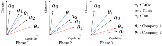
Figure 1: Arm $a_{1}$’s profile changes with an angular velocity, which results in different optimal matching results. Phase 1’s optimal matching: (company 1, Luke), (company 2, Yuna), Phase 2’s optimal matching: (company 1, Yuna), (company 1, Luke), and Phase 3’s optimal matching: (company 1, Yuna), (company 2, Luke).

In Figure 1, we present an example to illustrate the dynamic preference in the contextual online matching market. In this example, there are two companies (company 1, company 2) and three job applicants (Luke, Yuna, Ian). Job applicants’ profiles are represented in two dimensions, capability level (x-axis) and character level (y-axis). Company 1 and Company 2’s true parameters are represented by $\{{\bm{\mathbf{{\theta}}}}_{1},{\bm{\mathbf{{\theta}}}}_{2}\}\in\mathbb{R}^{2}$, where entries in ${\bm{\mathbf{{\theta}}}}_{1},{\bm{\mathbf{{\theta}}}}_{2}$ indicate the preference magnitude of the capability and character for job applicants from company 1 and company 2, respectively. All job applicants share the same preference, i.e., they all prefer company 1 to company 2. Luke’s profile is being constantly updated from Phase 1 to Phase 3, and other applicants’ profiles are fixed. Suppose the preference from the company to the job applicant is determined by the inner product $\langle{\bm{\mathbf{{\theta}}}}_{i},x_{a}\rangle$, where $x_{a}$ is the job applicant $a$’s profile, $a\in\{\text{Luke},\text{Yuna},\text{Ian}\}$. The larger the inner product is, the more preferable the job applicant is. We find that as Luke’s profile updates, the optimal matching is changing as well. This is the main challenge in the contextual online matching market. Detailed analysis of different matching scenarios is available in Section 5.2.

The major goal of this paper is to address the question of online matching problem with dynamic preferences. In previous literature, Liu et al. (2020) assumed that preferences from agents to arms are static. However, this setting could not handle the dynamic preferences scenario caused by the change of arms’ contexts; Jagadeesan et al. (2021) considered the matching with utility (money) transfer between arms and agents in the ride-sharing platform. This is not directly applicable in the hiring market since there is no utility transfer between agents and arms. They maximize the total utility from the viewpoint of the platform rather than agents. We aim to provide judicious policy for agents in this online matching market with dynamic preferences.

1.1 Major Contributions

The contributions of our proposal can be categorized into two parts. The methodological contribution is the formulation of the Contextual Online Matching Bandit prOblem (COMBO) and the introduction of an efficient Centralized Contextual - Explore Then Commit (CC-ETC) algorithm. The theoretical contribution is to provide the regret upper bound of CC-ETC, and a matching instance-dependent regret lower bound to demonstrate that CC-ETC is a rate-optimal algorithm.

Methodology. We provide a novel formulation of the COMBO with the dynamic preference in the two-sided matching market in Section 2.1. Such a formulation effectively captures the dynamic preference from agents to arms due to the arms’ varying contexts.

The CC-ETC algorithm (Algorithm 1) in Section 3 is a novel centralized multi-agent contextual competing decision-making algorithm that resolves COMBO. Our algorithm incorporates the dynamic contextual information into the deferred-acceptance algorithm (Gale and Shapley, 1962) while using the bandit framework, to solve the COMBO. We extend the single-agent ETC algorithm (Lattimore and Szepesvári, 2020) to the multi-agent ETC in COMBO over the centralized platform. We find that with sufficient exploration of arms’ contextual information, the penalized least square estimator with $l_{2}$ penalization can recover the true parameter of agents and discover the optimal matching with high probability. Our algorithm is robust to different preferences from arms to agents. It shows consistent performance in the versatile matching environment, for example, when the optimal stable matching changes rapidly over time. In Section 6, we study the performance of CC-ETC with five different scenarios. These five scenarios demonstrate that CC-ETC is robust to different changes in contexts’ schemes, various preference schemes, different contextual dimensions, and different sizes of arms and agents.

Theory. Our main result establishes that CC-ETC achieves a rate-optimal expected cumulative regret that scales logarithmically with the horizon length $T$. Due to the shifting contextual information of arms, agents to arms’ preferences are constantly shifting. These shifting preferences make our proof much more challenging than that in Liu et al. (2020), where the latter only considers fixed agents to arm’s preferences over time. Specifically, we utilize new non-asymptotic concentration results for the online ridge regression techniques (Li et al., 2021) to quantify the invalid ranking probability in the exploitation stage. This invalid ranking result is the key for deriving logarithmic regret upper bound of CC-ETC.

Importantly, we also derive a matching instance-dependent regret lower bound to demonstrate that CC-ETC is rate-optimal. Specifically, we first construct a problem instance of two-agent and three-arm in COMBO to analyze the instantaneous regret. We then categorize the regret occurring cases to decompose the instantaneous regret as a function of correcting ranking probability. Then, we use a sharp Gaussian lower tail to analyze the probability of the correcting ranking. Combining all these results, we show that the matching algorithm for COMBO will at least have a logarithmic regret. To the best of our knowledge, our algorithm obtains the first individual regret bound in the centralized contextual online matching scenario, and achieves an optimal regret bound $\Omega(\log(T))$.

1.2 Related Literature

This section discusses four lines of related literature.

Matching in Two-Sided Markets. We first discuss the matching in discrete and continuous two-sided markets when the preference from both sides are known to the platform. Gale and Shapley (1962) studied the two-sided matching markets as a pioneer and proposed the deferred-acceptance algorithm (also known as the GS algorithm), which achieved the stable matching. This algorithm (Roth, 2008) has been widely used to match hospitals with residents (Roth, 1986) and students with public schools (Atila et al., 2005; Abdulkadiroğlu et al., 2005) in New York City and Boston. They focused on discrete two-sided matching models without money transfer. Kojima et al. (2018); Nguyen and Vohra (2019); Aziz et al. (2021) focused on the two-sided market with side constraint, e.g., different races should have the same admitting proportions in the college admission. However, these results assume that the preference from both sides are known to the platform, which is fundamentally different from our setting, where agents on the one side of the market’s preferences are unknown and need to be learned through historical interactions.

Bandit and Reinforcement Learning Approaches. Bandit algorithms (Lattimore and Szepesvári, 2020) and reinforcement learning (Sutton and Barto, 2018) are modern strategies to solve sequential decision making problems. They have received attentions in statistics community for business and scientific applications including dynamic pricing (Wang et al., 2020; Chen et al., 2021), online decision making (Shi et al., 2022; Chen et al., 2021), dynamic treatment regimes (Luckett et al., 2019; Qi et al., 2020), and online causal effect in two-sided market (Shi et al., 2022). The two-sided competing matching problem can be transformed into a sequential decision-making problem (Das and Kamenica, 2005; Liu et al., 2020; Sarkar, 2021). To tackle the two-sided matching problem in the bandit framework, researchers transform the matching objects into bandit notation and assume that one side of market participants can be represented as agents (preferences are unknown) and the other side participants of the market can be viewed as arms (preferences are known), and transform this problem into a multi-agent bandit competing problem. Liu et al. (2020) considered that an agent could only match with one arm at one time, such as in the dating market, where Sarkar (2021) considered the case that an agent could match with multiple arms, such as in the lending market. However, these works do not consider the arms’ contextual information and hence are not capable of tackling our dynamic matching problem.

Centralized Two-sided Matching Market. In practice, there usually exists a centralized platform helping agents to match with each other, which exhibits the same setting as our COMBO. Liu et al. (2020) is one of the first work which considers the case that agents need to learn their preferences through bandit techniques in the centralized platform. Jagadeesan et al. (2021) considers that both sides’ preferences are represented by utility functions over contexts and allow money transfer. They optimize the total utility in the viewpoint of the platform, which is different from ours. We focus on minimizing the individual agent’s regret and considering the case where there is no money transfer among agents. For example, monetary transfer is prohibited in the job application market. In a similar setting, Cen and Shah (2021) considers the case when both users and providers do not know their true preferences a priori and incorporate costs and money transfers among agents to faithfully model the competition among agents and discuss the fairness in the matching. Min et al. (2022) considers the uncertain utility of matching two agents in the episodic reinforcement learning setting. Li et al. (2023) studied the two-sided matching market with complementary preference with quota constraints. However, none of the current work considers the case when preference is allowed to change due to dynamic contextual information.

Decentralized Two-sided Matching Market. The last related line of work considers decentralized platform when there is no central clearinghouse. Agents in the decentralized two-sided matching problem (Sankararaman et al., 2020; Vial et al., 2021; Liu et al., 2021; Dai and Jordan, 2021a, b) are allowed to collaborate. This is useful in applications like games. Because of this, methods and analysis tools are fundamentally different from those in the centralized problem. These decentralized works can not be directly applied to COMBO since COMBO uses a centralized platform.

The organization of this paper is as follows. In Section 2, we formulate the contextual online matching problem in two-sided markets and provide the CC-ETC algorithm in Section 3. The theoretical regret upper bound of CC-ETC is provided in Section 4. In Section 5, we present an example with two agents and three arms in the two-sided market and provide an instance-dependent lower bound to demonstrate that our algorithm is rate-optimal. In addition, we design experiments to demonstrate the empirical effectiveness and robustness of our proposed method in Section 6.

We denote $[N]=[1,2,...,N]$ where $N$ is a positive integer. Define the capital $X\in\mathbb{R}^{d}$ be the $d$-dimensional random vector. Let $\textbf{0}_{d}=\{0,0,...,0\}^{\sf T}\in\mathbb{R}^{d}$ represent a $d$-dimensional zero vector. The bold ${\bm{\mathbf{{X}}}}\in\mathbb{R}^{d\times d}$ represents a real valued matrix. Let ${\bm{\mathbf{{I}}}}_{d}=\text{diag}(1,1,...,1)\in\mathbb{R}^{d\times d}$ represent a $d\times d$ diagonal identity matrix. We denote $T$ as the time horizon.

2 Problem

This section formulates the contextual online matching problem and discusses its challenges caused by the dynamic contexts.

2.1 Problem Formulation

We now describe the problem formulation for the Contextual Online Matching Bandit prOblem (COMBO). The matching of job applicants and hiring companies will be our running example throughout the paper. We first introduce notations and six necessary elements in COMBO.

(I) Environment. There are $N$ companies (agents) denoted by $\mathcal{N}=\{p_{1},p_{2},...,p_{N}\}$ and $K$ job applicants (arms) denoted by $\mathcal{K}=\{a_{1},a_{2},...a_{K}\}$ in the centralized platform. We assume the number of companies $N$ is smaller than the number of job applicants $K$.

(II) Preference. We next present the preferences of both sides. There are two kinds of preference: arms to agents’ preferences, agents to arms’ preferences.

Arms to agents’ fixed and known preference $\pi:\mathcal{K}\mapsto\mathcal{N}$. We assume there exist true fixed preferences from job applicants to companies, and these preferences are available for the centralized platform. For example, job applicants are usually required to submit their preferences for different companies on the platform. We denote $\pi_{j,i}$ as the rank order for company $p_{i}\in\mathcal{N}$ from the viewpoint of the job applicant $a_{j}$, and assume there is no tie of ranks. Suppose the centralized platform knows the fixed preferences from job applicants to companies, represented as ${\bm{\mathbf{{\pi}}}}_{j}=\{\pi_{j,1},...,\pi_{j,N}\},\forall a_{j}\in\mathcal{K}$. In other words, ${\bm{\mathbf{{\pi}}}}_{j}$ is a permutation of $[N]$. And $\pi_{j,i}<\pi_{j,i^{\prime}}$ implies job applicant $a_{j}$ prefers the company $p_{i}$ over the company $p_{i^{\prime}}$. As a shorthand, the notation $p_{i}<_{j}p_{i^{\prime}}$ means that the job applicant $a_{j}$ prefers the company $p_{i}$ over the company $p_{i^{\prime}}$. When the arm $a_{j}$ is clear from context, we simply write $p_{i}<p_{i^{\prime}}$. This known arm-to-agent preference is a mild and common assumption in current matching literature (Liu et al., 2020, 2021; Li et al., 2023).

Agents to arms’ dynamic and unknown preference $r(t):\mathcal{N}\mapsto\mathcal{K},\forall t\in[T]$. Preferences from companies to arms are dynamic over time and are unknown to the platform and agents. The platform’s goal is to learn companies’ dynamic preferences over job applicants. We denote $r_{i,j}(t)$ as the rank order for the job applicant $a_{j}$ from the viewpoint of the company $p_{i}$ at time $t$ and we also assume there is no tie of ranks. We use ${\bm{\mathbf{{r}}}}_{i}(t)=\{r_{i,1}(t),...,r_{i,K}(t)\}$ to represent the preference from the company $p_{i}\in\mathcal{N}$ to all job applicants at time $t$. In other words, ${\bm{\mathbf{{r}}}}_{i}(t)$ is a permutation of $[K]$. We denote $r_{i,j}(t)<r_{i,j^{\prime}}(t)$ as the company $p_{i}$ prefers the job applicant $a_{j}$ over the job applicant $a_{j^{\prime}}$ at time $t$. Similarly, $a_{j}<_{i}^{t}a_{j^{\prime}}$ means that the company $p_{i}$ prefers the job applicant $a_{j}$ over the job applicant $a_{j^{\prime}}$ at time $t$.

(III) Stable Matching and Optimal Matching. Before defining regret, we introduce several key concepts in the matching field. First, a stable matching (Gale and Shapley, 1962) of agents and arms is one where no pair of agent and arm would prefer to be matched with each other over their respective matches. Given full preferences’ information from both sides of the market, arm $a_{j}$ is called a valid match of agent $p_{i}$ if there exist a stable matching according to those rankings such that $a_{i}$ and $p_{j}$ are matched. Given these definitions, we can now introduce an optimal matching in COMBO. Arm $a_{j}$ is an optimal matching of agent $p_{i}$ if it is the most preferred valid match. Given full complete information of preferences, the Gale-Shapley (GS) algorithm is known to produce a stable matching. Details of the GS algorithm can be checked in Appendix A2. The matching result by the GS algorithm is always optimal for each member of the proposing side. We use $\overline{m}_{i}(t)$ to represent the agent-optimal matching object for agent $p_{i}$ at time $t$. We denote $\overline{{\bm{\mathbf{{m}}}}}(t)=\{\overline{m}_{1}(t),....,\overline{m}_{N}(t)\}$ as the agent-optimal matching function from $\mathcal{N}$ to $\mathcal{K}$ at time $t$, which is determined by both sides’ true preferences at time $t$.

(IV) Matching Policy ${\bm{\mathbf{{m}}}}(t)$. At each time step $t$, for the company $p_{i}$, platform assigns a job applicant $m_{i}(t)$ as the recommended job applicant, where $m_{(\cdot)}(t)\overset{\Delta}{=}{\bm{\mathbf{{m}}}}(t)$ is an injective function from the set of companies $\mathcal{N}$ to the set of job applicants $\mathcal{K}$ at time $t$. $m_{(\cdot)}(t)$, the recommended job applicants’ assignment functions for each agent, are not only determined by the proposal from the agent $p_{i}$, but also by the competing status with other companies and job applicants’ preferences. Besides, a centralized platform, e.g., LinkedIn, exists in this competing environment to coordinate this matching process.

(V) Matching Score $y$. At time $t$, if the company (agent) $p_{i}$ is matched with a job applicant (arm) $a_{j}$, the company $p_{i}$ obtains a noisy matching score $y_{i,j}(t)$, which measures the satisfaction of the matching. Each job applicant’s profile (contextual information) ${\bm{\mathbf{{x}}}}_{j}(t)\in\mathbb{R}^{d}$ at each time step $t$ is available to the platform, which includes demographic, geographic, or platform usage information. Given the contextual information ${\bm{\mathbf{{x}}}}_{j}(t)$ from the matched job applicant $a_{j}$, we assume that the noisy matching score $y_{i,j}(t)$ follows the stochastic linear bandit (Lattimore and Szepesvári, 2020) model,

$$y_{i,j}(t)=\mu_{i,j}(t)+\epsilon_{i,j}(t),$$ (1)

where we define $\mu_{i,j}(t)={\bm{\mathbf{{\theta}}}}_{i,*}^{\sf T}{\bm{\mathbf{{x}}}}_{j}(t)$ as the mean matching score at time $t$ if the company $p_{i}$ is matched with the job applicant $a_{j},\forall i\in[N],j\in[K],t\in[T]$. ${\bm{\mathbf{{\theta}}}}_{i,*}\in\mathbb{R}^{d}$ is the true parameter for company $p_{i}$ that summarizes the relation between the context ${\bm{\mathbf{{x}}}}_{j}(t)$ and the noisy matching score $y_{i,j}(t)$. True parameter’s coordinate expresses its preference magnitude over contexts. For example, coordinate ${\bm{\mathbf{{\theta}}}}_{i,*}^{(1)}\in\mathbb{R}$ represents the capability preference level, and coordinate ${\bm{\mathbf{{\theta}}}}_{i,*}^{(2)}\in\mathbb{R}$ represents the character preference level, as it shown in Figure 1. The noise $\epsilon_{i,j}(t)$’s are drawn independently from a $\sigma$-subgaussian distribution for $t\in[T],i\in[N],j\in[K]$. That is, for every $\alpha\in\mathbb{R}$, it is satisfied that $\mathbb{E}[\exp(\alpha\epsilon_{i,j}(t))]\leq\exp(\alpha^{2}\sigma^{2}/2)$. One goal of the centralized platform is to learn each company’s preference magnitude (true parameter) to improve its recommendation performance over time.

(VI) Regret. Based on model (1), at time $t$, when company $p_{i}$ is matched with the assigned job applicant $m_{i}(t)$, a noisy matching score $y_{i}(t)\overset{\Delta}{=}y_{i,m_{i}(t)}(t)$ is observed. The mean reward $\mu_{i,m_{i}(t)}(t)$ represents the noiseless feedback (such as the satisfaction level) of company $p_{i}$ with respect to its assigned matching job applicant $m_{i}(t)$. Thus the cumulative agent-optimal (company-optimal) stable regret for the agent $p_{i}$ is defined as

$$R_{i}(T):=\sum_{t=1}^{T}\mu_{i,\overline{m}_{i}(t)}(t)-\sum_{t=1}^{T}\mu_{i,m_{i}(t)}(t).$$ (2)

This agent-optimal regret represents the difference between the capability of a policy ${\bm{\mathbf{{m}}}}_{i}\overset{\Delta}{=}\{m_{i}(1),m_{i}(2),...,m_{i}(T)\}$ in hindsight and the optimal stable matching oracle policy $\overline{m}_{i}$. Our goal is to design an algorithm for agents to minimize the cumulative agent-optimal regret over the time horizon $T$.

2.2 Challenges and Resolutions

The challenges of this contextual online matching bandit problem arise from changing contexts, resulting in dynamic unknown preferences. In order to precisely evaluate dynamic preferences, we need to learn them from historical data, which is affected by the designed policy. A good algorithm should balance the trade-off between minimizing cumulative agent-optimal stable regret and achieve the true stable matching as many as possible.

2.2.1 Challenge 1: Preference estimation given shifting job applicants’ profiles

Learning companies’ preferences given shifting job applicants’ profiles is challenging since there are massive numbers of possible matchings between companies and job applicants. Recovering preference signals from noisy matching scores requires modeling the relationship between companies and job applicants. We resolve this challenge by considering the linear relationship between the matching score and job applicants’ profiles. The main statistical task is to estimate the underlying preference parameters by conducting matching experiments. Such an estimate is indispensable for inferring a true preference scheme and informing future matching decisions.

2.2.2 Challenge 2: Balance exploration and exploitation

The platform needs to balance the exploration (collecting enough job applicants’ profiles and companies’ matching information) to estimate companies’ true preference parameters and the exploitation (providing the optimal matching for companies) at each matching time point. Compared to the single-agent bandit problem, the multi-agent competing matching problem is more challenging since the platform needs to handle the multi-agent exploration and exploitation trade-off. We resolve this challenge by using the Explore-Then-Commit strategy (Lattimore and Szepesvári, 2020) to balance the exploration-exploitation trade-off and the incapable exploration for some specific matching patterns. The main technical challenge is identifying the optimal length of the exploration stage for these companies.

2.2.3 Challenge 3: Rate-optimality of ETC strategy in COMBO

The third challenge is to show that the proposed ETC strategy is rate-optimal. Such rate optimality is more challenging than that in the static preference setting. In the static setting, the preference scheme is time-invariant, and the companies’ preference scheme is independent of job applicants’ profiles. The technical challenge of proving such rate optimality is resolved by developing a probability upper bound for the valid ranking and a probability lower bound for the correct ranking, where definitions of the valid ranking and the correct ranking can be found in Section A4.2 and Section A6, separately. The valid ranking result is the key to deriving logarithmic matching regret upper bound; the correct ranking result is the key to building the logarithmic lower bound for the matching algorithms to solve COMBO.

3 Algorithm

In this section, we propose the CC-ETC algorithm to learn all agents’ true parameters ${\bm{\mathbf{{\theta}}}}_{i,*},\forall i\in[N]$ and to maximize the agent-optimal expected payoff. The CC-ETC algorithm is composed of two parts, the exploration stage, and the exploitation stage. The benefit of using the ETC algorithm is that it can explore enough matching patterns by design to avoid the incapable exploration of specific matching patterns. In the exploration stage, the centralized platform assigns job applicants to companies cyclically, ensuring that each company can receive all job applicants’ time-varying profiles. When the exploration stage ends, we estimate agents’ true parameters, which will be used to estimate companies’ dynamic preferences over job applicants. Then companies will be matched with these recommended job applicants via the GS Algorithm. Finally, the detailed CC-ETC algorithm is summarized in Algorithm 1.

1 Input: Time horizon $T$; exploration loop $h$; ridge parameters $\lambda_{i},\forall i\in[N]$; preference ${\bm{\mathbf{{\pi}}}}_{j},\forall j\in[K]$.

2 Explore: Get all companies’ estimated true parameters: $(\widehat{{\bm{\mathbf{{\theta}}}}}_{1}(\overline{h}),...,\widehat{{\bm{\mathbf{{\theta}}}}}_{N}(\overline{h}))$ = Exploration($\mathcal{N}$, $\mathcal{K}$, ${\bm{\mathbf{{\pi}}}}_{j\in[K]}$, $\lambda_{i\in[N]}$, $h$) from Algorithm 2.

3 Exploit: Get the matching result: Exploitation(T, $\mathcal{N},\mathcal{K}$, ${\bm{\mathbf{{\pi}}}}_{j\in[K]}$, $\widehat{{\bm{\mathbf{{\theta}}}}}_{i\in[N]}(\overline{h})$) from Algorithm 3.

Algorithm 1 CC-ETC

We first review the GS matching algorithm (Gale and Shapley, 1962) which can achieve the stable matching result when both sides’ true preferences are known to the platform. The detail of the GS Algorithm 4 under the job application scenario is in Appendix A2.

3.1 Exploration Stage

We first denote the exploration length as $\bar{h}=h\binom{K}{N}$, where $h$ is the exploration loops. The determination of the exploration loops is provided in Eq. (7). In each matching loop, there is a total of $\binom{K}{N}$ rounds to force each company to match with all job applicants. For example, when $t\leq\bar{h}$, company $p_{i}$ matches with the platform assigned job applicant $m_{i}(t)=a_{j}$ and then receives the noisy reward $y_{i,m_{i}(t)}(t)$.

At the end of $t=\overline{h}$, we calculate the estimated preference parameter $\widehat{{\bm{\mathbf{{\theta}}}}}_{i}(t)$ of company $p_{i}$ through the collection of profiles and noisy matching scores up to time $\overline{h}$. Let ${\bm{\mathbf{{X}}}}_{i}(t)=[{\bm{\mathbf{{x}}}}_{i}(1),{\bm{\mathbf{{x}}}}_{i}(2),...,{\bm{\mathbf{{x}}}}_{i}(t)]^{{}^{\sf T}}\in\mathbb{R}^{t\times d}$ denotes the company $p_{i}$’s collection of matched job applicants’ profiles up to time $t$, where ${\bm{\mathbf{{x}}}}_{i}(t)$ represents the matched job applicant’s profile at time $t$. We also define ${\bm{\mathbf{{y}}}}_{i}(t)=[y_{i}(1),y_{i}(2),...,y_{i}(t)]^{\sf T}\in\mathbb{R}^{t}$ as the company $p_{i}$’s collection of noisy matching scores vector up to time $t$, where $y_{i}(t)$ represents the collected noisy matching score after matched with the corresponding job applicant for company $p_{i}$ at time $t$. We define the filtration $\mathcal{F}_{i}(t)$ that is generated by random variables $\{X_{i}(1),...,X_{i}(t),Y_{i}(1),...,Y_{i}(t)\}$. With these collected information $\mathcal{F}_{i}(\overline{h})$, the true preference parameter ${\bm{\mathbf{{\theta}}}}_{i,*}$ for company $p_{i}$ will be estimated by minimizing the mean square error with an $l_{2}$ loss on the true parameter. Specifically, the penalized optimization problem is

$$\underset{{\bm{\mathbf{{\theta}}}}_{i}\in\mathbb{R}^{d}}{\min}\left\lVert{\bm{\mathbf{{y}}}}_{i}(\overline{h})-{\bm{\mathbf{{X}}}}_{i}(\overline{h}){\bm{\mathbf{{\theta}}}}_{i}\right\rVert_{2}^{2}+\lambda_{i}\left\lVert{\bm{\mathbf{{\theta}}}}_{i}\right\rVert_{2}^{2},\quad\forall i\in[N],$$ (3)

where the ridge parameter $\lambda_{i}$ is used to ensure the loss function in (3) has a unique minimizer even when previous matched job applicants’ profiles for company $p_{i}$ does not span $\mathbb{R}^{d}$. The corresponding ridge estimator for company $p_{i}$ is

$$\widehat{{\bm{\mathbf{{\theta}}}}}_{i}(\overline{h})=\big{(}{\bm{\mathbf{{X}}}}_{i}(\overline{h})^{\sf T}{\bm{\mathbf{{X}}}}_{i}(\overline{h})+\lambda_{i}{\bm{\mathbf{{I}}}}\big{)}^{-1}{\bm{\mathbf{{X}}}}_{i}(\overline{h})^{\sf T}{\bm{\mathbf{{y}}}}_{i}(\overline{h}),\quad\forall i\in[N],$$ (4)

where the choice of the optimized $\overline{h}$ will be provided and illustrated in Section 4. The exploration algorithm is available in Algorithm 2. From lines 5-10, the platform sequentially updates the collected contextual information ${\bm{\mathbf{{\Sigma}}}}_{i}(t)$ and scores’ information ${\bm{\mathbf{{S}}}}_{i}(t)$ for each company. In the end, CC-ETC obtains the estimated parameter $\widehat{{\bm{\mathbf{{\theta}}}}}_{i}(t)$ for all agents.

1 Input: Number of companies $N$; number of job applicants $K$; preference ${\bm{\mathbf{{\pi}}}}_{j},\forall j\in[K]$; ridge parameters $\lambda_{i},\forall j\in[N]$; exploration loop $h$.

2 Initialize: ${\bm{\mathbf{{\Sigma}}}}_{i}(0)=\lambda_{i}{\bm{\mathbf{{I}}}}_{d}$, ${\bm{\mathbf{{S}}}}_{i}(0)=\textbf{0}_{d}$, $\widehat{{\bm{\mathbf{{\theta}}}}}_{i}(0)=\textbf{0}_{d}$, for $\forall i\in[N]$.

3 Exploration Stage

4 for $z\in\{1,...,h\}$ do

5       for $t\in\{(z-1)\binom{K}{N}+1,(z-1)\binom{K}{N}+2,...,z\binom{K}{N}\}$ do

6             for $i\in\{1,...,N\}$ do

7                   Matching: Assign the job applicant $m_{i}(t)$ for company $p_{i}$.

8                   Collecting: Receive matching score $y_{i}(t)$ for company $p_{i}$.

9                   Updating: Online update the collected information for company $p_{i}$. ${\bm{\mathbf{{\Sigma}}}}_{i}(t)={\bm{\mathbf{{\Sigma}}}}_{i}(t-1)+{\bm{\mathbf{{x}}}}_{m_{i}(t)}(t){\bm{\mathbf{{x}}}}_{m_{i}(t)}(t)^{\sf T},{\bm{\mathbf{{S}}}}_{i}(t)={\bm{\mathbf{{S}}}}_{i}(t-1)+{\bm{\mathbf{{x}}}}_{m_{i}(t)}(t)y_{i}(t).$

10for $i\in\{1,...,N\}$ do

11       Estimating: Output the estimated parameter $\widehat{{\bm{\mathbf{{\theta}}}}}_{i}(\overline{h})={\bm{\mathbf{{\Sigma}}}}_{i}^{-1}(t){\bm{\mathbf{{S}}}}_{i}(t)$.

Algorithm 2 Exploration

3.2 Exploitation Stage

In the exploitation stage (Algorithm 3), with the estimated preference parameter $\widehat{{\bm{\mathbf{{\theta}}}}}_{i}(\overline{h})$, company $p_{i}$ can estimate its rankings for all arms at time $t(\geq\overline{h}+1)$. For example, at time step $t=\overline{h}+1$, company $p_{i}$ can first estimate all job applicants’ mean score

$$\hat{\mu}_{i,j}(t)=\langle\widehat{{\bm{\mathbf{{\theta}}}}}_{i}(\overline{h}),{\bm{\mathbf{{x}}}}_{j}(t)\rangle,\quad\forall i\in[N],j\in[K].$$ (5)

Then company $p_{i}$ ranks all job applicants according to its estimated mean reward $\hat{\mu}_{i,j}(t)$ in descending order. Finally, all rankings estimated by companies will be submitted to the centralized platform. See line 4 to line 5 in Algorithm 3. Here we denote the estimated rankings of all job applicants for the company $p_{i}$ as $\hat{{\bm{\mathbf{{r}}}}}_{i,[K]}(t)=\{\hat{r}_{i,1}(t),...,\hat{r}_{i,K}(t)\}$, which depends on the estimated mean reward $\hat{{\bm{\mathbf{{\mu}}}}}_{i,[K]}(t)=\{\hat{\mu}_{i,1}(t),...,\hat{\mu}_{i,K}(t)\}$. Here the estimated ranking $\hat{{\bm{\mathbf{{r}}}}}_{i,[K]}(t)$ is a permutation of $[K]$ and $\hat{\mu}_{i,j}(t)>\hat{\mu}_{i,j^{\prime}}(t)$ is equivalent to $\hat{r}_{i,j}(t)<\hat{r}_{i,j^{\prime}}(t)$. After the platform collects all rankings from companies, the platform will match companies and job applicants by the GS Algorithm. Then all companies will receive their corresponding matched job applicants and noisy matching scores at time $t$.

1 Input: Time horizon $T$; number of companies $N$; number of job applicants $K$; estimated true parameters $\widehat{{\bm{\mathbf{{\theta}}}}}_{i}(\overline{h}),\forall i\in[N]$; preference ${\bm{\mathbf{{\pi}}}}_{j},\forall j\in[K]$.

2 for $t\geq\overline{h}+1$ do

3       for $i\in\{1,...,N\}$ do

4             Ranking: Estimate the score $\hat{\mu}_{i,j}(t)=\widehat{{\bm{\mathbf{{\theta}}}}}_{i}(\overline{h})^{\sf T}{\bm{\mathbf{{x}}}}_{j}(t),\forall j\in[K]$. Rank all job applicants according to $\hat{\mu}_{i,j}(t)$ and get the ranking $\hat{{\bm{\mathbf{{r}}}}}_{i,[K]}(t)$.

5             Uploading: Company $p_{i}$ uploads the ranking $\hat{{\bm{\mathbf{{r}}}}}_{i,[K]}(t)$ to the platform.

6      Stable Matching: Platform computes stable matching ${\bm{\mathbf{{m}}}}(t)$ according to all rankings $\{\hat{{\bm{\mathbf{{r}}}}}_{1,[K]}(t),,,\hat{{\bm{\mathbf{{r}}}}}_{N,[K]}(t)\}$ and all job applicants’ preferences $\{{\bm{\mathbf{{\pi}}}}_{1},...,{\bm{\mathbf{{\pi}}}}_{K}\}$ via GS Algorithm 4.

7       for $i\in\{1,...,N\}$ do

8             Company $p_{i}$ receives the instantaneous noisy matching score $y_{i}(t)$.

Algorithm 3 Exploitation

4 Regret Upper Bound of CC-ETC

In Section 4.1, we list some useful regularity conditions. Then we establish the regret upper bound of the proposed CC-ETC in Section 4.2. In Section A4.1, we highlight the critical regret decomposition result used for the main theorem and also present the outline of the proof. In Section A4.2, we provide a key lemma to quantify the invalid ranking probability.

4.1 Regularity Conditions

For agent $p_{i}$, we use $\overline{\Delta}_{i,j}(t)=\mu_{i,\overline{m}_{i}(t)}(t)-\mu_{i,j}(t)$ to define the reward gap between the agent-optimal arm and an arbitrary arm $a_{j}$ at time $t$. Define $\mathcal{Q}_{i,\text{sub}}(t)=\{j|\overline{\Delta}_{i,j}(t)>0,j\in[K]\}$ as the set of sub-optimal arms for agent $p_{i}$ at time $t$ and $\mathcal{Q}_{i,\text{sup}}(t)=\{j|\overline{\Delta}_{i,j}(t)<0,j\in[K]\}$ as the set of super-optimal arms for agent $p_{i}$ at time $t$. Denote $\overline{\Delta}_{i,\min}(t)=\underset{j\in\mathcal{Q}_{i,\text{sub}}(t)}{\min}\overline{\Delta}_{i,j}(t)=\underset{j\in\mathcal{Q}_{i,\text{sub}}(t)}{\min}\langle{\bm{\mathbf{{\theta}}}}_{i,*},{\bm{\mathbf{{x}}}}_{\overline{m}_{i}(t)}(t)-{\bm{\mathbf{{x}}}}_{j}(t)\rangle$ as the (positive) minimum margin gap for the agent $p_{i}$ at time $t$. It is the minimum difference between an arbitrary arm $a_{j}$ from the set of sub-optimal arms and the agent-optimal stable matching arm $a_{\overline{m}_{i}(t)}$ from the viewpoint of agent $p_{i}$ at time $t$. Define $\overline{\Delta}_{i,\min}=\underset{t\in[T]}{\min}\overline{\Delta}_{i,\min}(t)$, which represents the (positive) minimum margin gap for agent $p_{i}$ over time $t\in[T]$ and is called the uniform (positive) minimum margin gap for agent $p_{i}$. Similarly, we define $\overline{\Delta}_{i,\max}(t)=\underset{j\in[K]}{\max}\overline{\Delta}_{i,j}(t)$ and $\overline{\Delta}_{i,\max}=\underset{t\in[T]}{\max}\overline{\Delta}_{i,\max}(t)$.

Assumption 1

(Uniform Minimal (Positive) Margin Condition). No arm is indifferent to the agent-optimal matching arm from the viewpoint of $p_{i}$ at each time step $t\in[T]$, that is, $\overline{\Delta}_{i,\min}>0,\forall i\in[N]$.

Our Assumption 1 generalizes the uniform minimal margin condition imposed in the static matching literature (Liu et al., 2020) to the dynamic matching COMBO. In the static matching case, the mean matching score is static. However, in our dynamic matching case, the true mean matching score $\mu_{i,j}(t)$ is shifting over time $t$, and hence we need a more tailored minimal margin condition for COMBO.

This uniform minimal margin condition represents that the uniform minimum reward gap between the arm $a_{\overline{m}_{i}(t)}$ and any other sub-optimal arms over time horizon $T$ is greater than zero. It avoids the situation that there is a tie between the agent-optimal arm and the sub-optimal arm (no ties), which includes two situations, (I) there are no two identical arms (agent-optimal and sub-optimal arm) over time $t$; (II) there is no symmetric arms at any time, which means

$$\overline{\Delta}_{i,\min}(t)>0 \Leftrightarrow\langle{\bm{\mathbf{{\theta}}}}_{i,*},\frac{{\bm{\mathbf{{x}}}}_{\overline{m}_{i}(t)}(t)-{\bm{\mathbf{{x}}}}_{j}(t)}{\left\lVert{\bm{\mathbf{{x}}}}_{\overline{m}_{i}(t)}(t)-{\bm{\mathbf{{x}}}}_{j}(t)\right\rVert_{2}}\rangle>0\Leftrightarrow\left\lVert{\bm{\mathbf{{\theta}}}}_{i,*}\right\rVert_{2}\cos({\phi_{i,j}(t)})>0,$$

where the equivalency is derived through the linear structure of matching score and the definition $\cos({\phi_{i,j}(t)})=\langle\frac{{\bm{\mathbf{{\theta}}}}_{i,*}}{\left\lVert{\bm{\mathbf{{\theta}}}}_{i,*}\right\rVert_{2}},\frac{{\bm{\mathbf{{x}}}}_{\overline{m}_{i}(t)}(t)-{\bm{\mathbf{{x}}}}_{j}(t)}{\left\lVert{\bm{\mathbf{{x}}}}_{\overline{m}_{i}(t)}(t)-{\bm{\mathbf{{x}}}}_{j}(t)\right\rVert_{2}}\rangle$. From the assumption $\overline{\Delta}_{i,\min}(t)>0$, we can imply that $\cos({\phi_{i,j}(t)})>0$. This means there is no such symmetric sub-optimal arm $a_{j}$ which is the same as the agent-optimal arm $a_{\overline{m}_{i}(t)}$ in the viewpoint of agent $p_{i}$. In the job application scenario, it means there is no such job applicant that is the same as the company-optimal job applicant evaluated by the company $p_{i}$. For example, suppose Yuna is the company-optimal applicant, and its context vector is $x_{\overline{m}_{i}(t)}=[0.2,0.8]^{\sf T}$. Luke is a sub-optimal applicant, and its context vector is $x_{j}(t)=[0.8,0.2]^{\sf T}$. If company $p_{i}$’s true parameter is ${\bm{\mathbf{{\theta}}}}_{i,*}=[1,1]^{\sf T}$, company $p_{i}$ cannot distinguish Yuna and Luke because the matching score is the same $\langle[0.2,0.8],[1,1]\rangle=\langle[0.8,0.2],[1,1]\rangle=2$. Thus, we assume there is no such symmetric case.

In the job application scenario, the interpretation of ${\bm{\mathbf{{\theta}}}}_{i,*}$ is how the company $p_{i}$ values each skill of a job applicant. Without loss of generality, we assume all elements of ${\bm{\mathbf{{\theta}}}}_{i,*}$ are non-negative. Formally, we assume the following positive weight condition:

Assumption 2

(Positive Weight Condition). We assume ${\bm{\mathbf{{\theta}}}}_{i,*}^{(r)}>0,\forall r\in[d],i\in[N]$.

4.2 Main Theorem Statement

We are now ready to provide the regret upper bound for CC-ETC.

Theorem 1

Assume Assumption 1 and Assumption 2 hold, and suppose all agents follow the CC-ETC Algorithm. Given the exploration rounds $\overline{h}=h\binom{K}{N}$ designed by CC-ETC, the agent $p_{i}$’s expected cumulative regret up to $T\geq\overline{h}$ is upper bounded by

$$R_{i}(T) \leq\underbrace{\sum_{t=1}^{\bar{h}}\overline{\Delta}_{i,m_{i}(t)}(t)}_{\text{Part I Regret}}+\underbrace{NK\Bigg{[}\sum_{t=\overline{h}+1}^{T}\overline{\Delta}_{i,\max}(t)\Bigg{]}\exp\Bigg{[}-\overline{h}\frac{\lambda_{i}^{2}\overline{\Delta}_{i,\min}^{2}}{2d^{2}{\bm{\mathbf{{x}}}}_{i,\max}^{2}\sigma^{2}}+\log(2d)\Bigg{]}}_{\text{Part II Regret}},$$ (6)

where $N$ is the number of agents, $K$ is the number of arms, $\lambda_{i}$ is the ridge hyperparameter, $\sigma$ is the reward noise level, $d$ is the context dimension, ${\bm{\mathbf{{x}}}}_{i,\max}=\left\lVert{\bm{\mathbf{{X}}}}_{i}(\overline{h})\right\rVert_{\infty}$ is the maximum absolute value of the context entry.

Proof. This detailed proof can be found in supplementary material. To derive the regret upper bound of CC-ETC algorithm in COMBO, we decompose the regret into two steps, the exploration stage, and the exploitation stage. The detailed decomposition of the regret can be found in Section A4.1. (i) In the exploration stage, the regret can be obtained as shown in Eq. (6) named “Part I Regret”; (ii) in the exploitation stage, the regret for the agent is due to the happening of “bad events”, which is quantified by the product of invalid ranking probability (the exponential term) and its corresponding instantaneous regret (the sub-optimal gap) caused by the invalid ranking from the agent. Both the invalid ranking probability and the instantaneous regret will be explained in Section A4.2.

The above theorem provides a general regret upper bound of the CC-ETC algorithm for COMBO with the given exploration rounds $\overline{h}$. Given Eq. (6), we optimize $\overline{h}$ to show CC-ETC algorithm has a logarithmic regret in the following corollary.

Corollary 1

Under assumptions of Theorem 1, if

$$\overline{h}=\max\left\{\binom{K}{N},\underset{i\in[N]}{\max}\frac{2d^{2}{\bm{\mathbf{{x}}}}_{i,\max}^{2}\sigma^{2}}{\overline{\Delta}_{i,\min}^{2}\lambda_{i}^{2}}\log\frac{TNK\lambda_{i}^{2}\overline{\Delta}_{i,\min}^{2}}{d{\bm{\mathbf{{x}}}}_{i,\max}^{2}\sigma^{2}}\right\},$$ (7)

then we have

$$R_{i}(T) \leq C_{1}(d,\sigma,\overline{\Delta}_{i,\min},\lambda_{i},{\bm{\mathbf{{x}}}}_{i,\max})\log\Bigg{[}C_{2}(N,K,d,\sigma,\overline{\Delta}_{i,\min},\lambda_{i},{\bm{\mathbf{{x}}}}_{i,\max})\times T\Bigg{]}$$ (8)

$$\quad+C_{1}(d,\sigma,\overline{\Delta}_{i,\min},\lambda_{i},{\bm{\mathbf{{x}}}}_{i,\max})+\overline{\Delta}_{i,\max}=\mathcal{O}(\log(T))$$

where the constants $C_{1},C_{2}$ are given by $C_{1}=\frac{2d^{2}{\bm{\mathbf{{x}}}}_{i,\max}^{2}\sigma^{2}\overline{\Delta}_{i,\max}}{\overline{\Delta}_{i,\min}^{2}\lambda_{i}^{2}},C_{2}=\frac{NK\lambda_{i}^{2}\overline{\Delta}_{i,\min}^{2}}{d{\bm{\mathbf{{x}}}}_{i,\max}^{2}\sigma^{2}}.$

The regret upper bound depends logarithmically on the time horizon $T$ as shown in Eq. (8). We next discuss the dependence of the upper bound on a few critical parameters. This regret upper bound depends on the context’s dimension $d$ at order $\tilde{\mathcal{O}}(d^{2})$ as shown in the definition of $C_{1}$, where $\tilde{\mathcal{O}}(\cdot)$ is up to a log-term. It also relies on the noise level $\sigma$ of the environment at order $\tilde{\mathcal{O}}(\sigma^{2})$. We find the regret upper bound depends on the uniform minimal margin condition $\overline{\Delta}_{i,\min}$ at order $\tilde{\mathcal{O}}((\overline{\Delta}_{i,\min})^{-2})$, which means that when $\overline{\Delta}_{i,\min}$ decreases, the regret will increase dramatically. From another viewpoint, if the uniform minimal margin condition becomes small, the problem becomes challenging since it is difficult for the agent to distinguish two close arms. Then the ranking provided by the agent is no longer correct. It results in the non-optimal stable matching result. Finally, when the number of agents ($N$) and arms ($K$) increases, the regret will also rise.

In Section 5, we provide the instance-dependent lower bound, which matches the order of the regret upper bound of CC-ETC in Corollary 1. As a result, we find that the CC-ETC is a rate-optimal algorithm.

5 Instance-Dependent Regret Lower Bound

In Section 5.1, we construct an instance to provide an instance-dependent regret lower bound ($\Omega(\log(T))$) and demonstrate that CC-ETC algorithm is a rate-optimal algorithm. We also provide some critical steps to prove the main lower bound theorem. In Section 5.2, we show the several matching status to clarify the situation if one agent wrongly ranks arms at the exploitation stage. In Appendix Section A6, we provide an important intermediate step to bound the invalid ranking probability.

5.1 Regret Lower bound

The problem instance is constructed as follows. Suppose there are two agents $\mathcal{N}=\{p_{1},p_{2}\}$ and three arms $\mathcal{K}=\{a_{1},a_{2},a_{3}\}$ in this two-sided matching market. We first assume that noises $\epsilon_{i,j}(t)$ follow the iid Gaussian distribution $\epsilon_{i,j}(t)\sim N(0,\sigma^{2}),\forall t\in[T],\forall i\in[N],\forall j\in[K]$. This Gaussian noise assumption is a special case of the previous subgaussian assumption in Section 2.

We next consider the case that contexts are generated from the uniform distribution, ${\bm{\mathbf{{x}}}}_{j}(t)\sim U(0,1)^{d},\forall t\in[T],\forall j\in[K]$. We assume the true parameter ${\bm{\mathbf{{\theta}}}}_{i,*},\forall i\in[N]$ are generated from this set

$$\bigg{\{} \underbrace{(\sqrt{1-1/\bar{h}},1/\sqrt{\bar{h}},\overbrace{0,...,0}^{(d-2)^{\prime}s\;0})^{\sf T}}_{{\bm{\mathbf{{\theta}}}}_{1,*}},\underbrace{(\sqrt{1-1/\bar{h}},0,1/\sqrt{\bar{h}},\overbrace{0,...,0}^{(d-3)^{\prime}s\;0})^{\sf T}}_{{\bm{\mathbf{{\theta}}}}_{2,*}}\bigg{\}},$$ (9)

and $N\leq d$. Here $N=2,K=3,d\geq 3$.

Under all these settings, the estimator from Eq. (4) satisfies,

$$\widehat{{\bm{\mathbf{{\theta}}}}}_{i}(\overline{h})|\mathcal{F}_{i}(\overline{h})\sim N(\bar{{\bm{\mathbf{{\theta}}}}}_{i},\sigma^{2}{\bm{\mathbf{{M}}}}_{i}),\quad i\in[N],$$ (10)

where $\mathbb{E}[\widehat{{\bm{\mathbf{{\theta}}}}}_{i}(\overline{h})|\mathcal{F}_{i}(\overline{h})]=\bar{{\bm{\mathbf{{\theta}}}}}_{i}=\big{(}{\bm{\mathbf{{X}}}}_{i}(\overline{h})^{\sf T}{\bm{\mathbf{{X}}}}_{i}(\overline{h})+\lambda_{i}{\bm{\mathbf{{I}}}}\big{)}^{-1}{\bm{\mathbf{{X}}}}_{i}(\overline{h})^{\sf T}{\bm{\mathbf{{X}}}}_{i}(\overline{h}){\bm{\mathbf{{\theta}}}}_{i,*}\in\mathbb{R}^{d}$, and $\text{Cov}[\widehat{{\bm{\mathbf{{\theta}}}}}_{i}(\overline{h})|\mathcal{F}_{i}(\overline{h})]=\sigma^{2}{\bm{\mathbf{{M}}}}_{i}=\sigma^{2}\big{(}{\bm{\mathbf{{X}}}}_{i}(\overline{h})^{\sf T}{\bm{\mathbf{{X}}}}_{i}(\overline{h})+\lambda_{i}{\bm{\mathbf{{I}}}}\big{)}^{-1}{\bm{\mathbf{{X}}}}_{i}(\overline{h})^{\sf T}{\bm{\mathbf{{X}}}}_{i}(\overline{h})\big{(}{\bm{\mathbf{{X}}}}_{i}(\overline{h})^{\sf T}{\bm{\mathbf{{X}}}}_{i}(\overline{h})+\lambda_{i}{\bm{\mathbf{{I}}}}\big{)}^{-1}$ $\in\mathbb{R}^{d\times d}$.

Theorem 2

Consider the instance constructed above. The regret lower bound for agent $p_{1}$ at time step $T(\geq\overline{h})$ is, $R_{1}(T)\geq\sum_{t=1}^{\bar{h}}\Delta_{i,m_{i}(t)}(t)+\sum_{t=\overline{h}+1}^{T}\overline{\Delta}_{1,\min}(t)\big{(}\prod_{i=1}^{2}\mathcal{L}_{i}^{b}(t)+\mathcal{L}_{2}^{g}(t)\mathcal{L}_{1}^{b}(t)\big{)}$, where $\overline{\Delta}_{1,\min}(t)=\underset{j\neq\overline{m}_{1}(t)\in[K]}{\min}{\bm{\mathbf{{\theta}}}}_{1,*}^{\sf T}({\bm{\mathbf{{x}}}}_{\overline{m}_{1}(t)}(t)-{\bm{\mathbf{{x}}}}_{j}(t))$, $\mathcal{L}_{1}^{b}(t)$ and $\mathcal{L}_{2}^{b}(t)$ are defined in s material. A similar regret lower bound for agent $p_{2}$ can be obtained via switching the index. In particular, with an optimized $\overline{h}$, we get the regret lower bound is $R_{i}(T)=\Omega(\log(T))$.

From Theorem 2, we find that CC-ETC is a rate-optimal algorithm for this scenario. The core step to get the lower bound of the instantaneous regret at each time $t$ is via the lower bound of the agent $p_{1}$’s good event and bad event’s probabilities multiplying the minimum sub-optimal gap of agent $p_{i}$. The detailed regret decomposition is illustrated in supplementary material.

As far as we know, our work is the first result that provides the individual regret guarantee with the rate-optimal algorithm under COMBO. Furthermore, we consider the dynamic matching scheme where the optimal matching changes due to the change of contexts, which is common in reality. Our analysis is different from the minimax lower bound in Lattimore and Szepesvári (2020), which requires defining divergence between two bandit instances. Such definition in the multi-agent competing environment is still unknown. Alternatively, we focus on proving lower bound results for ETC style policy.

Main steps to prove Theorem 2: We denote the instantaneous regret for agent $p_{1}$ at time $t$ is $R_{1,t}$. So the regret $R_{1}(T)$ can be decomposed as

$$R_{1}(T)= \sum_{t=1}^{\overline{h}}R_{1,t}+\sum_{t=\overline{h}+1}^{T}R_{1,t}=\sum_{t=1}^{\bar{h}}\Delta_{i,m_{i}(t)}(t)+\sum_{t=\overline{h}+1}^{T}R_{1,t}$$ (11)

$$= \sum_{t=1}^{\bar{h}}\Delta_{i,m_{i}(t)}(t)+\sum_{t=\overline{h}+1}^{T}R_{1,t}(p_{2}\text{ is correct})+R_{1,t}(p_{2}\text{ is incorrect}),$$

where the first equality holds by dividing the regret into the exploration stage regret and the exploitation stage regret, the second equality holds by the definition of $\Delta_{i,m_{i}(t)}(t)=R_{1,t}$, and the third inequality holds because $R_{1,t}(p_{2}\text{ is correct})$ is the instantaneous regret for agent $p_{1}$ if agent $p_{2}$ submits correct ranking at time $t$, and $R_{1,t}(p_{2}\text{ is incorrect})$ is the instantaneous regret for agent $p_{1}$ if agent $p_{2}$ submits incorrect ranking at time $t$. The definition of the correct ranking and the incorrect ranking can be found in Definition 2.

To get the instance-dependent lower bound, we need to analyze the competing status at each time step after the exploration stage $t\geq\overline{h}+1$ for all agents. Here we analyze the matching status and the regret occurred at time step $t=\overline{h}+1$ for agent $p_{i}$ as an example, since the analysis for $t\geq\overline{h}+2$ is identical to $t=\overline{h}+1$ except the contexts alter and the corresponding matching status changes. Because there is no update for the estimator after the exploration stage, the core part is to analyze the dynamic matching status due to the change of arms’ contexts at $t=\overline{h}+1$.

We first analyze the instantaneous regret $R_{1,t}(p_{2}\text{ is correct})$ for agent $p_{1}$ if agent $p_{2}$ submits correct ranking, $R_{1,t}(p_{2}\text{ is correct})=\mathbb{P}(\mathcal{G}_{2}(t))\sum_{z=1}^{6}\mathbb{P}^{C_{z}}_{t}R_{1,t}^{C_{z}}(p_{2}\text{ is correct})$, where $\mathcal{G}_{2}(t)$ is the good event which means that agent $p_{2}$ submits the correct ranking list at time $t$. $\mathbb{P}^{C_{z}}_{t}$ is the probability of occurring matching case $z$ at time $t$. $R_{1,t}^{C_{z}}(p_{2}\text{ is correct})$ is the instantaneous regret of occurring matching case $z$ (total 6 patterns submitted by agent $p_{1}$) at time $t$ if $p_{2}$ submits correct ranking list. Meanwhile $\sum_{z=1}^{6}\mathbb{P}^{C_{z}}_{t}R_{1,t}^{C_{z}}(p_{2}\text{ is correct})$ represents the expected regret for $p_{1}$ when $p_{2}$ submits the correct ranking list. We find that there are six cases in total if $p_{2}$ submits the correct ranking list as illustrated in Section 5.2. After collecting all probabilities’ lower bounds, we can compute the instantaneous regret for agent $p_{1}$ at time $t$, which is $\overline{\Delta}_{1,\min}(t)(\prod_{i=1}^{2}\mathcal{L}_{i}^{b}(t)+\mathcal{L}_{2}^{g}(t)\mathcal{L}_{1}^{b}(t))$. Then we can sum all instantaneous regret to get the regret lower bound. The details can be found in in supplementary material. In Section 5.2, we analyze these six matching cases in details.

5.2 Matching Status in Two Agents and Three Arms’ Scenario

This section illustrates agent $p_{1}$’ matching status in the exploitation stage ($t>\overline{h}$) when $p_{2}$ submits the correct ranking list. Before diving into the details of the matching statues, we first define the global preference and the non-global preference. If all arms have the same preference to all agents, we call it the global preference, for example, $a_{1}:p_{1}>p_{2},a_{2}:p_{1}>p_{2},a_{3}:p_{1}>p_{2}$. If arms do not have same preference, we call it the non-global preference.

In the following matching status at one specific time $t$ in the exploitation stage, we assume preferences from agents to arms are $p_{1}:a_{1}>a_{2}>a_{3}$, $p_{2}:a_{2}>a_{1}>a_{3}$ and arms to agents’ preference are $a_{1}:p_{1}>p_{2},a_{2}:p_{1}>p_{2},a_{3}:p_{1}>p_{2}$. In this case, the true agent-optimal stable matching by GS algorithm for agents is $\{(p_{1},a_{1}),(p_{2},a_{2})\}$, see the top row of Figure 2.

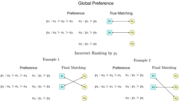
Figure 2: Examples of the matching result caused by the incorrect ranking provided by agent $p_{1}$ when agent $p_{2}$ submits the correct ranking list under the global preference. In Example 1, Agent $p_{1}$ provides an incorrect ranking $p_{1}:a_{2}>a_{1}>a_{3}$. Based on the GS algorithm, the final matching result is $\{(p_{1},a_{2}),(p_{2},a_{2})\}$. It creates a positive regret for both agents. In Example 2: Agent $p_{1}$ provides an incorrect ranking $p_{1}:a_{3}>a_{2}>a_{1}$. Based on the GS algorithm, the final matching result is $\{(p_{1},a_{3}),(p_{2},a_{2})\}$. It creates a positive regret for $p_{1}$ and no regret for $p_{2}$.

In the exploration stage, agent $p_{i}$’s regret is caused by matching with super-optimal $\mathcal{Q}_{i,\text{sup}}(t)$ arms and sub-optimal arms $\mathcal{Q}_{i,\text{sub}}(t)$, where the definition of super-optimal arms’ set and sub-optimal arms’ set can be found in Section 4.1. After the exploration stage stops, all agent rank arms based on estimated mean rewards from Eq. (5) in descending order. For agent $p_{i}$, this ranking list is denoted as $\hat{{\bm{\mathbf{{r}}}}}_{i,[K]}(t)$. However, some agents’ estimators are coarse due to the insufficient exploration, resulting in wrongly ranked arms. Here we present 6 matching status if $p_{1}$ wrongly estimates the ranking list and $p_{2}$ correctly estimates the ranking list as an example to illustrate the instantaneous regret’s classification, where the instantaneous regret’s classification will help us analyze the regret lower bound in the following step. This scenario will create six ($3!=6$) preference schemes based on the matching result in this two-agents three-arms two-sided competing matching market. We will show the details of these six cases as follows.

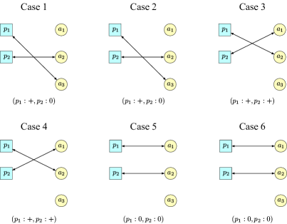
Figure 3: The corresponding matching results and regret status in six cases when agent $p_{1}$ submits an incorrect ranking. Single agent suffers regret: Case 1 and Case 2. Both agents suffer regret: Case 3 and Case 4. No regret: Case 5 and Case 6.

Case 1 (Single Agent Suffers Regret). If $p_{1}$ wrongly estimates the ranking preference over arm as $p_{1}:a_{3}>a_{1}>a_{2}$, the matching result by GS algorithm is shown in Figure 3 Case 1. $p_{1}$ is matched with $a_{3}$ and $p_{2}$ is matched with $a_{2}$. In this case, $p_{1}$ suffers regret but $p_{2}$ does not.

Case 2 (Single Agent Suffers Regret). If $p_{1}$ wrongly estimates the ranking preference over arm as $p_{1}:a_{3}>a_{2}>a_{1}$, the matching result by GS algorithm is shown in Figure 3 Case 2. $p_{1}$ is matched with $a_{3}$ and $p_{2}$ is matched with $a_{2}$. The regret status is the same as Case 1.

Case 3 (Both Agents Suffer Regret). If $p_{1}$ wrongly estimates the ranking preference over arm as $p_{1}:a_{2}>a_{3}>a_{1}$, the matching result by GS algorithm is shown in Figure 3 Case 3. $p_{1}$ is matched with $a_{2}$ and $p_{2}$ is matched with $a_{1}$. Now $p_{1}$ suffers a positive regret since $p_{1}$’s optimal matching objective is $a_{1}$ and $p_{2}$ suffers a positive regret since $p_{2}$’s stable optimal matching objective is $a_{2}$.

Case 4 (Both Agents Suffer Regret). If $p_{1}$ wrongly estimates the ranking preference over arm as $p_{1}:a_{2}>a_{1}>a_{3}$, the matching result by GS algorithm is shown in Figure 3 Case 4. $p_{1}$ is matched with $a_{2}$ and $p_{2}$ is matched with $a_{1}$. The regret is the same as Case 3.

Case 5 (No Regret). If $p_{1}$ wrongly estimates the ranking preference over arm as $p_{1}:a_{1}>a_{3}>a_{2}$, the matching result by GS algorithm is shown in Figure 3 Case 5. $p_{1}$ is matched with $a_{1}$ and $p_{2}$ is matched with $a_{2}$. Although agent $p_{i}$ wrongly sorts arms $a_{1}$ and $a_{2}$, the matching result is correct and no agent suffers regret.

Case 6 (No Regret). If $p_{1}$ correctly estimates the ranking preference over arm as $p_{1}:a_{1}>a_{2}>a_{3}$, the matching result by GS algorithm is shown in Figure 3 Case 6. $p_{1}$ is matched with $a_{1}$ and $p_{2}$ is matched with $a_{2}$. Here the agent $p_{1}$ correctly sorts its preference and no agent suffers regret. The final regret performance is the same as Case 5.

For agent $p_{1}$, the four regret-occurred cases are represented in Case 1 to Case 4. The two regret-vanished cases happen in Case 5 and Case 6. For agent $p_{2}$, the two regret-occurred cases are represented in Case 3 and Case 4. The four regret-vanishing cases happen in Case 1, Case 2, Case 5, and Case 6. These six cases represent all the possible regret occurring cases when $p_{1}$ submits incorrect ranking and $p_{2}$ submits correct ranking. Based on these 6 matching status, we find that even when the submitted ranking is not correct, there will be no regret for both agent $p_{1}$ and agent $p_{2}$. However, this status is not a stabilized point. As long as any agent deviate this status, there is no guarantee that both agents will be back to this status. The true stable matching result is a stabilized point since there is no blocking pair. The detailed instantaneous regret result decomposition for these six cases can be found in the supplementary material.

6 Simulation

In this section, we demonstrate the effectiveness and robustness of CC-ETC in five different settings. In the simulation study, CC-ETC demonstrates its robustness under different context distributions (S1 $\&$ S2), different minimal margins (S3), and additional experiments such as different feature vector dimensions (S4) and different sizes of agents and arms (S5) are available in Appendix Section A8 .

6.1 Data Generation and Hyperparameter Setting

From Scenario 1 to Scenario 4, we consider that there are two agents $\mathcal{N}=\{p_{1},p_{2}\}$ and three arms $\mathcal{K}=\{a_{1},a_{2},a_{3}\}$. In Scenario 5, we consider that there are five agents and five arms. The ridge parameters for all agents are set to be $\lambda=0.1$ in all scenarios. Besides, since the exploration length $\overline{h}_{i}$ is usually not the multiple of $\binom{K}{N}$, we round $\overline{h}_{i}$ to the closet multiple of $\binom{K}{N}$. Finally, we set $\overline{h}$ as the the largest exploration length, $\overline{h}=\underset{i\in[N]}{\max}\;\overline{h}_{i}$. Here we assume $\sigma$ is known.

Scenario 1 (S1): The time horizon is set to be $T=1000$. The contextual features are all generated from a two-dimensional multivariate normal distribution. For arms $a_{1},a_{2},a_{3}$, their contexts are randomly generated as follows ${\bm{\mathbf{{x}}}}_{1}(t)\sim N(\mu_{1},\zeta{\bm{\mathbf{{I}}}}_{2})),\text{with }\mu_{1}=(0.667,0.745)^{\sf T},{\bm{\mathbf{{x}}}}_{2}(t)\sim N(\mu_{2},\zeta{\bm{\mathbf{{I}}}}_{2})),\text{with }\mu_{2}=(0.745,0.667)^{\sf T},{\bm{\mathbf{{x}}}}_{3}(t)\sim N(\mu_{3},\zeta{\bm{\mathbf{{I}}}}_{2})),\text{with }\mu_{3}=(0.994,0.110)^{\sf T}$. The true parameters for two agents are randomly generated as ${\bm{\mathbf{{\theta}}}}_{1,*}=(0.530,0.848)^{\sf T},{\bm{\mathbf{{\theta}}}}_{2,*}=(0.894,0.447)^{\sf T}.$ Note that these mean values $\mu_{1},\mu_{2},\mu_{3}$ are all randomly generated and then normalized to have a unit norm. Contexts features are all normalized after being sampled from these normal distributions. This setup allows us to focus on the effect of the similarity rather than the effect of contexts’ magnitude (norm of contexts). This, in fact, makes the problem harder, which means agents will focus on the similarity rather the magnitude. We set the fluctuation variance with four levels $\zeta=[0.01,0.05,0.1,0.2]$. The true parameters in the linear reward model in Eq. (1) are also random generated (See Supplmentary material). The values of $\theta_{1,*}$ and $\theta_{2,*}$ are again randomly generated and then normalized so that their norms are one. In addition, the noise is generated from normal distribution $\epsilon_{i,j}(t)\sim N(0,\sigma),\forall i\in[N],j\in[K],t\in[T]$ and the noise level is $\sigma=0.05$. We assume that arms to agents’ preference is the non-global preference, $a_{1}:p_{1}>p_{2},a_{2}:p_{2}>p_{1},a_{3}:p_{1}>p_{2}$, which is known to be much more difficult than the global preference setting. When contexts are fixed at $\mu_{1}$, $\mu_{2}$, and $\mu_{3}$, i.e, contexts have no noise, the true optimal matching at the static level is $\{(p_{1},a_{1}),(p_{2},a_{2})\}$. However, since contexts are noisy and shifting, the optimal matching also shifts over time. The uniform minimal margin condition for this scenario is set to be $\overline{\Delta}_{i,\min}=0.2,\forall i\in[N]$. According to Eq.(7), the exploration stage length $\overline{h}$ is 312.

Scenario 2 (S2): Different from S1, in S2 the contextual features move with an angular velocity $w_{t}=0.005t,t\in[T]$. Contextual features for arms $a_{1},a_{2},a_{3}$ are generated as, ${\bm{\mathbf{{x}}}}_{1}(t)\sim N(\mu_{1}(t),\zeta{\bm{\mathbf{{I}}}}_{2}),\text{with }\mu_{1}(t)=(0.667+w(t),0.745)^{\sf T},{\bm{\mathbf{{x}}}}_{2}(t)\sim N(\mu_{2},\zeta{\bm{\mathbf{{I}}}}_{2})),\text{with }\mu_{2}=(0.745,0.667)^{\sf T},{\bm{\mathbf{{x}}}}_{3}(t)\sim N(\mu_{3},\zeta{\bm{\mathbf{{I}}}}_{2})),\text{with }\mu_{3}=(0.994,0.110)^{\sf T},$ where $a_{2}$ and $a_{3}$’s contexts are the same as those in S1. The true parameters $\theta_{1,*},\theta_{2,*}$ are the same as these in S1. This moving context with an angular velocity is the same setting illustrated in Figure 1. We consider three levels of noise $\sigma=[0.01,0.02,0.05]$ to test the robustness of our algorithm. In this setting, the true mean agent-optimal matching is no longer fixed even when $\zeta=0$ since $\mu_{1}(t)$ is also constantly changing. The uniform minimal margin condition for this scenario is set to be $\overline{\Delta}_{i,\min}=0.2,\forall i\in[N]$. The exploration stage length $\overline{h}$ for the three noise levels are $\overline{h}=[24,66,312]$, correspondingly.

Scenario 3 (S3): The uniform minimal margin condition for this scenario is set to be $\overline{\Delta}_{i,\min}=0.05,\forall i\in[N]$. The time horizon is set to be $T=5000$ to have a long enough exploration length since we decrease the uniform minimal margin condition. The exploration length $\overline{h}$ for the three noise levels are $\overline{h}=[264,876,4014]$, correspondingly. Thus the difference between S3 and S2 is the time horizon $T$ and different hyperparameters. The data generation process for S3 and S2 are the same.

6.2 Results

In Figures 4, 5, 5, the horizontal axis represents the time point and the vertical axis represents the cumulative regret. In all figures, we plot the maximum (worst) regret represented as the upper bound shaded line, mean regret represented as the solid line, and minimum (best) regret represented as the lower bound shaded line, over 100 replications.

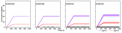
Figure 4: Cumulative regret for different context variation levels in Scenario S1. Each black stick means a change of optimal matching.

Scenario 1 (S1): CC-ETC is robust to different contexts’ variance levels. In Figure 4, our CC-ETC shows the logarithmic regret shape which demonstrates that it is robust to contexts’ noise levels. When contexts’ variance level $\zeta$ increases, the shaded area becomes wider, indicating the uncertainty of the regret increasing. In this figure and following figures, we use the short black sticks to represent the change of the optimal matching between two continuous-time points due to the contextual information change. We mark the short black stick at time $t+1$ on the horizontal axis if $\overline{{\bm{\mathbf{{m}}}}}(t)\neq\overline{{\bm{\mathbf{{m}}}}}(t+1)$, which means that the optimal matching result is different on two continuous-time points. The denser the black stick is, the more frequently the agent-optimal matching changes over time. In other words, when the contexts’ fluctuation magnitudes increase, the optimal stable matching changes more frequently, and it exhibits the dynamic property of COMBO.

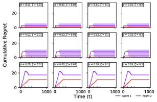
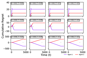
Figure 5: Left: Cumulative regret for different noise levels and context variation levels of mean shifting context in Scenario S2. Right: Cumulative regret for different noise levels and context variation levels in Scenario S3.

Scenario 2 (S2): CC-ETC is robust to mean shifting context distributions and different levels of observed score noise. In Figure 5, we present the S2’s results when the mean of arm $a_{1}$ changes with an angular velocity. In row 1, we find there is a small “bump” in the mean regret of the cumulative regret in each plot, and the slight bump occurs at the exploitation stage where the occurring time of the bump is greater than $\overline{h}$. Two reasons cause the occurrence of the small bump. One is the coarse estimation of parameters. Another is that the context’s angular velocity changes too slowly, violating the uniform minimal margin condition assumption. Both of these will cause the incorrect ranking list submitted by agents to the platform, which results in regret. A similar pattern can also be found in the second row of the figure. In order to demonstrate this, we decrease the uniform minimal margin condition $\overline{\Delta}_{i,\min}$ from 0.2 to 0.1 in S3 (in Figure 5), which indirectly extends the exploration stage and increases the estimation accuracy because agents can gather more data to get good estimates. In addition, in the third row, the shaded area disappears because the exploration stage is long enough to accumulate sufficient data to get a reasonable estimate compared with the first row and the second row. Another interesting finding is the decreasing regret phenomena after the bump. In the first row and the second row of the figure, the decreasing regret phenomena occur because the agent needs to recover from the violating “uniform minimal margin condition” assumption region for agent $p_{1}$. That means agent $p_{1}$ cannot distinguish the difference between arms when the true uniform minimal margin condition is less than that in Assumption 1. In the third row, the regret decreases over a long period because agent $p_{1}$ is in the exploration stage and the super-optimal arms have a much larger gain over sub-optimal arms. These significant gains will result in a negative regret. So the cumulative regret will decrease. This interesting phenomenon is only occurring in COMBO when considering the contextual information. In all, we find that CC-ETC is robust to changing the context format. Additional experiments settings and results are available in supplementary material.

Scenario 3 (S3): CC-ETC is robust to different uniform minimal margin scenarios. In Figure 5, we present the result of S3. As we change $\overline{\Delta}_{i,\min}=0.2$ in S2 to $\overline{\Delta}_{i,\min}=0.05,$ in S3 $\forall i\in[1,2]$, the exploration length becomes larger and the estimation becomes better. Compared with S2’s first row and second row, the shaded area in S3’s first row and second row becomes narrower, which substantiates our conjecture. In the second row and third row, we find that agent $p_{1}$ achieves the negative cumulative regret mainly because in the exploration stage, agent $p_{1}$ is periodically matched with the super-optimal arm with a huge (in absolute value) negative regret.

SUPPLEMENT TO “RATE-OPTIMAL CONTEXTUAL ONLINE MATCHING BANDIT”

This appendix is organized as follows. In Section A1, we provide the Bernstein concentration lemma and tail probability’s upper bound and lower bound for the normal distribution. In Section A2, the detail of the GS Algorithm 4 under the job application scenario is provided. In Section A3, we prove that if agents can submit valid rankings to the platform, agents will acquire the matching which is as least as good as the stable matching. In Section A4, we provide detailed proof of the regret upper bound of CC-ETC. In Section A5, the detailed instantaneous regret decomposition at time $t$ is available when we consider there are two agents and three arms in this online matching market. In Section A6, we show lemmas of the probability lower bound. Finally, we provide detailed proof of the instance-dependent regret lower bound in Section A7. In Section A8, we provide more experimental results of CC-ETC.

Appendix A1 Miscellaneous Lemmas

Lemma 1

(Bernstein Concentration). Let $\{D_{k},\mathcal{F}_{k}\}_{k=1}^{\infty}$ be a martingale difference, and suppose that $D_{k}$ is a $\sigma$-subgaussian in an adapted sense, i.e., for all $\alpha\in\mathbb{R}$. $\mathbb{E}[e^{\alpha D_{k}}|\mathcal{F}_{k-1}]\leq e^{\frac{\alpha^{2}\sigma^{2}}{2}}$ almost surely. Then, for all $t\geq 0$,

$$\mathbb{P}[|\sum_{k=1}^{n}D_{k}|\geq t]\leq 2e^{-\frac{t^{2}}{2n\sigma^{2}}}.$$ (C.1)

Lemma 1 is from Theorem 2.3 of Wainwright (2019) (Wainwright, 2019) when $\alpha_{\ast}=\alpha_{k}=0$ and $\nu_{k}=\sigma$ for all $k$.

Lemma 2

(Tails of Normal distribution). Let $g\sim N(0,1)$. Then for all $t>0$, we have

$$(\frac{1}{t}-\frac{1}{t^{3}})\frac{1}{\sqrt{2\pi}}e^{(-t^{2}/2)}\leq\mathbb{P}(g\geq t)\leq\frac{1}{t}\frac{1}{\sqrt{2\pi}}e^{(-t^{2}/2)}.$$ (C.2)

Appendix A2 Deferred Acceptance (also known GS) Algorithm

In this part, we present the DA algorithm in the example of job seeking scenario.

1 Input: Companies set $\mathcal{N}$, job applicants set $\mathcal{K}$, companies to job applicants’ preferences, job applicants to companies’ preferences.

2 Initialize: An empty set $S$.

3 while $\exists$ A company $p$ who is not matched and has not contacted to every job applicant do

4       Let $a$ be the highest ranking job applicant in company $p$’s preference, to whom company $p$ has not yet contacted.

5       Now company $p$ contacts the job applicant $a$.

6       if Job applicant $a$ is free then

7             $(p,a)$ become matched (add $(p,a)$ to $S$).

8            

9      else

10             Job applicant $a$ is matched to company $p^{\prime}$ (add $(p^{\prime},a)$ to $S$).

11             if Job applicant $a$ prefers company $p^{\prime}$ to company $p$ then

12                   Company $p$ remains free (remove ($p,a$) from $S$).

13                  

14            else

15                   Job applicant $a$ prefers company $p$ to company $p^{\prime}$.

16                   Company $p^{\prime}$ becomes free (remove ($p^{\prime},a$) from $S$).

17                   ($p,a$) are paired (add ($p,a$) to $S$).

18                  

19            

20      

Output: Matching result $S$.

Algorithm 4 GS Algorithm

Appendix A3 Proof of Invalid ranking

Lemma 3 states that if all agents can submit valid rankings to the platform, the GS-Algorithm will provide a matching ${\bm{\mathbf{{m}}}}(t)$ as least as good as $\overline{{\bm{\mathbf{{m}}}}}(t)$.

Lemma 3

If all agents submit valid rankings to the platform, then the GS-algorithm find a matching at each time step $t$, $m(t)$, such that $\mu_{i,m_{i}(t)}(t)\geq\mu_{i,\overline{m}_{i}(t)}(t)$ for all agents $p_{i}$.

Proof. First, we show that the agent-optimal matching $\overline{m}(t)$ is stable according to the rankings submitted by agents when all those rankings are valid.

Let $a_{j}$ be an arm such that $\hat{r}_{i,j}(t)<\hat{r}_{i,\overline{m}_{i}(t)}(t)$ for agent $p_{i}$. Since $\hat{{\bm{\mathbf{{r}}}}}_{i,[K]}(t)$ is valid, it means that $p_{i}$ prefers $a_{j}$ over $\overline{m}_{i}(t)$ according to the preference. However, since $\overline{m}(t)$ is stable according to the true preference, arm $a_{j}$ must prefer agent $\overline{m}_{j}(t)^{-1}$ over $p_{i}$ because arm $a_{j}$ has no incentive to deviate the current matching $\overline{m}(t)$, where $\overline{m}_{j}(t)^{-1}$ is $a_{j}$’s matching according to $\overline{m}(t)$ or the empty set if $a_{j}$ does not have a match. Therefore, according to the ranking $\hat{{\bm{\mathbf{{r}}}}}_{i,[K]}(t)$, $p_{i}$ has no incentive to deviate to arm $a_{j}$ because that arm $a_{j}$ would reject him.

Since $\overline{m}(t)$ is a stable matching according to rankings $\hat{{\bm{\mathbf{{r}}}}}_{i,[K]}(t)$, we know that the GS-algorithm will output a matching which is at least as good as $\overline{m}(t)$ for all agents according to rankings $\hat{r}_{i,j}$. Since all rankings are valid, it follows that the GS algorithm will output a matching $m(t)$ which is as least as good as $\overline{m}(t)$.

Appendix A4 Proof of Theorem 1 - Regret Upper Bound

A4.1 Regret Decomposition

In this section, we provide the regret decomposition and key steps to prove Theorem 1. We decompose the agent-wise regret $R_{i}(T)$ into the exploration stage regret and the exploitation stage regret as follows:

$$R_{i}(T) \equiv\sum_{t=1}^{T}\mu_{i,\overline{m}_{i}(t)}(t)-\sum_{t=1}^{T}\mu_{i,m_{i}(t)}(t)$$

$$\leq\underbrace{\sum_{t=1}^{\bar{h}}\overline{\Delta}_{i,m_{i}(t)}(t)}_{\text{Part I Regret}}+\underbrace{\Bigg{[}\sum_{t=\overline{h}+1}^{T}\overline{\Delta}_{i,\max}(t)(N\mathbb{P}(\hat{r}_{i,t}\text{ is invalid})}_{\text{Part II Regret}})\Bigg{]}.$$

As for the part I regret, the $\mu_{i,\overline{m}_{i}(t)}(t)-\mu_{i,m_{i}(t)}(t)$ is equal to $\overline{\Delta}_{i,m_{i}(t)}(t)$ by definition. As for the part II regret, we need to quantify when the matching result $m_{i}(t)$ produced by the CC-ETC for agent $p_{i}$ at time $t$ ($\geq\overline{h}+1$) is inferior than the agent-optimal matching result $\overline{m}_{i}(t)$, which causes a positive regret. Recall the definition of the maximum gap in Section 4.1. We always have $\mu_{i,\overline{m}_{i}(t)}(t)-\mu_{i,m_{i}(t)}(t)\leq\overline{\Delta}_{i,\max}(t)$. In order to describe when this regret occurs, we introduce the definition of the valid ranking and the invalid ranking.

Definition 1

Ranking $\hat{{\bm{\mathbf{{r}}}}}_{i,[K]}(t)$ is valid if whenever an arm $a_{j}$ is ranked higher than $\overline{m}_{i}(t)$, i.e, $\hat{r}_{i,j}(t)<\hat{r}_{i,\overline{m}_{i}(t)}(t)$, it follows that $\mu_{i,j}(t)>\mu_{i,\overline{m}_{i}(t)}(t)$. On the other hand, if an agent ranks arms with lower mean reward higher than the agent-optimal arm, then it is invalid.

The definition of the invalid ranking only requires the ranking of the sub-optimal arms are not ranked higher than the agent-optimal arms, rather than all arms are ranked correctly, which is a weak constraint over the estimated ranking provided by the agent.

With the definition of the valid ranking, Lemma 3 in the supplementary material shows that, if all agents submit valid rankings to the platform, the GS algorithm will provide a matching ${\bm{\mathbf{{m}}}}(t)$ as least as good as $\overline{{\bm{\mathbf{{m}}}}}(t)$ according to true preferences. Thus, there will be no positive regret. That means, if there exists one arm $a_{j}$ such that $\mu_{i,j}(t)<\mu_{i,\overline{m}_{i}(t)}(t)$, but $\hat{r}_{i,j}(t)<\hat{r}_{i,\overline{m}_{i}(t)}(t)$, it will cause a positive regret. So the instantaneous regret in the exploitation stage at each time step becomes $\Delta_{i,m_{i}(t)}(t)N\mathbb{P}(\hat{r}_{i,t}\text{ is invalid})$ which is less than $\Delta_{i,\max}(t)N\mathbb{P}(\hat{r}_{i,t}\text{ is invalid})$, where “$N$” here takes a union bound to get. The details of how to quantify the invalid ranking probability $\mathbb{P}(\hat{r}_{i,t}\text{ is invalid})$ can be found in Section A4.2. Then we sum over the instantaneous regret from time $\overline{h}+1$ to $T$ to get the “Part II Regret” as shown in Eq. (6). The overall regret can be obtained by adding the Part I regret and the Part II regret.

Part I regret can be easily obtained by calculating the regret between the assigned arm $m_{i}(t)$ and the agent-optimal arm $a_{\overline{m}_{i}(t)}$. We have the Part I regret as follows

$$\textit{Part I Regret}=\sum_{t=1}^{\bar{h}}\overline{\Delta}_{i,m_{i}(t)}(t),$$ (C.3)

where $\overline{\Delta}_{i,j}(t)=\mu_{i,\overline{m}_{i}(t)}(t)-\mu_{i,m_{i}(t)}(t)$ for $t\leq\overline{h}$.

The exploitation regret (Part II Regret) can be calculated as the product of the invalid ranking probability and the instantaneous regret over time $t>\overline{h}$. So we first provide the Lemma 4 to quantify the probability upper bound of the invalid ranking and the instantaneous regret in Section A4.3. Then we obtain the order of the regret upper bound of CC-ETC in Section A4.4.

A4.2 Invalid Ranking Lemma

The core step to getting part II’s regret at the exploitation stage is to decompose the instantaneous regret into the product of a bad event’s happening probability (invalid ranking probability) and its corresponding regret. By Lemma 3 in the supplementary material, if all agents can submit valid rankings to the platform, then no regret occurs. Thus, we focus on quantifying the invalid ranking probability.

Lemma 4

Assume Assumption 1 and Assumption 2 hold, if agent $p_{i}$ follows the CC-ETC algorithm, we have the invalid ranking probability’s upper bound at time $t\geq\overline{h}+1$,

$$\mathbb{P}(\hat{r}_{i,t}\text{ is invalid})\leq K\exp\Bigg{[}-\overline{h}\frac{\lambda_{i}^{2}\overline{\Delta}_{i,\min}^{2}}{2d^{2}{\bm{\mathbf{{x}}}}_{i,\max}^{2}\sigma^{2}}+\log(2d)\Bigg{]}.$$ (C.4)

The key step to evaluate the invalid ranking probability $\mathbb{P}(\hat{r}_{i,t}\text{ is invalid})$ is to consider the probability $\mathbb{P}(\hat{\mu}_{i,j}(t)>\hat{\mu}_{i,\overline{m}_{i}(t)}(t))$ where $\mu_{i,\overline{m}_{i}(t)}(t)>\mu_{i,j}(t)$, but $\hat{r}_{i,j}(t)<\hat{r}_{i,\overline{m}_{i}(t)}(t)$, based on the definition of the invalid ranking. Due to the linear structure of the reward, we find the invalid ranking probability can be upper bounded by the tail probability of the estimation error of the true preference parameter, $\mathbb{P}(\hat{r}_{i,t}\text{ is invalid})\leq\mathbb{P}\Big{[}\left\lVert\widehat{{\bm{\mathbf{{\theta}}}}}_{i}(\overline{h})-{\bm{\mathbf{{\theta}}}}_{i,*}\right\rVert_{2}\geq\langle{\bm{\mathbf{{\theta}}}}_{i,*},\frac{{\bm{\mathbf{{x}}}}_{\overline{m}_{i}(t)}(t)-{\bm{\mathbf{{x}}}}_{j}(t)}{\left\lVert{\bm{\mathbf{{x}}}}_{\overline{m}_{i}(t)}(t)-{\bm{\mathbf{{x}}}}_{j}(t)\right\rVert_{2}}\rangle\Big{]}$. Here we define similarity difference as follows,

$$\langle{\bm{\mathbf{{\theta}}}}_{i,*},\frac{{\bm{\mathbf{{x}}}}_{\overline{m}_{i}(t)}(t)-{\bm{\mathbf{{x}}}}_{j}(t)}{\left\lVert{\bm{\mathbf{{x}}}}_{\overline{m}_{i}(t)}(t)-{\bm{\mathbf{{x}}}}_{j}(t)\right\rVert_{2}}\rangle =\left\lVert{\bm{\mathbf{{\theta}}}}_{i,*}\right\rVert_{2}\langle\frac{{\bm{\mathbf{{\theta}}}}_{i,*}}{\left\lVert{\bm{\mathbf{{\theta}}}}_{i,*}\right\rVert_{2}},\frac{{\bm{\mathbf{{x}}}}_{\overline{m}_{i}(t)}(t)-{\bm{\mathbf{{x}}}}_{j}(t)}{\left\lVert{\bm{\mathbf{{x}}}}_{\overline{m}_{i}(t)}(t)-{\bm{\mathbf{{x}}}}_{j}(t)\right\rVert_{2}}\rangle\overset{\Delta}{=}\left\lVert{\bm{\mathbf{{\theta}}}}_{i,*}\right\rVert_{2}\cos({\phi_{i,j}(t)}),$$

where $\cos({\phi_{i,j}(t)})$ is the dynamic similarity score. $\phi_{i,j}(t)$ represents the angle between the normalized true parameter ${\bm{\mathbf{{\theta}}}}_{i,*}$ and the normalized arms difference at time step $t$. This angle $\phi_{i,j}(t)$ represents the similarity between the sub-optimal arm $a_{j}$ and agent-optimal arm $a_{\overline{m}_{i}(t)}$ from the viewpoint of agent $p_{i}$ at time $t$, which links to the chance of happening of submitting the invalid ranking. If the dynamic similarity score is small, it has a high chance for agent to submit invalid rankings.

Under Assumption 1, we assume there is no tie between the sub-optimal arm and the agent-optimal arm which is equivalent to exclude two potential sources, (1) no identical arms over time and (2) no symmetric arms at the viewpoint of ${\bm{\mathbf{{\theta}}}}_{i,*}$ over time. With Assumption 1, $\overline{\Delta}_{i,\min}=\underset{j\in[K]}{\min}\underset{t\in[T]}{\min}\left\lVert{\bm{\mathbf{{\theta}}}}_{i,*}\right\rVert_{2}\cos({\phi_{i,j}(t)})>0$, so $\{\left\lVert\widehat{{\bm{\mathbf{{\theta}}}}}_{i}(\overline{h})-{\bm{\mathbf{{\theta}}}}_{i,*}\right\rVert_{2}\geq\langle{\bm{\mathbf{{\theta}}}}_{i,*},\frac{{\bm{\mathbf{{x}}}}_{\overline{m}_{i}(t)}(t)-{\bm{\mathbf{{x}}}}_{j}(t)}{\left\lVert{\bm{\mathbf{{x}}}}_{\overline{m}_{i}(t)}(t)-{\bm{\mathbf{{x}}}}_{j}(t)\right\rVert_{2}}\rangle\}\subset\{\left\lVert\widehat{{\bm{\mathbf{{\theta}}}}}_{i}(\overline{h})-{\bm{\mathbf{{\theta}}}}_{i,*}\right\rVert_{2}\geq\overline{\Delta}_{i,\min}\}.$ That is, if we want to measure the chance of happening of submitting the invalid ranking, we need to quantify the tail probability of the statistical error of the ridge estimator $\mathbb{P}[\left\lVert\widehat{{\bm{\mathbf{{\theta}}}}}_{i}(\overline{h})-{\bm{\mathbf{{\theta}}}}_{i,*}\right\rVert_{2}\geq\overline{\Delta}_{i,\min}]$. Finally, based on Lemma EC.7.2 from (Bastani and Bayati, 2020), we get the invalid ranking probability’s upper bound, $\mathbb{P}[\left\lVert\widehat{{\bm{\mathbf{{\theta}}}}}_{i}(\overline{h})-{\bm{\mathbf{{\theta}}}}_{i,*}\right\rVert_{2}\geq\overline{\Delta}_{i,\min}]\leq\exp[-\overline{h}\frac{\lambda_{i}^{2}\overline{\Delta}_{i,\min}^{2}}{2d^{2}{\bm{\mathbf{{x}}}}_{i,\max}^{2}\sigma^{2}}+\log(2d)]$. Because we need to consider all such sub-optimal arms $\mathcal{Q}_{i,\text{sub}}(t)$, the following inequality provides the uniform upper bound of the invalid ranking probability, $\mathbb{P}(\hat{{\bm{\mathbf{{r}}}}}_{i,[K]}(t)\text{ is invalid})\leq K\exp\bigg{[}-\overline{h}\frac{\lambda_{i}^{2}\overline{\Delta}_{i,\min}^{2}}{2d^{2}{\bm{\mathbf{{x}}}}_{i,\max}^{2}\sigma^{2}}+\log(2d)\bigg{]}$, with $|\mathcal{Q}_{i,\text{sub}}(t)|\leq K$, which completes key steps of the proof.

With the above invalid ranking probability upper bound, the regret for agent $p_{i}$ at the exploitation stage can be upper bounded by $\overline{\Delta}_{i,\max}(t)\mathbb{P}(\hat{{\bm{\mathbf{{r}}}}}_{i,[K]}(t)\text{ is invalid})\leq\overline{\Delta}_{i,\max}(t)\times NK\exp\bigg{[}-\overline{h}\frac{\lambda_{i}^{2}\overline{\Delta}_{i,\min}^{2}}{2d^{2}{\bm{\mathbf{{x}}}}_{i,\max}^{2}\sigma^{2}}+\log(2d)\bigg{]}$. When we sum the above time-dependent regret over time $t$, we obtain the regret upper bound shown in Eq. (6).

A4.3 Proof of Lemma 4

Proof. We consider one specific time step $t$ at the exploitation stage throughout this proof. We next show how to quantify the invalid ranking probability.

In order to make the ranking $\hat{{\bm{\mathbf{{r}}}}}_{i,[K]}(t)$ to be invalid, there must exist an arm $a_{j}$ where $j\neq\overline{m}_{i}(t)$ such that $\mu_{i,\overline{m}_{i}(t)}(t)>\mu_{i,j}(t)$, but $\hat{r}_{i,j}(t)<\hat{r}_{i,\overline{m}_{i}(t)}(t)$, due to the coarse estimation of the true parameter. It means that $\hat{\mu}_{i,j}(t)>\hat{\mu}_{i,\overline{m}_{i}(t)}(t)$. The probability of this invalid ranking is equal to

$$\mathbb{P}(\hat{\mu}_{i,j}(t)>\hat{\mu}_{i,\overline{m}_{i}(t)}(t))$$ (C.5)

$$=\mathbb{P}\Big{[}\hat{\mu}_{i,j}(t)-\mu_{i,j}(t)-\hat{\mu}_{i,\overline{m}_{i}(t)}(t)+\mu_{i,\overline{m}_{i}(t)}(t)\geq\mu_{i,\overline{m}_{i}(t)}(t)-\mu_{i,j}(t)\Big{]}.$$

Based on the linear structure of the reward and the contextual information from Eq (1), we decompose $\mu_{i,j}(t)={\bm{\mathbf{{\theta}}}}_{i,*}^{\sf T}{\bm{\mathbf{{x}}}}_{j}(t)$ as defined in Eq. (5). The invalid ranking probability can be rewritten as

$$=\mathbb{P}\Big{[}\widehat{{\bm{\mathbf{{\theta}}}}}_{i}(\overline{h})^{\sf T}{\bm{\mathbf{{x}}}}_{j}(t)-{\bm{\mathbf{{\theta}}}}_{i,*}^{\sf T}{\bm{\mathbf{{x}}}}_{j}(t)-\widehat{{\bm{\mathbf{{\theta}}}}}_{i}(\overline{h})^{\sf T}{\bm{\mathbf{{x}}}}_{\overline{m}_{i}(t)}(t)+{\bm{\mathbf{{\theta}}}}_{i,*}^{\sf T}{\bm{\mathbf{{x}}}}_{\overline{m}_{i}(t)}(t)\geq\mu_{i,\overline{m}_{i}(t)}(t)-\mu_{i,j}(t)\Big{]}$$ (C.6)

$$=\mathbb{P}\Big{[}(\widehat{{\bm{\mathbf{{\theta}}}}}_{i}(\overline{h})-{\bm{\mathbf{{\theta}}}}_{i,*})^{\sf T}({\bm{\mathbf{{x}}}}_{j}(t)-{\bm{\mathbf{{x}}}}_{\overline{m}_{i}(t)}(t))\geq{\bm{\mathbf{{\theta}}}}_{i,*}^{\sf T}({\bm{\mathbf{{x}}}}_{\overline{m}_{i}(t)}(t)-{\bm{\mathbf{{x}}}}_{j}(t))\Big{]},$$

where we denote $\overline{\Delta}_{i,j}(t)=\mu_{i,\overline{m}_{i}(t)}(t)-\mu_{i,j}(t)={\bm{\mathbf{{\theta}}}}_{i,*}^{\sf T}({\bm{\mathbf{{x}}}}_{\overline{m}_{i}(t)}(t)-{\bm{\mathbf{{x}}}}_{j}(t))$. Besides, we define $\overline{\Delta}_{i,\min}(t)=\underset{j:\overline{\Delta}_{i,j}(t)>0}{\min}\overline{\Delta}_{i,j}(t)=\underset{j:\overline{\Delta}_{i,j}(t)>0}{\min}[\mu_{i,\overline{m}_{i}(t)}(t)-\mu_{i,j}(t)]$ as the minimum sub-optimal gap for agent $p_{i}$ at time step $t$, where the minimum sub-optimal gap $\overline{\Delta}_{i,\min}(t)$ for agent $p_{i}$ at time step $t$ represents the gap between the agent-optimal arm and the closest sub-optimal arm to the agent-optimal arm. So

$$\mathbb{P}(\hat{\mu}_{i,j}(t)>\hat{\mu}_{i,\overline{m}_{i}(t)}(t))$$ (C.7)

$$=\mathbb{P}\Big{[}(\widehat{{\bm{\mathbf{{\theta}}}}}_{i}(\overline{h})-{\bm{\mathbf{{\theta}}}}_{i,*})^{\sf T}({\bm{\mathbf{{x}}}}_{j}(t)-{\bm{\mathbf{{x}}}}_{\overline{m}_{i}(t)}(t))\geq{\bm{\mathbf{{\theta}}}}_{i,*}^{\sf T}({\bm{\mathbf{{x}}}}_{\overline{m}_{i}(t)}(t)-{\bm{\mathbf{{x}}}}_{j}(t))\Big{]}$$

$$\leq\mathbb{P}\Big{[}\left\lVert\widehat{{\bm{\mathbf{{\theta}}}}}_{i}(\overline{h})-{\bm{\mathbf{{\theta}}}}_{i,*}\right\rVert_{2}\left\lVert{\bm{\mathbf{{x}}}}_{j}(t)-{\bm{\mathbf{{x}}}}_{\overline{m}_{i}(t)}(t)\right\rVert_{2}\geq{\bm{\mathbf{{\theta}}}}_{i,*}^{\sf T}({\bm{\mathbf{{x}}}}_{\overline{m}_{i}(t)}(t)-{\bm{\mathbf{{x}}}}_{j}(t))\Big{]}$$

$$=\mathbb{P}\Big{[}\left\lVert\widehat{{\bm{\mathbf{{\theta}}}}}_{i}(\overline{h})-{\bm{\mathbf{{\theta}}}}_{i,*}\right\rVert_{2}\geq\langle{\bm{\mathbf{{\theta}}}}_{i,*},\frac{{\bm{\mathbf{{x}}}}_{\overline{m}_{i}(t)}(t)-{\bm{\mathbf{{x}}}}_{j}(t)}{\left\lVert{\bm{\mathbf{{x}}}}_{\overline{m}_{i}(t)}(t)-{\bm{\mathbf{{x}}}}_{j}(t)\right\rVert_{2}}\rangle\Big{]},$$

Where in the inequality, we use the Cauchy inequality to upper bound the left inner product. Here we find an interesting term called, similarity difference (SD), which is

SD $$\overset{\Delta}{=}\langle{\bm{\mathbf{{\theta}}}}_{i,*},\frac{{\bm{\mathbf{{x}}}}_{\overline{m}_{i}(t)}(t)-{\bm{\mathbf{{x}}}}_{j}(t)}{\left\lVert{\bm{\mathbf{{x}}}}_{\overline{m}_{i}(t)}(t)-{\bm{\mathbf{{x}}}}_{j}(t)\right\rVert_{2}}\rangle$$ (C.8)

$$=\left\lVert{\bm{\mathbf{{\theta}}}}_{i,*}\right\rVert_{2}\langle\frac{{\bm{\mathbf{{\theta}}}}_{i,*}}{\left\lVert{\bm{\mathbf{{\theta}}}}_{i,*}\right\rVert_{2}},\frac{{\bm{\mathbf{{x}}}}_{\overline{m}_{i}(t)}(t)-{\bm{\mathbf{{x}}}}_{j}(t)}{\left\lVert{\bm{\mathbf{{x}}}}_{\overline{m}_{i}(t)}(t)-{\bm{\mathbf{{x}}}}_{j}(t)\right\rVert_{2}}\rangle$$

$$=\left\lVert{\bm{\mathbf{{\theta}}}}_{i,*}\right\rVert_{2}\cos({\phi_{i,j}(t)}),$$

where $\phi_{i,j}(t)$ represents the angle between the normalized true parameter ${\bm{\mathbf{{\theta}}}}_{i,*}$ and the normalized arms difference at time step $t$, which is the similarity difference between arm $a_{j}$ and arm $a_{\overline{m}_{i}(t)}$ from the viewpoint of agent $p_{i}$.

Here we discuss the boundary scenario of the similarity difference. If SD = 0, there are three possible reasons.

• The first possible reason is that if the true parameter ${\bm{\mathbf{{\theta}}}}_{i,*}=0$. Since we assume all agents’ true parameters are meaningful and positive, with Assumption 2, we can rule out this case.

• The second possible reason is that if arm $a_{j}$ and arm $a_{\overline{m}_{i}(t)}$ are identical such that $x_{j}(t)=x_{\overline{m}_{i}(t)}$. Since we assume all arms are different, we can also rule out this case.

• The third possible reason is that if $\cos({\phi_{i,j}(t)})=0$. That means from the view point of agent $p_{i}$ at time $t$, arm $a_{j}$ and arm $a_{\overline{m}_{i}(t)}$ are symmetric. In other words, with our running example, company can not distinguish two job applicants $a_{j}$ and $a_{\overline{m}_{i}(t)}$ because they have different skills but the overall evaluation is the same, which is detailed illustrated in Section 4.1.

In order to avoid the last case, we introduce Assumption 1 where we assume that the uniform minimal margin condition over time is greater than zero. That means there is no symmetric case for the agent to distinguish two arms between the agent-optimal and the sub-optimal arm—That is the key difference between the COMBO and the MAB competing bandit problem. The MAB competing bandit only has one constant gap over time and no existence of the interesting symmetric arms. We now restate the uniform minimal margin condition $\overline{\Delta}_{i,\min}$ for agent $p_{i}$ over time $t$, that is $\overline{\Delta}_{i,\min}=\underset{j\in[K],t\in[T]}{\min}\left\lVert{\bm{\mathbf{{\theta}}}}_{i,*}\right\rVert_{2}\cos({\phi_{i,j}(t)})>0$.

If Assumption 1 holds, we consider the estimation error of the true parameter is lower bounded by the uniform minimal margin condition $\overline{\Delta}_{i,\min}$. So the probability of the invalid ranking is upper bounded by

$$=\mathbb{P}\Bigg{[}\left\lVert\widehat{{\bm{\mathbf{{\theta}}}}}_{i}(\overline{h})-{\bm{\mathbf{{\theta}}}}_{i,*}\right\rVert_{2}\geq\left\lVert{\bm{\mathbf{{\theta}}}}_{i,*}\right\rVert_{2}\cos({\phi_{i,j}(t)})\Bigg{]}$$ (C.9)

$$\leq\mathbb{P}\Bigg{[}\left\lVert\widehat{{\bm{\mathbf{{\theta}}}}}_{i}(\overline{h})-{\bm{\mathbf{{\theta}}}}_{i,*}\right\rVert_{2}\geq\overline{\Delta}_{i,\min}\Bigg{]}.$$

To get the upper bound of this tail event’s probability, we use the technique of quantifying the confidence ellipsoid from (Li et al., 2021). Notation $\hat{\Sigma}({\bm{\mathbf{{X}}}}_{i}(t))$ represents the normalized covariance matrix, so $\hat{\Sigma}({\bm{\mathbf{{X}}}}_{i}(t))=\Phi_{i}(t)/t=({\bm{\mathbf{{X}}}}_{i}(t)^{\sf T}{\bm{\mathbf{{X}}}}_{i}(t)+\lambda_{i}{\bm{\mathbf{{I}}}}_{d})/t$ for $t\geq 1$, where we define $\Phi_{i}(0)=\lambda_{i}{\bm{\mathbf{{I}}}}_{d}$ and $\lambda_{i}$ is the prespecified ridge hyperparameter for agent $p_{i}$. Note that the event $\lambda_{\min}(\hat{\Sigma}({\bm{\mathbf{{X}}}}_{i}(t)))>\lambda_{i}$ holds for $t\geq 1$. Thus after the exploration stage, agents have already gathered length $\overline{h}$ historical data, which include actions, rewards and contexts. So we have

$$\left\lVert\widehat{{\bm{\mathbf{{\theta}}}}}_{i}(\overline{h})-{\bm{\mathbf{{\theta}}}}_{i,*}\right\rVert_{2}$$ (C.10)

$$=\left\lVert({\bm{\mathbf{{X}}}}_{i}(\overline{h})^{\sf T}{\bm{\mathbf{{X}}}}_{i}(\overline{h})+\lambda_{i}{\bm{\mathbf{{I}}}})^{-1}{\bm{\mathbf{{X}}}}_{i}(\overline{h})^{\sf T}({\bm{\mathbf{{X}}}}_{i}(\overline{h}){\bm{\mathbf{{\theta}}}}_{i,*}+\epsilon)-{\bm{\mathbf{{\theta}}}}_{i,*}\right\rVert_{2}$$

$$=\left\lVert({\bm{\mathbf{{X}}}}_{i}(\overline{h})^{\sf T}{\bm{\mathbf{{X}}}}_{i}(\overline{h})+\lambda_{i}{\bm{\mathbf{{I}}}})^{-1}{\bm{\mathbf{{X}}}}_{i}(\overline{h})^{\sf T}\epsilon+{\bm{\mathbf{{\theta}}}}_{i,*}-\lambda_{i}({\bm{\mathbf{{X}}}}_{i}(\overline{h})^{\sf T}{\bm{\mathbf{{X}}}}_{i}(\overline{h})+\lambda_{i}{\bm{\mathbf{{I}}}})^{-1}{\bm{\mathbf{{\theta}}}}_{i,*}-{\bm{\mathbf{{\theta}}}}_{i,*}\right\rVert_{2}$$

$$=\left\lVert({\bm{\mathbf{{X}}}}_{i}(\overline{h})^{\sf T}{\bm{\mathbf{{X}}}}_{i}(\overline{h}))^{-1}({\bm{\mathbf{{X}}}}_{i}(\overline{h})^{\sf T}\epsilon-\lambda_{i}{\bm{\mathbf{{\theta}}}}_{i,*})\right\rVert_{2}$$

$$\leq\frac{1}{\overline{h}\lambda_{i}}\left\lVert{\bm{\mathbf{{X}}}}_{i}(\overline{h})^{\sf T}\epsilon-\lambda_{i}{\bm{\mathbf{{\theta}}}}_{i,*}\right\rVert_{2}.$$

Here we use a constant $\chi$ to represent the uniform minimal margin condition to get the estimation error. So we have

$$\text{Pr}\left[\left\lVert\widehat{{\bm{\mathbf{{\theta}}}}}_{i}(\overline{h})-{\bm{\mathbf{{\theta}}}}_{i,*}\right\rVert_{2}\leq\chi\right]$$ (C.11)

$$\geq\text{Pr}\left[(\left\lVert{\bm{\mathbf{{X}}}}_{i}(\overline{h})^{\sf T}\epsilon-\lambda_{i}{\bm{\mathbf{{\theta}}}}_{i,*}\right\rVert_{2}\leq\overline{h}\chi\lambda_{i})\cap(\lambda_{\min}(\hat{\Sigma}({\bm{\mathbf{{X}}}}_{i}(\overline{h}))>\lambda_{i})\right]$$

$$\geq 1-\sum_{r=1}^{d}\text{Pr}\left[|\epsilon^{\sf T}{\bm{\mathbf{{X}}}}^{(r)}_{i}(\overline{h})|>\lambda_{i}{\bm{\mathbf{{\theta}}}}_{i,*}^{(r)}+\frac{\overline{h}\chi\lambda_{i}}{\sqrt{d}}\right]-\text{Pr}\left[\lambda_{\min}(\hat{\Sigma}({\bm{\mathbf{{X}}}}_{i}(\overline{h}))\leq\lambda_{i})\right]$$

where we let ${\bm{\mathbf{{X}}}}^{(r)}_{i}(t)$ denote the $r^{\text{th}}$ column of ${\bm{\mathbf{{X}}}}_{i}(t)$. We can expand $\epsilon^{\sf T}{\bm{\mathbf{{X}}}}^{(r)}_{i}(t)=\sum_{j\in[t]}\epsilon(j){\bm{\mathbf{{x}}}}_{i,j}^{(r)}$, where we note that $D_{i,j,r}\equiv\epsilon(k){\bm{\mathbf{{x}}}}_{i,j}^{(r)}$ is a ${\bm{\mathbf{{x}}}}_{i,\max}\sigma$-subgaussian random variable, where ${\bm{\mathbf{{x}}}}_{i,\max}=\left\lVert{\bm{\mathbf{{X}}}}_{i}(t)\right\rVert_{\infty}$, conditioned on the sigma algebra $\mathcal{F}_{j-1}$ that is generated by random variable $X_{1},...,X_{j-1},Y_{1},...,Y_{j-1}$. Defining $D_{i,0,r}=0$, the sequence $D_{i,0,r},D_{i,1,r},...,D_{(i,j,r)}$ is a martingale difference sequence adapted to the filtration $\mathcal{F}_{1}\subset\mathcal{F}_{2}\subset...\mathcal{F}_{j}$ since $E[\epsilon(j){\bm{\mathbf{{x}}}}_{j}^{(r)}|\mathcal{F}_{j-1}]=0$. Using Lemma 1,

$$\text{Pr}\left[\left\lVert\widehat{{\bm{\mathbf{{\theta}}}}}_{i}(\overline{h})-{\bm{\mathbf{{\theta}}}}_{i,*}\right\rVert_{2}\leq\chi\right]$$ (C.12)

$$\geq 1-\sum_{r=1}^{d}\text{Pr}\left[|\epsilon^{\sf T}{\bm{\mathbf{{X}}}}^{(r)}_{i}(\overline{h})|>\lambda_{i}{\bm{\mathbf{{\theta}}}}_{i,*}^{(r)}+\frac{\overline{h}\chi\lambda_{i}}{\sqrt{d}}\right]-\text{Pr}\left[\lambda_{\min}(\hat{\Sigma}({\bm{\mathbf{{X}}}}_{i}(\overline{h}))\leq\lambda_{i})\right]$$

$$\geq 1-\sum_{r=1}^{d}\text{Pr}\left[|\epsilon^{\sf T}{\bm{\mathbf{{X}}}}^{(r)}_{i}(\overline{h})|>\frac{\overline{h}\chi\lambda_{i}}{\sqrt{d}}\right]-\text{Pr}\left[\lambda_{\min}(\hat{\Sigma}({\bm{\mathbf{{X}}}}_{i}(\overline{h}))\leq\lambda_{i})\right]$$

$$\geq 1-2d\exp{\left[-\frac{\overline{h}\chi^{2}\lambda_{i}^{2}}{2d\left\lVert{\bm{\mathbf{{X}}}}_{i}(\overline{h})\right\rVert_{\infty}^{2}\sigma^{2}}\right]}-\text{Pr}\left[\lambda_{\min}(\hat{\Sigma}({\bm{\mathbf{{X}}}}_{i}(\overline{h}))\leq\lambda_{i})\right],$$

where in the second inequality, we utilize the Case B1.2 in Lemma B.1 from (Li et al., 2021) since we assume all true parameters are positive ${\bm{\mathbf{{\theta}}}}_{i,*}^{(r)},\forall r\in[d],i\in[N]$ by Assumption 2. So we have the probability upper bound for the estimation error for any constant $\chi>0$,

$$\text{Pr}\left[\left\lVert\widehat{{\bm{\mathbf{{\theta}}}}}_{i}(\overline{h})-{\bm{\mathbf{{\theta}}}}_{i,*}\right\rVert_{2}\geq\chi\right]$$ (C.13)

$$\leq 2d\exp{\left[-\frac{\overline{h}\chi^{2}\lambda_{i}^{2}}{2d\left\lVert{\bm{\mathbf{{X}}}}_{i}(\overline{h})\right\rVert_{\infty}^{2}\sigma^{2}}\right]}-\text{Pr}\left[\lambda_{\min}(\hat{\Sigma}({\bm{\mathbf{{X}}}}_{i}(\overline{h}))\leq\lambda_{i})\right].$$

Since the event $\lambda_{\text{min}}(\Phi_{i}(\overline{h})/\overline{h})>\lambda_{i}>0$ holds by the requirement of condition, then $\text{Pr}\left[\lambda_{\min}(\hat{\Sigma}({\bm{\mathbf{{X}}}}_{i}(\overline{h}))\leq\lambda_{i})\right]=0$. Now we substitute $\chi=\overline{\Delta}_{i,\min}$ and get the following upper bound of the invalid ranking probability,

$$\mathbb{P}\Big{[}\left\lVert\widehat{{\bm{\mathbf{{\theta}}}}}_{i}(\overline{h})-{\bm{\mathbf{{\theta}}}}_{i,*}\right\rVert_{2}\geq\overline{\Delta}_{i,\min}\Big{]}$$ (C.14)

$$\leq\exp\Bigg{[}-\overline{h}\frac{\lambda_{i}^{2}\overline{\Delta}_{i,\min}^{2}}{2d^{2}{\bm{\mathbf{{x}}}}_{i,\max}^{2}\sigma^{2}}+\log(2d)\Bigg{]}-\mathbb{P}\Big{[}\lambda_{\min}(\hat{\Sigma}({\bm{\mathbf{{X}}}}_{i}(\overline{h}))\leq\lambda_{i}\Big{]}$$

$$=\exp\Bigg{[}-\overline{h}\frac{\lambda_{i}^{2}\overline{\Delta}_{i,\min}^{2}}{2d^{2}{\bm{\mathbf{{x}}}}_{i,\max}^{2}\sigma^{2}}+\log(2d)\Bigg{]}.$$

So the invalid ranking’s probability created by agent $p_{i}$ at time $t$ is upper bounded by

$$\mathbb{P}(\hat{\mu}_{i,j}(t)>\hat{\mu}_{i,\overline{m}_{i}(t)}(t))\leq\exp\Bigg{[}-\overline{h}\frac{\lambda_{i}^{2}\overline{\Delta}_{i,\min}^{2}}{2d^{2}{\bm{\mathbf{{x}}}}_{i,\max}^{2}\sigma^{2}}+\log(2d)\Bigg{]},$$ (C.15)

and because we consider all such sub-optimal arms $a_{j}$, we have the following uniform upper bound of the invalid ranking probability,

$$\mathbb{P}(\hat{{\bm{\mathbf{{r}}}}}_{i,[K]}(t)\text{ is invalid})\leq K\exp\Bigg{[}-\overline{h}\frac{\lambda_{i}^{2}\overline{\Delta}_{i,\min}^{2}}{2d^{2}{\bm{\mathbf{{x}}}}_{i,\max}^{2}\sigma^{2}}+\log(2d)\Bigg{]}.$$ (C.16)

With Lemma 4, we can quantify the regret at $t>\overline{h}$. So the instantaneous regret for agent $p_{i}$ at time $t$ will be upper bounded by

$$R_{i,t} \overset{\Delta}{=}\overline{\Delta}_{i,j}(t)\mathbb{P}(\text{at least one }\hat{{\bm{\mathbf{{r}}}}}_{i,[K]}(t)\text{ is invalid},\forall i\in[N])$$ (C.17)

$$\leq NK\overline{\Delta}_{i,\max}(t)\mathbb{P}(\hat{{\bm{\mathbf{{r}}}}}_{i,[K]}(t)\text{ is invalid}),$$

where we define $R_{i,t}$ as the instantaneous regret for agent $p_{i}$ at time $t$, $\overline{\Delta}_{i,\max}(t)=\underset{j}{\max}\overline{\Delta}_{i,j}(t)$ and $\overline{\Delta}_{i,\max}=\underset{t}{\max}\overline{\Delta}_{i,\max}(t)$. So similar to the standard analysis of ETC, we add the part I regret and part II regret together and get the regret upper bound of CC-ETC.

$$R_{i}(n) \leq\sum_{t=1}^{\bar{h}}\overline{\Delta}_{i,j}(t)+NK\Bigg{[}\sum_{t=\overline{h}+1}^{T}\overline{\Delta}_{i,\max}(t)\Bigg{]}\exp\Bigg{[}-\frac{\lambda_{i}^{2}}{2d^{2}{\bm{\mathbf{{x}}}}_{i,\max}^{2}\sigma^{2}}\overline{h}\overline{\Delta}_{i,\min}^{2}+\log(2d)\Bigg{]}.$$ (C.18)

A4.4 Proof of Corollary 1

Proof. Moreover, in order to analyze the order of the regret upper bound, we optimize the the exploration horizon,

$$R_{i}(n) \leq\sum_{t=1}^{\bar{h}}\overline{\Delta}_{i,j}(t)+NK\Bigg{[}\sum_{t=1}^{T}\overline{\Delta}_{i,\max}(t)\Bigg{]}\exp\Bigg{[}-\frac{\lambda_{i}^{2}}{2d^{2}{\bm{\mathbf{{x}}}}_{i,\max}^{2}\sigma^{2}}\overline{h}\overline{\Delta}_{i,\min}^{2}+\log(2d)\Bigg{]}$$ (C.19)

$$\leq\overline{h}\overline{\Delta}_{i,\max}+2NKd\Bigg{[}\sum_{t=1}^{T}\overline{\Delta}_{i,\max}(t)\Bigg{]}\exp\Bigg{[}-\frac{\lambda_{i}^{2}}{2d^{2}{\bm{\mathbf{{x}}}}_{i,\max}^{2}\sigma^{2}}\overline{h}\overline{\Delta}_{i,\min}^{2}\Bigg{]}$$

$$\leq\overline{h}\overline{\Delta}_{i,\max}+2NKdT\overline{\Delta}_{i,\max}\exp\Bigg{[}-\frac{\lambda_{i}^{2}}{2d^{2}{\bm{\mathbf{{x}}}}_{i,\max}^{2}\sigma^{2}}\overline{h}\overline{\Delta}_{i,\min}^{2}\Bigg{]},$$

where we know that $\overline{\Delta}_{i,j}(t)\leq\overline{\Delta}_{i,\max}(t)\leq\overline{\Delta}_{i,\max},\forall t\in[T]$. Taking the derivative on the RHS of Eq. (C.19) with respect to $\overline{h}$ to obtain the optimal $\overline{h}$,

$$\overline{\Delta}_{i,\max}+2NKdT\overline{\Delta}_{i,\max}\exp\Bigg{[}-\frac{\lambda_{i}^{2}}{2d^{2}{\bm{\mathbf{{x}}}}_{i,\max}^{2}\sigma^{2}}\overline{h}\overline{\Delta}_{i,\min}^{2}\Bigg{]}\times(-\frac{\lambda_{i}^{2}}{2d^{2}{\bm{\mathbf{{x}}}}_{i,\max}^{2}\sigma^{2}}\overline{\Delta}_{i,\min}^{2})=0,$$ (C.20)

and get

$$\overline{h}=\frac{2d^{2}{\bm{\mathbf{{x}}}}_{i,\max}^{2}\sigma^{2}}{\overline{\Delta}_{i,\min}^{2}\lambda_{i}^{2}}\log\frac{TNK\lambda_{i}^{2}\overline{\Delta}_{i,\min}^{2}}{d{\bm{\mathbf{{x}}}}_{i,\max}^{2}\sigma^{2}},$$ (C.21)

when we set the optimal exploration stage to $\overline{h}=\max\{\binom{K}{N},\overline{h}\}$, we can achieve the minimum regret,

$$R_{i}(T) \leq\max\{\binom{K}{N},\frac{2d^{2}{\bm{\mathbf{{x}}}}_{i,\max}^{2}\sigma^{2}}{\overline{\Delta}_{i,\min}^{2}\lambda_{i}^{2}}\log\frac{NK\lambda_{i}^{2}\overline{\Delta}_{i,\min}^{2}}{d{\bm{\mathbf{{x}}}}_{i,\max}^{2}\sigma^{2}}T\}\overline{\Delta}_{i,\max}+\frac{2d^{2}{\bm{\mathbf{{x}}}}_{i,\max}^{2}\sigma^{2}}{\overline{\Delta}_{i,\min}^{2}\lambda_{i}^{2}}\overline{\Delta}_{i,\max}$$ (C.22)

$$=C_{1}(d,\sigma,\overline{\Delta}_{i,\min},\lambda_{i},{\bm{\mathbf{{x}}}}_{i,\max})\log\Bigg{[}C_{2}(N,K,d,\sigma,\overline{\Delta}_{i,\min},\lambda_{i},{\bm{\mathbf{{x}}}}_{i,\max})\times T\Bigg{]}$$

$$\quad+C_{1}(d,\sigma,\overline{\Delta}_{i,\min},\lambda_{i},{\bm{\mathbf{{x}}}}_{i,\max})+\overline{\Delta}_{i,\max}$$

$$=\mathcal{O}(\log(T))$$

where the constants $C_{1},C_{2}$ are given by

$$C_{1}=\frac{2d^{2}{\bm{\mathbf{{x}}}}_{i,\max}^{2}\sigma^{2}\overline{\Delta}_{i,\max}}{\overline{\Delta}_{i,\min}^{2}\lambda_{i}^{2}},\qquad C_{2}=\frac{NK\lambda_{i}^{2}\overline{\Delta}_{i,\min}^{2}}{d{\bm{\mathbf{{x}}}}_{i,\max}^{2}\sigma^{2}}.$$ (C.23)

This result shows that CC-ETC achieves $\mathcal{O}(\log(T))$ agent-optimal regret when the number of exploration rounds is chosen according to the optimal exploration length.

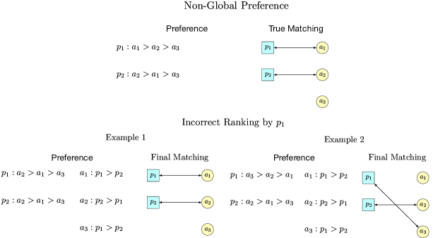
Figure 6: Examples of the matching result caused by the incorrect ranking provided by when agent $p_{2}$ submits the correct ranking list, under non-global preference. In Example 1: Agent $p_{1}$ provides the invalid ranking $p_{1}:a_{2}>a_{1}>a_{3}$. Based on the GS algorithm, the final matching result is identical to the true matching result. There is no regret created by this case. In Example 2: Agent $p_{1}$ provides the incorrect ranking $p_{1}:a_{2}>a_{3}>a_{1}$. Based on the GS algorithm, the final matching result is $(p_{1},a_{3})$ and $(p_{2},a_{2})$. It creates positive regret for $p_{1}$ and no regret for $p_{1}$. Thus, agent $p_{1}$ suffers regret and agent $p_{2}$ does not.

Appendix A5 Detailed Regret Analysis for Two Agents and Three Arms

Due to the incorrect raking from agent $p_{1}$, it creates six cases in total. In the following passage, we will analyze them case by case.

Case 1. If agent $p_{1}$ wrongly estimates the ranking over arms as $p_{1}:a_{3}>a_{1}>a_{2}$, the matching result by GS algorithm is shown in Figure 3 Case 1. Agent $p_{1}$ is matched with $a_{3}$ and agent $p_{2}$ is matched with $a_{2}$. In this case $p_{1}$ suffers a positive regret. The instantaneous regret can be decomposed as

$$R_{1,t}^{C_{1}}\overset{\Delta}{=}{\bm{\mathbf{{\theta}}}}_{1,*}^{\sf T}{\bm{\mathbf{{x}}}}_{1}(t)-{\bm{\mathbf{{\theta}}}}_{1,*}^{\sf T}{\bm{\mathbf{{x}}}}_{3}(t)={\bm{\mathbf{{\theta}}}}_{1,*}^{\sf T}({\bm{\mathbf{{x}}}}_{1}(t)-{\bm{\mathbf{{x}}}}_{3}(t)),$$ (C.24)

where we define $R_{1,t}^{C_{1}}$ is the case 1 instantaneous regret for agent $p_{1}$ at time $t$. Here $C_{1}$ represents the case 1, ”1” in the subscript represents agent $p_{1}$, and $t$ in the subscript represents the time step. Similar definitions are used in the following analysis. In addition, agent $p_{2}$ does not suffer regret in case 1.

This bad event’s joint probability for agent $p_{1}$ is the product of two ranking probabilities $\mathbb{P}_{t}^{C_{1}}\overset{\Delta}{=}\mathbb{P}_{1}\big{(}\hat{\mu}_{1,3}(t)>\hat{\mu}_{1,1}(t)>\hat{\mu}_{1,2}(t)\big{)}$ from agent $p_{1}$ and $\mathbb{P}(\mathcal{G}_{2}(t))\overset{\Delta}{=}\mathbb{P}_{2}\big{(}\hat{\mu}_{2,2}(t)>\hat{\mu}_{2,1}(t)>\hat{\mu}_{2,3}(t)\big{)}$ from agent $p_{2}$. Here we define $\mathbb{P}_{t}^{C_{1}}$ as the probability of occurring case 1 of agent $p_{1}$ and $\mathcal{G}_{2}(t)$ represents that agent $p_{2}$ submits correct ranking list to the centralized platform and we call this as the good event in the following analysis, which is equivalent to agent submitting the correct ranking list to the platform. And the bad event is equivalent to agent submitting the incorrect rankings. So this $\{\hat{\mu}_{2,2}(t)>\hat{\mu}_{2,1}(t)>\hat{\mu}_{2,3}(t)\}$ is a good event because agent $p_{2}$ correctly estimate its preference scheme over arms. $\{\hat{\mu}_{1,3}(t)>\hat{\mu}_{1,1}(t)>\hat{\mu}_{1,2}(t)\}$ is a bad event because agent $p_{1}$ wrongly estimate its preference scheme over arms. The decomposed instantaneous regret for agent $p_{1}$ is

$$\mathbb{P}(\mathcal{G}_{2}(t))\mathbb{P}_{t}^{C_{1}}R_{1,t}^{C_{1}}$$ (C.25)

$$=\mathbb{P}\big{(}\hat{\mu}_{1,3}>\hat{\mu}_{1,1}(t)>\hat{\mu}_{1,2}(t)\big{)}\mathbb{P}\big{(}\hat{\mu}_{2,2}(t)>\hat{\mu}_{2,1}(t)>\hat{\mu}_{2,3}(t)\big{)}{\bm{\mathbf{{\theta}}}}_{1,*}^{\sf T}({\bm{\mathbf{{x}}}}_{1}(t)-{\bm{\mathbf{{x}}}}_{3}(t)),$$

where the above instantaneous regret is greater than zero. For agent $p_{2}$, the decomposed instantaneous regret is

$$\mathbb{P}(\mathcal{G}_{2}(t))\mathbb{P}_{t}^{C_{1}}R_{2,t}^{C_{1}}$$ (C.26)

$$=\mathbb{P}\big{(}\hat{\mu}_{1,3}>\hat{\mu}_{1,1}(t)>\hat{\mu}_{1,2}(t)\big{)}\mathbb{P}\big{(}\hat{\mu}_{2,2}(t)>\hat{\mu}_{2,1}(t)\geq\hat{\mu}_{2,3}\big{)}{\bm{\mathbf{{\theta}}}}_{2,*}^{\sf T}({\bm{\mathbf{{x}}}}_{2}(t)-{\bm{\mathbf{{x}}}}_{2}(t))=0.$$

Case 2. If agent $p_{1}$ wrongly estimates the ranking over arms as $p_{1}:a_{3}>a_{2}>a_{1}$. The matching result by GS algorithm is in Figure 3 Case 2. Agent $p_{1}$ is matched with arm $a_{3}$ and agent $p_{2}$ is matched with arm $a_{2}$, where agent $p_{1}$ suffers a positive regret. The instantaneous regret is

$$R_{1,t}^{C_{2}}={\bm{\mathbf{{\theta}}}}_{1,*}^{\sf T}{\bm{\mathbf{{x}}}}_{1}(t)-{\bm{\mathbf{{\theta}}}}_{1,*}^{\sf T}{\bm{\mathbf{{x}}}}_{3}(t)={\bm{\mathbf{{\theta}}}}_{1,*}^{\sf T}({\bm{\mathbf{{x}}}}_{1}(t)-{\bm{\mathbf{{x}}}}_{3}(t)).$$ (C.27)

In addition, agent $p_{2}$ does not suffer regret in case 2.

This bad event’s joint probability is the product of two ranking probabilities $\mathbb{P}_{t}^{C_{2}}=\mathbb{P}\big{(}\hat{\mu}_{1,3}(t)>\hat{\mu}_{1,2}(t)>\hat{\mu}_{1,1}(t)\big{)}$ by agent $p_{1}$ and $\mathbb{P}(\mathcal{G}_{2}(t))$ by agent $p_{2}$. $\{\hat{\mu}_{1,3}(t)>\hat{\mu}_{1,2}(t)>\hat{\mu}_{1,1}(t)$ is the bad event that agent $p_{1}$ wrongly estimate its preference scheme over arms. The decomposed instantaneous regret for agent $p_{1}$ is

$$\mathbb{P}(\mathcal{G}_{2}(t))\mathbb{P}_{t}^{C_{2}}R_{1,t}^{C_{2}}$$ (C.28)

$$=\mathbb{P}\big{(}\hat{\mu}_{1,3}(t)>\hat{\mu}_{1,2}(t)>\hat{\mu}_{1,1}(t)\big{)}\mathbb{P}\big{(}\hat{\mu}_{2,2}(t)>\hat{\mu}_{2,1}(t)>\hat{\mu}_{2,3}(t)\big{)}{\bm{\mathbf{{\theta}}}}_{1,*}^{\sf T}({\bm{\mathbf{{x}}}}_{1}(t)-{\bm{\mathbf{{x}}}}_{3}(t))>0.$$

For agent $p_{2}$, the decomposed instantaneous regret is

$$\mathbb{P}(\mathcal{G}_{2}(t))\mathbb{P}_{t}^{C_{2}}R_{2,t}^{C_{2}}$$ (C.29)

$$=\mathbb{P}\big{(}\hat{\mu}_{1,3}(t)>\hat{\mu}_{1,2}(t)>\hat{\mu}_{1,1}(t)\big{)}\mathbb{P}\big{(}\hat{\mu}_{2,2}(t)>\hat{\mu}_{2,1}(t)>\hat{\mu}_{2,3}(t)\big{)}{\bm{\mathbf{{\theta}}}}_{2,*}^{\sf T}({\bm{\mathbf{{x}}}}_{2}(t)-{\bm{\mathbf{{x}}}}_{2}(t))=0.$$

This case is the same as the case 1.

Case 3. If agent $p_{1}$ wrongly estimates the ranking over arms as $p_{1}:a_{2}>a_{3}>a_{1}$. The matching result by GS algorithm is in Figure 3 Case 3. Agent $p_{1}$ is matched with arm $a_{2}$ and agent $p_{2}$ is matched with arm $a_{1}$. The decomposed instantaneous regret for agent $p_{1}$ is

$$R_{1,t}^{C_{3}}={\bm{\mathbf{{\theta}}}}_{1,*}^{\sf T}{\bm{\mathbf{{x}}}}_{1}(t)-{\bm{\mathbf{{\theta}}}}_{1,*}^{\sf T}{\bm{\mathbf{{x}}}}_{2}(t)={\bm{\mathbf{{\theta}}}}_{1,*}^{\sf T}({\bm{\mathbf{{x}}}}_{1}(t)-{\bm{\mathbf{{x}}}}_{2}(t))>0.$$ (C.30)

In addition, agent $p_{2}$ suffers a regret. The decomposed instantaneous regret for agent $p_{2}$ is

$$R_{2,t}^{C_{3}}={\bm{\mathbf{{\theta}}}}_{2,*}^{\sf T}{\bm{\mathbf{{x}}}}_{2}(t)-{\bm{\mathbf{{\theta}}}}_{2,*}^{\sf T}{\bm{\mathbf{{x}}}}_{1}(t)={\bm{\mathbf{{\theta}}}}_{2,*}^{\sf T}({\bm{\mathbf{{x}}}}_{2}(t)-{\bm{\mathbf{{x}}}}_{1}(t))>0.$$ (C.31)

This bad event’s joint probability is the product of two ranking probabilities $\mathbb{P}_{t}^{C_{3}}=\mathbb{P}\big{(}\hat{\mu}_{1,2}(t)>\hat{\mu}_{1,3}(t)>\hat{\mu}_{1,1}(t)\big{)}$ by agent $p_{1}$ and $\mathbb{P}(\mathcal{G}_{2}(t))$ by agent $p_{2}$. $\{\hat{\mu}_{1,2}(t)>\hat{\mu}_{1,3}(t)>\hat{\mu}_{1,1}(t)\}$ is the bad event that agent $p_{1}$ wrongly estimate its preference scheme over arms. The decomposed instantaneous regret for agent $p_{1}$ is

$$\mathbb{P}(\mathcal{G}_{2}(t))\mathbb{P}_{t}^{C_{3}}R_{1,t}^{C_{3}}$$ (C.32)

$$=\mathbb{P}\big{(}\hat{\mu}_{1,2}(t)>\hat{\mu}_{1,3}(t)>\hat{\mu}_{1,1}(t)\big{)}\mathbb{P}\big{(}\hat{\mu}_{2,2}(t)>\hat{\mu}_{2,1}(t)>\hat{\mu}_{2,3}(t)\big{)}{\bm{\mathbf{{\theta}}}}_{1,*}^{\sf T}({\bm{\mathbf{{x}}}}_{1}(t)-{\bm{\mathbf{{x}}}}_{2}(t))>0.$$

For agent $p_{2}$, the decomposed instantaneous regret is

$$\mathbb{P}(\mathcal{G}_{2}(t))\mathbb{P}_{t}^{C_{3}}R_{2,t}^{C_{3}}$$ (C.33)

$$=\mathbb{P}\big{(}\hat{\mu}_{1,3}(t)>\hat{\mu}_{1,1}>\hat{\mu}_{1,2}(t)\big{)}\mathbb{P}\big{(}\hat{\mu}_{2,2}(t)>\hat{\mu}_{2,1}(t)>\hat{\mu}_{2,3}(t)\big{)}{\bm{\mathbf{{\theta}}}}_{2,*}^{\sf T}({\bm{\mathbf{{x}}}}_{2}(t)-{\bm{\mathbf{{x}}}}_{1}(t))>0.$$

Case 4. If agent $p_{1}$ wrongly estimates the ranking over arms as $p_{1}:a_{2}>a_{1}>a_{3}$. The matching result by GS algorithm is in Figure 3 Case 4. Agent $p_{1}$ is matched with arm $a_{2}$ and agent $p_{2}$ is matched with arm $a_{1}$. The decomposed instantaneous regret for agent $p_{1}$ is

$$R_{1,t}^{C_{4}}={\bm{\mathbf{{\theta}}}}_{1,*}^{\sf T}{\bm{\mathbf{{x}}}}_{1}(t)-{\bm{\mathbf{{\theta}}}}_{1,*}^{\sf T}{\bm{\mathbf{{x}}}}_{2}(t)={\bm{\mathbf{{\theta}}}}_{1,*}^{\sf T}({\bm{\mathbf{{x}}}}_{1}(t)-{\bm{\mathbf{{x}}}}_{2}(t))>0.$$ (C.34)

In addition, agent $p_{2}$ suffers a positive regret. The decomposed instantaneous regret for agent $p_{2}$ is

$$R_{2,t}^{C_{4}}={\bm{\mathbf{{\theta}}}}_{2,*}^{\sf T}{\bm{\mathbf{{x}}}}_{2}(t)-{\bm{\mathbf{{\theta}}}}_{2,*}^{\sf T}{\bm{\mathbf{{x}}}}_{1}(t)={\bm{\mathbf{{\theta}}}}_{2,*}^{\sf T}({\bm{\mathbf{{x}}}}_{2}(t)-{\bm{\mathbf{{x}}}}_{1}(t))>0.$$ (C.35)

This bad event’s joint probability is the product of two ranking probabilities $\mathbb{P}_{t}^{C_{4}}=\mathbb{P}\big{(}\hat{\mu}_{1,2}(t)>\hat{\mu}_{1,1}(t)>\hat{\mu}_{1,3}(t)\big{)}$ by agent $p_{1}$ and $\mathbb{P}(\mathcal{G}_{2}(t))$ by agent $p_{2}$. $\{\hat{\mu}_{1,2}(t)>\hat{\mu}_{1,1}(t)>\hat{\mu}_{1,3}(t)\}$ is the bad event that agent $p_{1}$ wrongly estimate its preference scheme over arms. The decomposed instantaneous regret for agent $p_{1}$ is

$$\mathbb{P}(\mathcal{G}_{2}(t))\mathbb{P}_{t}^{C_{4}}R_{1,t}^{C_{4}}$$ (C.36)

$$=\mathbb{P}\big{(}\hat{\mu}_{1,2}(t)>\hat{\mu}_{1,1}(t)>\hat{\mu}_{1,3}(t)\big{)}\mathbb{P}\big{(}\hat{\mu}_{2,2}(t)>\hat{\mu}_{2,1}(t)>\hat{\mu}_{2,3}(t)\big{)}{\bm{\mathbf{{\theta}}}}_{1,*}^{\sf T}({\bm{\mathbf{{x}}}}_{1}(t)-{\bm{\mathbf{{x}}}}_{2}(t))>0.$$

For agent $p_{2}$, the decomposed instantaneous regret is

$$\mathbb{P}(\mathcal{G}_{2}(t))\mathbb{P}_{t}^{C_{4}}R_{2,t}^{C_{4}}$$ (C.37)

$$=\mathbb{P}\big{(}\hat{\mu}_{1,2}(t)>\hat{\mu}_{1,1}(t)>\hat{\mu}_{1,3}(t)\big{)}\mathbb{P}\big{(}\hat{\mu}_{2,2}(t)>\hat{\mu}_{2,1}(t)>\hat{\mu}_{2,3}(t)\big{)}{\bm{\mathbf{{\theta}}}}_{2,*}^{\sf T}({\bm{\mathbf{{x}}}}_{2}(t)-{\bm{\mathbf{{x}}}}_{1}(t))>0.$$

Case 5. If agent $p_{1}$ wrongly estimates the ranking over arms as $p_{1}:a_{1}>a_{3}>a_{2}$. The matching result by GS algorithm is in Figure 3 Case 5. Agent $p_{1}$ is matched with arm $a_{1}$ and agent $p_{2}$ is matched with arm $a_{2}$. This pair will not suffer regret. The decomposed instantaneous regret for agent $p_{1}$ is

$$R_{1,t}^{C_{5}}={\bm{\mathbf{{\theta}}}}_{1,*}^{\sf T}{\bm{\mathbf{{x}}}}_{1}(t)-{\bm{\mathbf{{\theta}}}}_{1,*}^{\sf T}{\bm{\mathbf{{x}}}}_{1}(t)={\bm{\mathbf{{\theta}}}}_{1,*}^{\sf T}({\bm{\mathbf{{x}}}}_{1}(t)-{\bm{\mathbf{{x}}}}_{1}(t))=0.$$ (C.38)

In addition, agent $p_{2}$ will not suffer a regret. The decomposed instantaneous regret for agent $p_{2}$ is

$$R_{2,t}^{C_{5}}={\bm{\mathbf{{\theta}}}}_{2,*}^{\sf T}{\bm{\mathbf{{x}}}}_{2}(t)-{\bm{\mathbf{{\theta}}}}_{2,*}^{\sf T}{\bm{\mathbf{{x}}}}_{2}(t)={\bm{\mathbf{{\theta}}}}_{2,*}^{\sf T}({\bm{\mathbf{{x}}}}_{2}(t)-{\bm{\mathbf{{x}}}}_{2}(t))=0.$$ (C.39)

This bad event’s joint probability is the product of two ranking probabilities $\mathbb{P}_{t}^{C_{5}}=\mathbb{P}\big{(}\hat{\mu}_{1,1}(t)>\hat{\mu}_{1,3}(t)>\hat{\mu}_{1,2}(t)\big{)}$ by agent $p_{1}$ and $\mathbb{P}(\mathcal{G}_{2}(t))$ by agent $p_{2}$. $\{\hat{\mu}_{1,1}(t)>\hat{\mu}_{1,3}(t)>\hat{\mu}_{1,2}(t)\}$ is the bad event that agent $p_{1}$ wrongly estimate its preference scheme over arms. The decomposed instantaneous regret for agent $p_{1}$ is

$$\mathbb{P}(\mathcal{G}_{2}(t))\mathbb{P}_{t}^{C_{5}}R_{1,t}^{C_{5}}$$ (C.40)

$$=\mathbb{P}\big{(}\hat{\mu}_{1,1}(t)>\hat{\mu}_{1,3}(t)>\hat{\mu}_{1,2}(t)\big{)}\mathbb{P}\big{(}\hat{\mu}_{2,2}(t)>\hat{\mu}_{2,1}(t)>\hat{\mu}_{2,3}(t)\big{)}{\bm{\mathbf{{\theta}}}}_{1,*}^{\sf T}({\bm{\mathbf{{x}}}}_{1}(t)-{\bm{\mathbf{{x}}}}_{1}(t))=0.$$

For agent $p_{2}$, the decomposed instantaneous regret is

$$\mathbb{P}(\mathcal{G}_{2}(t))\mathbb{P}_{t}^{C_{5}}R_{2,t}^{C_{5}}$$ (C.41)

$$=\mathbb{P}\big{(}\hat{\mu}_{1,1}(t)>\hat{\mu}_{1,3}(t)>\hat{\mu}_{1,2}(t)\big{)}\mathbb{P}\big{(}\hat{\mu}_{2,2}(t)>\hat{\mu}_{2,1}(t)>\hat{\mu}_{2,3}(t)\big{)}{\bm{\mathbf{{\theta}}}}_{2,*}^{\sf T}({\bm{\mathbf{{x}}}}_{2}(t)-{\bm{\mathbf{{x}}}}_{2}(t))=0.$$

This setting will not create any regret.

Case 6. If agent $p_{1}$ correctly estimates the ranking over arms as $p_{1}:a_{1}>a_{2}>a_{3}$. The matching result by GS algorithm is in Figure 3 Case 6. Agent $p_{1}$ is matched with arm $a_{1}$ and agent $p_{2}$ is matched with arm $a_{2}$. This pair will not suffer regret. The decomposed instantaneous regret for agent $p_{1}$ is

$$R_{1,t}^{C_{6}}={\bm{\mathbf{{\theta}}}}_{1,*}^{\sf T}{\bm{\mathbf{{x}}}}_{1}(t)-{\bm{\mathbf{{\theta}}}}_{1,*}^{\sf T}{\bm{\mathbf{{x}}}}_{1}(t)={\bm{\mathbf{{\theta}}}}_{1,*}^{\sf T}({\bm{\mathbf{{x}}}}_{1}(t)-{\bm{\mathbf{{x}}}}_{1}(t))=0.$$ (C.42)

In addition, agent $p_{2}$ will not suffer a regret. The decomposed instantaneous regret for agent $p_{1}$ is

$$R_{2,t}^{C_{6}}={\bm{\mathbf{{\theta}}}}_{2,*}^{\sf T}{\bm{\mathbf{{x}}}}_{2}(t)-{\bm{\mathbf{{\theta}}}}_{2,*}^{\sf T}{\bm{\mathbf{{x}}}}_{2}(t)={\bm{\mathbf{{\theta}}}}_{2,*}^{\sf T}({\bm{\mathbf{{x}}}}_{2}(t)-{\bm{\mathbf{{x}}}}_{2}(t))=0.$$ (C.43)

This bad event’s joint probability is the product of two ranking probabilities $\mathbb{P}_{t}^{C_{6}}=\mathbb{P}\big{(}\hat{\mu}_{1,1}(t)>\hat{\mu}_{1,2}(t)>\hat{\mu}_{1,3}(t)\big{)}$ by agent $p_{1}$, which in fact is a good event and $\mathbb{P}(\mathcal{G}_{2}(t))$ by agent $p_{2}$. $\{\hat{\mu}_{1,1}(t)>\hat{\mu}_{1,2}(t)>\hat{\mu}_{1,3}(t)\}$ is the good event that agent $p_{1}$ correctly estimate its preference scheme over arms. The decomposed instantaneous regret for agent $p_{1}$ is

$$\mathbb{P}(\mathcal{G}_{2}(t))\mathbb{P}_{t}^{C_{6}}R_{1,t}^{C_{6}}$$ (C.44)

$$=\mathbb{P}\big{(}\hat{\mu}_{1,1}(t)>\hat{\mu}_{1,2}(t)>\hat{\mu}_{1,3}(t)\big{)}\mathbb{P}\big{(}\hat{\mu}_{2,2}(t)>\hat{\mu}_{2,1}(t)>\hat{\mu}_{2,3}(t)\big{)}{\bm{\mathbf{{\theta}}}}_{1,*}^{\sf T}({\bm{\mathbf{{x}}}}_{1}(t)-{\bm{\mathbf{{x}}}}_{1}(t))=0,$$

For agent $p_{2}$, the decomposed instantaneous regret is

$$\mathbb{P}(\mathcal{G}_{2}(t))\mathbb{P}_{t}^{C_{6}}R_{2,t}^{C_{6}}$$ (C.45)

$$=\mathbb{P}\big{(}\hat{\mu}_{1,1}(t)>\hat{\mu}_{1,3}(t)>\hat{\mu}_{1,2}(t)\big{)}\mathbb{P}\big{(}\hat{\mu}_{2,2}(t)>\hat{\mu}_{2,1}(t)>\hat{\mu}_{2,3}(t)\big{)}{\bm{\mathbf{{\theta}}}}_{2,*}^{\sf T}({\bm{\mathbf{{x}}}}_{2}(t)-{\bm{\mathbf{{x}}}}_{2}(t))=0.$$

This setting will also not create any regret.

In summary, for agent $p_{1}$, the four regret occurred cases are represented in Case 1 to Case 4, two regret vanished cases happen at Case 5 and Case 6. For agent $p_{2}$, the two regret occurred cases are represented in Case 3 and Case 4, four regret vanishing cases happen at Case 1, Case 2, Case 5, and Case 6. These six cases represent all the possible regret occurring cases when $p_{1}$ submits incorrect ranking and $p_{2}$ submits correct ranking.

Appendix A6 Definitions and Lemmas of Probability Lower Bounds

In this section, we quantify the probability lower bound of the above six cases (good events and bad events) and the correct ranking $\mathcal{G}_{2}(t)$’s probability lower bound proposed by agent $p_{2}$ at time $t$.

First, without loss of generality, suppose that the true preference from the specific agent $p_{i}$ to all three arms is $a_{j_{1}}<_{i}^{t}a_{j_{2}}<_{i}^{t}a_{j_{3}}$ at time $t$, where $\{j_{1},j_{2},j_{3}\}$ is a specific permutation of $[3]=\{1,2,3\}$. This facilitates analyzing these six cases as a whole. In the following, we analyze the specific agent $p_{i}$’s instance-dependent lower bound with the preference $a_{j_{1}}<_{i}^{t}a_{j_{2}}<_{i}^{t}a_{j_{3}}$ at time $t$.

The exploitation stage’s regret is the expected regret caused by the existing bad events, which causes agents to suffer regret. The detailed definition of the bad and good events is shown as follows.

Definition 2

For agent $p_{i}$, if the true preference from agent $p_{i}$ to arms is $a_{j_{1}}<_{i}^{t}a_{j_{2}}<_{i}^{t}a_{j_{3}}$ at time $t$, where $\{j_{1},j_{2},j_{3}\}$ is a permutation of $[3]$, the good event (correct ranking) for agent $p_{i}$ is $\mathcal{G}_{i}(t)=\{\hat{\mu}_{i,j_{1}}(t)>\hat{\mu}_{i,j_{2}}(t)>\hat{\mu}_{i,j_{3}}(t)\}$. Consequently, the bad event (incorrect ranking) for agent $p_{i}$ is the complementary event of the good event, $\mathcal{G}_{i}^{c}(t)=\{\hat{\mu}_{i,j_{1}}(t)>\hat{\mu}_{i,j_{2}}(t)>\hat{\mu}_{i,j_{3}}(t)\}^{c}$.

If $(j_{1},j_{2},j_{3})=(1,2,3)$ and $i=1$, it matches agent $p_{1}$’s true preference in Figure 2.

If there exists equal estimated mean rewards, arms will be arbitrarily placed. In order to derive the instance-dependent lower bound, we have to quantify the lower bound of the good event’s probability in Lemma 5 and the lower bound of bad event’s probability in Lemma 6.

Lemma 5

If the true preference for agent $p_{i}$ over all arms is $a_{j_{1}}<_{i}^{t}a_{j_{2}}<_{i}^{t}a_{j_{3}}$ at time step $t$ and $\{j_{1},j_{2},j_{3}\}$ is a permutation $[3]$, the probability of the good event $\mathcal{G}_{i}(t)$ is lower bounded by

$$\mathbb{P}(\mathcal{G}_{i}(t)) \geq 1-\frac{1}{\nu_{i,(j_{1},j_{2})}(t)}\frac{1}{\sqrt{2\pi}}e^{(-\frac{\nu^{2}_{i,(j_{1},j_{2})}(t)}{2})}$$ (C.46)

$$-\frac{1}{\nu_{i,(j_{1},j_{3})}(t)}\frac{1}{\sqrt{2\pi}}e^{(-\frac{\nu^{2}_{i,(j_{1},j_{3})}(t)}{2})}-\frac{1}{\nu_{i,(j_{2},j_{3})}(t)}\frac{1}{\sqrt{2\pi}}e^{(-\frac{\nu^{2}_{i,(j_{2},j_{3})}(t)}{2})},$$

where $\nu_{i,(j_{1},j_{2})}(t)$ represents the scaled mean difference of the arm $a_{1}$ and the arm $a_{2}$ from the perspective of $\bar{{\bm{\mathbf{{\theta}}}}}_{i}$ at time $t$ and $\nu_{i,(j_{1},j_{3})}(t)$ and $\nu_{i,(j_{2},j_{3})}(t)$ are defined similarly in the end of supplementary material.

Lemma 6

If the true preference for agent $p_{i}$ over all arms is $a_{j_{1}}<_{i}^{t}a_{j_{2}}<_{i}^{t}a_{j_{3}}$ at time step $t$ and $\{j_{1},j_{2},j_{3}\}$ is a permutation $[3]$, the probability of the bad events satisfies,

$$\mathbb{P}\big{(}\mathcal{G}_{i}^{c}(t)\big{)} \geq\min\Big{\{}(\frac{1}{\tilde{\nu}_{i,(j_{1},j_{2})}(t)}-\frac{1}{\tilde{\nu}^{3}_{i,(j_{1},j_{2})}(t)})e^{(-\frac{\tilde{\nu}^{2}_{i,(j_{1},j_{2})}(t)}{2})},$$ (C.47)

$$\quad\quad\quad(\frac{1}{\tilde{\nu}_{i,(j_{2},j_{3})}(t)}-\frac{1}{\tilde{\nu}^{3}_{i,(j_{2},j_{3})}(t)})e^{(-\frac{\tilde{\nu}^{2}_{i,(j_{2},j_{3})}(t)}{2})}\Big{\}}$$

where $\tilde{\nu}_{i,(j_{1},j_{2})}(t),\tilde{\nu}_{i,(j_{2},j_{3})}(t)$ are the scaled mean difference defined in supplementary material.

Lemma 5 and Lemma 6 are used to getting the good event’s and bad event’s lower bounds via the sharp Gaussian tail probability lower bound at each time step in the exploitation stage, which facilitates the calculation of instantaneous regret at each time step.

Lemma 7

With Lemma 5 and Lemma 6, for time step $t>\overline{h}$, under the design of problem instance in Section 5.1, the probabilities of the good event and the bad event satisfy,

$$\mathbb{P}(\mathcal{G}_{i}(t))\geq\mathcal{L}_{i}^{g}(t),\quad\mathbb{P}\big{(}\mathcal{G}_{i}^{c}(t)\big{)}\geq\mathcal{L}_{i}^{b}(t),$$ (C.48)

where $\mathcal{L}_{i}^{g}(t)=1-\frac{3}{\sqrt{2\pi}}\frac{1}{c_{5}(t)\sqrt{\overline{h}}}e^{\big{(}-\frac{c_{5}^{2}(t)}{2}\overline{h}\big{)}}$, $\mathcal{L}_{i}^{b}(t)=(\frac{1}{c_{7}(t)\sqrt{\overline{h}}}-\frac{1}{c_{7}^{3}(t)\overline{h}^{3/2}})e^{\big{(}-\frac{c_{7}^{2}(t)}{2}\overline{h}\big{)}}$, and $c_{5}(t),c_{7}(t)$ are contextual time-dependent constants but independent of designing exploration rounds $\overline{h}$. The definitions of $c_{5}(t),c_{7}(t)$ are given in supplementary material.

Lemma 7 provides the order of lower bounds of the good event and the bad event, where we ignore context time-dependent constants.

Appendix A7 Proof of Theorem 2 - Instance Dependent Lower Bound

After $\overline{h}$ rounds of exploration, for agent $p_{i}$, its estimator $\widehat{{\bm{\mathbf{{\theta}}}}}_{i}(t)$ follows the normal distribution as showed in Eq. (10). Thus at time step $t$, the estimated mean reward for arm $a_{j}$ from the viewpoint of agent $p_{i}$ is $\hat{\mu}_{i,j}(t)=\widehat{{\bm{\mathbf{{\theta}}}}}_{i}(t)^{\sf T}{\bm{\mathbf{{x}}}}_{j}(t)$, which provides the basis to construct the ranking list $\hat{{\bm{\mathbf{{r}}}}}_{i,[K]}(t)$. Besides, since all contexts are from uniform distribution, conditioning on all previous information $\mathcal{F}_{i}(\overline{h})$ and contextual information of ${\bm{\mathbf{{x}}}}_{j}(t)$, we have the distribution of the estimated mean reward $\hat{\mu}_{i,j}(t)$ following the normal distribution

$$\hat{\mu}_{i,j}(t)=\widehat{{\bm{\mathbf{{\theta}}}}}_{i}(t)^{\sf T}{\bm{\mathbf{{x}}}}_{j}(t)|\mathcal{F}_{i}(\overline{h})\sim N(\bar{{\bm{\mathbf{{\theta}}}}}_{i}^{\sf T}{\bm{\mathbf{{x}}}}_{j}(t),\sigma^{2}{\bm{\mathbf{{x}}}}_{j}(t)^{\sf T}{\bm{\mathbf{{M}}}}_{i}{\bm{\mathbf{{x}}}}_{j}(t)),\quad\forall j\in\mathcal{K},$$ (C.49)

where $\mathbb{E}[\widehat{{\bm{\mathbf{{\theta}}}}}_{i}(t)|\mathcal{F}_{i}(\overline{h})]=\bar{{\bm{\mathbf{{\theta}}}}}_{i}=\big{(}{\bm{\mathbf{{X}}}}_{i}(\overline{h})^{\sf T}{\bm{\mathbf{{X}}}}_{i}(\overline{h})+\lambda_{i}{\bm{\mathbf{{I}}}}\big{)}^{-1}{\bm{\mathbf{{X}}}}_{i}(\overline{h})^{\sf T}{\bm{\mathbf{{X}}}}_{i}(\overline{h}){\bm{\mathbf{{\theta}}}}_{i,*}\in\mathbb{R}^{d}$, and $\text{Cov}[\widehat{{\bm{\mathbf{{\theta}}}}}_{i}(t)|\mathcal{F}_{i}(\overline{h})]=\sigma^{2}{\bm{\mathbf{{M}}}}_{i}=\sigma^{2}\big{(}{\bm{\mathbf{{X}}}}_{i}(\overline{h})^{\sf T}{\bm{\mathbf{{X}}}}_{i}(\overline{h})+\lambda_{i}{\bm{\mathbf{{I}}}}\big{)}^{-1}{\bm{\mathbf{{X}}}}_{i}(\overline{h})^{\sf T}{\bm{\mathbf{{X}}}}_{i}(\overline{h})\big{(}{\bm{\mathbf{{X}}}}_{i}(\overline{h})^{\sf T}{\bm{\mathbf{{X}}}}_{i}(\overline{h})+\lambda_{i}{\bm{\mathbf{{I}}}}\big{)}^{-1}\in\mathbb{R}^{d\times d}$.

With the distribution of $\hat{\mu}_{i,j}(t)$, to derive the regret lower bound, we first evaluate good events $\mathcal{G}_{1}(t)$ and $\mathcal{G}_{2}(t)$’s probability lower bound in Section A7.1, and bad events $\mathcal{G}_{1}^{c}(t)$ and $\mathcal{G}_{2}^{c}(t)$’s lower bound in Section A7.2. In addition, we provide good events and bad events’ probability lower bounds’ corresponding order at time $t$, which is provided in Section A7.3. In Section A7.4, we provide the final instance-dependent regret lower bound as a whole. In Section

A7.1 Proof of Lemma 5

Proof. First, without loss of generality, suppose that the true preference from agent $p_{i}$ to all arms is $a_{j_{1}}<_{i}^{t}a_{j_{2}}<_{i}^{t}a_{j_{3}}$ at time $t$. In order to present the competing status of those agents, we need to quantify the probability of the good event $\mathcal{G}_{i}(t)=\{\hat{\mu}_{i,j_{1}}(t)>\hat{\mu}_{i,j_{2}}(t)>\hat{\mu}_{i,j_{3}}(t)\}$. Here we denote $\mathcal{A}(t)=\{\hat{\mu}_{i,j_{1}}(t)>\max(\hat{\mu}_{i,j_{2}}(t),\hat{\mu}_{i,j_{3}}(t))\}$ as the 1st-good event and $\mathcal{B}(t)=\{\hat{\mu}_{i,j_{2}}(t)>\hat{\mu}_{i,j_{3}}(t)\}$ as the 2nd-good event, where $\mathcal{G}_{i}(t)=\mathcal{A}(t)\cap\mathcal{B}(t)$. Here we omit the index ’i’ in 1st-good event and 2nd-good event. The 1st-good event $\mathcal{A}$ can also be divided into to the event $\mathcal{A}_{1}(t)=\{\hat{\mu}_{i,j_{1}}(t)>\hat{\mu}_{i,j_{2}}(t)\}$ and the event $\mathcal{A}_{2}(t)=\{\hat{\mu}_{i,j_{1}}(t)>\hat{\mu}_{i,j_{3}}(t)\}$ happening simultaneously, where $\mathcal{A}(t)=\mathcal{A}_{1}(t)\cap\mathcal{A}_{2}(t)$. By the property of $\mathbb{P}(\mathcal{A}(t)\cap\mathcal{B}(t))\geq\mathbb{P}(\mathcal{A}(t))+\mathbb{P}(\mathcal{B}(t))-\mathbb{P}(\mathcal{A}(t)\cup\mathcal{B}(t))\geq\mathbb{P}(\mathcal{A}(t))+\mathbb{P}(\mathcal{B}(t))-1$, we use the same technique again and have $\mathbb{P}(\mathcal{A}(t))\geq\mathbb{P}(\mathcal{A}_{1}(t))+\mathbb{P}(\mathcal{A}_{2}(t))-1$. So the event $\mathcal{A}(t)$’s probability lower bound is,

$$\mathbb{P}(\mathcal{A}(t)) =\mathbb{P}(\hat{\mu}_{i,j_{1}}(t)>\max(\hat{\mu}_{i,j_{2}}(t),\hat{\mu}_{i,j_{3}}(t)))$$ (C.50)

$$=\mathbb{P}(\{\hat{\mu}_{i,j_{1}}(t)>\hat{\mu}_{i,j_{2}}(t)\}\cap\{\hat{\mu}_{i,j_{1}}(t)>\hat{\mu}_{i,j_{3}}(t)\})$$

$$\geq\mathbb{P}(\hat{\mu}_{i,j_{1}}(t)>\hat{\mu}_{i,j_{2}}(t))+\mathbb{P}(\hat{\mu}_{i,j_{1}}(t)>\hat{\mu}_{i,j_{3}}(t))-1$$

$$=\mathbb{P}(\mathcal{A}_{1}(t))+\mathbb{P}(\mathcal{A}_{2}(t))-1.$$

Now we have to quantify the event $\mathcal{A}_{1}(t)$ and event $\mathcal{A}_{2}(t)$’s probabilities’ lower bound. We first define the estimated mean reward difference for agent $p_{i}$ at time $t$ between arm $a_{j_{1}}$ and arm $a_{j_{2}}$ as $\hat{Z}_{i,(j_{1},j_{2})}=\hat{\mu}_{i,j_{1}}(t)-\hat{\mu}_{i,j_{2}}(t)$. Given all contextual information at time $t$, we get

$$\hat{Z}_{i,(j_{1},j_{2})}|\mathcal{F}_{i}(\overline{h})\sim N(\bar{{\bm{\mathbf{{\theta}}}}}_{i}^{\sf T}[{\bm{\mathbf{{x}}}}_{j_{1}}(t)-{\bm{\mathbf{{x}}}}_{j_{2}}(t)],\tilde{\Sigma}_{i,(j_{1},j_{2})}(t)),$$ (C.51)

where $\tilde{\Sigma}_{i,(j_{1},j_{2})}(t)=\sigma^{2}[{\bm{\mathbf{{x}}}}_{j_{1}}(t)^{\sf T}{\bm{\mathbf{{M}}}}_{i}{\bm{\mathbf{{x}}}}_{j_{1}}(t)+{\bm{\mathbf{{x}}}}_{j_{2}}(t)^{\sf T}{\bm{\mathbf{{M}}}}_{i}{\bm{\mathbf{{x}}}}_{j_{2}}(t)-2{\bm{\mathbf{{x}}}}_{j_{1}}(t)^{\sf T}{\bm{\mathbf{{M}}}}_{i}{\bm{\mathbf{{x}}}}_{j_{2}}(t)]\in\mathbb{R}$ is the variance of the estimated mean reward $\hat{\mu}_{i,j_{1}}(t)-\hat{\mu}_{i,j_{2}}(t)$. We know that $\hat{\mu}_{i,j_{1}}(t)$ and $\hat{\mu}_{i,j_{2}}(t)$ are positively correlated because ${\bm{\mathbf{{M}}}}_{i}$ is positive semi-definite since ${\bm{\mathbf{{x}}}}_{j_{1}}$ and ${\bm{\mathbf{{x}}}}_{j_{2}}$’s coordinates are follow uniform distribution $U(0,1)^{d}$. So the variance of the difference $\hat{\mu}_{i,j_{1}}(t)-\hat{\mu}_{i,j_{2}}(t)$ of the two correlated normal random variables is less than the variance of the difference of two independent normal random variables by the property $var(\varpi_{1}-\varpi_{2})\leq var(\varpi_{1})+var(\varpi_{2})$ if $\varpi_{1}$ and $\varpi_{2}$ are positively correlated random variables. Besides, we know if two normal random variables $\hat{\mu}_{i,j_{1}}(t)$ and $\hat{\mu}_{i,j_{2}}(t)$ are independent,

$$\tilde{\Sigma}_{i,(j_{1},j_{2})}(t)\leq\sigma^{2}[{\bm{\mathbf{{x}}}}_{j_{1}}(t)^{\sf T}{\bm{\mathbf{{M}}}}_{i}{\bm{\mathbf{{x}}}}_{j_{1}}(t)+{\bm{\mathbf{{x}}}}_{j_{2}}(t)^{\sf T}{\bm{\mathbf{{M}}}}_{i}{\bm{\mathbf{{x}}}}_{j_{2}}(t)],$$ (C.52)

where ${\bm{\mathbf{{x}}}}_{j_{1}}(t)^{\sf T}{\bm{\mathbf{{M}}}}_{i}{\bm{\mathbf{{x}}}}_{j_{1}}(t)$ and ${\bm{\mathbf{{x}}}}_{j_{2}}(t)^{\sf T}{\bm{\mathbf{{M}}}}_{i}{\bm{\mathbf{{x}}}}_{j_{2}}(t)$ are the variances of $\hat{\mu}_{i,j_{1}}(t)$ and $\hat{\mu}_{i,j_{2}}(t)$ correspondingly, and we define $\Sigma_{i,(j_{1},j_{2})}(t)=\sigma^{2}[{\bm{\mathbf{{x}}}}_{j_{1}}(t)^{\sf T}{\bm{\mathbf{{M}}}}_{i}{\bm{\mathbf{{x}}}}_{j_{1}}(t)+{\bm{\mathbf{{x}}}}_{j_{2}}(t)^{\sf T}{\bm{\mathbf{{M}}}}_{i}{\bm{\mathbf{{x}}}}_{j_{2}}(t)]$. We use the proxy random variable $Z_{i,(j_{1},j_{2})}$ to define the difference of two independent Gaussian random variables. $Z_{i,(j_{1},j_{2})}$’s distribution follows the normal distribution

$$Z_{i,(j_{1},j_{2})}|\mathcal{F}_{i}(\overline{h})\sim N(\bar{{\bm{\mathbf{{\theta}}}}}_{i}^{\sf T}[{\bm{\mathbf{{x}}}}_{j_{1}}(t)-{\bm{\mathbf{{x}}}}_{j_{2}}(t)],\Sigma_{i,(j_{1},j_{2})}(t)),$$ (C.53)

where $\bar{{\bm{\mathbf{{\theta}}}}}_{i}^{\sf T}[{\bm{\mathbf{{x}}}}_{j_{1}}(t)-{\bm{\mathbf{{x}}}}_{j_{2}}(t)]$ is the $Z_{i,(j_{1},j_{2})}$’s expectation and $\Sigma_{i,(j_{1},j_{2})}(t)$ is the variance of $Z_{i,(j_{1},j_{2})}$. In the following passage, we omit the filtration $|\mathcal{F}_{i}(\overline{h})$ in argument. Then we can obtain the probability lower bound of arm $a_{j_{1}}$ is ranked higher than the arm $a_{j_{2}}$ at time step $t$ from the viewpoint of agent $p_{i}$ via the proxy random variable $Z_{i,(j_{1},j_{2})}$, that is

$$\mathbb{P}(\hat{\mu}_{i,j_{1}}(t)>\hat{\mu}_{i,j_{2}}(t)) =\mathbb{P}(\hat{\mu}_{i,j_{1}}(t)-\hat{\mu}_{i,j_{2}}(t)>0)$$ (C.54)

$$=\mathbb{P}(\hat{Z}_{i,(j_{1},j_{2})}>0)$$

$$\geq\mathbb{P}(Z_{i,(j_{1},j_{2})}>0),\;\text{by the inequality }\eqref{Eq: normal variance comparison}$$

$$=\mathbb{P}\Bigg{(}\frac{Z_{i,(j_{1},j_{2})}-\bar{{\bm{\mathbf{{\theta}}}}}_{i}^{\sf T}[{\bm{\mathbf{{x}}}}_{j_{1}}(t)-{\bm{\mathbf{{x}}}}_{j_{2}}(t)]}{\Sigma_{i,(j_{1},j_{2})}(t)}\geq-\nu_{i,(j_{1},j_{2})}(t)\Bigg{)},$$

where $\nu_{i,(j_{1},j_{2})}(t)=\frac{\bar{{\bm{\mathbf{{\theta}}}}}_{i}^{\sf T}[{\bm{\mathbf{{x}}}}_{j_{1}}(t)-{\bm{\mathbf{{x}}}}_{j_{2}}(t)]}{\Sigma_{i,(j_{1},j_{2})}(t)}$ greater than zero, is based on the true preference’s setting that $a_{j_{1}}>_{i}^{t}a_{j_{2}}>_{i}^{t}a_{j_{3}}$ for agent $p_{i}$ at time $t$. The aim of the last equality is to transform the proxy random variable to the standard normal variable and quantify the event $\mathcal{A}_{1}(t)$’s probability lower bound. Now this event $\mathcal{A}_{1}(t)$’s probability lower bound is

$$\mathbb{P}(\hat{\mu}_{i,j_{1}}(t)>\hat{\mu}_{i,j_{2}}(t)) \geq 1-\mathbb{P}\Bigg{(}\frac{Z_{i,(j_{1},j_{2})}-\bar{{\bm{\mathbf{{\theta}}}}}_{i}^{\sf T}[{\bm{\mathbf{{x}}}}_{j_{1}}(t)-{\bm{\mathbf{{x}}}}_{j_{2}}(t)]}{\Sigma_{i,(j_{1},j_{2})}(t)}\geq\nu_{i,(j_{1},j_{2})}(t)\Bigg{)}$$ (C.55)

$$\geq 1-\frac{1}{\nu_{i,(j_{1},j_{2})}(t)}\frac{1}{\sqrt{2\pi}}e^{\bigg{(}-\frac{\nu^{2}_{i,(j_{1},j_{2})}(t)}{2}\bigg{)}},$$

where the last inequality is by Lemma 2, which provides the tail probability of the normal distribution since $\nu_{i,(j_{1},j_{2})}(t)$ is positive. With the same technique, we can acquire the event $\mathcal{A}_{2}(t)$’s probability’s lower bound and we also define $\nu_{t,(j_{1},j_{3})}=\frac{\bar{{\bm{\mathbf{{\theta}}}}}_{i}^{\sf T}[{\bm{\mathbf{{x}}}}_{j_{1}}(t)-{\bm{\mathbf{{x}}}}_{j_{3}}(t)]}{\Sigma_{i,(j_{1},j_{3})}(t)}$, which is greater than zero. Then we have

$$\mathbb{P}(\hat{\mu}_{i,j_{1}}(t)>\hat{\mu}_{i,j_{3}}(t))\geq 1-\frac{1}{\nu_{t,(j_{1},j_{3})}}\frac{1}{\sqrt{2\pi}}e^{\bigg{(}-\frac{\nu_{t,(j_{1},j_{3})}^{2}}{2}\bigg{)}}.$$ (C.56)

So the 1st-good event’s lower bound probability is,

$$\mathbb{P}(\hat{\mu}_{i,j_{1}}(t)>\max(\hat{\mu}_{i,j_{2}}(t),\hat{\mu}_{i,j_{3}}(t)))$$ (C.57)

$$\geq 1-\frac{1}{\nu_{i,(j_{1},j_{2})}(t)}\frac{1}{\sqrt{2\pi}}e^{\bigg{(}-\frac{\nu^{2}_{i,(j_{1},j_{2})}(t)}{2}\bigg{)}}+1-\frac{1}{\nu_{t,(j_{1},j_{3})}}\frac{1}{\sqrt{2\pi}}e^{\bigg{(}-\frac{\nu_{t,(j_{1},j_{3})}^{2}}{2}\bigg{)}}-1$$

$$=1-\frac{1}{\nu_{i,(j_{1},j_{2})}(t)}\frac{1}{\sqrt{2\pi}}e^{\bigg{(}-\frac{\nu^{2}_{i,(j_{1},j_{2})}(t)}{2}\bigg{)}}-\frac{1}{\nu_{t,(j_{1},j_{3})}}\frac{1}{\sqrt{2\pi}}e^{\bigg{(}-\frac{\nu_{t,(j_{1},j_{3})}^{2}}{2}\bigg{)}}.$$

And the 2nd-good event’s lower bound probability is,

$$\mathbb{P}(\hat{\mu}_{i,j_{2}}(t)>\hat{\mu}_{i,j_{3}}(t))\geq 1-\frac{1}{\nu_{i,(j_{2},j_{3})}(t)}\frac{1}{\sqrt{2\pi}}e^{\bigg{(}-\frac{\nu^{2}_{i,(j_{2},j_{3})}(t)}{2}\bigg{)}},$$ (C.58)

where $\nu_{t,(j_{2},j_{3})}=\frac{\bar{{\bm{\mathbf{{\theta}}}}}_{i}^{\sf T}[{\bm{\mathbf{{x}}}}_{j_{2}}(t)-{\bm{\mathbf{{x}}}}_{j_{3}}(t)]}{\Sigma_{i,(j_{2},j_{3})}(t)}>0$ and we define $\Sigma_{i,(j_{2},j_{3})}(t)=\sigma^{2}[{\bm{\mathbf{{x}}}}_{j_{2}}(t)^{\sf T}{\bm{\mathbf{{M}}}}_{i}{\bm{\mathbf{{x}}}}_{j_{2}}(t)+{\bm{\mathbf{{x}}}}_{j_{3}}(t)^{\sf T}{\bm{\mathbf{{M}}}}_{i}{\bm{\mathbf{{x}}}}_{j_{3}}(t)]$.

Here we provide all definitions of $\Sigma_{i,(j_{1},j_{2})}(t)$, $\Sigma_{i,(j_{2},j_{3})}(t)$, and $\Sigma_{i,(j_{1},j_{3})}(t)$,

$$\nu_{i,(j_{1},j_{2})}(t)=\frac{\bar{{\bm{\mathbf{{\theta}}}}}_{i}^{\sf T}[{\bm{\mathbf{{x}}}}_{j_{1}}(t)-{\bm{\mathbf{{x}}}}_{j_{2}}(t)]}{\Sigma_{i,(j_{1},j_{2})}(t)},\Sigma_{i,(j_{1},j_{2})}(t)=\sigma^{2}[{\bm{\mathbf{{x}}}}_{j_{1}}(t)^{\sf T}{\bm{\mathbf{{M}}}}_{i}{\bm{\mathbf{{x}}}}_{j_{1}}(t)+{\bm{\mathbf{{x}}}}_{j_{2}}(t)^{\sf T}{\bm{\mathbf{{M}}}}_{i}{\bm{\mathbf{{x}}}}_{j_{2}}(t)]$$ (C.59)

$$\nu_{i,(j_{2},j_{3})}(t)=\frac{\bar{{\bm{\mathbf{{\theta}}}}}_{i}^{\sf T}[{\bm{\mathbf{{x}}}}_{j_{2}}(t)-{\bm{\mathbf{{x}}}}_{j_{3}}(t)]}{\Sigma_{i,(j_{2},j_{3})}(t)},\Sigma_{i,(j_{2},j_{3})}(t)=\sigma^{2}[{\bm{\mathbf{{x}}}}_{j_{2}}(t)^{\sf T}{\bm{\mathbf{{M}}}}_{i}{\bm{\mathbf{{x}}}}_{j_{2}}(t)+{\bm{\mathbf{{x}}}}_{j_{3}}(t)^{\sf T}{\bm{\mathbf{{M}}}}_{i}{\bm{\mathbf{{x}}}}_{j_{3}}(t)]$$

$$\nu_{i,(j_{1},j_{3})}(t)=\frac{\bar{{\bm{\mathbf{{\theta}}}}}_{i}^{\sf T}[{\bm{\mathbf{{x}}}}_{j_{1}}(t)-{\bm{\mathbf{{x}}}}_{j_{3}}(t)]}{\Sigma_{i,(j_{1},j_{3})}(t)},\Sigma_{i,(j_{1},j_{3})}(t)=\sigma^{2}[{\bm{\mathbf{{x}}}}_{j_{1}}(t)^{\sf T}{\bm{\mathbf{{M}}}}_{i}{\bm{\mathbf{{x}}}}_{j_{1}}(t)+{\bm{\mathbf{{x}}}}_{j_{3}}(t)^{\sf T}{\bm{\mathbf{{M}}}}_{i}{\bm{\mathbf{{x}}}}_{j_{3}}(t)]$$

So the final good event $\mathcal{G}_{i}(t)$’s probability lower bound is

$$\mathbb{P}(\mathcal{G}_{i}(t)) \geq 1-\frac{1}{\nu_{i,(j_{1},j_{2})}(t)}\frac{1}{\sqrt{2\pi}}e^{(-\frac{\nu^{2}_{i,(j_{1},j_{2})}(t)}{2})}$$ (C.60)

$$\qquad-\frac{1}{\nu_{i,(j_{1},j_{3})}(t)}\frac{1}{\sqrt{2\pi}}e^{(-\frac{\nu^{2}_{i,(j_{1},j_{3})}(t)}{2})}-\frac{1}{\nu_{i,(j_{2},j_{3})}(t)}\frac{1}{\sqrt{2\pi}}e^{(-\frac{\nu^{2}_{i,(j_{2},j_{3})}(t)}{2})}.$$

A7.2 Proof of Lemma 6

Proof. To get the probability lower bound of the bad event $\mathcal{G}_{i}^{c}(t)$, we can obtain the upper bound of the good event $\mathcal{G}_{i}(t)$ probability first. The proof path is similar to the proof of Lemma 5 but with the upper bound of the tail probability of the normal distribution and exists some nuances. We have

$$\mathbb{P}\big{(}\mathcal{G}_{i}(t)\big{)}$$ (C.61)

$$=\mathbb{P}\big{(}\hat{\mu}_{i,j_{1}}(t)-\hat{\mu}_{i,j_{2}}(t)>0,\hat{\mu}_{i,j_{2}}(t)-\hat{\mu}_{i,j_{3}}(t)>0\big{)}$$

$$=\mathbb{P}\big{(}\hat{\mu}_{i,j_{1}}(t)-\hat{\mu}_{i,j_{2}}(t)>0|\hat{\mu}_{i,j_{2}}(t)-\hat{\mu}_{i,j_{3}}(t)>0\big{)}\mathbb{P}\big{(}\hat{\mu}_{i,j_{2}}(t)-\hat{\mu}_{i,j_{3}}(t)>0\big{)}$$

$$\leq\mathbb{P}\big{(}\hat{\mu}_{i,j_{2}}(t)-\hat{\mu}_{i,j_{3}}(t)>0\big{)},$$

where the last inequality holds because $\mathbb{P}\big{(}\hat{\mu}_{i,j_{1}}(t)-\hat{\mu}_{i,j_{2}}(t)>0|\hat{\mu}_{i,j_{2}}(t)-\hat{\mu}_{i,j_{3}}(t)>0\big{)}\leq 1$. Similarly we have

$$\mathbb{P}\big{(}\mathcal{G}_{i}(t)\big{)}$$ (C.62)

$$=\mathbb{P}\big{(}\hat{\mu}_{i,j_{2}}(t)-\hat{\mu}_{i,j_{3}}(t)>0|\hat{\mu}_{i,j_{1}}(t)-\hat{\mu}_{i,j_{2}}(t)>0\big{)}\mathbb{P}\big{(}\hat{\mu}_{i,j_{1}}(t)-\hat{\mu}_{i,j_{2}}(t)>0\big{)}$$

$$\leq\mathbb{P}\big{(}\hat{\mu}_{i,j_{1}}(t)-\hat{\mu}_{i,j_{2}}(t)>0\big{)},$$

where the last inequality holds because $\mathbb{P}\big{(}\hat{\mu}_{i,j_{2}}(t)-\hat{\mu}_{i,j_{3}}(t)>0|\hat{\mu}_{i,j_{1}}(t)-\hat{\mu}_{i,j_{2}}(t)>0\big{)}\leq 1$.

To get the upper bound of $\mathbb{P}\big{(}\mathcal{G}_{i}(t)\big{)}$, we need to quantify the maximum value of $\mathbb{P}\big{(}\hat{\mu}_{i,j_{1}}(t)-\hat{\mu}_{i,j_{2}}(t)>0\big{)}$ and $\mathbb{P}\big{(}\hat{\mu}_{i,j_{2}}(t)-\hat{\mu}_{i,j_{3}}(t)>0\big{)}$. Here we use the same definition in Lemma 5, $\mathcal{A}_{1}(t)=\{\hat{\mu}_{i,j_{1}}(t)>\hat{\mu}_{i,j_{2}}(t)\}$ and $\mathcal{B}(t)=\hat{\mu}_{i,j_{2}}(t)>\hat{\mu}_{i,j_{3}}(t)$. In the following, we provide the proof of getting upper bound probability of $\mathcal{B}(t)$ and $\mathcal{A}_{1}(t)$. The proof of getting the probability upper bound of two quantities is similar, so we get the upper bound of $\mathbb{P}\big{(}\mathcal{B}(t)\big{)}$ first.

Let’s use the similar notation defined in Lemma 5.

$$\hat{Z}_{i,(j_{2},j_{3})}=\hat{\mu}_{i,j_{2}}(t)-\hat{\mu}_{i,j_{3}}(t)|\mathcal{F}_{i}(\overline{h})\sim N(\bar{{\bm{\mathbf{{\theta}}}}}_{i}^{\sf T}[{\bm{\mathbf{{x}}}}_{j_{2}}(t)-{\bm{\mathbf{{x}}}}_{j_{3}}(t)],\tilde{\Sigma}_{i,(j_{2},j_{3})}),$$ (C.63)

where $\tilde{\Sigma}_{i,(j_{2},j_{3})}=\sigma^{2}[{\bm{\mathbf{{x}}}}_{j_{2}}(t)^{\sf T}{\bm{\mathbf{{M}}}}_{i}{\bm{\mathbf{{x}}}}_{j_{2}}(t)+{\bm{\mathbf{{x}}}}_{j_{3}}(t)^{\sf T}{\bm{\mathbf{{M}}}}_{i}{\bm{\mathbf{{x}}}}_{j_{3}}(t)-2{\bm{\mathbf{{x}}}}_{j_{2}}(t)^{\sf T}{\bm{\mathbf{{M}}}}_{i}{\bm{\mathbf{{x}}}}_{j_{3}}(t)]$, greater than zero, is the true variance of $\hat{Z}_{i,(j_{2},j_{3})}$. So

$$\mathbb{P}\big{(}\mathcal{B}(t)\big{)} =\mathbb{P}\big{(}\hat{Z}_{i,(j_{2},j_{3})}>0\big{)}$$ (C.64)

$$=\mathbb{P}\big{(}\frac{\hat{Z}_{i,(j_{2},j_{3})}-\bar{{\bm{\mathbf{{\theta}}}}}_{i}^{\sf T}[{\bm{\mathbf{{x}}}}_{j_{2}}(t)-{\bm{\mathbf{{x}}}}_{j_{3}}(t)]}{\tilde{\Sigma}_{i,(j_{2},j_{3})}}\geq-\tilde{\nu}_{i,(j_{2},j_{3})}(t)\big{)}$$

$$=1-\mathbb{P}\big{(}\frac{\hat{Z}_{i,(j_{2},j_{3})}-\bar{{\bm{\mathbf{{\theta}}}}}_{i}^{\sf T}[{\bm{\mathbf{{x}}}}_{j_{2}}(t)-{\bm{\mathbf{{x}}}}_{j_{3}}(t)]}{\tilde{\Sigma}_{i,(j_{2},j_{3})}}\geq\tilde{\nu}_{i,(j_{2},j_{3})}(t)\big{)}$$

where the last equality holds by the symmetry property of normal distribution and define $\tilde{\nu}_{i,(j_{2},j_{3})}(t)=\frac{\bar{{\bm{\mathbf{{\theta}}}}}_{i}^{\sf T}[{\bm{\mathbf{{x}}}}_{j_{2}}(t)-{\bm{\mathbf{{x}}}}_{j_{3}}(t)]}{\tilde{\Sigma}_{i,(j_{2},j_{3})}}$, greater than zero. Besides, $\tilde{\nu}_{i,(j_{1},j_{2})}(t)$ can be defined similarly,

$$\tilde{\nu}_{i,(j_{1},j_{2})}(t)=\frac{\bar{{\bm{\mathbf{{\theta}}}}}_{i}^{\sf T}[{\bm{\mathbf{{x}}}}_{j_{1}}(t)-{\bm{\mathbf{{x}}}}_{j_{2}}(t)]}{\tilde{\Sigma}_{i,(j_{1},j_{2})}(t)},$$ (C.65)

$$\tilde{\Sigma}_{i,(j_{1},j_{2})}(t)=\sigma^{2}[{\bm{\mathbf{{x}}}}_{j_{1}}(t)^{\sf T}{\bm{\mathbf{{M}}}}_{i}{\bm{\mathbf{{x}}}}_{j_{1}}(t)+{\bm{\mathbf{{x}}}}_{j_{2}}(t)^{\sf T}{\bm{\mathbf{{M}}}}_{i}{\bm{\mathbf{{x}}}}_{j_{2}}(t)-2{\bm{\mathbf{{x}}}}_{j_{1}}(t)^{\sf T}{\bm{\mathbf{{M}}}}_{i}{\bm{\mathbf{{x}}}}_{j_{2}}(t)].$$

So by the Lemma 2’s lower bound of normal tail probability, we have the upper bound probability of $\mathcal{B}(t)$,

$$\mathbb{P}\big{(}\mathcal{B}(t)\big{)}\leq 1-(\frac{1}{\tilde{\nu}_{i,(j_{2},j_{3})}(t)}-\frac{1}{\tilde{\nu}^{3}_{i,(j_{2},j_{3})}(t)})e^{\bigg{(}-\frac{\tilde{\nu}^{2}_{i,(j_{2},j_{3})}(t)}{2}\bigg{)}}.$$ (C.66)

So the similar result can be obtained for $\mathcal{A}_{1}(t)$,

$$\mathbb{P}\big{(}\mathcal{A}_{1}(t)\big{)}\leq 1-(\frac{1}{\tilde{\nu}_{i,(j_{1},j_{2})}(t)}-\frac{1}{\tilde{\nu}^{3}_{i,(j_{1},j_{2})}(t)})e^{\bigg{(}-\frac{\tilde{\nu}^{2}_{i,(j_{1},j_{2})}(t)}{2}\bigg{)}}.$$ (C.67)

Since

$$\mathbb{P}\big{(}\mathcal{G}_{i}(t)\big{)} \leq\max\Big{\{}\mathbb{P}\big{(}\hat{\mu}_{i,j_{2}}(t)-\hat{\mu}_{i,j_{3}}(t)>0\big{)},\mathbb{P}\big{(}\hat{\mu}_{i,j_{1}}(t)-\hat{\mu}_{i,j_{2}}(t)>0\big{)}\Big{\}},$$ (C.68)

$$\leq 1-\min\Big{\{}(\frac{1}{\tilde{\nu}_{i,(j_{2},j_{3})}(t)}-\frac{1}{\tilde{\nu}^{3}_{i,(j_{2},j_{3})}(t)})e^{\bigg{(}-\frac{\tilde{\nu}^{2}_{i,(j_{2},j_{3})}(t)}{2}\bigg{)}},$$

$$\quad\quad\quad\quad\quad(\frac{1}{\tilde{\nu}_{i,(j_{1},j_{2})}(t)}-\frac{1}{\tilde{\nu}^{3}_{i,(j_{1},j_{2})}(t)})e^{\bigg{(}-\frac{\tilde{\nu}^{2}_{i,(j_{1},j_{2})}(t)}{2}\bigg{)}}\Big{\}}.$$

Meanwhile we get the lower bound of $\mathcal{G}_{i}^{c}(t)$ as follows,

$$\mathbb{P}\big{(}\mathcal{G}_{i}^{c}(t)\big{)} \geq\min\Big{\{}(\frac{1}{\tilde{\nu}_{i,(j_{2},j_{3})}(t)}-\frac{1}{\tilde{\nu}^{3}_{i,(j_{2},j_{3})}(t)})e^{\bigg{(}-\frac{\tilde{\nu}^{2}_{i,(j_{2},j_{3})}(t)}{2}\bigg{)}},$$ (C.69)

$$\quad\quad\quad(\frac{1}{\tilde{\nu}_{i,(j_{1},j_{2})}(t)}-\frac{1}{\tilde{\nu}^{3}_{i,(j_{1},j_{2})}(t)})e^{\bigg{(}-\frac{\tilde{\nu}^{2}_{i,(j_{1},j_{2})}(t)}{2}\bigg{)}}\Big{\}}$$

A7.3 Proof of Lemma 7

Proof. In order to get the good event $\mathcal{G}_{i}(t)$ and bad event $\mathcal{G}_{i}^{c}(t)$’s probability order. We first need to analyze the order of $\nu_{i,(j_{1},j_{2})}(t)$, $\tilde{\nu}_{i,(j_{1},j_{2})}(t)$, $\Sigma_{i,(j_{2},j_{3})}(t)$, $\tilde{\Sigma}_{i,(j_{2},j_{3})}(t)$ and other similar terms.

Based on the definition of $\nu_{i,(j_{1},j_{2})}(t)=\frac{\bar{{\bm{\mathbf{{\theta}}}}}_{i}^{\sf T}[{\bm{\mathbf{{x}}}}_{j_{1}}(t)-{\bm{\mathbf{{x}}}}_{j_{2}}(t)]}{\Sigma_{i,(j_{1},j_{2})}}$, we know that the context difference at time $t$, which is ${\bm{\mathbf{{x}}}}_{j_{1}}(t)-{\bm{\mathbf{{x}}}}_{j_{2}}(t)$, independent of $\overline{h}$. The expected ridge parameter is $\bar{{\bm{\mathbf{{\theta}}}}}_{i}=\big{(}{\bm{\mathbf{{X}}}}_{i}(\overline{h})^{\sf T}{\bm{\mathbf{{X}}}}_{i}(\overline{h})+\lambda_{i}{\bm{\mathbf{{I}}}}\big{)}^{-1}{\bm{\mathbf{{X}}}}_{i}(\overline{h})^{\sf T}{\bm{\mathbf{{X}}}}_{i}(\overline{h}){\bm{\mathbf{{\theta}}}}_{i,*}$. Based on the problem design in Eq. (9), $\bar{{\bm{\mathbf{{\theta}}}}}_{i}$ can be rewritten as $\{\sqrt{1-1/\bar{h}}{\bm{\mathbf{{c}}}}_{1}+1/\sqrt{\bar{h}}{\bm{\mathbf{{c}}}}_{2}\}=1/\sqrt{\bar{h}}{\bm{\mathbf{{c}}}}_{3}$, where ${\bm{\mathbf{{c}}}}_{1},{\bm{\mathbf{{c}}}}_{2}$ are time-dependent constants based on $({\bm{\mathbf{{X}}}}_{i}(\overline{h})^{\sf T}{\bm{\mathbf{{X}}}}_{i}(\overline{h})+\lambda_{i}{\bm{\mathbf{{I}}}}\big{)}^{-1}{\bm{\mathbf{{X}}}}_{i}(\overline{h})^{\sf T}{\bm{\mathbf{{X}}}}_{i}$ but independent of $\overline{h}$, and ${\bm{\mathbf{{c}}}}_{3}$ is also a context-constant, but independent of $\overline{h}$. Besides, we know that ${\bm{\mathbf{{x}}}}_{j_{1}}(t)^{\sf T}{\bm{\mathbf{{M}}}}_{i}{\bm{\mathbf{{x}}}}_{j_{1}}(t)\leq\lambda_{\max}({\bm{\mathbf{{M}}}}_{i})||{\bm{\mathbf{{x}}}}_{j_{1}}(t)||^{2}_{2}\leq\lambda_{\max}({\bm{\mathbf{{M}}}}_{i})L$ by the property $||{\bm{\mathbf{{x}}}}_{j_{1}}(t)||^{2}_{2}\leq L$, where $L$ is a constant and we assume $L=1$. So $\lambda_{\max}({\bm{\mathbf{{M}}}}_{i})=c_{4}/\overline{h}$ by Chapter 4 from (Vershynin, 2018), where $c_{4}$ can be viewed as a context-constant, independent of $\overline{h}$. Thus $\nu_{i,(j_{1},j_{2})}(t)=\frac{{\bm{\mathbf{{c}}}}_{3}^{\sf T}[{\bm{\mathbf{{x}}}}_{j_{1}}(t)-{\bm{\mathbf{{x}}}}_{j_{2}}(t)]/\sqrt{\overline{h}}}{c_{4}/\overline{h}}=c_{5}(t)\sqrt{\overline{h}}$, where $c_{5}(t)$ is a context-dependent constant, but independent of $\overline{h}$.

From Lemma 6, we get the lower bound of of probability $\mathbb{P}(\mathcal{G}_{i}(t))$ such as

$$\mathbb{P}(\mathcal{G}_{i}(t))$$ (C.70)

$$\geq 1-\frac{1}{\nu_{i,(j_{1},j_{2})}(t)}\frac{1}{\sqrt{2\pi}}e^{\bigg{(}-\frac{\nu^{2}_{i,(j_{1},j_{2})}(t)}{2}\bigg{)}}$$

$$\qquad-\frac{1}{\nu_{i,(j_{1},j_{3})}(t)}\frac{1}{\sqrt{2\pi}}e^{\bigg{(}-\frac{\nu^{2}_{i,(j_{1},j_{3})}(t)}{2}\bigg{)}}-\frac{1}{\nu_{i,(j_{2},j_{3})}(t)}\frac{1}{\sqrt{2\pi}}e^{\bigg{(}-\frac{\nu^{2}_{i,(j_{2},j_{3})}(t)}{2}\bigg{)}}$$

$$=1-3\max\bigg{\{}\frac{1}{\nu_{i,(j_{1},j_{2})}(t)}\frac{1}{\sqrt{2\pi}}e^{\bigg{(}-\frac{\nu^{2}_{i,(j_{1},j_{2})}(t)}{2}\bigg{)}},$$

$$\qquad\frac{1}{\nu_{i,(j_{1},j_{3})}(t)}\frac{1}{\sqrt{2\pi}}e^{\bigg{(}-\frac{\nu^{2}_{i,(j_{1},j_{3})}(t)}{2}\bigg{)}},\frac{1}{\nu_{i,(j_{2},j_{3})}(t)}\frac{1}{\sqrt{2\pi}}e^{\bigg{(}-\frac{\nu^{2}_{i,(j_{2},j_{3})}(t)}{2}\bigg{)}}\bigg{\}},$$

and its corresponding order,

$$\mathbb{P}\big{(}\mathcal{G}_{i}(t)\big{)}\geq\mathcal{L}_{i}^{g}(t),$$ (C.71)

where we define $\mathcal{L}_{i}^{g}(t)\overset{\Delta}{=}1-\frac{3}{\sqrt{2\pi}}\frac{1}{c_{5}(t)\sqrt{\overline{h}}}e^{\big{(}-\frac{c_{5}^{2}(t)}{2}\overline{h}\big{)}}$ as the good event $\mathcal{G}_{i}(t)$’s probability lower bound.

Based on Lemma 6, we can get the bad event $\mathcal{G}_{i}^{c}(t)$’ probability lower bound, which is

$$\mathbb{P}\big{(}\mathcal{G}_{i}^{c}(t)\big{)} \geq\min\Big{\{}(\frac{1}{\tilde{\nu}_{i,(j_{2},j_{3})}(t)}-\frac{1}{\tilde{\nu}^{3}_{i,(j_{2},j_{3})}(t)})e^{\bigg{(}-\frac{\tilde{\nu}^{2}_{i,(j_{2},j_{3})}(t)}{2}\bigg{)}},$$ (C.72)

$$\qquad\qquad(\frac{1}{\tilde{\nu}_{i,(j_{1},j_{2})}(t)}-\frac{1}{\tilde{\nu}^{3}_{i,(j_{1},j_{2})}(t)})e^{\bigg{(}-\frac{\tilde{\nu}^{2}_{i,(j_{1},j_{2})}(t)}{2}\bigg{)}}\Big{\}}$$

where $\tilde{\nu}_{i,(j_{1},j_{2})}(t),\tilde{\nu}_{i,(j_{2},j_{3})}(t)$ and $\tilde{\Sigma}_{i,(j_{1},j_{2})}(t),\tilde{\Sigma}_{i,(j_{2},j_{3})}(t)$ are defined in Lemma 6.

In addition, we know $\bar{{\bm{\mathbf{{\theta}}}}}_{i}=\sqrt{\overline{h}}{\bm{\mathbf{{c}}}}_{3}$ by the instance design. Since ${\bm{\mathbf{{x}}}}_{j_{2}}(t)^{\sf T}{\bm{\mathbf{{M}}}}_{i}{\bm{\mathbf{{x}}}}_{j_{2}}(t)\geq\lambda_{\min}({\bm{\mathbf{{M}}}}_{i})||{\bm{\mathbf{{x}}}}_{j_{2}}(t)||^{2}_{2}\geq\lambda_{\min}({\bm{\mathbf{{M}}}}_{i})c_{\min,j_{2}}(t)$ where $c_{\min,j_{2}}(t)=\underset{t\in[\overline{h},T]}{\min}||{\bm{\mathbf{{x}}}}_{j_{2}}(t)||^{2}_{2}$ and we assume contexts are meaningful, so $||{\bm{\mathbf{{x}}}}_{j_{2}}(t)||\neq 0$. Because we know that $\langle{\bm{\mathbf{{x}}}}_{j_{2}}(t),{\bm{\mathbf{{x}}}}_{j_{3}}(t)\rangle\geq 0$, $2{\bm{\mathbf{{x}}}}_{j_{2}}(t)^{\sf T}{\bm{\mathbf{{M}}}}_{i}{\bm{\mathbf{{x}}}}_{j_{3}}(t)\geq 2\lambda_{\min}({\bm{\mathbf{{M}}}}_{i})\langle{\bm{\mathbf{{x}}}}_{j_{2}}(t),{\bm{\mathbf{{x}}}}_{j_{3}}(t)\rangle\geq 2\lambda_{\min}({\bm{\mathbf{{M}}}}_{i})c_{\min,(j_{2},j_{3})}(t)$, where $\\ c_{\min,(j_{2},j_{3})}(t)=\underset{t\in[\overline{h}+1,T]}{\min}\langle{\bm{\mathbf{{x}}}}_{j_{2}}(t),{\bm{\mathbf{{x}}}}_{j_{3}}(t)\rangle$. Then $\tilde{\Sigma}_{i,(j_{2},j_{3})}\geq 2\sigma^{2}L\lambda_{\min}({\bm{\mathbf{{M}}}}_{i})-2\sigma^{2}\lambda_{\max}({\bm{\mathbf{{M}}}}_{i})\\ c_{\min,(j_{2},j_{3})}(t)=c_{6,(j_{2},j_{3})}(t)/\overline{h}$. Thus $\tilde{\nu}_{i,(j_{2},j_{3})}(t)$ is less $\frac{{\bm{\mathbf{{c}}}}_{3}^{\sf T}[{\bm{\mathbf{{x}}}}_{j_{2}}(t)-{\bm{\mathbf{{x}}}}_{j_{3}}(t)]/\sqrt{\overline{h}}}{c_{6,(j_{2},j_{3})}(t)/\overline{h}}\overset{\Delta}{=}c_{7}(t)\sqrt{\overline{h}}$, where $c_{7}(t)$ is a context-dependent constant, but independent of $\overline{h}$.

So we get the lower bound order of $\mathbb{P}\big{(}\mathcal{G}_{i}^{c}(t)\big{)}$,

$$\mathbb{P}\big{(}\mathcal{G}_{i}^{c}(t)\big{)} \geq\mathcal{L}_{i}^{b}(t),$$ (C.73)

where we define $\mathcal{L}_{i}^{b}(t)\overset{\Delta}{=}(\frac{1}{c_{7}(t)\sqrt{\overline{h}}}-\frac{1}{c_{7}^{3}(t)\overline{h}^{3/2}})e^{\big{(}-\frac{c_{7}^{2}(t)}{2}\overline{h}\big{)}}$ as the bad event $\mathcal{G}_{i}^{c}(t)$’s probability lower bound.

A7.4 Proof of Theorem 2

Proof. To get the regret of agent $p_{1}$, we first assume that $p_{2}$ correctly estimates its preference at time step $t$ in the exploitation stage. So the instantaneous regret $R_{1,t}(p_{2}\text{ is correct})$ for agent $p_{1}$, if agent $p_{2}$ submits correct ranking, can be decomposed as follows,

$$R_{1,t}(p_{2}\text{ is correct}) =\mathbb{P}\big{(}\mathcal{G}_{2}(t)\big{)}\mathbb{E}[R_{1}]$$ (C.74)

$$=\mathbb{P}\big{(}\mathcal{G}_{2}(t)\big{)}\sum_{z=1}^{6}\mathbb{P}^{C_{z}}_{t}R_{1,t}^{C_{z}}(p_{2}\text{ is correct}).$$

where these six cases’ regret analysis can be found at Appendix A5. So we can decompose these six cases’ regrets into

$$\sum_{z=1}^{6}\mathbb{P}^{C_{z}}_{t}R_{1,t}^{C_{z}}(p_{2}\text{ is correct}) ={\bm{\mathbf{{\theta}}}}_{1,*}^{\sf T}\Bigg{[}\mathbb{P}\big{(}\hat{\mu}_{1,3}(t)>\hat{\mu}_{1,1}(t)>\hat{\mu}_{1,2}(t)\big{)}({\bm{\mathbf{{x}}}}_{1}(t)-{\bm{\mathbf{{x}}}}_{3}(t))$$ (C.75)

$$\quad\quad\quad+\mathbb{P}\big{(}\hat{\mu}_{1,3}(t)>\hat{\mu}_{1,2}(t)>\hat{\mu}_{1,1}(t)\big{)}({\bm{\mathbf{{x}}}}_{1}(t)-{\bm{\mathbf{{x}}}}_{3}(t))$$

$$\quad\quad\quad+\mathbb{P}\big{(}\hat{\mu}_{1,2}(t)>\hat{\mu}_{1,3}(t)>\hat{\mu}_{1,1}(t)\big{)}({\bm{\mathbf{{x}}}}_{1}(t)-{\bm{\mathbf{{x}}}}_{2}(t))$$

$$\quad\quad\quad+\mathbb{P}\big{(}\hat{\mu}_{1,2}(t)>\hat{\mu}_{1,1}(t)>\hat{\mu}_{1,3}(t)\big{)}({\bm{\mathbf{{x}}}}_{1}(t)-{\bm{\mathbf{{x}}}}_{2}(t))\Bigg{]},$$

because there are four cases suffering regret and two cases without suffering regret. Combining case 1 and case 2 as a whole, and case 3 and case 4 together, we obtain

$$={\bm{\mathbf{{\theta}}}}_{1,*}^{\sf T}\Bigg{[}\bigg{(}\mathbb{P}\big{(}\hat{\mu}_{1,3}(t)>\hat{\mu}_{1,1}(t)>\hat{\mu}_{1,2}(t)\big{)}+\mathbb{P}\big{(}\hat{\mu}_{1,2}(t)>\hat{\mu}_{1,3}(t)>\hat{\mu}_{1,1}(t)\big{)}\bigg{)}({\bm{\mathbf{{x}}}}_{1}(t)-{\bm{\mathbf{{x}}}}_{3}(t))$$ (C.76)

$$\quad\quad+\bigg{(}\mathbb{P}\big{(}\hat{\mu}_{1,2}(t)>\hat{\mu}_{1,3}(t)>\hat{\mu}_{1,1}(t)\big{)}+\mathbb{P}\big{(}\hat{\mu}_{1,2}(t)>\hat{\mu}_{1,1}(t)>\hat{\mu}_{1,3}(t)\big{)}\bigg{)}({\bm{\mathbf{{x}}}}_{1}(t)-{\bm{\mathbf{{x}}}}_{2}(t))\Bigg{]}.$$

With Lemma 6, we have the bad event’s probability lower bound, and define $\overline{\Delta}_{1,\min}(t)=\underset{j\in[3],\overline{\Delta}_{1,j}(t)>0}{\min}\overline{\Delta}_{1,j}(t)=\underset{j\in[K],\overline{\Delta}_{1,j}(t)>0}{\min}\langle{\bm{\mathbf{{\theta}}}}_{1,*},{\bm{\mathbf{{x}}}}_{\overline{m}_{1}(t)}(t)-{\bm{\mathbf{{x}}}}_{j}(t)\rangle$, we can get this instantaneous regret as follows

$$\geq\Bigg{[}\bigg{(}\mathbb{P}\big{(}\hat{\mu}_{1,3}(t)>\hat{\mu}_{1,1}(t)>\hat{\mu}_{1,2}(t)\big{)}+\mathbb{P}\big{(}\hat{\mu}_{1,2}(t)>\hat{\mu}_{1,3}(t)>\hat{\mu}_{1,1}(t)\big{)}\bigg{)}\overline{\Delta}_{1,\min}(t)$$ (C.77)

$$\quad\quad+\bigg{(}\mathbb{P}\big{(}\hat{\mu}_{1,2}(t)>\hat{\mu}_{1,3}(t)>\hat{\mu}_{1,1}(t)\big{)}+\mathbb{P}\big{(}\hat{\mu}_{1,2}(t)>\hat{\mu}_{1,1}(t)>\hat{\mu}_{1,3}(t)\big{)}\bigg{)}\overline{\Delta}_{1,\min}(t)\Bigg{]}$$

$$=\mathbb{P}\big{(}\mathcal{G}_{1}^{c}(t)\big{)}\overline{\Delta}_{1,\min}(t)$$

So the regret for agent $p_{1}$ is lower bounded by

$$R_{1,t}(p_{2}\text{ is correct}) \geq\mathbb{P}\big{(}\mathcal{G}_{2}(t)\big{)}\mathbb{P}\big{(}\mathcal{G}_{1}^{c}(t)\big{)}\overline{\Delta}_{1,\min}(t)\geq\mathbb{P}\big{(}\mathcal{G}_{2}(t)\big{)}\mathcal{L}_{1}^{b}(t)\overline{\Delta}_{1,\min}(t).$$ (C.78)

Based on Lemma 5, we have the good event $\mathcal{G}_{2}(t)$’s probability lower bound and get

$$R_{1,t}(p_{2}\text{ is correct})\geq\mathcal{L}_{2}^{g}(t)\mathcal{L}_{1}^{b}(t)\overline{\Delta}_{1,\min}(t).$$ (C.79)

With the same rule, we obtain similar result when $p_{2}$ is incorrect,

$$R_{1,t}(p_{2}\text{ is incorrect})\geq\overline{\Delta}_{1,\min}(t)\prod_{i=1}^{2}\mathcal{L}_{i}^{b}(t).$$ (C.80)

By considering agent $p_{2}$’s preference at time $t$, the regret for agent $p_{1}$ at time $t$ is lower bounded by

$$R_{1}(t)\geq\overline{\Delta}_{1,\min}(t)\bigg{(}\prod_{i=1}^{2}\mathcal{L}_{i}^{b}(t)+\mathcal{L}_{2}^{g}(t)\mathcal{L}_{1}^{b}(t)\bigg{)}.$$ (C.81)

The agent $p_{2}$ gets similar regret lower bound by symmetry. So the overall lower bound regret for agent $p_{1}$ is

$$R_{1}(T)\geq\sum_{t=1}^{\bar{h}}\Delta_{i,m_{i}(t)}(t)+\sum_{t=\overline{h}+1}^{T}\overline{\Delta}_{1,\min}(t)\bigg{(}\prod_{i=1}^{2}\mathcal{L}_{i}^{b}(t)+\mathcal{L}_{2}^{g}(t)\mathcal{L}_{1}^{b}(t)\bigg{)}.$$ (C.82)

Besides, we analyze the order of the two probability lower bounds’ product.

$$\mathcal{L}_{2}^{g}(t)\mathcal{L}_{1}^{b}(t)=(\frac{1}{\sqrt{\overline{h}}}-\frac{1}{\sqrt{\overline{h}^{3}}})e^{-\frac{\overline{h}}{2}}(1-\frac{1}{\sqrt{\overline{h}}}e^{-\frac{\overline{h}}{2}})=\frac{c_{8}(t)}{\sqrt{\overline{h}}}e^{-\frac{\overline{h}}{2}},$$ (C.83)

where $c_{8}(t)$ is a context-dependent constant, but independent of $\overline{h}$. And the product order of these bad events’ probability lower bounds between two agents is,

$$\mathcal{L}_{1}^{b}(t)\mathcal{L}_{2}^{b}(t)=(\frac{1}{\sqrt{\overline{h}}}-\frac{1}{\sqrt{\overline{h}^{3}}})e^{-\frac{\overline{h}}{2}}(\frac{1}{\sqrt{\overline{h}}}-\frac{1}{\sqrt{\overline{h}^{3}}})e^{-\frac{\overline{h}}{2}}=\frac{1}{\overline{h}}e^{-c_{9}(t)\overline{h}},$$ (C.84)

where $c_{9}(t)$ is a context-dependent constant, but independent of $\overline{h}$. So the sum of $\mathcal{L}_{2}^{g}(t)\mathcal{L}_{1}^{b}(t)$ and $\mathcal{L}_{1}^{b}(t)\mathcal{L}_{2}^{b}(t)$ will be $\frac{c_{10}(t)}{\sqrt{\overline{h}}}e^{-\overline{h}}$. By $1/\sqrt{\overline{h}}>1/\sqrt{T}$, the $R_{1}(T)$ will be lower bounded by $\overline{h}\overline{\Delta}_{i,\min}+\sqrt{T}\overline{\Delta}_{1,\min}c_{10}(t)e^{-\overline{h}}$. Then by similar analysis derived in the upper bound order analysis of CC-ETC in Appendix A4.4, we find that the order of the regret lower bound will be $\Omega(\log(T))$.

Appendix A8 More Simulations

Here we present the experiment settings of S4 and S5.

A8.1 More Settings

Scenario 4 (S4): The difference between S4 and S1 is that the context dimension changes from $d=2$ to $d=10$. The time horizon is set to be $T=10000$ to accommodate the large dimension. Besides, the contextual features $\mu_{j}\in\mathbb{R}^{10},\forall j\in[3]$, follow similar data generation process as it in S1. Here we consider the global preference, i.e, we assume that arms to agents’ preference is the global preference, $a_{1}:p_{1}>p_{2},a_{2}:p_{1}>p_{2},a_{3}:p_{1}>p_{2}$. When contexts are noiseless ($\zeta=0$), the true optimal matching is $\{(p_{1},a_{1}),(p_{2},a_{2})\}$. The uniform minimal margin condition for this scenario is set as $\overline{\Delta}_{i,\min}=0.2,\forall i\in[N]$. The exploration stage length $\overline{h}$ is 5856.

Scenario 5 (S5): The setting in S5 is the same as the setting in S4 except $N=5,K=5$, and $d=5$. The time horizon is set to be $T=15000$ to accommodate the increasing number of participants. The uniform minimal margin condition for this scenario is set to be $\overline{\Delta}_{i,\min}=0.1,\forall i\in[N]$. The exploration stage length $\overline{h}$ is 1975.

A8.2 Experimental Results

Here we present the experimental analysis of S4 and S5.

Scenario 4 (S4): CC-ETC is robust to different dimensions. In Figure 7, we present the result of S4. Compared with all previous results, we find that when dimension $d$ increases, the regret increases, and the logarithm regret pattern indicates that CC-ETC is still robust to the dimension.

Scenario 5 (S5): CC-ETC is robust to multiple participants. In Figure 8, we present the result of S5, which includes five agents and five arms. Based on the analysis from previous figures and results, CC-ETC is robust to the choice of preference, context dimension, and context changing format (fixed mean and dynamic mean). Furthermore, we find that CC-ETC is also robust to multiple participants. The cumulative regret still shows the logarithmic shape.

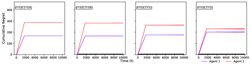
Figure 7: Cumulative regret for different context dimensions in Scenario S4.

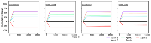
Figure 8: Cumulative regret for different number of agents and arms in Scenario S5.

References

• Abbasi-Yadkori et al. (2011) Abbasi-Yadkori, Y., D. Pál, and C. Szepesvári (2011). Improved algorithms for linear stochastic bandits. Advances in neural information processing systems 24, 2312–2320.
• Abdulkadiroğlu et al. (2005) Abdulkadiroğlu, A., P. A. Pathak, A. E. Roth, and T. Sönmez (2005). The boston public school match. American Economic Review 95(2), 368–371.
• Abdulkadiroğlu and Sönmez (1999) Abdulkadiroğlu, A. and T. Sönmez (1999). House allocation with existing tenants. Journal of Economic Theory 88(2), 233–260.
• Almalis et al. (2014) Almalis, N. D., G. A. Tsihrintzis, and N. Karagiannis (2014). A content based approach for recommending personnel for job positions. In IISA 2014, The 5th International Conference on Information, Intelligence, Systems and Applications, pp.  45–49. IEEE.
• Atila et al. (2005) Atila, A., P. A. Pathak, and A. E. Roth (2005). The new york city high school match. In American Economic Review, Papers and Proceedings, Volume 95.
• Aziz et al. (2021) Aziz, H., P. Biró, and M. Yokoo (2021). Matching market design with constraints. Technical report, Tech. rep., UNSW Sydney.
• Bastani and Bayati (2020) Bastani, H. and M. Bayati (2020). Online decision making with high-dimensional covariates. Operations Research 68(1), 276–294.
• Cen and Shah (2021) Cen, S. H. and D. Shah (2021). Regret, stability, and fairness in matching markets with bandit learners. arXiv preprint arXiv:2102.06246.
• Chen et al. (2021) Chen, H., W. Lu, and R. Song (2021). Statistical inference for online decision making: In a contextual bandit setting. Journal of the American Statistical Association 116(533), 240–255.
• Chen et al. (2021) Chen, X., D. Simchi-Levi, and Y. Wang (2021). Privacy-preserving dynamic personalized pricing with demand learning. Management Science.
• Dai and Jordan (2021a) Dai, X. and M. I. Jordan (2021a). Learning in multi-stage decentralized matching markets. Advances in Neural Information Processing Systems 34.
• Dai and Jordan (2021b) Dai, X. and M. I. Jordan (2021b). Learning strategies in decentralized matching markets under uncertain preferences. Journal of Machine Learning Research 22(260), 1–50.
• Das and Kamenica (2005) Das, S. and E. Kamenica (2005). Two-sided bandits and the dating market. In IJCAI, Volume 5, pp.  19. Citeseer.
• Gale and Shapley (1962) Gale, D. and L. S. Shapley (1962). College admissions and the stability of marriage. The American Mathematical Monthly 69(1), 9–15.
• Guo et al. (2016) Guo, S., F. Alamudun, and T. Hammond (2016). Résumatcher: A personalized résumé-job matching system. Expert Systems with Applications 60, 169–182.
• Gusfield and Irving (1989) Gusfield, D. and R. W. Irving (1989). The stable marriage problem: structure and algorithms. MIT press.
• Jagadeesan et al. (2021) Jagadeesan, M., A. Wei, Y. Wang, M. I. Jordan, and J. Steinhardt (2021). Learning equilibria in matching markets from bandit feedback. Advances in Neural Information Processing Systems 34.
• Kamecke (1992) Kamecke, U. (1992). Two sided matching: A study in game-theoretic modeling and analysis. JSTOR.
• Knuth (1997) Knuth, D. E. (1997). Stable marriage and its relation to other combinatorial problems: An introduction to the mathematical analysis of algorithms, Volume 10. American Mathematical Soc.
• Kojima et al. (2018) Kojima, F., A. Tamura, and M. Yokoo (2018). Designing matching mechanisms under constraints: An approach from discrete convex analysis. Journal of Economic Theory 176, 803–833.
• Lattimore and Szepesvári (2020) Lattimore, T. and C. Szepesvári (2020). Bandit algorithms. Cambridge University Press.
• Li et al. (2010) Li, L., W. Chu, J. Langford, and R. E. Schapire (2010). A contextual-bandit approach to personalized news article recommendation. In Proceedings of the 19th international conference on World Wide Web, pp.  661–670.
• Li et al. (2023) Li, Y., G. Cheng, and X. Dai (2023). Double matching under complementary preferences. arXiv preprint arXiv:2301.10230.
• Li et al. (2021) Li, Y., C.-H. Wang, and G. Cheng (2021). Online forgetting process for linear regression models. In International Conference on Artificial Intelligence and Statistics, pp.  217–225. PMLR.
• Liu et al. (2020) Liu, L. T., H. Mania, and M. I. Jordan (2020). Competing bandits in matching markets. In International Conference on Artificial Intelligence and Statistics, pp.  1618–1628. PMLR.
• Liu et al. (2021) Liu, L. T., F. Ruan, H. Mania, and M. I. Jordan (2021). Bandit learning in decentralized matching markets. Journal of Machine Learning Research 22(211), 1–34.
• Lokhandwala and Cai (2018) Lokhandwala, M. and H. Cai (2018). Dynamic ride sharing using traditional taxis and shared autonomous taxis: A case study of nyc. Transportation Research Part C: Emerging Technologies 97, 45–60.
• Luckett et al. (2019) Luckett, D. J., E. B. Laber, A. R. Kahkoska, D. M. Maahs, E. Mayer-Davis, and M. R. Kosorok (2019). Estimating dynamic treatment regimes in mobile health using v-learning. Journal of the American Statistical Association.
• Min et al. (2022) Min, Y., T. Wang, R. Xu, Z. Wang, M. I. Jordan, and Z. Yang (2022). Learn to match with no regret: Reinforcement learning in markov matching markets. arXiv preprint arXiv:2203.03684.
• Mine et al. (2013) Mine, T., T. Kakuta, and A. Ono (2013). Reciprocal recommendation for job matching with bidirectional feedback. In 2013 Second IIAI International Conference on Advanced Applied Informatics, pp.  39–44. IEEE.
• Nguyen and Vohra (2019) Nguyen, T. and R. Vohra (2019). Stable matching with proportionality constraints. Operations Research 67(6), 1503–1519.
• Qi et al. (2020) Qi, Z., D. Liu, H. Fu, and Y. Liu (2020). Multi-armed angle-based direct learning for estimating optimal individualized treatment rules with various outcomes. Journal of the American Statistical Association 115(530), 678–691.
• Roth (1984) Roth, A. E. (1984). The evolution of the labor market for medical interns and residents: a case study in game theory. Journal of political Economy 92(6), 991–1016.
• Roth (1986) Roth, A. E. (1986). On the allocation of residents to rural hospitals: a general property of two-sided matching markets. Econometrica: Journal of the Econometric Society, 425–427.
• Roth (2008) Roth, A. E. (2008). Deferred acceptance algorithms: History, theory, practice, and open questions. international Journal of game Theory 36(3), 537–569.
• Sankararaman et al. (2020) Sankararaman, A., S. Basu, and K. A. Sankararaman (2020). Dominate or delete: Decentralized competing bandits with uniform valuation. arXiv preprint arXiv:2006.15166.
• Sarkar (2021) Sarkar, S. (2021). Bandit based centralized matching in two-sided markets for peer to peer lending. arXiv preprint arXiv:2105.02589.
• Shi et al. (2022) Shi, C., R. Wan, G. Song, S. Luo, R. Song, and H. Zhu (2022). A multi-agent reinforcement learning framework for off-policy evaluation in two-sided markets. arXiv preprint arXiv:2202.10574.
• Shi et al. (2022) Shi, C., X. Wang, S. Luo, H. Zhu, J. Ye, and R. Song (2022). Dynamic causal effects evaluation in a/b testing with a reinforcement learning framework. Journal of the American Statistical Association (just-accepted), 1–29.
• Shi et al. (2022) Shi, C., S. Zhang, W. Lu, and R. Song (2022). Statistical inference of the value function for reinforcement learning in infinite-horizon settings. Journal of the Royal Statistical Society Series B 84(3), 765–793.
• Sutton and Barto (2018) Sutton, R. S. and A. G. Barto (2018). Reinforcement learning: An introduction. MIT press.
• Vershynin (2018) Vershynin, R. (2018). High-dimensional probability: An introduction with applications in data science, Volume 47. Cambridge university press.
• Vial et al. (2021) Vial, D., S. Shakkottai, and R. Srikant (2021). Robust multi-agent multi-armed bandits. In Proceedings of the Twenty-second International Symposium on Theory, Algorithmic Foundations, and Protocol Design for Mobile Networks and Mobile Computing, pp.  161–170.
• Wainwright (2019) Wainwright, M. J. (2019). High-dimensional statistics: A non-asymptotic viewpoint, Volume 48. Cambridge University Press.
• Wang et al. (2020) Wang, C.-H., Z. Wang, W. W. Sun, and G. Cheng (2020). Online regularization for high-dimensional dynamic pricing algorithms. arXiv preprint arXiv:2007.02470.
• Wang et al. (2021) Wang, Y., X. Chen, X. Chang, and D. Ge (2021). Uncertainty quantification for demand prediction in contextual dynamic pricing. Production and Operations Management 30(6), 1703–1717.
• Zap et al. (2018) Zap, L., J. van Breugel, D. Bakker, and S. Bels (2018). Swiping right vs. finding mr. right: Facebook attempts to reinvent online dating. In New media and digital culture.