Università degli Studi dell’Insubria
DIPARTIMENTO DI SCIENZA E ALTA TECNOLOGIA
Ph.D. Thesis / Dissertation
The Renormalization Scale Setting Problem in QCD
Author:
Leonardo Di Giustino
Advisor:
Prof. Philip G. Ratcliffe
Chair of the Doctoral Programme:
Prof. Giuliano Benenti
XXXIV CICLO - January 2022
Glossary
- AF
-
asymptotic freedom.
- BLM
-
Brodsky-Lepage-Mackenzie.
- BSM
-
beyond standard model.
- CSR
-
commensurate scale relation.
- CSS
-
conventional scale setting.
- EW
-
electroweak.
- FAC
-
fastest apparent convergence principle.
- GCR
-
generalized Crewther relation.
- GM–L
-
Gell-Mann–Low.
- GUT
-
grand unified theory.
- HQ
-
heavy quark.
- iCF
-
intrinsic conformality.
- IR
-
infrared.
- mMOM
-
minimal momentum-subtraction scheme.
- MOM
-
momentum-subtraction scheme.
- MS
-
minimal-subtraction scheme.
-
modified minimal-subtraction scheme.
- NP
-
new physics.
- OPT
-
optimized perturbation theory.
- pQCD
-
perturbative quantum chromodynamics.
- PMC
-
principle of maximum conformality.
- PMCa
-
alternative principle of maximum conformality scale-setting.
- PMCm
-
multi-scale principle of maximum conformality scale-setting.
- PMCs
-
single-scale principle of maximum conformality scale-setting.
- PMC∞
-
infinite-order scale-setting using the principle of maximum conformality.
- PMS
-
principle of minimal sensitivity.
- RG
-
renormalization group.
- RGE
-
renormalization group equations.
- RS
-
renormalization scheme.
- RSS
-
renormalization scale setting.
- SM
-
standard model.
- UV
-
ultraviolet.
- V-scheme
-
scheme of the static potential between two heavy quarks.
- xRGE
-
extended renormalization group equations.
“In the perspective of a theory unifying all the interactions, electromagnetic, weak and strong nuclear, such as a so-called grand unified theory or GUT, we are constrained to apply the same scale-setting procedure in all sectors of the theory.”
Introduction
A key issue in making precise predictions in QCD is the uncertainty in setting the renormalization scale in order to determine the correct running coupling in the perturbative expansion of a scale invariant quantity. Other quantities such as the top and Higgs mass uncertainty, the strong coupling uncertainty also affect the theoretical predictions for perturbative QCD, but one of the most important sources of error is given by the renormalization scale and scheme ambiguities. These scale and scheme ambiguities are an important source of uncertainties for predictions in many fundamental processes in perturbative QCD, such as the gluon fusion in Higgs production [1], or bottom-quark production [2], which are essential for the physics investigated at the Large Hadron Collider (LHC) and at future colliders.
Precise predictions are crucial for both standard model (SM) and beyond the standard model (BSM) physics, in order to enhance sensitivity to new physics (NP) at colliders.
In principle, an infinite perturbative series is void of this issue, given the scheme and scale invariance of the entire physical quantities [3, 4, 5, 6, 7], in practice perturbative corrections are known up to a certain order of accuracy and scale invariance is only approximated in truncated series leading to so-called scheme and scale ambiguities [8, 9, 10, 11, 12, 13, 14, 15, 16, 17, 18]. On one hand, according to the conventional practice or conventional scale setting (CSS), this problem cannot be avoided and is responsible for part of the theoretical errors. Using the CSS approach the renormalization scale is set to the typical scale of a process Q, and errors are estimated by varying the scale over a range of two . This method gives predictions with large theoretical uncertainties comparable with the calculated order correction. Moreover, this procedure leads to results that depend on the renormalization scheme and on the initial scale choice, to a perturbative series that diverges as [19], and does not agree with QED. Moreover, in several processes there is more than one typical scale and results can be significantly different for perturbative calculations according to the different choices of scale [20].
On the other hand, some strategies for the optimization of the truncated expansion have been proposed, such as the Principle of Minimal Sensitivity (PMS) proposed by Stevenson [13, 12, 11, 10], the Fastest Apparent Convergence (FAC) criterion introduced by Grunberg [14, 15, 16]. These are procedures commonly in use for scale setting in perturbative QCD together with the CSS and an introduction to these methods can also be found in Refs. [21, 22]. However, as shown in Refs. [21], these methods not only have the same difficulties of CSS, but they also lead to incorrect and unphysical results [23] in particular kinematic regions.
In general a scale-setting procedure is considered reliable if it preserves important self-consistency requirements. All Renormalization Group properties such as: uniqueness, reflexivity, symmetry, and transitivity should be preserved also by the scale-setting procedure in order to be generally applied [24]. Other requirements are also suggested by known tested theories, by the convergence behavior of the series and also for phenomenological reasons or scheme independence.
It has been shown how all the theoretical requirements for a reliable scale-setting procedure can be satisfied at once, leading to accurate results by using the PMC (the Principle of Maximum Conformality [25, 26, 27]). This method is the generalization and extension of the original Brodsky-Lepage-Mackenzie (BLM) method [17] to all orders and to all observables. The primary purpose of the PMC method is to solve the scale-setting ambiguity, it has been extended to all orders [28, 29] and it determines the correct running coupling and the correct momentum flow according to RGE invariance [30, 31]. This leads to results that are invariant respect to the initial renormalization scale in agreement with the requirement of scale invariance of an observable in pQCD [21]. This method provides a systematic way to eliminate renormalization scheme and scale ambiguities from first principles by absorbing the terms that govern the behavior of the running coupling via the renormalization group equation. Thus, the divergent renormalon terms cancel, which improves convergence of the perturbative QCD series. Furthermore, the resulting PMC predictions do not depend on the particular scheme used, thereby preserving the principles of renormalization group invariance [24, 30]. The PMC procedure is also consistent with the standard Gell-Mann–Low method in the Abelian limit, [32]. Moreover, in a theory of unification of all forces, electromagnetic, weak and strong interactions, such as Grand Unified theories, one cannot simply apply a different scale-setting or analytic procedure to different sectors of the theory. The PMC offers the possibility to apply the same method in all sectors of a theory, starting from first principles, eliminating the renormalon growth, the scheme dependence, the scale ambiguity, and satisfying the QED Gell-Mann-Low scheme in the zero-color limit .
We show in this thesis, how the implementation at all orders of the PMC simplifies in many cases by identifying only the -terms at each order of accuracy due to the presence of a new property of the perturbative corrections: the intrinsic conformality (iCF). First we recall that there is no ambiguity in setting the renormalization scale in QED. The standard Gell-Mann-Low scheme determines the correct renormalization scale identifying the scale with the virtuality of the exchanged photon [4]. For example, in electron-muon elastic scattering, the renormalization scale is the virtuality of the exchanged photon, i.e. the spacelike momentum transfer squared . Thus
| (1) |
where
From Eq. 3.8 it follows that the renormalization scale can be determined by the -term at the lowest order. This scale is sufficient to sum all the vacuum polarization contributions into the dressed photon propagator, both proper and improper, at all orders. Again in QED, considering the case of two-photon exchange, a new different scale is introduced in order to absorb all the -terms related to the new subprocess into the scale. Also in this case the scale can be determined by identifying the lowest-order -term alone. This term identifies the virtuality of the exchanged momenta causing the running of the scale in that subprocess. This scale again would sum all the contributions related to the -function into the renormalization scale and no further corrections need to be introduced into the scale at higher orders. Given that the pQCD and pQED predictions match analytically in the limit where (see Ref. [32]), we extend the same procedure to pQCD. In fact, in many cases in QCD the terms alone can determine the pQCD renormalization scale at all orders [33] eliminating the renormalon contributions . Although in non-Abelian theories other diagrams related to the three- and four-gluon vertices arise, these terms do not necessarily spoil this procedure. In fact, in QCD, the terms arising from the renormalization of the three-gluon or four-gluon vertices as well as from gluon wavefunction renormalization determine the renormalization scales of the respective diagrams and no further corrections to the scales need to be introduced at higher orders. In conclusion, if we focus on a particular class of diagrams we can fix the PMC scale by determining the -term alone and we show this to be connected to the general scheme and scale invariance of an observable in a gauge theory.
This thesis is organized as follows: in section I we introduce QCD as a gauge theory based on the local symmetry; in section II we give a description of the renormalization group equations and their extended version, starting from the renormalization procedure of the strong coupling and its renormalization scale dependence; in section III we present the state of the art for the renormalization scale setting problem in QCD, introducing the basic concepts of scale setting procedures in use at present: conventional scale setting (CSS), FAC-scale setting, PMS-scale setting and BLM scale setting, highlighting their basic features and showing some important physical results; in section IV we describe the PMC approach; in section V we introduce the newly developed method PMC∞ and its new features; we show results for the application of the PMC∞ to the event-shape variables: thrust and C-parameter comparing the results under the CSS and the PMC∞ methods; in section VI we apply the PMC∞ to thrust in the perturbative conformal window of QCD and we investigate the QED limit of the QCD thrust calculations; in section VII we show a novel method to determine the strong coupling and its behavior over a wide range of scales, from a single experiment at a single scale, using the event shape variable results; in section VIII we apply the PMC/PMC∞ to a multi-renormalization scale process: heavy-quark pair production at threshold, comparing results in different schemes and taking the QED limit of the QCD calculations.
This thesis mostly summarizes results published in the following articles or conference proceedings:
-
•
L. Di Giustino, Stanley J. Brodsky, Xing-Gang Wu and Sheng-Quan Wang, PMC∞: Infinite-Order Scale-Setting method using the Principle of Maximum Conformality and preserving the Intrinsic Conformality; Proceedings of the conference RADCOR 2021, arXiv:2110.05171 [hep-ph].
-
•
L. Di Giustino, Francesco Sannino, Sheng-Quan Wang and Xing-Gang Wu, Thrust Distribution for 3-Jet Production from Annihilation within the QCD Conformal Window and in QED, Physics Letters B 823C (2021) 136728; arXiv:2104.12132[hep-ph];
-
•
L. Di Giustino, Stanley J. Brodsky, Sheng-Quan Wang and Xing-Gang Wu, Infinite-order scale-setting using the principle of maximum conformality: A remarkably efficient method for eliminating renormalization scale ambiguities for perturbative QCD, Phys.Rev.D 102 (2020) 1, 014015: arXiv: 2002.01789[hep-ph];
-
•
Sheng-Quan Wang, Stanley J. Brodsky, Xing Gang Wu, L. Di Giustino and Jian-Ming Shen, Renormalization scale setting for heavy quark pair production in annihilation near the threshold region, Phys.Rev.D 102 (2020) 1, 014005: arXiv: 2002.10993[hep-ph];
-
•
Sheng-Quan Wang, Stanley J. Brodsky, Jian-Ming Shen, Xing-Gang Wu and L. Di Giustino A Novel Method for the Precise Determination of the QCD Running Coupling from Event Shapes Distributions in Electron-Positron Annihilation, Phys. Rev. D 100 (2019) 9, 094010 : arXiv:1908.00060[hep-ph];
-
•
Sheng-Quan Wang, Stanley J. Brodsky, Xing-Gang Wu, L. Di Giustino Thrust Distribution in Electron-Positron Annihilation using the Principle of Maximum Conformality, Phys. Rev. D 99 (2019) 11, 114020: arXiv: 1902.01984[hep-ph];
-
•
X. D. Huang, J. Yan, H. H. Ma, L. Di Giustino, J. M. Shen, X. G. Wu and S. J. Brodsky, Detailed Comparison of Renormalization Scale-Setting Procedures based on the Principle of Maximum Conformality, arXiv:2109.12356 [hep-ph];
-
•
Sheng-Quan Wang, Chao-Qin Luo, Xing-Gang Wu, Jian-Ming Shen, Leonardo Di Giustino, New analyses of event shape observables in electron-positron annihilation and the determination of running behavior in perturbative domain, arXiv:2112.06212 [hep-ph];
Chapter 1 Quantum Chromodynamics
1.1 Introduction
Quantum Chromodynamics is the theory of the strong interaction, which describes how elementary constituents such as quarks and gluons interact in order to bind together and form hadrons. In particular, the theory exhibits the symmetries observed experimentally and it explains why quarks interact strongly at low energies and weakly in processes at large momentum transfer, where quarks appear to be almost free.
Despite the many successful achievements, there are still several problems that need to be solved in order to test the theory to the highest precision. In particular, the confinement mechanism still remains unexplained, though some evidence of such phenomenon has been obtained in recent years by investigating gauge theories on the lattice and by studying the topology of the non-Abelian gauge theories. In order to overcome this obstacle, several alternative approaches have also been proposed, which so far unfortunately are not completely void of ambiguities and lead to results that are rather model dependent. The non-perturbative region is in fact affected by the peculiar infrared (IR) dynamics, which involves mechanisms like hadronization, soft radiation and confinement. In particular, in the IR region the behavior of the strong coupling is not yet predictable or explained in QCD. Recent studies of light front holographic QCD (LFHQCD) (i.e. AdS/CFT theory) suggest the presence of a finite limit of the coupling at zero momentum, which means the presence of an interacting fixed point in the -function. This hypothesis has not been rejected by comparison with experimental data and the behavior of the coupling seems to be in agreement. At the moment the AdS/CFT correspondence with QCD is still under investigation and the LFHQCD can be considered only as a model or as an “ansatz” for the non-perturbative region of QCD. Despite the lack of a perturbative expansion at low energies, there are still several strong theorems that hold and that can be used to relate processes with analogous characteristics in the non-perturbative region and model parameters can be constrained by fits to data. Thus, if on one hand the dynamics at long distances is not yet totally revealed, on the other hand the dynamics at high energies reached its apex with the discovery of asymptotic freedom (AF), which perfectly explains experimental evidence of the weakly interacting partons inside hadrons at high momentum transfer. The perturbative nature of QCD at short distances is still affected by errors due to uncertainties, which in several cases can spoil the theoretical predictions and which are related to both the confining nature of the strong forces and the renormalization scale and scheme ambiguities. The latter are the main sources of errors in many processes where QCD corrections can be calculated perturbatively. In order to make reliable theoretical predictions and improve the precision, it is crucial to eliminate the scale and scheme ambiguities in order to improve the theoretical calculations in QCD enhancing the sensitivity to any possible signal of new physics (NP) at the large hadron collider (LHC). Furthermore, QCD is the most complex gauge theory we have ever dealt with, it represents the most difficult sector of the Standard Model (SM) for quantitatively predictions. In fact, if in the electroweak (EW) sector, perturbation theory is always applicable, given the particular weak nature of the interaction at energies accessible in accelerators or in weak decays involving leptons and vector bosons, this is not always possible in QCD since the coupling in a wide range of scales and quarks cannot be observed as real states. Thus the complex nature of QCD can only be investigated by comparing its predictions with all possible results from different experiments in different kinematic regions. Given the vast variety of the phenomena and phenomenological applications, QCD is currently still a field of great interest and under continuous and active investigation.
1.2 The flavor symmetry:
Neutron, proton, pions and the other particles listed in the Particle Data Group (PDG) [34] tables are classified as hadrons and have in common the particular property of interacting via the strong interaction. All these particles can be simply classified using global symmetries, in particular the symmetry. This was originally discovered by Gell-Mann and Neeman with the quarks up, down, strange (u, d, s) and was later expanded to include the quarks charm (c), bottom (b) and top (t). These symmetries apply, following the Gell-Mann and Zweig approach, starting from the assumption that light hadrons are formed by quarks, respectively three for baryons and two (a quark and an antiquark) for mesons. Quarks are fermions of spin 1/2 divided into six flavors. Three quarks, u, c, t, have charge , while d, s, b have a charge of . Following the original idea of the isospin symmetry of Heisenberg for the states of the nucleon, Gell-Mann introduced the group for the quarks: u, d, s. The symmetry applies straightforwardly assuming first that the three light quarks u, d, s transform as a fundamental representation of the flavor symmetry group . All other particles formed by the u, d, s quarks can be classified as higher representations of the group, which can be generated by taking multiple products of the fundamental representation:
| (1.1) |
The group is a rank 2 Lie group and its representations are identified with two quantum numbers: by convention we take the third component of isospin and the hypercharge . The two quantum numbers strangeness and hypercharge are not independent, but are related by the Gell-Mann and Nishijma formula:
where , with the baryon number, which for all quarks has the value , is the strangeness and the electric charge. In this model, we expect mesons and light baryons to be classified according to the following representations:
| (1.2) |
The symmetry of Gell-Mann and Neeman predicts that mesons are arranged in terms of octets and singlets, with baryons in octets, decuplets and singlets. The fact that this simple representation can in fact classify the lightest mesons and baryons present in nature, was a remarkable achievement.
At present six different flavors of quarks are known, and in principle, one could think of generalizing to . Unfortunately, the large differences among the heavier quark states, break the global symmetry strongly. In contrast, the original symmetry of the light quarks is nearly conserved, given that the u, d, s quarks have approximately the same masses. This justifies the approximation of the quasi-conserved chiral symmetries, under which the left-handed and right-handed fields transform independently of each other. Such chiral symmetries are given by the invariance of the Lagrangian under the group or considering a better approximation, by the group , involving only the up and down quarks, which can be actually considered massless ().
1.3 Hints for color
The discovery of the baryon in 1951 [35] provided a first indication of the existence of a new degree of freedom necessary to antisymmetrize its wavefunction. In fact, the particle is in a fundamental state with all spins aligned along the same direction , which leads to a symmetric wavefunction. This is in contrast with the Pauli exclusion principle and Fermi-Dirac statistics, given that baryons have semi-integer spin. In order to overcome this inconsistency, a new quantum number was introduced: color, with at least number of colors and with each quark having a color index . Thus, according to this assumption the wavefunction can be antisymmetric:
| (1.3) |
Other experimental evidence for color was provided by measurements of the decay width of the neutral pion, and by the ratio that showed a neat proportionality. These experimental hints were also supported by other theoretical indications like the anomaly cancellation and the problem of the meson mass.
1.4 Quarks and gluons
The “quark model” introduced by Gell-Mann, comprehensively explains the spectrum of hadronic states and in particular the spectra of states containing heavy quarks such as charm and bottom: charmonium, bottomonium respectively and also D and B mesons. The charmonium, bottomonium states appear as resonances of and quark states. Taking into account the reduced mass difference, these are in fact similar to the states of positronium () and can be obtained assuming that the heavy quarks interact via a non-relativistic potential that at short-distances has the characteristics of an effective Coulomb-like static potential, while at large-distances diverges linearly according to the confinement mechanism. For the sake of completeness, in order to complement the description of the interaction of heavy quarks, relativistic and pQCD corrections should be also taken into account. It was also found that, in processes with large momentum transfer, hadrons appear to be made up of almost free elementary constituents (i.e. weakly interacting with each other) called partons by Feynman.
After careful analysis and measurements of charges and spins, Feynman’s partons were identified with Gell-Mann’s quarks. It was deduced that these values are in agreement with those of the quark model. In particular, at the moment we know of 6 quark flavors: namely, and where each flavor also corresponds to three different states of color . Quarks are then elementary particles that interact via strong forces exchanging other massless particles, i.e. gluons. However, quarks have never been observed as free particles in laboratories, so they cannot be represented as asymptotic states. They only exist as elementary constituents of hadrons, wherein they are confined. Moreover, also real states of single gluons cannot be directly observed. Gluons are the bosons that convey the strong forces inside hadrons analogously to photons in QED, but unlike photons they carry the color charge. In fact, they exist in the octet configuration or adjoint representation. In this picture, quarks and gluons are carriers of the color quantum number, while baryons and mesons are colorless particles. This means that all hadrons are singlets under rotations in the color space and cannot exchange long range gluons. In order to avoid the existence of extra unobserved hadronic states, to therefore satisfy hadron spectroscopy, one must postulate furthermore that all asymptotic states are colorless. This assumption is known as the hypothesis of confinement; in fact, it implies the non-observability of free quarks and gluons, which excludes the color singlet gluon state.
1.5 Gauge theories
QCD is a non-Abelian gauge theory, i.e. a Lagrangian quantum field theory with the gauge symmetry given by the invariance of the Lagrangian under the local special unitary Lie group transformations. In general, gauge theories satisfy two fundamental requirements: invariance under the particular gauge group, which for the Standard Model is and renormalizability. These two requirements lead to a theory that is symmetric under the local transformation of the particular special unitary group and under the renormalization group equations (RGE). The groups and are non-Abelian special unitary groups related to the strong and weak forces. The is the Abelian group of hypercharge, which leads to QED after the spontaneous symmetry breaking (SSB) mechanism. Lie groups have the following Standard representations:
where are real parameters and Hermitian traceless matrices defined as group generators. Special unitary groups have a total number of generators , where “” is the dimension of the fundamental representation of the group, and generators are diagonal. The algebra of Lie groups is set by the commutation relations of the generators:
| (1.4) |
and
| (1.5) |
where and are total antisymmetric tensors and are the structure constants of the group, while the with and the with are the adjoint representations of the and group given by the Pauli and the Gell-Mann matrices respectively.
1.6 The QCD Lagrangian
The QCD Lagrangian can be derived from the Yang-Mills Lagrangian by adding all flavor contributions. The Yang-Mills Lagrangian is itself a gauge invariant Lagrangian under local special-unitary transformations:
| (1.6) |
Local gauge matrices, , can be parametrized using the form:
| (1.7) |
where is the coupling constant, which is related to by: and are the group generators of , which are given by the Gell-Mann matrices:
| (1.8) |
The are arbitrary parameters depending on space-time coordinates. In order to preserve the gauge invariance locally, a new definition of the derivative occurs, the covariant derivative:
| (1.9) |
where is the fermionic field in its fundamental representation of the group , with and the flavor and color indices respectively, and:
| (1.10) |
the eight gauge fields relative to the eight gluons with . Following these considerations we can write the QCD Lagrangian as:
| (1.11) |
where the gluon field strength tensor is given by:
| (1.12) | |||||
with
| (1.13) |
Due to the non-commutative nature of , the trace of the field strength tensor introduces gluon cubic and quartic self interactions, which is the main difference between QCD and QED. These interactions are particularly important in the calculation of the -function and lead to a fundamental property of QCD: asymptotic freedom. Eq. 1.11 is still missing two terms and , respectively the Lagrangians for the gauge fixing and ghost terms, which must be introduced for consistency (for a review see Ref. [36]). However, these terms do not introduce extra real final or initial particle states, but fictitious particles; namely ghosts, which occur only in loop integration.
1.7 Quark states and
According to the Lagrangian in Eq. 1.11, the strong force preserves the flavor quantum number. The interactions that change flavor stem from weak interactions. In fact, flavor-changing transitions among different quarks have a lower intensity with respect to flavor conserving interactions. Moreover, intermediate bosons of the electroweak interactions (, , ), do not couple via strong forces or to color charges. Thus, the color symmetry is well preserved by the strong forces and it can be considered the perfect candidate for the QCD symmetry group. Moreover, QCD includes the following features:
-
•
color is an exact symmetry;
-
•
;
-
•
quarks and antiquarks have different fundamental representations: , this leads to a complex representation;
-
•
hadrons are colorless particles, so they must be represented as color singlets;
-
•
asymptotic freedom.
These conditions exclude other groups, but lead straightforwardly to the group symmetry. Assuming the fundamental representations for quarks and antiquarks, and respectively, we can determine the other possible states considering multiple combinations of quarks and/or antiquarks:
| (1.14) |
Simple color singlets result from and and lead to mesons and baryons respectively. Recently other unstable particles assumed to be tetraquarks (e.g. X(3872)) and pentaquarks (e.g. (1540)) [37] have been observed by Belle, D, BaBar and LHCb, while there is no evidence for a six quark state. A first six quark state, namely hexaquark, was introduced by Jaffe (H-dibaryon [38]) and recently by Farrar (sexaquark [39]). Actually color representations for mesons and baryons are not the only color singlets possible that can be realized with multiple combinations of quarks and antiquarks. In fact, color singlets can also be formed considering the combinations: . Tetraquark and pentaquark states are both unstable, while the sexaquark is claimed to be stable. However, it is still under investigation if these novel quark states are simple bound states or molecules.
Chapter 2 The Renormalization Group
2.1 Renormalization
Renormalization is a procedure that applied quantum field theories (QFT) in order to cancel an infinite number of ultraviolet (UV) singularities that arise in loop integration absorbing them into a finite number of parameters entering the Lagrangian, like the mass or coupling constant and fields. This procedure starts from the assumption that the variables entering the Lagrangian are not the effective quantities measured in experiments, but are unknown functions affected by singularities. The origin of the ultraviolet singularities is often interpreted as a manifestation that a QFT is a low-energy effective theory of a more fundamental yet unknown theory.
The use of regularization UV cut-offs shields the very short distance domain, where the perturbative approach to QFT ceases to be valid.
Once the coupling has been renormalized to a measured value and at a given energy scale, the effective coupling is no longer sensitive to the ultraviolet (UV) cut-off nor to any unknown phenomena arising beyond this scale. Thus, the scale dependence of the coupling can be well understood formally and phenomenologically. Actually gauge theories are affected not only by UV, but also by infrared (IR) divergencies. The cancellation of the latter is guaranteed by the Kinoshita - Lee - Nauenberg (KLN) theorem [40, 41].
Considering first the Lagrangian of a massless theory, which is free from any particular scale parameter, in order to deal with these divergences a regularization procedure is introduced. Referring to the dimensional regularization procedure [42, 43, 44], one varies the dimension of the loop integration, and introduces a scale in order to restore the correct dimension of the coupling.
In order to determine the renormalized gauge coupling, we consider the quark-quark-gluon vertex and its loop corrections. UV-divergences arise from loop integration for higher order contributions for both the external fields and the vertex. The renormalization constants are related by:
| (2.1) |
where is the coupling renormalization factor, is the vertex renormalization constant and and are:
the renormalization constants for gluon and quark fields respectively. The superscript indicates the renormalized field. The renormalization factors in dimensional regularization are given by:
| (2.2) | |||||
| (2.3) | |||||
| (2.4) |
where is the regulator parameter for the UV-ultraviolet singularities. By substitution, we have that the UV divergence :
| (2.5) |
with
| (2.6) |
The singularities related to the UV poles are subtracted out by a redefinition of the coupling. In the scheme, the renormalized strong coupling is related to the bare coupling by:
| (2.7) |
In the minimal subtraction scheme () only the pole related to the UV singularity is subtracted out. A more suitable scheme is [45, 46, 47], where also the constant term is subtracted out. Different schemes can also be related by scale redefinition, e.g. . Thus, the renormalization procedure depends both on the particular choice of the scheme and on the subtraction point .
Hence, even though there are no dimensionful parameters in the initial bare Lagrangian, a mass scale is acquired during the renormalization procedure. The emergence of from a Lagrangian without any explicit scale is called dimensional transmutation [48]. The value of is arbitrary and is the momentum at which the UV divergences are subtracted out. Hence is called the subtraction point or renormalization scale. Thus, the definition of the renormalized coupling depends at the same time on the chosen scheme, and on the renormalization scale .
However, different schemes and scales can be related according to the so-called extended renormalization group equations, which we will introduce in the following sections. Given the perturbative nature of the theory, these relations are known up to a certain level of accuracy and the truncated formulas are responsible for an important source of uncertainties: the scheme and scale ambiguities.
2.2 The running coupling constant
In this section we will discuss the dependence of the strong coupling on the renormalization scheme (RS) and scale () and we will show how this dependence can be controlled by means of the renormalization group equations (RGE). The strong coupling , is a fundamental parameter of the SM theory and determines the strength of the interactions among quarks and gluons in quantum chromodynamics (QCD). As shown in the previous section, its value depends on the renormalization scale (i.e. the subtraction point). In order to understand hadronic interactions, it is necessary to determine the magnitude of the coupling and its behavior over a wide range of values, from low to high energy scales. Long and short distances are related to low and high energies respectively. In the high energy region the strong coupling has an asymptotic behavior and QCD becomes perturbative, while in the region of low energies, e.g. at the proton mass scale, the dynamics of QCD is affected by processes such as quark confinement, soft radiation and hadronization. In the first case experimental results can be matched with theoretical calculations and a precise determination of the depends both on experimental accuracy and on theoretical errors. In the latter case experimental results are difficult to achieve and theoretical predictions are affected by the confinement and hadronization mechanisms, which are rather model dependent. Various processes also involve a precise knowledge of the coupling in both the high and low momentum transfer regions and in some cases calculations must be improved with electroweak (EW) corrections. Thus, the determination of the QCD coupling over a wide range of energy scales is a crucial task in order to achieve results and to test QCD to the highest precision. Theoretical uncertainties in the value of contribute to the total theoretical uncertainty in the physics investigated at the Large Hadron Collider (LHC), such as the Higgs sector, e.g. gluon fusion Higgs production [1]. The behavior of the perturbative coupling at low-momentum transfer is also fundamental for the scale of the proton mass, in order to understand hadronic structure, quark confinement and hadronization processes. IR effects such as soft radiation and renormalon factorial growth spoil the perturbative nature of the QCD in the low-energy domain. Higher-twist effects can also play an important role. Processes involving the production of heavy quarks near threshold require the knowledge of the QCD coupling at very low momentum scales. Even reactions at high energies may involve the integration of the behavior of the strong coupling over a large domain of momentum scales including IR regions. Precision tests of the coupling are crucial also for other aspects of QCD that are still under continuous investigation, such as the hadron masses and their internal structure. In fact, the strong interaction is responsible for the mass of hadrons in the zero-mass limit of the u, d quarks.
The origin and phenomenology of the behavior of at small distances, where asymptotic freedom appears, is well understood and explained in many textbooks on Quantum Field Theory and Particle Physics.
Numerous reviews exist; see e.g. Refs. [49, 50]. However, standard explanations often create an apparent puzzle, as will be addressed in this thesis. Other questions remain even in this well understood regime: a significant issue is how to identify the scale Q that controls a given hadronic process, especially if it depends on many physical scales. A fundamental requirement, called “renormalization group invariance”, is that physical observables cannot depend on the choice of the renormalization scale and scheme.
In the perturbative regime theoretical predictions are affected by several sources of errors, e.g. the top and Higgs mass uncertainty, the strong coupling uncertainty and the main source of errors is given by the renormalization scale and scheme ambiguity. In this section we discuss the scale and scheme dependence of the effective coupling in QCD.
2.3 The evolution of in perturbative QCD
As shown in the previous section the renormalization procedure is not void of ambiguities. The subtraction of the singularities depends on the subtraction point or renormalization scale and on the renormalization scheme (RS). Observables in physics cannot depend on the particular scheme or scale, given that the theory stems from a conformal Lagrangian. This implies that scale invariance must be recovered imposing the invariance of the renormalized theory under the renormalization group equation (RGE). We discuss in this section the dependence of the renormalized coupling on the scale . As shown in QED by Gell-Mann and Low, this dependence can be described introducing the -function given by:
| (2.8) |
and
| (2.9) |
Neglecting quark masses, the first two -terms are RS independent and they have been calculated in Refs. [51, 52, 53, 54, 55] for the scheme:
where ,
and are the color factors for the gauge group [56].
At higher loops we have that are scheme
dependent and results for are calculated in
Ref. [57]:
in Ref. [58]:
| (2.10) | |||||
and in Ref. [59]:
| (2.11) | |||||
with , and , the Riemann zeta function. Given the renormalizability of QCD, new UV singularities arising at higher orders can be cancelled by redefinition of the same parameter, i.e. the strong coupling. This procedure leads to the renormalization factor:
| (2.12) | |||||
where in the scheme. Given the arbitrariness of the subtraction procedure of including also part of the finite contributions (e.g. the constant for the ), there is an inherent ambiguity for these terms which translates into the RS dependence. In order to solve any truncated Eq. 2.8, this being a first order differential equation, we need an initial value of at a given energy scale . For this purpose we set the initial scale the mass and the value is determined phenomenologically. In QCD the number of colors is set to 3, while , i.e. the number of active flavors, varies with energy scale across quark thresholds.
2.4 One-loop result and asymptotic freedom
When all quark masses are set to zero two physical parameters dictate the dynamics of the theory and these are the numbers of flavors and colors . We determine in this section the exact analytical solution to the truncated Eq. 2.8. Considering the formula :
| (2.13) |
and retaining only the first term:
| (2.14) |
we achieve the solution for the coupling:
| (2.15) |
This solution can be given in the explicit form:
| (2.16) |
This solution relates one known (measured value) of the coupling at a given scale with an unknown value . More conveniently, the solution can be given introducing the QCD scale parameter . At order, this is defined as:
| (2.17) |
which yields the familiar one-loop solution:
Already at the one loop level one can distinguish two regimes of the theory. For the number of flavors larger than (i.e. the zero of the coefficient) the theory possesses an infrared non-interacting fixed point and at low energies the theory is known as non-abelian quantum electrodynamics (non-abelian QED). The high energy behavior of the theory is uncertain, it depends on the number of active flavors and there is the possibility that it could develop a critical number of flavors above which the theory reaches an UV fixed point [60] and therefore becomes safe. When the number of flavors is below the non-interacting fixed point becomes UV in nature and then we say that the theory is asymptotically free.
It is straightforward to check the asymptotic limit of the coupling in the deep UV region:
| (2.18) |
This result is known as asymptotic freedom and it is the outstanding result that has justified QCD as the most accredited candidate for the theory of strong interactions. On the other hand, we have that the perturbative coupling diverges at the scale. This is sometimes referred to as the Landau ghost pole to indicate the presence of a singularity in the coupling that is actually unphysical and indicates the breakdown of the perturbative regime. This itself is not an explanation for confinement, though it might indicate its presence. When the coupling becomes too large the use of a nonperturbative approach to QCD is mandatory in order to obtain reliable results. We remark that the scale parameter is RS dependent and its definition depends on the order of accuracy of the coupling . Considering that the solution at order or is universal, the definition of at the first two orders is usually preferred, i.e. the given at 1-loop by Eq. 2.17 or at 2-loops (see later) by Eq. 2.23 .
2.5 Two-loop solution and the perturbative conformal window
In order to determine the solution for the strong coupling at NNLO, it is convenient to introduce the following notation: , , and , . The truncated NNLO approximation of the Eq. 2.8 leads to the differential equation:
| (2.19) |
An implicit solution of Eq. 2.19 is given by the Lambert function:
| (2.20) |
with: . The general solution for the coupling is:
| (2.21) | |||||
| (2.22) |
We will discuss here the solutions to Eq. 2.19 with respect to the particular initial phenomenological value given by the coupling determined at the mass scale [34].
The signs of and consequently of , depends on the values of the , since the number is set by the theory , we discuss the possible regions varying only the number of flavors . We point out that different regions are defined by the signs of the , that have zeros in , respectively with .
In the range and we have , and the physical solution is given by the branch, while for the solution for the strong coupling is given by the branch. By introducing the phenomenological value , we define a restricted range for the IR fixed point discussed by Banks and Zaks [61]. Given the value , we have that in the range the -function has both a UV and an IR fixed point, while for we no longer have the asymptotically free UV behavior. The two-dimensional region in the number of flavors and colors where asymptotically free QCD develops an IR interacting fixed point is colloquially known as the conformal window of pQCD.
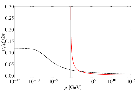
Thus, the actual physical range of a conformal window for pQCD is given by . The behavior of the coupling is shown in Fig. 2.1. In the IR region the strong coupling approaches the IR finite limit, , in the case of values of within the conformal window (e.g. black dashed curve of Fig. 2.1), while it diverges at
| (2.23) |
outside the conformal window given the solution for the coupling with (e.g. the solid red curve of Fig. 2.1). The solution of the NNLO equation for the case , i.e. , can also be given using the standard QCD scale parameter of Eq. 2.23,
| (2.24) | |||||
| (2.25) |
Different solutions can be achieved using different schemes, i.e. different definitions of the scale parameter [62]. We underline that the presence of a Landau “ghost” pole in the strong coupling is only an effect of the breaking of the perturbative regime, including non-perturbative contributions, or using non-perturbative QCD, a finite limit is expected at any [22]. Both solutions have the correct UV asymptotic free behavior. In particular, for the case , we have a negative , a negative and a multi-valued solution, one real and the other imaginary, actually only one (the real) is acceptable given the initial conditions, but this solution is not asymptotically free. Thus we restrict our analysis to the range where we have the correct UV behavior. In general IR and UV fixed points of the -function can also be determined at different values of the number of colors (different gauge group ) and extending this analysis also to other gauge theories [63].
2.6 at higher loops
The 3-loop truncated RG equation 2.8, written using the same normalization of Eq. 2.19 is given by:
| (2.26) |
with .
A straightforward integration of this equation would be hard to invert, as shown in Ref. [62] it is more convenient to extend the approach of the previous section by using the Padé Approximant (PA). The Padé Approximant of a given quantity calculated perturbatively in QCD up to the order , i.e. of the series:
| (2.27) |
is defined as the rational function:
| (2.28) |
whose Taylor expansion up to the order is identical to the original truncated series. The use of the PA makes the integration of Eq. 2.26 straightforward. PA’s may be also used either to predict the next term of a given perturbative expansion, called a Padé Approximant prediction (PAP), or to estimate the sum of the entire series, called Padé Summation. Features of the PA are shown in Ref. [65].
The Padé Approximant () of the 3-loop is given by the:
| (2.29) |
that leads to the solution:
| (2.30) |
and finally,
| (2.31) | |||||
| (2.32) |
the sign of determines the sign of and also the physically relevant branches of the Lambert function : for and the physical branch is , taking real values in the range , while for and the physical branch is given by the , taking real values in the range .
We notice that the only significant difference between the 3-loop solution and the 2-loop solution 2.22 is in the solution . This is because the difference in the definition of can be reabsorbed into an appropriate redefinition of the scale parameter:
For orders up to , an approximate analytical solution is obtained integrating Eq. 2.8 :
| (2.33) | |||||
where and , and performing the inversion of the last formula by iteration as shown in Ref. [66], achieving the final result of the coupling at five-loop accuracy :
| (2.34) | |||||
where The same definition of scale given in Eq. 2.23 has been used for the scheme which leads to set the constant .
2.7 The coefficients in different schemes
The are the coefficients of the -function arising in the loop expansion, i.e. in orders of . Although the first two coefficients are universal scheme independent coefficients depending only on the number of colors and flavors , the higher-order terms are in contrast scheme dependent. In particular, for the ’t Hooft scheme [19] the higher terms are set to zero, leading to the solution of Eq. 2.5 for the -function valid at all orders. Moreover, in all -like schemes all the coefficients are gauge independent, while other schemes like the momentum space subtraction (MOM) scheme [8] depend on the particular gauge. Using the Landau gauge, the terms for the MOM scheme are given by [67]:
and
Results for the minimal MOM scheme and Landau gauge are shown in Ref. [68]. The renormalization condition for the MOM scheme sets the virtual quark propagator to the same form as a free massless propagator. Different MOM schemes exist and the above values of and are determined with the MOM scheme defined by subtracting the 3-gluon vertex to a point with one null external momentum. This leads to a coupling which is not only RS dependent but also gauge-dependent. The values of and given here are only valid in the Landau gauge. Values in the -scheme defined by the static heavy quark potential [69, 70, 71, 72, 73, 74, 75] can be found in Ref. [76]. They result in: and respectively. We recall that the sign of the controls the running of . We have for for for , and is always positive. Consequently, decreases at high momentum transfer, leading to the asymptotic freedom of pQCD. Note that, are sometimes defined with an additional multiplying factor . Different schemes are characterized by different and lead to different definitions for the effective coupling.
2.8 The parameter and quark thresholds
The parameter represents the Landau ghost pole in the perturbative coupling in QCD. We recall that the Landau pole was initially identified in the context of Abelian QED. However, the presence of this pole does not affect QED. Given its value, , above the Planck scale [77], at which new physics is expected to occur in order to suppress the unphysical divergence. The QCD parameter in contrast is at low energies, its value depends on the RS, on the order of the -series, , on the approximation of the coupling at orders higher than and on the number of flavors . Although mass corrections due to light quarks at higher order in perturbative calculations introduce negligible terms, they actually indirectly affect through . In fact, the number of active quark flavors runs with the scale and a quark is considered active in loop integration if the scale . Thus, in general, light quarks can be considered massless regardless of whether they are active or not, while varies smoothly when passing a quark threshold, rather than in discrete steps. The matching of the values of below and above a quark threshold makes depend on . Matching requirements at leading order , imply that:
and therefore that:
The formula with , can be found in [78] and the four-loop matching in the RS is given in [79].
As shown in the previous section at the lowest order , the Landau singularity is a simple pole on the positive real axis of the -plane, whereas at higher order it acquires a more complicated structure. This pole is unphysical and is located on the positive real axis of the complex -plane. This singularity of the coupling indicates that the perturbative regime of QCD breaks down and it may also suggest that a new mechanism takes over, such as the confinement. Thus, the value of is often associated with the confinement scale, or equivalently to the hadronic mass scale. An explicit relation between hadron masses and the scale has been obtained in the framework of holographic QCD [80]. Landau poles on the other hand, usually do not appear in nonperturbative approaches such as AdS/QCD. Approximate values of in different schemes are given in Table 2.1:
| The numerical values of in different schemes, | ||||
| the order of approximation | ||||
| 4 | 2 | 350 | 500 | 625 |
| 4 | 3 | 335 | 475 | 600 |
| 4 | 4 | 330 | 470 | 590 |
| 5 | 2 | 250 | 340 | 435 |
| 5 | 3 | 245 | 335 | 430 |
| 5 | 4 | 240 | 330 | 420 |
Different schemes are related perturbatively by:
| (2.35) |
where is the leading order difference between in the two schemes. In the case of the V-scheme and scheme we have : .
Thus, the relation between in a scheme 1 and in a scheme 2 is, at the one-loop order, given by:
For example, the and V-scheme scale parameters are related by:
The relation is valid at each threshold translating all values for the scale from one scheme to the other.
In general, one may think that lower values of the scale parameter lead to slower increasing couplings in the IR. Unfortunately other effects can occur spoiling this criterion. In fact the nature of the perturbative expansion is affected by the renormalon growth [19] of the coefficients. The renormalons affect renormalizable gauge theories only, they stem from particular diagrams known as “bubble-chain” diagrams and shown in Fig. 2.2.
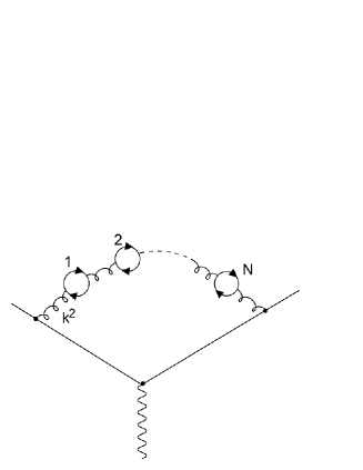
In loop integration these terms introduce a factorial growth, using Eq. 2.15 and considering we obtain:
with . Performing the Borel transform of the last series one obtains a geometric series,
| (2.36) |
which has poles on the real positive axis:
| (2.37) |
These singularities introduce an ambiguity in the inverse Borel transform:
| (2.38) |
since they lie on the path of integration and lead to non-zero residue contributions of the type:
| (2.39) |
IR and UV renormalons arise as singularities on the real negative and positive axis of the complex plane of the Borel transform, (analogously to instanton poles, this explains the name given by ’t Hooft), and are related to the scale and thus to the Landau pole of the strong coupling. These terms affect the coefficients of the perturbative QCD series and its convergence. It has been shown in several applications of resummed quantities (i.e. applying the technique of resummation of large IR logarithms) renormalons do not affect the final result if one uses an appropriate prescription (e.g. the minimal prescription (MP) formula [81, 82]). Reviews on renormalons exist in the literature, e.g. Refs. [83, 84].
Thus, different growths of the coefficients in different
renormalization schemes can balance the differences in values of
the corresponding scales . However, the growth of
the coefficients is not only due to renormalons, in some cases the
coefficients have inherently fast rising behavior as shown in
Ref. [85].
For further insights, relations among different RS and their associated are discussed in Ref. [8].
2.9 The Renormalization Group Equations
The scale dependence of the coupling can be determined considering that the bare coupling and renormalized couplings, , at different scales are related by:
| (2.40) |
where is the regularization parameter, integrals are carried out in dimensions and the UV divergences are regularized to poles. The are constructed as functions of , such that they cancel all poles. From Eq. 2.40 we can obtain the relation from two different couplings at two different scales:
| (2.41) |
with .
The form a group with a composition law:
| (2.42) |
a unity element: and an inversion law: . Fundamental properties of the Renormalization group are:reflexivity, symmetry and transitivity. Thus the scale invariance of a given perturbatively calculated quantity is recovered by the invariance of the theory under the Renormalization Group Equations (RGE). As previously discussed, the QCD Lagrangian has only one dimensionless coupling constant and in the case of a massless theory the Lagrangian has no particular mass scale, but is completely conformal. The only energy scale, , is introduced by the subtraction point with the renormalization procedure. Thus, all phenomena involving strong interactions can be described by only one parameter, the strong coupling , and the same parameter is responsible for the interaction at low and high energy scales. As shown in the previous section, the strong coupling has a running behavior, it evolves and increases with the energy of the probe, , from high to low values of the momentum transfer. Thus if we consider the case of the physical observable at an energy , in order to neglect masses, for example the ratio:
| (2.43) |
where the cross sections are given at the lowest order by:
| (2.44) |
and
| (2.45) |
with the fine structure constant of QED. As shown in the formula the single cross sections depend on the center-of-mass energy , but this dependence cancels in the at lowest order. Also by dimensional analysis, a constant value of the observable would be predicted independently of any energy scale , the ratio being a dimensionless quantity. However, higher order loop integrations and the renormalization procedure of the coupling constant introduce a scale dependence. Since is dimensionless and since there is no mass scale in the QCD Lagrangian, scale dependence can be introduced only via the scale dependence of the coupling and via a ratio -like dependence of the perturbative coefficients. In fact, except for the first two terms which are scale independent, the coefficients are polynomials of with highest power . By means of the RGE all these logarithms can be reabsorbed into the running coupling. The purpose of taking scale-dependent is to transfer to all terms involving in the perturbative series of . The independence of with respect to is given by the Callan-Symanzik relation for QCD [6, 7]:
| (2.46) |
where are quark charges summed over the flavor index and
| (2.47) |
.
| (2.48) |
equivalently:
| (2.49) |
where
| (2.50) |
setting the renormalization scale equal to the physical scale would remove the in the coefficients and fold the -dependence into . Thus the option of choosing yields the simplest form for the perturbative expansions of given observable.
2.10 The Extended Renormalization Group Equations
Given that physical predictions cannot depend on the choice of the renormalization scale nor on the scheme, the same approach used for the renormalization scale based on the invariance under RGE is extended to scheme transformations. This approach leads to the Extended Renormalization Group Equations, which were introduced first by Stückelberg and Peterman [3], then discussed by Stevenson [10, 11, 13, 12] and also improved by Lu and Brodsky [86]. A physical quantity, , calculated at the -th order of accuracy is expressed as a truncated expansion in terms of a coupling constant defined in the scheme and at the scale , such as:
| (2.51) |
At any finite order, the scale and scheme dependencies of the coupling constant and of the coefficient functions do not totally cancel, this leads to a residual dependence in the finite series and to the scale and scheme ambiguities.
In order to generalize the RGE approach it is convenient to improve the notation by introducing the universal coupling function as the extension of an ordinary coupling constant to include the dependence on the scheme parameters
| (2.52) |
where is the standard two-loop scale parameter. The subtraction prescription is now characterized by an infinite set of continuous scheme parameters and by the renormalization scale . Stevenson [11] has shown that one can identify the beta-function coefficients of a given renormalization scheme with the scheme parameters. Considering that the first two coefficients of the -function are scheme independent, each scheme is identified by its parameters.
More conveniently, let us define the rescaled coupling constant and the rescaled scale parameter as
| (2.53) |
Then, the rescaled -function takes the canonical form:
| (2.54) |
with for .
The scheme and scale invariance of a given observable , can be expressed as:
| (2.55) |
The fundamental beta function that appears in Eqs. 2.55 reads:
| (2.56) |
and the extended or scheme-parameter beta functions are defined as:
| (2.57) |
The extended beta functions can be expressed in terms of the fundamental beta function. Since the are independent variables, second partial derivatives respect the commutativity relation:
| (2.58) |
which implies
| (2.59) |
| (2.60) |
where and . From here
| (2.61) |
| (2.62) |
where the lower limit of the integral has been set to satisfy the boundary condition
That is, a change in the scheme parameter can only affect terms of order or higher in the evolution of the universal coupling function.
The extended renormalization group equations Eqs. 2.55 can be written in the form:
| (2.63) |
Thus, provided we know the extended beta functions, we can determine any variation of the expansion coefficients of under scale-scheme transformations. In particular, we can evolve a given perturbative series into another determining the expansion coefficients of the latter and vice versa.
Chapter 3 Renormalization Scale Setting in QCD
The scale-scheme ambiguities are an important source of uncertainties in many processes in perturbative QCD preventing precise theoretical predictions for both SM and BSM physics. In principle, an infinite perturbative series is void of this issue, given the scheme and scale invariance of the entire physical quantities [3, 4, 5, 6, 7], in practice perturbative corrections are known up to a certain order of accuracy and scale invariance is only approximated in truncated series, leading to the scheme and scale ambiguities [8, 9, 10, 11, 12, 13, 14, 15, 16, 17, 87, 88, 18]. If on one hand, according to the conventional practice, or conventional scale setting (CSS), this problem cannot be avoided and is responsible for part of the theoretical errors, on the other hand some strategies for the optimization of the truncated expansion have been proposed, such as the Principle of Minimal Sensitivity proposed by Stevenson [11], the Fastest Apparent Convergence criterion introduced by Grunberg [14] and the Brodsky-Lepage-Mackenzie (BLM) method [17]. These are procedures commonly in use for scale setting in perturbative QCD. In general, a scale-setting procedure is considered reliable if it preserves important self consistency requirements. All Renormalization Group properties such as: uniqueness, reflexivity, symmetry, and transitivity should be preserved also by the scale-setting procedure in order to be generally applied [24].
In fact, once the optimal scale is set, by means of the RG properties is possible to relate results in different schemes and different observables. Other requirements are also suggested by tested theories, by the convergence behavior of the series and also for phenomenological reasons or scheme independence. We discuss in this chapter the different optimization procedures and their properties. An introduction to these methods can also be found in Refs. [21, 22].
3.1 Conventional scale setting - CSS
According to common practice a first evaluation of the physical observable is obtained by calculating perturbative corrections in a given scheme (commonly used are or ) and at an initial renormalization scale , obtaining the truncated expansion:
| (3.1) |
where is the tree-level term, while are the one-loop , two-loop, n-loop corrections respectively and is the power of the coupling at tree-level.
In order to improve the pQCD estimate of the observable, after the initial renormalization a change of scale using the RGE and a chosen scale-setting method is performed in Eq. 3.1, which leads to:
| (3.2) |
where the new leading-order (LO) and higher-order scales and are functions of the initial renormalization scale , and they depend the particular choice of the scale-setting method. At the same time, the new coefficients are changed accordingly in order to obtain a consistent result.
The simple CSS procedure starts from the scale and scheme invariance of a given observable, which translates into complete freedom for the choice of the renormalization scale. In practice in this approach, the initial scale is directly fixed to the typical momentum transfer of the process , , or to a value which minimizes the contributions of the loop diagrams and the errors are evaluated varying the value of in the range of 2, .
It is often claimed that this simple scale setting method estimates contributions from higher-order terms and that, due to the perturbative nature of the expansion, the introduction of higher order corrections would reduce the scheme and scale ambiguities order by order.
No doubt that the higher the loop corrections are calculated, the greater is the precision of the theoretical estimations in comparison with the experimental data, but we cannot know a priori the level of accuracy necessary for the CSS to achieve the desired precision and at present in the majority of cases only the NNLO corrections are available. Besides this, the divergent nature of the asymptotic perturbative series and the presence of factorial growing terms (i.e. renormalons) severely compromise the theoretical predictions.
However, even though this procedure may give an indication on the level of conformality and convergence reached by the truncated expansion, it leads to a numerical evaluation of theoretical errors that is quite unsatisfactory and dependent strictly on the value of the chosen scale. Different choices of the renormalization scale may lead to very different results when including higher order corrections. For example, the NLO correction in W+3jets with the BlackHat code [20] can be either negligible or extremely severe depending on the choice of the particular renormalization scale. One may argue that the proper renormalization scale for a fixed-order prediction can be judged by comparing theoretical results with experimental data, but this method would be strictly process dependent and would compromise the predictivity of the pQCD approach.
Besides the complexity of the higher order calculations and the slow convergence of the perturbative series, there are many critical points in the CSS method:
-
•
In general, no one knows the proper renormalization scale value, , and the correct range where the scale and scheme parameters should be varied in order to have the correct error estimate. In fact, in some processes there can be more than one typical momentum scale that can be taken as the renormalization scale according to the CSS procedure, for example in processes involving heavy quarks, typical scales are either the center-of-mass energy or also the heavy quark mass. Moreover, the idea of the typical momentum transfer as the renormalization scale only sets the order of magnitude of the scale, but does not indicate the optimal scale;
-
•
No distinction is made among different sources of errors and their relative contributions, e.g. in addition to the errors due to scale-scheme uncertainties there are also the errors from missing higher-order uncalculated terms. In such an approach, theoretical uncertainties can become quite arbitrary and unreliable;
-
•
The convergence of the perturbative series in QCD is affected by uncancelled large logarithms as well as by “renormalon” terms that diverge as at higher orders [89, 90], this is known as the renormalon problem [84]. These renormalon terms can give sizable contributions to the theoretical estimates, as shown in annihilation, decay, deep inelastic scattering, hard processes involving heavy quarks. These terms are responsible for important corrections at higher orders also in the perturbative region, leading to different predictions according to different choices of the scale (as shown in Ref. [20]). Large logarithms on the other hand can be resummed using the resummation technique [91, 92, 93, 94, 82, 95, 96] and results are IR renormalon free. This does not help for the renormalization scale and scheme ambiguities, which still affect theoretical predictions with or without resummed large logarithms. In fact, as recently shown in Ref. [2] for the production cross section at NNLO order of accuracy at hadron colliders, the CSS scale setting leads to theoretical uncertainties that are of the same order of the NNLO corrections taking as the typical momentum scale the b-quark mass GeV.
-
•
In the Abelian limit at fixed with , a QCD case approaches effectively the QED analogous case [32, 97]. Thus, in order to be self-consistent any QCD scale-setting method should be also extendable to and results should be in agreement with the Gell-Mann and Low (GM-L) scheme. This is an important requirement also for the perspective of a grand unified theory (GUT), where only one method for setting the renormalization scale can be applied and then it can be considered as a good criterion for verifying if a scale setting is correct or not. CSS leads to incorrect results when applied to QED processes. In the GM-L scheme, the renormalization scale is set with no ambiguity to the virtuality of the exchanged photon/photons, that naturally sums an infinite set of vacuum polarization contributions into the running coupling. Thus the CSS approach of varying the scale of a factor of 2 does not apply to QED since the scale is already optimized.
-
•
The forthcoming large amount of high-precision experimental data arising especially from the running of the high collision energy and high luminosity Large Hadronic Collider (LHC), will require more accurate and refined theoretical estimates. The CSS appears to be more a “lucky guess”; its results are affected by large errors and the perturbative series poorly converges with or without large-logarithm resummation or renormalon contributions. Moreover, within this background, it is nearly impossible to distinguish among SM and BSM signals and in many cases, improved higher-order calculations are not expected to be available in the short term.
To sum up, the conventional scale-setting method assigns an arbitrary range and an arbitrary systematic error to fixed-order perturbative calculations that greatly affects the predictions of pQCD.
3.2 The Principle of Minimal Sensitivity: PMS Scale-Setting
The Principle of Minimal Sensitivity [11, 12] derives from the assumption that, since observables should be independent of the particular RS and scale, their optimal perturbative approximations should be stable under small RS variations. The RS scheme parameters and the scale parameter (or the subtraction point ), are considered as “unphysical” and independent variables, and then their values are set in order to minimize the sensitivity of the estimate to their small variations. This is essentially the core of the Optimized Perturbation Theory (OPT) [11], based on the PMS procedure. The convergence of the perturbative expansion, Eq. 3.1, truncated to a given order , is improved by requiring its independence from the choice of RS and . The optimization is implemented by identifying the RS-dependent parameters in the -truncated series (the for and ), with the request that the partial derivative of the perturbative expansion of the observable with respect to the RS-dependent and scale parameters vanishes. In practice the PMS scale setting is designed to eliminate the remaining renormalization and scheme dependence in the truncated expansions of the perturbative series.
More explicitly, the PMS requires the truncated series, i.e. the approximant of a physical observable defined in Eq. 3.1, to satisfy the RG invariance given by the 2.63, with the substitution of the proper function:
| (3.3) |
it follows that:
| (3.4) | |||||
| (3.5) |
where and . Scheme labels have been omitted. The request of RS-independence modifies the series coefficients and the coupling to the PMS “optimized” values and . At first order the requirement of RS independence implies that Eq. 3.1 satisfies the Callan-Symanzik equation 2.50 with truncated at order . This implies that the scale dependence is not removed from the perturbative coefficients: . We can argue that this approach is more based on convergence rather than physical criteria. In particular, the PMS is a procedure that can be extended to higher order and it can be generally applied to calculations obtained in arbitrary initial renormalization schemes. Though this procedure leads to results that are suggested to be unique and scheme independent, unfortunately it violates important properties of the renormalization group as shown in Ref. [21], such as reflexivity, symmetry, transitivity and also the existence and uniqueness of the optimal PMS renormalization scheme are not guaranteed since they are strictly related to the presence of maxima and minima. Other phenomenological implications will be shown in section 3.5.
3.3 The Fastest Apparent Convergence principle - FAC scale setting
The Fastest Apparent Convergence (FAC) principle is based on the idea of effective charges. As pointed out by Grunberg [14, 15, 16], any perturbatively calculable physical quantity can be used to define an effective coupling, or “effective charge”, by entirely incorporating the radiative corrections into its definition. Effective charges can be defined from an observable starting from the assumption that the infinite series of a given quantity is scheme and scale invariant. Given the perturbative series the relative effective charge is given by
| (3.6) |
Since and are all renormalization scale and scheme invariant, the effective charge is scale and scheme invariant.
The effective charge satisfies the same renormalization group equations as the usual coupling. Thus, the running behavior for both the effective coupling and the usual coupling are the same if their RG equations are calculated in the same renormalization scheme. This idea has been discussed in more detail in Refs. [98, 99].
Using the effective charge , the ratio becomes [100]:
| (3.7) |
where is the Born result and is the center-of-mass energy squared.
An important suggestion is that all effective couplings defined in the same scheme satisfy the same RG equations. While different schemes or effective couplings, will differ through the third and higher coefficients of the -functions, which are scheme dependent. Hence, any effective coupling can be used as a reference to define the renormalization procedure.
Given that expansions of the effective charges are known only up to a certain order, , an optimization procedure is used to improve the perturbative calculations, namely the FAC scale setting. The basic idea of the FAC scale setting method is to set to zero all the higher order perturbative coefficients, i.e. , including all fixed order corrections into the FAC renormalization scale of the leading term by means of the RG equations in order to provide a reliable estimate [101].
In practice given a physical observable in an arbitrary renormalization scheme written as:
the effective coupling is defined by the identity
where and are general perturbative or non-perturbative quantities predicted in principle by QCD, is the -order at the Born level and is the NLO coefficient. Consequently, is the object effectively extracted from a LO analysis of the experimental data on .
In general this method can be applied to any observable calculated in any RS also in processes with large higher order corrections. The FAC scale setting, as has been shown in Ref. [21], preserves the RG self-consistency requirements, although the FAC method can be considered more an optimization approach rather than a proper scale-setting procedure to extend order by order. FAC results depend sensitively on the quantity to which the method is applied. In general, when the NLO correction is large, the FAC results to be a resummation of the most important higher order corrections and then a RG improved perturbation theory is achieved. Unfortunately phenomenological studies (see Fig. 3.1) with FAC show that this strategy is acceptable only in a particular range of values of a given variable related to the virtuality of the physical observable.
3.4 The BLM Scale-Setting
The Brodsky-Lepage-Mackenzie (BLM) [17] method was designed to improve the pQCD estimate by absorbing the -terms arising in the perturbative calculation into the running coupling using the RG equations. In the BLM approach and subsequently in its generalization and extension to all orders the Principle of Maximum Conformality (PMC), the BLM/PMC-scales are identified with the running -terms related to UV divergent loops. In order to improve the discussion, we will use the following notation: for the general number of active flavors, for the number of active flavors related to the UV divergent diagrams and for the number of active flavors related to UV finite diagrams. We underline that only terms related to the -function, or equivalently to , must be included into the BLM/PMC scales. The terms may arise in a calculation but are not responsible for the running of the effective coupling and thus they do not determine the BLM/PMC scales.
The BLM shows a way to resolve the renormalization scheme-scale ambiguities, by identifying the coefficients of the terms. Once these coefficients are reabsorbed into the scale the perturbative expansion no longer suffers of the renormalon growth associated with the , which are eliminated. This improves the convergence of the perturbative expansions in QED/QCD. More importantly, the renormalization scale can be determined without computing all higher-order corrections and in a unambiguous way. Thus, the lower-order or even the LO analysis can be meaningfully compared with experiments. BLM scale setting is greatly inspired by QED. The standard Gell-Mann-Low scheme determines the correct renormalization scale identifying the scale with the virtuality of the exchanged photon [4]. For example, in electron-muon elastic scattering, the renormalization scale is given by the virtuality of the exchanged photon, i.e. the spacelike momentum transfer squared . Thus
| (3.8) |
where
is the vacuum polarization (VP) function. From Eq. 3.8 it follows that the renormalization scale can be determined by the -term at the lowest order. This scale is sufficient to sum all the vacuum polarization contributions into the dressed photon propagator, both proper and improper to all orders.
Following the GM-L scheme in QED, the BLM scales can be determined at LO order in perturbation theory by writing explicit contributions coming from the different terms of the NLO coefficient in a physical observable as [17]:
| (3.9) | |||||
where stands for an initial renormalization scale, which practically can be taken as the typical momentum transfer of the process. The term is due to the quark vacuum polarization. Calculations are in the -scheme.
At the NLO level, all terms should be resummed into the coupling. Using the NLO -running formula:
| (3.10) |
we obtain
| (3.11) |
where
is the BLM scale and
is the conformal coefficient, i.e. the NLO coefficient not depending on the RS and scale . Both the effective BLM scale and the coefficient are independent and conformal at LO. By including the term into the scale we eliminate the term of the NLO coefficient which is responsible for the running of the coupling constant, and the observable in the final results can be written in its maximal conformal form. Eq.3.11.
The BLM method can be extended to higher orders in a systematic way by including the terms arising at higher order into the BLM scales consistently. In order to extend the BLM beyond the NLO, the following points are considered essential:
-
1.
All -terms associated with the -function (i.e. terms) and then with the renormalization of the coupling constant, must be absorbed into the effective coupling, while those -terms that have no relation with UV divergent diagrams (i.e. -terms) should be identified and considered as part of the conformal coefficients. After BLM scale setting, the perturbative series for the physical observable becomes a conformal series, all non-conformal terms should be absorbed into the effective coupling in a consistent manner;
-
2.
New -terms (corresponding to new coefficients) arise at each perturbative order, thus a new BLM scale that sums these terms consistently into the running coupling, should be introduced at each calculated perturbative order. In fact there is no reason to use a unified effective scale for the whole perturbative series as shown in Refs. [102, 103].
-
3.
The BLM scales themselves should be a RG-improved perturbative series [26]. The length of the perturbative series for each BLM scale depends on how many new -terms (or -terms) we have from the higher-order calculation and to what perturbative order we have performed.
Actually the last point is not mandatory and needs clarification. In order to apply the BLM/PMC using perturbative scales, the argument of the coupling in the expansion of the BLM/PMC scale should be the physical scale of the process , that can be either the center-of-mass energy or also another variable such as depending on the process. Setting the initial scale to the physical scale would greatly simplify the BLM/PMC procedure, preserving the original scale invariance of the observable and eliminating the initial scale dependence from the BLM/PMC scales. In case the BLM/PMC scales are not perturbatively calculated, as it will be shown in section 5.1, the initial scale can be treated as an arbitrary parameter.
In agreement with these indications, it is possible to achieve a scale setting method extendible iteratively to all orders, which leads to the correct coefficients for the final “maximally conformal” series:
| (3.12) |
where the BLM scales are set by a recursive use of the RG equations in order to cancel all the terms from the series. We remark that since the coefficients have been obtained cancelling all terms related to running of the coupling they actually are free from any scale and scheme dependence left. In other words the where the are conformal coefficients not depending on the renormalization scale. Hence the BLM approach leads to an observable maximally conformal, i.e. where all the renormalization scale and scheme dependence has been confined to the effective coupling and to its renormalization scale .
Fundamental features of the BLM method:
-
A)
BLM scales at LO , are set simply by identifying the coefficient of the term;
-
B)
since all -terms related to the running of the coupling are reabsorbed, scheme differences do not affect the results and the perturbative expansions in in two different schemes, e.g. and , are identical. We notice that -terms related to the UV finite diagrams, may arise at every order in perturbation theory. These terms might be related either to the particular kinematics of the initial state or even to finite loop diagrams arising at higher orders, thus in both cases are insensitive to the UV cutoff or to the RS and cannot be considered as -terms. We label these terms as -terms and they do not give contributions to the BLM scales;
-
C)
Using BLM scale setting, the perturbative expansion does not change across quark threshold, given that all vacuum-polarization effects due to a new quark are automatically absorbed into the effective coupling. This implies that in a process with fixed kinematic variables (e.g. a total cross section), we can use a naive LO/NLO -running with the number of active flavor fixed to the value determined by the BLM scale, to perform the calculation [104];
-
D)
The BLM method preserves all the RG properties of existence and uniqueness, reflexivity, symmetry, and transitivity. As shown in Refs. [105, 106, 107, 108], the RG invariance of the BLM leads to scheme independent transformations that relate couplings in different schemes. These are known as commensurate scale relations (CSRs), and it has been shown that even though the expansion coefficients under different renormalization schemes can be different, after a proper scale setting, one can determine a relation between the effective couplings leading to an invariant result for the calculated quantity. Using this approach it is also possible to extend conformal properties to renormalizable gauge theories, such as the generalized Crewther relation [109, 110, 111, 112];
-
E)
The BLM approach reduces to the GM-L scheme for QED in the Abelian limit [32], the results are in perfect agreement;
-
F)
The elimination of the term related with the coefficient, from the perturbative series eliminates the renormalon terms over the entire range of the accessible physical energies and not only in the low-energy domain. The convergence of the resulting series is then greatly improved.
3.5 Phenomenological comparison
Though results should be invariant with respect to the particular method used for scale-setting, at a low level of accuracy (NLO,NNLO,..) they can be different and even incorrect or unphysical. Since the scale setting methods, such as FAC, PMS and BLM/PMC, are designed from different fundamental principles, they can give strikingly different results in practical applications. In fact, as shown by Kramer and Lampe [23], the resulting PMS and FAC scales can be unphysical, Fig.3.1;this is the case of the prediction of jet production fractions in annihilation, the PMS and the FAC scale grow without bound when the gluon virtuality becomes soft.
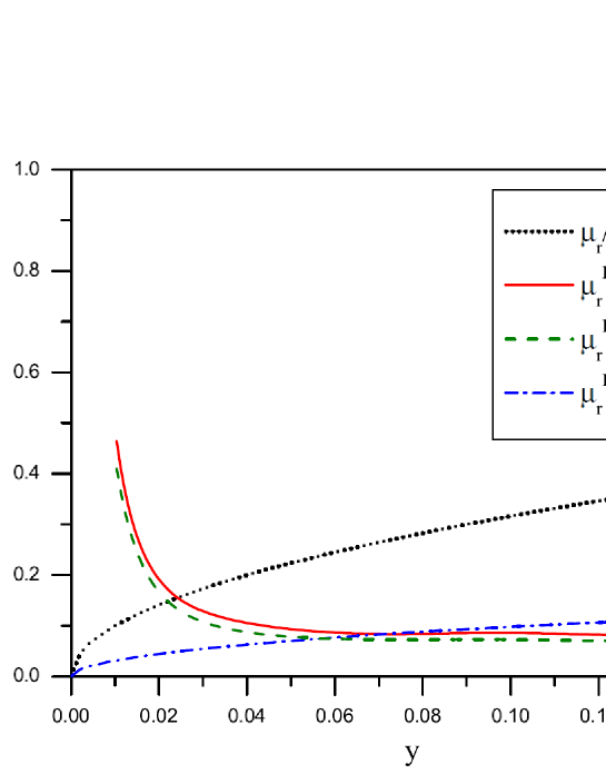
Usually, jets are defined by clustering particles in narrow cones with invariant mass less than , where stands for the resolution parameter and is the total center-of-mass energy. Physically, one expects the renormalization scale to reflect the invariant mass of the jet. For example, in the analogous problem in QED, the maximum virtuality of the photon jet which sets the argument of the running coupling cannot be larger than . Thus one expects to decrease as . However, as shown in the Fig. 3.1, the scales chosen by the FAC and PMS methods do not reproduce this physical behavior: The predicted scales and rise at small values of the invariant mass . This shows that the FAC and PMS cannot get the right physical behavior in this limit, since they have included also physics into the running coupling not associated with renormalization. On the other hand, the BLM/PMC scale has the correct physical behavior approaching low values, , which indicates the breaking of standard pQCD [113], while in contrast, the scales chosen by PMS and FAC show no indications of non-perturbative effects.
Chapter 4 The Principle of Maximum Conformality - PMC scale setting
The Principle of Maximum Conformality (PMC) [25, 26, 27, 28, 29] is the principle underlying BLM and it generalizes the BLM method to all possible applications and to all orders.
Several extended versions of the BLM approach beyond the NLO have been proposed in the literature such as the dressed skeleton expansion, the large -expansion, the BLM expansion with an overall renormalization scale, the sequential BLM (seBLM), an extension to the sequential BLM (xBLM) in Refs. [114, 115, 108, 112, 102, 116, 117, 118]. These different extensions of the BLM are mostly partial or ad hoc improvements of the first LO-BLM [17] in some cases up to NNLO, in other cases using a rather effective approach, i.e. by introducing an overall effective BLM scale for the entire perturbative expansion. Results obtained with these approaches did not respect also the basic points (1-3) explained in section 3.4. Most important, these methods lead to results that are still dependent on the initial renormalization scale. The fundamental feature of the BLM is to obtain results free from scale ambiguities and thus independent of the choice of initial renormalization scale. The first aim of the BLM scale is to eliminate the renormalization scale and scheme uncertainties; thus any extension of the BLM not respecting this basic requirement does not represent a real improvement of the standard conventional scale setting CSS method.
The reasons for the different extensions of the BLM method to higher order were mainly two: first it was not clear how to generalize this approach to all possible quantities, which translates into the question: what is the principle underlying the BLM method? And second, what is the correct procedure to identify and reabsorb the -terms unambiguously order-by-order? A practical reason that makes the extension to higher orders not straightforward is the presence of UV finite corrections given by the three and four-gluon vertices of the additional -terms that are unrelated to the running of .
In its first formulation in Ref. [25] it was suggested to use a unique scale at LO to reabsorb all contributions related to different skeleton graphs scale by properly weighting the two contributions, such as that of the t-channel and s-channel. This approach was more oriented towards a single PMC scale that reabsorbs all terms related to the running coupling. A multi-scale approach was later developed considering different scales arising at each order of accuracy including different coefficients according to the perturbative expansion. We remark that the PMC method has all the (A,B,C,D,E,F) properties of the BLM procedure (Sec. 3.4) and it extends these properties to all orders eliminating the renormalization scale and scheme ambiguities. The PMC also generalizes this approach to all gauge theories. First this is crucial in order to apply the same method to all SM sectors. Secondly, in the perspective of a grand unified theory (GUT), only one scale setting method can be applied for consistency, and this method must agree with the GM-L scheme and with the QED results.
In order to apply the PMC is convenient to follow the flowchart shown in Fig. 4.1 and to write the observable of Eq. 3.1 with the explicit contributions of the terms in the coefficients calculated at each order of accuracy:
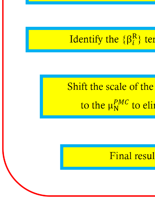
| (4.1) |
where represents the kinematic scale or the physical scale of the measured observable and is the power of associated with the tree-level terms. In general, this procedure is always possible either for analytic or numerical (e.g. MonteCarlo) calculations, given that both strategies keep track of terms related to different color factors. The core of the PMC method, as was for BLM, is that all terms related to the -function arising in a perturbative calculation must be summed, by proper definition of the renormalization scale , into the effective coupling by recursive use of the RGE. Essentially the difference between the two procedures is that while in BLM the scales are set iteratively order by order to remove all terms, in PMC the terms are written first as terms and then reabsorbed into the effective coupling. The two procedures are related by the correspondence principle [26].
4.1 The multi-scale Principle of Maximum Conformality: PMCm
The PMCm method is based on a multi-scale application of the PMC. We show in this section how to implement this method at any order of accuracy. First, as shown in the flowchart in Fig. 4.1, for the pQCD approximant (4.1), it is convenient to transform the series at each order into the series. The QCD degeneracy relations [119] ensure the realizability of such transformation. For example, Eq. 4.1 can be rewritten as [28, 29]
| (4.2) | |||||
where can be derived from ; are conformal coefficients, and are nonconformal. For definiteness and without loss of generality, we have set and for illustrating the PMC procedures. Different types of -terms can be absorbed into in an order-by-order manner by using the RGE, which leads to distinct PMC scales at each order:
| (4.3) | |||||
The coefficients are generally functions of , which can be redefined as
| (4.4) |
where the reduced coefficients (specifically, we have ), and the combinatorial coefficients . As discussed in section 3.4, we set the renormalization scale to the physical scale of the process :
| (4.5) | |||||
| (4.6) | |||||
| (4.7) |
Note that the PMC scales are of a perturbative nature, which is also a kind of resummation and we need to know more loop terms to achieve more accurate predictions. The PMC resums all the known same type of -terms to form precise PMC scales for each order. Thus, the precision of the PMC scale for the high-order terms decreases at the higher-and-higher orders due to the less known -terms in those higher-order terms. For example, is determined up to next-to-next-to-leading log (N2LL)-accuracy, is determined up to NLL-accuracy and is determined at the LL-accuracy. Thus the PMC scales at higher-orders are of less accuracy due to more of its perturbative terms being unknown. This perturbative property of the PMC scale causes the first kind of residual scale dependence.
After fixing the magnitude of , we achieve a conformal series
| (4.8) |
The PMC scale for the highest-order term, e.g. for the present case, is unfixed, since there is no -terms to determine its magnitude. This renders the last perturbative term unfixed and causes the second kind of residual scale dependence. Usually, the PMCm suggests setting as the last determined scale , which ensures the scheme independence of the prediction due to commensurate scale relations among the predictions under different renormalization schemes [108, 120]. The pQCD series (4.8) is renormalization scheme and scale independent, and becomes more convergent due to the elimination of the terms including those related to the renormalon divergence. Thus a more accurate pQCD prediction can be achieved by applying the PMCm. Two residual scale dependences are due to perturbative nature of either the pQCD approximant or the PMC scale, which is in principal different from the conventional arbitrary scale dependence. In practice, we have found that those two residual scale dependences are quite small even at low orders. This is due to a generally faster pQCD convergence after applying the PMCm. Some examples can be found in Ref. [121].
4.2 The single-scale Principle of Maximum Conformality: PMCs
In some cases, the perturbative series might have a weak convergence and the PMC scales might retain a comparatively larger residual scale dependence. In order to overcome this a single scale approach has been proposed, namely the PMCs, in order to suppress the residual scale dependence by directly fixing a single effective . Following the standard procedures of PMCs [122], the pQCD approximant (4.2) changes to the following conformal series,
| (4.9) |
As in the previous section, we have set and for illustrating the procedure. The PMC scale can be determined by requiring all the nonconformal terms vanish, which can be fixed up to N2LL-accuracy for and , i.e. can be expanded as a power series over ,
| (4.10) |
where the coefficients are
| (4.11) | |||||
| (4.12) |
and
| (4.13) | |||||
Eq. 4.10 shows that the PMC scale is also a power series over , which resums all the known -terms and is explicitly independent of at any fixed order, but depends only on the physical scale Q. It represents the correct momentum flow of the process, and determines an overall effective value. Together with the -independent conformal coefficients, the resultant PMC pQCD series is scheme and scale independent [123]. By using a single PMC scale determined with the highest accuracy from the known pQCD series, both the first and the second kind of residual scale dependence are suppressed.
Chapter 5 Infinite-Order Scale-Setting using the Principle of Maximum Conformality: PMC∞
We introduce in this chapter a parametrization of the observables that stems directly from the analysis of the perturbative QCD corrections and which reveals interesting properties like scale invariance independently of the process or of the kinematics. We point out that this parametrization can be an intrinsic general property of gauge theories and we define this property as intrinsic conformality (iCF111Here the conformality has to be understood as RG invariance only.). We also show how this property directly indicates the correct renormalization scale at each order of calculation and we define this new method PMC∞: Infinite-Order Scale-Setting using the Principle of Maximum Conformality. We apply the iCF property and the PMC∞ to the case of the thrust and C-parameter distributions in and we show the results.
5.1 Intrinsic conformality (iCF)
In order to introduce intrinsic conformality (iCF), we consider the case of a normalized IR-safe single-variable distribution and write the explicit sum of pQCD contributions calculated up to NNLO at the initial renormalization scale :
| (5.1) | |||||
where the is tree-level hadronic cross section, the are respectively the LO, NLO and NNLO coefficients, is the selected non-integrated variable. For the sake of simplicity we will refer to the perturbatively calculated differential coefficients as implicit coefficients and we drop the derivative symbol, i.e.
| (5.2) |
We define here the intrinsic conformality as the property of a renormalizable SU(N)/U(1) gauge theory, like QCD, which yields a particular structure of the perturbative corrections that can be made explicit representing the perturbative coefficients using the following parametrization222We are neglecting here other running parameters such as the mass terms.:
where the are the scale invariant Conformal Coefficients (i.e. the coefficients of each perturbative order not depending on the scale ) while we define the as Intrinsic Conformal Scales and are the first two coefficients of the -function. We recall that the implicit coefficients are defined at the scale and that they change according to the standard RG equations under a change of the renormalization scale according to :
It can be shown that the form of Eq. LABEL:newevolution is scale invariant and it is preserved under a change of the renormalization scale from to by standard RG equations Eq. LABEL:standardevolution, i.e.:
| (5.5) | |||||
We note that the form of Eq. LABEL:newevolution is invariant and that the initial scale dependence is exactly removed by . Extending this parametrization to all orders we achieve a scale invariant quantity: the iCF-parametrization is a sufficient condition in order to obtain a scale invariant observable.
In order to show this property we collect together the terms identified by the same conformal coefficient, we name each set as a conformal subset and we extend the property to order :
| (5.6) | |||||
in each subset we have only one intrinsic scale and only one conformal coefficient and the subsets are disjoint; thus no mixing terms among the scales or the coefficients are introduced in this parametrization. Moreover, the structure of the subsets remains invariant under a global change of the renormalization scale, as shown from Eq. 5.5. The structure of each conformal set and consequently the iCF are preserved also if we fix a different renormalization scale for each conformal subset, i.e.
| (5.7) |
We define here this property of Eq. 5.6 of separating an observable in the union of ordered scale invariant disjoint subsets an ordered scale invariance.
In order to extend the iCF to all orders, we perform the limit using the following strategy: we first perform a partial limit including the higher order corrections relative only to those terms that have been determined already at order for each subset, and then we perform the complementary limit, which consists in including all the remaining higher order terms. For the limit we have:
| (5.8) |
where is the coupling calculated up to at the intrinsic scale . Given the particular ordering of the powers of the coupling, in each conformal subset we have the coefficients of the terms, where is the order of the conformal subset and the is the order of the highest subset with no -terms. We note that the limit of each conformal subset is finite and scale invariant up to . The remaining scale dependence is confined in the coupling of the term. Any combination of the subsets is finite and scale invariant. We can now extend the iCF to all orders performing the limit. In this limit we include all the remaining higher order corrections. For the calculated conformal subsets this leads to define the coupling at the same scales but including all the missing terms. Thus each conformal subset remains scale invariant. We point out that we are not making any assumption on the convergence of the series for this limit. Thus, we have:
where here now is the complete coupling determined at the same scale . Eq. LABEL:nlimit shows that the whole renormalization scale dependence has been completely removed. In fact, neither the intrinsic scales nor the conformal coefficients depend on the particular choice of the initial scale. The only term with a residual dependence is the n-term, but this dependence cancels in the limit . The scale dependence is totally confined to the coupling and its behavior does not depend on the particular choice of any scale in the perturbative region, i.e. with . Hence the limit of depends only on the properties of the theory and not on the scale of the coupling in the perturbative regime. The proof given here shows that the iCF is sufficient to have a scale invariant observable and it does not depend on the particular convergence of the series. In order to show the necessary condition we separate the two cases of a convergent series and an asymptotic expansion. For the first case the necessary condition stems directly from the uniqueness of the iCF form, since given a finite limit and the scale invariance any other parametrization can be reduced to the iCF by means of appropriate transformations in agreement with the RG equations. For the second case, we have that an asymptotic expansion though not convergent, can be truncated at a certain order , which is the case of Eq. 5.6. Given the particular structure of the iCF we can perform the first partial limit and we would achieve a finite and scale invariant prediction , , for a truncated asymptotic expansion, as shown in Eq. 5.8. Given the truncation of the series in the region of maximum of convergence the n-th term would be reduced to the lowest value and so the scale dependence of the observable would reach its minimum. Given the finite and scale invariant limit we conclude that the iCF is unique and thus necessary for an ordered scale invariant truncated asymptotic expansion up to the order. We point out that in general the iCF form is the most general and irreducible parametrization which leads to the scale invariance, other parametrization are forbidden since if we introduce more scales 333Here we refer to the form of Eq. LABEL:newevolution. In principle it is possible to write other parametrizations preserving the scale invariance, but these can be reduced to the iCF by means of appropriate transformations in agreement with the RG equations. into the logarithms of one subset we would spoil the invariance under the RG transformation and we could not achieve Eq. 5.5, while on the other hand no scale dependence can be introduced into the intrinsic scales since it would remain in the observable already in the first partial limit and it could not be eliminated. The conformal coefficients are conformal by definition at each order, thus they do not depend on the renormalization scale and they do not have a perturbative expansion. Hence the iCF is a necessary and sufficient condition for scale invariance.
5.2 Comments on the iCF and the ordered scale invariance
The iCF-parametrization can stem either from an inner property of the theory, the iCF, or from direct parametrization of the scale-invariant observable. In both cases the iCF-parametrization makes the scale dependence of the observable explicit and it exactly preserves the scale invariance. The iCF parametrization is invariant with respect to the choice of initial scale , this implies that the same calculation performed choosing different arbitrary initial scales, leads to the same result in the limit , a limit that is scale and scheme independent. The iCF is also strongly motivated by the renormalizability of QCD and by the uniqueness of the function in a given scheme, i.e. two different do not occur in a perturbative calculation at any order in one RS and the UV divergencies are cancelled by redefinition of the same parameters at lowest and higher orders. We remark that the conservation of the iCF form in one observable is strongly related to the validity of the RG transformations, thus we expect the iCF to be well preserved in the deep Euclidean region.
Once we have defined an observable in the iCF-form, we have not only the scale invariance of the entire observable, but also the ordered scale invariance (i.e. the scale invariance of each subset or ). The latter property is crucial in order to obtain scale invariant observables independently from the particular kinematic region and independently from the starting order of the observable or the order of the truncation of the series. Since in general, a theory is blind with respect to the particular observable/process that we might investigate, the theory should preserve the ordered scale invariance in order to define always scale invariant observables. Hence if the iCF is an inner property of the theory, it leads to implicit coefficients that are neither independent nor conformal. This is made explicit in Eq. LABEL:newevolution, but it is hidden in the perturbative calculations in the case of the implicit coefficients. For instance, the presence of the iCF clearly reveals itself when a particular kinematic region is approached and the becomes null. This would cause a breaking of the scale invariance since a residual initial scale dependence would remain in the observable in the higher order coefficients. The presence of the iCF solves this issue by leading to the correct redefinition of all the coefficients at each order preserving the correct scale invariance exactly. Thus, in the case of a scale-invariant observable , defined according to the implicit form (Eq. 5.1), by the coefficients it cannot simply undergo the change , since this would break the scale invariance. In order to preserve the scale invariance, we must redefine the coefficients cancelling out all the initial scale dependence originating from the LO coefficient at all orders. This is equivalent to subtracting out a whole invariant conformal subset related to the coefficient from the scale invariant observable . This mechanism is clear in the case of the explicit form of the iCF, Eq. LABEL:newevolution, where if then the whole conformal subset is null and the scale invariance is preserved. We underline that the conformal coefficients can acquire all possible values without breaking the scale invariance, they contain the essential information on the physics of the process, while all the correlation factors can be reabsorbed into the renormalization scales as shown by the PMC method [26, 26, 27, 28, 29]. Hence if a theory has the property of ordered scale invariance, it preserves exactly the scale invariance of observables independently of the process, the kinematics and the starting order of the observable. We underline that if a theory has the intrinsic conformality all the renormalized quantities, such as cross sections, can be parametrized with the iCF-form. This property should be preserved by the renormalization scheme or by the definition of IR safe quantities and it should be preserved also in observables defined in effective theories. The iCF shows that point (3) of the BLM/PMC approach (Section 3.4) can be improved by eliminating the perturbative expansion of the BLM/PMC scales, leading to a scale and scheme invariant result. Though we remark that the perturbative corrections in the BLM or PMCm scales are suppressed in the perturbative region.
5.3 The PMC∞
We introduce here a new method to eliminate the scale-setting ambiguity in single variable scale invariant distributions, which we call PMC∞. This method is based on the original PMC principle and agrees with all the different PMC formulations for the PMC-scales at the lowest order. Essentially the core of the PMC∞ is the same for all the BLM-PMC prescriptions, i.e. the effective running coupling value and hence its renormalization scale at each order is determined by the -term of the next higher order, or equivalently by the intrinsic conformal scale . The PMC∞ preserves the iCF and thus the scale and scheme invariance, absorbing an infinite set of -terms to all orders. This method differs from the other PMC prescriptions since, due to the presence of the intrinsic conformality, no perturbative correction in needs to be introduced at higher orders in the PMC-scales. Given that all the -terms of a single conformal subset are included in the renormalization scale already with the definition at lowest order, no initial scale or scheme dependence are left due to the unknown -terms in each subset. The PMC∞-scale of each subset can be unambiguously determined by -term of each order, we underline that all logarithms of each subset have the same argument and all the differences arising at higher orders have to be included only in the conformal coefficients. Reabsorbing all the -terms into the scale also the terms (related to renormalons [84]) are eliminated, thus the precision is improved and the perturbative QCD predictions can be extended to a wider range of values. The initial scale dependence is totally confined in the unknown PMC∞ scale of the last order of accuracy (i.e. up to NNLO case in the ). Thus if we fix the renormalization scale independently to the proper intrinsic scale for each subset , we end up with a perturbative sum of totally conformal contributions up to the order of accuracy:
| (5.10) | |||||
at this order, the last scale is set to the physical scale Q, i.e. .
5.4 iCF coefficients and scales: a new “How-To” method
We describe here how all the coefficients of Eq. LABEL:newevolution can be identified from either a numerical or analytical perturbative calculation. This method applies in general to any perturbative calculation once results for the different color factors are kept separate, however we refer to the particular case of the NNLO thrust distribution results calculated in Refs. [124, 125] for the purpose. Since the leading order is already () void of -terms we start with NLO coefficients. A general numerical/analytical calculation keeps tracks of all the color factors and the respective coefficients:
| (5.11) |
where , and The dependence on is made explicit here for sake of clarity. We can determine the conformal coefficient of the NLO order straightforwardly, by fixing the number of flavors in order to kill the term:
| (5.12) |
we would achieve the same results in the usual PMC way, i.e. identifying the coefficient with the term and then determining the conformal coefficient. Both methods are consistent and results for the intrinsic scales and the coefficients are in perfect agreement. At the NNLO a general coefficient is composed of the contribution of six different color factors:
| (5.13) | |||||
In order to identify all the terms of Eq. LABEL:newevolution we notice first that the coefficients of the terms and are already given by the NLO coefficient , thus we need to determine only the and the conformal terms. In order to determine the latter coefficients we use the same procedure we used for the NLO; i.e. we set the number of flavors in order to drop off all the terms. We have then:
with . This procedure can be extended to every order and one may decide whether to cancel , or by fixing the appropriate number of flavors. The results can be compared leading to determine exactly all the coefficients. We point out that extending the intrinsic conformality to all orders we can predict at this stage the coefficients of all the color factors of the higher orders related to the -terms except those related to the higher order conformal coefficients and -terms (e.g. at NNNLO the and ). The -terms are coefficients that stem from UV-divergent diagrams connected with the running of the coupling constant and not from UV-finite diagrams. UV-finite terms may arise but would not contribute to the -terms. These terms can be easily identified by the kinematic constraint at lowest order or by checking deviations of the coefficients from the iCF form. In fact, only the terms coming from UV-divergent diagrams, depending dynamically on the virtuality of the underlying quark and gluon subprocesses have to be considered as -terms and they would determine the intrinsic conformal scales. In general, each is an independent function of the physical scale of the process (or ), of the selected variable and it varies with the number of colors mainly due to and vertices. The latter terms arise at higher orders only in a non-Abelian theory but they are not expected to spoil the iCF-form. We underline that iCF applies to scale-invariant single-variable distributions, in case one is interested in the renormalization of a particular diagram, e.g. the vertex, contributions from different -terms should be singled out in order to identify the respective intrinsic conformal scale consistently with the renormalization of the non-Abelian vertex, as shown in [126].
5.5 PMC∞ results for thrust and C-parameter
The thrust distribution and the event shape variables are a
fundamental tool in order to probe the geometrical structure of a
given process at colliders. Being observables that are exclusive
enough with respect to the final state, they allow for a deeper
geometrical analysis of the process and they are also particularly
suitable for the measurement of the strong coupling [127].
Given the high precision data collected at LEP and
SLAC [128, 129, 130, 131, 132],
refined calculations are crucial in order to extract information
to the highest possible precision. Though extensive studies on
these observables have been released during the last decades
including higher order corrections from next-to-leading order
(NLO) calculations [133, 134, 135, 136, 137, 138]
to the next-to-next-to-leading
order(NNLO) [139, 140, 141, 124, 125] and
including resummation of the large logarithms [96, 95], the theoretical predictions are still affected by
significant theoretical uncertainties that are related to large
renormalization scale ambiguities.
In the particular case of the three-jet event-shape distributions the conventional practice of CSS leads to results that do not match the experimental data and the extracted values of deviate from the world average [34].
The thrust () and C-parameter () are defined as
| (5.15) |
| (5.16) |
where the sum runs over all particles in the hadronic final state, and denotes the three-momentum of particle . The unit vector is varied to maximize thrust , and the corresponding is called the thrust axis and denoted by . The variable is often used, which for the LO of 3-jet production is restricted to the range . We have a back-to-back or a spherically symmetric event respectively at and at respectively. For the C-parameter, is the angle between and . At LO for the 3 jet production the C-parameter is restricted to the range: by kinematics.
In general a normalized IR-safe single-variable observable, such as the thrust distribution for the [142, 143], is the sum of pQCD contributions calculated up to NNLO at the initial renormalization scale :
| (5.17) | |||||
where , is the selected
event shape variable, the cross section of the process,
is the total hadronic cross section and are respectively the normalized LO, NLO and NNLO coefficients:
| (5.18) | |||||
where are the coefficients normalized to the tree-level cross section calculated by MonteCarlo (see e.g. the EERAD and Event2 codes [139, 140, 141, 124, 125]) and are:
| (5.19) |
where is the Riemann zeta function.
In general according to CSS the renormalization scale is set to and theoretical uncertainties are evaluated using standard criteria. In this case, we have used the definition given in Ref. [140] of the parameter , we define the average error for the event shape variable distributions as:
| (5.20) |
where is the index of the bin and is the total number of bins, the renormalization scale is varied in the range: .
5.6 The PMC∞ scales at LO and NLO
According to the PMC∞ prescription we fix the renormalization scale to at each order absorbing all the terms into the coupling. We notice a small mismatch between the zeroes of the conformal coefficient and those of the remaining term in the numerator (the formula is shown in Eq. LABEL:Cconf). Due to our limited knowledge of the strong coupling at low energies, in order to avoid singularities in the NLO-scale , we introduce a regularization that leads to a finite scale in the whole range of values of the variable . These singularities might be due either to the presence of UV finite terms or to the logarithmic behavior of the conformal coefficients when low values of the variable are approached. Large logarithms arise from the IR-divergence cancellation procedure and they can be resummed in order to restore a predictive perturbative regime [91, 92, 93, 94, 144, 95, 96]. We point out that IR cancellation should not spoil the iCF property. Whether this is an actual deviation from the iCF-form has to be further investigated. However, since the discrepancies between the coefficients are rather small, we introduce a regularization method based on redefinition of the norm of the coefficient in order to cancel out these singularities in the -scale. This regularization is consistent with the PMC principle and up to the accuracy of the calculation it does not introduce any bias effect in the results or any ambiguity in the NLO-PMC∞ scale. All the differences introduced by the regularization would start at the order of accuracy and they can be reabsorbed after in the higher order PMC∞ scales. Thus we obtain for the PMC∞ scales, :
| (5.21) | |||||
| (5.26) |
where and the third scale is set to . The renormalization scheme factor for the QCD results is set to . This scheme factor reabsorbs also the scheme difference into the renormalization scale and is related to the particular choice of the scale parameter as discussed in section 2.8. The coefficients are the coefficients related to the -terms of the NLO and NNLO perturbative order of the thrust distribution respectively. They are determined from the calculated coefficients.
The parameter is a regularization term to cancel the singularities of the NLO scale, , in the range , depending on non-matching zeroes between numerator and denominator in the . In general this term is not mandatory for applying the PMC∞, it is necessary only in case one is interested in applying the method all over the entire range covered by the thrust, or any other observable. Its value has been determined as for the thrust distribution and it introduces no bias effects up to the accuracy of the calculations and the related errors are totally negligible up to this stage.
We point out that in the region we have a clear example of intrinsic conformality-iCF where the kinematic constraints set the . According to Eq. 5.5 setting the the whole conformal subset becomes null. In this case all the terms at NLO and NNLO disappear except the -term at NNLO which determines the scale. The surviving terms at NLO or the at NNLO are related to the finite -term at NLO and to the mixed term arising from at NNLO. Using the parametrization with explicit terms we have for :
| (5.27) |
we can determine the for the region as shown in Eq. 5.26:
| (5.28) |
by identifying the -term at NNLO. The LO and NLO PMC∞ scales are shown in Fig. 5.1.
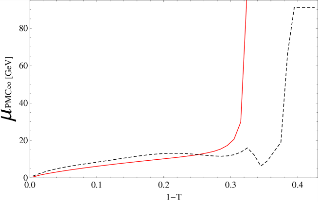
We notice that the two PMC∞ scale have similar behaviors in the range and the LO-PMC∞ scale agrees with the PMC scale used in Ref. [146]. This method totally eliminates both the ambiguity in the choice of the renormalization scale and the scheme dependence at all orders in QCD.
5.7 NNLO Thrust distribution results
We use here the results of Ref. [124, 125] and for the running coupling we use the RunDec program [147]. In order to normalize consistently the thrust distribution we expand the denominator in while the numerator has the couplings renormalized at different PMC∞ scales , . We point out here that the proper normalization would be given by the integration of the total cross section after renormalization with the PMC∞ scales, nonetheless since the PMC∞ prescription involves only absorption of higher order terms into the scales, the difference would be within the accuracy of the calculations, i.e. . Eq. 5.17 becomes:
| (5.29) |
where the are normalized subsets that are given by:
are the scale-invariant conformal coefficients (i.e. the coefficients of each perturbative order not depending on the scale ) while are the couplings determined at the scales respectively.
Normalized subsets for the region can be achieved simply by setting in the Eq. LABEL:normalizedcoeff. Within the numerical precision of these calculations there is no evidence of the presence of spurious terms, such as any further UV-finite term up to NNLO [148] besides the kinematic term at lowest order in the multi-jet region. These terms, if there are any, must remain rather small all over the range of the thrust variable in comparison with the term or even be compatible with numerical fluctuations. Moreover, we notice a small rather constant difference between the iCF-predicted and the calculated coefficient for the -color factor of Ref. [124] which might be due to a UV-finite coefficient or possibly to statistics. This small difference must be included in the conformal coefficient but it has a completely negligible impact on the total thrust distribution.
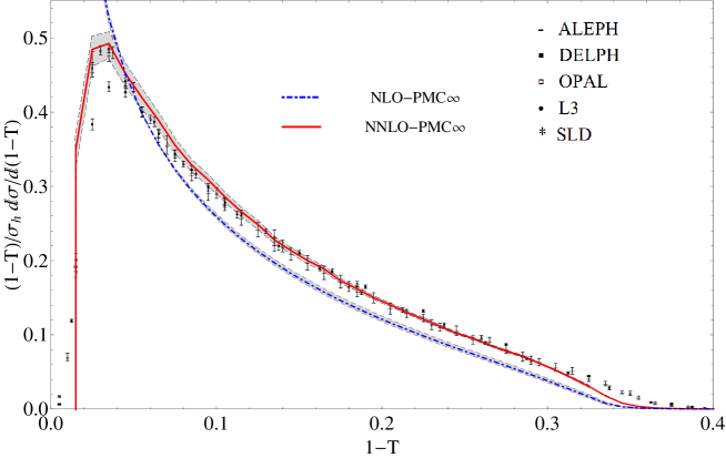
In Fig. 5.2 we show the thrust distribution at NLO and at NNLO with the use of the PMC∞ method. Theoretical errors for the thrust distribution at NLO and at NNLO are also shown (the shaded area). Conformal quantities are not affected by a change of renormalization scale. Thus the errors shown give an evaluation of the level of conformality achieved up to the order of accuracy and they have been calculated using standard criteria, i.e. varying the remaining initial scale value in the range . Using the same definition of the parameter given in Eq. 5.20, we have in the interval an average error of and for the thrust at NLO and at NNLO respectively. A larger improvement has been obtained in the entire range of reliable results for thrust distribution, i.e. , from to from NLO to the NNLO accuracy with the PMC∞.
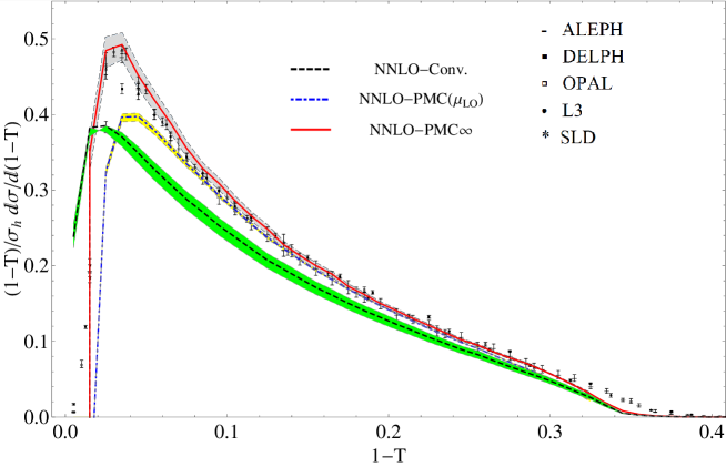
In Fig. 5.3 a direct comparison of the PMC∞ with the CSS results (obtained in [124] and [140, 141]) is shown. In addition, we have shown also the results of the first PMC approach used in [146], which we indicate as PMC(LO) extended to NNLO accuracy. In this approach the last unknown PMC scale NLO of the NLO was set to the last known PMC scale LO of the LO, while the NNLO scale NNLO was left unset and varied in the range . This analysis was performed in order to show that the procedure of setting the last unknown scale to the last known one leads to stable and precise results and is consistent with the proper PMC method in a wide range of values of the variable.
| Conv. | PMC(LO) | PMC∞ | |
|---|---|---|---|
| 6.03 | 1.41 | 1.31 | |
| 6.97 | 2.19 | 0.98 | |
| 8.46 | - | 2.61 | |
| 5.34 | 1.33 | 1.77 | |
| 6.00 | - | 1.95 |
Average errors calculated in different regions of the spectrum are reported in Table 5.1. From the comparison with the CSS we notice that the PMC∞ prescription significantly improves the theoretical predictions. Moreover, results are in remarkable agreement with the experimental data in a wider range of values and they show an improvement of the PMC results when the two-jets and the multi-jets regions are approached, i.e. the region of the peak and the region respectively. The use of the PMC∞ approach in perturbative thrust QCD calculations restores the correct behavior of the thrust distribution in the region and this is a clear effect of the iCF property. Comparison with experimental data has been improved all over the spectrum and the introduction of the order correction would improve this comparison especially in the multi-jet region. In the PMC∞ method theoretical errors are given by the unknown intrinsic conformal scale of the last order of accuracy. We expect this scale not to be significantly different from that of the previous orders. In this particular case, as shown in Eq. LABEL:normalizedcoeff, we have also a dependence on the initial scale left due to the normalization and to the regularization terms. These errors represent 12.5% and 1.5% respectively of the whole theoretical errors in the range and they could be improved by means of a correct normalization.
5.8 NNLO C-parameter distribution results
The same analysis applies straightforwardly to the C-parameter distribution including the regularizing parameter, which has been set to the same value . The same scales of Eq. 5.21 and Eq. 5.26 apply to the C-parameter distribution in the region and in the region . In fact, due to kinematic constraints that set the , we have the same iCF effect also for the C-parameter. Results for the C-parameter scales and distributions are shown in Fig. 5.4 and Fig. 5.5 respectively.
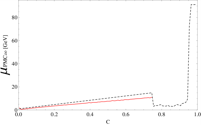
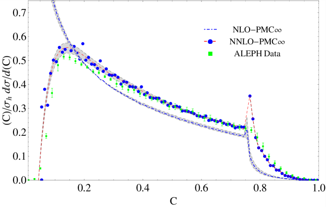
Theoretical errors have been calculated, as in the previous case, using standard criteria and results indicate an average error over the whole spectrum of the C-parameter distribution at NLO and at NNLO of and respectively.
| [%] | Conv. | PMC(LO) | PMC∞ |
|---|---|---|---|
| 4.77 | 0.85 | 2.43 | |
| 11.51 | 3.68 | 2.42 | |
| 6.47 | 1.55 | 2.43 |
A comparison of average errors according to the different methods is shown in Table 5.2. Results show that the PMC∞ improves the NNLO QCD predictions for the C-parameter distribution over the entire spectrum.
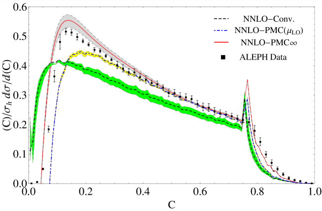
A comparison of the distributions calculated with the CSS, the PMC(LO) [149] and the PMC∞ is shown in Fig. 5.6. Results for the PMC∞ show remarkable agreement with the experimental data away from the regions and . The errors due to the normalization and to the regularization terms (Eq. LABEL:normalizedcoeff) are respectively and of the whole theoretical errors. The perturbative calculations could be further improved using a correct normalization and also by introducing the large-logarithm resummation technique in order to extend the perturbative regime.
Chapter 6 The thrust distribution in the QCD perturbative conformal window and in QED
We employ, for the first time, the perturbative regime of the quantum chromodynamics (pQCD) infrared conformal window as a laboratory to investigate in a controllable manner (near) conformal properties of physically relevant quantities such as the thrust distribution in electron-positron annihilation processes [64].
The conformal window of pQCD has a long and noble history conveniently summarized and generalized to arbitrary representations in Ref. [150]. Several lattice gauge theory applications and results have been summarized in a recent report on the subject in Ref. [151].
6.1 The thrust distribution according to
It would be highly desirable to compare the PMC and CSS methods along the entire renormalization group flow from the highest energies down to zero energy. This is precluded in standard QCD with a number of active flavors less than six because the theory becomes strongly coupled at low energies. We therefore employ the perturbative regime of the conformal window (Sec. 2.5) which allows us to arrive at arbitrary low energies and obtain the corresponding results for the SU() case at the cost of increasing the number of active flavors. Here we are able to deduce the full solution at NNLO in the strong coupling. In this chapter we will consider the region of flavors and colors near the upper bound of the conformal window , i.e. , where the IR fixed point can be reliably accessed in perturbation theory and we compare the two renormalization scale setting methods, the CSS and the PMC∞.
Results for the thrust distribution calculated using the NNLO solution for the coupling , at different values of the number of flavors, , is shown in Fig. 6.1.
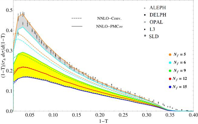
A direct comparison between PMC∞ (solid line) and CSS (dashed line) is shown at different values of the number of flavors. We notice that, despite the phase transition (i.e. the transition from an infrared finite coupling to an infrared diverging coupling), the curves given by the PMC∞ at different , preserve with continuity the same characteristics of the conformal distribution setting out of the conformal window of pQCD. In fact, the position of the peak of the thrust distribution is well preserved varying in and out of the conformal window using the PMC∞, while there is constant shift towards lower values using the CSS. These trends are shown in Fig. 6.2. We notice that in the central range, , the position of the peak is exactly preserved using the PMC∞ and overlaps with the position of the peak shown by the experimental data. According to our analysis for the case PMC∞, in the range, the number of bins is not enough to resolve the peak, though the behavior of the curve is consistent with the presence of a peak in the same position, while for the peak is no longer visible. Theoretical uncertainties on the position of the peak have been calculated using standard criteria, i.e. varying the remaining initial scale value in the range , and considering the lowest uncertainty given by the half of the spacing between two adjacent bins.

Using the definition given in Eq. 5.20, we have determined the average error, , calculated in the interval of thrust and results for CSS and PMC∞ are shown in Fig. 6.3. We notice that the PMC∞ in the perturbative and IR conformal window, i.e. , which is the region where in the whole range of the renormalization scale values, from up to , the average error given by PMC∞ tends to zero () while the error given by the CSS tends to remain constant (). The comparison of the two methods shows that, out of the conformal window, , the PMC∞ leads to a higher precision.
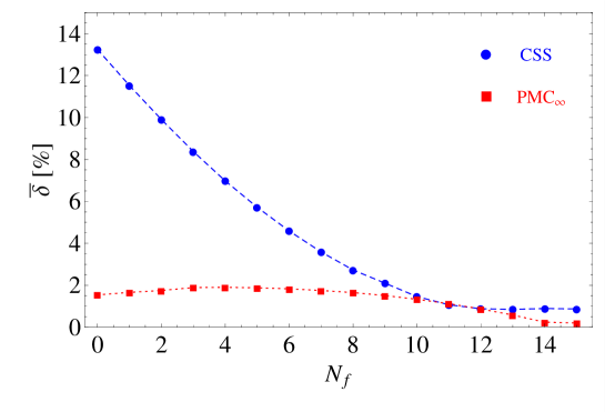
6.2 The thrust distribution in the Abelian limit
We consider now the thrust distribution in U(1) Abelian QED, which rather than being infrared interacting is infrared free. We obtain the QED thrust distribution performing the limit of the QCD thrust at NNLO according to [32, 76]. In the zero number of colors limit the gauge group color factors are fixed by , where is the number of active leptons, while the -terms and the coupling rescale as and respectively. In particular and using the normalization of Eq. 2.8. According to this rescaling of the color factors we have determined the QED thrust and the QED PMC∞ scales. For the QED coupling, we have used the analytic formula for the effective fine structure constant in the -scheme:
| (6.1) |
with and the vacuum polarization function () calculated perturbatively at two loops including contributions from leptons, quarks and boson. The QED PMC∞ scales have the same form of Eqs. 5.21 and 5.26 with the factor for the -scheme set to and the regularization parameter introduced to cancel singularities in the NLO PMC∞ scale in the limit tends to the same QCD value, . A direct comparison between QED and QCD PMC∞ scales is shown in Fig. 6.4.
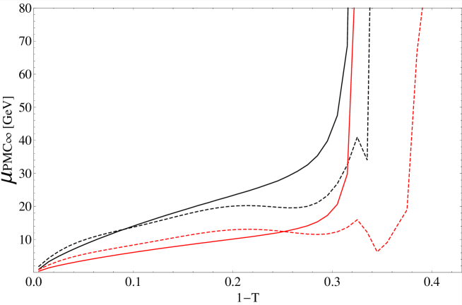
We note that in the QED limit the PMC∞ scales have analogous dynamical behavior as those calculated in QCD, differences arise mainly owing to the scheme factor reabsorption, the effects of the number of colors at NLO are very small. Thus we notice that perfect consistency is shown from QCD to QED using the PMC∞ method. The normalized QED thrust distribution is shown in Fig. 6.5. We note that the curve is peaked at the origin, , which suggests that the three-jet event in QED occurs with a rather back-to-back symmetry. Results for the CSS and the PMC∞ methods in QED are of the order of and show very small differences, given the good convergence of the theory.
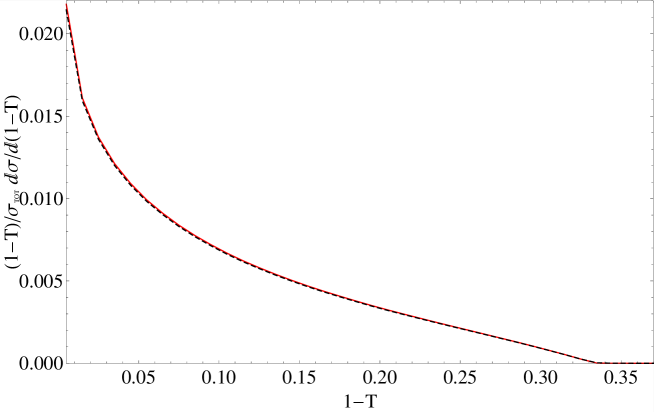
Chapter 7 Precise determination of the strong coupling and its behavior from Event Shape variables using the PMC
In this section we present a novel method for precisely determining the running QCD coupling constant over a wide range of from Event Shape variables for the electron-positron annihilation process measured at a single center-of-mass energy , based on PMC scale setting. In particular, we show results obtained in Refs. [149, 146] using the approach of a single PMC scale at LO and at NLO , i.e. the PMC(LO) of the previous chapter.
The precise determination of the strong coupling is one of the crucial tests of QCD. The dependence of on the renormalization scale obtained from many different physical processes shows consistency with QCD predictions and asymptotic freedom. The Particle Data Group (PDG) currently gives the world average: [152] in the renormalization scheme.
Particularly suitable to the determination of the strong coupling is the process since its lowest order is [127]. Currently, theoretical calculations for event shapes are based on CSS. By using conventional scale setting, only one value of at the scale can be extracted and the main source of the uncertainty is given by the choice of the renormalization scale. Several values for the strong coupling have been extracted from several processes, e.g. [153] is obtained by using perturbative corrections and resummation of the large logarithms at the NNLO+NLL accuracy predictions. Other evaluations improving the resummation calculations up to N3LL give a result of [96] from thrust, and [154] from the C-parameter. Non-perturbative corrections for hadronization effects have also been included in Ref. [155], but as pointed out in Ref. [152], the systematics of the theoretical uncertainties given by hadronization effects are not well understood.
We show in this section that using the PMC is possible to eliminate the renormalization scale ambiguities and obtain consistent results for the strong coupling using the precise experimental data of Event Shape variable distributions. We notice that improved event shape distributions have been obtained in Refs. [23, 148, 156] using BLM and the soft and collinear effective theory (SCET) .
7.1 Running behavior
Given that the PMC scale (PMC(LO)) is not a single-valued but rather a monotonically increasing function of and of the selected observable,(as shown in Figs. 5.1 and 5.4), it is possible to determine the strong coupling values at different scales from one single experiment at one single center-of-mass energy. The dependence of the scale on the observable reflects the dynamics of the underlying gluon and quark subprocess. This dynamics varies also the number of active flavors . Considering that PMC scales for QCD and QED show the same behavior and their relation at LO is only given by a RS redefinition term: this approach can also be extended to QED.
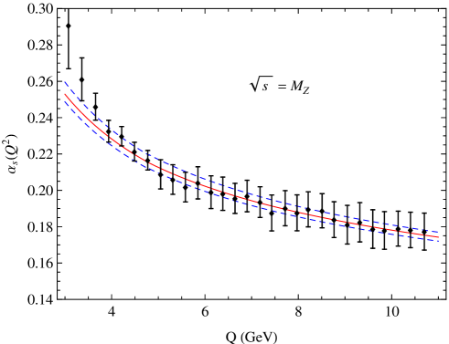
We extract at different scales bin-by-bin from the comparison of PMC predictions for () and differential distributions with measurements at . The extracted values from the C-parameter distribution are shown in Fig. 7.1. We note that the extracted in the scale range of GeV GeV are in excellent agreement with the world average evaluated from [152]. Given that the PMC scale setting eliminates the scale uncertainties, the corresponding extracted values are not plagued by any ambiguity in the choice of . The extracted values from the thrust observable using PMC are shown in Fig. 7.2. Also in this case there is good agreement in the range GeV GeV (corresponding to the () range: ). These extracted values of are in good agreement also with the world average value of the PDG [152].
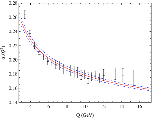
Thus, PMC scale setting provides a remarkable way to verify the running of from event shapes measured at a single energy of . Analogously in QED, the running of QED coupling can be measured at a single energy of (see e.g. [157]).
The differential distributions of event shapes are afflicted with large logarithms especially in the two-jet region. Thus, the comparison of QCD predictions with experimental data and thus the extracted values are restricted to the region where the theory is able to describe the data well.
Choosing a different area of distributions leads to the different values of .
7.2 from mean values
The mean value of an event shape defined by:
| (7.1) |
where is the kinematically allowed upper bound of the variable, involves an integration over the full phase space, it thus provides an important platform to complement the differential distributions and to determinate .
The mean values of event shapes have been extensively measured and studied. At the present moment, pQCD predictions including NNLO QCD corrections [158, 159] based on CSS substantially underestimate experimental data.
PMC scales for the mean values of the event shapes are respectively:
for thrust and the C-parameter. Both PMC scales are .
When taking GeV, the PMC scales are GeV and GeV for the thrust and the C-parameter, respectively. The PMC scales of the differential distributions for the thrust and the C-parameter are also very small. The average of the PMC scales of the differential distributions for the thrust and the C-parameter are close to the PMC scales and , respectively. This shows that PMC scale setting is self-consistent from the differential distributions to the mean values.
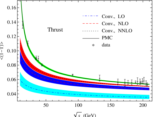
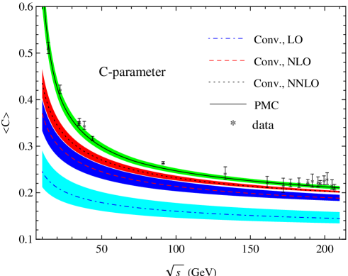
The results for the mean values of thrust and the C-parameter versus the center-of-mass energy are shown in Fig. 7.3. We note that the results obtained with conventional scale setting substantially deviate from experimental data. In contrast, PMC scale setting leads to improved mean values results for both thrust and the C-parameter. PMC predictions are in excellent agreement with experimental data over a wide range of energies.
We point out that PMC predictions eliminate the scale uncertainty thus errors estimated with the standard criteria are almost negligible. A better estimate of the unknown higher-order terms can be obtained by analyzing the magnitude of the perturbative corrections and the convergence of the series.
The relative magnitude of corrections for the C-parameter distribution is [141] in the intermediate region using CSS. Using the PMC, the relative magnitude at NLO is improved to be . The error estimate of an th-order calculation for the unknown term can be characterized by the last known term, i.e., , where stands for LO, NLO, NNLO, . The unknown term can be reasonably estimated assuming the same rate of increment of the last known order, . Hence, in this case, we have that error bars are given by: (as shown in Fig. 7.3).
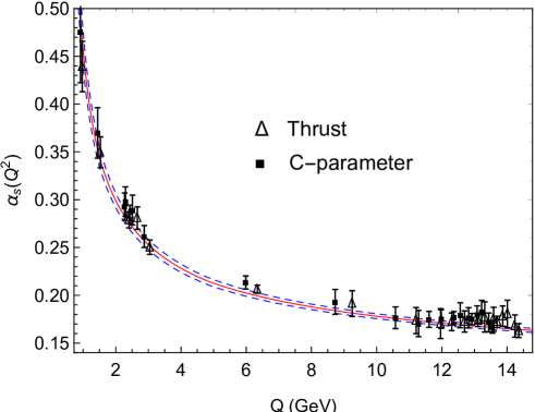
Given the high level of agreement of the PMC predictions with the measurements, we can extract to a very high precision.
Results are shown in Fig. 7.4. We notice an excellent agreement of the values with the world average in the scale range of .
The extracted are not plagued by the scale uncertainty. In addition, unlike the extracted from the differential distributions, the extracted from the mean values are not afflicted with the large logarithms nor the non-perturbative effects.
7.3 from -fit
In order to obtain a reliable at the scale of the mass, we determine from the fit of the PMC predictions to measurements. In particular, we perform the fit by minimizing the respect to the parameter. The variable is defined as:
where is the value of the experimental data, is the corresponding experimental uncertainty and is the theoretical prediction. The fit for thrust and the C-parameter leads to the results:
| (7.2) | |||||
with d.o.f. for the thrust mean value, and
| (7.3) | |||||
with d.o.f. for the C-parameter mean value, where the first error is the experimental uncertainty and the second error is the theoretical uncertainty. Both results are consistent with the world average of [152].
The precision of the extracted has been greatly improved by using the PMC: the dominant scale uncertainties are eliminated and the convergence of pQCD series is greatly improved. In particular, a strikingly much faster pQCD convergence is obtained for the thrust mean value [146], theoretical uncertainties are even smaller than the experimental uncertainties. We remark that these results for are one of the most precise determinations of strong coupling at the mass from event shape variables.
Chapter 8 Heavy-quark pair production near the threshold region
Heavy fermion pair production in annihilation near the threshold region is a fundamental process for the Standard Model and of considerable interest for various phenomena. The precise prediction of the production cross section for at the threshold region is important in order to improve the measurement of the -lepton mass [161]. Precise theoretical predictions for the production cross section of at the thresholds are also crucial to determine the precise values of the quark mass and of the coupling constant determined by the sum rule method [162, 163, 164].
For the physics of the future high-energy electron-positron colliders, one of the most important goals is the precise measurement of top-quark properties, especially the top quark mass and width in the threshold region [165]; in order to reach the aimed precision, precise predictions for the top-quark pair production cross section are mandatory.
For heavy-fermion pair production in annihilation, it is well known that the Coulomb correction appears near the threshold region, and the fixed-order perturbative calculations are spoilt by the presence of singular terms. Physically, the renormalization scale should become very soft in this region. However, the renormalization scale is usually set to the mass of the heavy fermion for the calculation of the production cross sections using standard CSS. Results are then affected by systematic errors, due to inherent scheme and scale uncertainties, and predictions are quite unreliable in this kinematic region. In this chapter, we apply the PMC to make a comprehensive analysis for heavy-fermion pair production in annihilation near the threshold region. We show that two distinctly different scales are determined for heavy fermion pair production near the threshold region and we show consistency of PMC scale setting with QED. For the purpose we show the results in both the modified minimal subtraction scheme ( scheme) and the V-scheme and we compare the results with the QED GM-L scheme.
8.1 The QCD process of the quark pair production in the scheme
The interaction between two heavy quarks can be described at threshold by considering separate contributions arising from non-relativistic and hard processes dynamics. Non-relativistic contributions are determined by a non-relativistic potential that is essentially the result of the effects of a static Coulomb-like potential and of the linearly diverging confining term. While the hard contributions encompass virtual perturbative QCD corrections between heavy quarks in the final state. At the threshold, kinematic boundaries enhance the effects of the Coulomb non-relativistic terms that become large. Thus, we can distinguish two typologies of perturbative corrections for the heavy quark pair production cross section that we label as Coulomb and non-Coulomb corrections. The cross section for is known at two-loop level (Ref. [166]) and it is given by:
| (8.1) |
where , is the renormalization scale. The LO cross section is
| (8.2) |
and the quark velocity is
| (8.3) |
Here, is the number of colors, is the quark electric charge, is the center-of-mass energy squared and is the mass of the heavy quark . The one-loop correction near the threshold region can be written as
| (8.4) |
The two-loop correction can be conveniently split into terms proportional to various color factors,
| (8.5) | |||||
The terms , and are the same in either Abelian or non-Abelian theories; the term only arises in the non-Abelian theory. This process provides the opportunity to explore rigorously the scale-setting method in non-Abelian and Abelian theories.
The Coulomb corrections play an important role in the threshold region, since they are proportional to powers of . This implies that the renormalization scale can be relatively soft in this region. Thus the PMC scales must be determined separately for the non-Coulomb and Coulomb corrections [107, 27]. When the quark velocity , the Coulomb correction dominates the contribution of the production cross section, and the contribution of the non-Coulomb correction will be suppressed.
From general grounds, one expects threshold physics to be governed by the non-relativistic instantaneous potential.
The potential affects the cross section through final state interactions when the scale is above threshold; it leads to bound states when the scale is below threshold.
In order to apply the PMC, we write explicitly the -dependent and -independent parts in the Eq. 8.1, i.e.,
| (8.6) | |||||
The coefficients and are for the non-Coulomb corrections, and the coefficients , and are for the Coulomb corrections. These coefficients in the scheme are calculated in Refs. [166, 167, 168] and at the scale they can be written as
| (8.7) | |||||
| (8.8) |
After absorbing the nonconformal term into the coupling constant using the PMC, we achieve:
| (8.9) | |||||
The PMC scales can be written as
| (8.10) |
and the coefficients are
| (8.11) |
where, and stand for the non-Coulomb and Coulomb corrections, respectively. The nonconformal term is eliminated, and the resulting pQCD series matches the conformal series and thus only the conformal coefficients remain in the cross section. The conformal coefficients are independent of the renormalization scale . At the present two-loop level, the PMC scales are also independent of the renormalization scale . Thus, the resulting cross section in Eq. 8.9 eliminates the renormalization scale uncertainty.
Considering the color factors , and for QCD, the PMC scales in the scheme are
| (8.12) |
for the non-Coulomb correction, and
| (8.13) |
for the Coulomb correction. The scale stems from the hard gluon-virtual corrections, and thus it is determined from the short-distance process. The scale originates from the static Coulomb potential. As expected, the scale is of order , while the scale is of order .

In the following, we take bottom-quark pair production as an example to make a detailed analysis near the threshold region. Taking GeV [170], we obtain
| (8.14) |
which is smaller than in the scheme. For the Coulomb correction part, the scale is shown in Fig. 8.1. It shows that the scale depends continuously on the quark velocity , and becomes soft for , yielding the correct physical behavior of the scale and reflecting the virtuality of the QCD dynamics. Also the number of active flavors changes with the quark velocity according to the PMC scale.
When the quark velocity , the small scale in the coupling constant shows that the perturbative QCD theory becomes unreliable and non-perturbative effects must be taken into account. One can adopt light-front holographic QCD [80] to evaluate in the low-scale region.
In contrast, the renormalization scale is simply fixed to the typical scale using CSS. Our calculations show that in the scheme, the scale should be , which is smaller than for the non-Coulomb correction. For the Coulomb correction, simply fixing the renormalization scale obviously violates the physical behavior near the threshold region, since the scale becomes soft for .
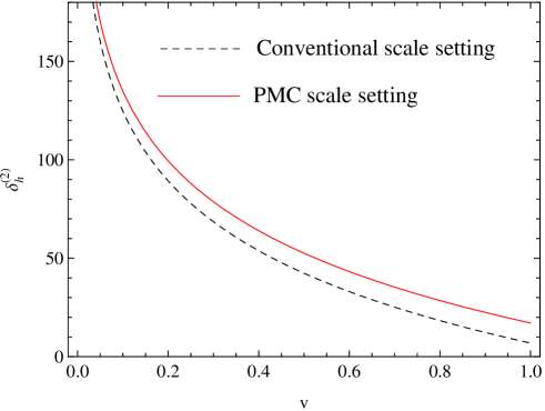
The two-loop coefficients of the non-Coulomb correction in the scheme using conventional and PMC scale settings are shown in Fig. 8.2. We note that although the -dependent behavior of the coefficients is the same, their magnitudes are different using different scale settings. When the quark velocity , both curves diverge due to the presence of the term . As expected, after multiplying this term by the -factor in the LO cross section given in Eq. 8.2, the contribution of the non-Coulomb corrections is finite and is suppressed near the threshold region, i.e. for the quark velocity .
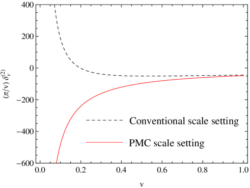
In the small relative velocity domain, i.e. , the effect of multiple-photon exchange between charged particles becomes significant.
It was shown by Sommerfeld that the correction due to re-scattering of charged particles in the final state is proportional to the wave function at the origin squared, . Thus, the annihilation process acquires some characteristics of the corresponding bound state. It was shown by Gamow-Sommerfeld-Sakharov [171, 172, 173] that the leading contributions can be resummed using the so-called SGS factor:
| (8.15) |
with . Thus the Coulomb term of the form can be reabsorbed in the Sommerfeld rescattering formula [166].111It is also believed that the subleading terms can be resummed by adding a hard coefficient factor, such as:
For the Coulomb term of the form , we present the coefficients in the scheme using conventional and PMC scale settings in Fig. 8.3. It shows that when the quark velocity , the -dependent behavior of the coefficients is dramatically different using conventional and PMC scale settings. In the case of conventional scale setting, its behavior is for due to the presence of the term . After multiplying this term by the -factor in the LO cross section , the contribution of the Coulomb correction using conventional scale setting is not finite, i.e., for . It should be stressed that the term vanishes, and the term remains in the conformal coefficient after applying PMC scale setting. Thus the -dependent behavior is for . This term is cancelled by multiplying it by the -factor in the LO cross section , and thus the contribution of the Coulomb correction using PMC scale setting is finite for . For , contributions of the Coulomb correction using conventional and PMC scale settings are both suppressed.
8.2 Quark-pair production in the V-scheme
In order to investigate possible scheme dependence effects, we perform the above analysis also in a different scheme. Particularly suitable for the purpose is the scheme defined by the effective charge (V-scheme) given by the static potential between two heavy quarks [69, 70, 71, 72, 73, 74, 75],
| (8.16) |
which provides a physically-based alternative to the usual scheme. Analogously to QED and the GM-L scheme, setting the scale to the virtuality of the exchanged gluon, all vacuum polarization corrections are resummed into the coupling . By using the relation between and at the one-loop level, i.e.,
| (8.17) |
we can perform the change of scheme for Eq. 8.6, from the scheme to the V-scheme. Thus, the corresponding perturbative coefficients in the V-scheme are:
| (8.18) |
| (8.19) | |||||
| (8.20) |
And the corresponding PMC scales in the V-scheme are:
| (8.21) |
for the non-Coulomb correction, and
| (8.22) |
for the Coulomb correction. Again, in the V-scheme, is of order , while is of order , since the scale originates from the hard-gluon virtual corrections, and originates from Coulomb rescattering. The physical behavior of the scales does not change using different renormalization schemes. We notice that the difference between the PMC scales in the scheme and in the physically-based V-scheme is given by scheme factor. This difference is unphysical and is a consequence of the particular convention adopted.
The PMC scale eliminates this conventional dependence (i.e. this RS dependence). Scheme independent relations between two effective charges can be achieved by “commensurate scale relations” (CSR) [108, 86] as discussed in Sec.3.

For -quark production, setting the mass to GeV, we obtain the scale GeV for the non-Coulomb correction, and its value larger than the conventional choice . The scale for the Coulomb correction depends on the velocity , we show the scale versus the center-of-mass energy in the V-scheme in Fig. 8.4. The exponent disappears in Eq. 8.22 compared to the scale in Eq. 8.13 in the scheme. The scale becomes soft for , and for , showing the correct physical behavior.

As in the case of the scheme, the -dependent behavior of the coefficients of the non-Coulomb correction in the V-scheme using conventional and PMC scale settings is the same. The two-loop coefficients of the Coulomb correction in the V-scheme using conventional and PMC scale settings are presented in Fig. 8.5. Figure 8.5 shows that close to the threshold region, the -dependent behavior of the coefficients using conventional and PMC scale settings is dramatically different. When the quark velocity , the coefficient is due to the presence of the term using conventional scale setting. After applying PMC scale setting, the coefficient is due to the term vanishes and the term remains in the conformal coefficient. Thus, multiplying by the -factor in the LO cross section , the contribution of the Coulomb correction for is not finite using conventional scale setting and is finite after using PMC scale setting. It is noted that quark-pair and lepton-pair production in annihilation near the threshold region should show similar physical behavior. This dramatically different behavior of the between conventional and PMC scale settings near the threshold region should be checked in QED.
8.3 Lepton pair production
Similar to quark-pair production, the lepton-pair production cross section for the QED process is expanded in the QED fine structure constant . According to the previous analysis, we can split the cross section into non-Coulomb and Coulomb parts. Perturbative coefficients for the lepton-pair production cross section can be obtained from Eq. 8.6 by replacing the QCD color factors: , and with the corresponding QED [166, 174, 175]: , and .
Applying the PMC, vacuum-polarization corrections can be absorbed into the QED running coupling, according to:
| (8.23) |
where is the mass of the light virtual lepton, and is far smaller than the final-state lepton mass .
The resulting PMC scales can be written as
| (8.24) |
where, and stand for the non-Coulomb and Coulomb corrections, respectively. After absorbing the vacuum polarization corrections into the QED running coupling, the coefficients vanish. According to the replacements , and for QED, the PMC scales become:
| (8.25) |
for the non-Coulomb correction, and
| (8.26) |
for the Coulomb correction.
PMC scales show the same physical behavior from QCD to QED. It is noted that PMC scales in Eqs. 8.21 and 8.22 for QCD in the V-scheme coincide with the QED scales in Eqs. 8.25) and 8.26, respectively. This result was expected for self-consistency, given that the PMC method in QCD agrees with the standard Gell-Mann-Low method [4] in QED. We also point out that the V-scheme provides a natural scheme for the QCD process for quark-pair production.
In the following, we take -lepton pair production as an example to make a detailed analysis near the threshold region. Taking GeV [152], we obtain the scale GeV, which is larger than the scale for non-Coulomb correction. For the Coulomb correction, as in the case of QCD, the scale becomes soft for and for . The PMC scales thus rigorously yield the correct physical behavior for the lepton pair production near the threshold region.
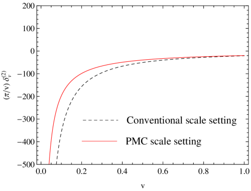
Non-Coulomb corrections have the same -dependent behavior for the coefficients independently of the use of conventional or PMC scale settings, as for the QCD case. For the Coulomb correction, we show the coefficients using conventional and PMC scale settings in Fig. 8.6.
It is noted that in contrast with the QCD case, using the CSS, when the quark velocity , the coefficient due to the presence of the term ; while using the PMC the coefficient due to the presence of the term . Multiplying by the -factor in the LO cross section , the contribution of the Coulomb correction is given by: for using conventional scale setting, and is a finite for using PMC scale setting. We note that using different scale setting we achieve opposite behaviors, as shown in Figs. 8.3, 8.5 and 8.6, but only the PMC is in agreement with the QED results of the GM-L scheme. Moreover, scale setting affects results for the Coulomb corrections that are finite when using the PMC scale setting, and in contrast diverge when using conventional scale setting for both QCD and QED.
Summary
We briefly summarize here the results.
-
I)
In section 5 we have illustrated the PMC∞ method and how it applies to either numerical or analytical calculated observables. The approach of the PMC∞ is totally general and can be applied to any perturbative calculation, such as fully integrated cross sections and also differential distributions. This new approach preserves intrinsic conformality (iCF), which introduces a new concept of scale invariance: ordered scale invariance, i.e. the scale invariance of any combination of conformal subsets. In this approach scale invariance is preserved perturbatively, analogously to gauge invariance.
In this thesis we have also presented a new procedure to identify the conformal coefficients and the PMC∞-scales valid to all orders, which can be applied to either numerical or analytical calculations. The PMC∞ preserves the (A,B,C,D,E,F) properties of the BLM/PMC method: it eliminates renormalon growth , scheme dependence and all uncertainties related to the scale ambiguity up to the order of accuracy. The iCF/PMC∞ scales are identified by the lowest order logarithm related to the -term at each order and all the physics of the process is contained in the conformal coefficients. This is in complete agreement with QED and with the Gell-Mann and Low scheme [17, 32].
We have discussed why iCF should be considered a strict requirement for a theory in order to preserve the scale invariance of the observables and we have shown that iCF is consistent with the single-variable thrust and C-parameter distributions. We point out that other conformal aspects of QCD resulting from different sectors such as Commensurate Scale Relations-CSR [86] or dual theories as AdS/CFT [176] might also be related to the intrinsic conformality.
We underline that the iCF property in a theory would have two main remarkable consequences: first, it indicates the correct coupling constant at each order as a function of the intrinsic conformal scale , and second, since only the conformal and the coefficients need to be identified in the observables at each order, by means of the PMC∞ method the iCF would reveal its predictive feature for the coefficients of the higher order color factors. We point out that in many cases implementation of the iCF in a multi-loop calculations procedure would lead to a significant reduction of the color-factor coefficients and it would speed up the calculations for higher order corrections.
-
II)
In section 5.5 we have shown results for thrust and the C-parameter for , comparing the two methods for setting the renormalization scale in pQCD: the Conventional Scale Setting (CSS) and the infinite-order scale setting based on the Principle of Maximum Conformality (PMC∞). The PMC∞ has been applied to the NNLO thrust and C-parameter distributions and the results show perfect agreement with the experimental data. The evaluation of theoretical errors using standard criteria show that the PMC∞ significantly improves the theoretical predictions over the entire spectra of the shape variables. We have shown that PMC∞ works particularly well for the case of the event shape variables, where we found an extremely good agreement of the coefficients with the iCF parametrization. We point out that in fixed order calculations the PMC∞ last scale is set to the kinematic scale of the process: in this case . As shown in Eq. 5.6, the scale dependence on the initial scale is totally confined in the last subset . Thus the the last term in the iCF determines the level of conformality reached by the expansion and is entangled with theoretical uncertainties given by higher order uncalculated terms. Any variation of the last scale has to be intended to evaluate theoretical uncertainties given by higher order contributions and not as an ambiguity of the PMC∞ method [177]. Evaluation of the theoretical errors using standard criteria shows that the PMC∞ significantly improves the precision of the pQCD calculations for thrust and C-parameter. We remark that an improved analysis of theoretical errors might be obtained by giving a prediction of the contributions of higher order terms using a statistical approach as shown in Refs. [178, 179]. This would lead to a more rigorous method to evaluate errors and thus to restrict the range of the last PMC∞ scale that, as we have shown here, can also be fixed to the last known PMC∞ one leading to precise and stable predictions.
-
III)
In section 6 we have investigated, for the first time, the thrust distribution in the conformal window of pQCD and in the QED limit. Assuming, for phenomenological reasons, the physical value of the strong coupling to be that of the mass scale, it restricts the conformal window range, at two loops, to be within with . The closer is to the higher value, the more perturbative and conformal the system is. In this region, we have shown that the PMC∞ leads to a higher precision with a theoretical error that tends to zero. Moreover, results for the thrust distribution in the conformal window have similar shapes to those of the physical values of and the position of the peak is preserved when one applies the PMC∞ method. Comparison with the experimental data indicates also that PMC∞ agrees with the expected number of flavors. A good fit with experimental data is shown by the PMC∞ results for the range , which agrees with the active number of flavors of the Standard Model. Outside the pQCD conformal window the PMC∞ leads to a higher precision with respect to the CSS. In addition, calculations for the QED thrust shown in section 6.2 reveal a perfect consistency of the PMC∞ with QED when taking the QED limit of QCD for both the PMC∞ scale and for the regularization parameter which tends to the same QCD value.
-
IV)
In section 7 we have presented a novel method to determine the strong coupling constant from event-shape variables. Though the event-shape variables, especially those for the process , are particularly suitable for the determination of the strong coupling constant , results obtained by using CSS do not match the experimental average value and event-shape distributions underestimate the experimental data at NNLO. Some extracted from event shapes by the CSS may also seem quite unrealistic. Our analysis suggests that these conventional difficulties can be overcome by using the PMC renormalization scale setting leading to a comprehensive and self-consistent analysis for both the differential distributions and the mean values for event shapes. The physical observable should be independent of the choice of renormalization scale. The PMC scale yields the renormalization scale-independent physical behavior and reflects the virtuality of the QCD dynamics. Thus the PMC provides a remarkable way to verify the running of from the event shape differential measurement at a single energy of . The values of determined are consistent with the world average and are more precise than the values obtained from previous analysis performed on the same data. Recently in Ref. [180], this method has also been extended to the other event-shape variables .
-
V)
In section 8 we have investigated heavy-fermion pair production in annihilation as a fundamental process of the SM. In the kinematic region close to threshold, two major distinct contributions arise in perturbative calculations given by the static Coulomb-like rescattering potential and non-Coulomb hard-gluon virtual corrections. The conventional procedure of simply setting the renormalization scale as violates the physical behavior and leads to unreliable predictions near the threshold region. In contrast, the PMC scale-setting method provides a self-consistent analysis, and reveals perfect agreement for the physical behavior of the scale near the threshold region, between QED and QCD. This fundamental process shows a peculiar situation where two distinctly different scales are applied using the PMC. The scale determined for the hard virtual correction is of order the fermion mass ; the scale determined for the Coulomb rescattering is of order , which becomes soft at the threshold, given that . This reflects the physical virtuality of the exchanged gluons (or photons), given by the dynamics of the underlying physical QCD (or QED) process.
-
•
While non-Coulomb corrections for fermion pair production are suppressed near the threshold region, the Coulomb corrections diverge in this kinematic region, using CSS. In contrast, the -dependent behavior of the scale changes after using PMC scale setting, turning into a perfectly consistent behavior from QCD to QED. The divergence is given only by the higher-order -Coulomb terms, and the proper resummation using the Sommerfeld (SGS) rescattering formula leads to a finite result. A finite prediction can also be obtained using the PMC scale setting in both QCD and in QED.
-
•
A straight comparison between QED and QCD is obtained using the V-scheme, which provides a natural scheme for the QCD calculation for the quark pair production process. Converting the QCD calculations in the scheme to the V-scheme, the resulting PMC predictions in the QED limit are consistent with the GM-L scheme. QCD and QED scales differ only by a scheme factor: ; this factor converts the underlying scale predictions in the scheme used in QCD to the scale of the V-scheme conventionally used in QED [108]. In fact, the PMC scales are: for the hard virtual correction and for Coulomb rescattering for both QCD and QED. The predictions in the V-scheme based on the conventional scale-setting method do not agree with the QED limit where the renormalization scale can be set unambiguously by using the GM-L method. The PMC scale-setting method in QCD can be reduced in the Abelian limit to the Gell-Mann-Low method. This consistency provides strong support for the PMC scale-setting method.
Conclusions
In this thesis we have introduced a new scale setting procedure, namely PMC∞, which stems from the general Principle of Maximum Conformality (PMC) and preserves a particular property that we have defined as intrinsic conformality (iCF). The iCF is a particular parametrization of the perturbative series that preserves exactly the scale invariance of an observable perturbatively. The PMC∞ solves the conventional renormalization-scale ambiguity in QCD, it preserves not only the iCF but also all the features of the PMC approach and leads to a final conformal series at any order of the perturbative calculation. In fact, the final series is given by perturbative conformal coefficients with the couplings determined at conformal renormalization scales. This method agrees with the BLM/PMCm approach at LO and given the uniqueness of the iCF, any other alternative method, e.g. the method proposed in Ref. [177], which we indicate as “PMCa”, to fix a scale in order to obtain a perturbative scale-invariant quantity leads to the same results as the PMC∞, as shown in Ref. [181]. Unlike the previous BLM/PMC approaches, the PMC∞ scales are not perturbatively calculated, but are conformal functions of the physical scale/scales of the process and any other non-integrated momentum/variable, e.g. the event-shape variable or .
The PMC∞ is totally independent of the initial scale used for renormalization in perturbative calculations and it preserves the scale invariance at any stage of calculation, independently of the kinematic boundary conditions, independently of the starting order of the observable or the order of the truncated expansion.
The iCF improves the general BLM/PMC procedure and the point “3” of section 3.4. In the same section, we have suggested that an improvement and simplification of the perturbatively calculated BLM/PMC scales, would be achieved by setting the renormalization scale directly to the physical scale Q of the process, before applying the BLM/PMC procedure. This would remove the initial scale dependence from the perturbatively calculated BLM/PMC scales.
We underline that in contrast with the other PMCm and PMCs approach the PMC∞ preserves the iCF, thus scales are set automatically in kinematic regions where kinematic constraints cancel the effects of the lower order conformal coefficients. These effects are particularly visible in the case of event-shape variables in the multi-jet regions. The iCF effects in these kinematic regions are neglected by the PMCm and PMCs approach, unless an ad hoc prescription is introduced. As recently shown in Refs. [182] and [181], application of the PMC∞ improves the theoretical predictions for , , , with respect to the CSS. It has been noted in Ref. [181] that in general also the PMCs approach works remarkably well especially for fully integrated quantities.
We point out that this approach may have an effect of averaging the differences of the PMCm/PMC∞ scales arising at each order, which might be significant for the precision of a prediction at a certain level of accuracy.
However, given the small differences that we have found in the first two consecutive PMC∞ scales, i.e. , in the LO allowed kinematic region, i.e. and in , we may argue that in the same accessible kinematic domain two consecutive PMC∞ scales have such small differences that a single-scale approach, such as the PMCs, would be justified leading to analogously precise predictions.
We recall that only the terms related to the UV diverging diagrams (i.e. the terms) must be reabsorbed into the PMC∞ scales. Thus PMC∞ perfectly agrees with the PMCm when an observable has a manifest iCF form. We remark that the iCF underlies scale invariance perturbatively, i.e. the ordered scale invariance. We also remark that PMC∞ agrees with the single-scale approach PMCs in the case of an observable with a particular iCF form with all scales equal, i.e. . In this sense the PMCm and PMCs may be considered more as “optimization procedures” that follow the purpose of the maximal conformal series by transforming the original perturbative series into an iCF-like final series by using the PMC scales. In contrast, the PMC∞ does not indicate any particular value of the renormalization scale to be used, but indicates the final limit obtained by each conformal subset and then by the perturbative expansion once all the terms related to each conformal subset are resummed. The PMC∞ is RG invariant at each order of accuracy, which means we can perform a change of scale at any stage and reobtain the initial perturbative quantity. In this sense PMC∞ is not to be understood as an “optimization procedure”, but as an explicit RG invariant form to parametrize a perturbative quantity that leads faster to the conformal limit. By setting the renormalization scale of each subset to the corresponding PMC∞ scale, one simply cancels the infinite series of terms, leading to the same conformal result as the original series. Given that both scales and coefficients are conformal in the PMC∞, also the scheme and scale dependence is completely removed in the perturbative series up to infinity. It has been pointed out in Ref. [181], that the PMC∞ scale might become quite small at a certain order and that PMC∞ retains the second kind of scale dependence. We underline that the last scale in the PMC∞ controls the level of convergence and the conformality of the perturbative series and is thus entangled with the theoretical error of a given prediction. According to the PMC∞ procedure the last scale must be set to the invariant physical scale of the process, given by . We have shown in this thesis that the usual PMC practice of setting the last scale equal to the last unknown scale is consistent also for the PMC∞ and leads to precise and stable results. At the moment, improvements to these points are under investigation.
We remark that the evaluation of the theoretical errors using standard criteria, shows that the PMC∞ significantly improves the precision of the pQCD calculations and eliminates the scheme and scale ambiguities. An improved analysis of theoretical errors might be obtained by using a statistical approach for evaluating the contributions of the uncalculated higher order terms as shown in Refs. [178, 179]. This approach would lead to a more rigorous method to evaluate errors giving also indications on the possible range of values for the last unknown PMC∞ scale.
References
- [1] Charalampos Anastasiou, Claude Duhr, Falko Dulat, Elisabetta Furlan, Thomas Gehrmann, Franz Herzog, Achilleas Lazopoulos, and Bernhard Mistlberger. High precision determination of the gluon fusion Higgs boson cross-section at the LHC. JHEP, 05:058, 2016.
- [2] Stefano Catani, Simone Devoto, Massimiliano Grazzini, Stefan Kallweit, and Javier Mazzitelli. Bottom-quark production at hadron colliders: fully differential predictions in NNLO QCD. JHEP, 03:029, 2021.
- [3] Ernst Carl Gerlach Stueckelberg de Breidenbach and Andreas Petermann. Normalization of constants in the quanta theory. Helv. Phys. Acta, 26:499–520, 1953.
- [4] Murray Gell-Mann and F. E. Low. Quantum electrodynamics at small distances. Phys. Rev., 95:1300–1312, 1954.
- [5] A. Peterman. Renormalization Group and the Deep Structure of the Proton. Phys. Rept., 53:157, 1979.
- [6] Curtis G. Callan, Jr. Broken scale invariance in scalar field theory. Phys. Rev. D, 2:1541–1547, 1970.
- [7] K. Symanzik. Small distance behavior analysis and Wilson expansion. Commun. Math. Phys., 23:49–86, 1971.
- [8] William Celmaster and Richard J. Gonsalves. The Renormalization Prescription Dependence of the QCD Coupling Constant. Phys. Rev. D, 20:1420, 1979.
- [9] Andrzej J. Buras. Asymptotic Freedom in Deep Inelastic Processes in the Leading Order and Beyond. Rev. Mod. Phys., 52:199, 1980.
- [10] Paul M. Stevenson. Resolution of the Renormalization Scheme Ambiguity in Perturbative QCD. Phys. Lett. B, 100:61–64, 1981.
- [11] Paul M. Stevenson. Optimized Perturbation Theory. Phys. Rev. D, 23:2916, 1981.
- [12] Paul M. Stevenson. Optimization and the Ultimate Convergence of QCD Perturbation Theory. Nucl. Phys. B, 231:65–90, 1984.
- [13] P. Stevenson. Sense and Nonsense in the Renormalization Scheme Dependence Problem. Nucl. Phys. B, 203:472–492, 1982.
- [14] G. Grunberg. Renormalization Group Improved Perturbative QCD. Phys. Lett. B, 95:70, 1980. [Erratum: Phys.Lett.B 110, 501 (1982)].
- [15] G. Grunberg. Renormalization Scheme Independent QCD and QED: The Method of Effective Charges. Phys. Rev. D, 29:2315–2338, 1984.
- [16] G. Grunberg. On Some Ambiguities in the Method of Effective Charges. Phys. Rev. D, 40:680, 1989.
- [17] Stanley J. Brodsky, G. Peter Lepage, and Paul B. Mackenzie. On the Elimination of Scale Ambiguities in Perturbative Quantum Chromodynamics. Phys. Rev. D, 28:228, 1983.
- [18] L. F. Abbott. Choosing an Expansion Parameter for QCD. Phys. Rev. Lett., 44:1569, 1980.
- [19] G. ’t Hooft. The Whys of Subnuclear Physics. In Proc. Intern. School of Subnuclear Physics (Erice, 1977 ), page 943. ed. A. Zichichi (Plenum, New York, 1979).
- [20] C. F. Berger, Z. Bern, Lance J. Dixon, Fernando Febres Cordero, D. Forde, T. Gleisberg, H. Ita, D. A. Kosower, and D. Maitre. Next-to-Leading Order QCD Predictions for W+3-Jet Distributions at Hadron Colliders. Phys. Rev. D, 80:074036, 2009.
- [21] Xing-Gang Wu, Stanley J. Brodsky, and Matin Mojaza. The Renormalization Scale-Setting Problem in QCD. Prog. Part. Nucl. Phys., 72:44–98, 2013.
- [22] Alexandre Deur, Stanley J. Brodsky, and Guy F. de Teramond. The QCD Running Coupling. Nucl. Phys., 90:1, 2016.
- [23] G. Kramer and B. Lampe. Jet production rates at LEP and the scale of alpha-s. Z. Phys. A, 339:189–193, 1991.
- [24] Stanley J. Brodsky and Xing-Gang Wu. Self-Consistency Requirements of the Renormalization Group for Setting the Renormalization Scale. Phys. Rev. D, 86:054018, 2012.
- [25] Stanley J. Brodsky and Leonardo Di Giustino. Setting the Renormalization Scale in QCD: The Principle of Maximum Conformality. Phys. Rev. D, 86:085026, 2012.
- [26] Stanley J. Brodsky and Xing-Gang Wu. Scale Setting Using the Extended Renormalization Group and the Principle of Maximum Conformality: the QCD Coupling Constant at Four Loops. Phys. Rev. D, 85:034038, 2012. [Erratum: Phys.Rev.D 86, 079903 (2012)].
- [27] Stanley J. Brodsky and Xing-Gang Wu. Eliminating the Renormalization Scale Ambiguity for Top-Pair Production Using the Principle of Maximum Conformality. Phys. Rev. Lett., 109:042002, 2012.
- [28] Matin Mojaza, Stanley J. Brodsky, and Xing-Gang Wu. Systematic All-Orders Method to Eliminate Renormalization-Scale and Scheme Ambiguities in Perturbative QCD. Phys. Rev. Lett., 110:192001, 2013.
- [29] Stanley J. Brodsky, Matin Mojaza, and Xing-Gang Wu. Systematic Scale-Setting to All Orders: The Principle of Maximum Conformality and Commensurate Scale Relations. Phys. Rev. D, 89:014027, 2014.
- [30] Xing-Gang Wu, Yang Ma, Sheng-Quan Wang, Hai-Bing Fu, Hong-Hao Ma, Stanley J. Brodsky, and Matin Mojaza. Renormalization Group Invariance and Optimal QCD Renormalization Scale-Setting. Rept. Prog. Phys., 78:126201, 2015.
- [31] Xing-Gang Wu, Jian-Ming Shen, Bo-Lun Du, Xu-Dong Huang, Sheng-Quan Wang, and Stanley J. Brodsky. The QCD renormalization group equation and the elimination of fixed-order scheme-and-scale ambiguities using the principle of maximum conformality. Prog. Part. Nucl. Phys., 108:103706, 2019.
- [32] Stanley J. Brodsky and Patrick Huet. Aspects of SU(N(c)) gauge theories in the limit of small number of colors. Phys. Lett. B, 417:145–153, 1998.
- [33] Stanley J. Brodsky, John R. Ellis, Einan Gardi, Marek Karliner, and Mark. A. Samuel. Pade approximants, optimal renormalization scales, and momentum flow in Feynman diagrams. Phys. Rev. D, 56:6980–6992, 1997.
- [34] P. A. Zyla et al. Review of Particle Physics. PTEP, 2020(8):083C01, 2020.
- [35] Keith A. Brueckner. Meson-Nucleon Scattering and Nucleon Isobars. Phys. Rev., 86:106–109, 1952.
- [36] Michael E. Peskin and Daniel V. Schroeder. An Introduction to quantum field theory. Addison-Wesley, Reading, USA, 1995.
- [37] Yan-Rui Liu, Hua-Xing Chen, Wei Chen, Xiang Liu, and Shi-Lin Zhu. Pentaquark and Tetraquark states. Prog. Part. Nucl. Phys., 107:237–320, 2019.
- [38] Robert L. Jaffe. Perhaps a Stable Dihyperon. Phys. Rev. Lett., 38:195–198, 1977. [Erratum: Phys.Rev.Lett. 38, 617 (1977)].
- [39] Glennys R. Farrar. Stable Sexaquark. 8 2017. hep-ph/1708.08951.
- [40] T. Kinoshita. Mass singularities of Feynman amplitudes. J. Math. Phys., 3:650–677, 1962.
- [41] T. D. Lee and M. Nauenberg. Degenerate Systems and Mass Singularities. Phys. Rev., 133:B1549–B1562, 1964.
- [42] Gerard ’t Hooft and M. J. G. Veltman. Regularization and Renormalization of Gauge Fields. Nucl. Phys. B, 44:189–213, 1972.
- [43] G. M. Cicuta and E. Montaldi. Analytic renormalization via continuous space dimension. Lett. Nuovo Cim., 4:329–332, 1972.
- [44] C. G. Bollini and J. J. Giambiagi. Dimensional Renormalization: The Number of Dimensions as a Regularizing Parameter. Nuovo Cim. B, 12:20–26, 1972.
- [45] William A. Bardeen, A. J. Buras, D. W. Duke, and T. Muta. Deep Inelastic Scattering Beyond the Leading Order in Asymptotically Free Gauge Theories. Phys. Rev. D, 18:3998, 1978.
- [46] Gerard ’t Hooft. Dimensional regularization and the renormalization group. Nucl. Phys. B, 61:455–468, 1973.
- [47] Steven Weinberg. New approach to the renormalization group. Phys. Rev. D, 8:3497–3509, 1973.
- [48] Sidney R. Coleman and David J. Gross. Price of asymptotic freedom. Phys. Rev. Lett., 31:851–854, 1973.
- [49] G. M. Prosperi, M. Raciti, and C. Simolo. On the running coupling constant in QCD. Prog. Part. Nucl. Phys., 58:387–438, 2007.
- [50] Guido Altarelli. The QCD Running Coupling and its Measurement. PoS, Corfu2012:002, 2013.
- [51] David J. Gross and Frank Wilczek. Ultraviolet Behavior of Nonabelian Gauge Theories. Phys. Rev. Lett., 30:1343–1346, 1973.
- [52] H. David Politzer. Reliable Perturbative Results for Strong Interactions? Phys. Rev. Lett., 30:1346–1349, 1973.
- [53] William E. Caswell. Asymptotic Behavior of Nonabelian Gauge Theories to Two Loop Order. Phys. Rev. Lett., 33:244, 1974.
- [54] D. R. T. Jones. Two Loop Diagrams in Yang-Mills Theory. Nucl. Phys. B, 75:531, 1974.
- [55] E. Egorian and O. V. Tarasov. Two Loop Renormalization of the QCD in an Arbitrary Gauge. Teor. Mat. Fiz., 41:26–32, 1979.
- [56] Matin Mojaza, Claudio Pica, and Francesco Sannino. Hot Conformal Gauge Theories. Phys. Rev. D, 82:116009, 2010.
- [57] S. A. Larin and J. A. M. Vermaseren. The Three loop QCD Beta function and anomalous dimensions. Phys. Lett. B, 303:334–336, 1993.
- [58] T. van Ritbergen, J. A. M. Vermaseren, and S. A. Larin. The Four loop beta function in quantum chromodynamics. Phys. Lett. B, 400:379–384, 1997.
- [59] P. A. Baikov, K. G. Chetyrkin, and J. H. Kühn. Five-Loop Running of the QCD coupling constant. Phys. Rev. Lett., 118(8):082002, 2017.
- [60] Oleg Antipin and Francesco Sannino. Conformal Window 2.0: The large safe story. Phys. Rev. D, 97(11):116007, 2018.
- [61] Tom Banks and A. Zaks. On the Phase Structure of Vector-Like Gauge Theories with Massless Fermions. Nucl. Phys. B, 196:189–204, 1982.
- [62] Einan Gardi, Georges Grunberg, and Marek Karliner. Can the QCD running coupling have a causal analyticity structure? JHEP, 07:007, 1998.
- [63] Thomas A. Ryttov and Robert Shrock. Scheme-independent calculations of physical quantities in an supersymmetric gauge theory. Phys. Rev. D, 96(10):105018, 2017.
- [64] Leonardo Di Giustino, Francesco Sannino, Sheng-Quan Wang, and Xing-Gang Wu. Thrust distribution for 3-jet production from e+e annihilation within the QCD conformal window and in QED. Phys. Lett. B, 823:136728, 2021.
- [65] Einan Gardi. Why Pade approximants reduce the renormalization scale dependence in QFT? Phys. Rev. D, 56:68–79, 1997.
- [66] B. A. Kniehl, A. V. Kotikov, A. I. Onishchenko, and O. L. Veretin. Strong-coupling constant with flavor thresholds at five loops in the anti-MS scheme. Phys. Rev. Lett., 97:042001, 2006.
- [67] Philippe Boucaud, F. de Soto, J. P. Leroy, A. Le Yaouanc, J. Micheli, H. Moutarde, O. Pene, and J. Rodriguez-Quintero. Artefacts and A**2 power corrections: Revisiting the MOM Z psi (p**2) and Z(V). Phys. Rev. D, 74:034505, 2006.
- [68] K. G. Chetyrkin and A. Retey. Three loop three linear vertices and four loop similar to MOM beta functions in massless QCD. hep-ph/0007088.
- [69] Thomas Appelquist, Michael Dine, and I. J. Muzinich. The Static Potential in Quantum Chromodynamics. Phys. Lett. B, 69:231–236, 1977.
- [70] W. Fischler. Quark - anti-Quark Potential in QCD. Nucl. Phys. B, 129:157–174, 1977.
- [71] Markus Peter. The Static quark - anti-quark potential in QCD to three loops. Phys. Rev. Lett., 78:602–605, 1997.
- [72] York Schroder. The Static potential in QCD to two loops. Phys. Lett. B, 447:321–326, 1999.
- [73] Alexander V. Smirnov, Vladimir A. Smirnov, and Matthias Steinhauser. Fermionic contributions to the three-loop static potential. Phys. Lett. B, 668:293–298, 2008.
- [74] Alexander V. Smirnov, Vladimir A. Smirnov, and Matthias Steinhauser. Three-loop static potential. Phys. Rev. Lett., 104:112002, 2010.
- [75] C. Anzai, Y. Kiyo, and Y. Sumino. Static QCD potential at three-loop order. Phys. Rev. Lett., 104:112003, 2010.
- [76] A. L. Kataev and V. S. Molokoedov. Fourth-order QCD renormalization group quantities in the V scheme and the relation of the function to the Gell-Mann–Low function in QED. Phys. Rev. D, 92(5):054008, 2015.
- [77] M. Gockeler, R. Horsley, V. Linke, Paul E. L. Rakow, G. Schierholz, and H. Stuben. Is there a Landau pole problem in QED? Phys. Rev. Lett., 80:4119–4122, 1998.
- [78] S. A. Larin, T. van Ritbergen, and J. A. M. Vermaseren. The Large quark mass expansion of Gamma (Z0 — hadrons) and Gamma (tau- — tau-neutrino + hadrons) in the order alpha-s**3. Nucl. Phys. B, 438:278–306, 1995.
- [79] K. G. Chetyrkin, Bernd A. Kniehl, and M. Steinhauser. Strong coupling constant with flavor thresholds at four loops in the MS scheme. Phys. Rev. Lett., 79:2184–2187, 1997.
- [80] Stanley J. Brodsky, Guy F. de Teramond, Hans Gunter Dosch, and Joshua Erlich. Light-Front Holographic QCD and Emerging Confinement. Phys. Rept., 584:1–105, 2015.
- [81] S. Catani and L. Trentadue. Resummation of the QCD Perturbative Series for Hard Processes. Nucl. Phys. B, 327:323–352, 1989.
- [82] Leonardo Di Giustino, Giulia Ricciardi, and Luca Trentadue. Minimal prescription corrected spectra in heavy quark decays. Phys. Rev. D, 84:034017, 2011.
- [83] Guido Altarelli. Introduction to renormalons. In 5th Hellenic School and Workshops on Elementary Particle Physics, pages 221–236, 1996.
- [84] M. Beneke. Renormalons. Phys. Rept., 317:1–142, 1999.
- [85] Stanley J. Brodsky, Einan Gardi, Georges Grunberg, and Johan Rathsman. Disentangling running coupling and conformal effects in QCD. Phys. Rev. D, 63:094017, 2001.
- [86] Hung-Jung Lu and Stanley J. Brodsky. Relating physical observables in QCD without scale - scheme ambiguity. Phys. Rev. D, 48:3310–3318, 1993.
- [87] Farrukh Chishtie, D. G. C. McKeon, and T. N. Sherry. Renormalization Scheme Dependence in a QCD Cross Section. Phys. Rev. D, 94(5):054031, 2016.
- [88] F. A. Chishtie and D. G. C. McKeon. Renormalization Scheme Dependence and the Renormalization Group Beta Function. Phys. Rev. D, 95(11):116013, 2017.
- [89] David J. Gross and Andre Neveu. Dynamical Symmetry Breaking in Asymptotically Free Field Theories. Phys. Rev. D, 10:3235, 1974.
- [90] B. E. Lautrup. On High Order Estimates in QED. Phys. Lett. B, 69:109–111, 1977.
- [91] S. Catani, G. Turnock, B. R. Webber, and L. Trentadue. Thrust distribution in e+ e- annihilation. Phys. Lett. B, 263:491–497, 1991.
- [92] S. Catani, L. Trentadue, G. Turnock, and B. R. Webber. Resummation of large logarithms in e+ e- event shape distributions. Nucl. Phys. B, 407:3–42, 1993.
- [93] Stefano Catani, Michelangelo L. Mangano, Paolo Nason, and Luca Trentadue. The Resummation of soft gluons in hadronic collisions. Nucl. Phys. B, 478:273–310, 1996.
- [94] Ugo Aglietti, Leonardo Di Giustino, Giancarlo Ferrera, and Luca Trentadue. Resummed Mass Distribution for Jets Initiated by Massive Quarks. Phys. Lett. B, 651:275–292, 2007.
- [95] Andrea Banfi, Heather McAslan, Pier Francesco Monni, and Giulia Zanderighi. A general method for the resummation of event-shape distributions in annihilation. JHEP, 05:102, 2015.
- [96] Riccardo Abbate, Michael Fickinger, Andre H. Hoang, Vicent Mateu, and Iain W. Stewart. Thrust at with Power Corrections and a Precision Global Fit for . Phys. Rev. D, 83:074021, 2011.
- [97] A. L. Kataev. Riemann - terms in perturbative QED series, conformal symmetry and the analogies with structures of multiloop effects in N=4 supersymmetric Yang-Mills theory. Phys. Lett. B, 691:82–86, 2010.
- [98] A. Dhar and V. Gupta. A New Perturbative Approach to Renormalizable Field Theories. Phys. Rev. D, 29:2822, 1984.
- [99] V. Gupta, D. V. Shirkov, and O. V. Tarasov. New perturbative approach to general renormalizable quantum field theories. Int. J. Mod. Phys. A, 6:3381–3397, 1991.
- [100] S. G. Gorishnii, A. L. Kataev, and S. A. Larin. The -corrections to and in QCD. Phys. Lett. B, 259:144–150, 1991.
- [101] N. V. Krasnikov. Analyticity and Renormalization Group. Nucl. Phys. B, 192:497–508, 1981.
- [102] G. Grunberg and A. L. Kataev. On Some possible extensions of the Brodsky-Lepage-MacKenzie approach beyond the next-to-leading order. Phys. Lett. B, 279:352–358, 1992.
- [103] G. Grunberg. Method of effective charges and BLM criterion. Phys. Rev. D, 46:2228–2239, 1992.
- [104] Stanley J. Brodsky, Mandeep S. Gill, Michael Melles, and Johan Rathsman. An Analytic extension of the MS-bar renormalization scheme. Phys. Rev. D, 58:116006, 1998.
- [105] Hung Jung Lu and C. A. R. Sa de Melo. Dressed skeleton expansion and the coupling scale ambiguity problem. Phys. Lett. B, 273:260–267, 1991. [Erratum: Phys.Lett.B 285, 399 (1992)].
- [106] Hung Jung Lu. Dressed skeleton expansion in (1+1)-dimensional field theory models. Phys. Rev. D, 45:1217–1232, 1992.
- [107] S. J. Brodsky, A. H. Hoang, Johann H. Kuhn, and T. Teubner. Angular distributions of massive quarks and leptons close to threshold. Phys. Lett. B, 359:355–361, 1995.
- [108] Stanley J. Brodsky and Hung Jung Lu. Commensurate scale relations in quantum chromodynamics. Phys. Rev. D, 51:3652–3668, 1995.
- [109] R. J. Crewther. Nonperturbative evaluation of the anomalies in low-energy theorems. Phys. Rev. Lett., 28:1421, 1972.
- [110] David J. Broadhurst and A. L. Kataev. Connections between deep inelastic and annihilation processes at next to next-to-leading order and beyond. Phys. Lett. B, 315:179–187, 1993.
- [111] P. A. Baikov, K. G. Chetyrkin, and J. H. Kuhn. Adler Function, Bjorken Sum Rule, and the Crewther Relation to Order in a General Gauge Theory. Phys. Rev. Lett., 104:132004, 2010.
- [112] S. J. Brodsky, G. T. Gabadadze, A. L. Kataev, and H. J. Lu. The Generalized Crewther relation in QCD and its experimental consequences. Phys. Lett. B, 372:133–140, 1996.
- [113] P.N. Burrows, H. Masuda, D. Muller, and Y. Ohnishi. Application of ’optimized’ perturbation theory to determination of from hadronic event shape observables in e+e- annihilation. Physics Letters B, 382(1):157–164, 1996.
- [114] M. Beneke and Vladimir M. Braun. Naive nonAbelianization and resummation of fermion bubble chains. Phys. Lett. B, 348:513–520, 1995.
- [115] Patricia Ball, M. Beneke, and Vladimir M. Braun. Resummation of (beta0 alpha-s)**n corrections in QCD: Techniques and applications to the tau hadronic width and the heavy quark pole mass. Nucl. Phys. B, 452:563–625, 1995.
- [116] Matthias Neubert. Scale setting in QCD and the momentum flow in Feynman diagrams. Phys. Rev. D, 51:5924–5941, 1995.
- [117] S. V. Mikhailov. Generalization of BLM procedure and its scales in any order of pQCD: A Practical approach. JHEP, 06:009, 2007.
- [118] A. L. Kataev and S. V. Mikhailov. Generalization of the Brodsky-Lepage-Mackenzie optimization within the -expansion and the principle of maximal conformality. Phys. Rev. D, 91(1):014007, 2015.
- [119] Huan-Yu Bi, Xing-Gang Wu, Yang Ma, Hong-Hao Ma, Stanley J. Brodsky, and Matin Mojaza. Degeneracy Relations in QCD and the Equivalence of Two Systematic All-Orders Methods for Setting the Renormalization Scale. Phys. Lett. B, 748:13–18, 2015.
- [120] Xu-Dong Huang, Xing-Gang Wu, Qing Yu, Xu-Chang Zheng, Jun Zeng, and Jian-Ming Shen. Generalized Crewther relation and a novel demonstration of the scheme independence of commensurate scale relations up to all orders. Chin. Phys. C, 45:103104, 2021.
- [121] Xing-Gang Wu, Sheng-Quan Wang, and Stanley J. Brodsky. Importance of proper renormalization scale-setting for QCD testing at colliders. Front. Phys. (Beijing), 11(1):111201, 2016.
- [122] Jian-Ming Shen, Xing-Gang Wu, Bo-Lun Du, and Stanley J. Brodsky. Novel All-Orders Single-Scale Approach to QCD Renormalization Scale-Setting. Phys. Rev. D, 95(9):094006, 2017.
- [123] Xing-Gang Wu, Jian-Ming Shen, Bo-Lun Du, and Stanley J. Brodsky. Novel demonstration of the renormalization group invariance of the fixed-order predictions using the principle of maximum conformality and the -scheme coupling. Phys. Rev. D, 97(9):094030, 2018.
- [124] Stefan Weinzierl. NNLO corrections to 3-jet observables in electron-positron annihilation. Phys. Rev. Lett., 101:162001, 2008.
- [125] Stefan Weinzierl. Event shapes and jet rates in electron-positron annihilation at NNLO. JHEP, 06:041, 2009.
- [126] Michael Binger and Stanley J. Brodsky. The Form-factors of the gauge-invariant three-gluon vertex. Phys. Rev. D, 74:054016, 2006.
- [127] Stefan Kluth. Tests of Quantum Chromo Dynamics at e+ e- Colliders. Rept. Prog. Phys., 69:1771–1846, 2006.
- [128] A. Heister et al. Studies of QCD at e+ e- centre-of-mass energies between 91-GeV and 209-GeV. Eur. Phys. J. C, 35:457–486, 2004.
- [129] J. Abdallah et al. A Study of the energy evolution of event shape distributions and their means with the DELPHI detector at LEP. Eur. Phys. J. C, 29:285–312, 2003.
- [130] G. Abbiendi et al. Measurement of event shape distributions and moments in e+ e- — hadrons at 91-GeV - 209-GeV and a determination of alpha(s). Eur. Phys. J. C, 40:287–316, 2005.
- [131] P. Achard et al. Studies of hadronic event structure in annihilation from 30-GeV to 209-GeV with the L3 detector. Phys. Rept., 399:71–174, 2004.
- [132] K. Abe et al. Measurement of alpha-s (M(Z)**2) from hadronic event observables at the Z0 resonance. Phys. Rev. D, 51:962–984, 1995.
- [133] R. Keith Ellis, D. A. Ross, and A. E. Terrano. The Perturbative Calculation of Jet Structure in e+ e- Annihilation. Nucl. Phys. B, 178:421–456, 1981.
- [134] Zoltan Kunszt. Comment on the O(alpha**2-S) Corrections to Jet Production in e+ e- Annihilation. Phys. Lett. B, 99:429–432, 1981.
- [135] J. A. M. Vermaseren, K. J. F. Gaemers, and S. J. Oldham. Perturbative QCD Calculation of Jet Cross-Sections in e+ e- Annihilation. Nucl. Phys. B, 187:301–320, 1981.
- [136] K. Fabricius, I. Schmitt, G. Kramer, and G. Schierholz. Higher Order Perturbative QCD Calculation of Jet Cross-Sections in e+ e- Annihilation. Z. Phys. C, 11:315, 1981.
- [137] W. T. Giele and E. W. Nigel Glover. Higher order corrections to jet cross-sections in e+ e- annihilation. Phys. Rev. D, 46:1980–2010, 1992.
- [138] S. Catani and M. H. Seymour. The Dipole formalism for the calculation of QCD jet cross-sections at next-to-leading order. Phys. Lett. B, 378:287–301, 1996.
- [139] A. Gehrmann-De Ridder, T. Gehrmann, E. W. N. Glover, and G. Heinrich. EERAD3: Event shapes and jet rates in electron-positron annihilation at order . Comput. Phys. Commun., 185:3331, 2014.
- [140] A. Gehrmann-De Ridder, T. Gehrmann, E. W. N. Glover, and G. Heinrich. Second-order QCD corrections to the thrust distribution. Phys. Rev. Lett., 99:132002, 2007.
- [141] A. Gehrmann-De Ridder, T. Gehrmann, E. W. N. Glover, and G. Heinrich. NNLO corrections to event shapes in e+ e- annihilation. JHEP, 12:094, 2007.
- [142] Vittorio Del Duca, Claude Duhr, Adam Kardos, Gábor Somogyi, Zoltán Szőr, Zoltán Trócsányi, and Zoltán Tulipánt. Jet production in the CoLoRFulNNLO method: event shapes in electron-positron collisions. Phys. Rev. D, 94(7):074019, 2016.
- [143] Vittorio Del Duca, Claude Duhr, Adam Kardos, Gábor Somogyi, and Zoltán Trócsányi. Three-Jet Production in Electron-Positron Collisions at Next-to-Next-to-Leading Order Accuracy. Phys. Rev. Lett., 117(15):152004, 2016.
- [144] Ugo Aglietti, Leonardo Di Giustino, Giancarlo Ferrera, Alessandro Renzaglia, Giulia Ricciardi, and Luca Trentadue. Threshold Resummation in B — X(c) l nu(l) Decays. Phys. Lett. B, 653:38–52, 2007.
- [145] Leonardo Di Giustino, Stanley J. Brodsky, Sheng-Quan Wang, and Xing-Gang Wu. Infinite-order scale-setting using the principle of maximum conformality: A remarkably efficient method for eliminating renormalization scale ambiguities for perturbative QCD. Phys. Rev. D, 102(1):014015, 2020.
- [146] Sheng-Quan Wang, Stanley J. Brodsky, Xing-Gang Wu, and Leonardo Di Giustino. Thrust Distribution in Electron-Positron Annihilation using the Principle of Maximum Conformality. Phys. Rev. D, 99(11):114020, 2019.
- [147] K. G. Chetyrkin, Johann H. Kuhn, and M. Steinhauser. RunDec: A Mathematica package for running and decoupling of the strong coupling and quark masses. Comput. Phys. Commun., 133:43–65, 2000.
- [148] Thomas Gehrmann, Niklaus Häfliger, and Pier Francesco Monni. BLM Scale Fixing in Event Shape Distributions. Eur. Phys. J. C, 74(6):2896, 2014.
- [149] Sheng-Quan Wang, Stanley J. Brodsky, Xing-Gang Wu, Jian-Ming Shen, and Leonardo Di Giustino. Novel method for the precise determination of the QCD running coupling from event shape distributions in electron-positron annihilation. Phys. Rev. D, 100(9):094010, 2019.
- [150] Dennis D. Dietrich and Francesco Sannino. Conformal window of SU(N) gauge theories with fermions in higher dimensional representations. Phys. Rev. D, 75:085018, 2007.
- [151] Giacomo Cacciapaglia, Claudio Pica, and Francesco Sannino. Fundamental Composite Dynamics: A Review. Phys. Rept., 877:1–70, 2020.
- [152] M. Tanabashi et al. Review of Particle Physics. Phys. Rev. D, 98(3):030001, 2018.
- [153] G. Dissertori, A. Gehrmann-De Ridder, T. Gehrmann, E. W. N. Glover, G. Heinrich, G. Luisoni, and H. Stenzel. Determination of the strong coupling constant using matched NNLO+NLLA predictions for hadronic event shapes in e+e- annihilations. JHEP, 08:036, 2009.
- [154] André H. Hoang, Daniel W. Kolodrubetz, Vicent Mateu, and Iain W. Stewart. Precise determination of from the -parameter distribution. Phys. Rev. D, 91(9):094018, 2015.
- [155] Mrinal Dasgupta and Gavin P. Salam. Event shapes in e+ e- annihilation and deep inelastic scattering. J. Phys. G, 30:R143, 2004.
- [156] André H. Hoang, Daniel W. Kolodrubetz, Vicent Mateu, and Iain W. Stewart. -parameter distribution at N3LL’ including power corrections. Phys. Rev. D, 91(9):094017, 2015.
- [157] G. Abbiendi et al. Measurement of the running of the QED coupling in small-angle Bhabha scattering at LEP. Eur. Phys. J. C, 45:1–21, 2006.
- [158] A. Gehrmann-De Ridder, T. Gehrmann, E. W. N. Glover, and G. Heinrich. NNLO moments of event shapes in e+e- annihilation. JHEP, 05:106, 2009.
- [159] Stefan Weinzierl. Moments of event shapes in electron-positron annihilation at NNLO. Phys. Rev. D, 80:094018, 2009.
- [160] Christoph Johannes Pahl. Untersuchung perturbativer und nichtperturbativer Struktur der Momente hadronischer Ereignisformvariablen mit den Experimenten JADE und OPAL. PhD thesis, Munich, Max Planck Inst., 2007.
- [161] D. M. Asner et al. Physics at BES-III. Int. J. Mod. Phys. A, 24:S1–794, 2009.
- [162] V. A. Novikov, L. B. Okun, Mikhail A. Shifman, A. I. Vainshtein, M. B. Voloshin, and Valentin I. Zakharov. Sum Rules for Charmonium and Charmed Mesons Decay Rates in Quantum Chromodynamics. Phys. Rev. Lett., 38:626, 1977. [Erratum: Phys.Rev.Lett. 38, 791 (1977)].
- [163] V. A. Novikov, L. B. Okun, Mikhail A. Shifman, A. I. Vainshtein, M. B. Voloshin, and Valentin I. Zakharov. Charmonium and Gluons: Basic Experimental Facts and Theoretical Introduction. Phys. Rept., 41:1–133, 1978.
- [164] M. B. Voloshin. Precision determination of alpha-s and m(b) from QCD sum rules for b anti-b. Int. J. Mod. Phys. A, 10:2865–2880, 1995.
- [165] Katja Seidel, Frank Simon, Michal Tesar, and Stephane Poss. Top quark mass measurements at and above threshold at CLIC. Eur. Phys. J. C, 73(8):2530, 2013.
- [166] Andrzej Czarnecki and Kirill Melnikov. Two loop QCD corrections to the heavy quark pair production cross-section in e+ e- annihilation near the threshold. Phys. Rev. Lett., 80:2531–2534, 1998.
- [167] M. Beneke, A. Signer, and Vladimir A. Smirnov. Two loop correction to the leptonic decay of quarkonium. Phys. Rev. Lett., 80:2535–2538, 1998.
- [168] W. Bernreuther, R. Bonciani, T. Gehrmann, R. Heinesch, T. Leineweber, P. Mastrolia, and E. Remiddi. Two-Parton Contribution to the Heavy-Quark Forward-Backward Asymmetry in NNLO QCD. Nucl. Phys. B, 750:83–107, 2006.
- [169] Sheng-Quan Wang, Stanley J. Brodsky, Xing-Gang Wu, Leonardo Di Giustino, and Jian-Ming Shen. Renormalization scale setting for heavy quark pair production in annihilation near the threshold region. Phys. Rev. D, 102(1):014005, 2020.
- [170] Werner Bernreuther, Long Chen, Oliver Dekkers, Thomas Gehrmann, and Dennis Heisler. The forward-backward asymmetry for massive bottom quarks at the peak at next-to-next-to-leading order QCD. JHEP, 01:053, 2017.
- [171] A. Sommerfeld. Atmobau und Spektralinien. F. Vieweg & Sohn, 1921.
- [172] G. Gamow. Zur Quantentheorie des Atomkernes. Z. Phys., 51:204–212, 1928.
- [173] Andrei D. Sakharov. Interaction of an Electron and Positron in Pair Production. Zh. Eksp. Teor. Fiz., 18:631–635, 1948.
- [174] A. H. Hoang, Johann H. Kuhn, and T. Teubner. Radiation of light fermions in heavy fermion production. Nucl. Phys. B, 452:173–187, 1995.
- [175] A. H. Hoang. Two loop corrections to the electromagnetic vertex for energies close to threshold. Phys. Rev. D, 56:7276–7283, 1997.
- [176] Stanley J. Brodsky and Guy F. de Téramond. Light-front hadron dynamics and AdS/CFT correspondence. Phys. Lett. B, 582:211–221, 2004.
- [177] Herschel A. Chawdhry and Alexander Mitov. Ambiguities of the principle of maximum conformality procedure for hadron collider processes. Phys. Rev. D, 100(7):074013, 2019.
- [178] Marco Bonvini. Probabilistic definition of the perturbative theoretical uncertainty from missing higher orders. Eur. Phys. J. C, 80(10):989, 2020.
- [179] Claude Duhr, Alexander Huss, Aleksas Mazeliauskas, and Robert Szafron. An analysis of Bayesian estimates for missing higher orders in perturbative calculations. JHEP, 09:122, 2021.
- [180] Sheng-Quan Wang, Chao-Qin Luo, Xing-Gang Wu, Jian-Ming Shen, and Leonardo Di Giustino. New analyses of event shape observables in electron-positron annihilation and the determination of running behavior in perturbative domain. 12 2021. hep-ph/2112.06212.
- [181] Xu-Dong Huang, Jiang Yan, Hong-Hao Ma, Leonardo Di Giustino, Jian-Ming Shen, Xing-Gang Wu, and Stanley J. Brodsky. Detailed Comparison of Renormalization Scale-Setting Procedures based on the Principle of Maximum Conformality. 9 2021. hep-ph/2109.12356.
- [182] Chu-Tian Gao, Xing-Gang Wu, Xu-Dong Huang, and Jun Zeng. The Higgs-boson decay using the infinite-order scale-setting approach based on the intrinsic conformality. 9 2021. hep-ph/2109.11754.