Performance of the polarization leakage correction in the PILOT data

Abstract

The Polarized Instrument for Long-wavelength Observation of the Tenuous interstellar medium (PILOT) is a balloon-borne experiment that aims to measure the polarized emission of thermal dust at a wavelength of 240 µm (1.2 THz). The PILOT experiment flew from Timmins, Ontario, Canada in 2015 and 2019 and from Alice Springs, Australia in April 2017. The in-flight performance of the instrument during the second flight was described in Mangilli2019a . In this paper, we present data processing steps that were not presented in Mangilli2019a and that we have recently implemented to correct for several remaining instrumental effects. The additional data processing concerns corrections related to detector cross-talk and readout circuit memory effects, and leakage from total intensity to polarization. We illustrate the above effects and the performance of our corrections using data obtained during the third flight of PILOT, but the methods used to assess the impact of these effects on the final science-ready data, and our strategies for correcting them will be applied to all PILOT data. We show that the above corrections, and in particular that for the intensity to polarization leakage, which is most critical for accurate polarization measurements with PILOT, are accurate to better than 0.4% as measured on Jupiter during flight#3.

1 Introduction

Interstellar dust grains account for $\simeq$1% of the mass of the interstellar medium (ISM). They are involved in different important processes such as photo-electric heating of the neutral interstellar gas, cooling in dense star-forming regions and the formation of molecules, including H₂, on their surfaces. Dust emission can be used to trace the structure of the interstellar medium (ISM) in the Milky Way and in the local Universe (e.g., foyleetal12 ; combesetal12 ; hilletal12 ). The thermal dust emission can be modeled using a modified blackbody spectrum in the infrared to submillimeter wavelength range, but physically motivated models remain a subject of debate, since the exact nature of the dust grains is still largely unknown. Understanding dust emission polarization is also important to devise foreground subtraction strategies for CMB experiments.

ISM dust grains absorb starlight in the visible and ultra-violet, which heats them to temperatures of $\simeq$17 K in the diffuse ISM in the solar neighborhood in our Galaxy boulangeretal96 . The polarization of thermal dust emission is believed to arise from the irregular shape of dust grains, and their alignment. The global alignment is believed to be the result of fast grain rotation and relaxation processes slowly bringing the grain minor axis onto the local magnetic field direction (e.g., Lazarian2003 ; Lazarian2007 ). The grain thermal emission being stronger along the long axis of the grain, the global partial alignment causes a fraction of the thermal emission to be linearly polarized in a direction orthogonal to the magnetic field direction as projected on the sky. For the same reason, non-polarized starlight passing through the ISM with aligned dust grains also becomes polarized, with preferential absorption along the long axis of the grains leading to extinction in the visible and the near-infrared (NIR) being polarized parallel to the magnetic field lines.

First measurements of the polarized extinction in the visible and NIR date from the 1960s (see large catalogs such as in Mathewson1971 ). These studies allowed accurate measurements of the spectral shape of the polarized extinction curve, also known as the Serkowski law (Serkowski1975 ), which is an efficient way of constraining the size distribution of dust grains. Measurements of the thermal dust emission in polarization are more recent. The balloon experiment Archeops (Benoit2004a ) mapped the polarized dust emission at 353 GHz with $\sim 13^{\prime}$ resolution over $\sim 20$% of the sky. These measurements indicated high polarization levels (up to 15%) in the diffuse ISM. More recently, the Planck satellite mapped the polarized emission over the whole sky in 7 spectral bands in the wavelength range $850\,{\rm\mu m}$ (353 GHz) to 1.0 cm (30 GHz) planck2014-xix . At the highest frequencies, thermal dust dominates the polarization signal, while low frequencies are typically dominated by polarized synchrotron emission. Analysis of the polarized thermal dust emission at 353 GHz (planck2014-xix ) indicated a good correlation with polarized extinction. planck2014-XXI showed that the overall thermal dust polarization fraction is only a few percent of the total dust emission over most of the sky, but confirmed the existence of highly polarized regions at high galactic latitudes with polarization fractions reaching up to 22%. These studies also demonstrated that the thermal dust polarization fraction varies by large factors on small scales. These variations appear linked to the total gas column density, with dense regions exhibiting lower polarization, and to the structure of the magnetic field, with regions showing the most B-field rotation on the plane of the sky also being the least polarized. This latter behavior was shown to be consistent with predictions of MHD models of the ISM (see planck2014-XX ). As a consequence of the above studies, the polarized dust thermal emission is now recognized as a dominant foreground contaminant to the observation of the Cosmic Microwave Background (CMB) polarization (see BICEP2Bmodes ).

Several other facilities allow observations of the thermal dust emission from airborne and ground-based telescopes. The HAWC+ instrument on SOFIA has polarization capabilities in 4 bands from $53\,{\rm\mu m}$ to $214\,{\rm\mu m}$ (Harper2018 ). The SCUBA-pol instrument on JCMT Holland_etal2013 can also map thermal dust polarization at $850\,{\rm\mu m}$. The NIKA2 instrument on the IRAM 30m telescope Calvo_etal2016 can be used to measure polarization at 260 GHz (1.1 mm) with angular resolution of 10”. Finally, the ALMA interferometer allows polarization measurements in band 7 (350 GHz) with very high angular resolution (Hull2020 ). The BLASTPol instrument (Fissel2010 ) measures polarized dust emission in 3 bands from $250\,{\rm\mu m}$ to $500\,{\rm\mu m}$. In most cases, these facilities are limited in sensitivity to observations of very bright regions and/or suffer from atmospheric absorption or emission fluctuations. Because they can only map fields of view that are limited in size, at much better angular resolution than Planck, a comparison of their results with those of Planck for the same region is at best very difficult, sometimes impossible.

Measuring the spectral and spatial variations of polarized dust emission provides a potentially powerful constraint on the physics of dust grains (see for instance guillet2018 ), and is crucial to accurately separate the contribution of the polarized Galactic foreground from the CMB signal. To date, spectral variations of dust polarization have been only poorly constrained by observations. planck2014-XXII established the first reliable measurement of the spectral variations over the Planck frequency range, using the average dust emission over a carefully selected fraction of the sky. This study concluded that the polarization fraction is roughly constant across 353 GHz to 100 GHz, with some indication (at the $3\sigma$ level) that the polarization fraction decreases with decreasing frequency. This measurement of the spectral shape of the dust polarization fraction is extremely challenging due to the decreasing brightness of dust emission at low frequencies and the increasing contribution of polarized synchrotron emission and unpolarized sources such as spinning dust emission and free-free. At frequencies above 353 GHz, most existing measurements have been obtained by large ground-based or airborne telescopes, which can only map very restricted regions around bright sources. Differences in resolution and the differential scale filtering necessary to subtract atmospheric emission complicate an co-analysis of these measurements and the Planck data. As a consequence, there is so far very little information available about the polarized SED of thermal dust emission. A key objective of the PILOT mission is to improve our understanding of the thermal dust polarization signal, by measuring it at higher frequencies than Planck in the far-infrared, at an angular resolution and spatial coverage that enables a robust co-analysis with the Planck data.

Measurements of astrophysical polarization are difficult because the signal is extremely weak. Most, if not all, of the instruments mentioned above have encountered difficulties in accurately measuring polarization at low intensities due to systematic instrumental effects. Some of these effects result from well-understood phenomena, such as imperfect inter-calibration of detectors, inaccurate correction for time constants of detectors and for electronic cross-talk, ADC conversion, unmasked glitches, etc. Other systematic effects have been discovered during data processing, such as the spurious contributions from molecular gas spectral lines in the signal planck2013-p03a and bandpass mismatch between detectors Planck2020_III_HFI_DPC_leakage ; Banerji2019 , both of which were encountered in the Planck data and required dedicated complex treatment Lopez_Radcenco2021SRoll3 . Another example is the effect of the Gore-Tex membrane in front of the JCMT which requires special treatment (Fribergetal2018 ). Recently, a leakage from intensity to polarization has been identified by several experiments including NIKA2 (Ritacco2017 ; Ajeddig2020 ; Ajeddig2022 ), and HAWC+ (LopezRodriguezetal2022 ) as a clear limitation to the accuracy of polarization measurement. This effect appears to originate from imperfections of the optical systems that lead to asymmetries in the optical ray propagation through the instrument, producing artificial polarization signal on un-polarized sources. The exact origin is not fully understood and may be instrument dependent.

In this paper, we present the method used to correct for the polarization leakage in the PILOT data and evaluate its performance. We describe two other systematic effects that have an electronic origin, – detector cross-talk and a readout electronics memory effect – that affect the PILOT point spread function (PSF) and must be addressed prior to the leakage correction. We give a short description of the instrument and the flights in Sect. 2 and Sect. 3 respectively. In Sect. 4 we present observations of Jupiter obtained during flight 3, which show the effect of read-out latency, cross-talk and leakage. We use the Jupiter data to characterize and correct for the above systematic effects. We show residual maps to assess the uncertainties associated with residual systematic effects after correction and measure the performance of the leakage correction, in Sect. 4.4. We summarize our conclusions in Sect 5.

2 The PILOT instrument

Table 1: Key optical characteristics of the PILOT instrument.

Telescope type	Gregorian
Equivalent focal length [mm]	1790
Numerical aperture	$F/2.5$
FOV [o]	$1.0\times 0.8$
Ceiling altitude	$\sim$3 hPa
Pointing reconstruction	translation$=1{{}^{\prime\prime}\,}$, $1\sigma$
	rotation$=6{{}^{\prime\prime}\,}$, $1\sigma$
Gondola mass	$\sim$1100 kg
Primary mirror (M1)	Off-axis parabolic
M1 diameter [mm]	$930\times 830$
M1 used diameter [mm]	730
Focal length [mm]	750
Detector type	multiplexed
	bolometer arrays
Total number of detectors	2048
Detectors temperature [mK]	300
Sampling rate [Hz]	40
Photometric channels
$\lambda_{0}$ [$\,{\rm\mu m}$]	$240$
$\nu_{0}$ [GHz]	$1250$
$\Delta\nu/\nu$	$0.27$
beam FWHM [′ ]	1.9
Minimum Strehl ratio	0.95

A complete description of the PILOT instrument is available in Bernard_etal2016 . Here, we only give a brief description for completeness. Table 1 summarizes the main characteristics of the instrument.

The telescope optics comprises an off-axis paraboloid primary mirror (M1) with diameter of 0.83 m and an off-axis ellipsoid secondary mirror (M2). The combination respects the Mizuguchi-Dragone condition to minimize depolarization effects (see Bernard_etal2016 ; Engel2013 ). All optics following M1, including M2, are cooled to a cryogenic temperature of 2 K.

Following the Gregorian telescope, the beam is folded using a flat mirror (M3) towards a re-imager and a polarimeter. Two lenses (L1 and L2) are used to re-image the focus of the telescope on the detectors. A Lyot-stop is placed between the lenses at a pupil plane that is a conjugate of the primary mirror. A rotating Half-Wave Plate (HWP), made of sapphire, is located next to the Lyot-stop. The bi-refringent material of the HWP introduces a phase shift between the two orthogonal polarization components of the incident light. A polarization analyzer consisting of parallel metallic wires is placed at a $45{\rm{}^{o}}$ angle in front of the detectors, in order to transmit one polarization to the transmission (TRANS) focal plane and reflect the other polarization to the reflection (REFLEX) focal plane. Observations at two or greater different HWP angles allow us to reconstruct the Stokes parameters I, Q and U as described in Sect. 2.1. Each of the TRANS and REFLEX focal planes includes 1024 bolometers (4 arrays of 16 X 16 pixels). They are cooled to 300 mK by a closed cycle ³He fridge. The detectors were developed by CEA/LETI for the PACS instrument on board the Herschel satellite.

In order to reconstruct the pointing of the instrument, we use the Estadius stellar sensor developed by CNES for stratospheric applications and described in Montel+2015 . This system provides an angular resolution of a few arcseconds, which is required to optimally combine observations of the same part of the sky obtained with various polarization analysis angles. A key feature of Estadius is that it remains accurate even with fast scan speeds (up to 1^o/s). An internal calibration source (ICS) is used inflight to calibrate time variations of the detector responses. This device is described in Hargrave2006 ; Hargrave2003 . The source is located behind mirror M3 and illuminates all detectors simultaneously. It is driven using a square modulated current. The current and voltage of the source are measured continuously during flight, in order to monitor the power dissipated in the source.

2.1 Polarization measurements

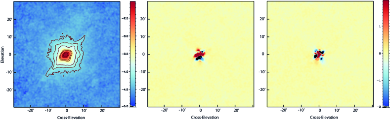
Figure 1: Total intensity $I$ (left), $Q$ (center) and $U$ (right) beam maps obtained on Jupiter during flight#3 before correction of systematic effects discussed here. The images are shown in instrument coordinates with elevation increasing upward and cross-elevation (azimuth) increasing to the right. The images are shown in arbitrary units in logarithmic scale for $I$ and linear scale for $Q$ and $U$. The elongation across the first diagonal in the total intensity image is due to cross-talk. The negative shadow of the cross-talk signal, the PSF distortion visible above the lower left-upper right diagonal and the faint residual source appearing below the planet along the other diagonal are due to read-out latency. The non-zero $Q$ and $U$ originate from intensity to polarization leakage. These effects are described in Sect. 4

Assuming a perfect HWP, the PILOT measurements $m$ are related to the input Stokes parameters $I$, $Q$, $U$ of partially linearly polarized light through

$$m=R_{xy}T_{xy}\times[I\pm Q_{inst}\cos 4\omega\pm U_{inst}\sin 4\omega]+O_{xy},$$ (1)

where $R_{xy}$ and $T_{xy}$ are the detectors response and optical transmission respectively, and $O_{xy}$ is an arbitrary electronics offset. For the configuration of the HWP and polarizer in the instrument, $\omega$ is the angle between the HWP fast axis direction and the horizontal direction measured counterclockwise as seen from the instrument. The $\pm$ sign is $+$ and $-$ for the REFLEX and TRANS arrays respectively (see Bernard_etal2016 ). Note that, with the above conventions, $Q_{inst}$ and $U_{inst}$ are defined with respect to instrument coordinates in the IAU convention, with $Q_{inst}$=0 for vertical polarization. For PILOT, $\omega$ is related to a mechanical HWP position called $HWP_{\rm pos}$, which can be varied continuously over the range 1 $\leq HWP_{\rm pos}\leq$ 8 as

$$\omega=87.25{\rm{}^{o}}-(HWP_{\rm pos}-5)\times 11.25{\rm{}^{o}},$$ (2)

allowing the HWP fast axis to vary by approx. $\pm 45{\rm{}^{o}}$ around the vertical direction. When referring to the sky polarization $Q$ and $U$, Eq. 1 becomes

$$m=R_{xy}T_{xy}\times[I\pm Q\cos(2\theta)\pm U\sin(2\theta)]+O_{xy},$$ (3)

where $\theta=2\times\omega+\phi$ is the analysis angle, $\phi$ is the time varying parallactic angle measured counterclockwise from equatorial north to Zenith for the time and direction of the current observation, and $Q$ and $U$ are in the IAU convention with respect to equatorial coordinates. In practice, maps of $Q$ and $U$ are derived from observing the same patch of sky with at least two values of the analysis angle taken at different times in general. Inversion to derive sky maps of $I$, $Q$ and $U$ can be done through polarization map-making algorithms (see for instance deGasperis+2005 ). The light polarization fraction $p$ and polarization direction $\psi$ are then defined as:

$$p=\frac{\sqrt{Q^{2}+U^{2}}}{I}$$ (4)

and

$$\psi=0.5\times\arctan(U/Q).$$ (5)

3 The PILOT flights and observations

Table 2: Observations obtained during flight#3.

Source	Observation Time [mn]	Map size [deg x deg]	Total depth [$deg^{2}/h$]
Aquila Rift	128.5	7 x 2	6.5
Crab nebula	100.	1.5 x 1.2	1.1
Fan	118.5	5 x 3.2	0.8
Jupiter	33.	2 x 1	3.6
M31	301.6	4 x 1.8	1.4
MW L133	101.58	3 x 2.8	5.0
Orion	140.1	5 x 2.5	5.3
Tau B211	50.1	2 x 1.8	4.3
Tau L1506	160	2 x 1.9	1.4
SkydipM31	20.	32 x 2	n/a
SkydipPol	33.1	44 x 2	n/a

PILOT is carried to the stratosphere by a generic gondola suspended under an open stratospheric balloon through a flight chain, with a helium gas volume of $\sim$ 800 000 m³ at ceiling altitude. The flights are operated by the French National Space Agency (CNES) with launch campaigns involving several international balloon experiments (up to six per campaign).

At ceiling altitude, the instrument can be pointed towards a given sky direction using the gondola rotation around the flight chain and rotation of the instrument around the elevation axis (see Bernard_etal2016 ). Scientific observations are organized into individual observing tiles (also called observations for short) during which a given rectangular region of the sky is scanned by combining the azimuth and elevation rotations. The flight plan is built taking into account the various observational constraints such as the visibility of astronomical sources, the minimum allowed angular distance between the instrument optical axis and bright sources such as the Sun or the Moon, elevation limits due to the presence of the Earth at low elevations and the balloon at high elevations. The expected performance of the instrument is taken into account when establishing the flight plan, in order to distribute the observing time according to the science objectives, and to evenly distribute both the polarization analysis directions (angle $\theta$ in Eq. 3) and the scanning directions for any given astronomical target.

The first two flights of the PILOT experiment took place from the launch-base facilities at the airports of Timmins (Ontario, Canada) in 2015, and Alice Springs (Australia) in 2017, respectively. A detailed description of the characteristics of these flights and the corresponding observations are presented in Mangilli2019b . In this paper, we focus on the instrument performance during the third PILOT flight.

3.1 Performance during flight#3

The third flight of the PILOT instrument took place from Timmins on September 24 2019, as part of a balloon experiment launch campaign led by CNES and the Canadian Space Agency (CSA).

The flight lasted approximately 26 hr, during which 21 hr of scientific observations were obtained. The launch took place at 5:36 AM local time. The experiment reached ceiling altitude about 2.3 hr after launch. The instrument reached an altitude of 39 km, slowly decreasing to 37 km during the first day of the flight. The altitude decreased to 34 km during the night due to the lower buoyancy force of the balloon. During the second day, the altitude rose again, reaching 37.5 km just before the gondola was dropped in Quebec. The temperatures of the focal planes evolved slightly with altitude during the ceiling period and remained in the range $296.5$ to $297$ mK and $300$ to $301$ mK for the TRANS and REFLEX focal planes respectively during the day, and $\simeq 297.5$ mK and $\simeq 301.5$ mK during the night. The higher nocturnal temperatures are due to less efficient pumping on the He bath. Out of the eight bolometer arrays, array #1 (TRANS), array #5 (TRANS) and array #6 (TRANS) were not operational during flight#3. The footprint of the available arrays on the sky is shown in Fig. 6.

The balloon followed a trajectory towards the north-east during most of the flight. We successfully used the two telemetry antennas located in Timmins and Chibougamau. The gondola was recovered about 900 km north-east of the launch site, north of Saguenay, Quebec. The gondola was brought back to the Timmins base using a helicopter and a truck. The gondola and the instrument suffered no major damage from landing or recovery, which was later confirmed by a thorough inspection following the return of the instrument to France. The astronomical sources targeted during flight#3 are listed in Table 2. In the following, we concentrate on the analysis of the data obtained on Jupiter, which we use to characterize systematic effects.

4 Systematic effects

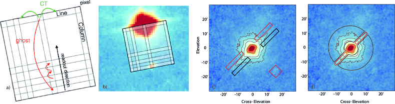
Figure 2: From left to right: (a): Schematic view of the array showing the readout direction and the effect of cross-talk along lines and read-out latency effects. (b): Image of Jupiter obtained by leaving in glitch detected samples, overlaid with the footprint of the detectors, showing the effect of the cross-talk along the lines and the presence of a ghost opposite to the planet along readout columns due to read-out latency. (c): The regions overlaid on the image of Jupiter delineate the zones used to measure the read-out latency parameters (red) and the corresponding reference regions (black). (d): The regions overlaid on the image of Jupiter delineate the zones used to measure the cross-talk effect parameters (red) and the corresponding reference regions (black).

In this section we describe three instrumental systematic effects of the PILOT data, not addressed in Mangilli2019a . Two of these effects are related to the readout electronics of the PILOT detectors, which we refer to as cross-talk and read-out latency. The third effect is produced by the optics of the instrument, which we refer to as leakage (see Sect. 4.3). Here, we describe the manifestation of each of these effects on the instrument Point Spread Function (PSF) as observed on Jupiter during flight#3, how we measured the parameters used in the correction methods, how the corrections were performed and the overall performance of the corrections, as measured on the Jupiter observations.

During each flight of the instrument, we observed planets, which can be considered point sources at the resolution of PILOT. These observations can be used to assess the optical quality through a measurement of the PSF. During Flight#3, we observed Jupiter at its maximum elevation of $\simeq 17^{\circ}\,$ during about 30 min at the start of the flight. We obtained eight individual maps using eight positions of the HWP, sampling the available analysis range uniformly. The maps were obtained at two different scanning angles to enable low frequency noise removal. The data were corrected for the responses calculated on the residual atmospheric signal and the ICS calibration signals, and corrected for the effect of the detector time constants through deconvolution, as described in Mangilli2019a . The signal was then processed using the Scanamorphos map-making software described in Roussel2013 and as used in its polarization version in Mangilli2019b to produce maps of the Stokes parameters I, Q and U and the corresponding variances and co-variances. Note that these maps can also be obtained in instrument coordinates, also referred to as cross-elevation and elevation, by setting the parallactic angle to zero in Eq. 3. This representation is optimal to reveal and characterize effects that project in the focal plane of the instrument, since it avoids blurring through sky rotation.

In order to produce PSF maps that are sufficiently accurate to be used for leakage correction, we constructed Jupiter maps with a pixel size of $6^{\prime\prime}\,$. We generated individual maps for each detector array and for each individual observation of the planet. We use these maps for assessing potential temporal or focal plane variations of the systematic effects.

Figure 1 shows the maps of Jupiter in instrumental coordinates where all the data from flight#3 have been used. Below, we use these maps to investigate systematic effects affecting the PSF in polarization, and to measure the parameters used in the correction method.

4.1 Cross-talk

Figure 1 shows the total intensity map of Jupiter obtained during flight#3 in instrument coordinates. A blurred linear extension is clearly visible across the PSF from the lower-left to upper-right of the image. As illustrated in Fig. 2, this direction corresponds to the orientation of the individual pixel lines on the arrays, which are rotated $45^{\circ}\,$ with respect to instrument coordinates. The readout electronics of the PILOT detectors is such that the signals from bolometers along each line are transferred simultaneously to a buffer unit (BU) with 16 registers for amplification. We interpret the observed effect as cross-talk between pixels along a given detector line, which could happen within the BU. As the strong signal from the peak of the optical PSF falls on a given pixel of the array, part of its intensity is transferred through cross-talk to other pixels along the corresponding detector line, producing the observed pattern. This is illustrated in Fig. 2 which shows the projection of the array footprint on the Jupiter map.

We model the cross-talk as the transfer of a fraction $f_{CT}(i,k)$ of the signal from pixel $i$ to pixel $k$ along line $j$. As the transfer is likely to occur in the buffer unit which is common to all lines, we further assume that $f_{CT}(i,k)$ is independent of line number $j$. We therefore subtract cross-talk following

$$d^{\prime}_{ij}=d_{ij}-\sum_{k\neq i}{f_{CT}(i,k)\times d_{kj}}+\sum_{k\neq i}{f_{CT}(i,k)\times d_{ij}},$$ (6)

where $d_{ij}$ and $d^{\prime}_{ij}$ are the signal before and after cross-talk subtraction respectively, and the summations are carried out over all pixels along the line under consideration. The two terms correspond to the signal received and given by the considered pixel. We also assume that, cross-talk being an induction effect, it is symmetric with $f_{CT}(i,k)$ = $f_{CT}(k,i)$.

We searched for possible variations of the cross-talk coefficient along detector lines. For this, we analyzed jointly the recordings of pixels receiving a strong glitch (normally masked out during the processing) and the stacked signal of simultaneous recordings of other pixels of the same line. We correlated the stacked signals from the main glitched pixel and the cross-talk pixel. This analysis did not produce convincing evidence for variations of $f_{CT}(i,k)$ along the pixel lines. We therefore assume that $f_{CT}(i,k)$ does not vary across a given array and we search for a single value of the pixel-to-pixel cross-talk coefficient $f_{CT}$ for each array.

In order to determine $f_{CT}$ for each array, we defined a cross-talk region and a reference region in each image of Jupiter (see Fig. 2). Both regions share the same average distance from the planet so that they would have the same brightness in the absence of cross-talk but are centered on a regions of high and low cross-talk signals respectively. The value of $f_{CT}$ for each array was found through a $\chi^{2}$ minimization of the signal difference between the cross-talk and the reference regions in images of Jupiter obtained with each array separately. At each iteration of the minimization, the cross-talk signal was subtracted from the timeline using Eq. 6 and a new image was produced. The resulting values of the cross-talk parameters $f_{CT}$ are given in Tab. 3. The derived values appear consistent between arrays and at a level just below $10^{-3}$. The values are comparable between arrays and there appear to be no particular similarities between parameter values for arrays sharing the same BU.

The Jupiter map after correction of the cross-talk using the parameters given in Tab. 3 and Eq. 6 is shown in Fig. 4.

Table 3: Cross-talk parameters derived for each array. Column 1 gives the name of the corresponding focal plane, column 2 gives the array number, column 3 gives the Buffer Unit (BU) number associated to reading the array, column 4 gives the value for the cross-talk coefficient derived.

Focal Plane	Array	BU	$f_{CT}$
TRANS	2	2	$9.0810^{-4}$
REFLEX	3	3	$8.3110^{-4}$
REFLEX	4	3	$9.0810^{-4}$
REFLEX	7	4	$9.6910^{-4}$
REFLEX	8	4	$9.3310^{-4}$

Following the correction for cross-talk, the amplitude of the effect as measured in the regions defined above is about $0.9\%$ of the PSF peak value, significantly smaller than the initial value of $4.8\%$.

4.2 Read-out latency

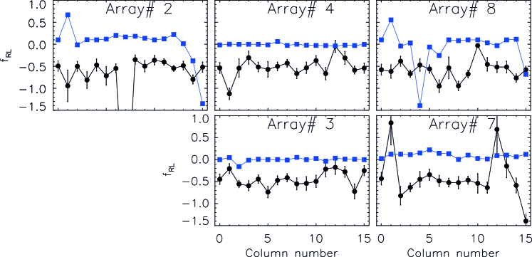
Figure 3: Parameters for the read-out latency derived for each array, plotted as a function of the readout column. The black curve shows the parameter values between adjacent pixels along the column. The blue curve shows the parameter values when readout returns from line 16 to line 1.

Figure 2 shows a map of Jupiter obtained during flight#3 where the Scanamorphos glitch detection was inhibited during processing. The map is overlaid with the footprint of one of the PILOT bolometer arrays. The image clearly shows some positive signal located precisely one array away from Jupiter along the column direction of the array. This fake source appears in the data stream of bolometers located on line 1 of each array, only when a bright source is present on the same column on line 16. This effect had already been seen clearly in calibration data, when a bright source was moved over all pixels of all arrays (Misawa_etal2017 ). It is attributed to latency in the time-multiplexed readout electronics, which we refer to as read-out latency. This effect transfers some of the signal from one readout to the next along the readout direction (see Fig. 2), including when the readout goes from line 16 back to line 1, which creates the fake positive source in the map. The effect is also seen as a negative shadow of the cross-talk signal described in Sect. 4.1, which indicates that the read-out latency effect is mostly negative during transfer across the array and positive when readout is reset to line 1. The fact that we see the effect of the read-out latency on the cross-talk signal also shows that the read-out latency happens after the cross-talk in the detection chain, and as a consequence it needs to be corrected before cross-talk in the data processing.

We model the read-out latency effect as the transfer of a fraction $f_{RL}(i,j)$ of the signal from readout $j$ to readout $j+1$ along a given column $i$. We correct for the effect in the timelines using

$$d^{\prime}_{ij}=d_{ij}-f_{RL}(i,j-1)\times d_{ij-1}+f_{RL}(i,j+1)\times d_{ij+1},$$ (7)

where all readouts have been ordered with time of acquisition. The first term corresponds to the signal received by the considered pixel from the previous readout and the second term corresponds to the signal given to the next readout. We further assume the same value for $f_{RL}(i,j)$ between all consecutive readouts, except for multiples of 16 ($j=n\times 16$) with value $f_{RL}(i,16)$ in Eq. 7. In order to measure the parameter $f_{RL}(i,j)$ for each readout column $i$ and array for $j\neq n\times 16$ , we constructed images of Jupiter in instrument coordinates using only the signal from that individual column of that individual array, using a timeline corrected according to Eq. 7. We optimized the value of $f_{RL}(i,j)$ in order to minimize the difference between the average signal in two rectangular boxes located on both sides of the cross-talk extension around Jupiter, as shown in Fig. 2. In order to measure $f_{RL}(i,16)$, we performed a similar minimization but minimizing the signal in a square box centered on the fake source in the images as shown in Fig. 2. In both cases, the minimization was performed using the $\chi^{2}$ minimization algorithm implemented in the $IDL$ routine mpfitfun.

The values derived for $f_{RL}(i,j)$ are shown in Fig. 3 for each column of each array. The values are generally negative, while $f_{RL}(i,16)$ is generally much smaller in absolute value but mostly positive.

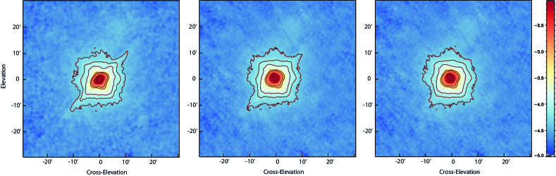
Figure 4: Images of Jupiter constructed from uncorrected data (left), corrected for read-out latency (middle), corrected for read-out latency and cross-talk (right). All images are shown in the same arbitrary units in logarithmic scale.

The Jupiter map after correction of the read-out latency using the parameters shown in Fig. 3 and Eq. 7 is shown on Fig. 4. Note that this correction produces a significant shift of the planet peak position. Since we compute sky coordinates of each data sample using the data from the Estadius stellar sensor and correcting for the offset between the sensor and the PILOT instrument optical axis using the position of observed bright sources, we recompute coordinates following that correction, which we use for the rest of the data processing and analysis.

4.3 Leakage

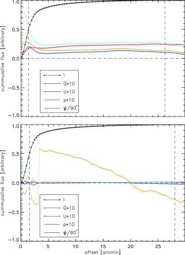
Figure 5: Cumulative intensity profiles as a function of integration radius from the peak of the total intensity in Jupiter maps. The black curve shows the cumulative profile of the total intensity. The red and dark-blue curves show the Q and U profiles multiplied by 10. The light blue and yellow curves show the corresponding average polarization leakage fraction in units of 10%, and the corresponding polarization angle divided by $90{\rm{}^{o}}$. The top panel shows the initial leakage characteristics before correction. The bottom panel shows the leakage characteristics after correction for read-out latency, cross-talk and leakage. The erratic behavior of the polarization angle on this panel is due to the very low magnitude of $Q$ and $U$ after correction.

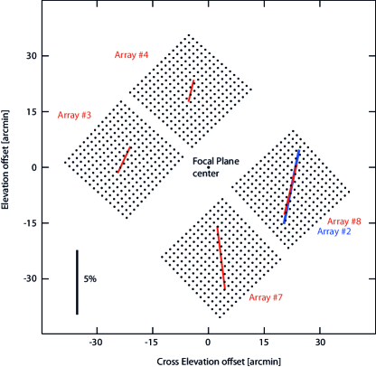
Figure 6: Distribution of the leakage polarization direction and intensity across the PILOT focal plane. The focal plane is shown in instrument coordinates, with elevation corresponding to the vertical direction, in offsets from the focal plane center. The circles show the positions of individual pixels of the TRANS arrays. The labels give the name of each operational array in red and blue for the REFLEX and TRANS focal plane respectively. The lines show the direction and amplitude of the intensity to the polarization leakage as measured on Jupiter for each array independently, in red and blue for the REFLEX and TRANS arrays respectively. The scale on the bottom left shows 5%.

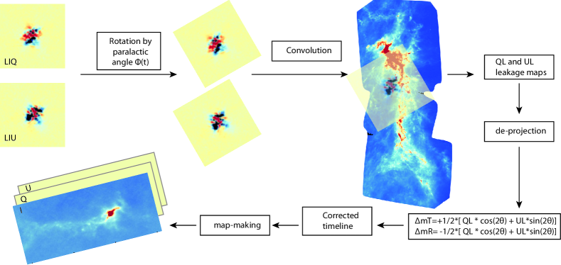
Figure 7: Schematic representation of the method used to correct for the intensity to polarization leakage in the PILOT data. The data processing steps proceed clockwise from top-left. The I, Q and U PSF as measured on Jupiter are rotated to follow the time-dependent sky rotation. They are then convolved to the high resolution Herschel satellite sky map of the considered object (here the Orion A region) at $250\,{\rm\mu m}$ sky to produce instantaneous maps of the Q and U leakage. The instantaneous maps are re-observed to produce a correction time-line which is subtracted from the original data. Our final leakage-corrected, science-ready maps are constructed by applying our map-making algorithm to this corrected timeline.

Figure 1 shows the $I$, $Q$ and $U$ maps obtained on Jupiter during flight#3 projected in instrument coordinates (elevation and cross-elevation). While we expect Jupiter to show no polarization, the maps clearly show some residual $Q$ and $U$ structures at the location of the planet.

Figure 5 shows the cumulative profiles of the $I$, $Q$ and $U$ as a function of the integration radius in the maps of Fig. 1, as well as the corresponding profiles for polarization fraction p and polarization angle $\psi$. It is clear that even when averaged over a large area, the $Q$ and $U$ cumulative profiles do not converge to zero. The corresponding values of the leakage are summarized in Table 4. Before leakage correction, the leakage polarization is of the order of p=2.4% when integrated over the whole PSF and p=4.7% when integrated over the PSF down to its FWHM. This is non-negligible compared to the typical polarization of thermal dust in the ISM, with a most likely value of around $3\%$, as measured by Planck at 353 GHz (planck2014-xix ). Given the amplitude of this leakage effect compared to the expected astrophysical signal, it clearly needs to be subtracted accurately from the data.

This effect is known as instrumental polarization and is also often referred to as leakage from total intensity to polarization. It has been observed in the polarization data of many, if not all, instruments measuring polarization. Some procedures have been proposed to subtract the effect from the data, for instruments such as NIKA2 (Ritacco2017 ), ACTPol (Guan2021 ) or HAWC+ (LopezRodriguezetal2022 ). The origin of the effect is unclear, but observations suggest that it is due to the propagation of light in the instrument.

Table 4: Leakage correction performance. Columns 1 to 3 indicate which corrections are applied. Column 4 gives the polarization fraction of the leakage as integrated over the whole PSF. Column 5 gives polarization fraction of the leakage as integrated up to the FWHM of the PSF.

RL	CT	leakage	$p_{fwhm}[\%]$	$p_{tot}[\%]$
-	-	-	5.36	2.19
x	-	-	5.38	2.62
x	x	-	4.74	2.41
x	x	x	0.17	0.28

As seen in Fig. 1, the leakage pattern of the PILOT instrument does not show any distinctive structure. This is unlike the pattern observed for the NIKA2 instrument for instance. This difference may be due to the fact that we use an off-axis telescope that has no occultation by the support for the secondary mirror. The leakage is also seen to produce mostly $U$ in instrument coordinates, which indicates that the instrumental polarization is mostly horizontal in those coordinates, corresponding to a polarization vector roughly vertical. This is compatible with the leakage being due to asymmetries in the optical system, which is mostly symmetrical with respect to the vertical direction for the PILOT instrument (see for instance Bernard_etal2016 ).

In order to investigate possible variations of the leakage with the position in the focal plane, we constructed separate maps of Jupiter with the 5 operational arrays available during flight#3. For each image, we computed the integrated leakage polarization fraction and angle integrated over the FWHM of the total intensity beam. Figure 6 shows the distribution of the polarization fraction and orientations in the PILOT focal plane. The direction is roughly vertical across the focal plane and the fraction also varies slightly. Note that the directions are consistent between arrays 2 and 8 which are optical conjugates on the sky.

4.4 Leakage correction performances

The scheme we use to subtract the leakage is illustrated in Fig. 7. We adopt the description proposed by Ritacco2017 for the NIKA2 data, in which the leakage can be computed as the convolution of the total intensity map of the sky with the leakage PSF measured on a planet. The method implemented in the PILOT pipeline involves rotating the Q and U leakage PSFs by the parallactic angle to bring them to the correct sky orientation. The rotated leakage PSF maps are then convolved with the total intensity map of the sky to produce some leakage Q and U maps. Note that this has to be done at each time sample of the time-line to account for the continuous sky rotation. The leakage Q and U maps are then interpolated at the sky coordinates corresponding to each data sample, in order to predict a leakage signal through Eq. 1. That signal is then subtracted from the original timeline and the corrected timeline is used to produce a map corrected for the leakage, using the Scanamorphos map-making algorithm. Note that, unlike in Ritacco2017 , we do not subtract any fixed polarization contribution other than the above leakage. The performances quoted therefore reflect the correction of the intensity to polarization leakage through the algorithm described here.

For the leakage PSF maps, we use the Jupiter maps shown in Fig. 1 computed in instrument coordinates and with Q and U also in reference to instrumental coordinates. As a consequence, we set the parallactic angle $\phi$ to zero in Eq. 1 when computing the leakage contribution to be subtracted from the original timeline. For the total intensity map, we use the Herschel map of the astronomical object extracted from the ESA Herschel Science Archive , which we reproject into the appropriate equatorial coordinates. This approach is preferred to deconvolving our own intensity map from our total intensity PSF, given the accuracy required for a proper subtraction of the leakage signal. In the case of Jupiter, we use a fake source map where the total intensity map of the planet is computed as a Gaussian with FWHM of $18.1^{\prime\prime}\,$, i.e. the FWHM of the $250\,{\rm\mu m}$ Herschel band. In both cases, we correlate the observed total intensity PILOT map of the object with the Herschel map and use the linear scale factor between the two images to rescale the Herschel map prior to using it to predict the leakage. In practice, the calculation of the leakage maps is performed at discrete parallactic angle values covering the range for each PILOT observation tile, with a discretization step of $\simeq 1^{\circ}\,$ and the de-projected time-lines are interpolated at the actual parallactic angle value of each data sample from those maps, using linear interpolation. The above processing is computed independently for each detector array and we use the PSF of each array as measured in maps of Jupiter computed for that array only. To first order, the processing therefore takes into account the focal-plane variations of the leakage shown in Fig. 6.

The residual polarization after leakage correction on the Jupiter data is shown in the bottom panel of Fig. 5. It can be seen that the polarization leakage is strongly reduced compared to the profiles prior to correction shown in the upper panel. The residual polarization leakage as measured at the FWHM radius of the PSF and integrated over the whole PSF are given in tab. 4 and are respectively $0.17\%$ and $0.38\%$. The spatial distribution of those residuals in the image shown on the radial profiles is likely due to uncertainties in the pointing reconstruction or in the PSF shape, discretization steps used for map rotations, etc…We also stress that a high level of accuracy must be preserved at each step of the leakage correction process, e.g. during the map rotations, convolution and timeline de-projection. Most common reprojection routines do not guarantee sufficient accuracy, and we were obliged to use drizzling methods Paradis2012 at each step. It also required working with map pixels of $6^{\prime\prime}\,$ consistent with the Herschel resolution, which are $\simeq 22$ times smaller than the PILOT beam, to produce acceptable accuracy of the correction. We note that, due to filtering of large scale emission inherent to measurements with bolometers, the leakage on extended sources should be lower than measured here on a point-like source. We consider that the range of performances given in Tab. 4 reflect those attainable on astrophysical sources with the current leakage subtraction method.

5 Conclusions

In this paper, we have presented the methods used to correct for residual systematic effects in the PILOT data, in addition to those already described in Mangilli2019a . In particular, we describe the cross-talk and read-out latency systematic effects that affect the shape of the instrument PSF in total intensity. We also described how we measure and correct for the intensity to polarization leakage and the method we use to subtract it from the data. The cross-talk and read-out latency effects are observed in the total intensity maps of Jupiter obtained during the third flight of the PILOT instrument as distortions of the instrument PSF. We measured the parameters characterizing those effects by using a simple pixel-to-pixel transfer model and derived the transfer coefficients by minimizing the PSF defects in the images of Jupiter. Our analysis showed that the read-out latency effect is observed on the cross-talk signal, indicating that it arises after cross-talk in the detection chain and therefore needs to be corrected first.

Following the above correction, images of Jupiter in polarization show polarized signal at the level of $\simeq 3\%$, which we interpret as leakage from total intensity to polarization, also known as instrumental polarization. Polarization leakage likely affects most instruments measuring polarization in the FIR/submm at a similar level. Using images of Jupiter obtained separately for the five bolometer arrays that were operational during flight#3, we showed that the leakage is mostly oriented parallel to the symmetry axis of the instrument, which points towards residual asymmetries of the optics as the origin of the leakage. We also showed that the polarization direction and fraction vary across the focal plane, an effect that we also take into account in the correction. We correct for the leakage in the PILOT pipeline following the method initially proposed by Ritacco2017 to correct for the leakage in the NIKA2 instrument. We use the I, Q and U PSFs measured on Jupiter, rotated to follow sky rotation and convolved with a scaled intensity sky map obtained by the Herschel satellite at $250\,{\rm\mu m}$ to predict maps of the leakage in sky coordinates. Those convolved leakage maps are de-projected onto the timeline of each detector to infer the correction for each detector, taking into account at first order the observed spatial variations of the leakage. We emphasize that accuracy must be preserved at each step of the process in the map rotations, convolution and timeline de-projection. This is not guaranteed by most reprojection routines. Applying our correction strategy to the Jupiter data and using a simple synthetic PSF model for the planet yields a residual polarization fraction lower than $\simeq 0.4\%$, which we regard as the accuracy of our leakage correction method.

- (1) A. Mangilli, G. Foënard, J. Aumont, A. Hughes, B. Mot, J.P. Bernard, A. Lacourt, I. Ristorcelli, L. Montier, Y. Longval, P. Ade, Y. André, L. Bautista, P. deBernardis, O. Boulade, F. Bousqet, M. Bouzit, N. Bray, V. Buttice, M. Charra, M. Chaigneau, B. Crane, E. Doumayrou, J.P. Dubois, X. Dupac, C. Engel, P. Etcheto, P. Gelot, M. Griffin, S. Grabarnik, P. Hargrave, Y. Lepennec, R. Laureijs, B. Leriche, S. Maestre, B. Maffei, J. Martignac, C. Marty, W. Marty, S. Masi, F. Mirc, R. Misawa, J.M. Nicot, J. Montel, J. Narbonne, F. Pajot, E. Pérot, G. Parot, J. Pimentao, G. Pisano, N. Ponthieu, L. Rodriguez, G. Roudil, H. Roussel, M. Salatino, G. Savini, O. Simonella, M. Saccoccio, S. Stever, P. Tapie, J. Tauber, C. Tibbs, C. Tucker, Experimental Astronomy 48(2-3), 265 (2019). DOI 10.1007/s10686-019-09648-6
- (2) K. Foyle, C.D. Wilson, E. Mentuch, G. Bendo, A. Dariush, T. Parkin, M. Pohlen, M. Sauvage, M.W.L. Smith, H. Roussel, M. Baes, M. Boquien, A. Boselli, D.L. Clements, A. Cooray, J.I. Davies, S.A. Eales, S. Madden, M.J. Page, L. Spinoglio, MNRAS421, 2917 (2012). DOI 10.1111/j.1365-2966.2012.20520.x
- (3) F. Combes, M. Boquien, C. Kramer, E.M. Xilouris, F. Bertoldi, J. Braine, C. Buchbender, D. Calzetti, P. Gratier, F. Israel, B. Koribalski, S. Lord, G. Quintana-Lacaci, M. Relaño, M. Röllig, G. Stacey, F.S. Tabatabaei, R.P.J. Tilanus, F. van der Tak, P. van der Werf, S. Verley, A&A539, A67 (2012). DOI 10.1051/0004-6361/201118282
- (4) T. Hill, P. André, D. Arzoumanian, F. Motte, V. Minier, A. Men’shchikov, P. Didelon, M. Hennemann, V. Könyves, Q. Nguyen-Luong, P. Palmeirim, N. Peretto, N. Schneider, S. Bontemps, F. Louvet, D. Elia, T. Giannini, V. Revéret, J. Le Pennec, L. Rodriguez, O. Boulade, E. Doumayrou, D. Dubreuil, P. Gallais, M. Lortholary, J. Martignac, M. Talvard, C. De Breuck, A&A548, L6 (2012). DOI 10.1051/0004-6361/201220504
- (5) F. Boulanger, A. Abergel, J.P. Bernard, W.B. Burton, F.X. Desert, D. Hartmann, G. Lagache, J.L. Puget, A&A312, 256 (1996)
- (6) A. Lazarian, J. Quant. Spec. Radiat. Transf.79, 881 (2003). DOI 10.1016/S0022-4073(02)00326-6
- (7) A. Lazarian, J. Quant. Spec. Radiat. Transf.106, 225 (2007). DOI 10.1016/j.jqsrt.2007.01.038
- (8) D.S. Mathewson, V.L. Ford, MNRAS153, 525 (1971). DOI 10.1093/mnras/153.4.525
- (9) K. Serkowski, D.S. Mathewson, V.L. Ford, ApJ196, 261 (1975). DOI 10.1086/153410
- (10) A. Benoît, Archeops Collaboration, Advances in Space Research 33, 1790 (2004). DOI 10.1016/j.asr.2003.05.021
- (11) Planck Collaboration Int. XIX, A&A576, A104 (2015). DOI 10.1051/0004-6361/201424082
- (12) Planck Collaboration Int. XXI, A&A576, A106 (2015). DOI 10.1051/0004-6361/201424087
- (13) Planck Collaboration Int. XX, A&A576, A105 (2015). DOI 10.1051/0004-6361/201424086
- (14) BICEP2 Collaboration, P.A.R. Ade, R.W. Aikin, D. Barkats, S.J. Benton, C.A. Bischoff, J.J. Bock, J.A. Brevik, I. Buder, E. Bullock, C.D. Dowell, L. Duband, J.P. Filippini, S. Fliescher, S.R. Golwala, M. Halpern, M. Hasselfield, S.R. Hildebrandt, G.C. Hilton, V.V. Hristov, K.D. Irwin, K.S. Karkare, J.P. Kaufman, B.G. Keating, S.A. Kernasovskiy, J.M. Kovac, C.L. Kuo, E.M. Leitch, M. Lueker, P. Mason, C.B. Netterfield, H.T. Nguyen, R. O’Brient, R.W. Ogburn, A. Orlando, C. Pryke, C.D. Reintsema, S. Richter, R. Schwarz, C.D. Sheehy, Z.K. Staniszewski, R.V. Sudiwala, G.P. Teply, J.E. Tolan, A.D. Turner, A.G. Vieregg, C.L. Wong, K.W. Yoon, Physical Review Letters 112(24), 241101 (2014). DOI 10.1103/PhysRevLett.112.241101
- (15) D.A. Harper, M.C. Runyan, C.D. Dowell, C.J. Wirth, M. Amato, T. Ames, M. Amiri, S. Banks, A. Bartels, D.J. Benford, M. Berthoud, E. Buchanan, S. Casey, N.L. Chapman, D.T. Chuss, B. Cook, R. Derro, J.L. Dotson, R. Evans, D. Fixsen, I. Gatley, J.A. Guerra, M. Halpern, R.T. Hamilton, L.A. Hamlin, C.J. Hansen, S. Heimsath, A. Hermida, G.C. Hilton, R. Hirsch, M.I. Hollister, C.F. Hostetter, K. Irwin, C.A. Jhabvala, M. Jhabvala, J. Kastner, A. Kovács, S. Lin, R.F. Loewenstein, L.W. Looney, E. Lopez-Rodriguez, S.F. Maher, J.M. Michail, T.M. Miller, S.H. Moseley, G. Novak, R.J. Pernic, T. Rennick, H. Rhody, E. Sandberg, D. Sandford, F.P. Santos, R. Shafer, E.H. Sharp, P. Shirron, J. Siah, R. Silverberg, L.M. Sparr, R. Spotz, J.G. Staguhn, A.S. Toorian, S. Towey, J. Tuttle, J. Vaillancourt, G. Voellmer, C.G. Volpert, S.I. Wang, E.J. Wollack, Journal of Astronomical Instrumentation 7(4), 1840008-1025 (2018). DOI 10.1142/S2251171718400081
- (16) W.S. Holland, D. Bintley, E.L. Chapin, A. Chrysostomou, G.R. Davis, J.T. Dempsey, W.D. Duncan, M. Fich, P. Friberg, M. Halpern, K.D. Irwin, T. Jenness, B.D. Kelly, M.J. MacIntosh, E.I. Robson, D. Scott, P.A.R. Ade, E. Atad-Ettedgui, D.S. Berry, S.C. Craig, X. Gao, A.G. Gibb, G.C. Hilton, M.I. Hollister, J.B. Kycia, D.W. Lunney, H. McGregor, D. Montgomery, W. Parkes, R.P.J. Tilanus, J.N. Ullom, C.A. Walther, A.J. Walton, A.L. Woodcraft, M. Amiri, D. Atkinson, B. Burger, T. Chuter, I.M. Coulson, W.B. Doriese, C. Dunare, F. Economou, M.D. Niemack, H.A.L. Parsons, C.D. Reintsema, B. Sibthorpe, I. Smail, R. Sudiwala, H.S. Thomas, MNRAS430(4), 2513 (2013). DOI 10.1093/mnras/sts612
- (17) M. Calvo, A. Benoît, A. Catalano, J. Goupy, A. Monfardini, N. Ponthieu, E. Barria, G. Bres, M. Grollier, G. Garde, J.P. Leggeri, G. Pont, S. Triqueneaux, R. Adam, O. Bourrion, J.F. Macías-Pérez, M. Rebolo, A. Ritacco, J.P. Scordilis, D. Tourres, A. Adane, G. Coiffard, S. Leclercq, F.X. Désert, S. Doyle, P. Mauskopf, C. Tucker, P. Ade, P. André, A. Beelen, B. Belier, A. Bideaud, N. Billot, B. Comis, A. D’Addabbo, C. Kramer, J. Martino, F. Mayet, F. Pajot, E. Pascale, L. Perotto, V. Revéret, A. Ritacco, L. Rodriguez, G. Savini, K. Schuster, A. Sievers, R. Zylka, Journal of Low Temperature Physics 184(3-4), 816 (2016). DOI 10.1007/s10909-016-1582-0
- (18) C.L.H. Hull, P.C. Cortes, V.J.M.L. Gouellec, J.M. Girart, H. Nagai, K. Nakanishi, S. Kameno, E.B. Fomalont, C.L. Brogan, G.A. Moellenbrock, R. Paladino, E. Villard, PASP132(1015), 094501 (2020). DOI 10.1088/1538-3873/ab99cd
- (19) L.M. Fissel, P.A.R. Ade, F.E. Angilè, S.J. Benton, E.L. Chapin, M.J. Devlin, N.N. Gandilo, J.O. Gundersen, P.C. Hargrave, D.H. Hughes, J. Klein, A.L. Korotkov, G. Marsden, T.G. Matthews, L. Moncelsi, T.K. Mroczkowski, C.B. Netterfield, G. Novak, L. Olmi, E. Pascale, G. Savini, D. Scott, J.A. Shariff, J.D. Soler, N.E. Thomas, M.D.P. Truch, C.E. Tucker, G.S. Tucker, D. Ward-Thompson, D.V. Wiebe, in Millimeter, Submillimeter, and Far-Infrared Detectors and Instrumentation for Astronomy V, Proc. SPIE, vol. 7741 (2010), Proc. SPIE, vol. 7741, pp. 77,410E–77,410E–14. DOI 10.1117/12.857601
- (20) V. Guillet, L. Fanciullo, L. Verstraete, F. Boulanger, A.P. Jones, M.A. Miville-Deschênes, N. Ysard, F. Levrier, M. Alves, A&A610, A16 (2018). DOI 10.1051/0004-6361/201630271
- (21) Planck Collaboration Int. XXII, A&A, submitted 576, A107 (2015). DOI 10.1051/0004-6361/201424088
- (22) P.C.M.P.C. XIII, A&A571, A13 (2014). DOI 10.1051/0004-6361/201321553
- (23) Planck Collaboration, N. Aghanim, Y. Akrami, M. Ashdown, J. Aumont, C. Baccigalupi, M. Ballardini, A.J. Banday, R.B. Barreiro, N. Bartolo, S. Basak, K. Benabed, J.P. Bernard, M. Bersanelli, P. Bielewicz, J.R. Bond, J. Borrill, F.R. Bouchet, F. Boulanger, M. Bucher, C. Burigana, E. Calabrese, J.F. Cardoso, J. Carron, A. Challinor, H.C. Chiang, L.P.L. Colombo, C. Combet, F. Couchot, B.P. Crill, F. Cuttaia, P. de Bernardis, A. de Rosa, G. de Zotti, J. Delabrouille, J.M. Delouis, E. Di Valentino, J.M. Diego, O. Doré, M. Douspis, A. Ducout, X. Dupac, G. Efstathiou, F. Elsner, T.A. Enßlin, H.K. Eriksen, E. Falgarone, Y. Fantaye, F. Finelli, M. Frailis, A.A. Fraisse, E. Franceschi, A. Frolov, S. Galeotta, S. Galli, K. Ganga, R.T. Génova-Santos, M. Gerbino, T. Ghosh, J. González-Nuevo, K.M. Górski, S. Gratton, A. Gruppuso, J.E. Gudmundsson, W. Handley, F.K. Hansen, S. Henrot-Versillé, D. Herranz, E. Hivon, Z. Huang, A.H. Jaffe, W.C. Jones, A. Karakci, E. Keihänen, R. Keskitalo, K. Kiiveri, J. Kim, T.S. Kisner, N. Krachmalnicoff, M. Kunz, H. Kurki-Suonio, G. Lagache, J.M. Lamarre, A. Lasenby, M. Lattanzi, C.R. Lawrence, F. Levrier, M. Liguori, P.B. Lilje, V. Lindholm, M. López-Caniego, Y.Z. Ma, J.F. Macías-Pérez, G. Maggio, D. Maino, N. Mandolesi, A. Mangilli, P.G. Martin, E. Martínez-González, S. Matarrese, N. Mauri, J.D. McEwen, A. Melchiorri, A. Mennella, M. Migliaccio, M.A. Miville-Deschênes, D. Molinari, A. Moneti, L. Montier, G. Morgante, A. Moss, S. Mottet, P. Natoli, L. Pagano, D. Paoletti, B. Partridge, G. Patanchon, L. Patrizii, O. Perdereau, F. Perrotta, V. Pettorino, F. Piacentini, J.L. Puget, J.P. Rachen, M. Reinecke, M. Remazeilles, A. Renzi, G. Rocha, G. Roudier, L. Salvati, M. Sandri, M. Savelainen, D. Scott, C. Sirignano, G. Sirri, L.D. Spencer, R. Sunyaev, A.S. Suur-Uski, J.A. Tauber, D. Tavagnacco, M. Tenti, L. Toffolatti, M. Tomasi, M. Tristram, T. Trombetti, J. Valiviita, F. Vansyngel, B. Van Tent, L. Vibert, P. Vielva, F. Villa, N. Vittorio, B.D. Wandelt, I.K. Wehus, A. Zonca, A&A641, A3 (2020). DOI 10.1051/0004-6361/201832909
- (24) R. Banerji, G. Patanchon, J. Delabrouille, M. Hazumi, D. Thuong Hoang, H. Ishino, T. Matsumura, J. Cosmology Astropart. Phys.2019(7), 043 (2019). DOI 10.1088/1475-7516/2019/07/043
- (25) M. Lopez-Radcenco, J.M. Delouis, L. Vibert, A&A651, A65 (2021). DOI 10.1051/0004-6361/202040152
- (26) P. Friberg, D. Berry, G. Savini, D. Bintley, J. Dempsey, S. Graves, H. Parsons, in Millimeter, Submillimeter, and Far-Infrared Detectors and Instrumentation for Astronomy IX, Society of Photo-Optical Instrumentation Engineers (SPIE) Conference Series, vol. 10708, ed. by J. Zmuidzinas, J.R. Gao (2018), Society of Photo-Optical Instrumentation Engineers (SPIE) Conference Series, vol. 10708, p. 107083M. DOI 10.1117/12.2314345
- (27) A. Ritacco, N. Ponthieu, A. Catalano, R. Adam, P. Ade, P. André, A. Beelen, A. Benoît, A. Bideaud, N. Billot, O. Bourrion, M. Calvo, G. Coiffard, B. Comis, F.X. Désert, S. Doyle, J. Goupy, C. Kramer, S. Leclercq, J.F. Macías-Pérez, P. Mauskopf, A. Maury, F. Mayet, A. Monfardini, F. Pajot, E. Pascale, L. Perotto, G. Pisano, M. Rebolo-Iglesias, V. Revéret, L. Rodriguez, C. Romero, F. Ruppin, G. Savini, K. Schuster, A. Sievers, C. Thum, S. Triqueneaux, C. Tucker, R. Zylka, A&A599, A34 (2017). DOI 10.1051/0004-6361/201629666
- (28) H. Ajeddig, R. Adam, P. Ade, P. André, A. Andrianasolo, H. Aussel, A. Beelen, A. Benoît, A. Bideaud, O. Bourrion, M. Calvo, A. Catalano, B. Comis, M. De Petris, F.X. Désert, S. Doyle, E.F.C. Driessen, A. Gomez, J. Goupy, F. Kéruzoré, C. Kramer, B. Ladjelate, G. Lagache, S. Leclercq, J.F. Lestrade, J.F. Macías-Pérez, A. Maury, P. Mauskopf, F. Mayet, A. Monfardini, L. Perotto, G. Pisano, N. Ponthieu, V. Revéret, A. Ritacco, C. Romero, H. Roussel, F. Ruppin, K. Schuster, Y. Shimajiri, S. Shu, A. Sievers, C. Tucker, R. Zylka, in European Physical Journal Web of Conferences, European Physical Journal Web of Conferences, vol. 228 (2020), European Physical Journal Web of Conferences, vol. 228, p. 00002. DOI 10.1051/epjconf/202022800002
- (29) H. Ajeddig, R. Adam, P. Ade, P. André, E. Artis, H. Aussel, A. Beelen, A. Benoît, S. Berta, L. Bing, O. Bourrion, M. Calvo, A. Catalano, M. De Petris, F.X. Désert, S. Doyle, E.F.C. Driessen, A. Gomez, J. Goupy, F. Kéruzoré, C. Kramer, B. Ladjelate, G. Lagache, S. Leclercq, J.F. Lestrade, J.F. Macías-Pérez, A. Maury, P. Mauskopf, F. Mayet, A. Monfardini, M. Muñoz-Echeverría, L. Perotto, G. Pisano, N. Ponthieu, V. Revéret, A.J. Rigby, A. Ritacco, C. Romero, H. Roussel, F. Ruppin, K. Schuster, S. Shu, A. Sievers, C. Tucker, R. Zylka, Y. Shimajiri, in European Physical Journal Web of Conferences, European Physical Journal Web of Conferences, vol. 257 (2022), European Physical Journal Web of Conferences, vol. 257, p. 00002. DOI 10.1051/epjconf/202225700002
- (30) E.E. Lopez-Rodriguez, et al., ApJ(2022 in prep.)
- (31) J.P. Bernard, the PILOT team, Experimental Astronomy 42, 199 (2016). DOI 10.1007/s10686-016-9506-1
- (32) C. Engel, I. Ristorcelli, J.P. Bernard, Y. Longval, C. Marty, B. Mot, G. Otrio, G. Roudil, Experimental Astronomy 36, 21 (2013). DOI 10.1007/s10686-013-9332-7
- (33) J. Montel, Y. Andre, F. Mirc, P. Etcheto, J. Evrard, N. Bray, M. Saccoccio, L. Tomasini, E. Perot, in 22nd ESA Symposium on European Rocket and Balloon Programmes and Related Research, ESA Special Publication, vol. 730, ed. by L. Ouwehand (2015), ESA Special Publication, vol. 730, p. 509
- (34) P. Hargrave, T. Waskett, T. Lim, B. Swinyard, in Society of Photo-Optical Instrumentation Engineers (SPIE) Conference Series, vol. 6275 (2006), p. 627514
- (35) P.C. Hargrave, J.W. Beeman, P.A. Collins, I. Didschuns, M.J. Griffin, B. Kiernan, G. Pisano, in IR Space Telescopes and Instruments, vol. 4850 (2003), Proc. SPIE, pp. 638–649
- (36) G. de Gasperis, A. Balbi, P. Cabella, P. Natoli, N. Vittorio, A&A436, 1159 (2005). DOI 10.1051/0004-6361:20042512
- (37) A. Mangilli, J. Aumont, J.P. Bernard, A. Buzzelli, G. de Gasperis, J.B. Durrive, K. Ferriere, G. Foënard, A. Hughes, A. Lacourt, R. Misawa, L. Montier, B. Mot, I. Ristorcelli, H. Roussel, P. Ade, D. Alina, P. de Bernardis, E. de Gouveia Dal Pino, J.P. Dubois, C. Engel, V. Guillet, P. Hargrave, R. Laureijs, Y. Longval, B. Maffei, A.M. Magalhaes, C. Marty, S. Masi, J. Montel, F. Pajot, E. Pérot, L. Rodriguez, M. Salatino, M. Saccoccio, G. Savini, S. Stever, J. Tauber, C. Tibbs, C. Tucker, A&A630, A74 (2019). DOI 10.1051/0004-6361/201935072
- (38) H. Roussel, PASP125, 1126 (2013). DOI 10.1086/673310
- (39) R. Misawa, the PILOT team, Experimental Astronomy 43, 211 (2017). DOI 10.1007/s10686-017-9528-3
- (40) Y. Guan, S.E. Clark, B.S. Hensley, P.A. Gallardo, S. Naess, C.J. Duell, S. Aiola, Z. Atkins, E. Calabrese, S.K. Choi, N.F. Cothard, M. Devlin, A.J. Duivenvoorden, J. Dunkley, R. Dünner, S. Ferraro, M. Hasselfield, J.P. Hughes, B.J. Koopman, A.B. Kosowsky, M.S. Madhavacheril, J. McMahon, F. Nati, M.D. Niemack, L.A. Page, M. Salatino, E. Schaan, N. Sehgal, C. Sifón, S. Staggs, E.M. Vavagiakis, E.J. Wollack, Z. Xu, ApJ920(1), 6 (2021). DOI 10.3847/1538-4357/ac133f
- (41) D. Paradis, K. Dobashi, T. Shimoikura, A. Kawamura, T. Onishi, Y. Fukui, J.P. Bernard, A&A543, A103 (2012). DOI 10.1051/0004-6361/201118740