Determination of class-specific variables in nonparametric multiple-class classification

Wan-Ping Nicole Chen

Institute of Statistical Science

Academia Sinica

Taipei, Taiwan 11529

wpchen@stat.sinica.edu.tw

Yuan-chin Ivan Chang

Institute of Statistical Science

Academia Sinica

Taipei, Taiwan 11529

ycchang@stat.sinica.edu.tw

Key Words: multiple-class, multi-class classification, nonparametric classification, kernel density estimation, sparsity, bandwidth selection

ABSTRACT As technology advanced, collecting data via automatic collection devices become popular, thus we commonly face data sets with lengthy variables, especially when these data sets are collected without specific research goals beforehand. It has been pointed out in the literature that the difficulty of high-dimensional classification problems is intrinsically caused by too many noise variables useless for reducing classification error, which offer less benefits for decision-making, and increase complexity, and confusion in model-interpretation. A good variable selection strategy is therefore a must for using such kinds of data well; especially when we expect to use their results for the succeeding applications/studies, where the model-interpretation ability is essential. hus, the conventional classification measures, such as accuracy, sensitivity, precision, cannot be the only performance tasks. In this paper, we propose a probability-based nonparametric multiple-class classification method, and integrate it with the ability of identifying high impact variables for individual class such that we can have more information about its classification rule and the character of each class as well. The proposed method can have its prediction power approximately equal to that of the Bayes rule, and still retains the ability of “model-interpretation.” We report the asymptotic properties of the proposed method, and use both synthesized and real data sets to illustrate its properties under different classification situations. We also separately discuss the variable identification, and training sample size determination, and summarize those procedures as algorithms such that users can easily implement them with different computing languages.

1 Introduction

In multiple-class classification problems, the relative position among classes can be very complicated within the variable-space, the situation becomes worse for data sets with lengthy variables. Modern machine learning methods commonly outperform the conventional statistical classification models in these situations. These methods, such as the support vector machine (SVM), may have good prediction power; however, the classification rules of them are difficult to be explained. There are also some methods build multiple-class classification rules baed on the divide-and-conquer concept via a bunch of binary classifiers, and thus rely on certain voting schemes, which make model-interpretation more difficult (see also Tomczak and Zieba, 2015). Some hybrid methods, which depend on voting-like schemes, such as random forest methods, will also suffer from model-interpretation difficulty. These nonparametric types of methods are preferred due to their flexibility, especially for problems with complicated data, such as image, and sound, where conventional parametric models are inferior. However, their classification rules are less informative for the follow-up applications/studies, where the further details of classification rules, or “model interpretation” property is essential in addition to the conventional performance measures such as accuracy, precision, and so on. Thus, the interpretation ability of classifiers catches a lot of attention (Yang et al., 2010), and also motivates this study.

For conventional classifier construction processes, when a data set has a large number of variables, we aim to find a short set of informative variables to build “separating” boundaries among classes for the ease of classification rules interpretation. This task is crucial even in binary classification problems (see Liu et al., 2008; Mechbal et al., 2015; Zhang, 2017), and it becomes more difficult to achieve in multiple-class classification problems due to the complications among classes. Moreover, if all the conditional probabilities, given each class label, of a sample are known, we can assign this sample to the class where its largest conditional probability. This classification rule is called the Bayes rule, which has the smallest error rate (see Van Ryzin, 1966). In Van Ryzin (1966), he also showed that if we accurately estimate each class density, then the classification error rate approaches to that of the Bayes rule. Since then, the probability-based classification rules have been extensively discussed in the literature (Devroye and Wagner, 1976; Greblicki and Pawlak, 1983; Har-Peled et al., 2002; George and Langley, 1995). Although there are many different probability-based methods reported, the model interpretation ability is usually out of their scopes (Ancukiewicz, 1998; Hall and Kang, 2005; Lugosi and Nobel, 1996; Kobos and Mandziuk, 2011; Yang, 1999). However, to find only one variable set for all classes in a multiple-class classification problem makes the estimation of the density of each class very difficult, since all classes have their own characters, and may not be described via the same set of variables. Thus, how to retain prediction power, while to identify proper variables of each class for improving the model-interpretation ability for multiple-class classifiers is our goal in this paper.

Shao et al. (2011) and many other researchers have pointed out that a classification rule could do as bad as random guessing without considering the sparsity condition, and complex structure in high-dimensional data sets. Fan and Fan (2008) state that the difficulty of high-dimensional classification problems is intrinsically caused by too many noise variables useless for reducing classification error, which offer less benefits for decision-making, and increase complexity, and confusion in model-interpretation. Moreover, they also pointed out that the “important variables” for estimating the conditional densities for individual classes can be different, and this fact makes the model-interpretation of the probability-based methods even more difficult for multiple-class classification problems. Thus, identifying the individual high impact variable set of each class plays a crucial role in both classification performance, and model-interpretation, especially when the follow-up research requires the details of the classification rules instead of just the predicted labels.

We study multiple-class classification problems under sparsity condition, where each sample belongs to only one class. Our goal is to assign new sample to the most appropriate class, and learn about “why this sample should be assigned to a particular class” through the identified variable sets of individual classes. As mentioned in Fan and Fan (2008), the selected variable sets for individual classes are not necessarily the same, thus we study the method that can identify variable sets for individual classes. We propose a variable detection process that can separately identify variable sets for estimating the density of individual classes, and then integrate such a novel variable detection procedure into a nonparametric posterior kernel density classifier approach based on a density estimation method (Sugiyama, 2010; Sugiyama et al., 2012). We call the proposed classifier NPKDC-vd, which is the short for “nonparametric posterior kernel density classifier with variable detection.”

In the rest of this paper, we discuss the theoretical properties of the proposed method, and show that this method can asymptotically reach the Bayes rule. Moreover, we describe its related algorithms including construction of classification rules, variable identification, and training sample size determination. We explain how a general probability-based-model works in Section 2.1. We also explain how we can just use the relevant variables for this task, and how to determine the number of relevant variables in Section 2.2. In Section 2.3, we introduce the hypotheses testing ignorer to take the estimation variance into our procedure. Then, in Section 2.4, we explain how we can decide the training sample sizes of each class. The asymptotic property of the proposed method is in Section 2.5, and its proof is in the Supplementary. We then illustrate our method with numerical studies with the synthesized and real data in Section 3 and 4, respectively, and then summarize our findings in the Summary section.

2 Nonparametric Posterior Kernel Density Classifier with Variable Detection

2.1 Nonparametric classifier

We now describe the NPKDC-vd below. Let $\mathbf{X}\subset\mathbb{R}^{d}$ be a $d$-dimensional vector of variables, and $Y\in\{1,2,\dots,c\}$ be the class label, where $c$ is the number of classes. Suppose that we do not have any prior prevalence information of each class; i.e. assume that $P(y=Y)=1/c$, for $Y\in\{1,2,\dots,c\}$. Assume that $\mathbf{X}\times Y$ have a joint probability density function $f_{\mathbf{X},Y}(\mathbf{x},y)$, and $\mathbf{x}\in\mathbf{X}$ has a marginal density $f_{\mathbf{X}}(\mathbf{x})$, then the class-posterior probability is $P(Y=y|\mathbf{X}=\mathbf{x})={f_{\mathbf{X},Y}(\mathbf{x},y)}/{f_{\mathbf{X}}(\mathbf{x})}$. It implies that a sample $\mathbf{x}$ belong to Class ${y}$ with probability $P(Y=y|\mathbf{X}=\mathbf{x})$, and a probability-based classification rule will assign it to Class $\hat{y}$, if $\hat{y}:=\operatorname*{argmax}_{y\in\{1,\dots,c\}}P(Y=y|\mathbf{X}=\mathbf{x})$. To apply this idea we need to estimate the class-posterior probabilities, which is a challenging problem from both computational and theoretical perspectives; especially when the number of class $c$ and/or the dimension $d$ is large.

Suppose that $\{\mathbf{x}_{i},y_{i})$, $i=1,\dots,n\}$, are i.i.d paired samples of size $n$. Using the idea of the least-squares probabilistic classifier (LSPC) with a nonparametric kernel density estimation of conditional probabilities (see Sugiyama, 2010; Sugiyama et al., 2012), we have the class-posterior probability of Class $y$ as a summation of kernel bases $K^{\prime}$:

$$P(Y=y|\mathbf{X}=\mathbf{x};\bm{\alpha})=\sum_{y^{\prime}=1}^{c}\sum_{i=1}^{n}\alpha_{i}^{y^{\prime}}K^{\prime}(\mathbf{x},\mathbf{x}_{i},y,y^{\prime}),$$ (1)

which has $c\times n$ parameters: $\bm{\alpha}=(\alpha_{1}^{1},\dots,\alpha_{n}^{1},\dots,\alpha_{1}^{c},\dots,\alpha_{n}^{c})^{T}$. Let $\{\mathbf{x}_{i}^{y},i=1,\dots,n_{y}\}$ denote the samples in Class $y$ of size $n_{y}$. Then via the delta kernel for $Y$ to separate $\mathbf{X}$ and $Y$, and a symmetric Gaussian kernel $\mathcal{K}$ on samples within the target class to reduce the number of kernels, we have the class-posterior probability for Class $y$ as follows:

$$P(Y=y|\mathbf{X}=\mathbf{x};\bm{\beta^{y}}):=\sum_{i=1}^{n_{y}}\beta_{i}^{y}\mathcal{K}(\mathbf{x},\mathbf{x}_{i}^{y}),$$ (2)

where $\beta^{y}$, $y=1,\ldots,c$, is an unknown vector to be estimated. Assume $\beta^{y}$, $y=1,\ldots,c$, are known, then assign sample $\mathbf{x}$ to Class $\hat{y}$, if

$$\hat{y} :=\operatorname*{argmax}_{y\in\{1,\dots,c\}}P(Y=y|\mathbf{X}=\mathbf{x};\bm{\beta^{y}}):=\operatorname*{argmax}_{y\in\{1,\dots,c\}}\sum_{i=1}^{n_{y}}\beta_{i}^{y}\mathcal{K}(\mathbf{x},\mathbf{x}_{i}^{y}).$$

Note that (2) suggests that we can decompose the original problem into $c$ independent problems, and use only the training samples of each class to estimate its own posterior probability. Because we do not use the whole training samples for an individual class, the number of parameters is equal to $\sum_{y=1}^{c}n_{y}$ parameters, which is smaller than that in (1). Thus, using this decomposition can cut down the computational cost. Moreover, via such decomposition, we can carry out this learning process with a parallel computing facility, or a machine with multi-core/multi-thread CPUs; that is, we can learn $c$ models simultaneously and separately.

2.2 Bandwidth determination

The conventional LSPC uses a prefixed bandwidth for its Gaussian kernels for each class. This setting is not suitable when the density of each class has its own key variables, which is common in multiple-class classification problems (see also Fan and Fan, 2008).

We propose a bandwidth selection process and integrate it into (2) such that the estimates via (2) can have different smoothing parameters for individual coordinates of its kernel density estimation. Then the class-posterior density becomes

$$P(Y=y|\mathbf{X}=\mathbf{x};H_{y}) :=\frac{1}{n_{y}}\sum_{i=1}^{n_{y}}\frac{1}{\det(H_{y})}\mathcal{K}(H_{y}^{-1}(\mathbf{x}-\mathbf{x}_{i}^{y}))$$

$$:=\frac{1}{n_{y}}\sum_{i=1}^{n_{y}}\prod_{j=1}^{d}\frac{1}{h_{j}^{y}}K\Big{(}\frac{x_{j}-x_{ij}^{y}}{h_{j}^{y}}\Big{)},$$ (3)

where $H_{y}=diag(h_{1}^{y},\dots,h_{d}^{y})$ is a diagonal matrix and its element $h_{j}^{y}$ is the bandwidth of one-dimensional Gaussian kernel $K$ in the $j$th coordinate for Class $y$. From (3), if ${h_{j}^{y}}$ is small, then its correspondent variable will have larger contributions to the posterior density. For a probability-based classification rule, the samples in Class $y$ should have higher class-posterior probability for Class $y$. It follows that variables with smaller bandwidth values (i.e. $h_{j}^{y}$’s in (3)) are more important to the posterior density of Class $y$. Then the classification rule of NPKDC-vd via (3) becomes

$$\hat{y}=\operatorname*{argmax}_{y\in\{1,\dots,c\}}\frac{1}{n_{y}}\sum_{i=1}^{n_{y}}\prod_{j=1}^{d}\frac{1}{h_{j}^{y}}K\Big{(}\frac{x_{j}-x_{ij}^{y}}{h_{j}^{y}}\Big{)}.$$ (4)

We then treat the bandwidths as some unknown parameters to be estimated with data, and will discuss its estimation procedure below.

2.2.1 Greedy bandwidth estimation

Scott and Sain (2005) claim that the direct estimation of the full density by kernel methods is only feasible when the dimension of variable vector is no larger than 6. There are many criteria reported in the literature for determining bandwidth. However, as far as we know, most of them consider all variables equally and ignore the effects of the variables with no or little impact (Leiva-Murillo and Artés-Rodríguez, 2012; Gu et al., 2013), such that their methods suffer from the curse of dimensionality due to too many redundant variables included in the estimating processes (see also Fan and Fan, 2008). The computational cost is one of the major issues for deciding the bandwidth for each dimension of data sets with lengthy variables. Thus, identifying high impact variable sets efficiently and effectively for density estimation of each class will not only largely improve the interpretation ability and classification performance, but reduce the computational cost. Here we combine the idea of LSPC, and the regularization of derivative expectation operator (rodeo) (see Liu et al., 2007) together in the proposed bandwidth selection procedure such that we can detect the relevant variables with faster convergence rate and lower computational cost.

Without loss of generality and for simplicity of discussion, we rearrange the order of variables in each Class $y$, $y=1,\ldots,c$, such that the first $r_{y}$ variables, $X_{j}:j=1\leqslant j\leqslant r_{y}$, are relevant high impact variables for the given class, and $X_{j}:j=r_{y}+1\leqslant j\leqslant d$ are the rest irrelevant ones. (Please note that this arrangement is only for the convenience of discussion, and is not necessary in practice.) Let $R_{y}=\{j:1\leqslant j\leqslant r_{y}\}$ and $R_{y}^{c}=\{j:r_{y}+1\leqslant j\leqslant d\}$ be two index sets, where $r_{y}$ is the number of the relevant variables for Class $y$, $y=1,\ldots,c$, and this number can be different among classes. The details about determining the largest $r_{y}$ for the index set $R_{y}$ are in Section 2.3, and Algorithm 1 is for this purpose.

We may omit the subscript $y$ of $R_{y}$ and $r_{y}$ from our formulas in the following discussion when there is no ambiguity. Assume, for the moment, that $r_{y}=r$ is the largest number of key variables for class density estimation, and the rest variables have little or no impact, then the posterior density function of Class $y$ can be rewritten as

$$P\big{(}Y=y|\mathbf{X}=\mathbf{x};H_{y}\big{)} =g_{Y|\mathbf{X}_{R}}\big{(}\mathbf{x}_{R};H_{y}^{R}\big{)}u(\mathbf{x}_{R^{c}})=g_{Y|\mathbf{X}_{R}}(\mathbf{x}_{R},H_{y}^{R}),$$

where $u(\cdot)$ is a uniform function, $g_{Y|\mathbf{X}_{R}}$ depends only on the set $\mathbf{X}_{R}$, and $H_{y}^{R}=diag(h_{1}^{y},\dots,h_{r}^{y})$ is an $r\times r$ submatrix of $H_{y}$. Then (3) becomes

$$P\big{(}Y=y|\mathbf{X}=\mathbf{x};H_{y}\big{)}=\frac{1}{n_{y}}\sum_{i=1}^{n_{y}}\prod_{j=1}^{d}\frac{1}{h_{j}^{y}}K\Big{(}\frac{x_{j}-x_{ij}^{y}}{h_{j}^{y}}\Big{)}$$

$$=\frac{1}{n_{y}}\sum_{i=1}^{n_{y}}\left[\prod_{j=1}^{r}\frac{1}{h_{j}^{y}}K\Big{(}\frac{x_{j}-x_{ij}^{y}}{h_{j}^{y}}\Big{)}\right]\left[\prod_{j=r+1}^{d}\frac{1}{h_{j}^{y}}K\Big{(}\frac{x_{j}-x_{ij}^{y}}{h_{j}^{y}}\Big{)}\right]$$ (5)

$$\approx\frac{1}{n_{y}}\sum_{i=1}^{n_{y}}\left[\prod_{j=1}^{r}\frac{1}{h_{j}^{y}}K\Big{(}\frac{x_{j}-x_{ij}^{y}}{h_{j}^{y}}\Big{)}\right].$$ (6)

The second term of (5) follows a uniform distribution by assumption. Hence, we can use a large bandwidth value on $h_{j},j=r+1,\dots,d$, as in the greedily bandwidth selection approach, to get a smooth kernel density function to estimate such a uniform function. Thus, we can use (6) to approximate (5).

Let $\mathbf{x}=(x_{i},\dots,x_{d})^{T}$ be a sample of Class $y$. Using (6), the estimated posterior density of $\mathbf{x}$ is

$$P\big{(}Y=y|\mathbf{X}=\mathbf{x};H_{y}\big{)}=\frac{1}{n_{y}}\sum_{i=1}^{n_{y}}\prod_{j=1}^{d}\frac{1}{h_{j}^{y}}K\Big{(}\frac{x_{j}-x_{ij}^{y}}{h_{j}^{y}}\Big{)}.$$

To determine bandwidths, we start with a bandwidth matrix $H_{y}=\textit{diag}(h_{0},\dots,h_{0})$ with a large $h_{0}$ via the rodeo method, and compute derivatives, for $1\leqslant j\leqslant d$,

$$Z_{j} =\frac{\partial P\big{(}Y=y|\mathbf{X}=\mathbf{x};H_{y}\big{)}}{\partial h_{j}^{y}}=\frac{1}{n_{y}}\sum_{i=1}^{n_{y}}\frac{\partial}{\partial h_{j}^{y}}\left[\prod_{k=1}^{d}\frac{1}{h_{k}^{y}}K\Big{(}\frac{x_{k}-x_{ik}}{h_{k}^{y}}\Big{)}\right]$$

$$\equiv\frac{1}{n_{y}}\sum_{i=1}^{n_{y}}Z_{ji}.$$ (7)

If $K$ is the Gaussian kernel, then $Z_{j}$ becomes

$$Z_{j} =\frac{1}{n_{y}}\sum_{i=1}^{n_{y}}Z_{ji}=\frac{1}{n_{y}}\sum_{i=1}^{n_{y}}\frac{(x_{j}-x_{ij})^{2}-(h_{j}^{y})^{2}}{(h_{j}^{y})^{3}}\prod_{k=1}^{d}\frac{1}{h_{k}^{y}}K\Big{(}\frac{x_{k}-x_{ik}}{h_{k}^{y}}\Big{)}.$$ (8)

If the derivative $|Z_{j}|$ is small and the corresponding value of $h_{j}^{y}$ is relatively large, it suggests that the variable $X_{j}$ may be irrelevant in the current density estimation. If $|Z_{j}|$ is large and to change $h_{j}^{y}$ will lead to a substantial change in its corresponding estimate, then we set the bandwidth equal to a smaller number $\gamma\times h_{j}^{y}$, where $\gamma\in(0,1)$ is a small constant. We repeat this procedure for each $j$, $j=1,\ldots,d$, and keep shrinking its corresponding bandwidth in discrete steps, such as $1,\gamma,\gamma^{2},\dots$, until the value of $|Z_{j}|$ is less than a given threshold $\lambda_{j}$.

To take the estimation variance into consideration, we use the sample variance of $Z_{j}$s, say $s_{j}^{2}$, to estimate $\sigma_{j}^{2}\equiv\mbox{Var}(Z_{j})$. Following the suggestion of Liu et al. (2007) and to balance variance against bias, we set a threshold $\lambda_{j}=s_{j}\sqrt{2\log(n_{y}c)}$ with $c=O(\log n_{y})$. Once we have the posterior densities for all classes, we use (4) as a rule to assign a class label for each sample. Algorithm 3 describes how to estimate the posterior density estimate with bandwidth selection for each class. (Note that users can use other kernel functions with these algorithms via some modifications.)

2.3 Variable identification and training sample size determination

We use the estimated bandwidths obtained from Algorithm 3 as indices of the relevant level of variables, which depends on the estimate of posterior density of each class, and therefore can be different among classes. This novel variable determination method for constructing multiple-class classifiers can greatly improve the model-interpretation ability of classification rules, and provide more information applications or planning further studies.

Identifying high impact variables

We have the local bandwidths $\hat{h}_{j,i}^{y}$ of each variable $X_{j}$, $j=1,\dots,d$, in each Class $y$ after applying Algorithm 3 to the training samples of each class. As discussed before, if $X_{j}$ is a relevant variable, then it should have a smaller bandwidth compared with that of irrelevant variables in this class. Because estimates of bandwidths depend on the samples, we take the variances of bandwidth estimates into consideration via adopting statistical hypotheses testing procedures to decide whether there are significant differences among the bandwidths of variables. We state this procedure below:

Step 1: We first want to know whether all bandwidth means are equal, so the null and alternative hypotheses are

$$H_{0}:~{} \bar{h}_{1}^{y}=\bar{h}_{2}^{y}=\dots=\bar{h}_{d}^{y}$$ (9)

$$H_{1}:~{} \text{not all bandwidth means are equal},$$

where $\bar{h}_{j}^{y}=\sum_{i=1}^{n_{y}}\hat{h}_{j,i}^{y}/n_{y}$, $j=1,\dots,d$. In our algorithm, all bandwidths start from the same initial value $h_{0}$. We use a one-way analysis of variance (ANOVA), and reject the null hypothesis if

$$F\equiv MS_{B}/MS_{w}>F_{\alpha,d-1,n_{y}\cdot d-d},$$ (10)

where $MS_{B}$ is between-class mean square, $MS_{w}$ is within-class mean square, and $F_{\alpha,d-1,n_{y}\cdot d-d}$ is the upper $100\cdot(1-\alpha)$th percentile of the F distribution with parameters $d-1$ and $n_{y}\cdot d-d$ degree of freedom.

Step 2. Rejecting the null hypothesis in (9) indicates that all bandwidth means are not the same. We then want to make sure which means are different via a post-hoc analysis through a multiple pairwise comparison:

$$H_{0}:~{} \bar{h}_{m}^{y}=\bar{h}_{n}^{y},~{}~{}m,n=1,~{}\dots,d,m\neq n$$ (11)

$$H_{1}:~{} \bar{h}_{m}^{y}\neq\bar{h}_{n}^{y}.$$

Because multiple testings are performed together, we adopt Tukey’s honestly significant difference (Tukey’s HSD) procedure, instead of $t$-test, based on the studentized range distribution (Hochberg and Tamhane, 1987; Tukey, 1949). Thus, the null hypothesis in (11) is rejected if

$$|t_{mn}|=\frac{|\bar{h}_{m}^{y}-\bar{h}_{n}^{y}|}{\sqrt{MS_{w}(\frac{2}{n_{y}})}}>\frac{1}{\sqrt{2}}q_{\alpha,d,n_{y}\cdot d-d},$$ (12)

where $q_{\alpha,d,n_{y}\cdot d-d}$ is the upper $100(1-\alpha)$th percentile of the studentized range distribution with parameters $d$ and $n_{y}\cdot d-d$ degree of freedom. To identify relevant variables, we need to know exactly which variables have the bandwidth means which are significantly smaller than others, To accelerate the testing process, we arrange the bandwidth means in an increasing order. Denote the sorted bandwidth means as $\bar{h}_{1^{*}}^{y}\leq\bar{h}_{2^{*}}^{y}\leq\dots\leq\bar{h}_{d^{*}}^{y}$, then we aim to find

$$o=\operatorname*{argmax}_{m=1,\dots,d}\Big{\{}|t_{m^{*}n^{*}}|=\frac{|\bar{h}_{m^{*}}^{y}-\bar{h}_{n^{*}}^{y}|}{\sqrt{MSE(\frac{2}{n_{y}})}}>\frac{1}{\sqrt{2}}q_{\alpha,d,n_{y}\cdot d-d},\forall~{}n>m\Big{\}}.$$ (13)

Because after sorting, bandwidths $\bar{h}_{m^{*}}^{y},~{}m<o$ is smaller than $\bar{h}_{o^{*}}$, they are all significantly smaller than $\bar{h}_{n^{*}},\forall n>o$. It implies that the corresponding $\bar{h}_{o^{*}}$ is significantly smaller than $\bar{h}_{n^{*}},\forall n>o$. Thus, we choose the corresponding variables $X_{1^{*}},\dots,X_{o^{*}}$ as the relevant variables in Class $y$ as follows:

$$j\in\begin{cases}R_{y},&\text{if }\ \bar{h}_{j}^{y}\leqslant\bar{h}_{o^{*}}^{y}\\ R_{y}^{c},&\text{otherwise}.\end{cases}$$ (14)

We summarize this variable selection procedure as Algorithm 1. For convenience, we also put the classification and this class-specific variable determination together as Algorithm 2.

The proposed approach emphasizes more on “understanding how each sample is assigned to a class,” or “these samples belong to a particular class due to which variables.” This is, of course, different from the conventional model interpretation of linear or other parametric models. However, this information is useful in some research/decision-making scenarios, such as medical/pharmaceutical studies, manufacturing, and so on. Note that these algorithms are easily implemented with multi-core/multi-thread computers, or parallel computing facilities. Thus, they will not dramatically increase the computational cost.

Data:

• $\mathbf{x}_{i}=(x_{i1},\dots,x_{id})^{T},i=1,\dots,n_{y}$: training data set of Class $y$

Input:

• $\alpha$: significant level

Output:

• High impact index set $R_{y}$

Learning

1. for $i=1,\dots,n_{y}$ do

       Find the local bandwidths $\hat{H}_{y,i}=\text{diag}(\hat{h}_{1,i}^{y},\dots,\hat{h}_{d,i}^{y})$ for data point $\mathbf{x}_{i}$ by Algorithm 3

end for

Calculate bandwidth means $\bar{h}_{j}^{y}$, $j=1,\dots,d$. 3. one-way ANOVA test for equality of all bandwidth means by (9) and (10) 4. Stop if null hypothesis (9) is not rejected, otherwise continue 5. Tukey’s HSD for Post-Hoc Analysis by (11) and (12) 6. Find the largest mean $\bar{h}_{o*}^{y}$ that has significant different than all the larger ones by (13) 7. Decide $R^{y}$ by (14).

Algorithm 1 Variable Selection for Individual Classes

Data: $\{\mathbf{x}^{y^{\prime}}\}=\{\mathbf{x}^{y^{\prime}}_{1},\dots,\mathbf{x}^{y^{\prime}}_{n_{y^{\prime}}}\}$, ${y^{\prime}}=1,\dots,c$: training data set in $y^{\prime}$th class;

             $\{\mathbf{x}_{i},y_{i}\}$ : $i=1,\dots,m$ : testing data

Input: $0<\gamma<1$: reduce rate for bandwidth,

             $h_{0}=c_{0}/\log\log n$: initial bandwidth,

             $\tau$: threshold

Output: Estimated label: $\hat{y}_{i}$, $i=1,\dots,m$,

                Selected variables: $R^{y^{\prime}}$, $y^{\prime}=1,\dots,c$

Learning

for $y^{\prime}=1,\dots,c$ do

       Use training data set $\{\mathbf{x}^{y^{\prime}}\}$

       for $i=1,\dots,m$ do

            

            Estimate bandwidths $\hat{H}_{y^{\prime},i}=(\hat{h}^{y^{\prime}}_{i1},\dots,\hat{h}^{y^{\prime}}_{id})$ via Algorithm 3 on testing data $\mathbf{x}_{i}$.

             Calculate the estimated density $\hat{p}(y=y^{\prime}|\mathbf{x}_{i};\hat{H}_{y^{\prime},i})$

       end for

      

end for

Classification

$\hat{y}_{i}=\operatorname*{argmax}_{y^{\prime}}\frac{\hat{p}(y=y^{\prime}|\mathbf{x}_{i};\hat{H}_{y^{\prime},i})}{\sum_{y^{\prime}=1}^{c}\hat{p}(y^{\prime}|\mathbf{x}_{i};\hat{H}_{y^{\prime},i})}$, $i=1,\dots,m$

Accuracy $=\{\sum_{i=1}^{m}I(\hat{y}_{i}=y_{i})\}/m$, where $I(\cdot)$ is an indicator function.

Variable Selection

for $y^{\prime}=1,\dots,c$ do

       ($\hat{h}^{y^{\prime}}_{1},\dots,\hat{h}^{y^{\prime}}_{d})=\frac{\sum_{i=1}^{m}H_{y^{\prime},i}\times I(\hat{y}_{i}=y^{\prime})}{\sum_{i=1}^{m}I(\hat{y}_{i}=y^{\prime})}$

       Apply Variable Selection algorithm for Class $y^{\prime}$ and get $R_{y^{\prime}}$

end for

Algorithm 2 Integration of Classification and Variable Detection

2.4 Training Sample Sizes of Individual classes

In general, when training sample sizes among classes are highly imbalanced, we will usually obtain a biased classification rule with this training set. On the other hand, a class with more relevant variables requires larger training sample size to estimate its density in our approach. To use an equal sample size for all classes is a simple, but inefficient, approach. Thus, different classes require different training sample sizes, and to have appropriate training sample sizes among classes is important for multiple-class classification problems. To this end, we propose a two-step method for estimating the “optimal” sample sizes of individual classes based on Theorem 2.1, when a pilot study is allowed. We summarize the procedure as Algorithm LABEL:alg4 in Supplementary, for calculating training samples sizes.

Let $K$ be a $d$-dimensional bounded symmetric kernel (see also (LABEL:eq:kernel)) satisfying

$$\int K(u)du=1_{d},\text{ and }\int uK(u)du=0_{d},$$ (15)

and let $\nu$ and $\kappa$ be

$$\nu=\int_{\mathbb{R}^{d}}uu^{T}K(u)du,\text{ and }\kappa=\Big{(}\int_{\mathbb{R}^{d}}K^{2}(u)du\Big{)}^{1/2}.$$ (16)

Suppose that there is a set of initial samples for all individual classes, then by Theorem 2.1 (see also (LABEL:eq:errorrate3)), we have

$$L_{n}-L^{\star} \leqslant\sum_{y^{\prime}=1}^{c}\Bigg{(}\hat{p}_{y^{\prime}}\int\Big{|}f_{y^{\prime}}(\mathbf{x})-\hat{f}_{y^{\prime}}(\mathbf{x})\Big{|}dx+\int f_{y^{\prime}}(\mathbf{x})\Big{|}p_{y^{\prime}}-\hat{p}_{y^{\prime}}\Big{|}dx\Bigg{)}$$

$$=\sum_{y^{\prime}=1}^{c}\Bigg{(}\mathcal{O}\Big{(}n_{y^{\prime}}^{-2/(4+r_{y^{\prime}})}\Big{)}+\mathcal{O}\Big{(}\sqrt{\log(\log(n))/n}\Big{)}\Bigg{)}.$$

It follows that the convergence rate of $L_{n}-L^{\star}$ is asymptotically dominated by

$$\sum_{y^{\prime}=1}^{c}\hat{p}_{y^{\prime}}\int\Big{|}f_{y^{\prime}}(\mathbf{x})-\hat{f}_{y^{\prime}}(\mathbf{x})\Big{|}dx.$$ (17)

Thus, for a given $\epsilon>0$, we have

$$\sum_{y^{\prime}=1}^{c}\frac{n_{y^{\prime}}}{n}\Bigg{(}\frac{\nu}{2}\int\Big{|}\sum_{j=1}^{r_{y^{\prime}}}k_{j}^{y^{\prime}2}f_{y^{\prime}}^{(jj)}\Big{|}+\kappa\Big{(}\prod_{j=1}^{r_{y^{\prime}}}k_{j}^{y^{\prime}}\Big{)}^{-1/2}\int\sqrt{f_{y^{\prime}}}\Bigg{)}n_{y^{\prime}}^{-\frac{2}{4+r_{y^{\prime}}}}\leqslant\epsilon.$$ (18)

Equation (18) implies that

$$\sum_{y^{\prime}=1}^{c}n_{y^{\prime}}^{\frac{2+r_{y^{\prime}}}{4+r_{y^{\prime}}}}\Bigg{(}\frac{\nu}{2}\int\Big{|}\sum_{j=1}^{r_{y^{\prime}}}k_{j}^{y^{\prime}2}f_{y^{\prime}}^{(jj)}\Big{|}+\kappa\Big{(}\prod_{j=1}^{r_{y^{\prime}}}k_{j}^{y^{\prime}}\Big{)}^{-1/2}\int\sqrt{f_{y^{\prime}}}\Bigg{)}\leqslant n\epsilon.$$ (19)

Let $\vec{A}=(A_{1},\dots,A_{c})^{\prime}$, and $\vec{B}=(B_{1},\dots,B_{c})^{\prime}$ be the vectors with components

$$A_{y^{\prime}}= n_{y^{\prime}}^{(2+r_{y^{\prime}})/(4+r_{y^{\prime}})},\text{ and }$$ (20)

$$B_{y^{\prime}}= \frac{\nu}{2}\int\Big{|}\sum_{j=1}^{r_{y^{\prime}}}k_{j}^{y^{\prime}2}f_{y^{\prime}}^{(jj)}\Big{|}+\kappa\Big{(}\prod_{j=1}^{r_{y^{\prime}}}k_{j}^{y^{\prime}}\Big{)}^{-1/2}\int\sqrt{f_{y^{\prime}}},\;\;y^{\prime}=1\dots,c,$$ (21)

respectively. Then, $\sum_{y^{\prime}=1}^{c}A_{y^{\prime}}B_{y^{\prime}}=\vec{A}\cdot\vec{B}\leqslant n\epsilon$ suffices to guarantee that $\eqref{eq:samplesize2}\leqslant n\epsilon$. This inner product $\vec{A}\cdot\vec{B}$ reaches its maximum, when $\vec{A}$ and $\vec{B}$ are parallel. Hence, for a given $\epsilon>0$, if individual sample sizes satisfying $A\propto B$ with the total sample size equal to $n$, then the difference of error rates between the proposed procedure and Bayes rule is approximately less than $\epsilon$. Since the true density functions are unknown, we use the estimated density functions instead. Then, via Monte-Carlo integral method, we have the components of vectors $\vec{A}$ and $\vec{B}$ as follows:

$$\hat{A}_{y^{\prime}}= n_{y^{\prime}}^{(2+\hat{r}_{y^{\prime}})/(4+\hat{r}_{y^{\prime}})}$$ (22)

$$\hat{B}_{y^{\prime}}= \frac{\nu}{2}\sum_{\{\mathbf{x}^{\hat{y}^{\prime}}\}}\frac{\Big{|}\sum_{j=1}^{\hat{r}_{y^{\prime}}}k_{j}^{y^{\prime}2}\hat{f}_{y^{\prime}}^{(jj)}(\mathbf{x})\Big{|}}{\hat{f}_{y^{\prime}}(\mathbf{x})}+\kappa\Big{(}\prod_{j=1}^{\hat{r}_{y^{\prime}}}k_{j}^{y^{\prime}}\Big{)}^{-1/2}\sum_{\{\mathbf{x}^{\hat{y}^{\prime}}\}}\frac{\sqrt{\hat{f}_{y^{\prime}}(\mathbf{x})}}{\hat{f}_{y^{\prime}}(\mathbf{x})}.$$ (23)

Thus, with a given error bound, a pre-decided total sample size, and the information obtained from the first stage, we can adopt a two-stage procedure to estimate the required sample size of each class.

Algorithm LABEL:alg4 in Supplementary (see Section LABEL:ss) describes a two-stage approach based on the above discussion, which includes two steps: estimation and resampling. From the estimation step (E-step), we have the estimated bandwidths for each class, and the estimated labels of samples. Using the estimated density and predicted label, we then use the formula above to decide whether to include more training samples in the resampling step (R-step), for the given error bound $\epsilon$ and total sample size $n$. Because the precision of the estimated sample sizes depends on the initial samples of individual classes, a reasonable size of initial samples for each class is required.

2.5 Asymptotic properties and Algorithm of classification rule

Let $\hat{f}_{y^{\prime}}(\mathbf{x};\hat{H}_{y^{\prime}})$ be the estimated probability density function using rodeo method with the estimated bandwidth matrix $\hat{H}_{y^{\prime}}=diag(\hat{h}_{1}^{y^{\prime}},\dots,\hat{h}_{d}^{y^{\prime}})$. Then we have the following theorem, and the proof of it is in Supplementary LABEL:Proof_of_Theorem_1.

Theorem 2.1.

Assume the sample size in Class $y^{\prime}$ is $n_{y^{\prime}}$, and the total sample size is equal to $n=\sum_{y^{\prime}\in\mathcal{Y}}n_{y^{\prime}}$. Let $\hat{p}_{y^{\prime}}=n_{y^{\prime}}/n$ be the sample proportion, and $\hat{f}_{y^{\prime}}(\mathbf{x};\hat{H}_{y^{\prime}})$ be the estimates via rodeo methiod. Then the classification rule:

$$\hat{y}=\operatorname*{argmax}_{y^{\prime}\in\mathcal{Y}}\hat{p}_{y^{\prime}}\hat{f}_{y^{\prime}}(\mathbf{x};\hat{H}_{y^{\prime}})$$ (24)

approximates to the Bayes rule:

$$y=\operatorname*{argmax}_{y^{\prime}\in\mathcal{Y}}p_{y^{\prime}}f_{y^{\prime}}(\mathbf{x}).$$ (25)

Let $L^{\star}$ and $L_{n}$ denote the probability of error rates of (25) (the Bayes rule), and (24), respectively. Then $L_{n}-L^{*}\rightarrow 0$ with probability one, as $\min_{y^{\prime}=1,\ldots,c}\{n_{y^{\prime}}\}$ goes to $\infty$.

Algorithm 3 describes the steps for conducting the NPKDC-vd – short for the nonparametric posterior kernel density classifier with the proposed bandwidth selection procedure.

Data:

• $\mathbf{x}_{i}=(x_{i1},\dots,x_{id})^{T}$, $i=1,\dots,n_{y}$: training data set of Class $y$

• $\mathbf{x}$: a point on which we want to find the posterior density estimator

Input:

• $0<\gamma<1$: reduce rate for bandwidth

• $h_{0}=c_{0}/\log\log n_{y}$: initial bandwidth for some constant $c_{0}$

• $c_{n}=O(\log n_{y})$

Output:

• Bandwidths $\hat{H}_{y}=\text{diag}(\hat{h}_{1}^{y},\dots,\hat{h}_{d}^{y})$

• Posterior density estimator: $\hat{P}\big{(}Y=y|\mathbf{X}=\mathbf{x};\hat{H}_{y}\big{)}$

Initialization

$h_{j}^{y}=h_{0}$, $j=1,\dots,d$

$\mathcal{A}=\{1,2,\dots,d\}$

while $\mathcal{A}$ is nonempty do

       for $j\in\mathcal{A}$ do

             Estimate the derivative $Z_{j}$ and sample variance $s_{j}^{2}$.

             Compute the threshold $\lambda_{j}=s_{j}\sqrt{2\log(n_{y}c_{n})}$.

             If $|Z_{j}|>\lambda_{j}$, set $h_{j}^{y}\leftarrow\gamma h_{j}^{y}$; otherwise remove $j$ from $\mathcal{A}$.

       end for

      Calculate the estimated posterior probability with the estimated $\hat{H}_{y}:\hat{p}(Y=y|x,\hat{H}_{y})$

end while

Algorithm 3 Nonparametric Posterior Kernel Density Classifier with Variable Detection

3 Numerical Results: Synthesized Data

We use both synthetic and real datasets for illustration, and evaluate the performance based on both prediction power and variable detection ability. We set $c_{0}=10$, $c_{n}=\log n_{y}$, and $\gamma=0.9$ as the default parameters for our algorithms, and also used the default parameter of Gaussian kernel ion Matlab. The baselines for comparison are the results obtained from classifiers without variable detection. To have a thorough assessment, we also use different numbers of classes, allocations among classes, and different training sample sizes of each class in the numerical studies. We also apply the method of support vector machine (SVM) to the same data sets for comparison purposes. We train a SVM based multiple-class classifier via the multiple-class error-correcting output codes (ECOC) model Bagheri, Montazer, and Escalera (2012); Berger (1999), which is trained with a bunch of the SVM-based binary classifiers with standardized predictors and Gaussian kernel function (with parameter equal to 1), and assign the testing data to class with the highest class posterior probabilities. To illustrate the variable selection power of the proposed method and for comparison purposes, we adopt the method of “SVM with sequential variable selection” (SVMfs), where variables are sequentially added to train a classification rule until there is no improvement in prediction (see Bagheri, Montazer, and Escalera, 2012; Berger, 1999, for further details). SVMfs will only determine a subset, and the selected subset is shared with all classes, while our method allows each class to have its own subset of variables.

3.1 Ten-class Example

We generate a 10-class data set with 30 variables in this synthesized data set, and among them, each class has its own 6 relevant variables, which are not all the same among classes. The relevant variables in the $y$th class are: $\{y,y+1,\dots,y+5\}$, which are generated with distributions

$$X_{i}^{y}\sim\mathcal{N}(0.5,(0.02*(i-y+1))^{2}),\,\text{for }i=y:y+5,\,y=1:10,$$

and the rest irrelevant variables are generated from

$$X_{i}^{y}\sim\text{Uniform}(0,1),\,\text{for }i\in\{1:30\}\setminus\{y:y+5\},\,y=1:10.$$

The relevant variables of Class 1 are Variables 1 to 6, Class 2 has Variable 2 to 7 as its relevant variables, and so on. That is, there are only some overlapping relevant variables among nearby classes. The training and testing sample sizes for each class are 150 and 100, respectively. We repeat this study 1000 times and Table 1 shows the results based on 1000 trials. We found that when the data set has some irrelevant variables, the proposed NPKDC-vd method has better classification accuracy ($67.52\%$) compared with that of the conventional LSPC ($21.43\%$) at a price of computational time. The average computational time of NPKDC-vd is around 100 seconds, SVMfs use around 140 seconds, while LSPC, and SVM just take a few seconds. The sequential variable selection of SVMfs is based on an iterative algorithm, and that is the reason why it takes so much time. SVMfs perform better than SVM due to its variable selection procedure. The proposed NPKDC-vd method has the highest accuracy in this example, which is much better than that of SVMfs. As mentioned before, these SVM based methods rely on a bunch of SVM based binary classifiers. Thus, it is difficult to “explain” their classification rules.

Figure 1 shows the box-plots of the mean predicted bandwidths using the training samples in each class based on 1000 replications. In this plot, we can see that the mean bandwidths of the relevant variables are much smaller than those of the irrelevant ones, and the relevant variables for each class are separately identified. Table 2 summaries the probabilities of relevant variables identified via hypotheses testing described in Algorithm 1. We highlight those relevant variables of each class with gray background color in this table, and the probabilities in those gray cells are all equal to 1, and the rest are equal to 0. Hence, the NPKDC-vd can identify the relevant variables precisely – both false positive or false negative rates are 0. It also confirms the predicted bandwidth is good guidance for identifying relevant variables. Table 3 is the variable identification probability of SVMfs. We can see that the detection probability is much lower than that of NPKDC-vd. Moreover, SVMfs only selects a set of variables for all classes, while NPKDC-vd can identify the relevant variables for each class with probability 1. Thus, the NPKDC-vd method provides more precise information about each class. Moreover, we can see from this table that the computation of the posterior probability estimation with rodeo method via decomposition mentioned before, the increase in computational time is feasible (see NPKDC-vd and SVMfs in Table 1). In fact, it can be shortened further with a parallel/distributed computation framework, since those estimates can be conducted separately.

Table 1: Classification results and computation time used in Example 1

	Method
	NPKDC-vd	LSPC
Accuracy	0.6752( 0.0167)	0.2143( 0.0138)
Time/sec	101.8789( 1.5503)	2.3559( 0.0540)

	Method
	SVM	SVM(with fs)
Accuracy	0.1361( 0.0141)	0.4655( 0.0690)
Time/sec	3.7740( 0.1224)	138.4383( 26.0866)

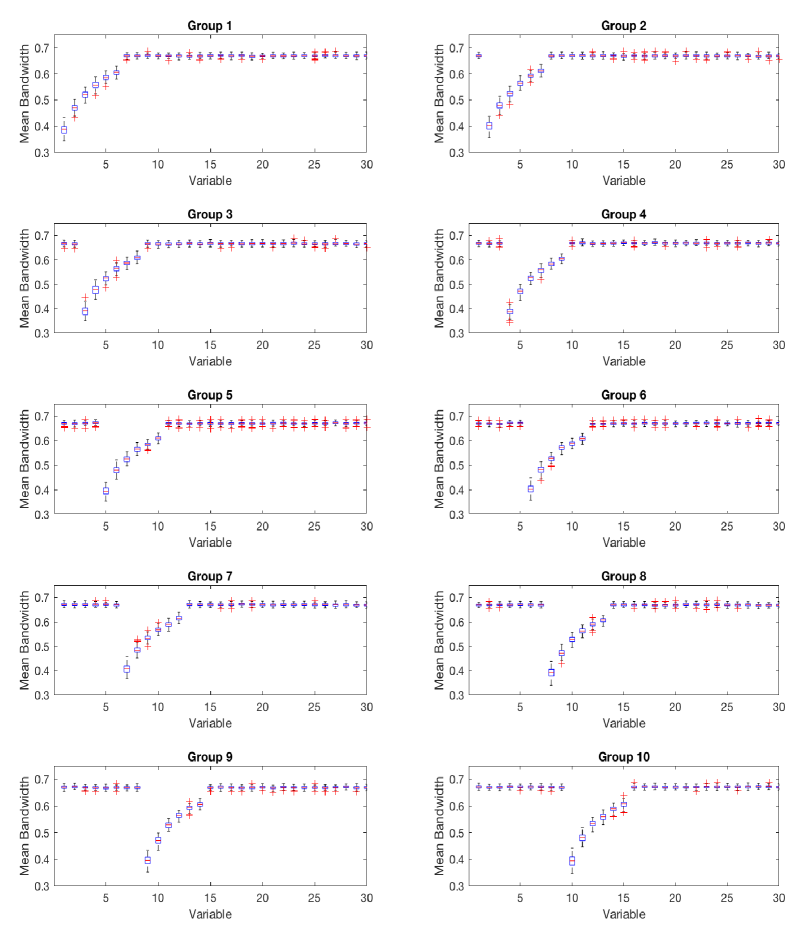
Figure 1: The box-plots of mean predicted bandwidths for the 10-class example.

Table 2: The probabilities of relevant variables identified via NPKDC-vd for Example 1 based on 1000 iterations.

	1	2	3	4	5	6	7	8	9	10
1$\sim$10	0.1100	0.2000	0.2200	0.2900	0.3900	0.5000	0.4900	0.4100	0.4400	0.3400
	11	12	13	14	15	16	17	18	19	20
1$\sim$10	0.2700	0.1300	0.0900	0.0300	0.0100	0.0000	0.0000	0.0000	0.0000	0.0000
	21	22	23	24	25	26	27	28	29	30
1$\sim$10	0.0000	0.0000	0.0000	0.0000	0.0000	0.0000	0.0000	0.0000	0.0000	0.0000

Table 3: The probabilities of relevant variables identified by SVM with sequential variable selection based on 1000 iterations, for data in Example 1.

	1	2	3	4	5	6	7	8	9	10
1$\sim$10	0.1100	0.2000	0.2200	0.2900	0.3900	0.5000	0.4900	0.4100	0.4400	0.3400
	11	12	13	14	15	16	17	18	19	20
1$\sim$10	0.2700	0.1300	0.0900	0.0300	0.0100	0.0000	0.0000	0.0000	0.0000	0.0000
	21	22	23	24	25	26	27	28	29	30
1$\sim$10	0.0000	0.0000	0.0000	0.0000	0.0000	0.0000	0.0000	0.0000	0.0000	0.0000

3.2 Asymmetric Centers of Classes

We now study the case with a complicated relative positions among classes. To illustrate this situation, we generate a 5-class data set with 10 variables, and only the first two variables are relevant in all classes. We generate 8 irrelevant variables from a uniform distribution, and the other two relevant variables from (26) below:

$$N\bigg{(}\begin{bmatrix}\mu^{y}_{1}\\ \mu^{y}_{2}\end{bmatrix},\begin{bmatrix}0.1^{2}&0\\ 0&0.2^{2}\end{bmatrix}\bigg{)},y=1:5,$$ (26)

where $\mu^{y}_{1}$ and $\mu^{y}_{2}$ are location parameters. Figure 2 shows the values of the class means in the space spanned by these two relevant variables. It shows that Class 1 (i.e. $y=1$) is surrounded by the other 4 classes in this space with different distances between their means.

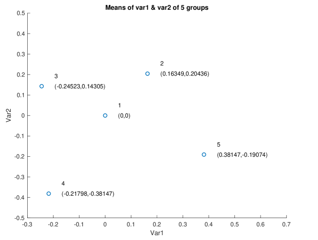
Figure 2: The means of 5 classes with asymmetric positions the first and second variables.

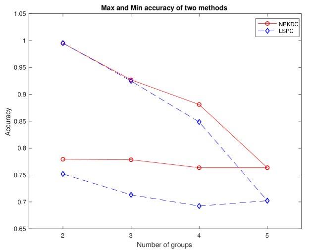
Figure 3: The maximum and minimum accuracies of two methods based on the data with asymmetric positions among classes.

We conduct studies with different combinations of these 5 classes to see how the number of classes, and their relative positions affect classification performance. The training and testing data sizes of each class are 150 and 100, respectively. Table 4 reports the classification accuracy based on 1000 replications of each study. We can see that the classification performance declines for all 4 methods when the number of classes increases, since when the number of classes increases, the relations among classes are getting complicated such that the decision boundaries among classes are vague. From this table, we can also see that the performances are not all the same among the studies with the same number of classes, which is due to the relative positions among classes being all different. We can find a similar situation in Table 5, which shows that the classification accuracy of SVM and SVMfs declines for all 4 methods when the number of classes increases. Comparing these two tables, we found that SVMfs has the highest accuracy. NPKDC-vd has slightly lower accuracy than that of SVMfs In general, methods with variable selection perform better than their own counterparts.

Table 6(b) shows the variable detection probabilities, and the probabilities of correctly selecting the first two relevant are equal to 1 for both NPKDC-vd and SVMfs. (Note that the results for other cases are similar, and therefore are omitted.) However, the false positive probabilities of NPKDC-vd are less than $1\%$, while SVMfs has falsely selected probabilities of irrelevant variables larger than $10\%$ in all multiple-class setups in this example. These results show that using estimated bandwidths for variable selection is promising. It confirms that NPKDC-vd can retain both satisfactory classification accuracy, and reveal the information of relevant variables of individual classes, which improves the interpretation ability of the corresponding classification rules.

Figure 3 is a plot of the maximum and minimum accuracies of NPKDC-vd and LSPC, which shows that NPKDC-vd has higher accuracy than that of LSPC for all cases in this example. The maximum accuracy declines as the number of classes increases for both methods . However, the minimum accuracy of NPKDC-vd retains at the level of accuracy (around 0.77) as the number of classes increases, while that of LSPC drops from 0.75 to 0.70.

Table 4: Classification accuracy on different combinations of classes in example with special located between classes in Section 3.2. The training size = 150, and testing size = 100 in each class. Results are based on 1000 repeated trials.

# of classes	2		# of classes	3
	NPKDC-vd	LSPC		NPKDC-vd	LSPC
1 2	0.7793( 0.0287)	0.7520( 0.0291)	1 2 3	0.7784( 0.0232)	0.7225( 0.0264)
1 3	0.8813( 0.0245)	0.8315( 0.0300)	1 2 4	0.7847( 0.0229)	0.7132( 0.0259)
1 4	0.9004( 0.0211)	0.8876( 0.0218)	1 2 5	0.7898( 0.0246)	0.7602( 0.0244)
1 5	0.9613( 0.0150)	0.9431( 0.0185)	1 3 4	0.8232( 0.0207)	0.7993( 0.0229)
2 3	0.9676( 0.0118)	0.9605( 0.0133)	1 3 5	0.8945( 0.0174)	0.7804( 0.0278)
2 4	0.9877( 0.0079)	0.9720( 0.0131)	1 4 5	0.9095( 0.0166)	0.8672( 0.0177)
2 5	0.9023( 0.0244)	0.8817( 0.0225)	2 3 4	0.9074( 0.0163)	0.9002( 0.0158)
3 4	0.8997( 0.0209)	0.9070( 0.0209)	2 3 5	0.9130( 0.0160)	0.8570( 0.0194)
3 5	0.9950( 0.0046)	0.9953( 0.0043)	2 4 5	0.9270( 0.0138)	0.9120( 0.0143)
4 5	0.9932( 0.0063)	0.9929( 0.0063)	3 4 5	0.9259( 0.0138)	0.9248( 0.0145)
# of classes	4		# of classes	5
	NPKDC-vd	LSPC		NPKDC-vd	LSPC
1 2 3 4	0.7636( 0.0223)	0.7022( 0.0203)	1 2 3 4 5	0.7728( 0.0211)	0.6987( 0.0201)
1 2 3 5	0.7901( 0.0204)	0.6924( 0.0226)
1 2 4 5	0.7948( 0.0182)	0.7314( 0.0202)
1 3 4 5	0.8498( 0.0166)	0.7636( 0.0177)
2 3 4 5	0.8810( 0.0167)	0.8486( 0.0192)

Table 5: Classification accuracy for different combinations of classes in Section 3.2. Results are based on 1000 replications, and training and testing sizes are equal to 150, and 100, respectively, in each class. SVM and SVMfs denote the SVM methods with/without variable selection preprocess.

# of groups	2		# of groups	3
	SVM	SVMfs		SVM	SVMfs
1 2	0.7981( 0.0301)	0.8843( 0.0190)	1 2 3	0.7725( 0.0264)	0.8869( 0.0150)
1 3	0.8548( 0.0282)	0.9470( 0.0149)	1 2 4	0.8083( 0.0207)	0.8954( 0.0159)
1 4	0.8962( 0.0223)	0.9617( 0.0102)	1 2 5	0.8036( 0.0226)	0.8977( 0.0145)
1 5	0.9369( 0.0185)	0.9900( 0.0051)	1 3 4	0.8044( 0.0247)	0.9178( 0.0156)
2 3	0.9347( 0.0220)	0.9958( 0.0036)	1 3 5	0.8683( 0.0168)	0.9551( 0.0103)
2 4	0.9793( 0.0116)	0.9974( 0.0032)	1 4 5	0.8957( 0.0186)	0.9666( 0.0095)
2 5	0.9052( 0.0254)	0.9610( 0.0108)	2 3 4	0.8822( 0.0219)	0.9615( 0.0089)
3 4	0.8508( 0.0300)	0.9486( 0.0141)	2 3 5	0.9046( 0.0157)	0.9702( 0.0093)
3 5	0.9735( 0.0156)	0.9980( 0.0030)	2 4 5	0.9167( 0.0156)	0.9731( 0.0067)
4 5	0.9621( 0.0169)	0.9982( 0.0030)	3 4 5	0.9022( 0.0137)	0.9651( 0.0082)
# of groups	4		# of groups	5
	SVM	SVMfs		SVM	SVMfs
1 2 3 4	0.7606( 0.0203)	0.8814( 0.0172)	1 2 3 4 5	0.7806( 0.0163)	0.8871( 0.0149)
1 2 3 5	0.7881( 0.0199)	0.8944( 0.0153)
1 2 4 5	0.8086( 0.0186)	0.9034( 0.0133)
1 3 4 5	0.8295( 0.0186)	0.9325( 0.0109)
2 3 4 5	0.8720( 0.0161)	0.9496( 0.0096)

Table 6: The probabilities of relevant variable identification, based on 1000 iterations, for the example with asymmetric positions among classes of NPKDC-vd and SVM with sequential variable selection.

(a) Probabilities of the relevant variables identified via NPKDC-vd

		1	2	3	4	5	6	7	8	9	10
2	1	1.00	1.00	0.01	0.00	0.00	0.00	0.00	0.00	0.00	0.00
	2	1.00	1.00	0.00	0.00	0.00	0.00	0.00	0.00	0.00	0.00
3	1	1.00	1.00	0.00	0.00	0.00	0.00	0.00	0.00	0.00	0.00
	2	1.00	1.00	0.00	0.00	0.00	0.00	0.00	0.00	0.00	0.01
	3	1.00	1.00	0.00	0.00	0.00	0.00	0.00	0.00	0.00	0.00
4	1	1.00	1.00	0.00	0.00	0.00	0.00	0.00	0.00	0.00	0.00
	2	1.00	1.00	0.00	0.00	0.00	0.00	0.00	0.00	0.00	0.00
	3	1.00	1.00	0.01	0.00	0.00	0.00	0.00	0.00	0.00	0.00
	4	1.00	1.00	0.00	0.00	0.00	0.00	0.00	0.00	0.00	0.00
5	1	1.00	1.00	0.00	0.00	0.01	0.00	0.00	0.00	0.00	0.00
	2	1.00	1.00	0.00	0.00	0.01	0.00	0.00	0.00	0.00	0.00
	3	1.00	1.00	0.00	0.00	0.00	0.00	0.00	0.00	0.00	0.00
	4	1.00	1.00	0.00	0.00	0.01	0.00	0.00	0.00	0.00	0.00
	5	1.00	1.00	0.00	0.01	0.00	0.00	0.00	0.00	0.00	0.00

(b) Probabilities of the relevant variables identified via SVM with variable selection preprocess

		1	2	3	4	5	6	7	8	9	10
2	1$\sim$ 2	1.00	1.00	0.16	0.17	0.14	0.16	0.21	0.20	0.21	0.19
3	1$\sim$ 3	1.00	1.00	0.23	0.21	0.23	0.22	0.20	0.25	0.18	0.09
4	1$\sim$ 4	1.00	1.00	0.10	0.15	0.23	0.17	0.20	0.18	0.22	0.15
5	1$\sim$ 5	1.00	1.00	0.21	0.16	0.27	0.14	0.18	0.20	0.22	0.12

3.3 Training samples sizes and number of classes

To illustrate how training data sizes affect the performance of NPKDC-vd and LSPC classifiers, we generate data sets under the same setup as in Section 3.2, but with different sizes of training sets, where class sizes are 50, 150, 500, and 1000, and the testing sample size is 100 for each class. We consider classification problems with 2 to 5 classes. Because the results are similar, when for the case with the same number of classes, we only report the first one for each setting as their representatives. (For example, for two-class cases, we only report the results of Class 1 versus Class 2 , and omit the other two-class cases.) Table 7 summarizes the accuracy of this study, and Figure 4 shows the corresponding plots. The accuracy of both methods increases when the training size increases, and the differences between the two methods become smaller when the training sample size gets larger. When the training sample size is small, NPKDC-vd clearly outperforms LSPC. It is worth noting that the NPKDC-vd outperforms LSPC in all cases with a number of classes larger than 2, and maintains a stable accuracy even when the training sample sizes are small. The LSPC can only be better in binary classification cases with more than 500 training samples. Besides these cases, the NPKDC-vd has about $10\%$ higher accuracy than that of the LSPC.

Table 8 lists the probabilities of detecting the two relevant variables for all different sample-size cases. When the training sample size is no less than 150 for each class, the relevant variable detection rate of NPKDC-vd is 100% in this example. When there are only 50 training samples in each class, the detection rates for the second variable are less than 1 in these studies. Please note that in this table, we simply use variables 1 and 2 to denote the first and second relevant variables of each class, and they are not the same among classes.

Table 7: Classification accuracies of NPKDC-vd and LSPC based 1000 trails with different training examples sizes.

	Methods
	NPKDC				LSPC
	2	3	4	5	2	3	4	5
50	0.7505	0.7398	0.7141	0.7371	0.6603	0.5987	0.5917	0.6215
	( 0.0373)	( 0.0282)	( 0.0274)	( 0.0240)	( 0.0421)	( 0.0354)	( 0.0323)	( 0.0304)
150	0.7685	0.7601	0.7480	0.7726	0.7396	0.7143	0.6899	0.7079
	( 0.0305)	( 0.0255)	( 0.0212)	( 0.0198)	( 0.0325)	( 0.0245)	( 0.0203)	( 0.0184)
500	0.7850	0.7805	0.7562	0.7854	0.7927	0.7532	0.7210	0.7342
	( 0.0296)	( 0.0220)	( 0.0191)	( 0.0171)	( 0.0286)	( 0.0230)	( 0.0186)	( 0.0164)
1000	0.7857	0.7784	0.7596	0.7870	0.8052	0.7527	0.7299	0.7485
	( 0.0282)	( 0.0233)	( 0.0222)	( 0.0177)	( 0.0252)	( 0.0228)	( 0.0188)	( 0.0193)

Table 8: The relevant variable identification probabilities of the NPKDC-vd with different training sample sizes and number of groups based on 1000 iterations.

		# of training samples
		50		150		500		1000
		1	2	1	2	1	2	1	2
2	1	1.00	0.85	1.00	1.00	1.00	1.00	1.00	1.00
	2	1.00	0.88	1.00	1.00	1.00	1.00	1.00	1.00
3	1	1.00	0.88	1.00	1.00	1.00	1.00	1.00	1.00
	2	1.00	0.94	1.00	1.00	1.00	1.00	1.00	1.00
	3	1.00	0.77	1.00	1.00	1.00	1.00	1.00	1.00
4	1	1.00	0.90	1.00	1.00	1.00	1.00	1.00	1.00
	2	1.00	0.88	1.00	1.00	1.00	1.00	1.00	1.00
	3	1.00	0.86	1.00	1.00	1.00	1.00	1.00	1.00
	4	1.00	0.87	1.00	1.00	1.00	1.00	1.00	1.00
5	1	1.00	0.86	1.00	1.00	1.00	1.00	1.00	1.00
	2	1.00	0.83	1.00	1.00	1.00	1.00	1.00	1.00
	3	1.00	0.79	1.00	1.00	1.00	1.00	1.00	1.00
	4	1.00	0.86	1.00	1.00	1.00	1.00	1.00	1.00
	5	1.00	0.73	1.00	1.00	1.00	1.00	1.00	1.00

Note that the variable 1, and 2 here just denote the first and second relevant variables of each class, and they are not the same among classes.

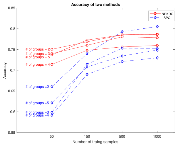
Figure 4: The accuracy rates of two methods.

4 Real Data Examples

4.1 Anuran Species Classification

Anuran calls data set was used in several classification tasks related to the challenge of anuran species recognition through their calls (see Dheeru and Karra Taniskidou, 2017), and was created by segmenting 60 audio records belonging to 4 different families, 8 genus, and 10 species, and each audio corresponds to one specimen. There are 7195 syllables identified from the 60 bioacoustics signals after segmenting, and each syllable is represented by a set of variables extracted by Mel-Frequency Spectral Coefficients (MFCCs), which performs a spectral analysis based on a triangular filter-bank logarithmically spaced in the frequency domain. Therefore, each sample in this data set is denoted by a variable set of MFCCS coefficients belonging to a special species. We focus on classification of the main 7 out of 10 species: Leptodactylus fuscus, Adenomera andreae, Adenomera hylaedactyla, Hyla minuta, Hypsiboas cinerascens, Hypsiboas cordobae, and Ameerega trivittata. In addition to the original dataset, we add 5 normally distributed noise attributes, with mean 0 and variance 1, as the irrelevant variables. In each run, we randomly select 100 and 50 examples from each species as the training and testing (evaluation) data, respectively, and report the results are based on 100 replications.

Figure 5 shows the box-plots of the mean predicted bandwidths with noise variables based on 100 trials, where the bandwidths of the last 5 added noise variables remain large, and the other bandwidths shrink as expected. This result indicates that the last 5 variables are irrelevant, which is consistent with our setup, and the proposed method successfully detects the relevant variables in this example. Table 9(b) summarizes the classification performance of the proposed NPKDC-vd method with both the original data and the data with 5 additional irrelevant variables. The results with the original data are used as our comparison baseline. Note that there are 3 popularly used performance indexes: accuracy, specificity, and precision, in this table. The results of NPKDC-vd show about $3\%$ drop in accuracy and precision when there are irrelevant variables in the data set, and specificity remains similar. The differences in results of NPKDC-vd between these two data sets are not statistically significant. Table 9(b) shows results of SVM and SVMfs under a similar setup. If we are only interested in classification accuracy, then SVMfs is the best choice in this example. However, SVMfs is built on multiple binary classifiers, and cannot have good interpretation ability. Thus, it provides less information about each class.

We summarize the means of Z-scores of the predicted bandwidths for all variables in Table 10. Most of the variables are identified. However, we found that besides the added irrelevant variables, some original variables such as Variable 1 and 2 in Hypsiboas Cordobae, and Ameerega Trivittata species are also regarded as irrelevant, which are new findings, and were not reported in the literature before.

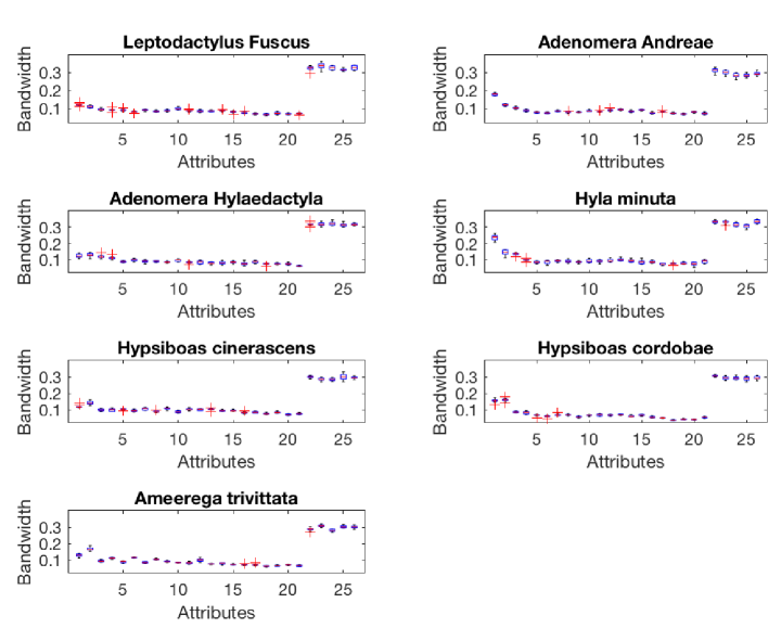
Figure 5: The box-plots of mean predicted bandwidths for anuran calls.

Table 9: Classification results of anuran species.

(a) Classification results of NPKDC-vd

	Original dataset			Extended dataset
	(without noise variables)			(with noise variables)
	Accuracy	Precision	Specificity	Accuracy	Precision	Specificity
mean	0.9155	0.9173	0.9859	0.8741	0.8807	0.9790
Std	0.0124	0.0019	0.0021	0.0142	0.0135	0.0024

(b) Classification results of SVM

	Original dataset			Extended dataset
	(without noise features)			(with noise features)
	Accuracy	Precision	Specificity	Accuracy	Precision	Specificity
mean	0.7606	0.9071	0.9734	0.7488	0.9081	0.9721
Std	0.0806	0.0118	0.0090	0.0895	0.0132	0.0099

Table 10: Anuran Calls: The means of Z-scores of the mean predicted bandwidths for all attributes, where the cells with gray background are relevant variables.

	1	2	3	4	5	6	7	8	9
Leptodactylus Fuscus	-0.14	-0.27	-0.38	-0.44	-0.37	-0.47	-0.43	-0.57	-0.44
Adenomera Andreae	0.53	-0.04	-0.33	-0.39	-0.59	-0.59	-0.45	-0.59	-0.55
Adenomera Hylaedactyla	-0.24	-0.27	-0.28	-0.29	-0.53	-0.24	-0.48	-0.46	-0.55
Hyla Minuta	0.80	-0.10	0.01	-0.43	-0.64	-0.58	-0.62	-0.51	-0.60
Hypsiboas Cinerascens	-0.11	0.06	-0.31	-0.40	-0.42	-0.55	-0.23	-0.57	-0.40
Hypsiboas Cordobae	0.29	0.53	-0.26	-0.35	-0.44	-0.57	-0.40	-0.56	-0.58
Ameerega Trivittata	0.08	0.20	-0.28	-0.40	-0.50	-0.22	-0.55	-0.37	-0.36
	10	11	12	13	14	15	16	17	18
Leptodactylus Fuscus	-0.30	-0.43	-0.41	-0.51	-0.45	-0.55	-0.62	-0.64	-0.62
Adenomera Andreae	-0.47	-0.50	-0.43	-0.46	-0.55	-0.47	-0.58	-0.59	-0.67
Adenomera Hylaedactyla	-0.41	-0.55	-0.45	-0.48	-0.49	-0.49	-0.58	-0.61	-0.64
Hyla minuta	-0.50	-0.47	-0.49	-0.45	-0.50	-0.54	-0.56	-0.62	-0.72
Hypsiboas Cinerascens	-0.59	-0.53	-0.46	-0.49	-0.50	-0.46	-0.73	-0.56	-0.65
Hypsiboas Cordobae	-0.55	-0.49	-0.47	-0.51	-0.48	-0.55	-0.68	-0.68	-0.71
Ameerega Trivittata	-0.49	-0.52	-0.39	-0.63	-0.48	-0.65	-0.65	-0.64	-0.71
	19	20	21	22	23	24	25	26
Leptodactylus Fuscus	-0.59	-0.65	-0.66	2.09	1.81	2.10	1.98	1.96
Adenomera Andreae	-0.72	-0.63	-0.65	2.03	1.92	1.93	1.99	1.85
Adenomera Hylaedactyla	-0.63	-0.60	-0.67	2.02	1.87	2.08	2.06	1.90
Hyla Minuta	-0.71	-0.69	-0.62	1.90	1.95	1.83	2.01	1.85
Hypsiboas Cinerascens	-0.60	-0.70	-0.61	1.90	2.15	1.92	1.84	2.04
Hypsiboas Cordobae	-0.73	-0.75	-0.65	1.96	2.06	1.78	1.92	1.89
Ameerega Trivittata	-0.69	-0.74	-0.79	1.95	1.97	2.06	1.93	1.84

Table 11: The probabilities of relevant variable identified by sequential variable selection, based on 1000 iterations, where the cells with gray background are variables with probability larger than 0.5

	1	2	3	4	5	6	7	8	9	10
1$\sim$10	0.1100	0.2000	0.2200	0.2900	0.3900	0.5000	0.4900	0.4100	0.4400	0.3400
	11	12	13	14	15	16	17	18	19	20
1$\sim$10	0.2700	0.1300	0.0900	0.0300	0.0100	0.0000	0.0000	0.0000	0.0000	0.0000
	21	22	23	24	25	26	27	28	29	30
1$\sim$10	0.0000	0.0000	0.0000	0.0000	0.0000	0.0000	0.0000	0.0000	0.0000	0.0000

4.2 Handwritten digit dataset

We use a subset from the MINST database of handwritten digits, where digits have been size-normalized and centered on a fixed-size image. We randomly select 100 gray images from this data set, for training, and another 100 images for testing from this database. (For the details about this database, please refer to LeCun et al. (2010).)

We resize each handwritten digit image to $64=8\times 8$ pixels, and treat each pixel as a variable. It becomes a 10-class classification problem through 64-dimensional density estimation when applying the proposed method. Table 12(b) shows the classification results of NPKDC-vd, where accuracy, precision, and specificity for all digits are greater than $95\%$, Table 12(b) shows the results of both SVM and SVMfs. From Table 12, we found that NPKDC-vd largely outperforms these two SVM-based methods in all three measurements, since the relations among classes in this example are rather complicated, and binary-classifier-based methods will suffer from complicated “voting-like” schemes.

Table 13 shows the means of Z-scores of the mean predicted bandwidths for all 64 attributes/pixels. The corresponding bandwidths of the relevant pixels could drop to a very small value. Moreover, because the background pixels of the image data have a density close to a point mass, instead of a uniform distribution, the variables with large interquartile ranges (IQR) are irrelevant. Figures of the box-plots for the mean of the selected bandwidths of the testing images based on 100 trials are in Supplementary, which provides similar information as in Table 13. The bandwidths of variables in this situation are the pixels on the edges of the image, such as 1, 8, 9, 16, 17, 24, 25, 32, 33, 40, 41, 48, 49, 56, 57, and 64, and their IQRs are usually large (see also Figures S.1 and S.2 in Supplementary). Table 14 shows the probabilities of relevant variable identification by SVM with sequential variable selection, based on 1000 iterations, for handwritten digits. We can see that the pixels/variables identified via the sequential variable selection of SVMfs scatter around all pixels, and cannot focus on some particular variables for each class (digit). Thus, in this case, SVMfs cannot provide neither stable information about each class, nor satisfactory classification performance.

Table 12: Classification results of handwritten digit dataset.

(a) Classification results of NPKDC-vd.

	Accuracy	Precision	Specificity
mean	0.9698	0.9966	0.9797
Std	0.0047	0.0005	0.0030

(b) Classification results of SVM and SVMfs

	SVM			SVMfs (with feature selection)
	Accuracy	Precision	Specificity	Accuracy	Precision	Specificity
mean	0.2739	0.8721	0.9193	0.7606	0.9071	0.9734
Std	0.0227	0.0303	0.0025	0.0806	0.0118	0.0090

Table 13: Handwritten Digits: The mean Z-scores of the mean predicted bandwidths for all attributes. The cells with gray background are irrelevant variables for its corresponding digit.

Digits	Attribute
	1	2	3	4	5	6	7	8	9	10	11	12	13
1	-0.80	-0.77	0.81	1.07	1.17	1.12	-0.40	-0.80	-0.80	-0.33	0.90	0.02	-0.38
2	-1.18	0.04	1.05	0.71	0.95	-0.82	-1.16	-1.18	-1.18	1.12	0.40	0.77	0.93
3	-1.27	-0.12	0.98	0.50	0.88	0.91	-0.98	-1.25	-1.27	1.02	0.70	0.93	0.81
4	-0.94	-0.93	-0.75	0.72	0.80	0.66	-0.78	-0.87	-0.94	-0.87	0.26	0.65	0.75
5	-1.22	-0.17	0.97	0.91	0.80	0.92	0.94	-1.17	-1.22	0.75	0.18	0.82	0.69
6	-1.15	-1.15	0.32	1.02	1.11	-0.34	-1.15	-1.15	-1.15	-1.06	1.14	0.47	0.95
7	-1.11	-0.91	1.07	0.87	0.46	0.78	1.13	-0.36	-1.11	-0.47	1.19	1.09	1.03
8	-1.28	-1.04	0.80	0.61	0.69	0.89	-0.70	-1.28	-1.27	0.73	0.50	0.85	0.85
9	-1.26	-0.86	0.86	0.81	0.85	0.69	-0.73	-1.21	-1.26	0.64	0.35	0.86	0.78
10	-1.27	-1.26	0.91	0.74	1.11	0.39	-1.25	-1.27	-1.27	0.13	0.87	1.02	0.99
Digits	Attribute
	14	15	16	17	18	19	20	21	22	23	24	25	26
1	1.20	-0.22	-0.80	-0.79	-0.22	1.23	-0.23	-0.65	1.15	-0.43	-0.80	-0.78	0.01
2	0.27	-1.13	-1.18	-1.18	1.03	1.17	0.96	0.90	0.49	-1.09	-1.18	-1.18	0.05
3	0.99	-0.51	-1.26	-1.27	0.49	0.85	0.78	0.92	1.05	-0.71	-1.27	-1.27	-0.98
4	0.05	0.01	-0.64	-0.94	-0.56	0.73	0.76	0.57	0.69	0.90	-0.59	-0.94	0.42
5	0.90	0.62	-1.19	-1.20	0.89	0.33	0.84	0.53	-0.31	-1.14	-1.22	-1.22	0.88
6	-0.49	-1.15	-1.15	-1.15	-0.14	0.90	1.06	-0.81	-1.14	-1.15	-1.15	-1.15	0.70
7	0.66	0.96	-0.55	-1.11	-0.86	-0.21	-0.56	0.90	0.80	0.86	-0.96	-1.11	-0.67
8	0.73	0.60	-1.28	-1.27	0.88	0.70	0.76	0.88	0.71	0.54	-1.28	-1.28	0.33
9	0.97	0.13	-1.13	-1.26	0.90	0.73	0.82	0.89	0.70	0.51	-1.14	-1.26	0.59
10	1.06	-0.81	-1.27	-1.27	1.03	0.38	0.94	0.52	0.78	0.73	-1.27	-1.27	0.86
Digits	Attribute
	27	28	29	30	31	32	33	34	35	36	37	38	39
1	1.23	-0.43	-0.61	1.13	-0.48	-0.80	-0.80	0.02	1.26	-0.32	-0.25	1.26	-0.65
2	0.49	0.76	0.94	0.50	-1.17	-1.18	-1.18	-1.09	-0.62	0.99	0.86	-0.01	-1.17
3	0.44	1.02	-0.01	0.98	-1.00	-1.27	-1.27	-1.17	0.17	1.02	0.86	0.68	0.73
4	0.27	0.93	0.49	0.70	0.83	-0.83	-0.93	0.80	-0.32	0.90	0.83	-0.37	0.92
5	-0.16	0.53	0.58	0.54	-0.58	-1.22	-1.22	0.39	0.99	0.69	0.83	0.87	0.20
6	0.55	1.17	0.31	-0.21	-1.12	-1.15	-1.15	0.91	0.30	0.92	0.93	1.05	0.34
7	0.86	1.17	0.81	0.65	1.02	-1.08	-1.11	0.06	1.13	0.37	-0.29	0.82	1.15
8	0.76	0.43	0.30	0.81	-0.40	-1.28	-1.28	-0.75	0.85	0.15	0.60	0.39	-0.57
9	0.77	0.83	0.84	0.08	0.94	-1.26	-1.26	-1.13	0.36	0.77	0.90	0.70	0.82
10	0.98	0.02	-1.14	1.09	0.49	-1.27	-1.27	0.88	1.06	-0.72	-1.14	1.10	0.43
Digits	Attribute
	40	41	42	43	44	45	46	47	48	49	50	51	52
1	-0.80	-0.80	-0.30	1.05	-0.20	-0.28	1.17	-0.64	-0.80	-0.80	-0.64	0.89	-0.32
2	-1.18	-1.18	-1.01	0.52	0.87	1.02	-0.22	-0.74	-1.18	-1.16	0.11	0.95	-0.31
3	-1.27	-1.27	-1.25	-0.39	-0.76	0.22	0.95	0.84	-1.26	-1.27	0.26	1.00	1.00
4	-0.94	-0.46	0.72	0.44	0.72	-0.23	0.55	0.42	-0.94	-0.74	-0.10	0.19	0.80
5	-1.22	-1.22	-1.14	-0.87	-0.74	0.48	0.79	0.36	-1.21	-1.22	0.02	1.01	0.94
6	-1.15	-1.15	0.79	0.05	1.08	1.02	1.04	1.12	-0.92	-1.15	-0.55	1.05	0.97
7	-1.11	-1.11	-0.42	0.62	0.86	0.93	0.72	-0.41	-1.11	-1.11	-1.07	0.79	0.53
8	-1.28	-1.28	-0.12	0.83	0.89	0.77	0.81	-0.13	-1.28	-1.28	-0.25	0.77	0.88
9	-1.26	-1.26	-1.16	-0.92	-0.97	-0.15	0.96	0.70	-1.25	-1.26	-0.47	0.66	0.94
10	-1.27	-1.27	0.75	0.74	-0.00	-0.26	1.00	0.96	-1.27	-1.27	-0.24	0.79	1.12
Digits	Attribute
	53	54	55	56	57	58	59	60	61	62	63	64
1	-0.30	1.18	0.03	-0.79	-0.80	-0.78	0.83	0.94	1.18	1.13	0.59	-0.79
2	1.02	1.12	1.11	-0.35	-1.17	0.05	1.06	0.82	0.95	1.01	1.10	0.21
3	1.05	0.53	1.03	-1.22	-1.27	-0.22	1.03	0.70	0.77	1.04	0.15	-1.27
4	0.26	0.93	-0.78	-0.94	-0.94	-0.90	-0.76	0.95	0.68	0.49	-0.94	-0.94
5	0.75	0.79	0.17	-1.21	-1.22	-0.19	0.99	0.31	0.80	0.68	-1.01	-1.21
6	1.14	1.09	1.06	-0.43	-1.15	-1.15	0.51	1.02	0.52	1.00	1.11	-0.86
7	0.94	-0.99	-1.11	-1.11	-1.11	-0.94	1.08	0.92	0.06	-1.08	-1.11	-1.11
8	0.82	0.77	0.25	-1.28	-1.28	-1.20	0.82	0.60	0.71	0.86	-0.53	-1.27
9	0.86	0.67	0.55	-1.23	-1.26	-0.98	0.72	0.58	0.76	0.77	-0.09	-1.26
10	1.12	0.63	0.46	-1.27	-1.27	-1.27	0.82	0.80	0.76	1.00	-1.04	-1.27

Table 14: The probabilities of relevant variable identification of SVM with sequential variable selection for handwritten digits based on 1000 runs.

Attribute	1	2	3	4	5	6	7	8	9	10	11	12	13
Prob.	0	0.16	0.19	0.19	0.18	0.34	0.19	0.18	0.11	0.10	0.74	0.21	0.18
Attribute	14	15	16	17	18	19	20	21	22	23	24	25	26
Prob.	0.42	0.09	0.16	0.04	0.09	0.72	0.66	0.76	0.96	0.16	0.11	0	0.18
Attribute	27	28	29	30	31	32	33	34	35	36	37	38	39
Prob.	0.65	0.63	0.37	0.49	0.52	0	0	0.1	0.17	0.24	0.56	0.39	0.39
Attribute	40	41	42	43	44	45	46	47	48	49	50	51	52
Prob.	0	0.01	0.19	1	0.73	0.43	0.32	0.21	0.03	0.03	0.14	0.09	0.33
Attribute	53	54	55	56	57	58	59	60	61	62	63	64
Prob.	0.41	0.48	0.13	0.07	0	0.12	0.16	0.22	0.27	0.63	0.40	0.15

5 Summary

The relative position of classes in the variable-space of a multiple-class classification problem is usually complicated. Hence, some complicated modeling procedures are preferred for their classification performance. Using a voting scheme via building many binary classifiers is another choice. However, this kind of approach usually aims at high prediction power, and sacrifices the “model interpretation” ability, which is important from many classification application perspectives. If we only aim our classification goal at classification performance, such as accuracy, specificity, sensitivity/precision, then finding only a set of variables for all classes, via using a complicated model, could be an easy way out. Nevertheless, we will have less power about model interpretation when the relations among classes are complicated, and this goal is even more difficult to be achieved when data sets have lengthy variables. Thus, when the model-interpretation ability is indispensable to an application, deciding class-specific variable sets to clarify the classification rules of models is important in addition to the conventional classification performance measures. In this study, we adopt NPKDC-vd for multiple-class classification, and shows that the error rate of this method approaches to that of the Bayes rule, asymptotically. Moreover, through local bandwidths of density estimation, we integrate such a posterior density estimation procedure with a variable selection scheme such that we are able to identify the individual high impact variable set for each class, such that the proposed classification rule are easier to be understood, and we can have a better description of the character of each class. In the numerical examples, we see that the proposed method has a satisfactory classification performance with only a limited increase of computational burden, and the “interpretation” of each class is largely improved, especially for the examples with complicated relative positions among classes. Because we can separately calculate the local bandwidths within each class, the computational efficiency can be further improved via parallel computing methods, and can be easily implemented via machines with a multi-core CPU. Moreover, because using the bandwidth to select the relevant variables is a promising approach, we suggest a two-step approach such that we can first filter out the irrelevant variables to reduce variable size in advance, then apply the proposed algorithm with the rest variables. This approach can be useful for problems with a small sample size but a large number of variables. Since there will need different considerations for filtering out variables in the first stage, and will go beyond the scope of the current project. Thus, we will study this problem in our future studies, and will report its results elsewhere.

References

- Ancukiewicz (1998) Ancukiewicz M (1998) An unsupervised and nonparametric classification procedure based on mixtures with known weights. Journal of Classification 15(1):129–141
- Bagheri, Montazer, and Escalera (2012) Bagheri MA, Montazer and S. Escalera (2012) Error correcting output codes for multiclass classification: Application to two image vision problems, The 16th CSI International Symposium on Artificial Intelligence and Signal Processing (AISP 2012), 2012, 508-513.
- Berger (1999) Berger A (1999) Error-correcting output coding for text classification. In IJCAI-99: Workshop on machine learning for information filtering.
- Devroye and Gyorfi (1985) Devroye L, Gyorfi L (1985) Nonparametric Density Estimation: The L1 View. Wiley Interscience Series in Discrete Mathematics, Wiley
- Devroye and Wagner (1976) Devroye L, Wagner TJ (1976) A distribution-free performance bound in error estimation (corresp.). IEEE Trans Information Theory 22(5):586–587
- Dheeru and Karra Taniskidou (2017) Dheeru D, Karra Taniskidou E (2017) UCI machine learning repository
- Fan and Fan (2008) Fan J, Fan Y (2008) High-dimensional classification using features annealed independence rules. Ann Statist 36(6):2605–2637
- George and Langley (1995) George J, Langley P (1995) Estimating continuous distributions in bayesian classifiers. In: Proceedings of the Eleventh Conference on Uncertainty in Artificial Intelligence, Morgan Kaufmann, pp 338–345
- Greblicki and Pawlak (1983) Greblicki W, Pawlak M (1983) Almost sure convergence of classification procedures using hermite series density estimates. Pattern Recognition Letters 2(1):13–17
- Gu et al. (2013) Gu C, Jeon Y, Lin Y (2013) Nonparametric density estimation in high-dimensions. Statistica Sinica 23(3):1131–1153
- Hall and Kang (2005) Hall P, Kang KH (2005) Bandwidth choice for nonparametric classification. Ann Statist 33(1):284–306
- Hall and Wand (1988) Hall P, Wand MP (1988) Minimizing l1 distance in nonparametric density estimation. Journal of Multivariate Analysis 26(1):59 – 88
- Har-Peled et al. (2002) Har-Peled S, Roth D, Zimak D (2002) Constraint classification for multiclass classification and ranking. In: Advances in Neural Information Processing Systems 15, pp 785–792
- Hochberg and Tamhane (1987) Hochberg Y, Tamhane AC (1987) Multiple Comparison Procedures. John Wiley & Sons, Inc., New York, NY, USA
- James and Hastie (1998) James G, Hastie T (1998) The Error Coding Method and PICTs, Journal of Computational and Graphical Statistics, 7(3), 377–387.
- Kobos and Mandziuk (2011) Kobos M, Mandziuk J (2011) Multiple-resolution classification with combination of density estimators. Connect Sci 23(4):219–237
- Kundu and Martinsek (1997) Kundu S, Martinsek AT (1997) Bounding the l1 distance in nonparametric density estimation. Annals of the Institute of Statistical Mathematics 49(1):57–78
- LeCun et al. (2010) LeCun Y, Cortes C, Burges C (2010) Mnist handwritten digit database. ATT Labs [Online] Available: http://yannlecuncom/exdb/mnist 2
- Leiva-Murillo and Artés-Rodríguez (2012) Leiva-Murillo JM, Artés-Rodríguez A (2012) Algorithms for maximum-likelihood bandwidth selection in kernel density estimators. Pattern Recognition Letters 33(13):1717–1724
- Liu et al. (2007) Liu H, Lafferty J, Wasserman L (2007) Sparse nonparametric density estimation in high dimensions using the rodeo. In: Meila M, Shen X (eds) Proceedings of the Eleventh International Conference on Artificial Intelligence and Statistics, PMLR, San Juan, Puerto Rico, vol 2, pp 283–290
- Liu et al. (2008) Liu J, Ranka S, Kahveci T (2008) Classification and feature selection algorithms for multi-class cgh data. Bioinformatics 24(13):86–95
- Lugosi and Nobel (1996) Lugosi G, Nobel A (1996) Consistency of data-driven histogram methods for density estimation and classification. Ann Statist 24(2):687–706
- Mechbal et al. (2015) Mechbal N, Uribe JS, Rebillat M (2015) A probabilistic multi-class classifier for struc- tural health monitoring. Mechanical Systems and Signal Processing pp 106 – 123
- Scott and Sain (2005) Scott D, Sain S (2005) Multidimensional density estimation. In: Rao C, Wegman E, Solka J (eds) Handbook of Statistics, vol 24, Elservier, Amsterdam, pp 229 – 261
- Shao et al. (2011) Shao J, Wang Y, Deng X, Wang S (2011) Sparse linear discriminant analysis by thresholding for high dimensional data. Ann Statist 39(2):1241–1265
- Sugiyama (2010) Sugiyama M (2010) Superfast-trainable multi-class probabilistic classifier by least-squares posterior fitting. IEICE Transactions 93-D(10):2690–2701
- Sugiyama et al. (2012) Sugiyama, M, Suzuki, T, Kanamori, T (2012) Density Ratio Estimation in Machine Learning. Cambridge: Cambridge University Press.
- Tomczak and Zieba (2015) Tomczak JM, Zieba M (2015) Probabilistic combination of classification rules and its application to medical diagnosis. Machine Learning 101:105 – 135
- Tukey (1949) Tukey JW (1949) Comparing individual means in the analysis of variance. Biometrics 5(2):99–114
- Van Ryzin (1966) Van Ryzin JR (1966) The compound decision problem with finite loss matrix. Ann Math Statist 37(2):412–424
- Yang et al. (2010) Yang J, Yu P, Kuo B (2010) A nonparametric feature extraction and its application to nearest neighbor classification for hyperspectral image data. IEEE Transactions on Geoscience and Remote Sensing 48(3):1279–1293
- Yang (1999) Yang Y (1999) Minimax nonparametric classification. ii. model selection for adaptation. IEEE Transactions on Information Theory 45(7):2285–2292
- Zhang (2017) Zhang Z (2017) Approaches to feature identification and feature selection for binary and multi-class classification. PhD thesis, University of Minnesota