Density functional theory plus dynamical mean field theory within the framework of linear combination of numerical atomic orbitals: Formulation and benchmarks

Abstract

The combination of density functional theory with dynamical mean-field theory (DFT+DMFT) has become a powerful first-principles approach to tackle strongly correlated materials in condensed matter physics. The wide use of this approach relies on robust and easy-to-use implementations, and its implementation in various numerical frameworks will increase its applicability on the one hand and help crosscheck the validity of the obtained results on the other. In the work, we develop a formalism within the linear combination of numerical atomic orbital (NAO) basis set framework, which allows for merging NAO-based DFT codes with DMFT quantum impurity solvers. The formalism is implemented by interfacing two NAO-based DFT codes with three DMFT impurity solvers, and its validity is testified by benchmark calculations for a wide range of strongly correlated materials, including 3d transition metal compounds, lanthanides, and actinides. Our work not only enables DFT+DMFT calculations using popular and rapidly developing NAO-based DFT code packages, but also facilitates the combination of more advanced beyond-DFT methodologies available in this codes with the DMFT machinery.

I INTRODUCTION

The understanding of strong correlations among electrons in realistic materials is of great importance for both fundamental science and technological applications. The strong electron correlations trigger a variety of exotic phenomena, which provide a fruitful avenue for designing novel materials [1, 2, 3]. Kohn-Sham (KS) density functional theory (DFT) [4, 5] under local-density approximation (LDA) and generalized gradient approximation (GGA) has achieved remarkable success in describing a very wide range of materials. However, these approximations are found to be inadequate for correctly describing strongly correlated materials, e.g., 3d transitional metal compounds, lanthanides, actinides, quantitatively or even qualitatively [6, 7, 8, 9]. To overcome this limitation, the so-called DFT+DMFT method that merges DFT and many-body technique based dynamical mean-field theory (DMFT) has been developed [10, 11, 12, 13, 7, 14, 15, 8, 9]. Various studies have shown the prominent strength of DFT+DMFT in describing electronic structures of strongly correlated materials. DFT+DMFT has thus becoming a promising method of choice in studying realistic strongly correlated materials with certain predictive power. [16, 17, 18, 19, 8, 9]

Comparing to DFT+U [6, 20, 21], a method that shares similar spirit as DFT+DMFT and is available in nearly all popular DFT code packages, DFT+DMFT is not only computationally more expensive, but also relatively more difficult to access for normal users. Implementing DFT+DMFT with well-defined local orbital basis and in a way that doesn’t requires much expertise from users is, thus, of practical importance for promoting the methodology in studying realistic correlated materials. One of the key issues in the implementation of DFT+DMFT scheme is the definition of local correlated orbitals, in terms of which the DMFT impurity problem is defined and solved. Many-body corrections to the KS Hamiltonian exist only in this subspace. As a result, the choice of local correlated orbitals has a noticeable influence on the obtained DFT+DMFT results at the quantitative level.

In early days, DFT+DMFT was implemented within the linear muffin-tin orbital (LMTO) basis set framework [14, 15, 16, 22, 23], where the local LMTOs were chosen as the basis orbitals hosting strongly correlated d or f electrons. Later, different Wannier-type orbitals, such as projective Wannier functions [24] and maximally localized Wannier functions, were used to define the local orbitals [25, 26]. As for plane-wave based DFT, Amadon et al. [27, 28] used the all-electron atomic partial waves within the projector augmented wave (PAW) framework or pseudoatomic wave functions as the local correlated orbitals. Within the linearized augmented plane-wave (LAPW) method, Aichhorn et al. [29], and Haule et al. and Kim [30] independently developed projector schemes that convert the KS orbital space to local correlated subspace. We note that, in recent years, the underlying embedding idea of DMFT has been used in broader sense whereby the embedded cluster is solved in a ab initio way using beyond-DFT approaches such as $GW$ or coupled-cluster method, whereas the environment is treated using less advanced approaches [31, 32, 33].

In recent years, numerical atomic orbitals (NAOs) have been employed as the basis set choice in several first-principles software packages [34, 35, 36, 37, 38]. Unlike most other basis sets, the linear combination of NAOs represents a versatile framework that can be used in both all-electron and pseudopotential-based DFT calculations. Past experience indicates that NAOs are an efficient basis set choice not only for conventional ground-state calculations, but also for functionalities that go beyond conventional DFT calculations whereby explicit two-electron Coulomb integrals and/or unoccupied KS states are needed [39, 40, 41, 42]. In this regard, it is highly desirable to develop computational schemes within the NAO basis set framework that enables a convenient merging of first-principles and model-Hamiltonian based approaches. In case of DFT+$U$, several NAO-based implementations have been reported previously [43, 44, 45]. However, in case of DFT+DMFT, only one recent work within the pseudoatomic orbital basis sets (i.e., NAOs tailored for pseudopotential-based calculations) was reported by Sim and Han [46]. In their work, these authors proposed to use the so-called natural atomic orbitals – the eigen-orbitals for the local density matrix – to define the local correlated orbitals. In the present work, we develop a projection scheme that allows to conveniently interface the NAO-based DFT codes and the DMFT impurity solvers and thus enables NAO-based DFT+DMFT calculations. We test the efficacy of such a scheme for the all-electron FHI-aims code [37] and the norm-conserving pseudopotential based ABACUS code [38], interfaced with three different DMFT impurity solver packages. Consistent results are obtained for transition metal compounds, including both correlated metals (SrVO₃) and Mott insulators (NiO and MnO), rare-earth systems (Ce metal and Ce₂O₃), and actinides (Pu₂O₃ and PuO₂). Our work thus extends the reach of the NAO-based numerical framework to treat strongly correlated materials.

This paper is organized as follows. Sec. II focuses on the DFT+DMFT formalism. After introducing the general DFT+DMFT formulation, we present our definition of local correlated orbitals within the NAO framework. This is followed by a discussion of the self-consistency scheme of our DFT+DMFT implementation. In Sec. III, we benchmark the validity of our DFT+DMFT formalism and implementation over a wide range of strongly correlated materials, i.e., 3d-systems SrVO₃, MnO and NiO, 4f-systems Ce metal and Ce₂O₃, and 5f-systems Pu₂O₃ and PuO₂. Sec. IV concludes this paper.

II THEORETICAL FORMULATION

II.1 General DFT+DMFT formalism

Combining DFT with DMFT is not straightforward conceptually as the two theories are formulated in different forms and in different Hilbert spaces. In KS-DFT, one needs to self-consistently solve an effective single-particle problem, whereby (for periodic systems) a KS Hamiltonian is constructed and solved separately at each individual ${\bf k}$ point in the Brillouin zone (BZ). On the other hand, DMFT is a real-space approach developed to solve the lattice Hamiltonian models in which the on-site two-electron interactions are explicitly included. Furthermore, as a first-principles approach, DFT accounts for all the chemical details in the systems and include all (at least valence) electrons in the calculations. In contrast, only the strongly correlated electrons sitting energetically in the vicinity of the Fermi level, relevant for the low-energy physics, are included in the model Hamiltonian and treated explicitly in DMFT. As such, key quantities like charge density, density matrix, and Green functions all have different representations in DFT and DMFT, impeding a straightforward combination of the two approaches. One solution to address this challenge, as detailed below, is to define a suitable projector to convert the key quantities back and forth between the two representations. As a side note, in the following we only focus on the general formalism of DFT+DMFT, without going into a detailed account of DMFT itself in this paper. Interested readers are referred to Refs. [10, 12, 7, 8, 9, 47] for a detailed discussion of this theory.

Briefly, in the DFT+DMFT formalism, the Green functions defined in the correlated subspace are the central objects gluing the two theories. There are two kinds of interacting Green functions defined in the corrected subspace: One is the impurity Green function $G^{imp}$ determined by solving the impurity problem in Anderson impurity model, describing a single site with on-site Coulomb interactions and coupled to a mean-field electron bath. The another one, denoted as $G^{loc}$, is the on-site term of the lattice Green function, which is essentially the the Green function of the correlated site described by the Hubbard model and is obtained by projecting the Green function in the full Hilbert space into the correlated subspace. The fundamental requirement in DMFT is that the “on-site” Green function of the lattice problem and that of the Anderson impurity model are equal,

$$G^{loc}=G^{imp}\,,$$ (1)

which is achieved via the DMFT self-consistency cycle.

In the DFT+DMFT scheme, the single-particle effective Hamiltonian in the full Hilbert space can be expressed as

$$\hat{H}=\hat{H}_{\mathrm{KS}}+\hat{\Sigma}-\hat{H}_{\mathrm{dc}}\,,$$ (2)

where $\hat{H}_{\mathrm{KS}}$ is the non-interacting KS Hamiltonian, $\hat{\Sigma}$ the self-energy which encodes all the many-body complexities arising from strong electron correlations and are nonzero only for correlated orbitals. Finally, $\hat{H}_{\mathrm{dc}}$ is the double-counting term, which is introduced to discount the interactions among correlated electrons that have been included in a static mean-field level in $\hat{H}_{\mathrm{KS}}$.

Starting from the Hamiltonian Eq. (2), the key issue in the combination of DFT and DMFT is the downfolding (projecting) of the physical quantities from the full KS space to the local correlated space, and the upfolding (embedding) of these quantities from the local space to the full space. Mathematically, the local interacting Green function $G^{loc}$ can be obtained through a projection procedure. In the literature, two different projection procedures have been used. The first one can be seen as a “Hamiltonian projection”, whereby a tight-binding Hamiltonian is first obtained from the KS Hamiltonian by projecting the latter into the correlated subspace,

$$H_{mm^{\prime}}^{TB}({\bf k})=\langle\phi_{m{\bf k}}|\hat{H}_{\mathrm{KS}}|\phi_{m^{\prime}{\bf k}}\rangle\,.$$ (3)

Here $\phi_{m{\bf k}}$ is the Bloch-summed local orbitals with $m$ denoting an orbital index in the correlated subspace. In the second step, the local interacting Green function can be directly calculated from this tight-binding Hamiltonian as

$$G_{mm^{\prime}}^{loc}(i\omega_{n})= \sum_{{\bf k}}\frac{1}{N_{\bf k}}\left[(i\omega_{n}+\mu)I-H^{TB}({\bf k})\right.$$ (4)

$$\left.-\Sigma(i\omega_{n})+H_{\mathrm{dc}}\right]_{mm^{\prime}}^{-1}\,,$$

where $N_{\bf k}$ is the is the number of ${\bf k}$ points in the first Brillouin zone, equivalent to the number of unit cells in the Born-von Kármán supercell. In Eq. (4), $\mu$ is the chemical potential, $I$ an identity matrix, and $[\cdots]^{-1}$ denotes the matrix inversion which is taken within the correlated subspace. Here and below, we employ the Matsubara Green function formalism where $\omega_{n}=(2n+1)\pi/\beta$ are the discrete frequency points along the imaginary frequency axis, with $\beta=1/k_{B}T$ being the inverse temperature. The spectroscopy results on the real frequency axis are obtained via analytical continuations. The above procedure to compute the local interacting Green function is the so-called tight-binding Hamiltonian method.

In the second scheme, one first constructs the interacting Green function in the full Hilbert space as

$$G_{ij}({\bf k},i\omega_{n})=\left[(i\omega_{n}+\mu)I-H({\bf k})\right]_{ij}^{-1}\,,$$ (5)

where the Hamiltonian matrix $H_{ij}({\bf k})=\langle\chi_{i,{\bf k}}\mid\hat{H}\mid\chi_{j,{\bf k}}\rangle$ is the representation of the interacting Hamiltonian operator introduced in Eq. (2) within an arbitrary orthonormal basis set $\mid\chi_{j,{\bf k}}\rangle$ expanding the full Hilbert space. While the matrix elements of the KS Hamiltonian $\hat{H}_{\mathrm{KS}}$ within such a basis set are given straightforwardly, those of $\hat{\Sigma}$ and $\hat{H}_{\mathrm{dc}}$ will be discussed later in Sec. II.3. Once the full-space lattice Green function is obtained, the local interacting Green function can be obtained through a projection procedure

$$G_{mm^{\prime}}^{loc}(i\omega_{n})=\sum_{{\bf k}}\frac{1}{N_{\bf k}}\sum_{ij}P_{ij}({\bf k},mm^{\prime})G_{ji}({\bf k},i\omega_{n})~{},$$ (6)

where the projector above is given by

$$P_{ij}({\bf k},mm^{\prime})=\langle\phi_{m}|\chi_{i{\bf k}}\rangle\langle\chi_{j{\bf k}}|\phi_{m^{\prime}}\rangle\,.$$ (7)

The construction of the local Green function via Eqs. (5)-(7) is known as the projector method.

The two methods discussed above to construct the local Green function differ in that the tight-binding Hamiltonian method projects the Hamiltonian matrix while the projector method projects the Green function. In the projector method, the matrix inversion is carried out in the full Hilbert space, as indicated in Eq. (5), and thus the interactions between the correlated electrons and the rest electrons are retained to some extent. On the other hand, within the tight-binding method, if one wants to describe the interaction between correlated electrons and the rest ones, e.g., studying the charge transfer process between the correlated orbitals and the bath, one has to enlarge the Hilbert space of the tight-binding Hamiltonian to encompass the extra itinerant electrons, and it will inevitably increases the computational complexity. In this work, we choose the projector method in our DFT+DMFT implementation.

The other key quantity in DFT+DMFT calculations is the interacting impurity Green function $G^{imp}$ in Eq. (1), corresponding to the local propagator of the effective single-impurity Anderson model, which describes a single site coupled to a bath that mimics the lattice environment at a mean-field level. Formally $G^{imp}$ satisfies the following relationship

$$G^{imp}_{mm^{\prime}}\left(i\omega_{n}\right)= [(i\omega_{n}+\mu)I-{\cal E}^{imp}-\Delta\left(i\omega_{n}\right)$$ (8)

$$-\Sigma^{imp}\left(i\omega_{n}\right)]_{mm^{\prime}}^{-1}\,,$$

where ${\cal E}^{imp}$ is the impurity energy level, $\Delta\left(i\omega_{n}\right)$ the so-called hybridization function characterizing the influence of the environment on the embedded impurity, and $\Sigma^{imp}\left(i\omega_{n}\right)$ the impurity self-energy. It should be noted that ${\cal E}^{imp}$ and $\Delta\left(i\omega_{n}\right)$ are matrices when there are multiple orbitals in the correlated subspace, which is typical in DFT+DMFT calculations. In this context, it is also customary to define a so-called Weiss Green function

$$\mathcal{G}_{mm^{\prime}}^{-1}(i\omega_{n})= G_{mm^{\prime}}^{-1}(i\omega_{n})+\Sigma_{mm^{\prime}}$$ (9)

$$= [(i\omega_{n}+\mu)I-{\cal E}^{imp}-\Delta\left(i\omega_{n}\right)]_{mm^{\prime}}~{},$$

which acts as the dynamical (energy-dependent) mean field that the impurity electrons experience, and encodes essentially the same information as the hybridization function $\Delta\left(i\omega_{n}\right)$. When the self-consistency in the DMFT loop is reached, the local Green function $G_{mm^{\prime}}^{loc}(i\omega_{n})$ and the local self-energy $\Sigma_{mm^{\prime}}(i\omega_{n})$ in Eq. (4) and (6) are equal to the impurity Green function $G^{imp}_{mm^{\prime}}(i\omega_{n})$ and the impurity self-energy $\Sigma^{imp}_{mm^{\prime}}(i\omega_{n})$, respectively.

The Weiss Green function together with the local Coulomb interactions defines the Anderson impurity model, which can be expressed in terms of an action [7]

$$S= \int_{0}^{\beta}d\tau\sum_{mm^{\prime}}c_{m}^{\dagger}(\tau)\mathcal{G}_{mm^{\prime}}^{-1}\left(\tau\right)c_{m^{\prime}}\left(\tau\right)$$ (10)

$$-\sum_{lmno}U_{lmno}\int_{0}^{\beta}d\tau c_{l}^{\dagger}(\tau)c_{n}(\tau)c_{m}^{\dagger}(\tau)c_{o}(\tau)~{},$$

where $c_{l}^{\dagger}(\tau)$, $c_{n}(\tau)$, etc., should be understood as the Grassmann variables, and $U_{lmno}$ is the on-site Coulomb interaction expressed within a set of local orbitals (labelled by $l,m,n,o$) spanning the correlated subspace. The action $S$ is essentially the integration of the Lagrangian over the imaginary time. For given $S$, the impurity Green function can be calculated as

$$G^{imp}_{mm^{\prime}}=-\frac{1}{\mathcal{Z}}\int\mathcal{D}\prod_{i}\left[c^{\dagger},c\right]c_{m}c_{m^{\prime}}^{\dagger}e^{-S}~{},$$ (11)

where $i$ runs over all $m$ indices, and $\mathcal{Z}$ is the partition function

$$\mathcal{Z}=\int\mathcal{D}\prod_{i}\left[c^{\dagger},c\right]e^{-S}\,.$$ (12)

The interacting impurity Green’s function defined via Eqs. (10-12) can then be obtained through a variety of numerical approaches – usually termed as impurity solvers. Up to date, several types of impurity solvers have been developed, including the quantum Monte Carlo (QMC) [13, 48, 49, 50], non-crossing approximation (NCA) [51, 52, 53], one-crossing approximation (OCA) [54, 55], exact diagonalization (ED) [56, 57], numerical renormalization group (NRG) [58, 59], etc. Among all these impurity solvers, continuous-time quantum Monte Carlo (CTQMC) [60, 61, 62, 63] provides access to both high and low energy scales and is effective for a wide class of realistic material calculations. Nowadays, the CTQMC, especially the hybridization expansion based CTQMC (CT-HYB), is the most popular impurity solver employed in DFT+DMFT calculations.

Once the interacting impurity Green function is determined, the impurity self-energy $\Sigma^{imp}(i\omega_{n})$ can be obtained via the Dyson equation $\Sigma^{imp}(i\omega_{n})=\left[\mathcal{G}(i\omega_{n})\right]^{-1}-\left[G^{imp}(i\omega_{n})\right]^{-1}$, which is usually done within the impurity solvers. This impurity self-energy will be taken as the updated local self-energy and fed into Eq. (3) and (4) or (2) and (5), from which a new local Green function and consequently a new Weiss Green’s function can be obtained. This is where a new iteration starts. This self-consistency loop keeps going until the self-energy reaches convergence or the local and impurity interacting Green function satisfies the self-consistency condition, i.e., Eq. (1).

II.2 Construction of the projector

Within the NAO basis set framework, it’s natural to take the $d$ or $f$-type NAOs that contribute most to the electronic states around the Fermi level as the the local correlated orbitals. These NAOs by construction are localized and atom-centered, and thus satisfy the usual requirement of correlated orbitals. In early DFT+DMFT implementations, analogous atomic-like orbitals like LMTOs were used. LMTOs are minimal basis sets in the sense that for each angular momentum channel there is only one radial basis function. In contrast with LMTOs, the NAO basis sets are of multi-$\zeta$ character meaning that there are more than one radial functions per angular momentum, thus offering a more accurate description of the electronic structure. In the past, the DFT+U method has been successfully implemented within NAO-based DFT codes [43, 44, 45], whereby it turns out to be a good practice to choose the most localized $d$ or $f$ basis functions as the correlated orbitals to apply the Hubbard $U$ correction. Thus the most localized $d$ or $f$ orbitals seems to span the correlated subspace rather well. In practice, since NAOs centering on neighboring atoms are non-orthogonal to each other, certain orthorgonalization procedure is needed to generate an orthonormal local basis set, which is convenient for DMFT calculations.

Below we shall discuss our procedure to construct the projector and local correlated orbitals to facilitate DFT+DMFT calculations within the NAO basis set framework. In analogy to the transformation between Bloch orbitals and Wannier orbitals, we define the following Bloch-summed atomic orbitals as

$$\Phi_{I,m}^{\bf{k}}({\bf r})=\frac{1}{\sqrt{N_{\bf k}}}\sum_{\mathbf{R}}e^{i\mathbf{k}\cdot\mathbf{R}}\phi_{I,m}\left({\bf r}-{\bm{\tau}}_{I}-\bf{R}\right)\,,$$ (13)

where $\phi_{I,m}\left({\bf r}-{\bm{\tau}}_{I}-\bf{R}\right)$ is a NAO located at atomic site $I$ in cell ${\bf R}$. Here the magnetic quantum number $m$ labels the different orbitals in the correlated angular moment channel, such as the five $d$ orbitals or seven $f$ orbitals.

Since NAOs on neighboring atomic sites are non-orthogonal to each other, it is obvious that the $\Phi_{I,m}^{{\bf k}}({\bf r})$’s defined in Eq. (13) with different $m$ are also non-orthogonal. The key next step is to employ the L$\ddot{\text{o}}$wdin orthonormalization procedure to $\Phi_{I,m}^{\mathbf{k}}$, i.e.,

$$\mid\tilde{\Phi}_{I,m}^{\mathbf{k}}\rangle=\sum_{I^{\prime}m^{\prime}}O^{-\frac{1}{2}}_{Im,I^{\prime}m^{\prime}}\left(\mathbf{k}\right)\mid\Phi_{I^{\prime},m^{\prime}}^{\mathbf{k}}\rangle\,,$$ (14)

where

$$O_{Im,I^{\prime}m^{\prime}}\left(\mathbf{k}\right)=\langle\Phi_{I,m}^{\mathbf{k}}\mid\Phi_{I^{\prime},m^{\prime}}^{\mathbf{k}}\rangle$$ (15)

is the overlap matrix. The newly obtained $\tilde{\Phi}_{I,m}^{\mathbf{k}}$ orbitals are then orthonormal by construction. Afterwards, a Fourier transform is applied to get the correlated orbital in real space, i.e.,

$$\mid W_{I,m}^{{\bf R}}\rangle=\frac{1}{\sqrt{N_{\bf k}}}\sum_{\mathbf{k}}e^{-i{\bf k}\cdot\mathbf{R}}\mid\tilde{\Phi}_{I,m}^{\mathbf{k}}\rangle~{}.$$ (16)

The orthonormality of $W_{I,m}^{{\bf R}}$ is also guaranteed by construction.

We choose the KS states $|\Psi_{i{\bf k}}\rangle$ as the basis sets $|\chi_{i{\bf k}}\rangle$ (cf. Eq. (7)) to span the full Hilbert space, and then Eq. (6) becomes

$$G_{I,mm^{\prime}}^{loc}= \sum_{\mathbf{k}}\frac{1}{N_{\bf k}}\sum_{ij}P^{I}_{ij}(\mathbf{k},mm^{\prime})$$ (17)

$$\left[\frac{1}{i\omega_{n}+\mu-\epsilon({\mathbf{k}})-\bar{\Sigma}(\mathbf{k},i\omega_{n})}\right]_{ji},$$

where $\epsilon_{ji}({\mathbf{k}})=\langle\Psi_{j\mathbf{k}}|\hat{H}_{\textrm{KS}}|\Psi_{i\mathbf{k}}\rangle=\epsilon_{i{\bf k}}\delta_{ij}$ and $\bar{\Sigma}_{ji}(\mathbf{k},i\omega_{n})=\langle\Psi_{j\mathbf{k}}|\hat{\Sigma}(i\omega_{n})-\hat{H}_{\mathrm{dc}}|\Psi_{i\mathbf{k}}\rangle$, with $\epsilon_{i{\bf k}}$ being the KS eigenvalues. The projector, Eq. (7), then becomes

$$P_{ij}^{I}\left({\bf k},mm^{\prime}\right)=\langle\Psi_{i\mathbf{k}}\mid W_{I,m}^{0}\rangle\langle W_{I,m^{\prime}}^{0}\mid\Psi_{j\mathbf{k}}\rangle\,,$$ (18)

where the superscript $0$ denotes the central unit cell. Since in DMFT calculations, only the “on-site” Green function, where $m$ and $m^{\prime}$ orbitals are located in the same unit cell is needed, the projector is designed to project the full Green function into the central unit cell, without losing generality. Formally, the projector for a given correlated atom $I$ and a wave vector ${\bf k}$ is a fourth-order tensor, but since it is separable and symmetric, only a second-order tensor, i.e., the overlap matrix $\langle\Psi_{i\mathbf{k}}\mid W_{I,m}^{0}\rangle$ needs to be computed and stored in practical implementations.

The whole DFT+DMFT scheme requires the orthonormality of local orbitals representing the correlated subspace. In the language of the projector, it requires the projector to satisfy the following orthonormal condition

$$\sum_{i}P_{ii}^{I}\left({\bf k},mm^{\prime}\right)= \sum_{i}\langle W_{I,m^{\prime}}^{0}\mid\Psi_{i\mathbf{k}}\rangle\langle\Psi_{i\mathbf{k}}\mid W_{I,m}^{0}\rangle$$ (19)

$$= \delta_{mm^{\prime}}.$$

In principle, this condition is automatically satisfied if the summation over $i$ goes over all the KS bands. In practical DFT+DMFT implementations, however, one truncates the full KS states into a small subset around the Fermi level, which means $i$ just runs over bands that are located in a chosen energy window around the Fermi level (in the following, these subsets of bands are denoted as $\mathcal{C}$). This truncation destroys the completeness of $|\Psi_{ik}\rangle$ and thus the orthonormality of the projector. To deal with this issue, one can introduce an extra transformation

$$\tilde{P}_{ij}^{I}\left(\mathbf{k},mm^{\prime}\right)= \sum_{m^{\prime\prime\prime}}\tilde{O}_{m^{\prime}m^{\prime\prime\prime}}^{-\frac{1}{2}}(\mathbf{k})\langle W_{I,m^{\prime\prime\prime}}^{0}\mid\Psi_{j\mathbf{k}}\rangle$$ (20)

$$\sum_{m^{\prime\prime}}\langle\Psi_{i\mathbf{k}}\mid W_{I,m^{\prime\prime}}^{0}\rangle\tilde{O}_{m^{\prime\prime}m}^{-\frac{1}{2}}(\mathbf{k})$$

to orthonormalize the projector. The transformation matrix in the above equation is given by

$$\tilde{O}_{mm^{\prime}}(\mathbf{k}) =\sum_{i\in\mathcal{C}}P_{ii}^{I}\left(\mathbf{k},mm^{\prime}\right)$$

$$=\sum_{i\in\mathcal{C}}\langle W_{I,m}^{0}|\Psi_{i\mathbf{k}}\rangle\langle\Psi_{i\mathbf{k}}|W_{I,m^{\prime}}^{0}\rangle\,,$$ (21)

which is nothing but the overlap between the projections of the orthonormalized local orbitals $|W_{I,m}^{0}\rangle$’s within the subspace $\mathcal{C}$. Mathematically, the local correlated orbitals we use above to construct the projector can be explicitly expressed as

$$\mid\tilde{W}_{I,m}^{{\bf R}}\rangle= \frac{1}{\sqrt{N_{\mathbf{k}}}}\sum_{\mathbf{k}}e^{-i\mathbf{k}{{\bf R}}}\sum_{m^{\prime}}\tilde{O}_{mm^{\prime}}^{-\frac{1}{2}}(\mathbf{k})$$ (22)

$$\sum_{i\in\mathcal{C}}\langle\Psi_{i\mathbf{k}}|\tilde{\Phi}_{I,m^{\prime}}^{\mathbf{k}}\rangle|\Psi_{i\mathbf{k}}\rangle.$$

In this form, our scheme is similar in spirit to the projective Wannier-orbital scheme proposed by Anisimov et al. [24] in the context of LDA+DMFT calculations. In our case, the most localized $d$ or $f$ NAO plays the role of the LMTO in the work of Ref. [24]

There are a few advantages of using NAOs to define the local correlated space. Firstly, this choice is physically intuitive and technologically straightforward within the NAO basis set framework. We do not need to spend extra efforts to generate a set of local orbitals and make sure they are physically reasonable atomic-like orbitals. Secondly, from both the theoretical and technical perspectives, the choice of NAOs to define the local correlated space and the resulting projection scheme are suitable for all NAO-based packages. Especially, the key quantities that are required in this formalism, e.g., the KS wave functions and the overlap matrix of the basis functions, exist naturally in NAO-based DFT code packages, and hence no additional efforts are required to calculate these quantities. Thirdly, due to its high flexibility, our DFT+DMFT infrastructure can be interfaced with a new NAO-based DFT code without much effort. We hope it can serve as a platform to enable NAO-based DFT codes to do DFT+DMFT researches on strongly correlated materials. In this work, we implement the DFT+DMFT interface and test it with two NAO-based DFT codes using different techniques, i.e., the pseudopotential-based ABACUS code [38] and full-potential all-electron FHI-aims code [37].

II.3 DFT+DMFT self-consistency scheme

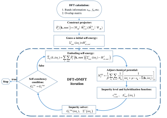
Figure 1: Flow diagram of the major steps in our DFT+DMFT implementation.

In this section, we will explain step by step our DFT+DMFT calculation procedure, according to the workflow outlined in the flow diagram depicted in Fig. 1.

Step 1. The DFT+DMFT calculation starts from well-converged DFT band structures. To get high-quality KS orbitals $|\Psi_{i\bf{k}}\rangle$, a dense ${\bf k}$-point mesh is usually needed.

Step 2. With $|\Psi_{i\bf{k}}\rangle$, the projector defined in Eq. (20) can be straightforwardly constructed. To this end, the most localized $d$ or $f$ orbital of the correlated atoms in the NAO basis set is used to construct $|W_{I,m}^{0}\rangle$.

Step 3. In the DFT+DMFT iteration loop, the frequency-dependent self-energy $\Sigma(i\omega_{n})$ is determined by the impurity solver at each iteration step. To start with, the initial self-energy is set to be equal to the double-counting term, i.e., $\bar{\Sigma}_{ij}(\mathbf{k},i\omega_{n})=0$. Here the following choice of the double-counting term

$$H_{\mathrm{dc},mm^{\prime}}^{I,\sigma}=\left[U(n_{I}-1/2)-1/2J(n_{I}-1)\right]\delta_{mm^{\prime}}$$ (23)

is used. Here $n_{I}$ is the total number of correlated electrons associated with the correlated atom $I$ and is fixed during the DMFT cycles. In the spirit of reducing the necessity of introducing additional empirical parameters, $n_{I}$ is given by projecting the KS orbitals in the subset $\mathcal{C}$ to the local subspace as

$$n_{I}=\sum_{m}\sum_{\mathbf{k}}\frac{1}{N_{\mathbf{k}}}\sum_{i\in\mathbf{C}}f_{i\mathbf{k}}\tilde{P}_{ii}^{I}\left(\mathbf{k},mm\right)\,,$$ (24)

where $f_{i\mathbf{k}}$ is the occupation number of KS orbital $\Psi_{i\mathbf{k}}$. This double-counting scheme is similar to the so-called fixed double-counting [22, 64] scheme, which is considered to be able to improve the stability of DFT+DMFT self-consistency loop [64] by fixing the value of $n_{I}$. The difference is that the nominal number of strongly correlated electrons is specified manually in the fixed double-counting scheme, whereas in our case this number is determined using Eq. (24).

Step 4. Using the projector constructed in Step 2, we embed (upfold) the self-energy back to the selected KS space subset $\mathcal{C}$, which is expressed as

$$\bar{\Sigma}_{ij}(\mathbf{k},i\omega_{n})= \sum_{I}\sum_{mm^{\prime}}\tilde{P}_{ij}^{I}\left(\mathbf{k},mm^{\prime}\right)$$ (25)

$$\left(\Sigma_{mm^{\prime}}^{I}(i\omega_{n})-H_{\mathrm{dc},mm^{\prime}}^{I}\right).$$

Step 5. During the DFT+DMFT self-consistency iteration, the electronic chemical potential needs to be adjusted according to the newly obtained self-energy at each iteration, to keep the number of electrons hosted by KS bands in $\mathcal{C}$

$$N_{\mathcal{C}}^{\mathrm{KS}}=\sum_{\mathbf{k},i\in\mathcal{C}}\frac{1}{N_{\mathbf{k}}}f_{i\mathbf{k}}$$ (26)

conserved. Within the DMFT cycle, this condition means that

$$N_{\mathcal{C}}^{\mathrm{KS}}= \frac{1}{\beta}\sum_{\omega_{n}}\sum_{\mathbf{k},i\in\mathcal{C}}\frac{1}{N_{\mathbf{k}}}$$ (27)

$$\left[\frac{1}{i\omega_{n}+\mu-\epsilon_{\mathbf{k}}-\bar{\Sigma}(\mathbf{k},i\omega_{n})}\right]_{ii}\,,$$

where $\beta$ is again the inverse temperature $1/{k_{B}T}$. The summation of imaginary frequency $\omega_{n}$ should run from negative infinity to positive infinity. However, in realistic calculations, to save computational cost, the explicit summation over Matsubara frequency points is only carried within a frequency window $[-\omega_{N},\omega_{N}]$, where the contribution from the frequency points outside the window is treated approximately. This is enabled by making use of the asymptotic behavior of the self-energy, i.e., $\lim_{n\to\infty}\bar{\Sigma}_{ii}(\mathbf{k},i\omega_{n})=\bar{\Sigma}_{ii}(\mathbf{k},\infty)$, where $\bar{\Sigma}_{ii}(\mathbf{k},\infty)$ is a real value. Then the Eq. (27) is approximated by

$$N_{\mathcal{C}}^{\mathrm{KS}}= \frac{1}{\beta}\sum_{\mathbf{k},i\in\mathcal{C}}\frac{1}{N_{\mathbf{k}}}\left\{\sum_{\omega_{n}=-\omega_{N}}^{\omega_{N}}\right.$$ (28)

$$\left(\left[\frac{1}{i\omega_{n}+\mu-\epsilon_{\mathbf{k}}-\bar{\Sigma}(\mathbf{k},i\omega_{n})}\right]_{ii}\right.$$

$$\left.-\left[\frac{1}{i\omega_{n}+\mu-\epsilon_{k}-\bar{\Sigma}(\mathbf{k},\infty)}\right]_{ii}\right)$$

$$\left.+\frac{1}{1+e^{\beta(\epsilon_{i\mathbf{k}}+\bar{\Sigma}_{ii}(\mathbf{k},\infty)-\mu)}}\right\}.$$

When the chosen cutoff Matsubara frequency $\omega_{N}$ is high enough so that the asymptotic behavior of the self-energy is correct, this approximation is of good accuracy.

Step 6. As all information is secured, the local interacting Green function is constructed from Eq. (17), where, of course, the renormalized projector Eq. (20) is used. Under the DFT+DMFT self-consistency condition, Eq. (1) and (8), the matrices of the impurity level and hybridization function are determined by

$${\cal E}_{I,mm^{\prime}}^{imp}=-H_{dc,mm^{\prime}}^{I}+\sum_{\mathbf{k},i\in\mathcal{C}}\frac{1}{N_{\mathbf{k}}}\tilde{P}_{ij}^{I}\left(\mathbf{k},mm^{\prime}\right)\varepsilon_{i\mathbf{k}}$$ (29)

and

$$\Delta_{mm\prime}^{I}\left(i\omega_{n}\right)= (i\omega_{n}+\mu)\delta_{mm^{\prime}}-{\cal E}^{imp}_{I,mm^{\prime}}$$ (30)

$$-\Sigma_{mm^{\prime}}^{I}\left(i\omega_{n}\right)-[G^{loc}]^{-1}_{I,mm^{\prime}}.$$

For some CT-HYB impurity solver, the imaginary time hybridization function is needed.

Step 7. Solve the impurity problem with the determined $\mu$, ${\cal E}_{I}^{imp}$, $\Delta^{I}\left(i\omega_{n}\right)$ and the given on-site Coulomb interaction through the impurity solver to obtain the new self-energy and impurity Green function. In this paper, we use the Kanamori [65, 66] form Coulomb interaction in which only the density-density term is included, so there are no sign problem in our CTQMC calculations.

Step 8. Check whether the self-consistency is reached. If the self-consistency is reached, stop the DFT+DMFT calcution, else return to Step 4.

III Results and discussion

III.1 d-electron systems

We first benchmark our DFT+DMFT implementation on three prototypical strongly correlated d-electron systems – SrVO₃, NiO, and MnO. For the DFT part, we carried out GGA calculations using two NAO-based code packages – FHI-aims [37] and ABACUS [38]. In FHI-aims, the default tight tier 1 basis set is used for V, Ni, Mn, O, and Sr atoms, and the corresponding cutoff radii of the basis functions are $6.0\text{\,}\mathrm{\SIUnitSymbolAngstrom}$, $6.0\text{\,}\mathrm{\SIUnitSymbolAngstrom}$, $6.0\text{\,}\mathrm{\SIUnitSymbolAngstrom}$, $6.0\text{\,}\mathrm{\SIUnitSymbolAngstrom}$, and $8.0\text{\,}\mathrm{\SIUnitSymbolAngstrom}$, respectively. In ABACUS we use the SG15 optimized norm-conserving Vanderbilt (ONCV) multi-projector pseudo-potentials [67, 68, 69] and the corresponding optimized double-$\zeta$ plus polarization (DZP) atomic basis sets, which comprise $4s2p2d1f$ basis functions with a cutoff radius of $9.0\text{\,}\mathrm{B}\mathrm{o}\mathrm{h}\mathrm{r}$ for transition metal atoms and $2s2p1d$ basis functions with cutoff radii of $7.0\text{\,}\mathrm{B}\mathrm{o}\mathrm{h}\mathrm{r}$ for O atoms and $10.0\text{\,}\mathrm{B}\mathrm{o}\mathrm{h}\mathrm{r}$ for Sr atoms. In all DFT calculations, the Perdew-Burke-Ernzerhof (PBE) GGA exchange-correlation functional was used [70]. As for the DMFT part, we employed three different CT-HYB impurity solvers to solve the single-site impurity problem. These are PACS developed by one of the present authors Gang Li, iQIST developed by Huang et al. [72, 73, 74], and the one used in eDMFT [30] developed by Haule at Rutgers University [62, 75], which is referred to as “Rutgers” below in this paper.

III.1.1 SrVO₃

SrVO₃ has a simple cubic perovskite structure without magnetism. DFT fails to reproduce the upper and lower Hubbard bands observed in experiments, and this calls for advanced theoretical and computational techniques [8]. In the past, this material has been extensively studied both theoretically and experimentally [25, 76, 77, 78, 79, 80, 81, 82], which provides abundant reference results. Therefore, SrVO₃ is an ideal test example for DFT+DMFT implementations [24, 26, 27, 66, 46]. The V⁴⁺ cation with only one 3d electron is located in the center of the octahedron formed by its six surrouding axial O^2- ligand anions. In the presence of an octahedral crystal field, the five degenerate d orbitals split into two subsets: Three-fold degenerate t_2g orbitals (i.e., $d_{xy}$, $d_{yz}$ and $d_{xz}$), and two-fold degenerate e_g orbitals (i.e., $d_{z^{2}}$ and $d_{x^{2}-y^{2}}$). The only one 3d electron of V⁴⁺ occupies the lower-energy t_2g orbitals with the higher-energy e_g orbitals being empty. As a common practice, we only consider three degenerate t_2g orbitals in our DFT+DMFT calculation.

In DFT calculations, we use 11$\times$11$\times$11 ${\bf k}$-point mesh generated by the Monkhorst-Pack method [83]. The Hubbard U and Hund J parameters are set to be $4.0\text{\,}\mathrm{eV}$ and $0.65\text{\,}\mathrm{eV}$, respectively, following the choice in the literature [26, 27, 46]. The DMFT calculation is carried out at a temperature of $300\text{\,}\mathrm{K}$. DFT calculations give a group of bands around the Fermi level with substantial 3d characterizes, which are well separated from other bands [26, 27]. We enclose the six (twelve if spin degree of freedom is taken into account) bands crossing the Fermi level in the subset of KS bands $\mathcal{C}$.

Figure 2: The single-particle energy spectral function of SrVO₃ 3d electrons given from direct analytical continuation of the impurity Green function. The results presented in the six panels are obtained by six computational schemes combining two DFT codes – FHI-aims (upper panels) and ABACUS (lower panels) and three different impurity solvers – PACS (left panels), iQIST (middle panels), and Rutgers (right panels).

One of the powerful strengths of Green-function based DFT+DMFT approach is that it can deliver physically meaningful single particle excitation spectral functions, as given by the the imaginary part of Green function. Such spectral functions can be directly measured by photoemission and/or inverse photoemission experiments. In Fig. 2, the spectral functions of 3d electrons of SrVO₃ calculated by combining two NAO-based DFT packages – FHI-aims and ABACUS, and three impurity solvers – PACS, iQIST and Rutgers are presented. Despite the considerable differences underlying the implementations of the DFT codes, as well as the DMFT impurity solvers, the calculated spectral functions are remarkably similar. Most importantly, they all successfully reproduce the typical three-peak structure: A quasi-particle band located at the Fermi level with the lower and upper Hubbard bands on the two sides, arising from the strong electron correlations which traditional LDA and GGA fail to capture. The main features of the spectral functions given by our DFT+DMFT calculations are in good agreement with previous theoretical results except for some small details such as the exact peak positions and intensities [78, 25, 79, 24, 76, 26, 27, 66, 46]. Our results also correctly describe the strong particle-hole asymmetry of the lower and upper Hubbard band as the intensity of the occupied lower Hubbard band is much smaller than the empty upper Hubbard band. This is the consequence that the V⁴⁺, with only one 3d electron, is far away from half-filling.

Similar to previous DFT+DMFT studies [25, 79, 24, 76, 26, 27, 66, 46], our spectral function results are in excellent agreement with the experimental photoemission spectrum [78]. The first main feature lies in the reproduction of the lower Hubbard band at around $-2.0\text{\,}\mathrm{eV}$, which is the manifestation of the strong correlation among 3d electrons. The second feature, in quantitative agreement with experiment, is that the lower Hubbard band vanishes at $\sim$-1.0\text{\,}\mathrm{eV}$$, and then the quasiparticle band starts to rise sharply.

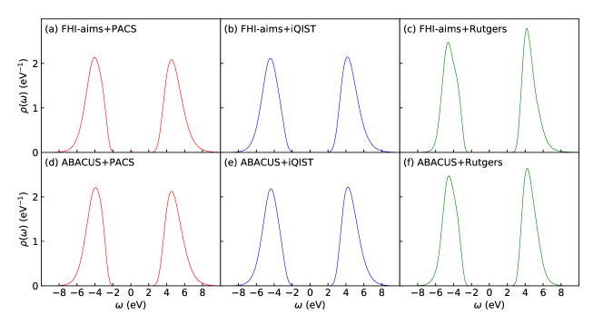
Figure 3: The spectral function of MnO 3d electrons obtained from direct analytical continuation of the impurity Green function. Similar to Fig. 2, results presented in the six panels are obtained by two different DFT codes combined with three different impurity solvers. Each panel is labelled by the specific combination.

III.1.2 MnO and NiO

Next we test our DFT+DMFT scheme on the late transition metal oxides MnO and NiO. Both MnO and NiO crystallize in face-centered cubic (FCC) NaCl-type structures where 3d orbitals are split into threefold degenerate $t_{2g}$ and twofold degenerate $e_{g}$ orbitals as in the SrVO₃ case. In the MnO system, we adopt the parameters of U$=$$5.0\text{\,}\mathrm{eV}$, J$=$$1.0\text{\,}\mathrm{eV}$, and the temperature $T=$$300\text{\,}\mathrm{K}$. For MnO, the KS bands within the energy window of [$-3.0\text{\,}\mathrm{eV}$, $3.0\text{\,}\mathrm{eV}$] are included in the subset $\mathcal{C}$. For NiO, another set of parameters with the temperature of $1160\text{\,}\mathrm{K}$, U of $8.0\text{\,}\mathrm{eV}$ and J of $1.0\text{\,}\mathrm{eV}$ [6, 84, 85, 46] is used. The energy window enclosing the subset of KS bands $\mathcal{C}$ is chosen to be [$-2.0\text{\,}\mathrm{eV}$, $1.0\text{\,}\mathrm{eV}$].

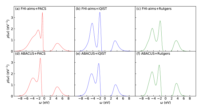
Figure 4: The single-particle spectral function of NiO 3d electron calculated from direct analytical continuation of the impurity Green function. The meaning of the six panels is same as Fig. 2 and 3.

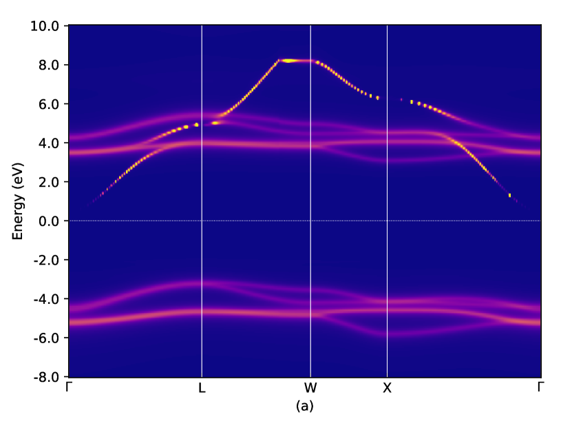
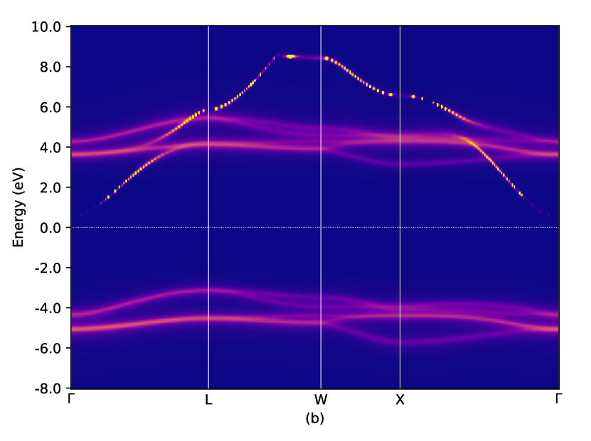
Figure 5: The ${\bf k}$-resolved spectral function $A(\mathbf{k},\omega)$ of MnO, obtained by (a) FHI-aims+Rutgers and (b) ABACUS+Rutgers, respectively.

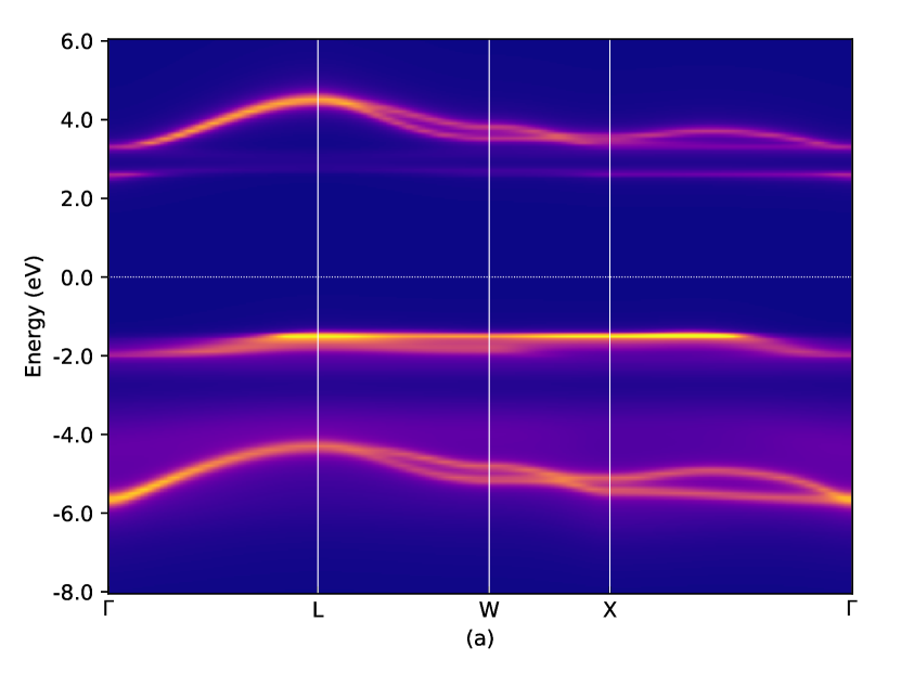
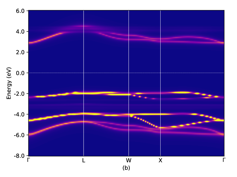
Figure 6: The k-resolved spectral function $A(\mathbf{k},\omega)$ of NiO, obtained by (a) FHI-aims+Rutgers and (b) ABACUS+Rutgers, respectively.

MnO and NiO are classical examples that clearly demonstrate the failure of traditional band theory, e.g., LDA and GGA. LDA and GGA predict MnO and NiO to be metallic while they are wide-gap insulators experimentally. Even though a gap will appear if the spin-symmetry-broken antiferromagnetic state is considered, the calculated gap is however still one order of magnitude smaller than the experimental values. By merging the Hubbard model and ab-initio DFT, static DFT+U [6, 20, 21] and the more advanced dynamical DFT+DMFT [84, 85] successfully open the gaps in those prototypical transitional metal oxides. Then obtained band gaps are in quantitative agreement with experiments, if proper parameters are used.

We then apply our DFT+DMFT implementation to both MnO and NiO, and the obtained spectral functions are presented in Fig. 3 and Fig. 4, respectively. Again in each figure, we present six panels containing results obtained by combining two NAO-based DFT codes and three DMFT impurity solvers. The most prominent feature in the DFT+DMFT spectra of both MnO and NiO is that a sizeable gap is opened up, arising apparently from the strong Coulomb interactions whose effect is properly captured by DMFT. One can further see from Fig. 3 that the intensity of the lower and upper Hubbard band of Mn 3d electrons are nearly the same. This result is consistent with the nominally half-filling 3d orbitals of Mn given by chemical analysis, which is confirmed by the fact that the number of 3d electrons of Mn given by $n=-\sum_{m}G^{imp}_{mm}(\beta)$ is 5. Similar to the SrVO₃ case, the results presented in all six panels are very close, except that the peaks given by the Rutgers impurity solver is slightly more pronounced.

For NiO, the number of nominal $3d$ electrons is approximately 8, and DFT+DMFT calculations lead to a splitting of the $3d$ bands, with fully occupied $t_{2g}$ orbitals and half-filled $e_{g}$ orbitals. Our results in general agree well with previous DFT+DMFT results reported in the literature [84, 85]. However, Fig. 4 also reveals that both the DFT codes and the impurity solvers have certain influence on the obtained DFT+DMFT energy spectra. Although there are no qualitative differences, the shape and width of the left peak, and the depth of the dip between the first and middle peaks show noticeable quantitative differences. It is not entirely clear to us yet what factors caused such differences. We note that, however, NiO is a prototypical charge transfer insulator [86], and the competition between the strong Coulomb interactions among the Ni $3d$ electrons and the hybridization between the Ni $3d$ and O $2p$ electrons governs its underlying physics. Thus a complete DFT+DMFT treatment of NiO should also include O $2p$ electrons in the game. With the O $2p$ excluded, the DFT+DMFT calculations are probably more sensitive to the details in the band structures and numerical techniques behind the impurity solvers.

Figure 3 and 4 only contain the spectral information of 3d electrons. Our DFT+DMFT implementation also allows for calculating the ${\bf k}$-resolved spectral function in the KS orbital space, as determined by

$$A(\mathbf{k},\omega)=-\frac{1}{\pi}\sum_{i\in\mathcal{C}}\operatorname{Im}\left[(\omega+\mu-\epsilon({\mathbf{k}}))I-\bar{\Sigma}(\mathbf{k},\omega)\right]^{-1}_{ii},$$ (31)

where the real-frequency self-energy is evaluated by analytical continuation of the imaginary frequency-self-energy through the maximum entropy formalism in Ref. [87]. The corresponding results for MnO and NiO are presented in Figs. 5 and 6, respectively. Now for simplicity only results obtained using the two DFT codes combined with the Rutgers impurity solver are presented. The agreement between our theoretical gaps and experimental gaps [88, 89, 90] is rather satisfactory. The two ${\bf k}$-resolved spectral functions of MnO is nearly identical whereas again noticeable differences, in particular regarding the spectral weights of certain bands, exist for NiO. Nevertheless the main features, e.g., the energy positions and dispersion of the bands, are reasonably similar in Fig. 6(a) and 6(b).

NiO has been extensively studied experimentally, and reliable experimental photoemission spectra are available. In Fig. 7, we directly compare our DFT+DMFT spectrum of NiO with the experimental spectrum of Sawatzky and Allen [89] measured by x-ray-photoemission (XPS) and bremsstrahlung-isochromat-spectroscopy (BIS) techniques. Again, the two sets of theoretical spectra are obtained using FHI-aims and ABACUS codes interfaced with the Rutgers impurity solver, respectively. For the spectrum below the Fermi level, corresponding to the (negative of) energy cost for removing a particle from the occupied levels, we reproduce the sharp peak around $-2.0\text{\,}\mathrm{eV}$ and a local minimum at $-3.0\text{\,}\mathrm{eV}$ given by XPS. For the spectrum above the Fermi level, corresponding to the (negative of) energy cost for adding a particle to the system, our curves match perfectly with the BIS result. Although small deviations of the shoulder peak at approximately $-3.5\text{\,}\mathrm{eV}$ are visible, our DFT+DMFT spectrum, in general, agrees well with previous theoretical work [84] and the experiment data[89].

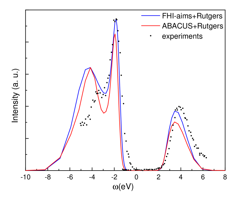
Figure 7: Comparison of theoretical and experimental spectral functions of NiO. The theoretical results are given by the imaginary part of the impurity Green function on the real frequency axis, analytically continued from the Matsubara impurity Green function. The experimental data are obtained from XPS+BIS measurements, taken from Ref. [89].

In ABACUS, the pseudopotential method is used and only the valence electrons are explicitly included. Furthermore, as given in the beginning of this section, the spatial cutoffs of NAOs used in ABACUS are much smaller than those used in FHI-aims. By contrast, in FHI-aims full potential is used with all electrons being included in DFT calculations. Although these two NAO schemes are rather different, we get nearly identical DFT+DMFT results of SrVO₃ and MnO and reasonably similar results for NiO. It proves the efficacy and robustness of our DFT+DMFT formalism and implementation. We expect that the DFT+DMFT formalism presented in this paper should work for other NAO-based DFT codes as well.

III.2 f-electron systems

The f-electron systems, including 4f lanthanides and 5f actinides, are an important class of strongly correlated materials characterized by partially filled f-type orbitals. These systems exhibit a variety of exotic phenomena, such as the heavy-fermion behavior, metal-insulator transition, Kondo physics, volume collapses accompanying phase transitions, etc. It has been generally accepted that traditional DFT calculations based on static mean-field-type approximations such as LDA and GGAs do not provide adequate accuracy for describing these physical scenarios. DFT+DMFT has proved to be a powerful approach to tackle these systems and achieved remarkable successes in the last two decades. In this section we test our DFT+DMFT implementation on several typical f-electron systems, including 4f systems like $\alpha$ and $\gamma$ cerium (Ce) metal and Ce₂O₃, and 5f systems like PuO₂ and Pu₂O₃.

DFT calculations are carried out using FHI-aims with the default tight tier1 basis sets. For these basis sets, the cutoff radii of Ce, Pu, and O elements are $7\text{\,}\mathrm{\SIUnitSymbolAngstrom}$, $6.0\text{\,}\mathrm{\SIUnitSymbolAngstrom}$, and $6.0\text{\,}\mathrm{\SIUnitSymbolAngstrom}$, respectively. Analogous to the case of $3d$-electron systems, the GGA-PBE functional [70] is used in the DFT calculations and 11$\times$11$\times$11 Monkhorst-Pack ${\bf k}$-point mesh [83] is used for Brillouin-zone integration, which is deemed dense enough to obtain accurate DFT band structures. Unlike the practice in previous sections where results obtained using three DMFT impurity solvers are shown for comparison, here for simplicity only the results obtained using the Rutgers solver will be presented.

III.2.1 Ce metal

Despite its simple FCC structure and the fact that only one 4f valence electron is present per Ce atom, Ce exhibits spectacular physical properties, which has attracted considerable research interest over the last forty decades [91, 92, 93, 94, 95, 96, 97, 66, 98, 99]. At low temperature and ambient pressure, Ce crystalizes in the $\alpha$ phase (smaller volume), where the system is paramagnetic and shows Pauli-like magnetic susceptibility without forming local magnetic moments. At high temperature, Ce transforms into the $\gamma$ phase (larger volume), which instead carries local magnetic moments and exhibits Curie-Weiss behavior of magnetic susceptibility. When increasing pressure or decreasing temperature, Ce undergoes the famous isostructural $\gamma$-$\alpha$ phase transition accompanied by a 14% volume collapse and a drastic change of magnetic properties [93, 94, 95, 96, 97, 66, 98, 99]. A theoretical understanding of this behavior poses a great challenge to condensed matter physics and has motivated lots of experimental and theoretical investigations. From the perspective of first-principles computations, standard DFT calculations are unable to give a proper description of this phase transition, and the approaches going beyond conventional DFT are required.

In this paper, the crystal structures of $\alpha$ and $\gamma$ Ce phases are discerned by different volumes, i.e., $29\text{\,}\mathrm{\SIUnitSymbolAngstrom}$³ for $\alpha$ and $34\text{\,}\mathrm{\SIUnitSymbolAngstrom}$³ for $\gamma$ phase, respectively, which covers the volume ranges during the $\alpha$-$\gamma$ transition [94]. The chosen energy window for KS subset $\mathcal{C}$ is [$-5.0\text{\,}\mathrm{eV}$, $5.0\text{\,}\mathrm{eV}$]. The Coulomb interaction parameter U given by constrained DFT is $6.0\text{\,}\mathrm{eV}$ [66, 98]. Here we used the value of U of $6.0\text{\,}\mathrm{eV}$ and Hund parameter J of $0.5\text{\,}\mathrm{eV}$ [96, 98]. DFT+DMFT calculations are done at the temperature of $800\text{\,}\mathrm{K}$.

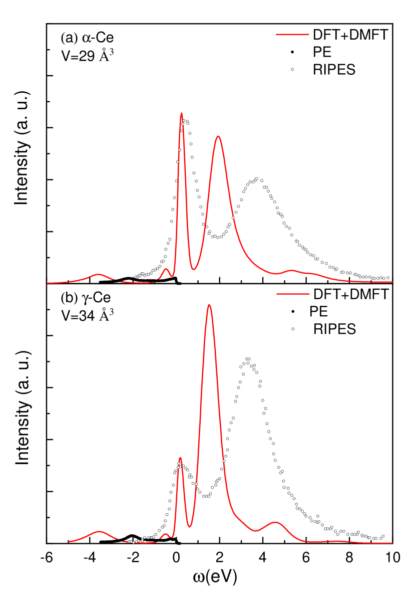
Figure 8: Comparison of theoretical and experimental spectral functions of $\alpha$ and $\gamma$ Ce. The DFT+DMFT calculation is carried out by FHI-aims interfaced with the Rutgers impurity solver and the corresponding spectral results are given by direct analytical continuation of the impurity Green function. The resonant inverse photoemission spectroscopies (RIPES) are taken from Ref. [91], and the photoemission (PE) spectra are taken from Ref. [92].

Our DFT+DMFT spectra for Ce are shown in Fig. 8. First of all, the energy spectra of both phases show the characteristic three-peak structures of strongly correlated metals. One can also see that, going from the $\alpha$ phase to the $\gamma$ phase, the central quasiparticle peak gets substantially suppressed, and its spectral weights transfer to the lower and upper Hubbard bands . Such results are in agreement with experimental observations [91, 92] and previous DFT+DMFT calculations for Ce [94, 95, 96, 98]. The relative strengths of the quasi-particle peak and the upper Hubbard peak of both $\alpha$ and $\gamma$ phases are also captured qualitatively. However, a direct comparison of the calculated spectra with the experimental spectra reveals that the energy separation between the quasi-particle peak and upper Hubbard band is underestimated in our calculations, while that between the lower Hubbard band and quasi-particle peak is overestimated. Compared to previous DFT+DMFT calculations, the location of the lower Hubbard peak of our results is close to that reported in the literature [94, 98] where the maximum of lower Hubbard peaks is around -4.0$\sim$$-3.0\text{\,}\mathrm{eV}$. Concerning the energy positions of the upper Hubbard band, we found that the results reported in the literature also vary quite a bit, with those reported in Ref. [98] agreeing best with experiment. Our results are close to those reported in Ref. [96], where the upper Hubbard peaks are located at around $2.5\text{\,}\mathrm{eV}$. In general, our DFT+DMFT spectrums are in quantitative agreement with experimental and previous theoretical results. The discrepancies between our results and experimental and previous theoretical results indicate that details of the DFT calculations, the definition of the projector, as well as the numerical implementation of the impurity solvers will still have appreciable influence on the outcomes of DFT+DMFT calculations. Further investigations along these lines are still needed.

III.2.2 Ce₂O₃

Ce₂O₃ is a Mott insulator with a gap of about $2.4\text{\,}\mathrm{eV}$ [100, 22] arising from the strong correlation among 4f electrons. This system has been calculated using a variety of approaches such as DFT+U, GW [101], and DFT+DMFT [22, 28]. Ce₂O₃ crystalizes in the hexagonal lattice with space group $P\bar{3}m1$. The experimental lattice parameters $a=b=$3.891\text{\,}\mathrm{\SIUnitSymbolAngstrom}$$, $c=$6.059\text{\,}\mathrm{\SIUnitSymbolAngstrom}$$ [102] are used in our calculations. The energy window for KS subset $\mathcal{C}$ is [$-3.0\text{\,}\mathrm{eV}$, $2.0\text{\,}\mathrm{eV}$]. Constrained DFT calculation predicted the parameter U varying from 5.5 to $8.0\text{\,}\mathrm{eV}$, and we adopt U as $6.5\text{\,}\mathrm{eV}$ and J as $0.5\text{\,}\mathrm{eV}$. The temperature is set to be $300\text{\,}\mathrm{K}$.

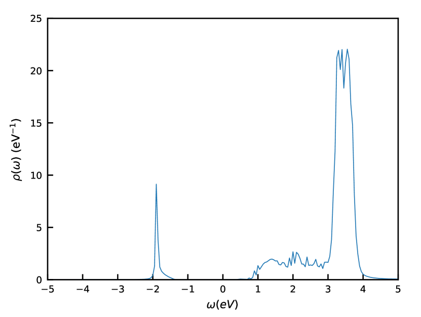
Figure 9: DOS of Ce₂O₃. The DFT+DMFT calculation is carried out by combination FHI-aims and impurity solver Rutgers.

Here we calculate the total density of states (TDOS) of Ce₂O₃ through

$$\rho(\omega)=\frac{1}{N_{\mathbf{k}}}\sum_{\mathbf{k}}A(\mathbf{k},\omega),$$ (32)

where $A(\mathbf{k},\omega)$ is defined in Eq. (31). The result is shown in Fig. 9, our DFT+DMFT calculation gives a band gap of about $2.5\text{\,}\mathrm{eV}$, which agrees well with the experimental and previous theoretical results [100, 22, 101, 28]. For example, all predict that the lower Hubbard peaks are sharp and narrow whereas the upper Hubbard peaks are strong and wide. The interesting feature about the upper Hubbard part is that it emerges as a low plateau between 1 and 3 eV above the Fermi level, continued by a pronounced peak between 3 and 4 eV. Note that the peaks mainly composed of O p bands sitting below the lower Hubbard peaks does not show up here due to the fact that those O p characteristic bands are not included in the subset $\mathcal{C}$ in the DFT+DMFT calculations whereas they are retained in Refs. [22, 101, 28].

III.2.3 Pu₂O₃ and PuO₂

Plutonium (Pu)-based oxides such as Pu₂O₃ and PuO₂ are essential for the fuel components in current nuclear reactors, as well as transmutation of the minor actinides from spent nuclear fuels [103, 104]. A clear understanding of the physio-chemical properties of plutonium-based oxides is of key importance for the safe operation and development of nuclear reactor systems and nuclear waste reprocessing [105, 106], and the correct description of the oxidation and reduction processes [107, 108]. The physical, chemical, and thermodynamical properties of Pu-based oxides such as the chemical bonding and electronic structure are intimately related to the states of strongly correlated 5f electrons. Conversely, the relative tendency of delocalization versus localization of strongly correlated 5f electrons is extremely sensitive to the physical and chemical environment of the Pu atom [109]. The description of complicated behaviors of 5f electrons, e.g., whether they are settled in the delocalized or localized states, or in the intermediate regime, is out of the reach of standard DFT. In contrast, DFT+DMFT is becoming a promising approach that facilitates an in-depth understanding of this type of materials.

In this paper, we look at two plutonium oxides, i.e., Pu₂O₃ in its $\beta$ phase [110] (simply called Pu₂O₃ below) and PuO₂ [111] with our DFT+DMFT implementation. We use the Hubbard parameter U of $4.0\text{\,}\mathrm{eV}$ and the Hund parameter J of $0.5\text{\,}\mathrm{eV}$ for Pu₂O₃. As for PuO₂, U and J are chosen to be $5.0\text{\,}\mathrm{eV}$ and $0.6\text{\,}\mathrm{eV}$. The electronic temperatures for both systems are set at $300\text{\,}\mathrm{K}$. The chosen energy windows for the KS subsets $\mathcal{C}$ are [$-3.0\text{\,}\mathrm{eV}$, $2.0\text{\,}\mathrm{eV}$] for Pu₂O₃, and [$-3.0\text{\,}\mathrm{eV}$, $3.0\text{\,}\mathrm{eV}$] for PuO₂.

We calculated DFT+DMFT TDOS of Pu₂O₃ through the method introduced in the case of Ce₂O₃. The TDOS here contains contributions from both the correlated orbitals and the rest (here $spd$) orbitals. The projected density of states (PDOS) belonging to correlated ($5f$) orbitals, is evaluated by

$$\rho_{f}(\omega)= \sum_{m}\frac{1}{N_{\mathbf{k}}}\sum_{\mathbf{k}}-\frac{1}{\pi}\operatorname{Im}\left\{\tilde{P}^{I}_{ij}(\bm{k},mm)\right.$$ (33)

$$\left.\left[(\omega+\mu-\epsilon({\mathbf{k}}))I-\bar{\Sigma}(\mathbf{k},\omega)\right]^{-1}_{ij}\right\}\,$$

whereas the PDOS for the $spd$ orbitals is obtained by taking the difference between the TDOS and $\rho_{f}(\omega)$. The results are depicted in Fig. 10. Figure 10 indicates that the band gap of Pu₂O₃ as determined by DFT+DMFT is about $1.7\text{\,}\mathrm{eV}$, which is in good agreement with the experimental bands gap of $1.8\text{\,}\mathrm{eV}$ [112, 28]. Additionally, the occupation analysis yields an average occupation number n_f=5.0 for Pu 5f electrons through $n=-\sum_{m}G^{imp}_{mm}(\beta)$, which is consistent with the chemical environment of Pu³⁺ in Pu₂O₃.

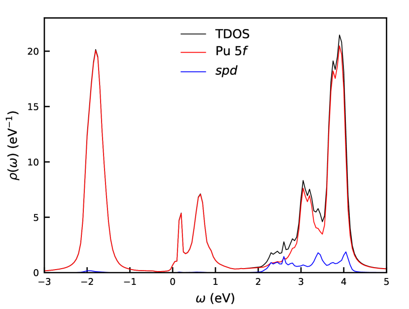
Figure 10: TDOS and PDOS of Pu₂O₃. The TDOS is given by Eq. (32). The PDOS of Pu 5f electrons is evaluated through Eq. (33). The PDOS for spd electrons is obtained by subtracting the PDOS of Pu 5f electrons from the TDOS. The DFT+DMFT calculation is carried out by combining FHI-aims and the Rutgers impurity solver.

In Fig. 11, the DFT+DMFT TDOS of PuO₂ is plotted. The bands gap is predicted to be about $2.5\text{\,}\mathrm{eV}$, which is in good agreement with previous theoretical work [113] and the experimental band gap of $2.8\text{\,}\mathrm{eV}$ [114]. In PuO₂, the peak of occupied Pu 5f electrons is noticeably sharper than that of Pu₂O₃, which indicates that the Pu 5f electrons in PuO₂ are likely more localized than the case of Pu₂O₃. This localization picture is in agreement with the bigger gaps in PuO₂. The occupation analysis gives an average occupation number of n_f=4.0 for Pu 5f electrons, which agrees with the chemical state of Pu⁴⁺ in PuO₂.

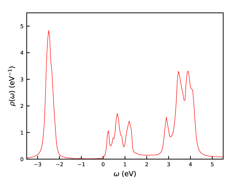
Figure 11: DFT+DMFT TDOS of PuO₂. The DFT+DMFT calculation is carried out by a combination FHI-aims and the Rutgers impurity solver.

IV Summary

In summary, we developed and implemented a formalism that allows us to carry out DFT+DMFT calculations within the NAO basis set framework. For transition metal compounds and $f$-electron systems, the most localized $d$ or $f$-type NAO is used to define the local correlated subspace. Such a choice is physically intuitive and implementationally convenient for NAO basis sets. Following what is usually done in the literature, only a subset of the KS bands $\mathcal{C}$ out of the full KS space around the Fermi energy, which hosts the majority of electrons with strong correlations, are enclosed in the definition of the projector. Our projector scheme is mathematically equivalent to the projective-Wannier-function approach adopted in Ref. [24]. We implemented such a DFT+DMFT formalism by interfacing two NAO-based DFT codes, i.e., FHI-aims [37] and ABACUS [38] with three DMFT quantum impurity solvers, i.e., PACS, iQIST [72, 73, 74], and the Rutgers impurity solver [30, 62, 75]. In particular, interfacing with the all-electron FHI-aims code allows one to study all types of strongly correlated materials over the periodic table.

Our DFT+DMFT formalism and implementation are testified for three typical series of strongly correlated materials, namely the 3d transitional metal compounds SrVO₃, MnO and NiO, 4f materials including the Ce metal and Ce₂O₃, as well as the 5f actinides Pu₂O₃ and PuO₂. For SrVO₃ and MnO, our calculated one-electron removal and addition spectra are in good agreement with previously reported DFT+DMFT results and experimental data. Furthermore, the calculated results are rather robust against the use of different DFT codes or different impurity solvers. For NiO, the obtained DFT+DMFT results show noticeable dependence on the chosen DFT codes and/or impurity solvers, although the key spectroscopic features are captured by all calculations. For $f$-electron systems, the characteristic three-peak structures are obtained for the Ce metal, whereas for the correlated insulators, the obtained DFT+DMFT band gaps are in good agreement with experiments. However, there remain issues calling for further investigations, like the energy separation of the quasiparticle peak and the upper Hubbard band for the Ce metal.

Admittedly, our scheme is still in its infancy, and at the quantitative level there are still issue to be sorted out. Further improvement would be necessary for more reliable descriptions of charge-transfer-type Mott insulators, and the intricate lanthanides and actinides. However, we consider that our attempt of developing an infrastructure that merge NAO-based DFT codes and DMFT-based techniques is rather rewarding. This will not only enable standard DFT+DMFT calculations within the NAO basis set framework, but also paves the way for developing more advanced schemes by combining beyond-DFT approaches like hybrid functionals [40, 115, 41] or $GW$ [42], recently available in NAO-based DFT codes, with the DMFT machinery.

- [1] Paul R. C. Kent and Gabriel Kotliar. Toward a predictive theory of correlated materials. Science, 361(6400):348–354, jul 2018.
- [2] Arpita Paul and Turan Birol. Applications of DFT+DMFT in Materials Science. Annu. Rev. Mater. Res., 49(1):31–52, jul 2019.
- [3] Ran Adler, Chang-Jong Kang, Chuck-Hou Yee, and Gabriel Kotliar. Correlated materials design: prospects and challenges. Reports Prog. Phys., 82(1):012504, jan 2019.
- [4] P. Hohenberg and W. Kohn. Inhomogeneous electron gas. Phys. Rev., 136:B864–B871, 1964.
- [5] W. Kohn and L. J. Sham. Self-Consistent Equations Including Exchange and Correlation Effects. Phys. Rev., 140(4A):A1133–A1138, 1965.
- [6] Vi Vi Anisimov, J. Zaanen, and O. K. Andersen. Band theory and Mott insulators: Hubbard U instead of Stoner I. Phys Rev B: Condens Matter, 44(3):943–954, 1991.
- [7] Antoine Georges, Gabriel Kotliar, Werner Krauth, and Marcelo J. Rozenberg. Dynamical mean-field theory of strongly correlated fermion systems and the limit of infinite dimensions. Rev. Mod. Phys., 68(1):13–125, 1996.
- [8] G. Kotliar, S. Y. Savrasov, K. Haule, V. S. Oudovenko, O. Parcollet, and C. A. Marianetti. Electronic structure calculations with dynamical mean-field theory. Rev. Mod. Phys., 78(3):865–951, 2006.
- [9] K. Held. Electronic structure calculations using dynamical mean field theory. Adv. Phys., 56(6):829–926, 2007.
- [10] Walter Metzner and Dieter Vollhardt. Correlated Lattice Fermions in = Dimensions. Phys. Rev. Lett., 62(3):324–327, 1989.
- [11] Fusayoshi J. Ohkawa. Electron Correlation in the Hubbard Model in = Dimension. J. Phys. Soc. Jpn., 60(10):3218–3221, 1991.
- [12] Antoine Georges and Gabriel Kotliar. Hubbard model in infinite dimensions. Phys. Rev. B, 45(12):6479–6483, mar 1992.
- [13] M. Jarrell. Hubbard model in infinite dimensions: A quantum Monte Carlo study. Phys. Rev. Lett., 69(1):168–171, 1992.
- [14] Vladimir I. Anisimov, F. Aryasetiawan, and A. I. Lichtenstein. First-principles calculations of the electronic structure and spectra of strongly correlated systems: the LDA + U method. J. Phys. Condens. Matter, 9(4):767–808, 1997.
- [15] A. I. Lichtenstein and M. I. Katsnelson. Ab initio calculations of quasiparticle band structure in correlated systems: LDA++ approach. Phys. Rev. B, 57(12):6884–6895, 1998.
- [16] S. Y. Savrasov, G. Kotliar, and E. Abrahams. Correlated electrons in -plutonium within a dynamical mean-field picture. Nature, 410(6830):793–795, 2001.
- [17] X. Dai, S. Y. Savrasov, G. Kotliar, A. Migliori, H. Ledbetter, and E. Abrahams. Calculated phonon spectra of plutonium at high temperatures. Science, 300(5621):953–955, 2003.
- [18] J. H. Shim, K. Haule, and G. Kotliar. Fluctuating valence in a correlated solid and the anomalous properties of -plutonium. Nature, 446(7135):513–516, 2007.
- [19] J. H. Shim, K. Haule, and G. Kotliar. Modeling the Localized-to-Itinerant Electronic Transition in the Heavy Fermion System CeIrIn5. Science, 318(5856):1615–1617, dec 2007.
- [20] V. I. Anisimov, I. V. Solovyev, M. A. Korotin, M. T. Czyżyk, and G. A. Sawatzky. Density-functional theory and NiO photoemission spectra. Phys. Rev. B, 48(23):16929–16934, 1993.
- [21] Vladimir I. Anisimov, F. Aryasetiawan, and A. I. Lichtenstein. First-principles calculations of the electronic structure and spectra of strongly correlated systems: the LDA+U method. J. Phys. Condens. Matter, 9(4):767–808, 1997.
- [22] L. V. Pourovskii, B. Amadon, S. Biermann, and A. Georges. Self-consistency over the charge density in dynamical mean-field theory: A linear muffin-tin implementation and some physical implications. Phys. Rev. B, 76(23):235101, dec 2007.
- [23] O. Grånäs, I. Di Marco, P. Thunström, L. Nordström, O. Eriksson, T. Björkman, and J.M. Wills. Charge self-consistent dynamical mean-field theory based on the full-potential linear muffin-tin orbital method: Methodology and applications. Comput. Mater. Sci., 55:295–302, apr 2012.
- [24] V. I. Anisimov, D. E. Kondakov, A. V. Kozhevnikov, I. A. Nekrasov, Z. V. Pchelkina, J. W. Allen, S.-K. Mo, H.-D. Kim, P. Metcalf, S. Suga, A. Sekiyama, G. Keller, I. Leonov, X. Ren, and D. Vollhardt. Full orbital calculation scheme for materials with strongly correlated electrons. Phys. Rev. B, 71(12):125119, mar 2005.
- [25] E. Pavarini, S. Biermann, A. Poteryaev, A. I. Lichtenstein, A. Georges, and O. K. Andersen. Mott transition and suppression of orbital fluctuations in orthorhombic perovskites. Phys. Rev. Lett., 92(17):176403, 2004.
- [26] F. Lechermann, A. Georges, A. Poteryaev, S. Biermann, M. Posternak, A. Yamasaki, and O. K. Andersen. Dynamical mean-field theory using Wannier functions: A flexible route to electronic structure calculations of strongly correlated materials. Phys. Rev. B, 74(12):125120, 2006.
- [27] B. Amadon, F. Lechermann, A. Georges, F. Jollet, T. O. Wehling, and A. I. Lichtenstein. Plane-wave based electronic structure calculations for correlated materials using dynamical mean-field theory and projected local orbitals. Phys. Rev. B, 77(20), 2008.
- [28] B. Amadon. A self-consistent DFT+DMFT scheme in the projector augmented wave method: applications to cerium, Ce2O3 and Pu2O3 with the Hubbard I solver and comparison to DFT+U. J. Phys. Condens. Matter, 24(7):075604, 2012.
- [29] Markus Aichhorn, Leonid Pourovskii, Veronica Vildosola, Michel Ferrero, Olivier Parcollet, Takashi Miyake, Antoine Georges, and Silke Biermann. Dynamical mean-field theory within an augmented plane-wave framework: Assessing electronic correlations in the iron pnictide LaFeAsO. Phys. Rev. B, 80(8):085101, aug 2009.
- [30] Kristjan Haule, Chuck-Hou Yee, and Kyoo Kim. Dynamical mean-field theory within the full-potential methods: Electronic structure of CeIrIn5, CeCoIn5, and CeRhIn5. Phys. Rev. B, 81(19):195107, may 2010.
- [31] Dominika Zgid and Garnet Kin-Lic Chan. Dynamical mean-field theory from a quantum chemical perspective. J. Chem. Phys., 134(9):094115, mar 2011.
- [32] Wael Chibani, Xinguo Ren, Matthias Scheffler, and Patrick Rinke. Self-consistent Green’s function embedding for advanced electronic structure methods based on a dynamical mean-field concept. Phys. Rev. B, 93(16):165106, apr 2016.
- [33] Tianyu Zhu and Garnet Kin-Lic Chan. Ab Initio Full Cell GW+DMFT for Correlated Materials. Phys. Rev. X, 11(2):021006, apr 2021.
- [34] José M. Soler, Emilio Artacho, Julian D. Gale, Alberto García, Javier Junquera, Pablo Ordejón, and Daniel Sánchez-Portal. The SIESTA method for ab initio order- materials simulation. J. Phys. Condens. Matter, 14(11):2745–2779, mar 2002.
- [35] T. Ozaki, H. Kino, J. Yu, M. Han, N. Kobayashi, M. Ohfuti, F. Ishii, and T. Ohwaki. User’s manual of OpenMX, http://www.openmx-square.org, 2008.
- [36] B. Delley. From molecules to solids with the DMol3 approach. J. Chem. Phys., 113(18):7756–7764, nov 2000.
- [37] Volker Blum, Ralf Gehrke, Felix Hanke, Paula Havu, Ville Havu, Xinguo Ren, Karsten Reuter, and Matthias Scheffler. Ab initio molecular simulations with numeric atom-centered orbitals. Comput. Phys. Commun., 180(11):2175–2196, nov 2009.
- [38] Pengfei Li, Xiaohui Liu, Mohan Chen, Peize Lin, Xinguo Ren, Lin Lin, Chao Yang, and Lixin He. Large-scale ab initio simulations based on systematically improvable atomic basis. Comput. Mater. Sci., 112:503–517, 2016.
- [39] Xinguo Ren, Patrick Rinke, Volker Blum, Jürgen Wieferink, Alexandre Tkatchenko, Andrea Sanfilippo, Karsten Reuter, and Matthias Scheffler. Resolution-of-identity approach to Hartree–Fock, hybrid density functionals, RPA, MP2 and GW with numeric atom-centered orbital basis functions. New J. Phys., 14(5):053020, may 2012.
- [40] Sergey V. Levchenko, Xinguo Ren, Jürgen Wieferink, Rainer Johanni, Patrick Rinke, Volker Blum, and Matthias Scheffler. Hybrid functionals for large periodic systems in an all-electron, numeric atom-centered basis framework. Comput. Phys. Commun., 192:60–69, 2015.
- [41] P. Lin, X. Ren, and L. He. Efficient hybrid density functional calculations for large periodic systems using numerical atomic orbitals. J. Chem. Theory Comput., 17(1):222–239, 2021.
- [42] Xinguo Ren, Florian Merz, Hong Jiang, Yi Yao, Markus Rampp, Hermann Lederer, Volker Blum, and Matthias Scheffler. All-electron periodic implementation with numerical atomic orbital basis functions: Algorithm and benchmarks. Phys. Rev. Mater., 5(1):013807, 2021.
- [43] Myung Joon Han, Taisuke Ozaki, and Jaejun Yu. O LDA+U electronic structure calculation method based on the nonorthogonal pseudoatomic orbital basis. Phys. Rev. B, 73(4):045110, 2006.
- [44] M. Kick, K. Reuter, and H. Oberhofer. Intricacies of DFT+U, Not Only in a Numeric Atom Centered Orbital Framework. J. Chem. Theory Comput., 15(3):1705–1718, 2019.
- [45] Xin Qu, Peng Xu, Hong Jiang, Lixin He, and Xinguo Ren. DFT+U within the framework of linear combination of numerical atomic orbitals. arXiv e-prints, page arXiv:2202.05409, 2022.
- [46] J. H. Sim and M. J. Han. Density functional theory plus dynamical mean-field theory with natural atomic orbital projectors. Phys. Rev. B, 100(11):115151, 2019.
- [47] Dieter Vollhardt. Dynamical mean-field theory of electronic correlations in models and materials. AIP Conf. Proc., 1297:339–403, 2010.
- [48] J. E. Hirsch and R. M. Fye. Monte carlo method for magnetic impurities in metals. Phys. Rev. Lett., 56(23):2521–2524, 1986.
- [49] M. J. Rozenberg, X. Y. Zhang, and G. Kotliar. Mott-hubbard transition in infinite dimensions. Phys. Rev. Lett., 69(8):1236–1239, 1992.
- [50] A. Georges and W. Krauth. Numerical solution of the = Hubbard model: evidence for a Mott transition. Phys. Rev. Lett., 69(8):1240–1243, 1992.
- [51] Th Pruschke, D. L. Cox, and M. Jarrell. Transport Properties of the Infinite-Dimensional Hubbard Model. Europhys. Lett., 21(5):593–598, feb 1993.
- [52] Th. Pruschke, D. L. Cox, and M Jarrell. Hubbard model at infinite dimensions: Thermodynamic and transport properties. Phys. Rev. B, 47(7):3553–3565, feb 1993.
- [53] M. Jarrell and T. Pruschke. Anomalous properties of the Hubbard model in infinite dimensions. Phys. Rev. B, 49(2):1458–1461, 1994.
- [54] K. Haule, S. Kirchner, J. Kroha, and P. Wölfle. Anderson impurity model at finite Coulomb interaction U : Generalized noncrossing approximation. Phys. Rev. B, 64(15):155111, sep 2001.
- [55] Kristjan Haule, Viktor Oudovenko, Sergej Y. Savrasov, and Gabriel Kotliar. The Transition in Ce: A Theoretical View from Optical Spectroscopy. Phys. Rev. Lett., 94(3):036401, jan 2005.
- [56] Q. Si, M. J. Rozenberg, G. Kotliar, and A. E. Ruckenstein. Correlation induced insulator to metal transitions. Phys. Rev. Lett., 72(17):2761–2764, 1994.
- [57] M. Caffarel and W. Krauth. Exact diagonalization approach to correlated fermions in infinite dimensions: Mott transition and superconductivity. Phys. Rev. Lett., 72(10):1545–1548, 1994.
- [58] O. Sakai and Y. Kuramoto. Application of the numerical renormalization group method to the hubbard model in infinite dimensions. Solid State Commun., 89(4):307–311, jan 1994.
- [59] R. Bulla, A. C. Hewson, and Th Pruschke. Numerical renormalization group calculations for the self-energy of the impurity anderson model. J. Phys. Condens. Matter, 10(37):8365–8380, 1998.
- [60] P. Werner, A. Comanac, L. De’ Medici, M. Troyer, and A. J. Millis. Continuous-time solver for quantum impurity models. Phys. Rev. Lett., 97(7):076405, 2006.
- [61] Emanuel Gull, Philipp Werner, Andrew Millis, and Matthias Troyer. Performance analysis of continuous-time solvers for quantum impurity models. Phys. Rev. B, 76(23), 2007.
- [62] K. Haule. Quantum Monte Carlo impurity solver for cluster dynamical mean-field theory and electronic structure calculations with adjustable cluster base. Phys. Rev. B, 75(15):155113, 2007.
- [63] Emanuel Gull, Andrew J. Millis, Alexander I. Lichtenstein, Alexey N. Rubtsov, Matthias Troyer, and Philipp Werner. Continuous-time monte carlo methods for quantum impurity models. Rev. Mod. Phys., 83(2):349–404, 2011.
- [64] Kristjan Haule, Turan Birol, and Gabriel Kotliar. Covalency in transition-metal oxides within all-electron dynamical mean-field theory. Phys. Rev. B, 90(7):075136, aug 2014.
- [65] Junjiro Kanamori. Electron correlation and ferromagnetism of transition metals. Prog. Theor. Phys., 30(3):275–289, 1963.
- [66] V. I. Anisimov and A. V. Lukoyanov. Investigation of real materials with strong electronic correlations by the LDA+DMFT method. Acta Crystallogr. Sect. C Struct. Chem., 70(2):137–159, feb 2014.
- [67] D. R. Hamann. Optimized norm-conserving Vanderbilt pseudopotentials. Phys. Rev. B, 88(8):085117, 2013.
- [68] Martin Schlipf and François Gygi. Optimization algorithm for the generation of ONCV pseudopotentials. Comput. Phys. Commun., 196:36–44, 2015.
- [69] Peter Scherpelz, Marco Govoni, Ikutaro Hamada, and Giulia Galli. Implementation and Validation of Fully Relativistic GW Calculations: Spin–Orbit Coupling in Molecules, Nanocrystals, and Solids. J. Chem. Theory Comput., 12(8):3523–3544, 2016.
- [70] John P. Perdew, Kieron Burke, and Matthias Ernzerhof. Generalized Gradient Approximation Made Simple. Phys. Rev. Lett., 77(18):3865–3868, 1996.
- [71] The segment implementation [60] of the ct-qmc impurity solver is a part of the PACS@sdf package (Package for Analyzing Correlated Systems with Spatial and Dynamical fluctuations). PACS@sdf aims at providing an integrated framework for the study of strongly correlated models and materials beyond the local approximation of the DMFT [7]. It takes DMFT as the zero-order approximation and systematically provides non-local corrections to it [Li2015].
- [72] L. Huang, Y. L. Wang, Z. Y. Meng, L. Du, P. Werner, and X. Dai. iqist: An open source continuous-time quantum monte carlo impurity solver toolkit. Comput. Phys. Commun., 195:140–160, 2015.
- [73] L. Huang. iqist v0.7: An open source continuous-time quantum monte carlo impurity solver toolkit. Comput. Phys. Commun., 221:423–424, 2017.
- [74] https://github.com/huangli712/iQIST.
- [75] http://hauleweb.rutgers.edu/tutorials/Tutorial0.html.
- [76] I. A. Nekrasov, K. Held, G. Keller, D. E. Kondakov, Th. Pruschke, M. Kollar, O. K. Andersen, V. I. Anisimov, and D. Vollhardt. Momentum-resolved spectral functions of SrVO3 calculatd by LDA+DMFT. Phys. Rev. B, 73(15):155112, apr 2006.
- [77] A. Liebsch. Surface versus Bulk Coulomb Correlations in Photoemission Spectra of SrVO3 and CaVO3. Phys. Rev. Lett., 90(9):096401, mar 2003.
- [78] A. Sekiyama, H. Fujiwara, S. Imada, S. Suga, H. Eisaki, S. I. Uchida, K. Takegahara, H. Harima, Y. Saitoh, I. A. Nekrasov, G. Keller, D. E. Kondakov, A. V. Kozhevnikov, Th. Pruschke, K. Held, D. Vollhardt, and V. I. Anisimov. Mutual Experimental and Theoretical Validation of Bulk Photoemission Spectra of Sr1-xCaxVO3. Phys. Rev. Lett., 93(15):156402, oct 2004.
- [79] I. A. Nekrasov, G. Keller, D. E. Kondakov, A. V. Kozhevnikov, Th. Pruschke, K. Held, D. Vollhardt, and V. I. Anisimov. Comparative study of correlation effects in CaVO3 and SrVO3. Phys. Rev. B, 72(15):155106, oct 2005.
- [80] T. Yoshida, K. Tanaka, H. Yagi, A. Ino, H. Eisaki, A. Fujimori, and Z.-X. Shen. Direct Observation of the Mass Renormalization in SrVO3 by Angle Resolved Photoemission Spectroscopy. Phys. Rev. Lett., 95(14):146404, sep 2005.
- [81] R. Eguchi, T. Kiss, S. Tsuda, T. Shimojima, T. Mizokami, T. Yokoya, A. Chainani, S. Shin, I. H. Inoue, T. Togashi, S. Watanabe, C. Q. Zhang, C. T. Chen, M. Arita, K. Shimada, H. Namatame, and M. Taniguchi. Bulk- and Surface-Sensitive High-Resolution Photoemission Study of Two Mott-Hubbard Systems: SrVO3 and CaVO3. Phys. Rev. Lett., 96(7):076402, feb 2006.
- [82] K Maiti, D. D Sarma, M. J Rozenberg, I. H Inoue, H Makino, O Goto, M Pedio, and R Cimino. Electronic structure of Ca1-xSrxVO3 : A tale of two energy scales. Europhys. Lett., 55(2):246–252, jul 2001.
- [83] Hendrik J. Monkhorst and James D. Pack. Special points for Brillouin-zone integrations. Phys. Rev. B, 13(12):5188–5192, jun 1976.
- [84] X. Ren, I. Leonov, G. Keller, M. Kollar, I. Nekrasov, and D. Vollhardt. LDA+DMFT computation of the electronic spectrum of NiO. Phys. Rev. B, 74(19):195114, nov 2006.
- [85] J. Kuneš, V. I. Anisimov, A. V. Lukoyanov, and D. Vollhardt. Local correlations and hole doping in NiO: A dynamical mean-field study. Phys. Rev. B, 75(16):165115, apr 2007.
- [86] J. Zaanen, G. A. Sawatzky, and J. W. Allen. Band gaps and electronic structure of transition-metal compounds. Phys. Rev. Lett., 55(4):418–421, jul 1985.
- [87] Gernot J. Kraberger, Robert Triebl, Manuel Zingl, and Markus Aichhorn. Maximum entropy formalism for the analytic continuation of matrix-valued Green’s functions. Phys. Rev. B, 96(15):155128, oct 2017.
- [88] L. Messick, W. C. Walker, and R. Glosser. Direct and Temperature-Modulated Reflectance Spectra of MnO, CoO, and NiO. Phys. Rev. B, 6(10):3941–3949, 1972.
- [89] G. A. Sawatzky and J. W. Allen. Magnitude and Origin of the Band Gap in NiO. Phys. Rev. Lett., 53(24):2339–2342, 1984.
- [90] S. Hüfner, J. Osterwalder, T. Riesterer, and F. Hulliger. Photoemission and inverse photoemission spectroscopy of NiO. Solid State Commun., 52(9):793–796, 1984.
- [91] M. Grioni, P. Weibel, D. Malterre, Y. Baer, and L. Du‘o. Resonant inverse photoemission in cerium-based materials. Phys. Rev. B, 55(4):2056–2067, jan 1997.
- [92] E. Weschke, C. Laubschat, T. Simmons, M. Domke, O. Strebel, and G. Kaindl. Surface and bulk electronic structure of Ce metal studied by high-resolution resonant photoemission. Phys. Rev. B, 44(15):8304–8307, oct 1991.
- [93] A. K. McMahan, C. Huscroft, R. T. Scalettar, and E. L. Pollock. Volume-collapse transitions in the rare earth metals. J. Comput. Aided Mater. Des., 5(2):131–162, 1998.
- [94] K. Held, A. K. McMahan, and R. T. Scalettar. Cerium Volume Collapse: Results from the Merger of Dynamical Mean-Field Theory and Local Density Approximation. Phys. Rev. Lett., 87(27):276404, dec 2001.
- [95] A. K. McMahan, K. Held, and R. T. Scalettar. Thermodynamic and spectral properties of compressed Ce calculated using a combined local-density approximation and dynamical mean-field theory. Phys. Rev. B, 67(7):075108, feb 2003.
- [96] B. Amadon, S. Biermann, A. Georges, and F. Aryasetiawan. The - Transition of Cerium Is Entropy Driven. Phys. Rev. Lett., 96(6):066402, feb 2006.
- [97] M. J. Lipp, A. P. Sorini, J. Bradley, B. Maddox, K. T. Moore, H. Cynn, T. P. Devereaux, Y. Xiao, P. Chow, and W. J. Evans. X-ray Emission Spectroscopy of Cerium Across the - Volume Collapse Transition. Phys. Rev. Lett., 109(19):195705, nov 2012.
- [98] J. Bieder and B. Amadon. Thermodynamics of the - transition in cerium from first principles. Phys. Rev. B, 89(19):195132, 2014.
- [99] Marco Casadei, Xinguo Ren, Patrick Rinke, Angel Rubio, and Matthias Scheffler. Density functional theory study of the - phase transition in cerium: Role of electron correlation and f-orbital localization. Phys. Rev. B, 93(7):075153, feb 2016.
- [100] A.V. Prokofiev, A.I. Shelykh, and B.T. Melekh. Periodicity in the band gap variation of Ln2X3 (X = O, S, Se) in the lanthanide series. J. Alloys Compd., 242(1-2):41–44, sep 1996.
- [101] Hong Jiang, Ricardo I. Gomez-Abal, Patrick Rinke, and Matthias Scheffler. Localized and Itinerant States in Lanthanide Oxides United by GW@LDA+U. Phys. Rev. Lett., 102(12):126403, mar 2009.
- [102] H. Bärnighausen and G. Schiller. The crystal structure of A-Ce2O3. J. Less Common Met., 110(1-2):385–390, aug 1985.
- [103] Juan J Carbajo, Gradyon L Yoder, Sergey G Popov, and Victor K Ivanov. A review of the thermophysical properties of MOX and UO2 fuels. J. Nucl. Mater., 299(3):181–198, dec 2001.
- [104] Laurent Claparede, Mireille Guigue, Gauthier Jouan, Nassima Nadah, Nicolas Dacheux, and Philippe Moisy. Long-term behavior of refractory thorium-plutonium dioxide solid solutions. J. Nucl. Mater., 483:158–166, jan 2017.
- [105] Tatsumi Arima, Sho Yamasaki, Yaohiro Inagaki, and Kazuya Idemitsu. Evaluation of thermal properties of UO2 and PuO2 by equilibrium molecular dynamics simulations from 300 to 2000K. J. Alloys Compd., 400(1-2):43–50, sep 2005.
- [106] L. Petit, A. Svane, Z. Szotek, W. M. Temmerman, and G. M. Stocks. Electronic structure and ionicity of actinide oxides from first principles. Phys. Rev. B, 81(4):045108, jan 2010.
- [107] Emily Moore, Christine Guéneau, and Jean-Paul Crocombette. Oxygen diffusion model of the mixed (U,Pu)O2±x: Assessment and application. J. Nucl. Mater., 485:216–230, mar 2017.
- [108] Ru-song Li, Zheng Xie, Ling-Yun Kong, Su-xia Hou, Ji-jun Luo, and Du-qiang Xin. Intermediate occupation numbers for 5f electrons in a Pu and U mixed oxide. Phys. Chem. Chem. Phys., 23(27):14725–14736, 2021.
- [109] Kevin T. Moore and Gerrit van der Laan. Nature of the 5f states in actinide metals. Rev. Mod. Phys., 81(1):235–298, feb 2009.
- [110] M. Wulff and G. H. Lander. Magnetic structure and Pu ground state in ‐Pu2O3. J. Chem. Phys., 89(5):3295–3299, sep 1988.
- [111] Renaud C. Belin, Philippe J. Valenza, Muriel A. Reynaud, and Philippe E. Raison. New hermetic sample holder for radioactive materials fitting to Siemens D5000 and Bruker D8 X-ray diffractometers: application to the Rietveld analysis of plutonium dioxide. J. Appl. Crystallogr., 37(6):1034–1037, dec 2004.
- [112] C.E. McNeilly. The electrical properties of plutonium oxides. J. Nucl. Mater., 11(1):53–58, jan 1964.
- [113] Jindřich Kolorenč, Alexander B. Shick, and Alexander I. Lichtenstein. Electronic structure and core-level spectra of light actinide dioxides in the dynamical mean-field theory. Phys. Rev. B, 92(8):085125, aug 2015.
- [114] T. Mark McCleskey, Eve Bauer, Quanxi Jia, Anthony K. Burrell, Brian L. Scott, Steven D. Conradson, Alex Mueller, Lindsay Roy, Xiaodong Wen, Gustavo E. Scuseria, and Richard L. Martin. Optical band gap of NpO2 and PuO2 from optical absorbance of epitaxial films. J. Appl. Phys., 113(1):013515, jan 2013.
- [115] P. Lin, X. Ren, and L. He. Accuracy of localized resolution of the identity in periodic hybrid functional calculations with numerical atomic orbitals. J. Phys. Chem. Lett., 11(8):3082–3088, 2020.
- [116] E. Gull, P. Werner, S. Fuchs, B. Surer, T. Pruschke, and M. Troyer. Continuous-time quantum monte carlo impurity solvers. Comput. Phys. Commun., 182(4):1078–1082, 2011.
- [117] Hartmut Hafermann, Philipp Werner, and Emanuel Gull. Efficient implementation of the continuous-time hybridization expansion quantum impurity solver. Comput. Phys. Commun., 184(4):1280–1286, apr 2013.
- [118] https://github.com/ALPSCore/CT-HYB-SEGMEN.
- [119] H. Shinaoka, E. Gull, and P. Werner. Continuous-time hybridization expansion quantum impurity solver for multi-orbital systems with complex hybridizations. Comput. Phys. Commun., 215:128–136, 2017.
- [120] https://github.com/ALPSCore/CT-HYB.
- [121] https://kaist-elst.github.io/DMFTpack/.