Long Term Multi-band Near Infra-Red Variability of the Blazar OJ 287 during 2007–2021

Abstract

We present the most extensive and well-sampled long-term multi-band near-infrared (NIR) temporal and spectral variability study of OJ 287, considered to be the best candidate binary supermassive black hole blazar. These observations were made between December 2007 and November 2021. The source underwent $\sim$ 2 – 2.5 magnitude variations in the J, H, and Ks NIR bands. Over these long-term timescales there were no systematic trends in either flux or spectral evolution with time or with the source’s flux states. However, on shorter timescales, there are significant variations in flux and spectra indicative of strong changes during different activity states. The NIR spectral energy distributions show diverse facets at each flux state, from the lowest to the highest. The spectra are, in general, consistent with a power-law spectral profile (within 10%) and many of them indicate minor changes (observationally insignificant) in the shift of the peak. The NIR spectra generally steepens during bright phases. We briefly discuss these behaviors in the context of blazar emission scenarios/mechanisms, OJ 287’s well-known traditional behavior, and implications for models of the source central engine invoked for its long-term optical semi-periodic variations.

1 Introduction

Blazars, referring to the union of BL Lacertae objects (BL Lacs) and flat spectrum radio quasars (FSRQs), is a subclass of radio-loud active galactic nuclei (AGNs) that host a large-scale relativistic jet of plasma pointing almost in our direction (Urry & Padovani, 1995). The jet is launched very near to the core formed by a central supermassive black hole (SMBH) of mass in the range of 10⁶ – 10¹⁰ M_⊙ and the plasma around it (Woo & Urry, 2002). Blazars are known for perennial dynamic variability, characterized by rapid and strong flux variations in their emission that spans the entire electromagnetic spectrum from radio up to $\gamma-$rays; that emission exhibits a broad bi-modal spectral energy distribution (SED) (Fossati et al., 1998). The lower energy hump is attributed to synchrotron emission from relativistic leptons and the higher energy hump to inverse Compton or hadronic processes (e.g., Marscher, 1983; Mücke et al., 2003; Romero et al., 2017, and references therein).

Variability across the complete electromagnetic (EM) spectrum has been a key component in the definition of blazars and is not only limited to flux but encompasses all the directly accessible observables. Blazar EM emission is predominantly non-thermal. In the absence of adequate spatial resolution, temporal flux variability is used to infer spatial scales of the emission region. Studies of the fluxes of blazars have found them to be variable on almost all accessible timescales from the order of a few minutes to decades and more. In general, variability has been categorized into three subclasses: intraday variability (IDV) focusing on variability over a day or less (Miller et al., 1989; Wagner & Witzel, 1995), short-term variability (STV) focusing on variability over days to several weeks, and long-term variability (LTV) focusing on timescales of months to years (Gupta et al., 2004).

The BL Lac blazar OJ 287 ($\alpha_{2000.0}=$ 08h 54m 48.87s, $\delta_{2000.0}=$+20^∘ 06${}^{{}^{\prime}}$ 30.${}^{{}^{\prime\prime}}$64) is at redshift $z=$ 0.306 (Sitko & Junkkarinen, 1985). Optical observational data on this source actually date back to 1888 and using this century long light curve (LC), Sillanpää et al. (1988) noticed for the first time that the source appeared to show double-peaked outburst features which repeated with a period of $\sim$12 yrs. To explain this nominal quasi-periodic oscillation (QPO) feature in the long term optical LC, Sillanpää et al. (1988) proposed a binary SMBH system for the blazar and predicted that the next double-peaked outburst would occur in 1994 $-$ 1995. An extensive global observing campaign called OJ-94 was organized and the predicted double-peaked outbursts were really observed, with the second peak being detected $\sim$1.2 years after the first one (Sillanpää et al., 1996a, b). The OJ-94 project supported the basic model prediction but also revealed rather sharp rises of the predicted flares, which led to a major modification of the model, with the outbursts now attributed to the impact of the secondary SMBH on the accretion disk of the primary (Lehto & Valtonen, 1996). Apart from this apparently well-established QPO, OJ 287 is the blazar with the highest number of claims of QPOs on a wide range of timescales, from a few tens of minutes to decades and more across many EM bands (e.g. Visvanathan & Elliot, 1973; Carrasco et al., 1985; Valtaoja et al., 1985; Sillanpää et al., 1988; Bhatta et al., 2016; Britzen et al., 2018; Kushwaha et al., 2020, and references therein).

In the observing campaign of OJ 287 during 2005 – 2007, the double-peaked outbursts were detected respectively at the end of 2005 and end of 2007 i.e., separated by $\sim$ 2 yr (Valtonen et al., 2009). For the most recent predicted double-peaked outbursts, the first and second outbursts were observed in December 2015 and July 2019, respectively, i.e., separated by $\sim$ 3.5 yr (Valtonen et al., 2016; Gupta et al., 2017; Laine et al., 2020). The continued theoretical and observational efforts following this have led to better constraints on the timings of these outbursts and thus, the model as well. The latest iteration of the model incorporating improved treatment of dynamics with more physical aspects related to strong gravity and its consequences on the timing of the QPOs is presented in Dey et al. (2018). Alternative interpretations of these recurrent outbursts invoke simple jet precession scenarios (e.g. Britzen et al., 2018; Butuzova & Pushkarev, 2020, and references therein). The jet precession models, however, are not favored by the spectral changes reported in NIR to $\gamma-$ray during and after the most recent outbursts of 2015 (O’Brien, 2017; Komossa et al., 2017, 2020; Kushwaha et al., 2018a, b; Pal et al., 2020) and 2019 (Komossa et al., 2020; Kushwaha et al., 2021; Singh et al., 2022). The timing of most recent outbursts (2015 and 2019) considered within the binary disk-impact model indicate a significant effect of gravitational wave (GW) energy loss. Detailed modeling suggests the rate of orbital shrinkage induced by GW emission is $\sim 10^{-3}$ and has a non-negligible effect on the timing of this QPO (Dey et al., 2018). OJ 287 or other AGNs possessing close binary SMBHs are eventual candidates for direct detections of GW emission by the Pulsar Timing Array (PTA) or an interferometer in space (e.g. Chen & Zhang, 2018; Burke-Spolaor et al., 2019; Baker et al., 2019a, b).

Early studies found OJ 287 to be the most dynamically variable BL Lac object, exhibiting correlated multi-wavelength variability (e.g. Sitko & Junkkarinen, 1985; Fan et al., 1998, and references therein). In NIR bands, OJ 287 has been studied occasionally (Takalo et al., 1992; Gear et al., 1986; Holmes et al., 1984a, b), but these studies normally have been limited to the duration of an ongoing enhanced activity period (Gear et al., 1986; Pursimo et al., 2000; Kushwaha et al., 2018a) and the very few done over longer ($\gtrsim$ years) duration mainly have very sparse data sampling (Bonning et al., 2012; Sandrinelli et al., 2014). In the very first coordinated radio, NIR, and optical monitoring, a $\rm\sim 25\%$ IDV variation at NIR was reported, slighly less than in the optical (Epstein et al., 1972). In another study at NIR with UKIRT (United Kingdom Infra Red Telescope), strong brightness variations in J, H, and K bands, along with some unusual J-H and H-K color variations, were found (Wolstencroft et al., 1982). Motivated by this result, further monitoring in J-band with a temporal resolution of 5s revealed a 1 magnitude brightness change in 50s – the fastest and strongest variation in any BL Lac at that time. In a photo-polarimetric study during an outburst state in 1983, strong variation in flux as well as polarization and an energy-dependent variation in polarization was seen (Holmes et al., 1984a, b). Also, an excellent correlation between IR flux and spectral index, in the sense that as the source gets fainter the spectrum gets steeper and vice versa, was found (Gear et al., 1986). In 1993–1994, a continuous increase in NIR brightness was seen, with the maximum brightness a factor of 3 higher since the start of monitoring. Smaller flares with an amplitude of up to one magnitude were seen on timescales of a few days (Kidger et al., 1995; Pursimo et al., 2000). Though early studies are quite sparsely sampled and limited at most to a few days, the compiled data show strong flux as well as spectral variations with a brightness change of $\gtrsim 3.5$ mag between the extremes at NIR bands i.e., by a factor of $\gtrsim 25$ in flux (Litchfield et al., 1994; Fan et al., 1998, and references therein).

Later studies employing simultaneous NIR–optical data, much better sampled than previous ones, and spanning over a few years timescales report magnitude variability of around 2, or flux variations of $\gtrsim 6$ times, between the extremes, with the NIR changes slightly less than those in the optical (Bonning et al., 2012; Sandrinelli et al., 2014). Significant spectral changes at NIR energies as well as a hysteresis between NIR and optical color variation have also been reported (Bonning et al., 2012). In terms of strong all around changes in observational behavior, the period around the latest double-peaked outburst has been remarkable (Gupta et al., 2017, 2019; Kushwaha et al., 2018a, 2021; Singh et al., 2022). However, the data used in these studies are mostly biased towards high activity states.

The study of blazar variability on diverse timescales across the complete EM spectrum is one of the prominent areas of research in modern astronomy and astrophysics. The NIR variability of blazars is comparatively less explored than many other bands due to the paucity of NIR ground based telescopes. For building a NIR telescope, one requires an observing site with low humidity, which most ground based observatories do not have. We have access to a 2.12 meter NIR telescope at an excellent observing site in México. We started a pilot project to study blazars’ temporal and spectral variabilities on diverse timescales in NIR bands in isolation and/or with associated multi-wavelength observations. Under the project, here we present the first densely sampled multi-band long-term NIR temporal and spectral variability study of the blazar OJ 287 from 2007 December 18 – 2021 November13. A multi-wavelength study reporting the spectral and temporal behavior will be presented in follow-up work (Kushwaha et al., 2022, in preparation) that will deal with the vastly different sampling and data integration times in different portions of the EM spectrum.

In Section §2, we provide brief information about the observing facility, data acquisition, and reduction. In Section §3, we present our results, and in Section §4 we give a discussion followed by a summary.

2 Observations and Data Reduction

The data of OJ287 used in this paper are part of the INAOE NIR monitoring program of Blazars that started in 2005 (Carrasco, et al. in preparation) and have been graciously provided by the members of the program.

These new J, H, and Ks band NIR photometric observations were obtained with the 2.12 meter telescope of the Guillermo Haro Astrophysical Observatory (OAGH) located in Cananea, Sonora, México. The telescope is equipped with a NIR Camera named CANICA (the Cananea Near-Infrared Camera) which operates at multiple bands, including J (1.24 $\mu$m), H (1.63 $\mu$m) and Ks (2.12 $\mu$m) broad-bands.

The camera is a 1024 pixel $\times$ 1024 pixel format HgCdTe Hawaii II array of 18.5 $\mu$m $\times$ 18.5 $\mu$m pixel size, covering a field of view of 5 arcmin $\times$ 5 arcmin for a plate scale 0.32 arcsec/pixel in the sky (Carrasco et al., 2017). The frames were dark subtracted, flat fielded, and obtained at 7 dithered positions in the sky in a sequential manner for the filters H, J, and Ks bands. Those frames were then median sky subtractedand finally, after shifting and registering, were co-added. Relative photometry is obtained for every co-added frame to the photometric values for point sources listed in the 2MASS (Two Micron All Sky Survey) in the field of view of the camera.

For OJ 287 the dithered images had typical exposure times of 30 sec, yielding total integration times of 210 sec for each filter. The number of comparison sources was typically 10. In general, probable errors are 0.04, 0.03 and 0.04 magnitude in J, H, and Ks bands, respectively. The present data sample comprises $\sim$ 520 individual observations. These data, after correcting for redenning following Cardelli et al. (1989), are reported in Table 1.

Table 1: Reddening corrected NIR data of OJ 287 between 2007 – 2021 (ref. §2)

JD	J	JD	H	JD	Ks
(2450000+)	(mag$\pm$error)	(2450000+)	(mag$\pm$error)	(2450000+)	(mag$\pm$error)
4452.797360	12.105$\pm$0.03	4452.801526	11.276$\pm$0.03	4452.805692	10.942$\pm$0.03
4475.951106	11.798$\pm$0.04	4475.962679	11.045$\pm$0.03	4475.970317	10.301$\pm$0.03
4507.847707	12.179$\pm$0.03	4507.853436	11.307$\pm$0.02	4507.858968	10.636$\pm$0.04
4551.719372	12.704$\pm$0.03	4551.727011	11.844$\pm$0.05	4551.733261	11.005$\pm$0.02
4564.797741	13.021$\pm$0.04	4564.789940	12.150$\pm$0.03	4564.805738	11.270$\pm$0.02
4589.668243	12.850$\pm$0.05	4589.663381	12.040$\pm$0.05	4589.673104	11.166$\pm$0.01
4804.998881	12.627$\pm$0.05	4805.005826	11.658$\pm$0.06	4805.013466	10.842$\pm$0.03
4856.995965	12.542$\pm$0.03	4856.989390	11.638$\pm$0.06	4856.999784	10.689$\pm$0.03
4860.880016	12.718$\pm$0.02	4860.893905	11.750$\pm$0.03	4860.902932	10.866$\pm$0.03
4893.821950	12.240$\pm$0.03	4893.817714	11.272$\pm$0.05	4893.826394	10.421$\pm$0.03
4909.779554	13.002$\pm$0.03	4909.773652	12.179$\pm$0.04	4909.785109	11.184$\pm$0.06
4912.821687	12.917$\pm$0.05	4912.814049	11.997$\pm$0.05	4912.827937	11.025$\pm$0.05
4954.708825	13.388$\pm$0.05	4954.691466	12.497$\pm$0.05	–	–
4976.654647	13.474$\pm$0.01	4976.647703	12.494$\pm$0.06	4976.658119	11.616$\pm$0.03
5177.965478	12.137$\pm$0.03	5177.956449	11.227$\pm$0.05	5177.970339	10.396$\pm$0.04
5183.984137	12.232$\pm$0.03	5183.978685	11.325$\pm$0.06	5183.987737	10.607$\pm$0.04
5185.004181	12.142$\pm$0.03	5184.999551	11.370$\pm$0.06	5185.006264	10.619$\pm$0.05
5185.894403	12.189$\pm$0.03	5185.890352	11.291$\pm$0.02	5185.897991	10.522$\pm$0.05
5207.878302	12.091$\pm$0.09	5207.874830	11.233$\pm$0.07	5207.883858	10.471$\pm$0.08
5241.899977	12.293$\pm$0.06	5241.895533	11.421$\pm$0.04	5241.903450	10.707$\pm$0.02
5244.892790	12.226$\pm$0.02	5244.888160	11.476$\pm$0.06	5244.896158	10.897$\pm$0.07
–	–	5259.893016	11.702$\pm$0.06	–	–
5269.712567	12.709$\pm$0.03	5269.690346	11.905$\pm$0.06	5269.745203	11.298$\pm$0.09
5273.830616	12.741$\pm$0.05	5273.826866	11.940$\pm$0.03	5273.834366	11.303$\pm$0.09
5305.703974	13.234$\pm$0.02	5305.694947	12.247$\pm$0.04	5305.716472	11.616$\pm$0.11
5312.764392	13.432$\pm$0.04	5312.757448	12.604$\pm$0.03	5312.769947	11.937$\pm$0.12
5320.667784	13.175$\pm$0.01	5320.662924	12.367$\pm$0.05	5320.673339	11.603$\pm$0.02
5331.641018	13.486$\pm$0.06	5331.635463	12.638$\pm$0.03	5331.637546	11.829$\pm$0.07
5333.665130	13.788$\pm$0.04	5333.659876	12.907$\pm$0.06	5333.668047	12.193$\pm$0.02
5363.643642	13.324$\pm$0.01	5363.639892	12.533$\pm$0.04	5363.648433	12.636$\pm$0.19
–	–	5480.012163	12.576$\pm$0.01	–	–
5515.981656	12.885$\pm$0.04	5515.977489	11.991$\pm$0.01	5515.985615	11.213$\pm$0.09
5559.937581	13.059$\pm$0.03	5559.935405	12.513$\pm$0.01	5559.939711	11.514$\pm$0.03
5573.913484	12.838$\pm$0.03	5573.910127	12.006$\pm$0.07	5573.915822	11.232$\pm$0.04
5574.954757	12.574$\pm$0.04	5574.952245	11.824$\pm$0.07	5574.959965	11.167$\pm$0.05
5576.854051	12.767$\pm$0.06	5576.850683	11.957$\pm$0.04	5576.857130	11.094$\pm$0.07
5599.914132	12.733$\pm$0.07	5599.911829	11.916$\pm$0.05	5599.916493	11.016$\pm$0.04
5601.898171	12.795$\pm$0.04	5601.895613	11.894$\pm$0.04	5601.900463	11.044$\pm$0.06
5634.809086	13.180$\pm$0.02	5634.805822	12.351$\pm$0.04	5634.811655	11.681$\pm$0.04
5635.789826	13.128$\pm$0.03	5635.786736	12.317$\pm$0.03	5635.794549	11.587$\pm$0.04
5666.731273	13.126$\pm$0.02	5666.728565	12.304$\pm$0.06	5666.733773	11.391$\pm$0.07
5674.673090	13.183$\pm$0.04	5674.670093	12.538$\pm$0.04	5674.676609	11.757$\pm$0.02
5689.726944	13.106$\pm$0.03	5689.723935	12.260$\pm$0.02	5689.729919	11.494$\pm$0.08
5692.733819	13.202$\pm$0.05	5692.731273	12.396$\pm$0.04	5692.736343	11.812$\pm$0.07
5693.654502	13.146$\pm$0.05	5693.651944	12.341$\pm$0.07	5693.657384	11.641$\pm$0.07
5695.658877	13.072$\pm$0.09	5695.656389	12.260$\pm$0.04	5695.661424	11.493$\pm$0.11
5696.667708	13.057$\pm$0.07	5696.664583	12.257$\pm$0.04	5696.670671	11.470$\pm$0.07
5703.663021	13.191$\pm$0.03	5703.660729	12.401$\pm$0.07	5703.665046	11.659$\pm$0.07
6066.700995	12.238$\pm$0.07	6066.696111	11.446$\pm$0.07	6066.710139	10.714$\pm$0.04
6225.043171	13.086$\pm$0.09	6225.044977	12.306$\pm$0.09	6225.046632	11.903$\pm$0.09
6238.945556	12.869$\pm$0.07	6238.933958	12.365$\pm$0.05	6238.957002	11.406$\pm$0.08
6254.980648	12.891$\pm$0.04	6254.978009	12.011$\pm$0.06	6254.984063	11.410$\pm$0.09
6256.036019	13.143$\pm$0.04	6256.033646	12.349$\pm$0.06	6256.038472	11.825$\pm$0.04
6256.999641	13.483$\pm$0.03	6256.997130	12.532$\pm$0.05	6257.002269	12.039$\pm$0.06
6272.899988	13.369$\pm$0.03	6272.897095	12.523$\pm$0.05	6272.902824	11.890$\pm$0.09
6273.975336	13.594$\pm$0.05	6273.972315	12.673$\pm$0.04	6273.977882	11.898$\pm$0.07
6279.979630	13.629$\pm$0.05	6279.976354	12.707$\pm$0.05	6279.982813	12.020$\pm$0.12
6282.949213	13.587$\pm$0.03	6282.946111	12.766$\pm$0.07	6282.952465	12.294$\pm$0.08
6304.918600	13.824$\pm$0.04	6304.915382	12.944$\pm$0.03	6304.921910	12.256$\pm$0.04
6306.957569	13.714$\pm$0.04	6306.954745	12.832$\pm$0.05	6306.960278	12.204$\pm$0.05
6314.995185	13.825$\pm$0.02	6314.992731	12.912$\pm$0.06	6314.997662	12.514$\pm$0.05
6343.771204	12.733$\pm$0.04	6343.768623	11.925$\pm$0.04	6343.773796	11.346$\pm$0.11
6346.852350	12.596$\pm$0.05	6346.849653	11.745$\pm$0.06	6346.854815	11.020$\pm$0.08
6347.798472	12.890$\pm$0.04	6347.793623	11.906$\pm$0.05	6347.803472	11.422$\pm$0.04
6353.789502	12.847$\pm$0.05	6353.784005	11.932$\pm$0.04	6353.794259	11.493$\pm$0.03
6354.701076	12.856$\pm$0.05	6354.695799	11.945$\pm$0.04	6354.706400	11.459$\pm$0.06
6386.725046	13.151$\pm$0.03	6386.719734	12.335$\pm$0.03	6386.730370	11.845$\pm$0.06
–	–	6388.703796	12.358$\pm$0.04	–	–
6401.692975	13.557$\pm$0.05	6401.688738	12.637$\pm$0.04	6401.696609	11.950$\pm$0.07
6404.660370	13.191$\pm$0.04	6404.656933	12.471$\pm$0.02	6404.663924	11.783$\pm$0.03
6416.702060	12.977$\pm$0.06	6416.699630	12.043$\pm$0.05	6416.704421	11.449$\pm$0.09
6429.704456	12.935$\pm$0.06	6429.701238	12.054$\pm$0.06	6429.707951	11.541$\pm$0.07
6595.031354	13.145$\pm$0.04	6595.028958	12.663$\pm$0.03	6595.033322	11.798$\pm$0.04
6646.872130	13.428$\pm$0.06	6646.869850	12.663$\pm$0.05	6646.874329	11.866$\pm$0.12
6660.967743	13.143$\pm$0.06	6660.965532	12.245$\pm$0.05	6660.969722	11.786$\pm$0.06
6677.976331	13.450$\pm$0.08	6677.974039	12.650$\pm$0.03	6677.978530	11.810$\pm$0.03
6697.906204	13.059$\pm$0.02	6697.903854	12.272$\pm$0.03	6697.908773	11.567$\pm$0.05
6700.948924	12.630$\pm$0.06	6700.946435	11.760$\pm$0.05	6700.951042	10.962$\pm$0.01
6707.850625	12.381$\pm$0.04	6707.848333	11.535$\pm$0.08	6707.852581	10.626$\pm$0.05
6736.752569	12.946$\pm$0.03	6736.750590	11.986$\pm$0.08	6736.754664	11.107$\pm$0.04
6750.772593	12.603$\pm$0.07	6750.770799	11.733$\pm$0.04	6750.774259	10.891$\pm$0.06
6804.630799	13.670$\pm$0.08	6804.628183	12.671$\pm$0.07	6804.633009	11.807$\pm$0.09
6978.973391	13.668$\pm$0.07	6978.970498	12.749$\pm$0.07	6978.976354	11.989$\pm$0.06
6993.009502	13.587$\pm$0.02	6993.006250	12.741$\pm$0.04	6993.012986	11.798$\pm$0.03
7007.018704	12.792$\pm$0.04	7007.013889	12.029$\pm$0.03	7007.023738	11.268$\pm$0.06
7021.041123	12.849$\pm$0.03	7021.039155	12.011$\pm$0.05	7021.043090	11.289$\pm$0.03
7032.954213	12.792$\pm$0.02	7032.951887	12.004$\pm$0.07	7032.956667	11.240$\pm$0.02
7035.938623	12.839$\pm$0.02	7035.936250	12.018$\pm$0.02	7035.941146	11.323$\pm$0.03
7079.808021	13.038$\pm$0.03	7079.804618	12.230$\pm$0.03	7079.812130	11.561$\pm$0.05
7081.823090	13.098$\pm$0.05	7081.820509	12.558$\pm$0.05	7081.825799	11.637$\pm$0.05
7095.869248	12.947$\pm$0.03	7095.866748	12.181$\pm$0.05	7095.871910	11.251$\pm$0.04
7112.763403	12.991$\pm$0.07	7112.761563	12.191$\pm$0.04	7112.765347	11.502$\pm$0.04
7121.772153	13.108$\pm$0.09	7121.769063	12.159$\pm$0.03	7121.774502	11.493$\pm$0.08
7140.703819	12.891$\pm$0.04	7140.700602	12.113$\pm$0.03	7140.707350	11.405$\pm$0.04
7154.708553	12.759$\pm$0.03	7154.705637	11.945$\pm$0.04	7154.711435	11.275$\pm$0.04
7169.656632	13.288$\pm$0.08	7169.653553	12.276$\pm$0.06	7169.659340	11.794$\pm$0.04
7332.964664	13.185$\pm$0.03	7332.960799	12.316$\pm$0.03	7332.968646	11.419$\pm$0.03
7348.034618	13.017$\pm$0.06	7348.032303	12.173$\pm$0.03	7348.036887	11.444$\pm$0.03
7362.930382	11.978$\pm$0.03	7362.927535	11.115$\pm$0.04	7362.933252	10.373$\pm$0.03
7365.024826	11.768$\pm$0.03	7365.021296	10.929$\pm$0.04	7365.027350	10.044$\pm$0.04
7365.971898	12.054$\pm$0.03	7365.968808	11.188$\pm$0.03	7365.974838	10.495$\pm$0.03
7373.960440	12.347$\pm$0.05	7373.955752	11.547$\pm$0.03	7373.964803	10.696$\pm$0.04
7375.011076	12.606$\pm$0.03	7375.008565	11.659$\pm$0.05	7375.013438	10.997$\pm$0.05
7376.013507	12.450$\pm$0.05	7376.006389	11.515$\pm$0.04	7376.020926	10.822$\pm$0.06
7378.038900	12.318$\pm$0.04	7378.035880	11.424$\pm$0.04	7378.041516	10.704$\pm$0.06
7398.004931	12.806$\pm$0.04	7398.001829	12.082$\pm$0.06	7398.007650	11.247$\pm$0.06
7414.942199	13.232$\pm$0.05	7414.939271	12.322$\pm$0.05	7414.947569	11.626$\pm$0.04
7415.920486	13.381$\pm$0.05	7415.917326	12.580$\pm$0.02	7415.923889	11.817$\pm$0.04
7417.925231	13.424$\pm$0.02	7417.922303	12.654$\pm$0.03	7417.928264	11.817$\pm$0.03
7418.876319	13.578$\pm$0.03	7418.873403	12.664$\pm$0.04	7418.879294	11.913$\pm$0.03
7433.918194	12.006$\pm$0.03	7433.915289	11.245$\pm$0.05	7433.921042	10.495$\pm$0.05
7435.834387	12.088$\pm$0.04	7435.830475	11.228$\pm$0.03	7435.837326	10.521$\pm$0.03
7436.826690	12.143$\pm$0.04	7436.823947	11.302$\pm$0.04	7436.829780	10.569$\pm$0.03
7441.708877	12.253$\pm$0.04	7441.704965	11.447$\pm$0.05	7441.712477	10.572$\pm$0.04
7444.836910	12.197$\pm$0.04	7444.833611	11.405$\pm$0.04	7444.854340	10.583$\pm$0.04
7447.826991	11.948$\pm$0.06	7447.824155	10.949$\pm$0.04	7447.829838	10.283$\pm$0.06
7448.936030	11.835$\pm$0.08	7448.933403	11.168$\pm$0.03	7448.938426	10.923$\pm$0.06
7466.799398	12.407$\pm$0.05	7466.797257	11.529$\pm$0.04	7466.801898	10.900$\pm$0.07
7481.836609	12.555$\pm$0.05	7481.832928	11.748$\pm$0.03	7481.840324	10.839$\pm$0.04
7493.745822	12.729$\pm$0.04	–	–	7493.748507	11.177$\pm$0.04
7495.712326	12.816$\pm$0.06	7495.709433	11.860$\pm$0.04	7495.715336	11.017$\pm$0.05
7496.726366	12.628$\pm$0.05	7496.723634	11.828$\pm$0.04	7496.729167	11.151$\pm$0.03
7497.674780	12.762$\pm$0.05	7497.671574	11.979$\pm$0.06	7497.678252	11.191$\pm$0.05
7688.011887	11.771$\pm$0.02	7688.009560	10.996$\pm$0.02	7688.014572	10.175$\pm$0.04
7689.016863	11.685$\pm$0.03	7689.014410	11.186$\pm$0.03	7689.019595	10.263$\pm$0.04
7689.987280	11.989$\pm$0.04	7689.984850	11.066$\pm$0.03	7689.990081	10.413$\pm$0.07
7706.036991	11.966$\pm$0.05	7706.034711	11.218$\pm$0.03	7706.039618	10.622$\pm$0.05
7761.922882	12.244$\pm$0.05	7761.919039	11.343$\pm$0.05	7761.925336	10.651$\pm$0.06
7764.949549	12.146$\pm$0.04	7764.946343	11.407$\pm$0.05	7764.952697	10.689$\pm$0.04
7771.945058	12.453$\pm$0.05	7771.942164	11.682$\pm$0.05	7771.948032	10.891$\pm$0.04
7787.826586	12.221$\pm$0.03	7787.823808	11.349$\pm$0.03	7787.830648	10.695$\pm$0.09
7789.911285	11.965$\pm$0.03	7789.908889	11.197$\pm$0.03	7789.913426	10.505$\pm$0.07
7805.881574	12.336$\pm$0.04	7805.878796	11.465$\pm$0.04	7805.884873	10.884$\pm$0.04
7816.843542	12.338$\pm$0.02	7816.835741	11.626$\pm$0.03	7816.840972	10.796$\pm$0.04
7819.820799	12.464$\pm$0.04	7819.817894	11.674$\pm$0.02	7819.823704	10.937$\pm$0.04
7827.787164	12.296$\pm$0.02	7827.785694	11.551$\pm$0.05	7827.793519	10.779$\pm$0.02
7867.683866	13.316$\pm$0.05	7867.682940	12.380$\pm$0.03	7867.684958	11.730$\pm$0.04
7878.738183	12.709$\pm$0.04	7878.735405	12.022$\pm$0.04	7878.741481	11.277$\pm$0.03
8118.848299	12.734$\pm$0.06	8118.841991	11.671$\pm$0.03	8118.855289	11.068$\pm$0.05
8140.908125	12.959$\pm$0.07	8140.904005	12.053$\pm$0.03	8140.914340	11.298$\pm$0.06
8146.955255	12.654$\pm$0.04	8146.950729	11.783$\pm$0.03	8146.959248	10.834$\pm$0.07
8198.785648	13.090$\pm$0.04	8198.780880	12.240$\pm$0.04	8198.787963	11.518$\pm$0.03
8204.733993	13.100$\pm$0.04	8204.732500	12.131$\pm$0.04	8204.735880	11.191$\pm$0.07
8244.759329	13.005$\pm$0.03	8244.751019	12.212$\pm$0.03	8244.765243	11.396$\pm$0.03
8257.641424	13.353$\pm$0.08	8257.636748	12.251$\pm$0.04	–	–
8448.052188	13.321$\pm$0.05	8448.048657	12.540$\pm$0.04	8448.056215	11.604$\pm$0.05
8540.875486	13.557$\pm$0.05	8540.868669	12.692$\pm$0.02	8540.882789	12.064$\pm$0.03
8571.836053	13.390$\pm$0.06	8571.829630	12.660$\pm$0.04	8571.839583	11.838$\pm$0.04
8575.706343	13.236$\pm$0.05	8575.703264	12.495$\pm$0.02	8575.707627	11.771$\pm$0.06
8582.743125	13.254$\pm$0.03	8582.737755	12.477$\pm$0.03	8582.754028	11.796$\pm$0.02
8602.656944	13.592$\pm$0.03	8602.655394	12.838$\pm$0.02	8602.665301	11.981$\pm$0.04
8603.718380	13.572$\pm$0.02	8603.711111	12.830$\pm$0.03	8603.718056	12.094$\pm$0.03
8612.695833	13.550$\pm$0.03	8612.696748	12.770$\pm$0.04	8612.702616	11.952$\pm$0.05
8793.024757	12.790$\pm$0.03	8793.027627	11.913$\pm$0.03	8793.030104	11.239$\pm$0.04
8835.048819	13.499$\pm$0.02	8835.042002	12.719$\pm$0.03	8835.056366	11.842$\pm$0.03
8836.952037	13.448$\pm$0.04	8836.945127	12.592$\pm$0.03	–	–
8856.916563	12.925$\pm$0.03	8856.905081	12.153$\pm$0.05	8856.921759	11.375$\pm$0.05
–	–	8863.001574	12.645$\pm$0.06	–	–
8866.942558	13.043$\pm$0.04	8866.938056	12.352$\pm$0.04	8866.947674	11.474$\pm$0.03
8881.957072	13.056$\pm$0.03	8881.953681	12.666$\pm$0.06	8881.960440	11.831$\pm$0.06
8882.899502	13.105$\pm$0.03	8882.893669	12.328$\pm$0.04	8882.905775	11.594$\pm$0.06
8884.899606	13.115$\pm$0.02	8884.895359	12.413$\pm$0.03	8884.898171	11.639$\pm$0.03
8886.837674	13.259$\pm$0.03	8886.832407	12.412$\pm$0.04	8886.840556	11.788$\pm$0.04
8893.913889	13.380$\pm$0.03	8893.908657	12.659$\pm$0.04	8893.914271	11.838$\pm$0.04
8913.878137	13.207$\pm$0.03	8913.867593	12.350$\pm$0.04	8913.881528	11.519$\pm$0.05
8928.769537	12.766$\pm$0.05	8928.766505	11.987$\pm$0.03	8928.774757	11.230$\pm$0.04
9221.020752	12.674$\pm$0.05	9221.014132	11.715$\pm$0.04	9221.028171	10.984$\pm$0.03
9267.925313	12.981$\pm$0.08	9267.917847	12.149$\pm$0.05	9267.933484	11.296$\pm$0.06
9307.813889	12.817$\pm$0.04	9307.809769	11.979$\pm$0.05	9307.826227	11.153$\pm$0.05
9308.819769	12.572$\pm$0.05	9308.813831	11.820$\pm$0.04	9308.825694	11.114$\pm$0.06
9326.738912	13.472$\pm$0.08	9326.736539	12.440$\pm$0.04	9326.742685	11.831$\pm$0.04
9342.718310	13.610$\pm$0.05	9342.714676	12.813$\pm$0.05	9342.721910	12.098$\pm$0.06
9356.686979	13.136$\pm$0.04	9356.675532	12.226$\pm$0.04	9356.694931	11.443$\pm$0.04
9359.721157	12.961$\pm$0.03	9359.715139	12.215$\pm$0.03	–	–
9367.672188	13.483$\pm$0.07	9367.669433	12.510$\pm$0.04	9367.676481	11.521$\pm$0.07
9369.638414	12.971$\pm$0.02	9369.632141	12.184$\pm$0.03	9369.639965	11.399$\pm$0.03
9382.641609	13.608$\pm$0.06	9382.637188	12.669$\pm$0.07	9382.647118	11.861$\pm$0.07
9532.018325	12.995$\pm$0.07	9532.014527	12.050$\pm$0.04	9532.022374	11.211$\pm$0.04

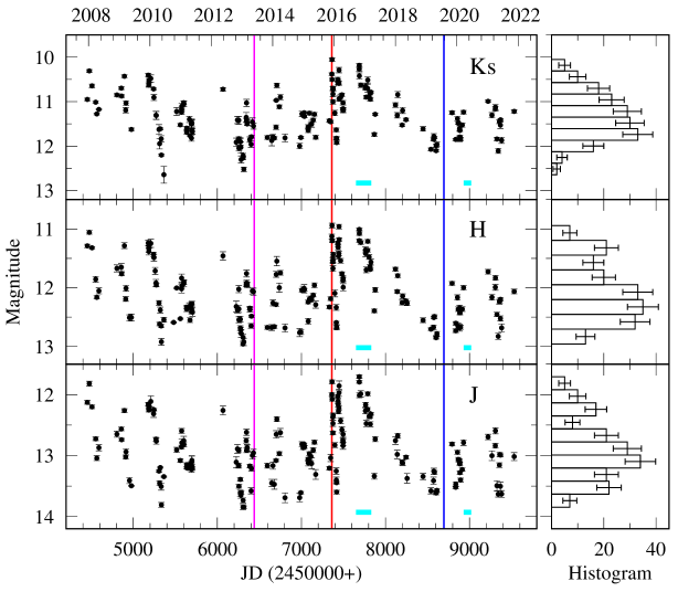
Figure 1: Multi-band NIR variability light curves of the blazar OJ 287 during 2007 December – 2021 November. From bottom to top, the left panels show J, H, and Ks calibrated magnitudes, respectively. The right panels show how many measurements fall into each equal bin, the widths of which are assigned through the Knuth method (Knuth, 2006) and differ slightly for each band. The magenta, red, and blue vertical lines, respectively, mark the first sighting of a rather sharp NIR-optical spectral break in end May 2013 and the flux peaks of the double-peaked outbursts of the $\sim 12$-yr QPO seen in end 2015 and mid 2019. The horizontal cyan lines mark the durations of the brightest X-ray activity phases as reported in the literature.

3 Results

In Figure 1 we present the J, H, and Ks band NIR photometric light curves (LCs) generated from our new observations taken during 2007 December – 2021 November. This is the most extensive and well-sampled long-term NIR photometric study of the blazar OJ 287. On visual inspection the J, H, and Ks band LCs all clearly show large amplitude flux variations. Several substantial flaring events in the photometric observations in all three bands are seen. In the following subsections, we discuss the NIR temporal and spectral variability properties of the blazar OJ 287 on LTV timescales.

3.1 LC Analysis Techniques

To calculate the amplitude of LTV variability and interband cross correlations in the NIR J, H, and Ks bands, the methods we used are briefly described below.

3.1.1 Amplitude of Variability

The percentage of the amplitude of the variability in magnitude (and color) on LTV timescales is described by the parameter, $A$, which can be defined using the following equation introduced by Heidt & Wagner (1996)

$$A=100\times\sqrt{{(A_{max}-A_{min}})^{2}-2\sigma^{2}}(\%)$$ (1)

Here $A_{max}$ and $A_{min}$ are the maximum and minimum values, respectively, in the calibrated magnitude or color of the LC of the blazar, and $\sigma$ is the mean measurement error.

3.1.2 Discrete Cross-correlation Function

We carried out the cross-correlation analysis between the NIR bands using the z-transformed Discrete Cross-correlation (zDCF; Alexander, 1997, 2013) method. It is broadly similar to the traditional DCF except that the correlation coefficient errors are estimated using the z-transform, given by

$$z=\frac{1}{2}ln\left(\frac{1+r}{1-r}\right),\zeta=\frac{1}{2}ln\left(\frac{1+\rho}{1-\rho}\right),r=tanh(z),$$

where $r$ and $\rm\rho$ represent the bin correlation coefficient and the unknown population correlation coefficient, respectively. The correlation coefficients are estimated by constructing all possible time lag data pairs ($x_{i}$, $y_{i}$) between the two light curves as

$$r=\frac{\sum_{i}^{n}(x_{i}-\overline{x})(y_{i}-\overline{y})}{\sigma_{x}\sigma_{y}},s_{x}^{2}=\frac{1}{n-1}\sum_{i}^{n}(x_{i}-\overline{x})^{2}.$$

In order to obtain the mean and variance of $z,\rho=r$ is assumed (Alexander, 2013). The reason for making the z-transformation is that the correlation coefficients are not normally distributed in the real space. This method is applicable to both uniformly and sparse, non-uniformly, sampled time series data. It employs Fisher’s z-transform and equal population binning to handle the bias arising due to sampling and skewness and fares better compared to the traditional approaches (Alexander, 1997, 2013). The errors were estimated using the Monte Carlo method by simulating 1000 pairs of light curves from the observed light curves by adding a Gaussian noise extracted from the measured error bars. The resulting cross-correlation results are shown in Figure 2. The peaks at zero lag signify that the multi-band NIR variations are simultaneous.

3.2 Long Term Variability

Our typical observational cadence of once a month, with a daily follow-up around the higher activity phases, allow us to explore long-term variations of OJ 287 in multi-band NIR flux, color, spectral index, and spectral energy distributions. We also discuss the detection of a large number of flaring events during the whole observing duration.

3.2.1 Flux Variability

Table 2: Results of LTV Flux Variations

Band	Duration	Variable	A(%)
J	2007-12-18 $-$ 2021-11-13	Var	213.9
H	2007-12-18 $-$ 2021-11-13	Var	201.4
Ks	2007-12-18 $-$ 2021-11-13	Var	259.1

Large amplitude significant flux variability from OJ 287 on LTV timescales is clearly visible from the three panels of Figure 1, where the J, H, and Ks band LCs are presented from bottom to top panels, respectively. We have calculated the variability amplitudes in the J, H, and Ks NIR photometric bands, and the results are reported in Table 2. We found the faintest level of the blazar in J, H, and Ks bands were 13.846 mag at JD 2456314.995185, 12.957 mag at JD 2456304.915382, and 12.645 mag at JD 2455363.648433, respectively. Similarly the observed brightest levels are 11.706 mag at JD 2457689.016863, 10.942 mag at JD 2457365.021296, and 10.053 mag at JD 2457365.027350, in the J, H, and Ks bands, respectively. In terms of fluxes, the amplitudes of variation given in Table 2 correspond to changes by a factor of roughly 7.2, 6.4, and 10.9 in the J, H, and Ks bands respectively. In the nearly 14 years long NIR observational duration, the large amplitude variations in the blazar LCs indicate that we have observed in the source in low, intermediate, high, and possibly even outburst, flux states. Historically, the brightest reported NIR magnitudes of OJ 287 were J = 10.73 mag, H = 9.94 mag, K = 8.81 mag and the faintest, J = 14.60 mag, H = 13.73 mag, K = 12.75 mag (Fan et al., 1998). If we compare them with our data presented here, it is clearly seen that we have observed the blazar right in between its historically brightest and faintest states.

Visually, it appears from Figure 1 that the J, H, Ks NIR bands follow the same variability pattern. To further examine the variability relations between these NIR bands, we performed DCF analyses using the zDCF method between these bands as shown in Figure 2. Strong correlations with zero lag are found in the different combination of all three NIR bands. These correlations strongly indicate that the emission in J, H, and Ks bands are cospatial and emitted from the same population of leptons.

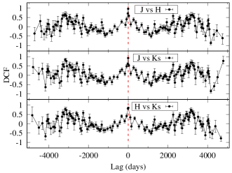
Figure 2: DCF plots using the zDCF method between NIR J, H, and Ks bands for the total duration of observations. The time lag and DCF values are given on the X-axis and Y-axis, respectively.

3.2.2 Color Variability

Table 3: Color Variation with Respect to Time on LTV

Color	$\rm m_{2}(\times 10^{-6})$	$\rm c_{2}$	$\rm r_{2}$	$\rm p_{2}$
Indices
J – H	$-$11.3$\rm\pm$5.9	28$\rm\pm$14	0.017	0.06
J – Ks	$-$11.3$\rm\pm$8.0	29$\rm\pm$19	0.006	0.16
H – Ks	0.31$\rm\pm$7.61	0$\rm\pm$18	$-$0.006	0.97

Note: m₂ = slope and c₂ = intercept of color against H mag; r₂ = coefficient of determination ($\rm R^{2}$); p₂ (0.05) = null hypothesis rejection probability.

Table 4: Color Variation with Respect to H-band magnitude on LTV

Color	$\rm m_{2}$	$\rm c_{2}$	$\rm r_{2}$	$\rm p_{2}$
Indices
J – H	-0.026 $\rm\pm$0.015	1.14$\rm\pm$0.18	0.013	0.08
J – Ks	-0.018 $\rm\pm$0.022	1.80$\rm\pm$0.26	-0.002	0.41
H – Ks	0.028 $\rm\pm$0.020	0.41$\rm\pm$0.24	0.007	0.16

Note: m₂ = slope and c₂ = intercept of color against H mag; r₂ = coefficient of determination ($\rm R^{2}$); p₂ (0.05) = null hypothesis rejection probability.

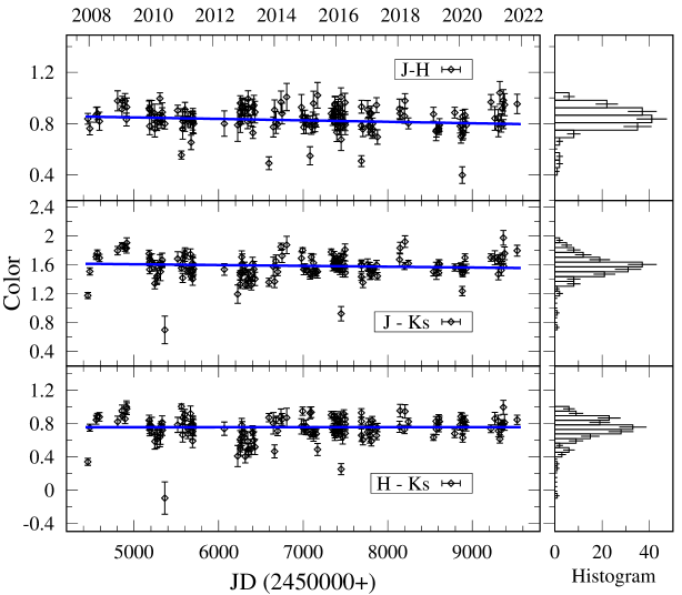
Figure 3: As in Fig. 1 for the NIR color variability for the entire duration of these observations of OJ 287. The panels on the right show the spectral index histogram.

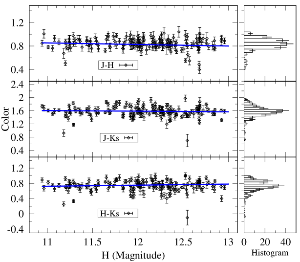
Figure 4: As in Fig. 3 for NIR color–magnitude plots for OJ 287.

For the total duration of our observations of OJ 287, NIR color variations with respect to time (color vs. time) and with respect to H-band magnitude (color vs. magnitude) are displayed in Figures 3 and 4, respectively. On visual inspection both figures show weak evidence of color variations, but there are no consistent systematic trends in the color variations with respect to time or H-band magnitude. To further examine the color variation, we did straight line fits to the color versus time, and color versus H-mag, plots in Figure 3 and Figure 4, respectively. The straight line fit parameters values e.g., the slopes, $m$, the intercepts, $c$, the linear Pearson correlation coefficients, $r$, and the corresponding null hypothesis rejection probability, $p$, for color versus time and color versus H-band magnitude are given in Tables 3 and 4, respectively.

3.2.3 Spectral Index Variations and SEDs

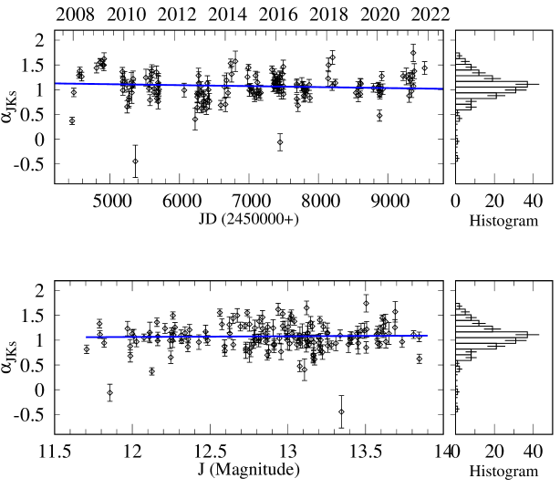
Figure 5: NIR spectral index variation with time and J-band magnitude covering the entire observation period of OJ 287. The panels on the right show the spectral index histogram.

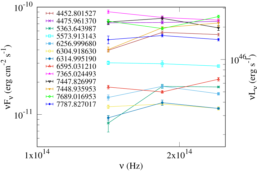
Figure 6: Plot showing a glimpse of diverse NIR spectral phases of OJ 287. The accompanying video shows the NIR SED evolution with time. The video duration is 17 seconds.

In these magnitude measurements the color variations encode spectral information across the NIR. Making the assumption of a power-law spectrum across these bands we find

$$\alpha_{JKs}=\frac{(F_{J}/F_{Ks})}{(\nu_{J}/\nu_{Ks})},$$ (2)

where $F_{J}$ and $F_{Ks}$ are fluxes calculated using the 2MASS zero values from Cohen et al. (2003) with respective central frequencies of these bands $\rm\nu_{J}$ and $\rm\nu_{Ks}$. The reddening corrections for the J, H, and Ks bands are respectively 0.02149, 0.01332, and 0.00874 mag (Cardelli et al., 1989, using $\rm R_{V}$ = 3.1 and $\rm E(B-V)=0.0241$).

Figure 5 shows these spectral changes with time as well as with source flux states in the J band. Neither of these show any systematic trend over the long-term, as highlighted by the flat linear regression fits to them presented in Table 5. However, there are significant fluctuations around the mean, indicating spectral variations over short-time scales as reflected in the histograms shown in the right panels of figure 5. The histograms are skewed towards larger values of $\alpha_{Ks}$ indicating a tendency toward spectral steepening; however, there are a few instances showing spectral hardening.

The fluxes vary over almost an order of magnitude. The NIR SEDs, showing the diverse spectral facets exhibited by the source in between the minimum and maximum NIR flux states are shown in Figure 6. The accompanying video presents a complete view of NIR SEDs with time. In general, the SEDs are flat or declining, with most being consistent with a power-law spectrum (within a 10% error). Occasionally, there are hints of smooth departures at the low energy end as well of hardening.

Table 5: Spectral Index Variation with Respect to JD and J-band Magnitude for the Entire Period of the Observations of OJ 287

Parameter	$\rm m_{2}$	$\rm c_{2}$	$\rm r_{2}$	$\rm p_{2}$
$\alpha_{JKs}$ vs JD	(-1.9$\rm\pm$1.4)$\times 10^{-5}$	48$\rm\pm$33	0.006	0.16
$\alpha_{JKs}$ vs J (mag)	0.014$\rm\pm$0.038	0.90$\rm\pm$0.49	-0.006	0.72

Note: m₂ = slope and c₂ = intercept of $\alpha_{JKs}$ against JD or J;
r₂ = coefficient of determination ($\rm R^{2}$); p₂ (0.05) = null hypothesis rejection probability.

3.2.4 Flaring and outbursts

During the nearly 14 years (2007 December – 2021 November) of our intense multi-band NIR observations of OJ 287 the source exhibited several well defined large amplitude flares seen in all these J, H, and Ks bands, plotted in Figure 1 from bottom to top panels, respectively. We performed NIR inter-band cross correlation analysis using ZDCF and plotted this in Figure 2. From Figure 2, we found that J, H, and Ks bands fluxes are strongly correlated without any lag, so any observed flare in any of these J, H, and Ks bands are certainly observed quasi-simultaneously in the other two bands.

4 Discussion

The current study presents the most up-to-date and extensive NIR spectral and temporal behavior of OJ 287 for the lengthy period of 2007 December – 2021 November. Despite annual and inhomogeneous sampling related gaps, the NIR fluxes are well-sampled from high to low states, with denser sampling ($\sim 1-2$ days interval) around and after the high states. This is true for almost every period of activity, as is clear from Fig. 1.

The source has undergone strong and quite frequent outbursts in NIR bands that are simultaneous within the observational cadence (Fig. 2). The respective magnitude histograms are skewed, with more gradual falloffs on the brighter side but steeper declines on the fainter side. This skewness, however, is most likely from a sampling bias favoring brighter state follow-up and could also have a minor effect from the change of base level brightness, as discussed in the next paragraph. The time series reveal strong NIR flux variations with amplitudes almost similar to the optical bands of the same duration (Bonning et al., 2012; Sandrinelli et al., 2014; Gupta et al., 2017, 2019). There is almost an order of magnitude difference between the extremes (see Fig. 6). Over long-term timescales, there is no systematic spectral evolution or trend either with time (Fig. 3) or flux state of the source (Fig. 4). However, during the bright phases, the flux changes are often associated with significant color variations over the short-term, as highlighted by the fluctuations around the mean in the color (Figs. 4 & 3) and spectral evolution plots (Figs. 5 & 6). The color/spectral evolution with time and source brightness too are skewed, with a tendency for larger J-H color/spectral variations indicating steepening of the spectrum with source brightness over short-term flaring episodes. Contrary to this general trend, a few instances show appreciable hardening (Fig. 5).

The behaviors reported here are largely in line with those reported previously for OJ 287 at NIR bands (e.g. Zhang & Xie, 1996; Fan et al., 1998; Bonning et al., 2012; Sandrinelli et al., 2014) and most of the seemingly contrary behavior can largely be attributed to sampling bias of the previous studies and the change in base-level brightness. For example, the typical brightness in J, H, and Ks bands are 12.9, 12.0, and 11.3 with a typical standard variation of $\sim 0.5$ mag in each and a $\rm 2.0-2.5$ mag difference between the extremes. These brightness levels are in between the reported historical NIR brightness levels (1971 onwards) and so are the differences of the extremes ($\sim 3.5$ mag; Fan et al., 1998). However, since both the NIR and optical emissions are synchrotron and lie on the extension of the same power-law spectral component (at and after the low-hump SED peak), the century long optical light curve can be used to examine any systematic/trends. This light curve indicates a systematic decline of base level brightness around 1 magnitude between 1971 and 2000 which reverses from 2000 onwards, with jet related short-term and large amplitude flares superposed on it (see Fig. 1 of Dey et al., 2018). Thus, the variations and differences between the extremes are similar to those we see once the base brightness is taken into account. Similarly, the general tendency of larger J-K/J-Ks color (indicating steepening of spectra) reported in earlier studies involving NIR and optical data (Zhang & Xie, 1996, and references therein) is consistent with our results during flaring. The long-term systematic trend reported in Zhang & Xie (1996) is likely a sampling bias as is clear from the light curve which shows a systematic decrease in flux before and after the most brightened event.

The current NIR observations are also the first NIR data taken during the brightest X-ray phases of this source that were seen in the years 2016–2017 and 2020 (Komossa et al., 2020) — a result of a new high synchrotron peaked BL Lac (HBL) type of broadband emission component (Kushwaha et al., 2018b, 2021; Singh et al., 2022). Both these bright X-ray phases came after the claimed double-peaked outbursts: the 2015 (Valtonen et al., 2016) and 2019 (Laine et al., 2020) flares of the $\rm\sim 12$-yr optical QPOs. As the NIR variation amplitude is similar to that seen in the optical (Gupta et al., 2017, 2019) we can conclude that these overall variations are due to a jet emission component rather than the new, thermal-like, emission component seen during the 2013 – 2016 at the interface of NIR-optical bands (Kushwaha et al., 2018a). This is also consistent with the brightest reported X-ray phases of the source being an HBL-like emission component.

Apart from these general trends, OJ 287 on short-terms at different activity phases has shown very diverse and contrary behaviors. For example, none of the low state SEDs presented here indicate any new emission component, but at most a spectral hardening; however, on a few occasions, NIR-optical data show otherwise (Sandrinelli et al., 2014). A hysterisis has also been reported involving redder-when-brighter and bluer-when-brighter trends as well as color changes at fixed magnitude (Bonning et al., 2012). The current observations also make it clear that the extreme and odd variability seen only in the K-band magnitude from the SMARTS database that persisted for almost an observing cycle (JD: $\rm\sim$ 2455500 – 2455710), as reported in Kushwaha (2021), is most likely artificial. In short, although blazars are known for dynamic flux variability, they rarely show significant spectral departures in the broadband SEDs. OJ 287, on the other hand, is quite unique with sepctral changes persisting for much longer time (e.g. Brien & VERITAS Collaboration, 2017; Kushwaha et al., 2018a, b, 2021; Prince et al., 2021; Singh et al., 2022) and thus, a potential source for fresh inputs not only on relativistic jets above what is generally known about blazars but also on aspects related to accretion as well (e.g. Kushwaha, 2020, 2021).

5 Summary

We have presented the most up-to date and extensive NIR observations of OJ 287 between 2007 to 2021. A summary of our results and inferences are as follows:

1. OJ 287 shows strong NIR variations with a brightness changes of $\rm\gtrsim 2$ mag between the extremes. These variations are similar to those reported previously once the base level brightness is taken out, as indicated by the optical light curve exceeding a century in length.

2. The NIR variations are simultaneous within the limits of observational cadence.

3. There is no general tendency for color variations over this extended period either with the flux or with time. However, over short-times (bright phases) the NIR spectrum steepens with brightness and vice-versa. This tendency is similar to those reported in the literature in the optical and NIR bands.

4. A few of these observations show hardening of the NIR spectrum, possibly indicating a shift in the synchrotron SED peak, though they are not clearly significant.

5. The current NIR data includes the first data taken in these bands for bright X-ray phases. As those variabilities are similar to those in the optical they should arise from a broadband emission component.

References

- Alexander (1997) Alexander, T. 1997, Astronomical Time Series, 218, 163. doi:10.1007/978-94-015-8941-3_14
- Alexander (2013) Alexander, T. 2013, arXiv:1302.1508
- Astropy Collaboration et al. (2013) Astropy Collaboration, Robitaille, T. P., Tollerud, E. J., et al. 2013, A&A, 558, A33. doi:10.1051/0004-6361/201322068
- Astropy Collaboration et al. (2018) Astropy Collaboration, Price-Whelan, A. M., Sipőcz, B. M., et al. 2018, AJ, 156, 123. doi:10.3847/1538-3881/aabc4f
- Baker et al. (2019a) Baker, J., Bellovary, J., Bender, P. L., et al. 2019a, arXiv:1907.06482
- Baker et al. (2019b) Baker, J., Haiman, Z., Rossi, E. M., et al. 2019b, BAAS, 51, 123
- Bhatta et al. (2016) Bhatta, G., Zola, S., Stawarz, Ł., et al. 2016, ApJ, 832, 47. doi:10.3847/0004-637X/832/1/47
- Bonning et al. (2012) Bonning, E., Urry, C. M., Bailyn, C., et al. 2012, ApJ, 756, 13. doi:10.1088/0004-637X/756/1/13
- Brien & VERITAS Collaboration (2017) Brien, S. O. & VERITAS Collaboration 2017, 35th International Cosmic Ray Conference (ICRC2017), 301, 650
- Britzen et al. (2018) Britzen, S., Fendt, C., Witzel, G., et al. 2018, MNRAS, 478, 3199. doi:10.1093/mnras/sty1026
- Burke-Spolaor et al. (2019) Burke-Spolaor, S., Taylor, S. R., Charisi, M., et al. 2019, A&A Rev., 27, 5. doi:10.1007/s00159-019-0115-7
- Butuzova & Pushkarev (2020) Butuzova, M. S. & Pushkarev, A. B. 2020, Universe, 6, 191. doi:10.3390/universe6110191
- Cardelli et al. (1989) Cardelli, J. A., Clayton, G. C., & Mathis, J. S. 1989, ApJ, 345, 245. doi:10.1086/167900
- Carrasco et al. (1985) Carrasco, L., Dultzin-Hacyan, D., & Cruz-Gonzalez, I. 1985, Nature, 314, 146. doi:10.1038/314146a0
- Carrasco et al. (2017) Carrasco, L., Hernández Utrera, O., Vázquez, S., et al. 2017, Rev. Mexicana Astron. Astrofis., 53, 497
- Chen & Zhang (2018) Chen, J.-W. & Zhang, Y. 2018, MNRAS, 481, 2249. doi:10.1093/mnras/sty2268
- Cohen et al. (2003) Cohen, M., Wheaton, W. A., & Megeath, S. T. 2003, AJ, 126, 1090. doi:10.1086/376474
- Dey et al. (2018) Dey, L., Valtonen, M. J., Gopakumar, A., et al. 2018, ApJ, 866, 11
- Epstein et al. (1972) Epstein, E. E., Fogarty, W. G., Hackney, K. R., et al. 1972, ApJ, 178, L51. doi:10.1086/181083
- Fan et al. (1998) Fan, J. H., Adam, G., Xie, G. Z., et al. 1998, A&AS, 133, 163. doi:10.1051/aas:1998314
- Fossati et al. (1998) Fossati, G., Maraschi, L., Celotti, A., et al. 1998, MNRAS, 299, 433. doi:10.1046/j.1365-8711.1998.01828.x
- Gear et al. (1986) Gear, W. K., Robson, E. I., & Brown, L. M. J. 1986, Nature, 324, 546. doi:10.1038/324546a0
- Gupta et al. (2004) Gupta, A. C., Banerjee, D. P. K., Ashok, N. M., et al. 2004, A&A, 422, 505. doi:10.1051/0004-6361:20040306
- Gupta et al. (2017) Gupta, A. C., Agarwal, A., Mishra, A., et al. 2017, MNRAS, 465, 4423. doi:10.1093/mnras/stw3045
- Gupta et al. (2019) Gupta, A. C., Gaur, H., Wiita, P. J., et al. 2019, AJ, 157, 95. doi:10.3847/1538-3881/aafe7d
- Heidt & Wagner (1996) Heidt, J. & Wagner, S. J. 1996, A&A, 305, 42
- Holmes et al. (1984a) Holmes, P. A., Brand, P. W. J. L., Impey, C. D., et al. 1984a, MNRAS, 210, 961. doi:10.1093/mnras/210.4.961
- Holmes et al. (1984b) Holmes, P. A., Brand, P. W. J. L., Impey, C. D., et al. 1984b, MNRAS, 211, 497. doi:10.1093/mnras/211.3.497
- Kidger et al. (1995) Kidger, M. R., Gonzalez-Perez, J. N., de Diego, J. A., et al. 1995, A&AS, 113, 431
- Knuth (2006) Knuth, K. H. 2006, arXiv:physics/0605197
- Komossa et al. (2017) Komossa, S., Grupe, D., Schartel, N., et al. 2017, New Frontiers in Black Hole Astrophysics, 324, 168. doi:10.1017/S1743921317001648
- Komossa et al. (2020) Komossa S., Grupe D., Parker M. L., Valtonen M. J., Gómez J. L., Gopakumar A., Dey L., 2020, MNRAS, 498, L35
- Kushwaha (2020) Kushwaha, P. 2020, Galaxies, 8, 15. doi:10.3390/galaxies8010015
- Kushwaha (2021) Kushwaha, P. 2021, arXiv:2110.10851
- Kushwaha et al. (2022) Kushwaha, P., Gupta, A. C., Wiita, P. J., et al. 2022, in preparation
- Kushwaha et al. (2018a) Kushwaha, P., Gupta, A. C., Wiita, P. J., et al. 2018a, MNRAS, 473, 1145
- Kushwaha et al. (2018b) Kushwaha, P., Gupta, A. C., Wiita, P. J., et al. 2018b, MNRAS, 479, 1672
- Kushwaha et al. (2021) Kushwaha, P., Pal, M., Kalita, N., et al. 2021, ApJ, 921, 18. doi:10.3847/1538-4357/ac19b8
- Kushwaha et al. (2020) Kushwaha, P., Sarkar, A., Gupta, A. C., et al. 2020, MNRAS, 499, 653. doi:10.1093/mnras/staa2899
- Laine et al. (2020) Laine, S., Dey, L., Valtonen, M., et al. 2020, ApJ, 894, L1. doi:10.3847/2041-8213/ab79a4
- Lehto & Valtonen (1996) Lehto, H. J., & Valtonen, M. J. 1996, ApJ, 460, 207
- Litchfield et al. (1994) Litchfield, S. J., Robson, E. I., & Stevens, J. A. 1994, MNRAS, 270, 341. doi:10.1093/mnras/270.2.341
- Marscher (1983) Marscher, A. P. 1983, ApJ, 264, 296. doi:10.1086/160597
- Miller et al. (1989) Miller, H. R., Carini, M. T., & Goodrich, B. D. 1989, Nature, 337, 627. doi:10.1038/337627a0
- Mücke et al. (2003) Mücke, A., Protheroe, R. J., Engel, R., et al. 2003, Astroparticle Physics, 18, 593. doi:10.1016/S0927-6505(02)00185-8
- O’Brien (2017) O’Brien, S. 2017, arXiv:1708.02160
- Pal et al. (2020) Pal, M., Kushwaha, P., Dewangan, G. C., et al. 2020, ApJ, 890, 47. doi:10.3847/1538-4357/ab65ee
- Prince et al. (2021) Prince, R., Agarwal, A., Gupta, N., et al. 2021, A&A, 654, A38. doi:10.1051/0004-6361/202140708
- Pursimo et al. (2000) Pursimo, T., Takalo, L. O., Sillanpää, A., et al. 2000, A&AS, 146, 141. doi:10.1051/aas:2000264
- Romero et al. (2017) Romero, G. E., Boettcher, M., Markoff, S., et al. 2017, Space Sci. Rev., 207, 5. doi:10.1007/s11214-016-0328-2
- Sandrinelli et al. (2014) Sandrinelli, A., Covino, S., & Treves, A. 2014, A&A, 562, A79. doi:10.1051/0004-6361/201321558
- Seabold et al. (2010) Seabold, Skipper, and Josef Perktold. “statsmodels: Econometric and statistical modeling with python.” Proceedings of the 9th Python in Science Conference. 2010
- Sillanpää et al. (1988) Sillanpää, A., Haarala, S., Valtonen, M. J., et al. 1988, ApJ, 325, 628. doi:10.1086/166033
- Sillanpää et al. (1996a) Sillanpää, A., Takalo, L. O., Pursimo, T., et al. 1996a, A&A, 305, L17
- Sillanpää et al. (1996b) Sillanpää, A., Takalo, L. O., Pursimo, T., et al. 1996b, A&A, 315, L13
- Singh et al. (2022) Singh, K. P., Kushwaha, P., Sinha, A., et al. 2022, MNRAS, 509, 2696. doi:10.1093/mnras/stab3161
- Sitko & Junkkarinen (1985) Sitko, M. L. & Junkkarinen, V. T. 1985, PASP, 97, 1158. doi:10.1086/131679
- Stetson (1987) Stetson, P. B. 1987, PASP, 99, 191. doi:10.1086/131977
- Takalo et al. (1992) Takalo, L. O., Kidger, M. R., de Diego, J. A., et al. 1992, AJ, 104, 40. doi:10.1086/116219
- Tody (1986) Tody, D. 1986, Proc. SPIE, 627, 733. doi:10.1117/12.968154
- Urry & Padovani (1995) Urry, C. M. & Padovani, P. 1995, PASP, 107, 803. doi:10.1086/133630
- Valtaoja et al. (1985) Valtaoja, E., Lehto, H., Teerikorpi, P., et al. 1985, Nature, 314, 148. doi:10.1038/314148a0
- Valtonen et al. (2009) Valtonen, M. J., Nilsson, K., Villforth, C., et al. 2009, ApJ, 698, 781. doi:10.1088/0004-637X/698/1/781
- Valtonen et al. (2016) Valtonen, M. J., Zola, S., Ciprini, S., et al. 2016, ApJ, 819, L37. doi:10.3847/2041-8205/819/2/L37
- Visvanathan & Elliot (1973) Visvanathan, N. & Elliot, J. L. 1973, ApJ, 179, 721. doi:10.1086/151911
- Wagner & Witzel (1995) Wagner, S. J. & Witzel, A. 1995, ARA&A, 33, 163. doi:10.1146/annurev.aa.33.090195.001115
- Wolstencroft et al. (1982) Wolstencroft, R. D., Gilmore, G., & Williams, P. M. 1982, MNRAS, 201, 479. doi:10.1093/mnras/201.2.479
- Woo & Urry (2002) Woo, J.-H., & Urry, C. M. 2002, ApJ, 579, 530. doi:10.1086/342878
- Zhang & Xie (1996) Zhang, Y.-H. & Xie, G.-Z. 1996, A&AS, 119, 199