Rarefaction effects in head-on collision of two identical droplets

Abstract

The head-on collision of two identical droplets is investigated based on the BGK-Boltzmann equation. Gauss-Hermite quadratures with different degree of precision are used to solve the kinetic equation, so that the continuum (solution truncated at the Navier-Stokes order) and non-continuum (rarefied gas dynamics) solutions can be compared. When the kinetic equation is solved with adequate accuracy, prominent variations of the vertical velocity (the collision is in the horizontal direction), the viscous stress components, and droplet morphology are observed during the formation of liquid bridge, which demonstrates the importance of the rarefaction effects and the failure of the Navier-Stokes equation. The rarefaction effects change the topology of streamlines near the droplet surface, suppress the high-magnitude vorticity concentration inside the interdroplet region, and promote the vorticity diffusion around outer droplet surface. Two physical mechanisms responsible for the local energy conversion between the free and kinetic energies are identified, namely, the total pressure-dilatation coupling effect and the interaction between the density gradient and strain rate tensor. An energy conversion analysis is performed to show that the rarefaction effects can enhance the conversion from free energy to kinetic energy and facilitate the discharge of interdroplet gas film along the vertical direction, thereby boosting droplet coalescence.

1 Introduction

Studying the droplet collision dynamics is of fundamental importance in understanding a variety of natural phenomena and engineering problems, such as atmospheric raindrop formation, ink-jet printing, dense spray system, and so on. Undoubtedly, complex interactions among a large number of droplets impose great difficulties in quantitative measurements and analysis. Therefore, the binary droplet collision problem is usually used as a canonical case for studying the physics of droplet collisions.

The droplet collision is affected by many dimensionless parameters. Previous studies are devoted to identifying and interpreting the outcomes of binary collision in the continuum regime where the Navier-Stokes equation is valid, such as the coalescence, separation, bouncing, and shattering. Different collision outcomes are well summarized in a $We$-$B$ regime diagram ($We$ is the Weber number and $B$ is the impact parameter), where some phenomenological criteria are also proposed to predict their transition boundaries for both the water and hydrocarbon droplets (Ashgriz & Poo, 1990; Jiang et al., 1992; Qian & Law, 1997; Orme, 1997; Pan et al., 2008, 2009). In this paper, we are interested in the role of gas cushion in the droplet collision, since it has been observed that increasing (decreasing) the ambient gas pressure promotes droplet bouncing (coalescence) (Jiang et al., 1992; Qian & Law, 1997; Zhang et al., 2016).

When the thickness of gas film between the colliding droplets is small, the rarefied (or non-continuum) gas dynamics beyond the description of Navier-Stokes equations should be considered. However, they are relatively less investigated in problems of binary droplet collision, probably due to the complexity in the Boltzmann-type kinetic equation. Therefore, several simplified methods are used to account for the rarefaction effects. Zhang & Lister (1999) first studied the van der Waals rupture of a thin film on a solid substrate using the disjoint pressure model which was later adopted by several researchers to explore the binary droplet collision dynamics (Jiang & James, 2007; Yoon et al., 2007). Starting from the linearised Boltzmann equation, Zhang & Law (2011) derived a modified lubrication force expression to account for the rarefaction effects inside the interdroplet gas film. It was found that the lubrication pressure was only modified by a correction factor for the shear viscosity of the gas. Li (2016) made two corrections to the axisymmetric Navier-Stokes equations to account for the rarefied nature of the interdroplet gas film. On one hand, the disjoint pressure model of Zhang & Lister (1999) was used to incorporate the intermolecular van de Waals forces in a sharp-interface description. On the other hand, the modified shear viscosity model of Zhang & Law (2011) was adopted to describe the rarefaction effects. It is reported that the disjoint pressure model provides a leading-order approximation for relatively flat interfaces, but fails to capture the flow physics involved during the final stage of gas film rupture and therefore is not robust in predicting droplet coalescence (Yoon et al., 2007; Chen & Yang, 2020). For low-Reynolds-number collision of two rigid spheres moving in an ideal isothermal gas, it is found that either the non-continuum or compressible effect allows the particles to contact, while a continuum incompressible lubrication would prevent particle contact (Gopinath et al., 1997). This indicates that both the compressible and non-continuum nature of the gas should be included in an accurate macroscopic description of the collision process. There also exist some studies relevant to the rarefaction effects in the gas film, which includes a high-speed liquid splash on a dry solid surface (Mandre & Brenner, 2012), air entrainment in dynamic wetting (Sprittles, 2015, 2017), and the creation of anti-bubbles from air films (Beilharz et al., 2015).

The aforementioned studies indicate that when the characteristic film thickness is comparable to the mean free path of gas molecules, the no-slip boundary condition breaks down and hence the rarefaction effects should be considered in the physical modelling. The slip effect decreases the lubrication resistance in the gap flow, which facilitates the drainage of the gas and the rupture of the film, therefore boosting the liquid-solid or liquid-liquid contact. In addition, by reducing the ambient gas pressure, the mean free path of the gas increases, which implies the enhancement of the rarefaction effect within the gas film.

As the characteristic Knudsen number (i.e., the ratio of the mean free path to the characteristic length scale) increases, the Navier-Stokes equation is no longer adequate to capture the fundamental physics: not only the slip velocity condition arises, but also the constitutive relation breaks down. Although the modified macroscopic equations can deal with certain problems, there is no self-consistent way macroscopically to include higher-order non-continuum effects in an a priori manner (Shan et al., 2006). On the other hand, although the 13-moment and 26-moment equations can go beyond the Navier-Stokes equations and capture the flow physics up to a certain Knudsen-number order (Rana et al., 2021; Struchtrup & Frezzotti, 2022), their derivation and numerical simulation are rather complicated, and their validity region is limited. For such scenarios, the Boltzmann-type kinetic equation is more fundamental to include the higher-order non-continuum effects beyond the Navier-Stokes level, which provides an unified kinetic description for different flow regimes. To the authors’ knowledge, rarefaction effects in head-on collision of two droplets are not yet investigated by solving the kinetic equation, which becomes the main topic of the present study.

The rest of this paper is organized as follows. In Section 2, we provide a brief introduction to the free-energy-based multiphase flow model. In Section 3, we briefly review the progresses on kinetic modelling of single-component liquid-vapour flows and then introduce the present thermodynamically consistent mesoscopic model. In addition, we describe the details of the numerical method and the construction of Gauss-Hermite quadratures. Then, numerical simulations are performed in Section 4, where we discuss the rarefaction effects on macroscopic quantities, droplet morphology, streamline topology and energy conversion. Finally, conclusions are drawn in Section 5.

2 Free-energy-based multiphase flow model

The quasi-local thermodynamics of a two-phase flow system at equilibrium can be described by the second-gradient theory through the density and its gradient (Cahn & Hilliard, 1958; Rowlinson & Widom, 1982; Anderson et al., 1998; Yue et al., 2004). The corresponding free energy functional is given by

$$\mathcal{F}(\rho,\bm{\nabla}\rho)=\int_{V}\left(\psi(\rho)+\frac{1}{2}\kappa\lVert\bm{\nabla}\rho\rVert^{2}\right)dV,$$ (1)

where $\rho$ is the density, $\kappa$ is the interfacial free energy coefficient associated with the surface tension coefficient $\sigma_{s}$, and $V$ is the integral domain occupied by the fluids. The first term represents the bulk free energy density and the second term is the interfacial free energy density caused by the non-local molecular interactions.

In the present paper, the double-well formulation of the bulk free energy density is employed (Jacqmin, 1999; Jamet et al., 2001):

$$\psi(\rho)=\beta(\rho-\rho_{l})^{2}(\rho-\rho_{g})^{2},$$ (2)

where $\rho_{l}$ and $\rho_{g}$ represent the densities of liquid and vapour phases at saturation, respectively, and $\beta$ is a positive constant coefficient. Equation (2) works perfectly in the vicinity of the critical point of the equation of state while may cease to be valid away from the critical point, namely, at a large density ratio or an equivalently low temperature (Lee & Fischer, 2006; Yue et al., 2004). Therefore, the present paper only considers the near-critical fluids with small density ratio.

The first-order variation of the free energy functional with respect to the density defines the chemical potential $\mu_{\rho}$ as follows:

$$\mu_{\rho}\equiv\frac{\delta\mathcal{F}}{\delta\rho}=\frac{\partial\psi}{\partial\rho}-\kappa\nabla^{2}\rho.$$ (3)

Moreover, for a given $\psi$, the thermodynamic pressure $p_{0}$ (i.e., the equation of state) is determined by

$$p_{0}=\rho\frac{\partial\psi}{\partial\rho}-\psi.$$ (4)

Using (2), the bulk chemical potential is evaluated as $\mu_{0}\equiv{\partial\psi}/{\partial\rho}=4\beta(\rho-\rho_{l})(\rho-\rho_{g})[\rho-(\rho_{l}+\rho_{g})/2]$ and the corresponding thermodynamic pressure is $p_{0}=\beta(\rho-\rho_{l})(\rho-\rho_{g})[3\rho^{2}-\rho_{l}\rho_{g}-\rho(\rho_{l}+\rho_{g})]$.

For a flat surface at equilibrium, the density profile across the interface can be obtained by solving the energy-minimized equation $\mu_{\rho}=0$, which results in

$$\rho(\zeta)=\frac{\rho_{l}+\rho_{g}}{2}+\frac{\rho_{l}-\rho_{g}}{2}\tanh\left(\frac{2\zeta}{W}\right),$$ (5)

where $\zeta$ is the surface normal coordinate measured from the point satisfying $\rho=(\rho_{l}+\rho_{g})/2$ and $W=(\rho_{l}-\rho_{g})^{-1}\sqrt{8\kappa/\beta}$ is a length parameter with the same order of magnitude as the interfacial thickness. The surface tension coefficient $\sigma_{s}$ is equal to the integral of free energy density through the interface per unit area (Jacqmin, 1999, 2000). From (5), it is explicitly expressed as

$$\sigma_{s}=\kappa\int_{-\infty}^{+\infty}\left(\frac{d\rho}{d\zeta}\right)^{2}d\zeta=\frac{1}{6}(\rho_{l}-\rho_{g})^{3}\sqrt{2\kappa\beta}.$$ (6)

Conversely, a simple calculation will give

$$\beta=\frac{12\sigma_{s}}{W(\rho_{l}-\rho_{g})^{4}},\quad\kappa=\frac{3\sigma_{s}W}{2(\rho_{l}-\rho_{g})^{2}},$$ (7)

which can be used to determine $\beta$ and $\kappa$ when $\sigma_{s}$, $W$ and saturation densities are given.

3 Mesoscopic model and numerical method

A brief summary of the progresses on kinetic modelling of single-component liquid-vapour flows is given in order to provide a research background for the present study. An approximate kinetic consideration leads to the Enskog-Vlasov equation, which can be viewed as an extension of the Boltzmann equation for dilute gases to single-component multiphase flows with interfacial dynamics. The Enskog-Vlasov equation handles the short-range repulsive interaction among molecules using the Enskog kinetic theory for hard-sphere dense fluids (Chapman & Cowling, 1970) and incorporates the long-range attractive interaction by the mean-field approximation (Vlasov, 1968). Together with its modified versions, they have been applied to investigate evaporation of a liquid slab into near vacuum (Frezzotti et al., 2005), net evaporation and condensation (Kon et al., 2014), fluid-solid and vapour-solid interactions (Gibelli et al., 2015), thermodynamics of noble gases (Benilov & Benilov, 2018, 2019), evaporation of multicomponent substances into vapour and vacuum (Kobayashi et al., 2017; Frezzotti et al., 2018; Busuioc et al., 2020). Similar kinetic models were also proposed to deal with surface-confined strongly inhomogeneous flows in nanoscale shale gas transport (Guo et al., 2005).

However, the collision and mean-field force terms of the original Enskog-Vlasov equation are too complex for practical applications. In order to save the computational costs, simplifying the Enskog collision operator was also performed by applying the first-order Taylor-series expansion in terms of the molecular diameter (Chapman & Cowling, 1970; Kremer & Rosa, 1988), the Bhatnagar-Gross-Krook (BGK) or Shakhov approximation (Luo, 2000; He & Doolen, 2002; Wang et al., 2020; Huang et al., 2021), as well as the Fokker-Planck approximation (Sadr & Gorji, 2017). In addition, a simplified mean-field force expression was also derived using the Taylor-series expansion (namely, the smooth density approximation) (He & Doolen, 2002).

Although the (simplified) Enskog-Vlasov equation has inherent kinetic advantages for accurate interfacial description, the macroscopic or simplified mesoscopic models (methods) are preferred by taking into account both the model complexity and computational costs. So far, the continuum methods are extensively used. Numerous computational fluid dynamics (CFD) methods have been proposed to solve the Navier-Stokes equation, which include the front-tracking method, the level set method, and the volume-of-fluid method (Scardovelli & Zaleski, 1999; Sethian & Smereka, 2003). The front-tracking method is usually not able to simulate interface coalescence and break-up phenomena. For the level set and volume-of-fluid methods, the interface reconstruction or reinitialization may introduce some non-physical numerical artifacts. Over the past few decades, the lattice Boltzmann method (LBM) has been developed as an efficient mesoscopic CFD method, which allows a direct mesoscopic modelling of many complex physical problems covering both the single-phase and multiphase flows (Chen & Doolen, 1998; Shan et al., 2006). Prevalent multiphase LBM models include the colour-gradient model (Gunstensen et al., 1991), Shan-Chen model (Shan & Chen, 1993, 1994; Li et al., 2020), free-energy model (Swift et al., 1995, 1996), and phase field model (He et al., 1999; Yue et al., 2004; Zhang et al., 2018), which have been successfully applied to simulate a vast majority of multiphase flows at the continuum regime, with the superior advantage that the interfacial fluid dynamics can be automatically captured by incorporating a non-ideal equation of state and the intermolecular force during the particle collision and streaming processes.

The aforementioned LBM models with on-lattice discrete particle velocity sets are originally designed for the continuum flows where the rarefaction effects are not considered. As the Knudsen number increases, higher-order non-continuum effects become more and more significant. Recently, part of the rarefaction effects are considered by the 13- and 26-moment equations (Struchtrup & Frezzotti, 2019, 2022), which are derived from the Enskog-Vlasov equation. However, the derivation and numerical computation are rather complicated. In this paper, we aim to solve the kinetic equation for multiphase flows by a multiscale mesoscopic method which, through the proper discretization of molecular velocity space, can provide solutions either equivalent to the 13- and 26-moment equations or beyond.

3.1 Mesoscopic model

This paper focuses on the higher-order non-continuum effects beyond the Navier-Stokes level during the head-on collision of two identical droplets; the simplified kinetic model equation with the Bhatnagar-Gross-Krook (BGK) collision operator (Bhatnagar et al., 1954) is adopted:

$$\frac{\partial f}{\partial t}+\bm{\xi}\cdot\bm{\nabla}f=\frac{f^{eq}-f}{\tau}+F_{f}\equiv\bar{\Omega}_{f},$$ (8)

where $f(\bm{x},\bm{\xi},t)$ is the particle distribution function, $\bm{x}$ is the spatial location, $t$ is the time, $\bm{\xi}$ is the $D$-dimensional particle velocity and $\tau$ is the dimensional relaxation time. The kinematic viscosity is $\nu=\mu/\rho=c_{s}^{2}\tau$, where $\mu$ is the dynamic viscosity and $c_{s}=\sqrt{RT}$ is the speed of sound. $R$ is the gas constant and $T$ is the temperature. The local Maxwellian equilibrium distribution function is given by

$$f^{eq}=\frac{\rho}{(2\pi RT)^{D/2}}\exp\left(-\frac{c^{2}}{2RT}\right),$$ (9)

where $\bm{c}=\bm{\xi}-\bm{u}$ is the thermal fluctuating velocity. The forcing term can be modelled as

$$F_{f}=\frac{\rho\bm{b}\bm{\cdot}\bm{c}}{\rho RT}f^{eq},$$ (10)

where $\rho\bm{b}$ should be determined by the interfacial force. Once the distribution functions are obtained, the density $\rho$, the momentum $\rho\bm{u}$ and the viscous stress tensor $\bm{\sigma}$ are evaluated through their velocity moments:

$$\rho=\int fd\bm{\xi},\quad\rho\bm{u}=\int\bm{\xi}fd\bm{\xi},\quad\bm{\sigma}=-\int\bm{cc}(f-f^{eq})d\bm{\xi}.$$ (11)

The hydrodynamic limiting equation should be recovered from the Chapman-Enskog analysis (Chapman & Cowling, 1970) of (8). The zeroth-order moment of (8) gives the continuity equation,

$$\frac{\partial\rho}{\partial t}+\bm{\nabla}\bm{\cdot}\left(\rho\bm{u}\right)=0.$$ (12)

At the order $O(\tau^{0})$, by assuming that $f=f^{eq}+O(\tau)$, the Euler momentum equation is obtained as

$$\frac{\partial(\rho\bm{u})}{\partial t}+\bm{\nabla}\bm{\cdot}(\rho\bm{uu})=-\bm{\nabla}(\rho RT)+\rho\bm{b}+\bm{O}(\tau).$$ (13)

The first-order moment of (8) gives the momentum conservation law,

$$\frac{\partial(\rho\bm{u})}{\partial t}+\bm{\nabla}\bm{\cdot}(\rho\bm{uu})=-\bm{\nabla}(\rho RT)+\rho\bm{b}+\bm{\nabla}\bm{\cdot}\bm{\sigma},$$ (14)

which is not closed due to the presence of the viscous stress tensor $\bm{\sigma}$. The remaining task is to find the explicit expression for $\bm{\sigma}$ in the continuum limit. To this end, we perform the first-order Chapman-Enskog expansion up to $O(\tau)$ as

$$f=f^{eq}-\tau\left(\frac{\partial f^{eq}}{\partial t}+\bm{\xi}\bm{\cdot}\bm{\nabla}f^{eq}\right)+\tau F_{f}+O(\tau^{2}).$$ (15)

By using (8) and (15), we obtain

$$\bm{\sigma}=\tau\int\bm{cc}\left(\frac{\partial f^{eq}}{\partial t}+\bm{\xi}\bm{\cdot}\bm{\nabla}f^{eq}-F_{f}\right)d\bm{\xi}=2\mu\bm{S}+\bm{O}(\tau^{2}).$$ (16)

Substituting (16) into (14) gives the momentum equation at the Navier-Stokes level:

$$\frac{\partial(\rho\bm{u})}{\partial t}+\bm{\nabla}\bm{\cdot}(\rho\bm{uu})=-\bm{\nabla}(\rho RT)+\rho\bm{b}+\bm{\nabla}\bm{\cdot}\bm{\sigma}^{(NS)}+\bm{O}(\tau^{2}),$$ (17)

where $\bm{\sigma}^{(NS)}=2\mu\bm{S}$ is the viscous stress tensor with $\bm{S}=\left(\bm{\nabla}\bm{u}+\bm{\nabla}\bm{u}^{T}\right)/2$ being the strain rate tensor.

For isothermal flows, by selecting a proper density-dependent pair correlation function $\chi(\rho)$, a general formulation for the thermodynamic pressure can be expressed as (Chapman & Cowling, 1970; He et al., 1999; He & Doolen, 2002)

$$p_{0}=\rho RT(1+b\rho\chi)-a\rho^{2}=\rho RT+b\rho^{2}RT\chi-a\rho^{2},$$ (18)

where $b=2\pi d^{3}/3m$, with $d$ being the molecular diameter, $m$ is the molecular mass; $a$ is a positive coefficient determined by the attractive intermolecular potential. In order to be physically consistent with the simplified Enskog-Vlasov model introduced in Chapman & Cowling (1970) and He & Doolen (2002), the sum of the Enskog correction for short-range molecular interaction (namely, $-\bm{\nabla}(b\rho^{2}RT\chi)$) and the mean field force for the long-range molecular correction (namely, $-\rho\bm{\nabla}V_{m}=\bm{\nabla}(a\rho^{2})+\kappa\rho\bm{\nabla}\nabla^{2}\rho$) should be used to model the force $\rho\bm{b}$ in (10), which gives

$$\rho\bm{b}=-\bm{\nabla}(b\rho^{2}RT\chi-a\rho^{2})+\kappa\rho\bm{\nabla}\nabla^{2}\rho.$$ (19)

Using (18), (19) can be equivalently written as

$$\rho\bm{b}=\bm{\nabla}(\rho RT)-\bm{\nabla}p_{0}+\kappa\rho\bm{\nabla}\nabla^{2}\rho,$$ (20)

which is just the pressure form of the interfacial force (He et al., 1999; Lee & Fischer, 2006).

We note that (20) can be connected to the free-energy-based description using the following two identities. First, a thermodynamic identity can be easily obtained using (4), namely,

$$\rho\bm{\nabla}\mu_{0}=\nabla\left(\rho\frac{\partial\psi}{\partial\rho}\right)-\frac{\partial\psi}{\partial\rho}\bm{\nabla}\rho=\bm{\nabla}(p_{0}+\psi)-\bm{\nabla}\psi=\bm{\nabla}p_{0}.$$ (21)

Using (3), (20) and (21), we obtain the potential form of the interfacial force as

$$\rho\bm{b}=\bm{\nabla}(\rho RT)-\rho\bm{\nabla}\mu_{\rho},$$ (22)

where the second term in (22) is determined by the chemical potential gradient. Second, by applying the following vector identity

$$\rho\bm{\nabla}\nabla^{2}\rho=\bm{\nabla}\cdot\left[\left(\rho\nabla^{2}\rho+\frac{1}{2}\lVert\bm{\nabla}\rho\rVert^{2}\right)\bm{I}-\bm{\nabla}\rho\bm{\nabla}\rho\right],$$ (23)

the divergence form of the interfacial force can derived from (20), namely,

$$\rho\bm{b}=\bm{\nabla}(\rho RT)-\bm{\nabla}\cdot\bm{P},$$ (24)

with $\bm{P}$ being the Korteweg stress tensor (Rowlinson & Widom, 1982; Anderson et al., 1998):

$$\bm{P}=\left(p_{0}-\kappa\rho\nabla^{2}\rho-\frac{1}{2}\kappa\lVert\bm{\nabla}\rho\rVert^{2}\right)\bm{I}+\kappa\bm{\nabla}\rho\bm{\nabla}\rho\equiv p\bm{I}+\kappa\bm{\nabla}\rho\bm{\nabla}\rho,$$ (25)

where $p$ is the nonlocal total pressure, serving as the sum of the thermodynamic pressure and two capillary contributions due to the density gradients. It is worth noting that (25) is formally consistent with the pressure tensor derived from the Enskog-Vlasov equation which combines the Enskog kinetic theory for short-range molecular interaction and the mean-field theory for long-range molecular interaction (Chapman & Cowling, 1970; He et al., 1999; He & Doolen, 2002). In addition, if the bulk free energy density $\psi(\rho)$ is properly selected, other realistic equations of state can also be recovered including those of van der Waals, Peng-Robinson, Redlich-Kwong and Carnahan-Starling (Carnahan & Starling, 1969; Rowlinson & Widom, 1982).

Although these three forms of the interfacial force, i.e., the pressure form (20), the potential form (22), and the divergence form (24), are mathematically equivalent, numerical performances of their discrete versions could be different due to different discretization errors. Previous numerical studies (Jamet et al., 2001; Wagner, 2003; Lee & Fischer, 2006; Guo, 2021) have shown that the potential form (22) can greatly reduce the possible spurious currents, which therefore will be adopted in the present work.

3.2 Numerical method

All the following simulations are performed using the recently developed multiscale mesoscopic approach known as the discrete unified gas kinetic scheme (DUGKS) (Guo et al., 2013). As a finite volume method, DUGKS combines the advantages of the LBM (Chen & Doolen, 1998) and the unified gas kinetic scheme (Xu & Huang, 2010), which can capture the flow physics at all kinetic regimes. Instead of using the analytical solution of the Boltzmann equation, the particle distribution function at the cell interface is reconstructed by the numerical solution along the characteristic line, such that the particle transport and collision processes are naturally coupled and accumulated in a numerical time step scale. Therefore, the numerical dissipation is similar to that of LBM. The implementation details of the DUGKS approach that solves the kinetic model (8) are described below.

The computational domain is divided into many control volumes $V_{j}$ (the $j$-th control volume) with their cell centres denoted by $\bm{x}_{j}$. Integrating (8) over the control volume $V_{j}$ from $t_{n}$ to $t_{n+1}\equiv t_{n}+\Delta{t}$, and using the midpoint rule for the convection term and the trapezoidal rule for the collision operator $\bar{\Omega}_{f}$, we obtain

$$\tilde{f}_{j}^{n+1}(\bm{\xi})=\tilde{f}_{j}^{+,n}(\bm{\xi})-\frac{\Delta t}{\lvert V_{j}\rvert}J_{f}^{n+1/2}(\bm{\xi}),$$ (26)

where

$$J_{f}^{n+1/2}(\bm{\xi})=\oint_{\partial V_{j}}(\bm{\xi}\bm{\cdot}\bm{n})f(\bm{x},\bm{\xi},t_{n+1/2})dS$$ (27)

represents the mesoscopic flux across the cell interface at $t_{n+1/2}$, $\lvert V_{j}\rvert$ and $\partial V_{j}$ denotes the volume and interface of $V_{j}$. $\bm{n}$ is the outward unit normal vector. $t_{n+1/2}=t_{n}+s$ represents the half time step with $s=\Delta{t}/2$. In order to remove the time implicity, two new particle distribution functions are introduced as $\tilde{f}\equiv f-(\Delta{t}/2)\bar{\Omega}_{f}$ and $\tilde{f}^{+}\equiv f+(\Delta{t}/2)\bar{\Omega}_{f}$, respectively. It is noted that $\tilde{f}_{j}^{n+1}(\bm{\xi})$ and $\tilde{f}_{j}^{+,n}(\bm{\xi})$ are the cell averaged values of $\tilde{f}(\bm{x},\bm{\xi},t_{n+1})$ and $\tilde{f}^{+}(\bm{x},\bm{\xi},t_{n})$, respectively. In the numerical simulation, we track the evolution of $\tilde{f}$ instead of the original distribution function $f$.

Once the distribution function $\tilde{f}$ is obtained, the macroscopic flow variables at the cell centres are updated using

$$\rho=\int\tilde{f}d\bm{\xi},~{}\rho\bm{u}=\int\bm{\xi}\tilde{f}d\bm{\xi}+\frac{\Delta{t}}{2}\rho\bm{b},~{}\bm{\sigma}=-\frac{2\tau}{2\tau+\Delta t}\int\bm{cc}(\tilde{f}-{f}^{eq})d\bm{\xi}.$$ (28)

The key to evaluate the cell interface flux $J_{f}^{n+1/2}(\bm{\xi})$ is to determine the original distribution function $f(\bm{x}_{b},\bm{\xi},t_{n+1/2})$. This can be realized by integrating (8) along the characteristic line for a half time-step interval $s=\Delta{t}/2$ with the ending point $\bm{x}_{b}$ located at the centre of the cell interface. By using the trapezoidal rule for the collision term, we obtain

$$f(\bm{x}_{b},\bm{\xi},t_{n}+s)-f(\bm{x}_{b}-\bm{\xi}s,\bm{\xi},t_{n})=\frac{s}{2}\left[\bar{\Omega}_{f}(\bm{x}_{b},\bm{\xi},t_{n}+s)+\bar{\Omega}_{f}(\bm{x}_{b}-\bm{\xi}s,\bm{\xi},t_{n})\right].$$ (29)

Once again, two new particle distribution functions $\bar{f}\equiv f-(s/2)\bar{\Omega}_{f}$ and $\bar{f}^{+}\equiv f+(s/2)\bar{\Omega}_{f}$ are introduced to remove the time implicity, which results in

$$\bar{f}(\bm{x}_{b},\bm{\xi},t_{n}+s)=\bar{f}^{+}(\bm{x}_{b}-\bm{\xi}s,\bm{\xi},t_{n}).$$ (30)

By applying the first-order Taylor-series expansion to the right hand side of (30), we obtain

$$\bar{f}(\bm{x}_{b},\bm{\xi},t_{n}+s)\approx\bar{f}^{+}(\bm{x}_{b},\bm{\xi},t_{n})-\bm{\xi}s\bm{\cdot}\bm{\nabla}\bar{f}^{+}(\bm{x}_{b},\bm{\xi},t_{n}),$$ (31)

where $\bar{f}(\bm{x}_{b},\bm{\xi},t_{n}+s)$ and its gradient $\bm{\nabla}\bar{f}^{+}(\bm{x}_{b},\bm{\xi},t_{n})$ at the cell interface can be approximated by linear interpolations. In order to transform back to the original particle distribution functions, the conservative variables at the cell interface at the half time step are evaluated as

$$\rho=\int\bar{f}d\bm{\xi},\quad\rho\bm{u}=\int\bm{\xi}\bar{f}d\bm{\xi}+\frac{s}{2}\rho\bm{b}.$$ (32)

Therefore, the equilibrium distribution function $f^{eq}(\bm{x}_{b},\bm{\xi},t_{n}+s)$ can be computed using the macroscopic variables obtained through (32). Then, the original distribution function at the cell interface at the half time step is updated as

$$f(\bm{x}_{b},\bm{\xi},t_{n}+s) = \frac{2\tau}{2\tau+s}\bar{f}(\bm{x}_{b},\bm{\xi},t_{n}+s)+\frac{s}{2\tau+s}f^{eq}(\bm{x}_{b},\bm{\xi},t_{n}+s)$$ (33)

$$+\frac{\tau s}{2\tau+s}F_{f}(\bm{x}_{b},\bm{\xi},t_{n}+s).$$

Finally, $J_{f}^{n+1/2}(\bm{\xi})$ can be obtained using (27), followed by the update of $\tilde{f}$ through (26). It is noted that two useful relations are used in the implementation:

$$\tilde{f}^{+}=\frac{4}{3}\bar{f}^{+}-\frac{1}{3}\tilde{f},$$ (34)

$$\bar{f}^{+}=\frac{2\tau-s}{2\tau+\Delta t}\tilde{f}+\frac{3s}{2\tau+\Delta t}f^{eq}+\frac{3\tau s}{2\tau+\Delta t}F_{f}.$$

The time step $\Delta{t}$ is determined by the Courant-Friedrichs-Lewy (CFL) condition: $\Delta{t}=\alpha\Delta{x}_{min}/(\lVert\bm{u}\rVert_{max}+\lVert\bm{\xi}\rVert_{max})$, where $\alpha$ is the CFL number, $\Delta{x}_{min}$ is the minimal grid spacing, $\lVert\bm{u}\rVert_{max}$ is the maximum macroscopic flow velocity, and $\lVert\bm{\xi}\rVert_{max}$ is the maximum discrete particle velocity. For the convenience of comparison, the time step is set as a constant in the simulations.

3.3 Construction of Gauss-Hermite quadratures

Different from Grad 13-moment method, the discrete particle distribution functions are used as the fundamental evolution variables in the DUGKS instead of the macroscopic variables and their fluxes. When evaluating the particle velocity moments in the discrete particle velocity space, properly-designed Gauss-Hermite quadrature rules are needed to calculate the integral as accurately as possible. For example, in one-dimensional case, we have to consider the integral of the following type:

$$\int\omega(\xi)p(\xi)d\xi=\sum_{\alpha=1}^{d}W_{\alpha}p(\xi_{\alpha}),$$ (35)

where $\{(\xi_{\alpha},W_{\alpha}):\alpha=1,2,\cdots,d\}$ are the abscissae and weights of a quadrature of degree of precision $q\leq 2d-1$ with $p(\xi)$ representing a polynomial of an order not exceeding $q$. The dimensionless abscissae $\{\xi_{\alpha}:\alpha=1,2,\cdots,d\}$ have been normalized by $\sqrt{RT}$. The weighting function $\omega(\xi)$ is given by

$$\omega(\xi)=\frac{1}{\sqrt{2\pi}}\exp\left(-\frac{\xi^{2}}{2}\right).$$ (36)

By choosing the Hermite polynomials (Grad, 1949) as the base functions, a sufficient and necessary condition for $\{(\xi_{\alpha},W_{\alpha}):\alpha=1,2,\cdots,d\}$ to be a quadrature of degree of precision $q$ is given by (Shan et al., 2006; Shan, 2016)

$$\sum_{i=1}^{d}W_{\alpha}\mathcal{H}^{(n)}(\xi_{\alpha})=\left\{\begin{array}[]{ll}1,&n=0\\[2.0pt] 0,&n=1,2,\cdots,q.\end{array}\right.$$ (37)

The choice of the abscissae can be made to maximize the algebraic degree of precision for the given number of points. A special choice leads to the $d$-point Gauss-Hermite quadrature of degree of precision $q=2d-1$, because $2d$ constraints are satisfied according to (37). The abscissae $\xi_{\alpha}$ of the Gauss-Hermite quadrature are specifically chosen as the zero points of the $d$-th order Hermite polynomial $\mathcal{H}^{(d)}(\xi)$ and the corresponding weights are given by

$$W_{\alpha}=\frac{d!}{\left[d\mathcal{H}^{(d-1)}(\xi_{\alpha})\right]^{2}},\alpha=1,2,\cdots,d.$$ (38)

Several representative one-dimensional Gauss-Hermite quadratures used in this paper are listed in Tables 1, where the abscissae are normalized by $\sqrt{RT}$. For two or higher dimensions, the Gauss-Hermite quadrature $\{(\bm{\xi}_{\alpha},W_{\alpha}):\alpha=1,2,\cdots,d\}$ can be constructed by generalizing its one-dimensional version with the production formulae.

Quadrature	${\xi}_{\alpha}$	$W_{\alpha}$
D1Q3A5	0	0.666666666666667
	$\pm$1.732050807568877	0.166666666666667
D1Q5A9	0	0.533333333333333
	$\pm$1.355626179974266	0.222075922005613
	$\pm$2.856970013872806	0.011257411327721
D1Q11A21	0	0.369408369408369
	$\pm$0.928868997381064	0.242240299873970
	$\pm$1.876035020154846	0.066138746071058
	$\pm$2.865123160643646	0.006720285235537
	$\pm$ 3.936166607129978	0.000195671930271
	$\pm$5.188001224374871	0.000000812184979
D1Q15A29	0	0.318259518259518
	$\pm$0.799129068324548	0.232462293609732
	$\pm$1.606710069028730	0.089417795399844
	$\pm$2.432436827009758	0.017365774492138
	$\pm$3.289082424398766	0.001567357503550
	$\pm$4.196207711269016	0.000056421464052
	$\pm$5.190093591304782	0.000000597541960
	$\pm$6.363947888829840	0.000000000858965
D1Q19A37	0	0.283773192751521
	$\pm$ 0.712085044042380	0.220941712199144
	$\pm$ 1.428876676078373	0.103603657276144
	$\pm$ 2.155502761316935	0.028666691030118
	$\pm$ 2.898051276515754	0.004507235420342
	$\pm$ 3.664416547450639	0.000378502109414
	$\pm$ 4.465872626831032	0.000015351145955
	$\pm$ 5.320536377336039	0.000000253222003
	$\pm$ 6.262891156513252	0.000000001220371
	$\pm$ 7.382579024030432	0.000000000000748

Table 1: One-dimensional Gauss-Hermite quadratures. $\xi_{\alpha}$ are the abscissae and $W_{\alpha}$ are the corresponding weights. The abscissae have been normalized by $\sqrt{RT}$.

For any square integrable function $f({\xi})$, it can be expanded in terms of the Hermite polynomials as (Grad, 1949; Shan et al., 2006)

$$f({\xi})=\omega({\xi})\sum_{n=0}^{+\infty}\frac{1}{n!}a^{(n)}\mathcal{H}^{(n)}(\xi),\quad a^{(n)}=\int_{-\infty}^{+\infty}f(\xi)\mathcal{H}^{(n)}(\xi)d\xi.$$ (39)

From (39) and using the orthogonality of the Hermite polynomials, the $M$-th order truncated Hermite expansion $f^{M}$ preserves all the moments of $f$ up to the $M$-th order, which at least requires a Gauss-Hermite quadrature of degree of precision $q\geq 2M$. Therefore, according to the Chapman-Enskog expansion, a sufficient condition for the truncated Hermite expansion can be obtained for certain Knudsen number orders (Shan et al., 2006). The $3^{rd}$-order truncated Hermite expansion for the Maxwellian equilibrium ($s=3$) and a Gauss-Hermite quadrature with at least $6^{th}$-order degree of precision ($r\geq 6$) are needed to evaluate the viscous stress tensor accurately at the truncated order $O(\tau)$ (namely, the solution truncated at the Navier-Stokes order). It is noted that most of the existing isothermal LBM models adopt only second-order Hermite expansion for the equilibrium which does not satisfy this requirement. Similarly, $4^{th}$-order Hermite expansion ($s=4$) and at least $8^{th}$-order Gauss-Hermite quadrature ($r\geq 8$) are needed at the Burnett level $O(\tau^{2})$. For higher-order approximations to the Boltzmann equation beyond the Navier-Stokes level (namely, $O(\tau^{n})$ with $n\geq 3$), both the higher-order Hermite expansion for the equilibrium distribution function and the Gauss-Hermite quadrature with sufficiently high degree of precision are required for accurate evaluation.

Generally, to simulate rarefied gas flows, an alternative approach is to use the full Maxwellian equilibrium without applying the Hermite expansion. Therefore, Gauss-Hermite quadratures with sufficient degree of precision are needed to approximate the integral of the following type, namely,

$$\int f(\xi)d\xi=\int\omega(\xi)\frac{f(\xi)}{\omega(\xi)}d\xi\cong\sum_{\alpha=1}^{d}W_{\alpha}\frac{f(\xi_{\alpha})}{\omega(\xi_{\alpha})}.$$ (40)

By gradually increasing the number of discrete particle velocities (correspondingly, degree of precision of Gauss-Hermite quadrature), the final convergent solution of the BGK-Boltzmann equation can be obtained until no prominent changes are observed in the simulation results. For convenience, we use D$p$Q$q$A$r$H$s$ and D$p$Q$q$A$r$F to represent a Gauss-Hermite quadrature in $p$ dimensions, with $q$ discrete particle velocities and $r$-th degree of precision, where H$s$ denotes the $s$-th order truncated Hermite expansion for the Maxwellian equilibrium and F denotes the full Maxwellian equilibrium without applying the Hermite expansion.

It is worth mentioning that the regularized 26 (R26) momentum approximation is accurate up to the order of $O(\tau^{5})$ (Wu & Gu, 2020; Rana et al., 2021; Struchtrup & Frezzotti, 2022), which is basically equivalent to the $7^{th}$-order Hermite expansion for the equilibrium and $14^{th}$-order Gauss-Hermite quadrature (at least 8 points should be used in one direction). Therefore, the accuracy of the Gauss-Hermite quadrature used in this paper is far beyond that of R26.

4 Numerical simulation and analysis

4.1 Problem description

We perform two DUGKS simulations of head-on collision of two identical droplets by solving the BGK-Boltzmann equation. Compared to the Navier-Stokes-based simulations using the volume-of-fluid method (He et al., 2019; He & Zhang, 2020; Chen & Yang, 2020) or the front-tracking method (Nobari et al., 1996), the interfacial fluid dynamics can be more physically described by the present kinetic model. Periodic boundary conditions are applied to the four boundaries with $x$ and $y$ being the vertical and horizontal directions, respectively. The dimensionless coordinates are normalized by $D_{l}/2$ so that $x^{*}\in[0,16]$ and $y^{*}\in[0,8]$, where $D_{l}$ is the droplet diameter. As shown in figure 1, two equal-sized droplets, whose centres are initially placed at ($x^{*}$,$y^{*}$)=(8,2) and ($x^{*}$,$y^{*}$)=(8,6), are moving with the speed $U$ towards the opposite directions along the $y$-axis (horizontal direction), respectively. The uniform meshes $N_{x}\times N_{y}=800\times 400$ are employed and $100$ grid points are used per drop diameter. The grid independence study shows that the resolution is sufficient for the simulated cases. Due to the restriction of the computational costs, only two-dimensional cases are considered in this paper.

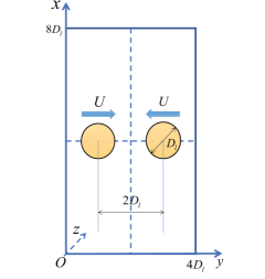
Figure 1: Geometrical configuration of head-on collision of two identical droplets. $D_{l}$ is the droplet diameter and $U$ is the initial droplet speed.

As a sensible first step to explore the rarefaction effects with a BGK-Boltzmann equation, the constant relaxation time is used in this research, which implies that the kinematic viscosity ratio $r_{\nu}\equiv\nu_{l}/\nu_{g}$ is always equal to the unity. Obviously, the density ratio $r_{\rho}\equiv\rho_{l}/\rho_{g}$ is always equal to the shear viscosity ratio $r_{\mu}\equiv\mu_{l}/\mu_{g}$, because $\nu=\mu/(\rho RT)$ holds for the present model. Since the simple double-well bulk free-energy density in (2) works as a good approximation only in the vicinity of the critical point of the equation of state (Jamet et al., 2001; Lee & Fischer, 2006), the range of the density ratio that can be handled by this approximation should not be arbitrarily exaggerated for different kinetic flow regimes. On the one hand, we have noticed that for continuum flows, a formulation for the order parameter similar to (2) can be applied to successfully simulate large-density-ratio ($r_{\rho}\geq 1000$) immiscible two-phase flows by coupling with the Cahn-Hilliard (CH) or Allen-Cahn (AC) equation and by using some stability-enhanced numerical techniques (Liang et al., 2018; Kumar et al., 2019), which drastically extends its theoretical limit. On the other hand, no results for its applicable density ratio are reported for non-continuum flows. Therefore, the small density ratio $r_{\rho}=2$ is considered in the present research without violating the theoretical limitation. Except for the viscosity and density ratios, the problem is also controlled by the conventional Weber number $We$ and the Reynolds number $Re$:

$$We=\frac{4\rho_{l}D_{l}U^{2}}{\sigma_{s}},\quad Re=\frac{2\rho_{l}D_{l}U}{\mu_{l}},$$ (41)

as well as the Knudsen number $Kn$

$$Kn=\frac{\sqrt{RT}\tau}{D_{l}}.$$ (42)

Usually, the continuum flow regime lies in the range $Kn\lesssim 0.001$. The non-continuum effects gradually become prominent as the Knudsen number increases. It is noted that $D_{l}$ in the denominator of (42) represents the maximum thickness of the interdroplet gas film when the droplets come to contact.

The interfacial thickness $W$ of each droplet occupies $4$ lattices, which satisfies the empirical condition $(W>3\Delta x)$ for numerically sustainable interface thickness (Lee & Fischer, 2006). It is mentioned that the following simulations are performed without applying extra numerical techniques such as the van Leer limiter or the weighted essentially non-oscillatory (WENO) scheme (van Leer, 1977; Jiang & Shu, 1996). All the spatial derivatives are evaluated using the second-order finite difference schemes at both the cell centres and the cell interfaces, which is consistent with the second-order spatial accuracy of the DUGKS. Therefore, with sufficient gird resolution, the artificial finite resolution effects inherent in these numerical schemes are believed to be constrained to such an extent that the critical physical information is not obviously contaminated.

Combining these careful numerical considerations, we believe that the present two-dimensional study could provide some new physical insights on higher-order non-continuum effects for head-on binary droplet collision problem.

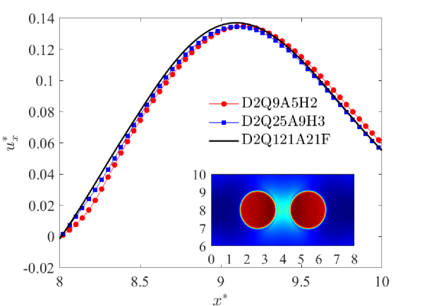
(a) $t^{*}=0.3$

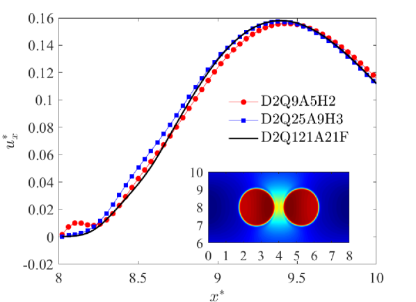
(b) $t^{*}=0.4$

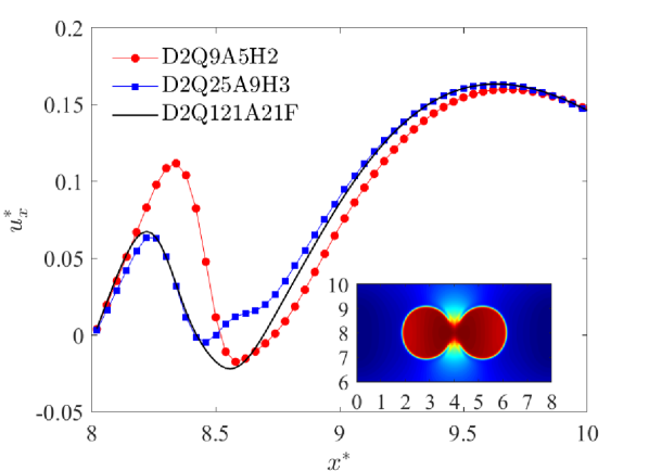
(c) $t^{*}=0.5$

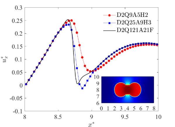
(d) $t^{*}=0.6$

Figure 2: Evolution of the normalized velocity component $u_{x}^{*}$ in the $x$-direction. (a) $t^{*}=0.3$, (b) $t^{*}=0.4$, (c) $t^{*}=0.5$ and (d) $t^{*}=0.6$. $We=1600$, $Re=13.33$ and $Kn=0.052$.

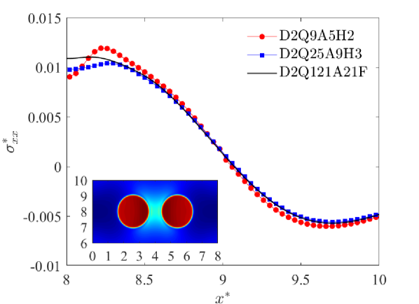
(a) $t^{*}=0.3$

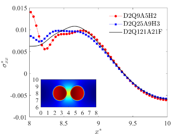
(b) $t^{*}=0.4$

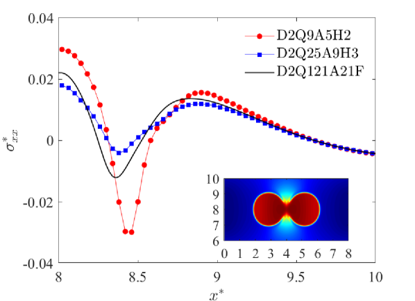
(c) $t^{*}=0.5$

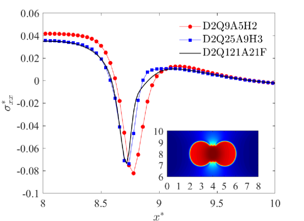
(d) $t^{*}=0.6$

Figure 3: Evolution of the normalized viscous stress $\sigma_{xx}^{*}$ in the $x$-direction. (a) $t^{*}=0.3$, (b) $t^{*}=0.4$, (c) $t^{*}=0.5$ and (d) $t^{*}=0.6$. $We=1600$, $Re=13.33$ and $Kn=0.052$.

4.2 Simulation results and discussions

4.2.1 $Kn=0.052$

We simulate a case with the dimensionless parameters: $We=1600$, $Re=13.33$ and $Kn=0.052$. The ratio of the time step to the relaxation time is $\Delta{t}/\tau\approx 0.011$ and that of the grid spacing to the mean free path is $\Delta{x}/\lambda\approx 0.19$, which implies that the kinetic scales have been fully resolved in the present simulation. The time in the following figures are normalized by $D_{l}/U$. Different Gauss-Hermite quadratures including D2Q9A5, D2Q25A9, D2Q81A17, D2Q121A21, D2Q169A25 and D2Q225A29 will be applied in the simulation. For neatness, not all the curves are presented in the following figures.

We mainly focus on the rarefaction effect during the formation of interdroplet gas film till the occurrence of coalescence. Coalescence happens if the interdroplet gas film can be squeezed out such that the contact point forms. The resistance with which the interdroplet gas film can be discharged depends on the droplet inertia as well as the dynamics of the film flow in particular to the pressure buildup within it (Qian & Law, 1997). On the one hand, the high Weber number in the present simulation guarantees that the high drop inertia can overcome the viscous dissipation, surface tension work and the lubrication resistance inside the interdroplet gas film, rendering the successful coalescence. On the other hand, the droplets with high impact inertia greatly squeeze out the intervening gas film to some extent, causing more appreciable spatial variations of observable quantities in a neighbourhood of the contact point.

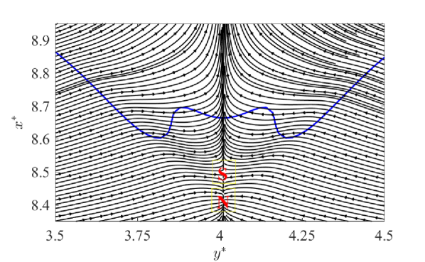
(a) D2Q25A9H3

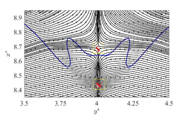
(b) D2Q121A21F

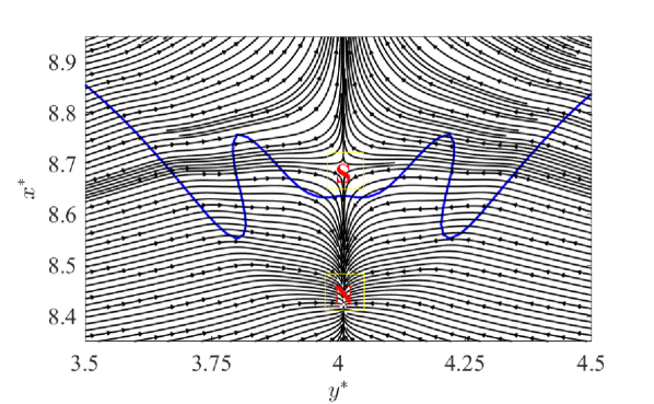
(c) D2Q169A25F

(d) D2Q225A29F

Figure 4: Streamlines at $t^{*}=0.5$, where the red-marked $N$ and $S$ represent the node and saddle points, respectively. The blue contour line denotes the density $\rho=(\rho_{l}+\rho_{g})/2$. (a) D2Q25A9H3; (b) D2Q121A21F; (c) D2Q169A25F; (d) D2Q225A29F. $We=1600$, $Re=13.33$ and $Kn=0.052$.

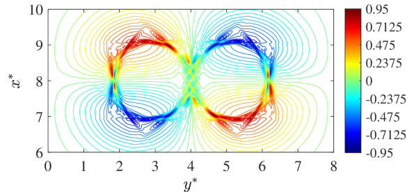
(a) D2Q25A9H3

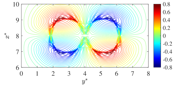
(b) D2Q121A21F

Figure 5: Contour of vorticity $\omega^{*}$ at $t^{*}=0.5$. (a) D2Q25A9H3 and (b) D2Q121A21F. $We=1600$, $Re=13.33$ and $Kn=0.052$.

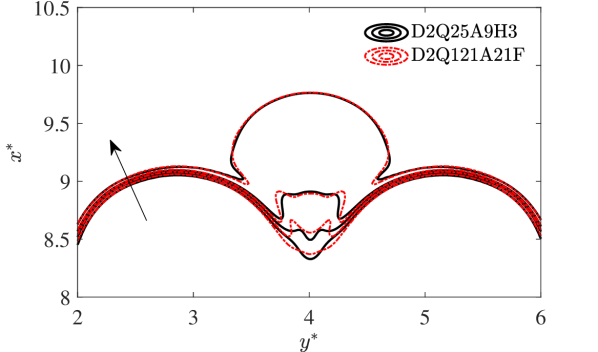
(a) $t^{*}=0.5$

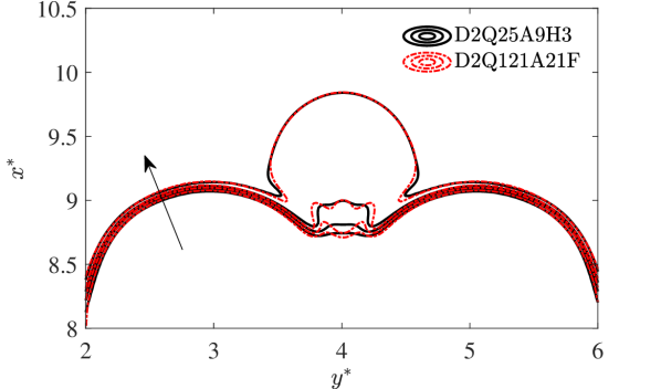
(b) $t^{*}=0.6$

Figure 6: Comparison of four dimensionless density profiles in the interfacial region of the droplets. Black: D2Q25A9H3, red: D2Q121A21F. The density decreases in the direction indicated by the arrow, where $\rho^{*}=0.75$, $0.90$, $1.05$ and $1.20$. (a) $t^{*}=0.5$ and (b) $t^{*}=0.6$. $We=1600$, $Re=13.33$ and $Kn=0.052$.

Figures 2 and 3 show the time evolutions of the normalized vertical velocity component $u_{x}^{*}\equiv u_{x}/U$ and the viscous stress component $\sigma_{xx}^{*}\equiv 2\sigma_{xx}/(\rho_{l}+\rho_{g})RT$ near the centreline of the interdroplet gas film (the left limiting position $y^{*}\rightarrow 4$). At $t^{*}=0.3$, the droplets are moving closer towards each other but are separated by a relatively long centre-to-centre distance. The interdroplet gas region is being compressed such that a monotonic increase of $u_{x}^{*}$ is observed till around $x^{*}=9$, followed by a monotonic decrease of the velocity magnitude. In figure 2b, the maximum value of the velocity magnitude increases at $t^{*}=0.4$ compared to that shown at $t^{*}=0.3$, because the interdroplet gas film is further compressed as the centre-to-centre distance between the droplets becomes shorter. In these two time instants, the rarefaction effect is not pronounced in the interdroplet gas region. Therefore, no obvious changes can be seen in the distributions of $u_{x}^{*}$ obtained from different Gauss-Hermite quadratures, except that an obvious variation of $\sigma_{xx}^{*}$ can be observed near $x^{*}=8$, as shown in figures 3a and 3b.

As illustrated in figures 2c and 3c, the liquid bridge forms at the coalescence region and the droplets are merging due to the attractive intermolecular force at $t^{*}=0.5$. Relatively large spatial variations of $u_{x}^{*}$ and $\sigma_{xx}^{*}$ are observed near the contact point in particular to the region around $x^{*}=8.5$. The differences between the results obtained using different Gauss-Hermite quadratures become pronounced compared to figures 3a and 3b. It is clear that both $u_{x}^{*}$ and $\sigma_{xx}^{*}$ converge with the increase of the number of discrete particle velocities. According to the analysis in Section 3.3, a Gauss-Hermite quadrature with at least $6^{th}$-order degree of precision is needed to compute the viscous stress tensor accurately at the Navier-Stokes order. Therefore, with the $3^{rd}$-order Hermite expansion for the equilibrium distribution function, D2Q25A9H3 has sufficient capability to capture the flow physics at the Navier-Stokes level, while incorporating the higher-order non-continuum effects is beyond its ability. Therefore, the differences between the results obtained by D2Q25A9H3 and higher-order Gauss-Hermite quadratures should be attributed to the rarefaction effect. Although the second-order Hermite expansion cannot ensure accurate evaluation of the viscous stress tensor at the Navier-Stokes order, it is noted that D2Q9A5H2 is usually applied to simulate the continuum flows in the conventional LBM. However, for this case with high impact inertia and approaching rate of two droplets, the viscous stress tensor cannot be accurately obtained using D2Q9A5H2, which will definitely influence the simulated droplet evolution process (see figures 2 and 3). Interestingly, D2Q9A5H2 still gives similar trends for the spatial variations of both $u_{x}^{*}$ and $\sigma_{xx}^{*}$ qualitatively. In contrast, higher-order Gauss-Hermite quadratures (D2Q81A17F, D2Q121A21F, D2Q169A25F and D2Q225A29F) can capture the non-continuum effects beyond the Navier-Stokes order to different levels. For this case, we find that D2Q81A17F can already give satisfying predictions with minor discrepancies which can be further reduced using D2Q121A21F. At the time $t^{*}=0.6$, the coalescence continues after the interdroplet gas film is forcibly discharged. The density in the merging region slightly arises and the rarefaction effect is attenuated compared to that observed at $t^{*}=0.5$. This can be further evidenced by figures 2d and 3d, where the differences between the results obtained from different Gauss-Hermite quadratures are not very prominent. The rarefaction effect mainly concentrates near the edge of the liquid bridge at $t^{*}=0.6$.

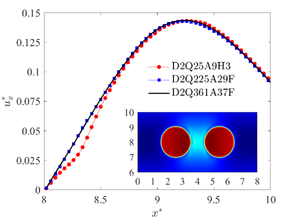
(a) $t^{*}=0.3$

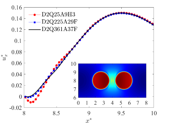
(b) $t^{*}=0.4$

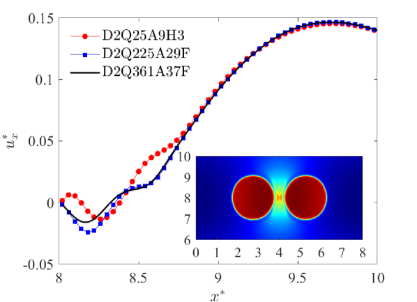
(c) $t^{*}=0.5$

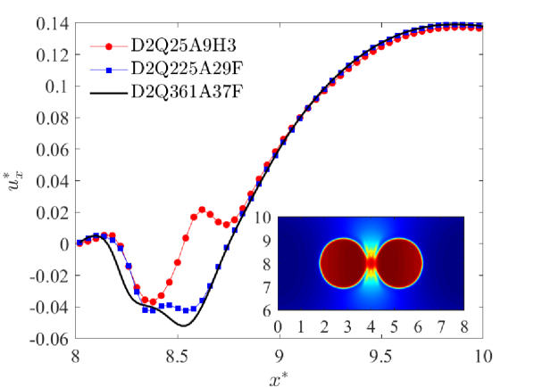
(d) $t^{*}=0.6$

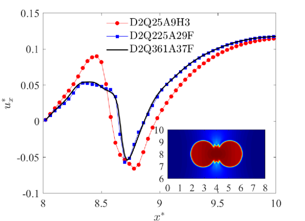
(e) $t^{*}=0.8$

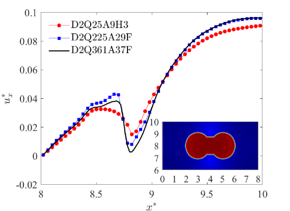
(f) $t^{*}=1.0$

Figure 7: Evolution of the normalized velocity component $u_{x}^{*}$ in the $x$-direction. (a) $t^{*}=0.3$, (b) $t^{*}=0.4$, (c) $t^{*}=0.5$, (d) $t^{*}=0.6$, (e) $t^{*}=0.8$, (f) $t^{*}=1.0$. $We=1600$, $Re=6.67$ and $Kn=0.104$.

To further demonstrate the rarefaction effect, figures 4 and 5 show the snapshots of the streamlines and the vorticity contours at $t^{*}=0.5$, respectively. In figure 4, the profiles of the merged droplet are superposed on the streamlines for comparison. Overall, the directions of the streamlines are consistent with our physical intuition. Interestingly, a more distinct saddle-node pair can be clearly identified in figures 4b, 4c and 4d when compared to that shown in figure 4a. On the one hand, from topological perspective, the resulting velocity field can be mapped onto a toroidal surface since the periodic boundary conditions are used in the simulations. The Poincaré–Bendixson (P-B) index theorem (Flegg, 2001) says that the number of nodes must be equal to the number of saddles for any smooth vector field on a toroidal surface. A careful examination of the whole velocity field shows that there are six nodes and six saddles (including those in figure 4) in the whole flow field, which implies the resulting streamline topology is reasonable (this also provides a self-consistent check for our calculation). On the other hand, D2Q121A21F, D2Q169A25F and D2Q225A29F can capture the higher-order non-continuum effect beyond the Navier-Stokes level, while D2Q25A9H3 can only pick up flow physics at the Navier-Stokes order. Therefore, the more distinct saddle-node pair and the relatively large crown structure are conjectured to be caused by the rarefaction effect. To some degree, since the present configuration is symmetrical with respect to the centreline $y^{*}=4$, the formation of these distinct flow structures could be comparable to those observed in droplet spreading and splash phenomena on a surface, which are already shown to be influenced by the rarefaction effect (Mandre & Brenner, 2012; Sprittles, 2015, 2017). The case shown here seems more complicated since the intervening liquid plane has more complex velocity and viscous stress variations compared to a stationary solid wall. In addition, due to the rarefaction effect, the vorticity concentration $\omega^{*}\equiv\omega/(2U/D_{l})$ around outer interfaces of the droplets is attenuated and the number of the sharp shear layers also decreases, as illustrated in figure 5. High-magnitude positive and negative vorticity centres in the interdroplet region are also suppressed. This could be related to the previous finding that the rarefaction effect can reduce the lubrication resistance force, facilitate the rupture of the interdroplet gas film and boost the droplet coalescence (Gopinath et al., 1997; Li, 2016).

Figure 6 compares the dimensionless density profiles $\rho^{*}\equiv 2\rho/(\rho_{l}+\rho_{g})$ obtained from D2Q25A9H3 and D2Q121A21F in the interfacial region of the droplets, respectively. It is observed that the rarefaction effect mainly influences the density profiles between the two droplets while the outer density profiles overlap very well. It is also seen that the region with obvious discrepancies in the density profiles has prominent variations of the vertical velocity component $u_{x}^{*}$ (figure 2) and the viscous stress component $\sigma_{xx}^{*}$ (figure 3).

4.2.2 $Kn=0.104$

Next, we simulate a case with higher Knudsen number: $We=1600$, $Re=6.67$ and $Kn=0.104$. The ratio of the time step to the relaxation time is $\Delta{t}/\tau\approx 0.0056$ and that of the grid spacing to the mean free path is $\Delta{x}/\lambda\approx 0.096$. Figures 7 and 8 show the time evolutions of the normalized vertical velocity component $u_{x}^{*}\equiv u_{x}/U$ and the viscous stress component $\sigma_{yy}^{*}\equiv 2\sigma_{yy}/(\rho_{l}+\rho_{g})RT$ near the centreline of the interdroplet gas film (the left limiting position $y^{*}\rightarrow 4$). Owing to the higher Knudsen number, more discrete particle velocities are required to obtain the final convergent solution. It is observed that even the simulations with D2Q225A29F cannot give the final convergent solution during the evolution process. In contrast, D2Q361A37F and D2Q441A41F can capture almost all the higher-order non-continuum effects and therefore generate the satisfying convergent solution.

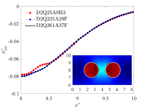
(a) $t^{*}=0.3$

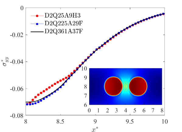
(b) $t^{*}=0.4$

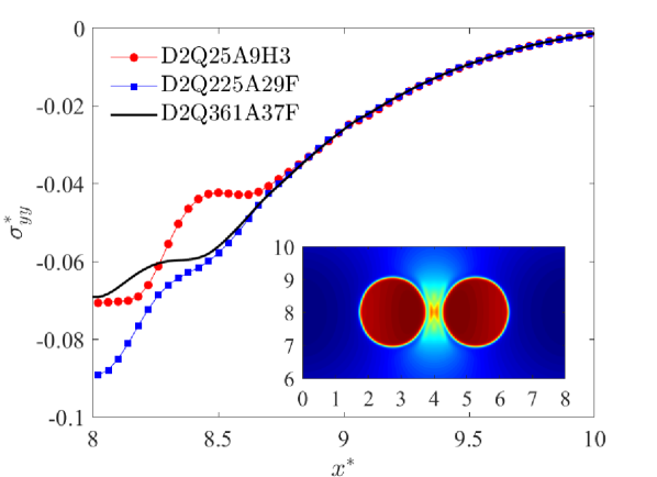
(c) $t^{*}=0.5$

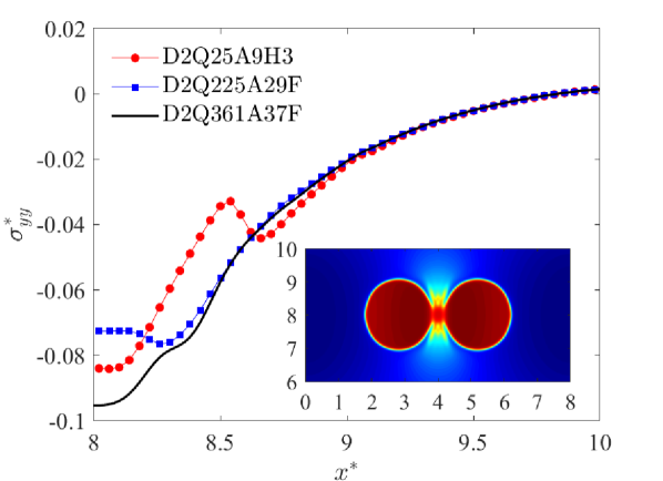
(d) $t^{*}=0.6$

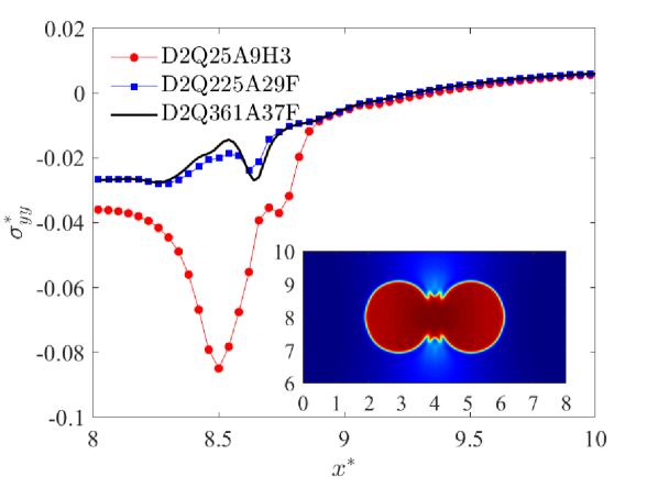
(e) $t^{*}=0.8$

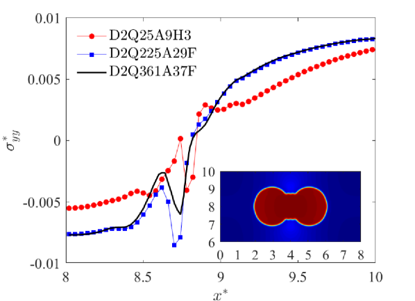
(f) $t^{*}=1.0$

Figure 8: Evolution of the normalized viscous stress $\sigma_{yy}^{*}$ in the $x$-direction. (a) $t^{*}=0.3$, (b) $t^{*}=0.4$, (c) $t^{*}=0.5$, (d) $t^{*}=0.6$, (e) $t^{*}=0.8$, (f) $t^{*}=1.0$. $We=1600$, $Re=6.67$ and $Kn=0.104$.

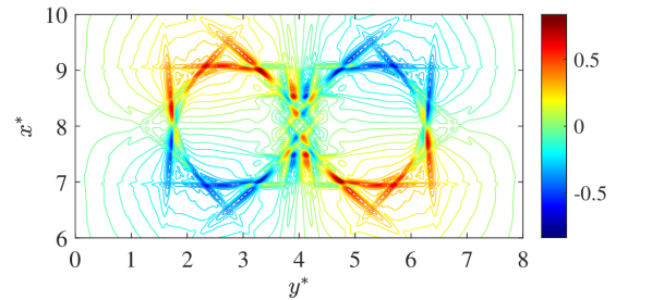
(a) D2Q25A9H3

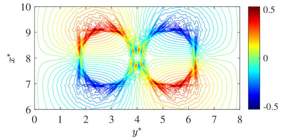
(b) D2Q361A37F

Figure 9: Contour of vorticity $\omega^{*}$ at $t^{*}=0.6$. (a) D2Q25A9H3 and (b) D2Q361A37F. $We=1600$, $Re=6.67$ and $Kn=0.104$.

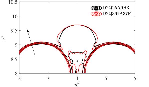
(a) $t^{*}=0.5$

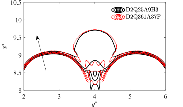
(b) $t^{*}=0.6$

Figure 10: Comparison of four dimensionless density profiles in the interfacial region of the droplets. Black: D2Q25A9H3, red: D2Q361A37F. The density decreases in the direction indicated by the arrow, where $\rho^{*}=0.75$, $0.90$, $1.05$ and $1.20$. (a) $t^{*}=0.5$ and (b) $t^{*}=0.6$. $We=1600$, $Re=6.67$ and $Kn=0.104$.

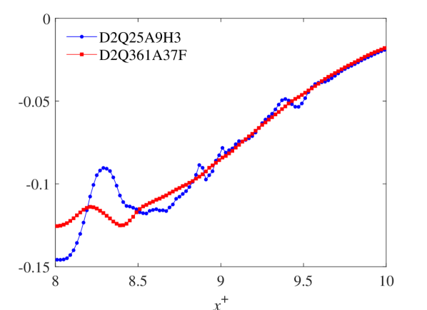
(a) $t^{*}=0.3$

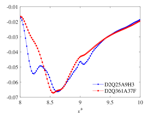
(b) $t^{*}=0.4$

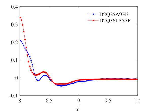
(c) $t^{*}=0.5$

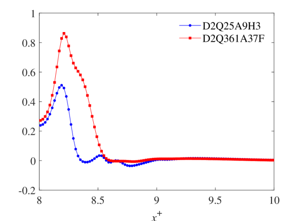
(d) $t^{*}=0.6$

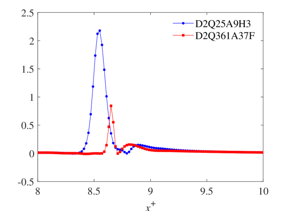
(e) $t^{*}=0.8$

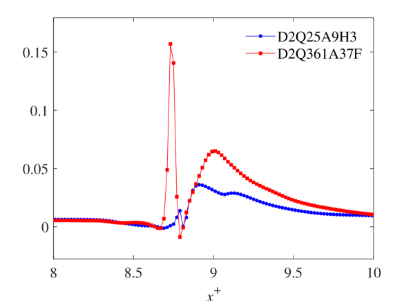
(f) $t^{*}=1.0$

Figure 11: Evolution of $T_{1}^{*}$ at $y^{*}=4$. (a) $t^{*}=0.3$, (b) $t^{*}=0.4$, (c) $t^{*}=0.5$, (d) $t^{*}=0.6$, (e) $t^{*}=0.8$, (f) $t^{*}=1.0$. $We=1600$, $Re=6.67$ and $Kn=0.104$.

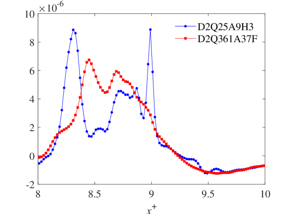
(a) $t^{*}=0.3$

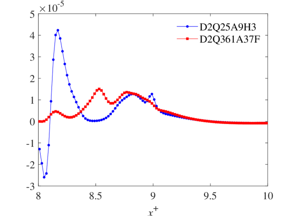
(b) $t^{*}=0.4$

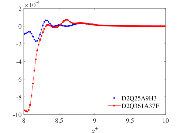
(c) $t^{*}=0.5$

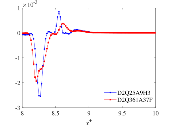
(d) $t^{*}=0.6$

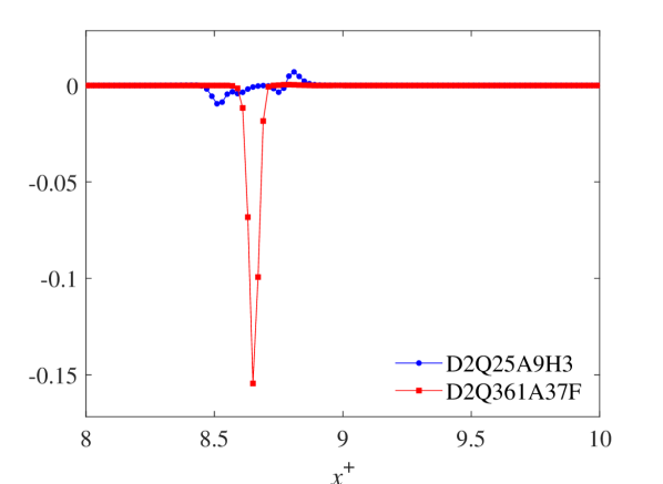
(e) $t^{*}=0.8$

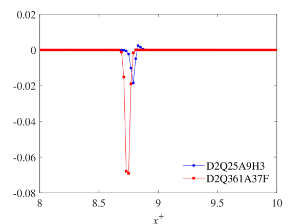
(f) $t^{*}=1.0$

Figure 12: Evolution of $T_{2}^{*}$ at $y^{*}=4$. (a) $t^{*}=0.3$, (b) $t^{*}=0.4$, (c) $t^{*}=0.5$, (d) $t^{*}=0.6$, (e) $t^{*}=0.8$, (f) $t^{*}=1.0$. $We=1600$, $Re=6.67$ and $Kn=0.104$.

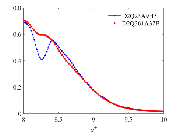
(a) $t^{*}=0.3$

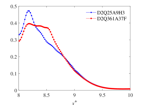
(b) $t^{*}=0.4$

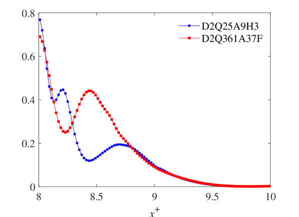
(c) $t^{*}=0.5$

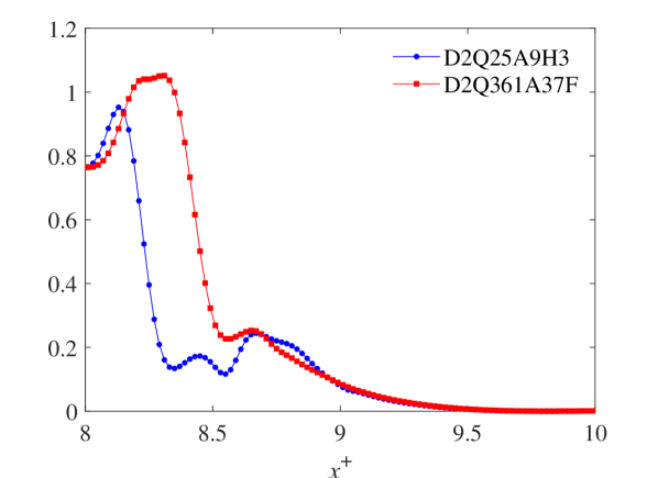
(d) $t^{*}=0.6$

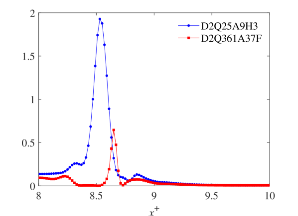
(e) $t^{*}=0.8$

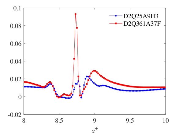
(f) $t^{*}=1.0$

Figure 13: Evolution of $T_{3}^{*}$ at $y^{*}=4$. (a) $t^{*}=0.3$, (b) $t^{*}=0.4$, (c) $t^{*}=0.5$, (d) $t^{*}=0.6$, (e) $t^{*}=0.8$, (f) $t^{*}=1.0$. $We=1600$, $Re=6.67$ and $Kn=0.104$.

At $t^{*}=0.3$ and $t^{*}=0.4$, different Gauss-Hermite quadratures give similar results since the interdroplet gas film is only slightly compressed. As the droplets approach each other ($t^{*}=0.5$, $0.6$ and $0.8$), the lubrication layer between the droplets gradually forms until the emergence of the liquid bridge. It is clearly observed that the discrepancies between the results obtained from D2Q25A9H3 and those from other higher-order Gauss-Hermite quadratures become pronounced, particularly in the region from $x^{*}=8$ to $x^{*}=9$ (about one droplet radius). At $t^{*}=0.8$, a highly negative peak region is observed for D2Q25A9H3, which is suppressed due to the rarefaction effect. At $t^{*}=1.0$, a liquid bridge connecting the two droplets is formed. The discrepancies caused by the rarefaction effect can still be observed because the gas at the flank of the liquid bridge is still being squeezed out due to the movement of the droplets.

Figure 9 shows the normalized snapshots of the vorticity $\omega^{*}$ at $t^{*}=0.6$. Compared to the case where $Kn=0.052$, the vorticity distribution is significantly changed by the rarefaction effect. On the one hand, high-magnitude positive and negative vorticity centres around the interface are considerably diffused to form round regions, making the vorticity distribution more uniform there. One the other hand, the vorticity concentration inside the interdroplet region is also depleted as the coalescence occurs.

Figure 10 compares the dimensionless density profiles $\rho^{*}\equiv 2\rho/(\rho_{l}+\rho_{g})$ obtained from D2Q25A9H3 and D2Q361A37F in the interfacial region of the droplets, respectively. Compared to the case with $Kn=0.052$, the density structures between the two droplets are significantly changed by the enhanced higher-order non-continuum effects.

4.2.3 Rarefaction effects on energy conversion and viscous dissipation

Although the rarefaction effects in the gas film have been noticed and described in several existing studies (Zhang & Law, 2011; Li, 2016; Sprittles, 2015, 2017), rarefaction effects on energy conversion and droplet coalescence are not explored yet. For the present model, the total energy is the sum of the kinetic energy and the free energy. Therefore, we first present a general derivation for the evolution equations of the free and kinetic energies in order to theoretically reveal the energy conversion mechanisms between these two energies. Then, rarefaction effects on relevant energy conversion terms are discussed using the simulation data. It is mentioned that the following derivation is general and does not depend on the specific form of the bulk free energy density $\psi$, and hence the equation of state $p_{0}$.

The free energy density $f_{e}$ is a single-valued function of two variables $\rho$ and $\bm{\nabla}\rho$, namely,

$$f_{e}(\rho,\bm{\nabla}\rho)=\psi(\rho)+\frac{1}{2}\kappa\lVert\bm{\nabla}\rho\rVert^{2}.$$ (43)

By applying the chain rule for the material derivative of $f_{e}$, we obtain

$$\frac{Df_{e}}{Dt}=\frac{\partial f_{e}}{\partial\rho}\frac{D\rho}{Dt}+\frac{\partial f_{e}}{\partial\bm{\nabla}\rho}\bm{\cdot}\frac{D\bm{\nabla}\rho}{Dt},$$ (44)

The partial derivatives of $f_{e}$ with respect to $\rho$ and $\bm{\nabla}\rho$ are $\partial{f_{e}}/\partial\rho=\mu_{0}$ and ${\partial f_{e}}/{\partial\bm{\nabla}\rho}=\kappa\bm{\nabla}\rho$, respectively. Using (12), the material derivatives of $\rho$ and $\bm{\nabla}\rho$ are respectively evaluated as

$$\frac{D\rho}{Dt}=\frac{\partial\rho}{\partial t}+\bm{u}\bm{\cdot}\bm{\nabla}\rho=-\rho\vartheta,$$ (45)

and

$$\frac{D\bm{\nabla}\rho}{Dt}=\bm{\nabla}\frac{\partial\rho}{\partial t}+\bm{u}\bm{\cdot}\bm{\nabla\nabla}\rho=-\bm{\nabla}(\rho\vartheta)-\bm{\nabla}\rho\bm{\cdot}\bm{\nabla}\bm{u},$$ (46)

where $\vartheta\equiv\bm{\nabla}\bm{\cdot}\bm{u}$ represents the fluid dilatation. Substituting (45) and (46) into (44) gives

$$\frac{Df_{e}}{Dt} = -\rho\mu_{0}\vartheta-\kappa\lVert\bm{\nabla}\rho\rVert^{2}\vartheta-\kappa\rho\bm{\nabla}\rho\bm{\cdot}\bm{\nabla}\vartheta-{\kappa}\bm{\nabla}\rho\bm{\nabla}\rho\bm{:}\bm{S}$$ (47)

$$= -\rho\mu_{\rho}\vartheta-\kappa\lVert\bm{\nabla}\rho\rVert^{2}\vartheta-\kappa\rho\bm{\nabla}\bm{\cdot}\left(\vartheta\bm{\nabla}\rho\right)-{\kappa}\bm{\nabla}\rho\bm{\nabla}\rho\bm{:}\bm{S}$$

$$= -\rho\mu_{\rho}\vartheta-\bm{\nabla}\bm{\cdot}\left(\kappa\rho\vartheta\bm{\nabla}\rho\right)-{\kappa}\bm{\nabla}\rho\bm{\nabla}\rho\bm{:}\bm{S}.$$

Therefore, we have the evolution equation for $f_{e}$ as

$$\frac{\partial f_{e}}{\partial t}+\bm{u}\bm{\cdot}\bm{\nabla}f_{e}=-\rho\mu_{\rho}\vartheta-\bm{\nabla}\bm{\cdot}\left(\kappa\rho\vartheta\bm{\nabla}\rho\right)-{\kappa}\bm{\nabla}\rho\bm{\nabla}\rho\bm{:}\bm{S}.$$ (48)

Using the following relation,

$$\bm{u}\bm{\cdot}\bm{\nabla}f_{e}=\bm{\nabla}\bm{\cdot}(f_{e}\bm{u})-f_{e}\vartheta,$$ (49)

(48) can be rewritten as

$$\frac{\partial f_{e}}{\partial t}=-(\rho\mu_{\rho}-f_{e})\vartheta-\bm{\nabla}\bm{\cdot}\left(\kappa\rho\vartheta\bm{\nabla}\rho+f_{e}\bm{u}\right)-{\kappa}\bm{\nabla}\rho\bm{\nabla}\rho:\bm{S}.$$ (50)

Interestingly, using (3), (4), (25) and (43), we have

$$\rho\mu_{\rho}-f_{e} = \rho\left(\frac{\partial\psi}{\partial\rho}-\kappa\nabla^{2}\rho\right)-\left(\psi+\frac{1}{2}\kappa\lVert\bm{\nabla}\rho\rVert^{2}\right)$$ (51)

$$= \left(\rho\frac{\partial\psi}{\partial\rho}-\psi\right)-\kappa\rho\nabla^{2}\rho-\frac{1}{2}\kappa\lVert\bm{\nabla}\rho\rVert^{2}$$

$$= p_{0}-\kappa\rho\nabla^{2}\rho-\frac{1}{2}\kappa\lVert\bm{\nabla}\rho\rVert^{2}$$

$$= p,$$

which indicates that the difference between the chemical potential per unit volume and the free energy density is equal to the nonlocal total pressure, see (25). Then, combining (50) and (51) yields

$$\frac{\partial f_{e}}{\partial t}=-\bm{\nabla}\bm{\cdot}\left(\kappa\rho\vartheta\bm{\nabla}\rho+f_{e}\bm{u}\right)-T_{1}-T_{2},$$ (52)

where

$$T_{1}\equiv p\vartheta,~{}T_{2}\equiv{\kappa}\bm{\nabla}\rho\bm{\nabla}\rho\bm{:}\bm{S}.$$ (53)

In the right hand side of (52), the divergence term only contributes to the local variation of the free energy density but has no contribution to the energy conversion. $T_{1}$ represents the coupling between the total pressure and the dilatation. For the isosurface of the density field, $T_{2}$ can be rewritten as

$$T_{2}=\kappa\lVert\bm{\nabla}\rho\rVert^{2}\left(\vartheta-\frac{1}{S_{0}}\frac{dS_{0}}{dt}\right),$$ (54)

which represents the contribution to the temporal evolution rate of the free energy density through the dilatational process and the stretching/compression of the small material surface element $S_{0}$ on the isosurface of the density field.

Similarly, the evolution equation for the kinetic energy density $\rho u^{2}/2$ can be derived as

$$\frac{\partial}{\partial t}\left(\frac{1}{2}\rho u^{2}\right)=-\bm{\nabla}\bm{\cdot}\left(\bm{P}\bm{\cdot}\bm{u}-\bm{\sigma}\bm{\cdot}\bm{u}+\frac{1}{2}\rho u^{2}\bm{u}\right)+T_{1}+T_{2}-T_{3},$$ (55)

where

$$T_{3}\equiv\bm{\sigma}\bm{:}\bm{S}.$$ (56)

It follows from (52) and (55) that the local energy conversion between the free energy and the kinetic energy can only be realized through two physical mechanisms, namely, the coupling between the total pressure and the dilatation ($T_{1}$), and the interaction between the density gradient and the strain rate tensor ($T_{2}$). $T_{1}>0$ or $T_{2}>0$ represents the local conversion of the free energy into the kinetic energy. Conversely, the kinetic energy is locally converted to the free energy when $T_{1}<0$ or $T_{2}<0$. $T_{3}$ represents the viscous dissipation of the kinetic energy. We focus on the case with $Kn=0.104$ in the following discussion. $T_{1}$, $T_{2}$ and $T_{3}$ will be normalized by $\rho_{l}U^{3}/D_{l}$ for all the plots below.

Of particular interest are the rarefaction effects on local energy conversion and viscous dissipation along the vertical centreline $y^{*}=4$ where the gas film is squeezed out. Figure 11 shows the time evolution of $T_{1}^{*}$ along $y^{*}=4$. At $t^{*}=0.3$ and $t^{*}=0.4$ (figures 11a and 11b), the overall tendency of the results obtained from D2Q25A9H3 is similar to those from D2Q361A37F. Compared to D2Q25A9H3, the oscillations in the results of D2Q361A37F are suppressed due to the high-order non-continuum effect, in particular to those around $x^{*}=8$. Negative $T_{1}^{*}$ contributes to the local conversion of the kinetic energy to the free energy. At $t^{*}=0.5$ and $t^{*}=0.6$ (figures 11c and 11d), $T_{1}^{*}$ basically shows positive values near $x^{*}=0.8$, which indicates that the free energy is locally converted to the kinetic energy. Comparison of the results from D2Q25A9H3 and D2Q361A37F shows that this local energy conversion is enhanced by the rarefaction effect. At $t^{*}=0.8$ and $t^{*}=1.0$ (figures 11e and 11f), the liquid bridge is formed and the rarefaction effect mainly concentrates near its surface.

Figure 12 shows the time evolution of $T_{2}^{*}$ along $y^{*}=4$. One common feature for the evolution of $T_{1}^{*}$ and $T_{2}^{*}$ is that the rarefaction effect suppresses the oscillation magnitude of $T_{1}^{*}$ and $T_{2}^{*}$ at $t^{*}=0.3$ and $t^{*}=0.4$, as shown in figures 12a and 12b. At $t^{*}=0.5$ (figure 12c), a highly negative peak region is observed for D2Q361A37F, which locally contributes to the conversion of the kinetic energy to the free energy. However, the final energy conversion rate between the kinetic energy and the free energy is determined by the competition between $T_{1}^{*}$ and $T_{2}^{*}$. It is obvious that for the present case, the magnitude of $T_{2}^{*}$ is much lower than $T_{1}^{*}$, which implies the dominance of $T_{1}^{*}$ in the local energy conversion. Subsequently, the differences between the results from D2Q25A9H3 and D2Q361A37F for $T_{2}^{*}$ mainly concentrate near the surface of the liquid bridge, as displayed in figures 12d, 12e and 12f.

Furthermore, the time evolution of $T_{3}^{*}$ is displayed in figure 13. It is observed that $T_{3}^{*}$ basically remains positive, whose sign is not significantly changed by the high-order contribution $\bm{\sigma}^{(H)}\bm{:}\bm{S}$. At $t^{*}=0.3$ (figure 13a), the magnitude of $T_{3}^{*}$ obtained by D2Q361A37F is comparable to that from D2Q25A9H3. In comparison, no obvious oscillations are observed for D2Q361A37F near the collision point $x^{*}=8$. At $t^{*}=0.4$ (figure 13b), due to the rarefaction effect, the high magnitude region of $T_{3}^{*}$ is depleted along with a wider spatial distribution. In figures 13c and 13d, compared to D2Q25A9H3, higher viscous dissipation rate can be observed for D2Q361A37F near the collision point. This is reasonable since the enhanced pressure-dilatation coupling effect in the same region converts more free energy to kinetic energy, causing the growth of the viscous dissipation rate. The characteristic of the distribution of $T_{3}^{*}$ is similar to those of $T_{1}^{*}$ and $T_{2}^{*}$, which is also concentrated near the surface of the liquid bridge (figures 13e and 13f).

5 Conclusions and discussions

In this paper, in order to investigate the rarefaction effects in head-on collision of two identical droplets, two DUGKS simulations with the Knudsen numbers $Kn=0.052$ and $0.104$ are performed based on a BGK-Boltzmann equation. The main findings and contributions are summarised as follows.

(a) We observe the rarefaction effects during the binary droplet collision by using the Gauss-Hermite quadratures with different degree of precision. The convergent solutions are obtained by gradually increasing the number of discrete particle velocities for both the simulated cases. For the case with $Kn=0.052$, D2Q81A17F is sufficient to obtain the satisfying convergent solution. In contrast, D2Q361A37F is needed to capture the higher-order non-continuum effects for the case with $Kn=0.104$.

(b) We analyse the rarefaction effects on the time evolution of the binary droplet collision event. The spatial distribution of the vertical velocity (hence the droplet morphology) and the viscous stress components are found to be influenced by the non-continuum effects during the formation of the liquid bridge. The topology of streamlines near the droplets’ surface is significantly altered due to the rarefaction effect. For example, a saddle-node pair and a relatively large crown structure are observed for $Kn=0.052$, which is very similar to the flow structure and surface configuration previously observed in droplet spreading and splash on a solid surface associated with the rarefaction effects (Mandre & Brenner, 2012; Sprittles, 2015, 2017). In addition, high-magnitude vorticity concentration in the interdroplet region is observed to be suppressed, which is related to the previous finding that the rarefaction effect can boost the droplet coalescence (Gopinath et al., 1997; Li, 2016). The rarefaction effect also promotes the vorticity diffusion around the outer droplet surface, making the vorticity distribution more uniform there. Moreover, it is observed the the spatial structures of the density field between the droplets are significantly changed by the rarefaction effects.

(c) We provide a detailed analysis for the rarefaction effects on energy conversion and viscous dissipation. For the present model, we mathematically prove that only two physical mechanisms are responsible for the energy conversion between the kinetic energy and the free energy, namely the pressure-dilatation coupling effect $T_{1}\equiv p\vartheta$ and the interaction between the density gradient and the strain rate tensor $T_{2}\equiv\kappa\bm{\nabla}\rho\bm{\nabla}\rho\bm{:}\bm{S}$, where the nonlocal total pressure $p$ is given in (25). Therefore, the final energy conversion rate depends on the competition between $T_{1}$ and $T_{2}$ in different flow problems. For the case with $Kn=0.104$, it is found that $T_{1}$ dominates the energy conversion from the free energy to the kinetic energy, which facilitates the discharge of the interdroplet gas film along the vertical direction and boosts the coalescence of two droplets. We show that this characteristic is enhanced by the rarefaction effect, which is accompanied by the enhancement of the viscous dissipation rate ($T_{3}\equiv\bm{\sigma}\bm{:}\bm{S}$) near the surface of the liquid bridge.

Extended studies could be carried out to explore the physical mechanisms associated with different dimensionless parameters, which could provide new insights into the rarefaction effects on binary droplet collision dynamics and outcomes. The present code can be modified to investigate the rarefaction effects in non-continuum physical phenomena including moving contact line, boiling and cavitation. For example, when the size of the bubble is comparable to the mean free path of the gas, the rarefaction effects are likely to dominate the local dynamic behaviour of the bubble. For these problems, the kinetic equation could provide a more physical framework to incorporate the higher-order rarefaction effects compared to the modified Navier-Stokes equation.

Declaration of interests

The authors report no conflict of interest.

References

- Anderson et al. (1998) Anderson, D. M., McFadden, G. B. & Wheeler, A. A. 1998 Diffuse-interface methods in fluid mechanics. Annu. Rev. Fluid Mech. 30, 1.
- Ashgriz & Poo (1990) Ashgriz, N. & Poo, J. Y. 1990 Coalescence and separation in binary collisions of liquid drops. J. Fluid Mech. 221, 183–204.
- Beilharz et al. (2015) Beilharz, D., Guyon, A., Li, E. Q., Thoroval, M.-J. & Thoroddsen, S. T. 2015 Antibubbles and fine cylindrical sheets of air. J. Fluid Mech. 779, 87.
- Benilov & Benilov (2018) Benilov, E. S. & Benilov, E. S. 2018 Energy conservation and H theorem for the Enskog-Vlasov equation. Phys. Rev. E 97, 062115.
- Benilov & Benilov (2019) Benilov, E. S. & Benilov, M. S. 2019 Peculiar property of noble gases and its explanation through the Enskog-Vlasov model. Phys. Rev. E 99, 012144.
- Bhatnagar et al. (1954) Bhatnagar, P. L., Gross, E. P. & Krook, M. 1954 A Model for Collision Processes in Gases. I. Small Amplitude Processes in Charged and Neutral One-Component Systems. Phys. Rev. 94 (3), 511–525.
- Busuioc et al. (2020) Busuioc, S., Gibelli, L., Lockerby, D. A. & Sprittles, J. E. 2020 Velocity distribution function of spontaneously evaporating atoms. Phys. Rev. Fluids 5, 10.
- Cahn & Hilliard (1958) Cahn, J. W. & Hilliard, J. E. 1958 Free Energy of a Nonuniform System. I. Interfacial Free Energy. J. Chem. Phys. 28 (2), 258–267.
- Carnahan & Starling (1969) Carnahan, N. F. & Starling, K. E. 1969 Equation of State for Nonattracting Rigid Spheres. J. Chem. Phys. 51 (2), 635–636.
- Chapman & Cowling (1970) Chapman, S. & Cowling, T. G. 1970 The Mathematical Theory of Non-uniform Gases. Cambridge: Cambridge University.
- Chen & Doolen (1998) Chen, S. & Doolen, G. D. 1998 Lattice Boltzmann method for fluid flows. Annu. Rev. Fluid Mech. 30 (1), 329–364.
- Chen & Yang (2020) Chen, X. & Yang, V. 2020 Direct numerical simulation of multiscale flow physics of binary droplet collision. Phys. Fluids 32, 062103.
- Flegg (2001) Flegg, H. G. 2001 From geometry to topology. New York: Dover publications.
- Frezzotti et al. (2018) Frezzotti, A., Gibelli, L., Lockerby, D. A. & Sprittles, J. E. 2018 Mean-field kinetic theory approach to evaporation of a binary fluid into vacuum. Phys. Rev. Fluids 3, 054001.
- Frezzotti et al. (2005) Frezzotti, A., Gibelli, L. & Lorenzani, S. 2005 Mean field kinetic theory description of evaporation of a fluid into vacuum. Phys. Fluids 17, 012102.
- Gibelli et al. (2015) Gibelli, L., Frezzotti, A. & Barbante, P. 2015 A kinetic theory description of liquid menisci at the microscale. Kinetic & related models 8 (2), 235–254.
- Gopinath et al. (1997) Gopinath, A., Chen, S. B. & Koch, D. L. 1997 Lubrication flows between spherical particles colliding in a compressible non-continuum gas. J. Fluid Mech. 344, 245–269.
- Grad (1949) Grad, H. 1949 Note on N-dimensional Hermite polynomials. Commun. Pure Appl. Math. 2, 325.
- Gunstensen et al. (1991) Gunstensen, A. K., Rothman, D. H., Zaleski, S. & Zanetti, G. 1991 Lattice Boltzmann model of immiscible fluids. Phys. Rev. A 43 (8), 4320–4327.
- Guo (2021) Guo, Z. 2021 Well-balanced lattice Boltzmann model for two-phase systems. Phys. Fluids 33, 031709.
- Guo et al. (2013) Guo, Z., Xu, K. & Wang, R. 2013 Discrete unified gas kinetic scheme for all Knudsen number flows: Low-speed isothermal case. Phys. Rev. E 88, 033305.
- Guo et al. (2005) Guo, Z., Zhao, T. S. & Shi, Y. 2005 Simple kinetic model for fluid flows in the nanometer scale. Phys. Rev. E 71 (3), 035301.
- He et al. (2019) He, C., Xia, X. & Zhang, P. 2019 Non-monotonic viscous dissipation of bouncing droplets undergoing off-center collision. Phys. Fluids 31, 052004.
- He & Zhang (2020) He, C. & Zhang, P. 2020 Non-axisymmetric flow characteristics in head-on collision of spinning droplets. Phys. Rev. Fluids 5, 113601.
- He et al. (1999) He, X., Chen, S. & Zhang, R. 1999 A lattice Boltzmann scheme for incompressible multiphase flow and its application in simulation of Rayleigh-Taylor instability. J. Comput. Phys. 152 (2), 642–663.
- He & Doolen (2002) He, X. & Doolen, G. D. 2002 Thermodynamic Foundations of Kinetic Theory and Lattice Boltzmann Models for Multiphase Flows. J. Stat. Phys. 107 (112), 309–328.
- Huang et al. (2021) Huang, R., Wu, H. & Adams, N. A. 2021 Mesoscopic Lattice Boltzmann Modeling of the Liquid-Vapor Phase Transition. Phys. Rev. Lett. 126 (24), 244501.
- Jacqmin (1999) Jacqmin, D. 1999 Calculation of two-phase Navier-Stokes flows using phase-field modeling. J. Comput. Phys. 15 (1), 96–127.
- Jacqmin (2000) Jacqmin, D. 2000 Contact-line dynamics of a diffuse fluid interface. J. Fluid Mech. 402, 57–88.
- Jamet et al. (2001) Jamet, D., Lebaigue, O., Coutris, N. & Delhaye, J. M. 2001 The second gradient theory: a tool for the direct numerical simulation of liquid-vapor flows with phase-change. Nucl. Eng. Technol. 204, 155–166.
- Jiang & Shu (1996) Jiang, G.-S. & Shu, C.-W. 1996 Efficient implementation of weighted ENO schemes. J. Comput. Phys. 126 (1), 202 – 228.
- Jiang & James (2007) Jiang, X. & James, A. J. 2007 Numerical simulation of the head-on collision of two equal-sized drops with van der Waals forces. J. Eng. Math. 59, 99.
- Jiang et al. (1992) Jiang, Y. J., Umemura, A. & Law, C. K. 1992 An experimental investigation on the collision behaviour of hydrocarbon droplets. J. Fluid Mech. 234, 171.
- Kobayashi et al. (2017) Kobayashi, K., Sasaki, K., Kon, M., Fujii, H. & Watanabe, M. 2017 Kinetic boundary conditions for vapor-gas binary mixture. Microfluid. Nanofluid. 21, 53.
- Kon et al. (2014) Kon, M., Kobayashi, K. & Watanabe, M. 2014 Method of determining kinetic boundary conditions in net evaporation/condensation. Phys. Fluids 26 (7), 072003.
- Kremer & Rosa (1988) Kremer, G. M. & Rosa, E. 1988 On Enskog’s dense gas theory. I: The method of moments for monatomic gases. J. Chem. Phys. 89 (5), 3240–3247.
- Kumar et al. (2019) Kumar, E. D., Sannasiraj, S. A. & Sundar, V. 2019 Phase field lattice Boltzmann model for airwater two phase flows. Phys. Fluids 31, 072103.
- Lee & Fischer (2006) Lee, Taehun & Fischer, P. F. 2006 Eliminating parasitic currents in the lattice Boltzmann equation method for nonideal gases. Phys. Rev. E 74, 046709.
- van Leer (1977) van Leer, B. 1977 Towards the ultimate conservative difference scheme. IV. A new approach to numerical convection. J. Comput. Phys. 23, 276 – 299.
- Li (2016) Li, J. 2016 Macroscopic model for head-on binary droplet collisions in a gaseous medium. Phys. Rev. Lett. 117, 214502.
- Li et al. (2020) Li, Q., Yu, Y. & Wen, Z. X. 2020 How does boiling occur in lattice Boltzmann simulations? Phys. Fluids 32, 093306.
- Liang et al. (2018) Liang, H., Xu, J., Chen, J., Wang, H., Chai, Z. & Shi, B. 2018 Phase-field-based lattice Boltzmann modeling of large-density-ratio two-phase flows. Phys. Rev. E 97, 033309.
- Luo (2000) Luo, L. S. 2000 Theory of the lattice Boltzmann method: Lattice Boltzmann models for nonideal gases. Phys. Rev. E 62 (4), 4982–4996.
- Mandre & Brenner (2012) Mandre, S. & Brenner, M. P. 2012 The mechanism of a splash on a dry solid surface. J. Fluid Mech. 690, 148–172.
- Nobari et al. (1996) Nobari, M. R., Jan, Y.-J. & Tryggvason, G. 1996 Head-on collision of drops–a numerical investigation. Phys. Fluids 8, 29–42.
- Orme (1997) Orme, M. 1997 Experiments on droplet collisions, bounce, coalescence and disruption. Prog. Energy Combust. Sci. 23, 65.
- Pan et al. (2009) Pan, K.-L., Chou, P. C. & Tseng, Y.-J. 2009 Binary droplet collision at high Weber number. Phys. Rev. E 80, 036301.
- Pan et al. (2008) Pan, K.-L., Law, C. K. & Zhou, B. 2008 Experimental and mechanistic description of merging and bouncing in head-on binary droplet collision. J. Appl. Phys. 103, 064901.
- Qian & Law (1997) Qian, J. & Law, C. K. 1997 Regimes of coalescence and separation in droplet collision. J. Fluid Mech. 331, 59–80.
- Rana et al. (2021) Rana, A. S., Gupta, V. K., Sprittles, J. E. & Torrilhon, M. 2021 H-theorem and boundary conditions for the linear R26 equations: application to flow past an evaporating droplet. J. Fluid Mech. 924, A16.
- Rowlinson & Widom (1982) Rowlinson, G. S. & Widom, B. 1982 Molecular Theory of Capillarity. Oxford: Clarendon Press.
- Sadr & Gorji (2017) Sadr, M. & Gorji, M. H. 2017 A continuous stochastic model for non-equilibrium dense gases. Phys. Fluids 29 (12), 122007.
- Scardovelli & Zaleski (1999) Scardovelli, R. & Zaleski, S. 1999 Direct numerical simulation of free-surface and interfacial flow. Annu. Rev. Fluid Mech. 31, 567–603.
- Sethian & Smereka (2003) Sethian, J. A. & Smereka, P. 2003 Level set methods for fluid interfaces. Annu. Rev. Fluid Mech. 35, 341–372.
- Shan (2016) Shan, X. 2016 The mathematical structure of the lattices of the lattice Boltzmann method. J. Comput. Sci. 17, 475–481.
- Shan & Chen (1993) Shan, X. & Chen, H. 1993 Lattice Boltzmann model for simulating flows with multiple phases and components. Phys. Rev. E 47 (3), 1815–1819.
- Shan & Chen (1994) Shan, X. & Chen, H. 1994 Simulation of nonideal gases and liquid-gas phase transitions by the lattice Boltzmann equation. Phys. Rev. E 49 (4), 2941–2948.
- Shan et al. (2006) Shan, X., Yuan, X.-F. & Chen, H. 2006 Kinetic theory representation of hydrodynamics: a way beyond the Navier-Stokes equation. J. Fluid Mech. 550, 413–441.
- Sprittles (2015) Sprittles, J. E. 2015 Air entrainment in dynamic wetting: Knudsen effects and the influence of ambient air pressure. J. Fluid Mech. 769, 444–481.
- Sprittles (2017) Sprittles, J. E. 2017 Kinetic effects in dynamic wetting. Phys. Rev. Lett. 118, 114502.
- Struchtrup & Frezzotti (2019) Struchtrup, H. & Frezzotti, A. 2019 Grad’s 13 moments approximation for Enskog-Vlasov equation. AIP Conf. Proc. 2132, 120007.
- Struchtrup & Frezzotti (2022) Struchtrup, H. & Frezzotti, A. 2022 Twenty-six moment equations for the Enskog-Vlasov equation. J. Fluid Mech. 940, A40.
- Swift et al. (1996) Swift, M. R., Orlandini, E., Osborn, W. R. & Yeomans, J. M. 1996 Lattice Boltzmann simulation of liquid-gas and binary fluid systems. Phys. Rev. E 54 (5), 5041–5052.
- Swift et al. (1995) Swift, M. R., Osborn, W. R. & Yeomans, J. M. 1995 Lattice Boltzmann simulation of nonideal fluids. Phys. Rev. Lett. 75 (5), 830–833.
- Vlasov (1968) Vlasov, A. A. 1968 The vibrational properties of an electron gas. Soviet Physics Uspekhi 10 (6), 721.
- Wagner (2003) Wagner, A. J. 2003 The origin of spurious velocities in lattice Boltzmann. Int. J. Mod. Phys. B 17, 193–196.
- Wang et al. (2020) Wang, P., Wu, L., Ho, M. T., Li, J., Li, Z.-H. & Zhang, Y. 2020 The kinetic Shakhov-Enskog model for non-equilibrium flow of dense gases. J. Fluid. Mech. 883 (A48), 1–22.
- Wu & Gu (2020) Wu, L. & Gu, X.-J. 2020 On the accuracy of macroscopic equations for linearized rarefied gas flows. Adv. Aerodyn. 2, 2.
- Xu & Huang (2010) Xu, K. & Huang, J.-C. 2010 A unified gas-kinetic scheme for continuum and rarefied flows. J. Comput. Phys. 229 (20), 7747–7764.
- Yoon et al. (2007) Yoon, Y., Baldessari, F., Ceniceros, H. D. & Leal, L. G. 2007 Coalescence of two equal-sized deformable drops in an axisymmetric flow. Phys. Fluids 19, 102102.
- Yue et al. (2004) Yue, P., Feng, J. J., Liu, C. & Shen, J. 2004 A diffuse-interface method for simulating two-phase flows of complex fluids. J. Fluid Mech. 515, 293–317.
- Zhang et al. (2018) Zhang, C., Yang, K. & Guo, Z. 2018 A discrete unified gas-kinetic scheme for immiscible two-phase flows. Int. J. Heat Mass Transf. 126, 1326–1336.
- Zhang & Law (2011) Zhang, P. & Law, C. K. 2011 An analysis of head-on droplet collision with large deformation in gaseous medium. Phys. Fluids 23, 042102.
- Zhang & Lister (1999) Zhang, W. W. & Lister, J. R. 1999 Similarity solutions for van der Waals rupture of a thin film on a solid substrate. Phys. Fluids 11, 2454.
- Zhang et al. (2016) Zhang, Z., Chi, Y., Shang, L., Zhang, P. & Zhao, Z. 2016 On the role of droplet bouncing in modeling impinging sprays under elevated pressures. Int. J. Heat Mass Transf. 102, 657.