Learning Disentangled Textual Representations via
Statistical Measures of Similarity

Abstract

When working with textual data, a natural application of disentangled representations is fair classification where the goal is to make predictions without being biased (or influenced) by sensitive attributes that may be present in the data (e.g., age, gender or race). Dominant approaches to disentangle a sensitive attribute from textual representations rely on learning simultaneously a penalization term that involves either an adversarial loss (e.g., a discriminator) or an information measure (e.g., mutual information). However, these methods require the training of a deep neural network with several parameter updates for each update of the representation model. As a matter of fact, the resulting nested optimization loop is both time consuming, adding complexity to the optimization dynamic, and requires a fine hyperparameter selection (e.g., learning rates, architecture). In this work, we introduce a family of regularizers for learning disentangled representations that do not require training. These regularizers are based on statistical measures of similarity between the conditional probability distributions with respect to the sensitive attributes. Our novel regularizers do not require additional training, are faster and do not involve additional tuning while achieving better results both when combined with pretrained and randomly initialized text encoders.

1 Introduction

As natural language processing (NLP) systems are taken up in an ever wider array of sectors (e.g., legal system Dale (2019), insurance Ly et al. (2020), education Litman (2016), healthcare Basyal et al. (2020)), there are growing concerns about the harmful potential of bias in such systems Leidner and Plachouras (2017). Recently, a large body of research aims at analyzing, understanding and addressing bias in various applications of NLP including language modelling Liang et al. (2021), machine translation Stanovsky et al. (2019), toxicity detection Dixon et al. (2018) and classification Elazar and Goldberg (2018). In NLP, current systems often rely on learning continuous embedding of the input text. Thus, it is crucial to ensure that the learnt continuous representations do not exhibit bias that could cause representational harms Blodgett et al. (2020); Barocas et al. (2017), i.e., representations less favourable to specific social groups. One way to prevent the aforementioned phenomenon is to enforce disentangled representations, i.e., representations that are independent of a sensitive attribute (see Fig.  1 for a visualization of different degrees of disentangled representations).

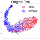
(a)

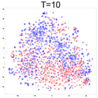
(b)

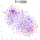
(c)

Fig. 1: PCA followed by a T-SNE projection of BERT embeddings of the sentences of DIAL corpus after T=0,10,1000 iterations of our framework (based on Sinkhorn divergence). Colors display the sensitive (i.e., binary gender) attribute.

Learning disentangled representations has received a growing interest as it has been shown to be useful for a wide variety of tasks (e.g., style transfer Fu et al. (2017), few shot learning Karn et al. (2021), fair classification Colombo et al. (2021d)). For text, the dominant approaches to learn such representations can be divided into two classes. The first one, relies on an adversary that is trained to recover the discrete sensitive attribute from the latent representation of the input Xie et al. (2017). However, as pointed out by Barrett et al. (2019), even though the adversary seems to do a perfect job during training, a fair amount of the sensitive information can be recovered from the latent representation when training a new adversary from scratch. The second line of research involves a regularizer that is a trainable surrogate of the mutual information (MI) (e.g., CLUB Cheng et al. (2020a), MIReny Colombo et al. (2021d), KNIFE Pichler et al. (2020), MINE Belghazi et al. (2018); Colombo et al. (2021b)) and achieves higher degrees of disentanglement. However, as highlighted by recent works McAllester and Stratos (2020); Song and Ermon (2019), these estimators are hard to use in practice and the optimization procedure (see App. D.4) involves several updates of the regularizer parameters at each update of the representation model. As a consequence, these procedures are both time consuming and involve extra hyperparameters (e.g., optimizer learning rates, architecture, number of updates of the nested loop) that need to be carefully selected which is often not such an easy task.

Contributions. In this work, we focus our attention on learning to disentangle textual representations from a discrete attribute. Our method relies on a novel family of regularizers based on discrepancy measures. We evaluate both the disentanglement and representation quality on fair text classification. Formally, our contribution is two-fold:
(1) A novel formulation of the problem of learning disentangled representations. Different from previous works–either minimizing a surrogate of MI or training an adversary–we propose to minimize a statistical measure of similarity between the underlying probability distributions conditioned to the sensitive attributes. This novel formulation allows us to derive new regularizers with convenient properties: (i) not requiring additional learnable parameters; (ii) alleviating computation burden; and (iii) simplifying the optimization dynamic.
(2) Applications and numerical results. We carefully evaluate our new framework on four different settings coming from two different datasets. We strengthen the experimental protocol of previous works Colombo et al. (2021d); Ravfogel et al. (2020) and test our approach both on randomly initialized encoder (using RNN-based encoder) and during fine-tuning of deep contextualized pretrained representations. Our experiments are conducted on four different main/sensitive attribute pairs and involve the training of over $280$ deep neural networks. Our findings show that: (i) disentanglement methods behave differently when applied to randomly initialized or to deep contextualized pretrained encoder; and (ii) our framework offers a better accuracy/disentanglement trade-off than existing methods (i.e., relying on an adversary or on a MI estimator) while being faster and easier to train. Model, data and code are available at https://github.com/PierreColombo/TORNADO.

2 Related Work

Considering a tuple $(X,S)$ where $X$ is a random variable (r.v.) defined on the space of text $\mathcal{X}$ and $S$ is a binary r.v. which corresponds to a sensitive attribute. Learning disentangled representations aims at learning the parameter $\theta$ of the encoder $f_{\theta}:\mathcal{X}\rightarrow\mathcal{Z}\subset\mathbb{R}^{d}$ which maps $X$ to a latent representation $Z=f_{\theta}(X)\in\mathbb{R}^{d}$, where $d\in\mathbb{N}_{*}$ corresponds to the dimension of the embedding space. The goal is that $Z$ retains as much useful information from $X$ while being oblivious of $S$. Among the numerous possible applications for disentangled representations, we choose to focus on fair classification as it is a natural task to define the aforementioned useful information. In the fair classification task, we assume access to $Y$, a binary r.v., which corresponds to the main label/attribute. In order to learn disentangled representations for fair classification, we follow previous works Beutel et al. (2017); Cheng et al. (2020b) and we will be minimizing the loss $\mathcal{L}(\phi,\psi,\theta)$, which is defined as follows:

$$\underbrace{\textrm{CE}\big{(}C_{\phi}(f_{\theta}(X)),Y\big{)}}_{\textrm{target task}}+\lambda\cdot\underbrace{R\big{(}f_{\theta}(X),S;\psi\big{)}}_{\textrm{regularizer}},$$ (1)

where $C_{\phi}:\mathcal{Z}\rightarrow\mathcal{Y}$ refers to the main classifier; $\phi$ to its learnable parameters; CE to the cross-entropy loss; R denotes the disentanglement regularizer; $\psi$ its parameters and $\lambda$ controls the trade-off between disentanglement and success in the classification task. We next review the two main methods that currently exist for learning textual disentangled representations: adversarial-based and MI-based.

2.1 Adversarial-Based Regularizers

In the context of disentangled representation learning, a popular method is to rely on adding an adversary to the encoder (e.g., texts Coavoux et al. (2018), images Xie et al. (2017), categorical data Beutel et al. (2017)). This adversary is competing against the encoder trying to learn the main task objective. In this line of work, $R(f_{\theta}(X),S;\psi)=-\textrm{CE}(C_{\psi}(f_{\theta}(X)),S)$ where $C_{\psi}:\mathcal{Z}\rightarrow\mathcal{S}$ refers to the adversarial classifier that is trained to minimize $\textrm{CE}(C_{\psi}(f_{\theta}(X)),S)$. Denoting by $\mathbb{P}_{Z|S=0}$ and $\mathbb{P}_{Z|S=1}$ the probability distribution of the conditional r.v. $Z|S=0$ and $Z|S=1$, respectively, these works build on the fact that if $\mathbb{P}_{Z|S=0}$ and $\mathbb{P}_{Z|S=1}$ are different, the optimal adversary will be able to recover sensitive information from the latent code $Z$. Although adversaries have achieved impressive results in many applications when applied to attribute removal, still a fair amount of information may remain in the latent representation Lample et al. (2018).

2.2 MI-Based Regularizers

To better protect sensitive information, the second class of methods involves direct mutual information minimization. MI lies at the heart of information theory and measures statistical dependencies between two random variables $Z$ and $S$ and find many applications in machine learning Boudiaf et al. (2020b, a, 2021). The MI is a non-negative quantity that is 0 if and only if $Z$ and $S$ are independent and is defined as follows:

$$I(Z;S) =\text{KL}(\mathbb{P}_{ZS}\|\mathbb{P}_{Z}\otimes\mathbb{P}_{S}),$$ (2)

where the joint probability distribution of $(Z,S)$ is denoted by $\mathbb{P}_{ZS}$; marginals of $Z$ and $S$ are denoted by $\mathbb{P}_{Z}$ and $\mathbb{P}_{S}$ respectively; and KL stands for the Kullback-Leibler divergence. Although computing the MI is challenging Paninski (2003); Pichler et al. (2022), a plethora of recent works devise new lower Belghazi et al. (2018); Oord et al. (2018) and upper bounds Cheng et al. (2020a); Colombo et al. (2021d) ${\tilde{I}_{\psi}(f_{\theta}(X);S)}$ where $\psi$ denotes the trainable parameters of the surrogate of the MI. In that case, $R(f_{\theta}(X),S;\psi)={\tilde{I}_{\psi}(f_{\theta}(X);S)}$. These methods build on the observation that if $I(Z;X)>0$ then $\mathbb{P}_{Z|S=0}$ and $\mathbb{P}_{Z|S=1}$ are different and information about the sensitive label $S$ remains in $Z$. Interestingly, these approaches achieve better results than adversarial training on various NLP tasks Cheng et al. (2020b) but involve the use of additional (auxiliary) neural networks.

2.3 Limitations of Existing Methods

The aforementioned methods involve the use of extra parameters (i.e., $\psi$) in the regularizer. As the regularizer computes a quantity based on the representation given by the encoder with parameter $\theta$, any modification of $\theta$ requires an adaptation of the parameter of $R$ (i.e., $\psi$). In practice, this adaptation is performed using gradient descent-based algorithms and requires several gradient updates. Thus, a nested loop (see App. D.4) is needed. Additional optimization parameters and the nested loop both induce additional complexity and require a fine-tuning which makes these procedures hard to be used on large-scale datasets. To alleviate these issues, the next section describes a parameter-free framework to get rid of the $\psi$ parameter present in $R$.

3 Proposed Method

This section describes our approach to learn disentangled representations. We first introduce the main idea and provide an algorithm to implement the general loss. We next describe the four similarity measures proposed in this approach.

3.1 Method Overview

As detailed in Section 2, existent methods generally rely on the use of neural networks either in the form of an adversarial regularizer or to compute upper/lower bounds of the MI between the embedding $Z=f_{\theta}(X)$ and the sensitive attribute $S$. Motivated by reducing the computational and complexity load, we aim at providing regularizers that are light and easy to tune. To this end, we need to get rid of the nested optimization loop, which is both time consuming and hard to tune in practice since the regularizer contains a large number of parameters (e.g., neural networks) that need to be trained by gradient descent. Contrarily to previous works in the literature, and following the intuitive idea that $\mathbb{P}_{Z|S=0}$ and $\mathbb{P}_{Z|S=1}$ should be as close as possible, we introduce similarity measures between $\mathbb{P}_{Z|S=0}$ and $\mathbb{P}_{Z|S=1}$ to build a regularizer $R$. It is worth noting that the similarity measures do not require any additional learnable parameters. For the sake of clarity, in the reminder of the paper we define $\mathbb{P}_{i}\triangleq\mathbb{P}_{Z|S=i}$ and $Z_{i}\triangleq f_{\theta}(X|S=i)$ for $i\in\{0,1\}$. Given a similarity measure defined as $\text{SM}:\mathcal{M}_{+}^{1}(\mathcal{Z})\times\mathcal{M}_{+}^{1}(\mathcal{Z})\longrightarrow\mathbb{R}_{+}$ where $\mathcal{M}_{+}^{1}(\mathcal{Z})$ denotes the space of probability distributions on $\mathcal{Z}$, we propose to regularize the downstream task by $\text{SM}(\mathbb{P}_{0},\mathbb{P}_{1})$. Precisely, the optimization problem boils down to the following objective:

$$\mathcal{L}(\phi,\theta)=\underbrace{\textrm{CE}(C_{\phi}(f_{\theta}(X)),Y)}_{\textrm{target task}}+\lambda\cdot\underbrace{\text{SM}(\mathbb{P}_{0},\mathbb{P}_{1})}_{\textrm{regularizer}}.$$ (3)

The proposed statistical measures of similarity, detailed in Section 3.2, have explicit and simple formulas. It follows that the use of neural networks is no longer necessary in the regularizer term which reduces drastically the complexity of the resulting learning problem. The disentanglement can be controlled by selecting appropriately the measure SM. For the sake of place, the algorithm we propose to solve (3) is deferred to the App. B.

3.2 Measure of Similarity between Distributions

In this work, we choose to focus on four different (dis-) similarity functions ranging from the most popular in machine learning such as the Maximum Mean Discrepancy measure (MMD) and the Sinkhorn divergence (SD) to standard statistical discrepancies such as the Jeffrey divergence (J) and the Fisher-Rao distance (FR).

3.2.1 Maximum Mean Discrepancy.

Let $k:\mathcal{Z}\times\mathcal{Z}\rightarrow\mathbb{R}$ be a kernel and $\mathcal{H}$ its corresponding Reproducing Kernel Hilbert Space with inner product $\langle.,.\rangle_{\mathcal{H}}$ and norm $\|.\|_{\mathcal{H}}$. Denote by $\mathcal{B}_{\mathcal{H}}=\{f\;|\;\|f\|_{\mathcal{H}}\leq 1\}$ the unit ball of $\mathcal{H}$. The Maximum Mean Discrepancy (MMD) Gretton et al. (2007) between the two conditional distributions $\mathbb{P}_{0},\mathbb{P}_{1}\in\mathcal{M}^{1}_{+}(\mathcal{Z})$ associated with the kernel $k$, is defined as:

$$\text{MMD}(\mathbb{P}_{0},\mathbb{P}_{1}) =\underset{\Psi\in\mathcal{B}_{\mathcal{H}}}{\sup}\big{\lvert}\mathbb{E}_{\mathbb{P}_{0}}[\Psi(Z_{0})]-\mathbb{E}_{\mathbb{P}_{1}}[\Psi(Z_{1})]\big{\rvert}$$

$$=\mathbb{E}_{\mathbb{P}_{0}\otimes\mathbb{P}_{0}}[k(Z_{0},Z_{0}^{\prime})]$$

$$\quad+\mathbb{E}_{\mathbb{P}_{1}\otimes\mathbb{P}_{1}}[k(Z_{1},Z_{1}^{\prime})]$$

$$\quad-2\,\mathbb{E}_{\mathbb{P}_{0}\otimes\mathbb{P}_{1}}[k(Z_{0},Z_{1})].$$

The MMD can be estimated with a quadratic computational complexity $\mathcal{O}(n^{2})$ where $n$ is the sample size. In this paper, MMD is computed using the Gaussian kernel $k:(z_{0},z_{1})\mapsto\exp(-\|z_{0}-z_{1}\|^{2}/2\sigma^{2})$, where $\|\cdot\|$ is the usual euclidean norm.

3.2.2 Sinkhorn Divergence.

The Wasserstein distance aims at comparing two probability distributions through the resolution of the Monge-Kantorovich mass transportation problem (see e.g.  Villani (2003); Peyré and Cuturi (2019)):

$$\text{W}^{p}(\mathbb{P}_{0},\mathbb{P}_{1})=\underset{\pi~{}\in~{}\mathcal{U}(\mathbb{P}_{0},\mathbb{P}_{1})}{\min}\int_{\mathcal{Z}\times\mathcal{Z}}\|z_{0}-z_{1}\|^{p}d\pi(z_{0},z_{1}),$$ (4)

where $\mathcal{U}(\mathbb{P}_{0},\mathbb{P}_{1})=\{\pi\in\mathcal{M}^{1}_{+}(\mathcal{Z}\times\mathcal{Z}):\;\;\int\pi(z_{0},z_{1})dy=\mathbb{P}_{0}(z_{0});\int\pi(z_{0},z_{1})dx=\mathbb{P}_{1}(z_{1})\}$ is the set of joint probability distributions with marginals $\mathbb{P}_{0}$ and $\mathbb{P}_{1}$. For the sake of clarity, the power $p$ in W^p is omitted in the remainder of the paper. When $\mathbb{P}_{0}$ and $\mathbb{P}_{1}$ are discrete measures, (4) is a linear problem and can be solved with a supercubic complexity $\mathcal{O}(n^{3}\log(n))$, where $n$ denotes the sample size. To overcome this computational drawback, Cuturi et al. (2013) added an entropic regularization term to the transport cost to obtain a strongly convex problem solvable using the Sinkhorn-Knopp algorithm Sinkhorn (1964) leading to a computational cost of $\mathcal{O}(n^{2})$. The bias introduced by the regularization term, i.e., the quantity is not longer zero when comparing to the same probability distribution, have been corrected by Genevay et al. (2019) leading to the known Sinkhorn Divergence (SD) defined as:

$$\text{{SD}}_{\varepsilon}(\mathbb{P}_{0},\mathbb{P}_{1})=\text{W}_{\varepsilon}(\mathbb{P}_{0},\mathbb{P}_{1})-\frac{1}{2}\sum_{i=0}^{1}\text{W}_{\varepsilon}(\mathbb{P}_{i},\mathbb{P}_{i}),$$

where $\text{W}_{\varepsilon}(\mathbb{P}_{0},\mathbb{P}_{1})$ is equal to

$$\underset{\pi~{}\in~{}\mathcal{U}(\mathbb{P}_{0},\mathbb{P}_{1})}{\min}\int_{\mathcal{Z}\times\mathcal{Z}}\|z_{0}-z_{1}\|^{p}d\pi(z_{0},z_{1})+\varepsilon\,\text{H}(\pi),$$

with $\text{H}(\pi)=\int\pi(z_{0},z_{1})\log(\pi(z_{0},z_{1}))dz_{0}dz_{1}$.

3.2.3 Fisher-Rao Distance.

The Fisher-Rao distance (FR) (Rao, 1945) is a Riemannian metric defined on the space of parametric distributions relying on the Fisher information. The Fisher information matrix provides a natural Riemannian structure Amari (2012). It is known to be more accurate than popular divergence measures Costa et al. (2015). Let $\mathcal{M}_{+}^{1}(\mathcal{Z},\mathcal{P})$ be the family of parametric distributions with the parameter space $\mathcal{P}\subset\mathbb{R}^{d}$. The FR distance is defined as the geodesic distance between elements (i.e., probability measures) on the manifold $\mathcal{M}_{+}^{1}(\mathcal{Z},\mathcal{P})$. Parametrizing $\mathbb{P}_{0},\mathbb{P}_{1}$ by parameters $p_{1},p_{2}\in\mathcal{P}$, respectively, such that $\mathbb{P}^{p_{0}}_{0}\triangleq\mathbb{P}_{0}$ and $\mathbb{P}^{p_{1}}_{1}\triangleq\mathbb{P}_{1}$, the FR distance between $\mathbb{P}_{0}^{p_{0}}$ and $\mathbb{P}_{1}^{p_{1}}$ is defined as:

$$\text{FR}(\mathbb{P}_{0}^{p_{0}},\mathbb{P}_{1}^{p_{1}})=\min_{\gamma}\int|\sqrt{\gamma^{\prime}(t)^{\top}G(p_{0},p_{1})\gamma(t)}|dt$$ (5)

where $\gamma(t)$ is the curve connecting $p_{0}$ and $p_{1}$ in the parameter space $\mathcal{P}$; and $G(p_{0},p_{1})$ is the Fisher information matrix of $(p_{0},p_{1})$. In general, the optimization problem of (5) can be solved using the well-known Euler-Lagrange differential equations leading to computational difficulties. Atkinson and Mitchell (1981) have provided computable closed-form for specific families of distributions such as Multivariate Gaussian with diagonal covariance matrix. Under this assumption, the parameters $p_{0}$ and $p_{1}$ are defined by $p_{i,j}=(\mu_{i,j},\sigma_{i,j})\in\mathbb{R}^{2}$ for $i\in\{0,1\}$ and $1\leq j\leq d$ with $\mu_{i}\in\mathbb{R}^{d}$ the mean vector and $\text{Diag}(\sigma_{i})$ the diagonal covariance matrix of $\mathbb{P}_{i}$ where $\sigma_{i}$ is the variance vector. The resulting FR metric admits the following closed-form (see e.g. Pinele et al. (2020):

$$\text{FR}(\mathbb{P}_{0}^{p_{0}},\mathbb{P}_{1}^{p_{1}})=\sqrt{\sum_{j=1}^{d}\left[d_{\text{FR}}(p_{0,j},p_{1,j})\right]^{2}},$$

where $d_{\text{FR}}(p_{0,j},p_{1,j})$ is the univariate Fisher-Rao detailed in the App. A.1 for the sake of space.

3.2.4 Jeffrey Divergence.

The Jeffrey divergence (J) is a symmetric version of the Kullback-Leibler (KL) divergence and measures the similarity between two probability distributions. Formally, it is defined as follow:

$$\text{J}(\mathbb{P}_{0},\mathbb{P}_{1})=\frac{1}{2} \big{[}\text{KL}(\mathbb{P}_{0}\|\mathbb{P}_{1})+\text{KL}(\mathbb{P}_{1}\|\mathbb{P}_{0})\big{]}.$$

Computing the $\text{KL}(\mathbb{P}_{0}\|\mathbb{P}_{1})$ either requires to have knowledge of $\mathbb{P}_{0}$ and $\mathbb{P}_{1}$, or to have knowledge about the density ratio Rubenstein et al. (2019). Without any further assumption on $\mathbb{P}_{0}$, $\mathbb{P}_{1}$ or the density ratio, the resulting inference problem is known to be provably hard Nguyen et al. (2010). Although previous works have addressed the estimation problem without making assumptions on $\mathbb{P}_{0}$ and $\mathbb{P}_{1}$ Oord et al. (2018); Hjelm et al. (2018); Belghazi et al. (2018), these methods often involve additional parameters (e.g., neural networks Song and Ermon (2019), kernels McAllester and Stratos (2020)), require additional tuning Hershey and Olsen (2007), and are time expensive. Motivated by speed, simplicity and to allow for fair comparison with FR, for this specific divergence, we choose to make the assumption that $\mathbb{P}_{0}$ and $\mathbb{P}_{1}$ are multivariate Gaussian distributions with mean vector $\mu_{0}$ and $\mu_{1}$ and diagonal covariance matrices: $\Sigma_{0}$ and $\Sigma_{1}$. Thus, $\text{KL}(\mathbb{P}_{0},\mathbb{P}_{1})$ boils down to:

$$\log\frac{|\Sigma_{0}|}{|\Sigma_{1}|}-d+\text{Tr}(\Sigma_{0}^{-1}\Sigma_{1})+(\mu_{0}-\mu_{1})^{T}\Sigma_{0}^{-1}(\mu_{0}-\mu_{1}),$$

where $\text{Tr}(\Sigma_{0}^{-1}\Sigma_{1})$ is the trace of $\Sigma_{0}^{-1}\Sigma_{1}$.

Remark.

FR and J are computed under the multivariate Gaussian with diagonal covariance matrix assumption. In this case, the Sinkhorn approximation is not needed as (4) can be efficiently computed thanks to the following closed-form:

$$\mathrm{W}(\mathbb{P}_{0},\mathbb{P}_{1})=\|\mu_{0}-\mu_{1}\|^{2}+\mathrm{Tr}\left(\Sigma_{0}+\Sigma_{1}-2(\Sigma_{0}\Sigma_{1})^{1/2}\right)$$

Remark.

Quantities defined in this section are replaced by their empirical estimate. Due to space constraints, the formula are described in App. A.2.

4 Experimental Setting

In this section, we describe the datasets, metrics, encoder and baseline choices. Additional experimental details can be found in App. D. For fair comparison, all models were re-implemented.

4.1 Datasets

To ensure backward comparison with previous works, we choose to rely on the DIAL Blodgett et al. (2016) and the PAN Rangel et al. (2014) datasets. For both, main task labels ($Y$) and sensitive labels ($S$) are binary, balanced and splits follow Barrett et al. (2019). Random guessing is expected to achieve near 50% of accuracy.
The DIAL corpus has been automatically built from tweets and the main task is either polarity or mention prediction. The sensitive attribute is related to race (i.e., non-Hispanic blacks and non-Hispanic whites) which is obtained using the author geo-location and the words used in the tweet.
The PAN corpus is also composed of tweets and the main task is to predict a mention label. The sensitive attribute is obtained through a manual process and annotations contain the age and gender information from 436 Twitter users.

4.2 Metrics

For the choice of the evaluation metrics, we follow the experimental setting of Colombo et al. (2021d); Elazar and Goldberg (2018); Coavoux et al. (2018). To measure the success of the main task, we report the classification accuracy. To measure the degree of disentanglement of the latent representation we train from scratch an adversary to predict the sensitive labels from the latent representation. In this framework, a perfect model would achieve a high main task accuracy (i.e., near 100%) and a low (i.e., near 50%) accuracy as given by the adversary prediction on the sensitive labels. Following Colombo et al. (2021d), we also report the disentanglement dynamic following variations of $\lambda$ and train a different model for each $\lambda\in[0.001,0.01,0.1,1,10]$.

4.3 Models

Choice of the encoder. Previous works that aim at learning disentangled representations either focus on randomly initialized RNN-encoders Colombo et al. (2021d); Elazar and Goldberg (2018); Coavoux et al. (2018) or only use pretrained representations as a feature extractor Ravfogel et al. (2020). In this work, we choose to fine-tune BERT during training as we believe it to be a more realistic setting.
Choice of the baseline models. We choose to compare our methods against adversarial training from Elazar and Goldberg (2018); Coavoux et al. (2018) (model named ADV) and the recently MI bound introduced in Colombo et al. (2021d) (named MI) which has been shown to be more controllable than previous MI-based estimators.

5 Numerical Results

In this section, we gather experimental results for fair classification task. We study our framework when working either with RNN or BERT encoders. The parameter $\lambda$ (see (3)) controls the trade-off between success on the main task and disentanglement for all models.

5.1 Overall Results

		RNN			BERT
Dat.	Loss	$\lambda$	$Y$($\uparrow$)	$S$($\downarrow$)	$\lambda$	$Y$($\uparrow$)	$S$($\downarrow$)
Sent.	CE	0.0	73.2	68.7	0.0	76.2	76.7
	ADV	1.0	71.9	56.1	0.1	74.9	72.3
	MI	0.1	71.6	56.3	0.1	74.5	70.3
	W	10	69.3	50.0	0.01	72.3	54.2
	J	10	70.0	54.1	10	56.7	56.7
	FR	10	57.6	52.0	10	57.4	57.4
	MMD	10	70.3	55.7	0.1	71.0	56.2
	SD	10	70.4	56.5	0.1	73.8	54.3
Ment.	CE	0.0	77.5	66.1	0.0	81.7	79.1
	ADV	0.1	77.0	55.4	0.1	82.2	75.3
	MI	10	70.0	55.7	10	74.9	55.0
	W	10	77.6	50.0	0.01	79.0	53.0
	J	10	73.4	53.3	1	53.5	56.9
	FR	10	75.6	53.6	1	60.0	60.0
	MMD	10	77.8	58.0	0.1	80.0	52.4
	SD	10	77.8	56.8	0.1	78.4	52.3

Tab. 1: Results on the fair classification task: the main task (higher is better) accuracy corresponds to the column with $Y(\uparrow)$ and $S(\downarrow)$ denotes the sensitive task accuracy (lower is better). CE refers to a classifier trained with CE loss solely ($\lambda=0$ in (1)).

General observations. Learning disentangled representations is made more challenging when $S$ and $Y$ are tightly entangled. By comparing Fig. 2 and Fig. 3, we notice that the race label (main task) is easier to disentangled from the sentiment compared to the mention.
Randomly initialized RNN encoders. To allow a fair comparison with previous works, we start by testing our framework with RNN encoders on the DIAL dataset. Results are depicted in Fig. 2. It is worth mentioning that we are able to observe a similar phenomenon that the one reported in Colombo et al. (2021d). More specifically, we observe: (i) the adversary degenerates for $\lambda=10$ and does not allow to reach perfectly disentangled representations nor to control the desirable degree of disentanglement; (ii) the MI allows better control over the desirable degree of disentanglement and achieves better-disentangled representations at a reduced cost on the main task accuracy. Fig. 2 shows that the encoder trained using the statistical measures of similarity–both with and without the multivariate Gaussian assumption–are able to learn disentangled representations. We can also remark that our losses follow an expected behaviour: when $\lambda$ increases, more weight is given to the regularizer, the sensitive task accuracy decreases, thus the representations are more disentangled according to the probing-classifier. Overall, we observe that the W regularizer is the best performer with optimal performance for $\lambda=1$ on both attributes. On the other hand, we observe that FR and J divergence are useful to learn to disentangle the representations but disentangling using these similarity measures comes with a greater cost as compared to W. Both MMD and SD also perform well and are able to learn disentangled representations with little cost on the main task performance. However, on DIAL, they are not able to learn perfectly disentangled representations. Similar conclusions can be drawn on PAN and results are reported in App.  C.1.

BERT encoder. Results of the experiment conducted with BERT encoder are reported in Fig. 3. As expected, we notice that on both tasks the main and the sensitive task accuracy for small values of $\lambda$ is higher than when working with RNN encoders. When training a classifier without disentanglement constraints (i.e., case $\lambda=0$ in (1)), which corresponds to the dash lines in Fig. 2 and Fig. 3, we observe that BERT encoder naturally preserves more sensitive information (i.e., measured by the accuracy of the adversary) than randomly initialized encoder. Contrarily to what is usually undertaken in previous works (e.g., Ravfogel et al. (2020)), we allow the gradient to flow in BERT encoder while preforming fine-tuning. We observe a different behavior when compared to previous experiments. Our losses under the Multivariate diagonal Gaussian assumption (i.e., W, J, FR ) can only disentangle the representations at a high cost on the main task (i.e., perfect disentanglement corresponds to performance on the main task close to a random classifier). When training the encoder with either SD or MMD, we are able to learn disentangled representations with a limited cost on the main task accuracy: $\lambda=0.1$ achieves good disentanglement with less than 3% of loss in the main task accuracy. The methods allow little control over the degree of disentanglement and there is a steep transition between light protection with no loss on the main task accuracy and strong protection with discriminative features destruction.

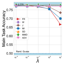
(a)

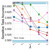
(b)

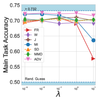
(c)

(d)

Fig. 2: Results on DIAL with RNN. Dash lines correspond to model trained with CE loss solely (i.e., case $\lambda=0$ in (1)). Figures on the left are dedicated to the mention attribute while the one on the rights reports results on the Sentiment attribute. The main task consists in predicting $Y$ thus higher is better. The sensitive task accuracy is obtained by training a classifier to $S$ on the final representation thus an ideal model would reach $50\%$ of accuracy.

Takeaways. Our new framework relying on statistical Measures of Similarity introduces powerful methods to learn disentangled representations. When working with randomly initialized RNN encoders to learn disentangled representation, we advise relying on W. Whereas in presence of pretrained encoders (i.e., BERT), we observe a very different behavior  and recommend using SD.

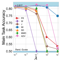
(a)

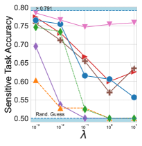
(b)

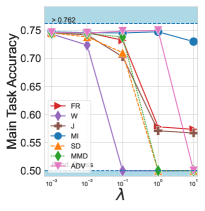
(c)

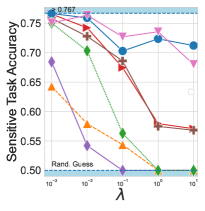
(d)

Fig. 3: Results on DIAL for mention (left) and sentiment (right) attribute using a pretrained BERT.

(a)

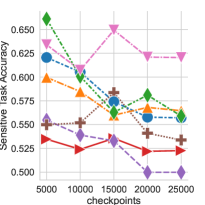
(b)

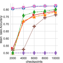
(c)

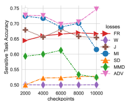
(d)

Fig. 4: Training Dynamic on DIAL for the mention label with using RNN (left $\lambda=10$ ) and BERT (right $\lambda=0.1$) encoders.

	Method	# params.	1 upd.	1 epoch.
RNN	ADV	2220 $-0.6\%$	0.11	551 $-17\%$
	MI	2234	0.13	663
	FR	2206 $-1.3\%$	0.10	508 $-23\%$
	W		0.10	509 $-23\%$
	J		0.10	507 $-23\%$
	MMD		0.10	520 $-22\%$
	SD		0.10	544 $-18\%$
	Method	# params.	1 upd.	1 epoch.
BERT	ADV	109576 $-0.01\%$	0.48	2424 $-10\%$
	MI	109591	0.55	2689
	FR	109576 $-0.03\%$	0.47	2290 $-14\%$
	W		0.47	2290 $-14\%$
	J		0.47	2307 $-14\%$
	MMD		0.48	2323 $-14\%$
	SD		0.48	2347 $-13\%$

Tab. 2: Speed and number of model parameters (given in thousand) when working with DIAL. The runtime for 1 gradient update (denoted 1 upd.) or for 1 epoch is given for a batch of 64 when running our models on a single NVIDIA-V100. The relative improvements (in %) are given with respect to the MI model, which is our strongest baseline.

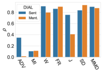
(a)

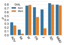
(b)

Fig. 5: Absolute Pearson correlation between the values of $R$ and the sensitive task accuracy.

5.2 Speed Gain and Parameter Reduction

We report in Table 2 the training time and the number of parameters of each method. The reduced number of parameters brought by our method is marginal, however getting rid of these parameters is crucial. Indeed, they require a nested loop and require a fined selection of the hyperparameters which complexify the global system dynamic.
Takeaways. Contrarily to MI or Adversarial based regularizer that are difficult (or even prohibitive) to be implemented on large-scale datasets, our framework is simpler and consistently faster which makes it a better candidate when working with large-scale datasets.

6 Further Analysis

Results presented in Section 5.1 have shown a different behaviour for RNN and BERT based encoders and, for different measures of similarity. Here, we aim at understanding of this phenomena.

6.1 Training Dynamic

In the previous section, we examine the change of the measures during the training.
Takeaways. When using a RNN encoder, the system is able to maximize the main task accuracy while jointly minimizing most of the similarity measures. For BERT where the model is more complex, for measures relying on the diagonal gaussian multivariate assumption either the disentanglement plateau (e.g., FR or J) or the system fails to learn discriminative features and perform poorly on the main task (e.g., W). When combined with BERT both SD and MMD can achieve high main task accuracy while protecting the sensitive attribute.

6.2 Correlation Analysis

In this experiment, we investigate how predictive of the disentanglement is each similarity measure, i.e., does a lower value of similarity measure indicates better disentangled representations? We gather for both the mention and sentiment attribute 5 checkpoints per model (i.e., each regularizer and each value of $\lambda$ corresponds to one model). For each RNN model, we select one checkpoint after $5\mathrm{k},10\mathrm{k},15\mathrm{k},20\mathrm{k},25\mathrm{k}$ gradient updates, and for BERT we select one checkpoint after $2\mathrm{k},4\mathrm{k},6\mathrm{k},8\mathrm{k},10\mathrm{k}$ gradient updates to obtain the same number of models. For each type of loss, we ended with 50 models. For each model and each checkpoint, we train an adversary, compute the sensitive task accuracy and evaluate the Pearson correlation between the sensitive task accuracy and the corresponding similarity measure. Results are presented in Fig. 5.

Takeaways. Both ADV and MI poorly are correlated with the degree of disentanglement of the learned representations. We find this result not surprising at light of the findings of Xie et al. (2017) and Song and Ermon (2019). All our losses achieve high correlation ($\rho\geq 78$) except for J in the mention task with both encoders, and the FR with BERT on the mention task that achieves medium/low correlation. We believe, that the high correlation showcases the validity of the proposed approaches.

7 Summary and Concluding Remarks

We have introduced a new framework for learning disentangled representations which is faster to train, easier to tune and achieves better results than adversarial or MI-based methods. Our experiments on the fair classification task show that for RNN encoders, our methods relying on the closed-form of similarity measures under a multivariate Gaussian assumption can achieve perfectly disentangled representations with little cost on the main tasks (e.g. using Wasserstein). On BERT representations, our experiments show that the Sinkhorn divergence should be preferred. It can achieves almost perfect disentanglement at little cost but allows for fewer control over the degree of disentanglement.

Appendix A Additional details on Statistical Measures of Similarity

It is the purpose of this part to recall additional details on similarity measures defined in the core paper.

A.1 Univariate Fisher-Rao distance

Here, we recall the definition of the univariate Fisher-Rao distance used in the Section 3.2. Let $\mathbb{Q}_{1},\mathbb{Q}_{2}$ be two univariate probability distributions with mean $m_{1},m_{2}\in\mathbb{R}$ and standard deviation $\sigma_{1},\sigma_{2}\in\mathbb{R}$. Thus, the univariate Fisher-Rao distance between the tuples $(m_{1},\sigma_{1})$ and $(m_{2},\sigma_{2})$ denoted by $d_{\text{FR}}$ is defined as:

$$\sqrt{2}\log\frac{\sqrt{\frac{(m_{1}-m_{2})^{2}}{2}+(\sigma_{1}+\sigma_{2})^{2}}+\sqrt{\frac{(m_{1}-m_{2})^{2}}{2}+(\sigma_{1}-\sigma_{2})^{2}}}{\sqrt{\frac{(m_{1}-m_{2})^{2}}{2}+(\sigma_{1}+\sigma_{2})^{2}}-\sqrt{\frac{(m_{1}-m_{2})^{2}}{2}+(\sigma_{1}-\sigma_{2})^{2}}}.$$

A.2 Empirical versions of Statistical Measures of Similarity

Our experimental setting involves the tuple $\left(X^{i},S^{i},Y^{i}\right)_{i=1}^{n}$ where $X^{1},\ldots,X^{n}$ is a sample of texts drawn from the random variable $X\in\mathcal{X}$, $S^{1},\ldots,S^{n}$ is a sample of binary random variables corresponding to the sensitive attribute and $Y^{1},\ldots,Y^{n}$ is a sample of binary random variables coming from the classification task. Considering the embedding function $f_{\theta}$, we denote by $Z^{1},\ldots,Z^{n}$ the embedding sample such that $Z^{i}=f_{\theta}(X^{i})$ for every $1\leq i\leq n$. Assume that $\{i_{1},\ldots,i_{n_{0}}\}$ and $\{j_{1},\ldots,i_{n_{1}}\}$ are two subsets of $\{1,\ldots,n\}$ such that $S_{i_{k}}=0$ and $S_{j_{l}}=1$ for every $1\leq k\leq n_{0}$ and $1\leq l\leq n_{1}$. The empirical versions of the conditional measures $\mathbb{P}_{0},\mathbb{P}_{1}$ are given by

$$\hat{\mathbb{P}}_{0}=\frac{1}{n_{0}}\sum_{i\in\{i_{1},\ldots,i_{n_{0}}\}}\delta_{Z^{i}},\;\hat{\mathbb{P}}_{1}=\frac{1}{n_{1}}\sum_{j\in\{j_{1},\ldots,j_{n_{1}}\}}\delta_{Z^{j}}.$$

In practice, distances recalled in Section  3.2 are computed between $\hat{\mathbb{P}}_{0}$ and $\hat{\mathbb{P}}_{1}$ leading to the following distances.

Maximum Mean Discrepancy. The MMD is defined as:

$$\text{MMD}(\hat{\mathbb{P}}_{0},\hat{\mathbb{P}}_{1}) =\frac{1}{n_{0}(n_{0}-1)}\sum_{\begin{subarray}{c}i,k\in\{i_{1},\ldots,i_{n_{0}}\}\\ i\neq k\end{subarray}}k(Z^{i},Z^{k})$$

$$+\frac{1}{n_{1}(n_{1}-1)}\sum_{\begin{subarray}{c}j,l\in\{j_{1},\ldots,j_{n_{1}}\}\\ j\neq l\end{subarray}}k(Z^{j},Z^{l})$$

$$-\frac{2}{n_{0}n_{1}}\sum_{\begin{subarray}{c}i\in\{i_{1},\ldots,i_{n_{0}}\}\\ j\in\{j_{1},\ldots,j_{n_{1}}\}\end{subarray}}k(Z^{i},Z^{j}).$$

Sinkhorn divergence. Let $\mathbf{1}_{n_{0}},\mathbf{1}_{n_{1}}$ denote the vectors of one with size $n_{0},n_{1}$ respectively. Let $\mathcal{U}(\hat{\mathbb{P}}_{0},\hat{\mathbb{P}}_{1})=\{\Pi\in\mathbb{R}^{n_{0}\times n_{1}}\;|\;\;\Pi\mathbf{1}_{n_{1}}=\mathbf{1}_{n_{0}}/n_{0},\;\;\Pi^{\top}\mathbf{1}_{n_{0}}=\mathbf{1}_{n_{1}}/n_{1}\}$ be the set of joint probability distributions with marginals $\hat{\mathbb{P}}_{0}$ and $\hat{\mathbb{P}}_{1}$ where $/$ is the element-wise division. The Sinkhorn approximation of the 1-Wasserstein distance, denoted by $\text{W}_{\varepsilon}(\hat{\mathbb{P}}_{0},\hat{\mathbb{P}}_{1})$, is defined as the following optimization problem:

$$\underset{\Pi~{}\in~{}\mathcal{U}(\hat{\mathbb{P}}_{0},\hat{\mathbb{P}}_{1})}{\min}\sum_{\begin{subarray}{c}i\in\{i_{1},\ldots,i_{n_{0}}\}\\ j\in\{j_{1},\ldots,j_{n_{1}}\}\end{subarray}}\Pi_{i,j}\text{D}_{i,j}+\varepsilon\sum_{\begin{subarray}{c}i\in\{i_{1},\ldots,i_{n_{0}}\}\\ j\in\{j_{1},\ldots,j_{n_{1}}\}\end{subarray}}\Pi_{i,j}\log(\Pi_{i,j}),$$

where $\text{D}_{i,j}$ is the euclidean distance between $Z^{i}$ and $Z^{j}$. We limit ourselves to the 1-Wasserstein for the sake of place. The Sinkhorn divergence is then:

$$\text{{SD}}_{\varepsilon}(\hat{\mathbb{P}}_{0},\hat{\mathbb{P}}_{1})=\text{W}_{\varepsilon}(\hat{\mathbb{P}}_{0},\hat{\mathbb{P}}_{1})-\frac{1}{2}\sum_{i=0}^{1}\text{W}_{\varepsilon}(\hat{\mathbb{P}}_{i},\hat{\mathbb{P}}_{i}).$$

It is worth noticing that a robust version of the Wasserstein distance can be found in Staerman et al. (2021a) (see also Staerman et al. (2021c)).

Fisher-Rao distance. The Fisher-Rao distance is defined as

$$\text{FR}(\hat{\mathbb{P}}_{0}^{\hat{p}_{0}},\hat{\mathbb{P}}_{1}^{\hat{p}_{1}})=\sqrt{\sum_{j=1}^{d}\left[d_{\text{FR}}(\hat{p}_{0,j},\hat{p}_{1,j})\right]^{2}},$$

where $d_{\text{FR}}(\hat{p}_{0,j},\hat{p}_{1,j})$ is defined as in Section  A.1, and $m_{1},m_{2}$ and $\sigma_{1},\sigma_{2}$ are replaced by $\hat{\mu}_{0,j},\hat{\mu}_{1,j}$ and $\hat{\sigma}_{0,j},\hat{\sigma}_{1,j}$ the classical (univariate) unbiased mean and standard deviation estimators respectively.

Jeffrey divergence. Let $(\hat{\mu}_{0},\hat{\Sigma}_{0})$ and $(\hat{\mu}_{1},\hat{\Sigma}_{1})$ be the mean and the covariance matrix estimators of the samples $Z^{i_{1}},\ldots,Z^{i_{n_{0}}}$ and $Z^{j_{1}},\ldots,Z^{j_{n_{1}}}$ respectively. Jeffrey divergence–under the multivariate Gaussian assumption–boils down to:

$$\log\frac{|\hat{\Sigma}_{0}|}{|\hat{\Sigma}_{1}|}-d+\text{Tr}(\hat{\Sigma}_{0}^{-1}\hat{\Sigma}_{1})+(\hat{\mu}_{0}-\hat{\mu}_{1})^{T}\hat{\Sigma}_{0}^{-1}(\hat{\mu}_{0}-\hat{\mu}_{1}).$$

Furthermore, under the multivariate Gaussian assumption, the Wasserstein distance writes as follows:

$$\text{W}(\hat{\mathbb{P}}_{0},\hat{\mathbb{P}}_{1})=\|\hat{\mu}_{0}-\hat{\mu}_{1}\|^{2}+\mathrm{Tr}\left(\hat{\Sigma}_{0}+\hat{\Sigma}_{1}-2(\hat{\Sigma}_{0}\hat{\Sigma}_{1})^{1/2}\right)$$

Appendix B Algorithm

The algorithm we propose to compute (3) involves a simple training loop and is described in Algorithm  1.

Algorithm 1 Training Algorithm

1:Input $\mathcal{D}=\{(x_{j},s_{j},y_{j}),\forall j\in[1,n]\}$, $\theta$ weights of the encoder network, $\phi$ parameters of the main classifier.

2:Initialize parameters $\theta$, $\phi$.

3:while $(\theta,\phi)$ not converged do $\triangleright$ Single loop

4:     Sample a batch $\mathcal{B}$ from $\mathcal{D}$

5:     Compute CE $\triangleright$ Classification Loss

6:     Compute SM $\triangleright$ Disentanglement Loss

7:     Update $\theta,\phi$ with $\mathcal{B}$ using AdamW.

8:end while

9:Output Encoder and main classifier weights ${\theta,\phi}$

Appendix C Additional Results

In this section, we gather additional experimental results.

C.1 Results on PAN

		RNN			BERT
Dat.	Loss	$\lambda$	$Y$($\uparrow$)	$S$($\downarrow$)	$\lambda$	$Y$($\uparrow$)	$S$($\downarrow$)
Age	CE	0.0	85.7	60.0	0.0	87.0	65.0
	ADV	1	82.5	57.1	0.01	87.0	60.0
	MI	0.1	81.9	56.7	0.1	86.2	62.0
	W	10	82.9	50.0	0.01	84.3	52.1
	J	1	81.3	53.8	1	66.3	57.5
	FR	10	63.3	50.0	10	64.4	56.5
	MMD	10	83.3	50.1	0.1	85.2	54.4
	SD	10	80.0	50.0	0.1	80.2	52.4
Gender	CE	0.0	85.7	59.1	0.0	87.0	65.0
	ADV	0.1	77.0	55.4	0.01	87.3	61.3
	MI	10	70.0	55.7	0.1	86.8	63.9
	W	10	77.6	50.0	0.01	83.7	51.7
	J	10	73.4	53.3	1	62.7	54.3
	FR	1	75.6	53.6	1	62.1	58.1
	MMD	10	77.8	56.8	0.1	85.7	51.4
	SD	10	77.5	58.0	0.1	80.7	51.7

Tab. 3: Results on the fair classification task: the main task (higher is better) accuracy is correspond to the column with $Y(\uparrow)$ and $S\downarrow$ denotes the sensitive task accuracy respectively (lower is better). $\lambda$ (see Eq. 3 control the trade-off between success on the main task and disentanglement.

We report in Fig. 6 and Fig. 7 the results of the disentanglement analysis on the PAN dataset.
RNN encoders. We can make the same observations that the one done on DIAL in Section  5.1. We observe that the W regularizer performs well and is among the most controllable loss. It is worth noting the good performance of the SD and MMD losses which both work well on the RNN encoder.
BERT. For BERT encoder, we observe a similar steep transition than in Section  5.1 and we can draw similar conclusions. FR , W and J fail to disentangle BERT representation with little cost on the main task. SD and MMD achieve good results.
Takeaways. When working with randomly initialized RNN encoders to learn disentangled representation we advise relying on W and when working with pretrained encoder we advise to rely on the SD.

C.2 On the Diagonal Gaussian Assumption

Our closed-form for the Fisher-Rao metric relies on the diagonal Gaussian assumption that we have also made for W and J for a fair comparison. In this experiment (see Fig. 8), we examine this assumption by evaluating the relative distance (using a $L_{2}$-norm) between the empirical covariance matrix and a diagonal matrix.
Takeaways. Interestingly, as $\lambda$ increases, the empirical covariance matrix becomes closer to a diagonal matrix. For BERT, we observe that the W saturates and the distance for $\lambda>0.1$ is higher than for RNN. This might be the result of the optimization problems identified in Fig. 4. Hence, we observe that our methods–when learning more disentangled representations–is that the covariance matrix becomes closer to a diagonal matrix.

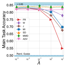
(a)

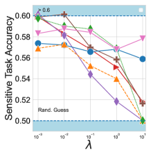
(b)

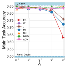
(c)

(d)

Fig. 6: Results on PAN with randomly initialized RNN encoders. Dash lines correspond to model trained with CE loss solely (i.e case $\lambda=0$ in (1)). Figures on the left are dedicated to the age attribute while the one on the rights reports results on the gender attribute. The main task consists in predicting $Y$ thus higher is better. The sensitive task accuracy is obtained by training a classifier to $S$ on the final representation thus an ideal model would reach 50% of accuracy

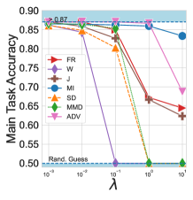
(a)

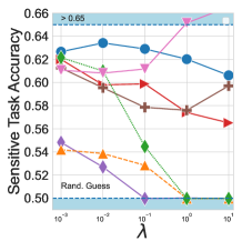
(b)

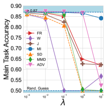
(c)

(d)

Fig. 7: Results on PAN for age (on the left) and gender (on the right) attribute using a pretrained BERT encoder.

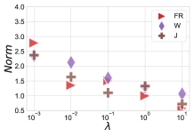
(a)

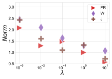
(b)

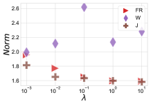
(c)

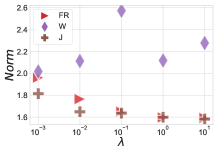
(d)

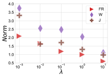
(e)

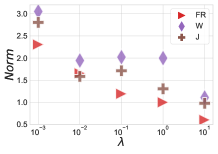
(f)

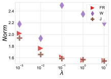
(g)

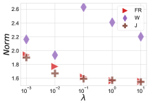
(h)

Fig. 8: Relative distance as measured by a $L_{2}$ norm between the empirical covariance matrix and a diagonal matrix on PAN dataset for various values of $S$.

Appendix D Experimental Details

D.1 Replication

In this section we gather the model details we used in our experiments. All models rely on the tokenizer based on Word Piece Schuster and Nakajima (2012) and is similar to the one used for BERT (i.e bert-base-uncased) and possess over $40k$ tokens.

Model Architecture for the RNN encoder.

For the randomly initialized RNN encoder, we use a bidirectionnal GRU Chung et al. (2014) that is composed of 2 layers with an hidden dimension of 128. For activation, we use LeakyReLU Xu et al. (2015) and the classification head is composed of fully connected layers of input dimension 256. The learning rate of AdamW Loshchilov and Hutter (2017) is set to $0.0001$ and the dropout Srivastava et al. (2014) is set to 0.2. The number of warmup steps Vaswani et al. (2017) is set to 1000.

Computational Resources.

For all 140 models, we train on NVIDIA-V100 with 32GB of RAM. Each model is trained for 30k steps and the model with the best disentanglement accuracy is selected based on the validation set. Each model takes around 5 hours to train. Evaluation requires to train and adversary composed of 3 hidden layers of input 128-128-128-2. The evaluation which involves the training of the probing classifier takes below 1 hour of GPU time. Overall, we train 6 different classifiers per model which correspond to 840 models.

Model Architecture for the BERT encoder.

For the BERT encoder, we add a classification head composed of one fully connected layer. We use a learning rate of $0.00001$ for AdamW and he number of warmup steps is set to 1000.

Computational Resources.

For all the 140 models, we train on NVIDIA-V100 with 32GB of RAM. Each model is trained for 10k steps, which correspond to the convergence of the model and the model with the best disentanglement accuracy is selected based on the validation set. Each model takes approximately 3 hours to train. Evaluation requires to train and adversary composed of 3 hidden layers and involes LeakyRely and dropout rate of 0.1 of input 768-768-768-2. The evaluation which involves the training of the probing classifier takes below 1 hour of GPU time. Overall, we train 6 different classifiers per model which correspond to 840 models.

D.2 Negative Results

We briefly describe a few ideas that did not look promising in our experiments to help future research. Specifically,

• We attempt to combine our work with MINE from Belghazi et al. (2018) and we observe high instability during the training.

• We additionally used the clozed-form of MMD under a multivariate Gaussian assumption which lead to poor results (there was no protection against the classifier).

• We also used the Hausdoff distance Serra (1998) which interpolates between the Iterative closest point Chetverikov et al. (2002) loss and a kernel distance as well as MMD with Laplacian kernel Kondor and Pan (2016). For both case, we ended with optimization issues and poor trade-offs.

D.3 Dataset Examples

For completness, we gather in this section examples of the DIAL and PAN corpus. Note that this samples have been randomly selected. We report in Table  4 same randomly sampled examples text from the DIAL corpus and order them based on the sensitive attribute race. The polarity label is obtained through emojis. The goal of the mention task is to predict if a tweet is conversational (i.e., contains a @mentions tokens)

Non-hispanic blacks	Non-hispanic whites
ain’t no beef her and desmond wack dick ass tryna be petty but you know me ion throw slangs	Everyone go get a Vine
those r fire red 5s arnt they	Just exfoliated my face and it feels amazing . #refreshing #clean
Wow that was so deep . I may have teared up a bit . Hahahahah jk that was so fucking gay	I’ve seriously has the worse luck this weekend
lol Sh*t Get U Where U Need To Go If U In That Situation	Why does my phone take years to update and download apps ?
Chief Keef - Ain’t Done Turning Up ”	If this tweet gets 1,000 retweets I will get one thousand retweets

Tab. 4: Randomly sample for DIAL corpus. The sensitive attribute is the race as defined in Blodgett et al. (2016).

We report in Tab. 5 examples from the PAN corpus. The age attribute is obtained through birth-date published on the user’s Linkedin profile whereas for the gender the authors rely on both the user’s name and photograph.

Above 35	Below 35
It’s amazing ! RT : I need to get to to see this exhibition . Looks brilliant ! #Photorealism	Behind the Screens of Twitter’s Funniest Parody Accounts http://t.co/siLJo0nkZt
So funny when Notting Hill comes on the tele to see and his reaction . #hisfavfilm #softoldromantic	good luck for tomorrow Sean . #ComeonTheGrugy
So long … hello #iPhone !	Super Cheap Papa John’s Pizza #freebies http://t.co/eMtKikPNnM

Tab. 5: Randomly sample from PAN corpus the sensitive attribute is the age. This dataset has been proposed in Rangel et al. (2014).

D.4 Related Work General Algorithm

For completeness we provide in Algorithm  2 the algorithm used for training adversarial or MI-based regularizers. It is worth noting that these baselines require extra learnable parameters that need to be tuned using a Nested Loop.

Algorithm 2 Disentanglement using adversarial-based or MI-based regularizer

1:Input $\mathcal{D}=\{(x_{j},s_{j},y_{j}),\forall j\in[1,n]\}$, $\mathcal{D^{\prime}}=\{(x_{j},s_{j},y_{j}),\forall j\in[n+1,N]\}$, $\theta$ parameters of the encoder network, $\phi$ parameters of the main classifier, $\psi$ parameters of the regularizer.

2:Initialize parameters $\theta$, $\phi$, $\psi$

3:Optimization

4:while $(\theta,\phi,\psi)$ not converged do

5:     for  $i\in[1,Unroll]$ do $\triangleright$ Nested loop

6:         Sample a batch $\mathcal{B^{\prime}}$ from $\mathcal{D^{\prime}}$

7:         Update $\phi,\psi$ using (1).

8:     end for

9:     Sample a batch $\mathcal{B}$ from $\mathcal{D}$

10:     Update $\theta$ with $\mathcal{B}$ (1).

11:end while

12:Output Encoder and classifier weights ${\theta,\phi}$

D.5 Future Work.

As future work we plan to disentangled more complex labels such as dialog acts Colombo et al. (2020, 2021a), emotions Witon et al. (2018) and linguistic phenomena such as disfluencies Dinkar et al. (2020) and other spoken language phenomenon Chapuis et al. (2020). Future research also include extending these losses to data augmentation Dhole et al. (2021); Colombo et al. (2021e) and sentence generation Colombo et al. (2021c, f) and study the trade-off using rankings Colombo et al. (2022) or anomaly detection Staerman et al. (2019, 2020, 2021b, 2022).

D.6 Libraries used.

For this project among the library we used we can cite:

• Transformers from Wolf et al. (2019).

• Pytorch Paszke et al. (2017) for the GPU support.

• Geomloss Feydy et al. (2019) for the SD and MMD. It can be found at https://www.kernel-operations.io/geomloss

References

- Amari (2012) Shun-ichi Amari. 2012. Differential-geometrical methods in statistics, volume 28. Springer Science & Business Media.
- Atkinson and Mitchell (1981) Colin Atkinson and Ann F. S. Mitchell. 1981. Rao’s distance measure. Sankhyā: The Indian Journal of Statistics, Series A (1961-2002), 43(3):345–365.
- Barocas et al. (2017) Solon Barocas, Kate Crawford, Aaron Shapiro, and Hanna Wallach. 2017. The problem with bias: Allocative versus representational harms in machine learning. In 9th Annual Conference of the Special Interest Group for Computing, Information and Society.
- Barrett et al. (2019) Maria Barrett, Yova Kementchedjhieva, Yanai Elazar, Desmond Elliott, and Anders Søgaard. 2019. Adversarial removal of demographic attributes revisited. In Proceedings of the 2019 Conference on Empirical Methods in Natural Language Processing and the 9th International Joint Conference on Natural Language Processing (EMNLP-IJCNLP), pages 6331–6336.
- Basyal et al. (2020) Ganga Prasad Basyal, Bhaskar P Rimal, and David Zeng. 2020. A systematic review of natural language processing for knowledge management in healthcare. arXiv preprint arXiv:2007.09134.
- Belghazi et al. (2018) Mohamed Ishmael Belghazi, Aristide Baratin, Sai Rajeswar, Sherjil Ozair, Yoshua Bengio, Aaron Courville, and R Devon Hjelm. 2018. Mine: mutual information neural estimation. arXiv preprint arXiv:1801.04062.
- Beutel et al. (2017) Alex Beutel, Jilin Chen, Zhe Zhao, and Ed H Chi. 2017. Data decisions and theoretical implications when adversarially learning fair representations. arXiv preprint arXiv:1707.00075.
- Blodgett et al. (2020) Su Lin Blodgett, Solon Barocas, Hal Daumé III, and Hanna Wallach. 2020. Language (technology) is power: A critical survey of" bias" in nlp. arXiv preprint arXiv:2005.14050.
- Blodgett et al. (2016) Su Lin Blodgett, Lisa Green, and Brendan O’Connor. 2016. Demographic dialectal variation in social media: A case study of African-American English. In Proceedings of the 2016 Conference on Empirical Methods in Natural Language Processing, pages 1119–1130, Austin, Texas.
- Boudiaf et al. (2021) Malik Boudiaf, Ziko Imtiaz Masud, Jérôme Rony, Jose Dolz, Ismail Ben Ayed, and Pablo Piantanida. 2021. Mutual-information based few-shot classification. arXiv preprint arXiv:2106.12252.
- Boudiaf et al. (2020a) Malik Boudiaf, Jérôme Rony, Imtiaz Masud Ziko, Eric Granger, Marco Pedersoli, Pablo Piantanida, and Ismail Ben Ayed. 2020a. A unifying mutual information view of metric learning: cross-entropy vs. pairwise losses. In European conference on computer vision, pages 548–564. Springer.
- Boudiaf et al. (2020b) Malik Boudiaf, Imtiaz Ziko, Jérôme Rony, José Dolz, Pablo Piantanida, and Ismail Ben Ayed. 2020b. Information maximization for few-shot learning. Advances in Neural Information Processing Systems, 33:2445–2457.
- Chapuis et al. (2020) Emile Chapuis, Pierre Colombo, Matteo Manica, Matthieu Labeau, and Chloé Clavel. 2020. Hierarchical pre-training for sequence labelling in spoken dialog. In Findings of the Association for Computational Linguistics: EMNLP 2020, Online Event, 16-20 November 2020, volume EMNLP 2020 of Findings of ACL, pages 2636–2648. Association for Computational Linguistics.
- Cheng et al. (2020a) Pengyu Cheng, Weituo Hao, Shuyang Dai, Jiachang Liu, Zhe Gan, and Lawrence Carin. 2020a. Club: A contrastive log-ratio upper bound of mutual information. In International Conference on Machine Learning, pages 1779–1788. PMLR.
- Cheng et al. (2020b) Pengyu Cheng, Martin Renqiang Min, Dinghan Shen, Christopher Malon, Yizhe Zhang, Yitong Li, and Lawrence Carin. 2020b. Improving disentangled text representation learning with information-theoretic guidance. arXiv preprint arXiv:2006.00693.
- Chetverikov et al. (2002) Dmitry Chetverikov, Dmitry Svirko, Dmitry Stepanov, and Pavel Krsek. 2002. The trimmed iterative closest point algorithm. In Object recognition supported by user interaction for service robots, volume 3, pages 545–548. IEEE.
- Chung et al. (2014) Junyoung Chung, Caglar Gulcehre, KyungHyun Cho, and Yoshua Bengio. 2014. Empirical evaluation of gated recurrent neural networks on sequence modeling. arXiv preprint arXiv:1412.3555.
- Coavoux et al. (2018) Maximin Coavoux, Shashi Narayan, and Shay B Cohen. 2018. Privacy-preserving neural representations of text. arXiv preprint arXiv:1808.09408.
- Colombo et al. (2021a) Pierre Colombo, Emile Chapuis, Matthieu Labeau, and Chloé Clavel. 2021a. Code-switched inspired losses for spoken dialog representations. In Proceedings of the 2021 Conference on Empirical Methods in Natural Language Processing, EMNLP 2021, Virtual Event / Punta Cana, Dominican Republic, 7-11 November, 2021, pages 8320–8337. Association for Computational Linguistics.
- Colombo et al. (2021b) Pierre Colombo, Emile Chapuis, Matthieu Labeau, and Chloé Clavel. 2021b. Improving multimodal fusion via mutual dependency maximisation. In Proceedings of the 2021 Conference on Empirical Methods in Natural Language Processing, EMNLP 2021, Virtual Event / Punta Cana, Dominican Republic, 7-11 November, 2021, pages 231–245. Association for Computational Linguistics.
- Colombo et al. (2020) Pierre Colombo, Emile Chapuis, Matteo Manica, Emmanuel Vignon, Giovanna Varni, and Chloe Clavel. 2020. Guiding attention in sequence-to-sequence models for dialogue act prediction. In AAAI, pages 7594–7601.
- Colombo et al. (2021c) Pierre Colombo, Chloé Clavel, and Pablo Piantanida. 2021c. Infolm: A new metric to evaluate summarization & data2text generation. CoRR, abs/2112.01589.
- Colombo et al. (2021d) Pierre Colombo, Chloe Clavel, and Pablo Piantanida. 2021d. A novel estimator of mutual information for learning to disentangle textual representations. arXiv preprint arXiv:2105.02685.
- Colombo et al. (2021e) Pierre Colombo, Chloé Clavel, Chouchang Yack, and Giovanna Varni. 2021e. Beam search with bidirectional strategies for neural response generation. In 4th International Conference on Natural Language and Speech Processing, Trento, Italy, November 12-13, 2021, pages 287–294. Association for Computational Linguistics.
- Colombo et al. (2022) Pierre Colombo, Nathan Noiry, Ekhine Irurozki, and Stéphan Clémençon. 2022. What are the best systems? new perspectives on NLP benchmarking. CoRR, abs/2202.03799.
- Colombo et al. (2021f) Pierre Colombo, Guillaume Staerman, Chloé Clavel, and Pablo Piantanida. 2021f. Automatic text evaluation through the lens of wasserstein barycenters. In Proceedings of the 2021 Conference on Empirical Methods in Natural Language Processing, EMNLP 2021, Virtual Event / Punta Cana, Dominican Republic, 7-11 November, 2021, pages 10450–10466. Association for Computational Linguistics.
- Colombo et al. (2019) Pierre Colombo, Wojciech Witon, Ashutosh Modi, James Kennedy, and Mubbasir Kapadia. 2019. Affect-driven dialog generation. arXiv preprint arXiv:1904.02793.
- Costa et al. (2015) Sueli IR Costa, Sandra A Santos, and Joao E Strapasson. 2015. Fisher information distance: A geometrical reading. Discrete Applied Mathematics, 197:59–69.
- Cuturi et al. (2013) Marco Cuturi, Olivier Teboul, and Jean-Philippe Vert. 2013. Sinkhorn distances: Lightspeed coputation of optimal transportation. In Advances in Neural Information Processing Systems (NeurIPS 2013).
- Dale (2019) Robert Dale. 2019. Law and word order: Nlp in legal tech. Natural Language Engineering, 25(1):211–217.
- Dhole et al. (2021) Kaustubh D. Dhole, Varun Gangal, Sebastian Gehrmann, Aadesh Gupta, Zhenhao Li, Saad Mahamood, Abinaya Mahendiran, Simon Mille, Ashish Srivastava, Samson Tan, Tongshuang Wu, Jascha Sohl-Dickstein, Jinho D. Choi, Eduard H. Hovy, Ondrej Dusek, Sebastian Ruder, Sajant Anand, Nagender Aneja, Rabin Banjade, Lisa Barthe, Hanna Behnke, Ian Berlot-Attwell, Connor Boyle, Caroline Brun, Marco Antonio Sobrevilla Cabezudo, Samuel Cahyawijaya, Emile Chapuis, Wanxiang Che, Mukund Choudhary, Christian Clauss, Pierre Colombo, Filip Cornell, Gautier Dagan, Mayukh Das, Tanay Dixit, Thomas Dopierre, Paul-Alexis Dray, Suchitra Dubey, Tatiana Ekeinhor, Marco Di Giovanni, Rishabh Gupta, Rishabh Gupta, Louanes Hamla, Sang Han, Fabrice Harel-Canada, Antoine Honore, Ishan Jindal, Przemyslaw K. Joniak, Denis Kleyko, Venelin Kovatchev, and et al. 2021. Nl-augmenter: A framework for task-sensitive natural language augmentation. CoRR, abs/2112.02721.
- Dinkar et al. (2020) Tanvi Dinkar, Pierre Colombo, Matthieu Labeau, and Chloé Clavel. 2020. The importance of fillers for text representations of speech transcripts. In Proceedings of the 2020 Conference on Empirical Methods in Natural Language Processing, EMNLP 2020, Online, November 16-20, 2020, pages 7985–7993. Association for Computational Linguistics.
- Dixon et al. (2018) Lucas Dixon, John Li, Jeffrey Sorensen, Nithum Thain, and Lucy Vasserman. 2018. Measuring and mitigating unintended bias in text classification. In Proceedings of the 2018 AAAI/ACM Conference on AI, Ethics, and Society, pages 67–73.
- Elazar and Goldberg (2018) Yanai Elazar and Yoav Goldberg. 2018. Adversarial removal of demographic attributes from text data. arXiv preprint arXiv:1808.06640.
- Feydy et al. (2019) Jean Feydy, Thibault Séjourné, François-Xavier Vialard, Shun-ichi Amari, Alain Trouve, and Gabriel Peyré. 2019. Interpolating between optimal transport and mmd using sinkhorn divergences. In The 22nd International Conference on Artificial Intelligence and Statistics, pages 2681–2690.
- Fu et al. (2017) Zhenxin Fu, Xiaoye Tan, Nanyun Peng, Dongyan Zhao, and Rui Yan. 2017. Style transfer in text: Exploration and evaluation. arXiv preprint arXiv:1711.06861.
- Genevay et al. (2019) Aude Genevay, Lénaic Chizat, Francis Bach, Marco Cuturi, and Gabriel Peyré. 2019. Sample complexity of sinkhorn divergences. In Proceedings of the 22nd International Conference on Artificial Intelligence and Statistics (AISTATS 2019).
- Gretton et al. (2007) Arthur Gretton, Karsten Borgwardt, Malte Rasch, Bernhard Schölkopf, and Alex Smola. 2007. A kernel method for the two-sample-problem. In Advances in Neural Information Processing Systems, volume 19.
- Hershey and Olsen (2007) John R Hershey and Peder A Olsen. 2007. Approximating the kullback leibler divergence between gaussian mixture models. In 2007 IEEE International Conference on Acoustics, Speech and Signal Processing-ICASSP’07, volume 4, pages IV–317. IEEE.
- Hjelm et al. (2018) R Devon Hjelm, Alex Fedorov, Samuel Lavoie-Marchildon, Karan Grewal, Phil Bachman, Adam Trischler, and Yoshua Bengio. 2018. Learning deep representations by mutual information estimation and maximization. arXiv preprint arXiv:1808.06670.
- Jalalzai et al. (2020) Hamid Jalalzai, Pierre Colombo, Chloé Clavel, Eric Gaussier, Giovanna Varni, Emmanuel Vignon, and Anne Sabourin. 2020. Heavy-tailed representations, text polarity classification & data augmentation. arXiv preprint arXiv:2003.11593.
- Karn et al. (2021) Sanjeev Kumar Karn, Francine Chen, Yan-Ying Chen, Ulli Waltinger, and Hinrich Schütze. 2021. Few-shot learning of an interleaved text summarization model by pretraining with synthetic data. arXiv preprint arXiv:2103.05131.
- Kondor and Pan (2016) Risi Kondor and Horace Pan. 2016. The multiscale laplacian graph kernel. Advances in neural information processing systems, 29:2990–2998.
- Lample et al. (2018) Guillaume Lample, Sandeep Subramanian, Eric Smith, Ludovic Denoyer, Marc’Aurelio Ranzato, and Y-Lan Boureau. 2018. Multiple-attribute text rewriting. In International Conference on Learning Representations.
- Leidner and Plachouras (2017) Jochen L Leidner and Vassilis Plachouras. 2017. Ethical by design: Ethics best practices for natural language processing. In Proceedings of the First ACL Workshop on Ethics in Natural Language Processing, pages 30–40.
- Liang et al. (2021) Paul Pu Liang, Chiyu Wu, Louis-Philippe Morency, and Ruslan Salakhutdinov. 2021. Towards understanding and mitigating social biases in language models. In International Conference on Machine Learning, pages 6565–6576. PMLR.
- Litman (2016) Diane Litman. 2016. Natural language processing for enhancing teaching and learning. In Thirtieth AAAI conference on artificial intelligence.
- Loshchilov and Hutter (2017) Ilya Loshchilov and Frank Hutter. 2017. Decoupled weight decay regularization. arXiv preprint arXiv:1711.05101.
- Ly et al. (2020) Antoine Ly, Benno Uthayasooriyar, and Tingting Wang. 2020. A survey on natural language processing (nlp) and applications in insurance. arXiv preprint arXiv:2010.00462.
- McAllester and Stratos (2020) David McAllester and Karl Stratos. 2020. Formal limitations on the measurement of mutual information. In International Conference on Artificial Intelligence and Statistics, pages 875–884. PMLR.
- Nguyen et al. (2010) XuanLong Nguyen, Martin J Wainwright, and Michael I Jordan. 2010. Estimating divergence functionals and the likelihood ratio by convex risk minimization. IEEE Transactions on Information Theory, 56(11):5847–5861.
- Oord et al. (2018) Aaron van den Oord, Yazhe Li, and Oriol Vinyals. 2018. Representation learning with contrastive predictive coding. arXiv preprint arXiv:1807.03748.
- Paninski (2003) Liam Paninski. 2003. Estimation of entropy and mutual information. Neural computation, 15(6):1191–1253.
- Paszke et al. (2017) Adam Paszke, Sam Gross, Soumith Chintala, Gregory Chanan, Edward Yang, Zachary DeVito, Zeming Lin, Alban Desmaison, Luca Antiga, and Adam Lerer. 2017. Automatic differentiation in pytorch.
- Peyré and Cuturi (2019) Gabriel Peyré and Marco Cuturi. 2019. Computational optimal transport. Foundations and Trends® in Machine Learning, 11(5-6):355–607.
- Pichler et al. (2022) Georg Pichler, Pierre Colombo, Malik Boudiaf, Gunther Koliander, and Pablo Piantanida. 2022. Knife: Kernelized-neural differential entropy estimation. arXiv preprint arXiv:2202.06618.
- Pichler et al. (2020) Georg Pichler, Pablo Piantanida, and Günther Koliander. 2020. On the estimation of information measures of continuous distributions. arXiv preprint arXiv:2002.02851.
- Pinele et al. (2020) Julianna Pinele, João E. Strapasson, and Sueli I. R. Costa. 2020. The fisher–rao distance between multivariate normal distributions: Special cases, bounds and applications. Entropy, 22(4).
- Rangel et al. (2014) Francisco Rangel, Paolo Rosso, Martin Potthast, Martin Trenkmann, Benno Stein, Ben Verhoeven, Walter Daelemans, et al. 2014. Overview of the 2nd author profiling task at pan 2014. In CEUR Workshop Proceedings, volume 1180, pages 898–927. CEUR Workshop Proceedings.
- Rao (1945) C. Radhakrishna Rao. 1945. Information and the accuracy attainable in the estimation of statistical parameters. Bulletin of Calcutta Mathematical Society, 37:81–91.
- Ravfogel et al. (2020) Shauli Ravfogel, Yanai Elazar, Hila Gonen, Michael Twiton, and Yoav Goldberg. 2020. Null it out: Guarding protected attributes by iterative nullspace projection. arXiv preprint arXiv:2004.07667.
- Rubenstein et al. (2019) Paul Rubenstein, Olivier Bousquet, Josip Djolonga, Carlos Riquelme, and Ilya O Tolstikhin. 2019. Practical and consistent estimation of f-divergences. Advances in Neural Information Processing Systems, 32:4070–4080.
- Schuster and Nakajima (2012) Mike Schuster and Kaisuke Nakajima. 2012. Japanese and korean voice search. In 2012 IEEE International Conference on Acoustics, Speech and Signal Processing (ICASSP), pages 5149–5152. IEEE.
- Serra (1998) Jean Serra. 1998. Hausdorff distances and interpolations. Computational Imaging and Vision, 12:107–114.
- Sinkhorn (1964) Richard Sinkhorn. 1964. A relationship between arbitrary positive matrices and doubly stochastic matrices. Ann. Math. Statist., 35(2):876–879.
- Song and Ermon (2019) Jiaming Song and Stefano Ermon. 2019. Understanding the limitations of variational mutual information estimators. arXiv preprint arXiv:1910.06222.
- Srivastava et al. (2014) Nitish Srivastava, Geoffrey Hinton, Alex Krizhevsky, Ilya Sutskever, and Ruslan Salakhutdinov. 2014. Dropout: a simple way to prevent neural networks from overfitting. The journal of machine learning research, 15(1):1929–1958.
- Staerman et al. (2022) Guillaume Staerman, Eric Adjakossa, Pavlo Mozharovskyi, Vera Hofer, Jayant Sen Gupta, and Stephan Clémençon. 2022. Functional anomaly detection: a benchmark study. arXiv preprint arXiv:2201.05115.
- Staerman et al. (2021a) Guillaume Staerman, Pierre Laforgue, Pavlo Mozharovskyi, and Florence d’Alché Buc. 2021a. When ot meets mom: Robust estimation of wasserstein distance. In Proceedings of The 24th International Conference on Artificial Intelligence and Statistics, volume 130, pages 136–144.
- Staerman et al. (2019) Guillaume Staerman, Pavlo Mozharovskyi, Stephan Clémençon, and Florence d’Alché Buc. 2019. Functional isolation forest. In Proceedings of The Eleventh Asian Conference on Machine Learning, volume 101, pages 332–347.
- Staerman et al. (2020) Guillaume Staerman, Pavlo Mozharovskyi, and Stéphan Clémençon. 2020. The area of the convex hull of sampled curves: a robust functional statistical depth measure. In Proceedings of the Twenty Third International Conference on Artificial Intelligence and Statistics, volume 108, pages 570–579. PMLR.
- Staerman et al. (2021b) Guillaume Staerman, Pavlo Mozharovskyi, and Stéphan Clémençon. 2021b. Affine-invariant integrated rank-weighted depth: Definition, properties and finite sample analysis. arXiv preprint arXiv:2106.11068.
- Staerman et al. (2021c) Guillaume Staerman, Pavlo Mozharovskyi, Stéphan Clémençon, and Florence d’Alché Buc. 2021c. A pseudo-metric between probability distributions based on depth-trimmed regions. arXiv preprint arXiv:2103.12711.
- Stanovsky et al. (2019) Gabriel Stanovsky, Noah A Smith, and Luke Zettlemoyer. 2019. Evaluating gender bias in machine translation. arXiv preprint arXiv:1906.00591.
- Vaswani et al. (2017) Ashish Vaswani, Noam Shazeer, Niki Parmar, Jakob Uszkoreit, Llion Jones, Aidan N Gomez, Łukasz Kaiser, and Illia Polosukhin. 2017. Attention is all you need. In Advances in neural information processing systems, pages 5998–6008.
- Villani (2003) Cedric Villani. 2003. Topics in Optimal Transportation. Graduate Studies in Mathematics Series. American Mathematical Society, New York.
- Witon et al. (2018) Wojciech Witon, Pierre Colombo, Ashutosh Modi, and Mubbasir Kapadia. 2018. Disney at IEST 2018: Predicting emotions using an ensemble. In Proceedings of the 9th Workshop on Computational Approaches to Subjectivity, Sentiment and Social Media Analysis, WASSA@EMNLP 2018, Brussels, Belgium, October 31, 2018, pages 248–253. Association for Computational Linguistics.
- Wolf et al. (2019) Thomas Wolf, Lysandre Debut, Victor Sanh, Julien Chaumond, Clement Delangue, Anthony Moi, Pierric Cistac, Tim Rault, R’emi Louf, Morgan Funtowicz, and Jamie Brew. 2019. Huggingface’s transformers: State-of-the-art natural language processing. ArXiv, abs/1910.03771.
- Xie et al. (2017) Qizhe Xie, Zihang Dai, Yulun Du, Eduard Hovy, and Graham Neubig. 2017. Controllable invariance through adversarial feature learning. In Advances in Neural Information Processing Systems, pages 585–596.
- Xu et al. (2015) Bing Xu, Naiyan Wang, Tianqi Chen, and Mu Li. 2015. Empirical evaluation of rectified activations in convolutional network. arXiv preprint arXiv:1505.00853.