Efficient VVC Intra Prediction Based on Deep Feature Fusion and Probability Estimation

Abstract

The ever-growing multimedia traffic has underscored the importance of effective multimedia codecs. Among them, the up-to-date lossy video coding standard, Versatile Video Coding (VVC), has been attracting attentions of video coding community. However, the gain of VVC is achieved at the cost of significant encoding complexity, which brings the need to realize fast encoder with comparable Rate Distortion (RD) performance. In this paper, we propose to optimize the VVC complexity at intra-frame prediction, with a two-stage framework of deep feature fusion and probability estimation. At the first stage, we employ the deep convolutional network to extract the spatial-temporal neighboring coding features. Then we fuse all reference features obtained by different convolutional kernels to determine an optimal intra coding depth. At the second stage, we employ a probability-based model and the spatial-temporal coherence to select the candidate partition modes within the optimal coding depth. Finally, these selected depths and partitions are executed whilst unnecessary computations are excluded. Experimental results on standard database demonstrate the superiority of proposed method, especially for High Definition (HD) and Ultra-HD (UHD) video sequences.

I Introduction

Video transmission has dominated the bandwidth of consumer internet [1]. In particular, the user requirements on high fidelity pictures have promoted a booming of High Definition (HD) and Ultra HD (UHD) videos (e.g. 2K/4K/8K videos). To deliver these videos under limited bandwidth, the Joint Video Experts Team (JVET) developed a new video coding standard named as Versatile Video Coding (VVC), which has significantly improved the compression efficiency compared with its ancestors [2].

VVC inherits the block-based hybrid coding structure from earlier standards. In VVC, the input video frame is split into blocks called Coding Tree Units (CTUs). CTU consists of Coding Units (CUs) at different levels that share the same prediction style (i.e. intra or inter). The CU partition process is implemented by computing and comparing Rate-Distortion (RD) costs of all partitions, which is an extremely time-consuming task. Thus, the optimization on efficient CU partitioning is always a crucial problem in video coding.

Until now, there have been enormous contributions on efficient CU partitioning that were implemented on popular video codecs such as H.264/AVC and H.265/HEVC. However, these methods cannot be directly transferred to the newly-developed VVC codec due to the complicated changes in coding structures. There is still lack of low complexity coding algorithms suitable for the latest version of VVC. Among the existing VVC algorithms, the low complexity intra prediction attracts less attention. To address this issue, we propose a two-stage framework in this paper.

In the light of complicated infrastructure of VVC, especially for its nested and hierarchical CTU structure, we extract spatial-temporal adjacent coding features that benefit the prediction of best coding depth and partition in consequent CUs. The state-of-the-art Convolutional Neural Network (CNN) and probability model facilitate this prediction process with high accuracy and low complexity. With these advantages, we propose a two-stage prediction framework for intra depth and partition mode of VVC. The main contributions are summarized as follows.

1. We propose an intra Depth prediction model with Deep Feature Fusion (D-DFF). Based on the spatial-temporal coherence of videos, this model fuses the spatial-temporal reference features at different scales and predicts the optimal depth of video with a deep CNN.

2. We propose an intra Partition mode prediction model with Probability Estimation (P-PBE). This model initializes the candidate partition modes and skips all unnecessary partitions for computational complexity reduction.

3. The proposed two-stage framework is implemented in VVC and achieves promising complexity reduction and negligible RD loss compared with the state-of-the-art algorithms.

The rest of this paper is organized as follows. Related works are provided in Section II. Section III presents the proposed two-stage framework with D-DFF and P-PBE. In Section IV, we conduct the experiments to examine the effectiveness of our method. Finally, the conclusions of our works are given in Section V.

II Related Works

(a)

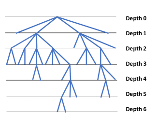
(b)

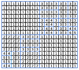
(c)

Figure 1: Example of (a) CTU partitioning in VVC and its corresponding (b) depth information and (c) depth map.

Nowadays, there are numerous algorithms developed to low complexity intra or inter prediction for HEVC, including non-learning and learning-based algorithms. There are still few contributions on complexity optimization of VVC.

II-A Low-Complexity HEVC Prediction without Learning

Researchers have developed various algorithms aiming at efficient CU partitioning on the HEVC standard [3, 4, 5, 6, 8, 11, 12, 13, 14, 15, 012, 16, 17, 18, 7, 9, 10]. Gu et al. [3] proposed an adaptive approach to boost intra prediction of HEVC, where the intra angular prediction modes and partition depth were predicted by the distribution of coding residual. In [4], Tsang et al. proposed to reduce the computational complexity of HEVC-based Screen Content Coding (SCC), in which the intrablock copy mode was also optimized. In [5], the rough mode decision candidate list and rate distortion optimization candidate list are narrowed by the spatial-temporal adjacent Prediction Unit (PU). Fernández et al. [6] employed Parseval’s relation and the Mean Absolute Deviation (MAD) of motion component to analyze the spatial and temporal homogeneity of video frames, which was further used in CU partition decision. Zhang et al. [7] proposed a probability-based early depth intra mode decision to speed up the time-consuming view synthesis optimization. Based on the Bayesian decision rule and scene change detection, Kuang et al. [8] proposed an online-learning method to reduce the computational complexity of encoder. Goswami et al. [9] used two Bayesian classifiers for early skip decision and CU termination respectively. The Markov Chain Monte Carlo method was applied to determine prior and class conditional probability values at run time. In [10], Xiong et al. modeled CU partition as a Markov random field and conducted a maximum a posteriori approach to evaluate the splittings of the CUs. Zhang et al. [11] developed a dynamic HEVC coding scheme that achieves a user-defined complexity constraint by adjusting the depth range for each CTU. Duanmu et al. [12] adopted extensive statistical studies and mode mapping techniques to early terminate the partitioning process of CU. The work in [13] used the depth information of previously coded CUs to adaptively choose the optimal CU depth range. Shen et al. [14] skipped the unnecessary CU depth levels and intra angular prediction modes by using the information of upper depth level CUs and neighboring CUs. [15] predicted the RD cost of intra angular modes to skip the non-promising modes. Based on the distortion cost obtained from motion estimation, proposed a CU partitioning algorithm to speed up the coding process. In addition, the researchers have developed more than fast partition in HEVC. In [16] and [17], the fast intra and inter partition methods were extended to the scalable video encoders, while in [18], an improved RD model achieved its efficiency in Motion Estimation (ME) by introducing complexity optimization.

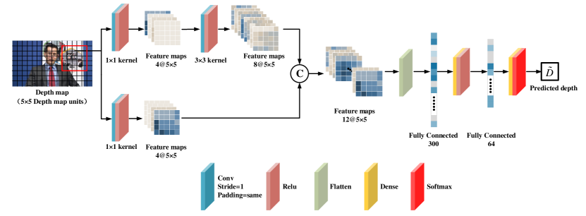
Figure 2: The architecture of the proposed D-DFF.

II-B Low-Complexity HEVC Prediction with Learning

The application of Machine Learning (ML) has become popular in video coding optimization. The application of ML-based algorithm brings extra computational load to the encoder, resulting in the increase of coding time. However, compared with the computational complexity of the encoder, the overhead of ML-based algorithm is negligible [19]. In [20], Mercat et al. demonstrated the superiority of ML-based method to conventional probability-based method in the scenario of fast video coding. As a popular tool in machine learning, the random forest was demonstrated to effectively predict the intra angular prediction mode by Ryu et al. [21]. In [22], Tsang et al. utilized the random forest to design mode skipping strategy for SCC, in order to reduce the computational complexity of intrablock copy and palette modes. Grellert et al. [23] proposed a Support Vector Machine (SVM) based method to make fast CU partition decision. In this method, the coding flags, coding metrics and motion cues were utilized as the inputs of SVM. The SVM-based models were also explored in [24, 25], which utilized the average number of contour points in current CU and the image texture complexity, respectively. [26] employed the CNN to analyze the luminance components of video frame, which was furthermore employed to determine the depth range of CTU. In [27], during the process of fast CU partition decision, CNN was used to decide whether an 8$\times$8 CU needs to be split. Yeh et al. [28] designed a simplified CNN structure and a complex CNN structure to enhance the performance of encoder on CPU and GPU, respectively. Li et al. [29] established a large-scale database of CU partition and applied a deep CNN to make binary decision for CU partition. This work was further improved in [19] by introducing the Long-Short-Term-Memory (LSTM) network. In addition, high-level image features have also been adopted in CNN-based fast CU partition. For example, in [30], Kuanar et al. embedded region-wise image features in their CNN model. Kim et al. [31] jointly used the image and features extracted from the coding process (e.g. PU modes, intra angular prediction modes, motion vector) to train the CNN model.

II-C Low-Complexity VVC Optimization

Despite of the above great efforts, they were all designed for the HEVC standard, lacking of application in the newly released VVC. To further exploit the potentiality of video compression, the VVC adopts a more complex QuadTree with nested Multi-type Tree (QTMT) structure, as shown in Fig. 1 (a,b). As a result, the above approaches cannot be directly applied in VVC and thus new optimization approaches are required. Cui et al. [32] proposed an early termination algorithm based on horizontal and vertical gradients to pre-determine binary partition or ternary partition. Variance and Sobel operator were used in [33] to terminate further partition of 32$\times$32 CU and decide QTMT structure. Wang et al. [34] employed the residual block as the input of CNN to predict the CU depth and also accelerated the inter coding process. In [35], the inherent texture richness of the image was adopted in CNN to predict the partition depth range of 32$\times$32 block. [36] utilized two CNNs to predict boundaries for luma and chroma components, respectively. Based on random forest, [37] designed a Quad Tree Binary Tree partitioning scheme to determine the most probable partition modes for each coding block. [38] extracted texture region features based on gray-level co-occurrence matrix to train random forest classifier, which predicts CU partition. To improve the flexible QTMT structure, [39] proposed a multi-stage CU partition by a CNN model trained with an adaptive loss function. Li et al. [40] established two decision models by exploiting the hierarchal correlation of the luma prediction distortion for early skipping Binary Tree (BT) and Ternary Tree (TT) partition. To reduce encoding complexity, Wu et al. [41] trained split classifier and splitting directional classifier based on SVM for different sizes of CUs. In [42], a Context-based Ternary Trees Decision (C-TTD) approach was proposed to skip the TT partitions which efficiently reduced the encoding time. Fu et al. [43] adopted Bayesian rule to early skip the splitting of CU, in which the split types and intra prediction modes of children CUs were used. Yang et al. [44] proposed a CTU Structure Decision Strategy based on Statistical Learning (CSD-SL) and a fast intra mode decision method for VVC intra coding. Tang et al. [45] used the block-level based Canny edge detector to extract edge features to skip vertical or horizonal partition modes. According to the edge map, the homogenous CUs can be early terminated.

III The Proposed Algorithm

In the state-of-the-art VVC intra prediction, there are two steps that are successively executed. Firstly, the CTU is iteratively split into a number of CUs with different coding depth. Secondly, in each coding depth, the partition modes with different directions and patterns are thoroughly checked to find the one with the minimum RD cost. Accordingly, we also design a two-stage complexity optimization strategy: the D-DFF to determine the optimal depth and the P-PBE to select the candidate partitions. The chosen depth and partitions are finally used to speed up the CU partition process in VVC intra coding.

III-A Intra Depth Prediction with Deep Feature Fusion

To support videos with higher definition and fidelity, the VVC incorporates larger size and depth of CTU, as compared with HEVC. The complicated CTU structure requires an efficient method to reduce its computational cost. In this work, we divide the CTU into 8$\times$8 blocks and make an attempt to predict the optimal depth of each block. The selection of block size 8$\times$8 is based on a tradeoff between prediction accuracy and coding complexity. As shown in Fig. 1 (c), a CTU of size 128$\times$128 is divided into 16$\times$16 blocks.

To accurately predict the optimal depth values, we need to collect the reference information that is available during video coding. The strong spatial-temporal correlation [15] inspires us to adopt the depth information of spatial-temporal neighboring CUs. For each 8$\times$8 block located at $(x,y,t)$, where $x,y$ and $t$ respectively denote the spatial coordinates and temporal order, we collect depth values of the following blocks:

$$\begin{split}S_{D}=\begin{cases}B(x+\Delta x,y+\Delta y,t),\\ \qquad\quad\qquad{\text{\text{i}f }\Delta x<0||\Delta x=0\&\Delta y<0},\ \\ B(x+\Delta x,y+\Delta y,t-1),\qquad{\text{otherwise}},\ \end{cases}\end{split}$$ (1)

where $\Delta x$ and $\Delta y$ denote the integers ranging from -2 to 2. In other words, we collect the depth of a neighboring block if it has been coded; otherwise, we collect the depth of its co-located block at the previously coded frame.

We extract and fuse the features of these spatial-temporal references with a deep CNN. In particular, the CNN is designed as a lightweight network with multi-scale feature fusion. The lightweight network avoids high computational overhead. The multi-scale feature fusion obtained with different sizes of convolutional kernels provides more accurate classification than single scale features [46]. The network infrastructure, training and depth prediction are elaborated as follows.

1) Network Infrastructure

The design of proposed model is inspired by the inception module, which was proposed to solve complex image recognition and classification tasks. To avoid large computational overhead, we set the model with reduced parameters and dimensions. As shown in Fig. 2, the proposed D-DFF consists of three steps: feature extraction, feature concatenation and classification.

The feature extraction step receives the reference depth map defined in (1). It extracts the features of depth map in two paths: one utilizes a 1$\times$1 convolutional kernel for dimension promotion and a 3$\times$3 convolutional kernel with ReLU for scaled feature extraction; the other utilizes a 1$\times$1 kernel only. With $\Delta x$ and $\Delta y$ ranging from -2 to 2, the size of depth map is 5$\times$5. The two paths output 8 and 4 5$\times$5 feature maps, respectively. All extracted features are input to the next step for feature fusion.

The feature concatenation step combines all feature maps from the first step and flattens them into a vector. For each depth unit, the 1$\times$1 convolution kernel is equivalent to the unit performing fully connected calculations on all features. Connecting multiple convolutions in series in the same size receptive field benefits the combination of more nonlinear features and extract richer features [46]. After this step, the 12 5$\times$5 feature maps are stretched into a vector of length 300.

Finally, the classification step receives the feature vectors and outputs the predicted depth ${\tilde{{D}}(x,y)}$. A neural network with 2 hidden layers and a softmax layer is employed to fulfill this task. Since the intra prediction is performed at CU depth 1 or above, there are only 6 types of output depth from 1 to 6. The depth value with the highest probability is selected as the predicted depth.

Aimed at a tradeoff between model accuracy and complexity, we have optimized all hyper-parameters of this D-DFF model. An important design of this model is its two-path feature extraction to obtain multi-scale features. In this step, the maximum number of convolutional layers influences both the prediction accuracy and the computational overhead of our model. In Fig. 3, we present the average accuracy and overhead of our model under different number of 3$\times$3 convolutional layers. Four typical video sequences (BQTerrace, RaceHorsesC, BQSquare and Johnny) are tested with Qp from 22 to 37. From the figure, the model with one 3$\times$3 convolutional layer achieves a good tradeoff between model accuracy and computational complexity. As a result, we utilize a 1$\times$1 and a 3$\times$3 convolutional layer in the first path. The maximum number of convolutional layers are set as 2.

Figure 3: The model accuracy and computational overhead under different number of 3$\times$3 convolutional layers.

2) Model Training

We collect 58 video sequences from the LIVE data set [47], the UVG data set [48] and the standard sequences of AVS2/AVS3. As shown in Table I, these sequences cover a large range of resolutions with diversified frame rates and bit depths. As shown in Fig. 4, they also cover a wide range of Spatial Information (SI) and Temporal Information (TI). These sequences are further compressed by VTM 12.0 with 4 Quantization parameters (Qps) of 22, 27, 32 and 37. Therefore, these compressed sequences are representative to improve the generalization performance of our prediction model.

TABLE I: The video sequences for model training and testing

Sources	Resolution	Number of sequences	Frame rate	Bit depth
UVG	3840$\times$2160	8	50	10
	1920$\times$1080	8	50	8
AVS2	3840$\times$2160	2	50	10
	2560$\times$1600	1	30	8
	1920$\times$1080	7	25	8
	1280$\times$720	5	60	8
AVS3	3840$\times$2160	6	30	10
	1280$\times$720	5	30	8
	720$\times$1280	3	30	8
	640$\times$360	3	30	8
LIVE	1280$\times$720	10	24	8

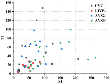
Figure 4: The SI and TI distributions of sequences in Table I .

During the compression, we collect all depth values of CUs and reorganize them into pairs of the predicted depths and the corresponding reference depth maps. These data pairs formulate a big dataset which is further divided into a training and a testing set at a 4:1 ratio. For training, we set the batch size and the iterations as 256 and 128, respectively. We choose Adam optimizer with a learning rate of 0.0001. The cross entropy function, which is popular in classification, is utilized as the loss function.

Our deep model demonstrates high prediction performance in the testing set. As shown in Fig. 5, $2351539/2575967=91.29\%$ depth values are correctly predicted with another $219901/2575967=8.54\%$ within the error of ${\pm 1}$. As shown in Table II, the proposed model achieves the average precision, recall, specificity and accuracy of 0.914, 0.917, 0.983 and 0.971, respectively. These results demonstrate the effectiveness of our model, especially when considering its lightweight infrastructure.

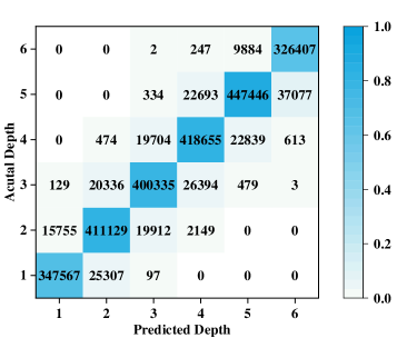
Figure 5: The heat map of our depth prediction model.

TABLE II: The classification performance of our depth prediction model

Depth	Precision	Recall	Specificity	Accuracy
1	0.956	0.932	0.993	0.984
2	0.900	0.916	0.978	0.967
3	0.909	0.894	0.981	0.966
4	0.890	0.906	0.976	0.963
5	0.931	0.882	0.984	0.964
6	0.896	0.970	0.983	0.981
Average	0.914	0.917	0.983	0.971

3) The Depth Prediction

Our deep model achieves a tradeoff between the prediction accuracy and the computational overhead. However, in video coding optimization, a tradeoff shall be achieved between the finally achieved RD performance and the overall computational complexity. Hence, there exists a gap between the two tradeoffs. The first tradeoff chooses the most probable depth, which may still lead to a small portion of incorrect prediction. These incorrect predictions may accumulate to a considerable quantity during video coding and further result in an intolerable increment of RD cost. To avoid this error propagation, we employ a conservative strategy as follows:

$$\begin{split}{\hat{D}(x,y)}=&{\tilde{D}(x,y)}+\\ &\max\{\lfloor\frac{1}{{K}_{D}}\sum\limits_{k=1}^{{K}_{D}}({D}_{k}(x,y)-\tilde{{D}_{k}}(x,y))+\frac{1}{2}\rfloor,0\},\end{split}$$ (2)

where $\hat{D}(x,y)$ represents the adjusted depth. $K_{D}=25$ denotes the number of reference blocks to predict the current depth. $D_{k}(x,y)$ and $\tilde{D}_{k}(x,y)$ represent the final and predicted depth of $k$-th reference block. Through (2), we are able to estimate a depth offset from its neighboring blocks. This method effectively reduces the RD loss caused by accumulated prediction error and further improves the robustness of our D-DFF model.

We can derive the optimal depth of each CU based on the adjusted depth $\hat{D}(x,y)$. In a CU with multiple 8$\times$8 blocks, its optimal coding depth is estimated as

$${D}_{o}=\max\limits_{\{x,y\}\in\text{CU}}\{\hat{D}(x,y)\}.$$ (3)

During coding, the current CU is iteratively split until its optimal depth. The coding depth larger than the optimal depth is skipped to save the coding time.

III-B Intra Partition Mode Prediction with Probability Estimation

In CTU coding, the splitting process is iteratively performed until the optimal depth $D_{o}$ of each CU. For each depth less than $D_{o}$, the CU traverses 5 possible partition modes, including Quadtree (QT) partition, Vertical Binary Tree (BTV) partition, Horizontal Binary Tree (BTH) partition, Vertical Ternary Tree (TTV) splitting and Horizontal Ternary Tree (TTH) splitting. To further skip the unnecessary coding modes, we need to predict the probability of all mode partitions. As indicated above, the spatial-temporal correlation and reference mode partitions could be investigated for partition mode prediction.

Denote a CU located at $(x,y,t)$ as $U(x,y,t)$, whose size is larger than 4$\times$4 in VVC. We set its reference set as

$$\begin{split}S_{P}=\begin{cases}U(x+\Delta x,y+\Delta y,t||t-1),\\ \qquad\quad\qquad{\text{\text{i}f }\Delta x<0||\Delta x=0\&\Delta y<0},\ \\ U(x+\Delta x,y+\Delta y,t-1),\qquad{\text{otherwise}},\ \end{cases}\end{split}$$ (4)

where $\Delta x$ and $\Delta y$ ranges from -1 to 1. The reference set (4) is similar to (1) but with two differences. Firstly, we collect the partitions of top and left CUs in both the current and the left frames. Previous works showed that all these CUs have high partition correlations to the current CU [50], which inspires us to add all these CUs in the reference set $S_{P}$. Meanwhile, the probability-based partition prediction does not require a neat matrix for convolution, which also allows us to add these CUs. Secondly, the ranges of $\Delta x$ and $\Delta y$ are reduced. Without the convolutional operation, a smaller but effective reference set is more practical.

Let $R$ denote the set that consists of all best partitions modes in the reference CU set $S_{P}$, $R=\{{\rm bm}_{U}|U\in S_{p}\}$. For a partition mode $M$, its probability to be selected as the best partition mode can be estimated as:

$$P(\text{bm}=M)=P(\text{bm}=M|M\in R)P(M\in R)$$ (5)

$$+P(\text{bm}=M|M\notin R)P(M\notin R),$$

where $P(M\in R)$ and $P(M\notin R)$ are posterior probabilities that are either 0 or 1. Experimental results in Table III also shows that $P({\rm bm}=M|M\in R)\gg P({\rm bm}=M|M\notin R)$, where four typical sequences from the standard sequences of AVS2/AVS3 with different resolutions and Qps from 22 to 37 are examined. Here it is reasonable to set

$$P(\text{bm}=M|M\notin R)\approx 0,$$ (6)

which simplifies our derivation. The other part of (5) can be easily derived as

$$P(\text{bm}=M|M\in R)=\frac{\int_{U\in S_{P}}{P(bm_{U}=M)}}{\int_{m\in R}\int_{U\in S_{P}}{P(bm_{U}=m)}},$$ (7)

where $S_{p}$ and $R$ denote the reference CU and partition sets, as indicated above. In practice, the probabilities in (6) are estimated with the number of occurrences in coding history:

$$P(\text{bm}=M|M\in R)=\frac{\sum\limits_{U\in S_{P}}{N(bm_{U}=M)}}{\sum\limits_{m\in R}\sum\limits_{U\in S_{P}}{N(bm_{U}=m)}},$$ (8)

where $N(\cdot)$ indicates the statistical frequency of an event. Experimental results in the following demonstrate the effectiveness of our method.

TABLE III: The average probabilities to be the best partition mode

Sequences	Average Probabilities(%)
	$P(\text{bm}=M|M\in R)$	$P(\text{bm}=M|M\notin R)$
Pedestrian_area	36.74	8.16
Yellowflower	36.36	7.14
Night	36.24	4.65
ShuttleStart	36.88	6.94

After obtaining the probability of each partition mode, we sort the partition modes which belong to $R$ according to their descending probabilities and add the other modes (not in $R$) after them. When the RD cost of current partition mode ($J_{\rm cur}$) is larger than the minimum RD cost obtained so far ($J_{\rm min}$) , we skip the untested partitions to save the total encoding time. The flowchart of the proposed intra partition mode prediction, namely P-PBE, is shown in Fig. 6.

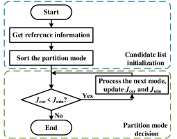
Figure 6: The proposed P-PBE method.

TABLE IV: Results of the proposed algorithm compared with the state-of-the-arts

Class	Sequences	C-TTD [42]		Fu’s [43]		CSD-SL [44]		Tang’s [45]		Proposed
		ATS($\%$)	BDBR($\%$)	ATS($\%$)	BDBR($\%$)	ATS($\%$)	BDBR($\%$)	ATS($\%$)	BDBR($\%$)	ATS($\%$)	BDBR($\%$)
A1	Tango	35.32	0.80	49.22	1.53	46.81	0.77	41.78	0.69	67.02	1.33
	FoodMarket4	29.39	0.77	50.29	0.95	50.88	0.53	32.08	0.53	53.17	0.97
	Campfire	35.32	0.61	53.51	0.90	42.11	0.83	34.37	0.98	57.32	1.56
	Average	33.34	0.73	51.01	1.13	46.60	0.71	36.08	0.73	59.17	1.29
A2	CatRobot	28.66	1.04	36.84	1.26	43.64	0.84	38.48	0.92	63.18	1.63
	DaylightRoad2	30.55	1.20	40.13	1.29	58.75	0.41	39.04	0.68	62.88	1.23
	ParkRunning3	33.50	0.54	48.03	0.44	51.76	0.62	34.66	0.58	59.52	0.88
	Average	30.90	0.93	41.67	0.99	51.38	0.63	37.39	0.73	61.86	1.25
B	BasketballDrive	25.68	0.90	45.37	0.85	58.43	1.58	45.61	0.93	60.35	1.53
	BQTerrace	27.42	0.73	47.28	0.85	56.22	2.14	36.64	0.84	56.19	1.16
	Cactus	27.55	0.75	48.91	1.29	59.94	2.06	39.51	0.91	62.98	1.78
	Kimono	28.17	0.82	47.39	1.10	57.95	1.42	32.69	0.44	67.04	0.93
	ParkScene	25.60	0.76	46.98	0.90	54.88	1.18	41.95	0.56	59.66	1.47
	Average	26.89	0.79	47.19	1.00	57.48	1.68	39.28	0.73	61.25	1.37
C	BasketballDrill	29.12	1.19	41.39	1.81	46.08	1.89	29.28	1.21	48.91	1.99
	BQMall	30.98	1.05	40.64	0.92	50.28	1.86	37.73	0.91	51.22	2.02
	PartyScene	39.17	0.61	40.14	0.40	49.06	0.76	35.68	0.41	49.86	0.87
	RaceHorsesC	38.52	0.64	46.38	0.75	44.96	1.06	32.62	0.61	49.98	1.27
	Average	34.45	0.87	42.14	0.97	47.59	1.39	33.83	0.79	49.99	1.54
D	BasketballPass	28.49	0.84	40.10	0.83	48.93	2.53	30.78	0.51	43.62	1.54
	BlowingBubbles	28.31	0.71	43.14	0.84	35.31	0.72	30.88	0.26	39.74	0.91
	BQSquare	35.89	0.51	44.20	0.56	44.16	0.79	27.53	0.23	45.31	0.79
	RaceHorses	30.49	0.77	45.36	0.97	47.08	0.85	26.63	0.33	48.93	1.09
	Average	30.79	0.71	43.20	0.80	43.87	1.22	28.95	0.33	44.40	1.08
E	FourPeople	29.00	1.08	41.79	1.60	58.85	2.82	44.29	1.31	58.45	1.97
	Johnny	31.59	0.99	40.11	1.38	55.63	3.32	39.96	1.21	59.37	2.05
	KristenAndSara	32.18	0.91	37.24	1.14	60.20	2.70	40.14	1.02	58.21	1.90
	Average	30.92	1.00	39.71	1.37	58.23	2.95	41.46	1.18	58.67	1.97
Total Average		30.95	0.83	44.29	1.03	50.99	1.44	36.01	0.73	55.59	1.40

III-C The Overall Algorithm

The overall algorithm is proposed as a two-stage method with D-DFF and P-PBE, which address the complexity optimizations at depth and partition levels, respectively. In particular, our method exploits the coding information of reference blocks and CUs, which are not always available for all cases. For D-DFF, an incomplete reference set $S_{D}$ cannot be processed by convolutions. In such case, the optimal depth $D_{o}$ of a CU is set as the same as that in its previously co-located CU. For P-PBE, an incomplete reference set still works to derive the probabilities. Therefore, the derivations in (6,7,8) can be processed during coding.

We summarize the steps of our algorithm as follows:

• For the first frame of each video sequence, encode the CUs with original encoder. Go to Step 2.

• Obtain the reference depth map $S_{D}$ and predict the depth with our CNN model. For each CU in this CTU determine its optimal depth $D_{o}$ with (3). Go to Step 3.

• Check the CTU coding iteratively. Once the current depth of CU exceeds its optimal depth, terminate the encoding process of this CU; otherwise, go to Step 4.

• For each coding depth, initialize the reference partition set $S_{P}$. Sort the partition modes in $R$ by (8) and add the remaining modes after them. Go to Step 5.

• Check the partition modes sequentially. If the current RD cost $J_{\rm cur}$ is larger than the minimum RD cost obtained so far $J_{\rm min}$, terminate the partition selection process and go to Step 4 for the next CU. If all CUs within this CTU has been checked, go to Step 2 to process the next CTU.

IV Experimental Results

To verify the effectiveness of our proposed algorithm, we implement it on the VTM-12.0 platform [51] under JVET Common Test Condition (CTC) [52] with ALL-INTRA configurations. The CTC provides 6 groups of video sequences, including A1 (3840$\times$2160), A2 (3840$\times$2160), B (1920$\times$1080), C (832$\times$480), D (416$\times$240) and E (1280$\times$720). These sequences are with a variety of Spatial Information (SI) and Temporal Information (TI) values [49], as demonstrated in Fig. 7. Therefore, the comprehensive examinations are sufficiently representative to examine the proposed algorithm.

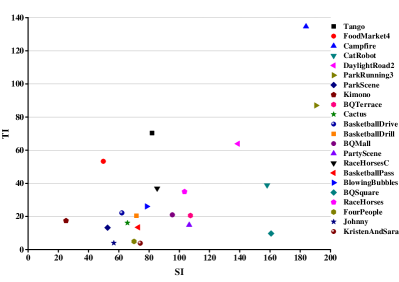
Figure 7: The distributions of SI and TI for all CTC sequences.

We compare the proposed algorithm and state-of-the-arts including C-TTD [42], Fu’s [43] , CSD-SL [44] and Tang’s [45]. The evaluation criteria include the Bjøntegaard Delta Bit Rate (BDBR) ($\%$) and the Average Time Saving (ATS) ($\%$) under four Qps (22, 27, 32 and 37), in which BDBR is defined in [53], and ATS is defined as

$$ATS=\frac{1}{4}\times\sum\limits_{i\in F}\frac{T_{\text{ori}}(i)-T_{\text{pro}}(i)}{T_{\text{ori}}(i)}\times 100\%,$$ (9)

where ${T_{\text{ori}}(i)}$ and ${T_{\text{pro}}(i)}$ respectively denote the encoding time of the original encoder and a proposed algorithm when encoding Qp is $i$. $F$ represents the Qp set above. An algorithm with lower BDBR or higher ATS is considered as a superior algorithm.

IV-A Comparison results with other benchmarks

The comparison results are shown in Table IV. The four comparison algorithms are implemented in different VTM versions. For fair comparison, we transplant their algorithms to VTM-12.0. All sequences from standard set are examined.

From Table IV, our scheme has superior computational complexity reduction compared to the other algorithms. The maximum time reduction occurs at Kimono sequence. Kimono has large smooth area with slow motion, thus few CTUs in Kimono need to be deeply split in our algorithm. On the contrary, the least time reduction is achieved when encoding BlowingBubbles. The reason mainly lies in its complex textures. In addition, videos with intense motion (e.g. BasketballDrill) have low correlation between neighboring CU depth map units. It reduces the prediction accuracy of the proposed algorithm, resulting in large coding bit-rate increase.

The other three algorithms, C-TTD [42], Fu’s [43] and Tang’s [45], achieve lower BDBR losses. However, their average encoding time savings are limited at 30.95$\%$, 44.29$\%$ and 36.01$\%$, respectively. On the other hand, the proposed method reduces the computational complexity of encoder by 55.59$\%$ with 1.40$\%$ BDBR increment. Thus, the proposed method further accelerates the encoding speed with acceptable coding loss.

Compared with CSD-SL [44], our algorithm improves 0.04% in BDBR and 3.60% in ATS. Firstly, for Class A1 and A2, our method focuses on improving ATS, which can save up to 20.21% more coding time than CSD-SL. Secondly, for the Class B, our method outperforms in both ATS and BDBR. Thirdly, for the Class E, our method can save 0.98% more bit rate under the same coding time. In addition, our algorithm also has the following advantages. i) It extracts relatively concise features and uses relatively less network parameters, without tedious calculations. ii) It utilizes a uniform network model for different partition modes, which is easier to be implemented than other methods such as CSD-SL. iii) It has more time saving in HD and UHD videos (e.g. Class A1, Class A2 and Class B), which is favorable under the booming of HD and UHD in videos.

The performance of our proposed algorithm are benefited from two modules. Firstly, the D-DFF effectively terminates the iterative partition process, by utilizing a lightweight CNN to predict an optimal coding depth. Secondly, at each depth, the P-PBE effectively skips the unnecessary partition methods, by exploiting the neighboring coding information. In conclusion, the proposed algorithm achieves better encoding time reduction compared with other four algorithms with slight BDBR loss and simple implementation structure.

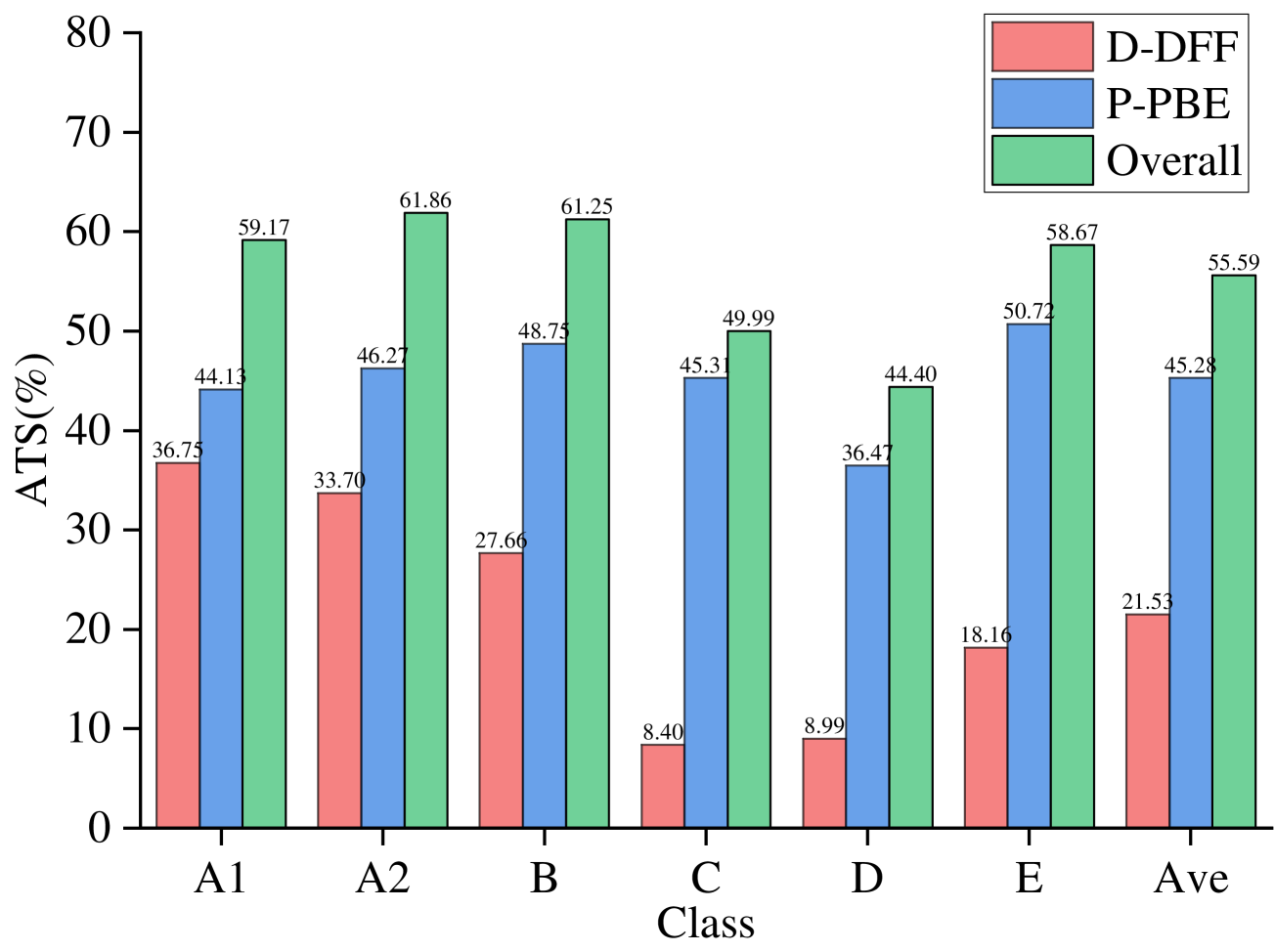
(a)

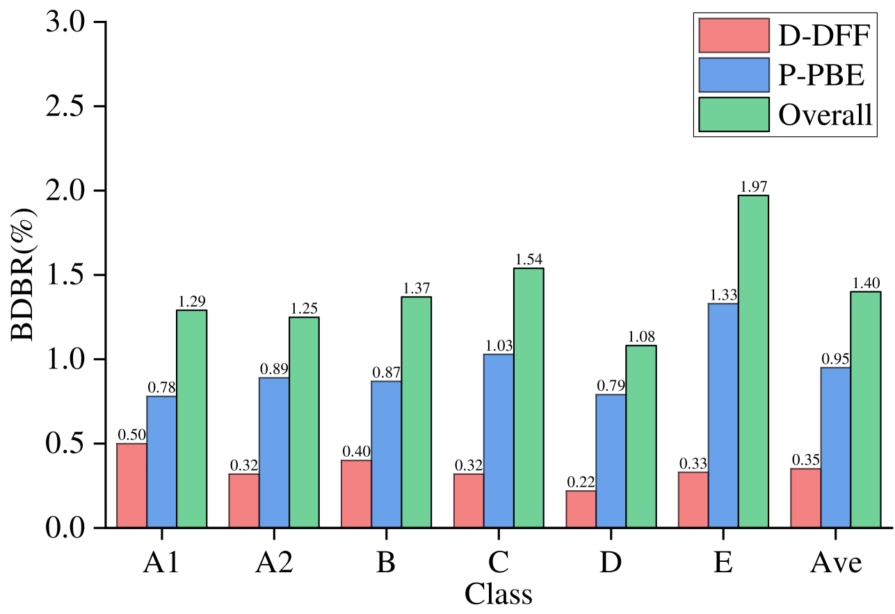
(b)

Figure 8: Results of ablation experiments in terms of (a) ATS and (b) BDBR.

IV-B Additional analysis

To analyze the contributions of individual parts, we conduct ablation experiments with results shown in Fig. 8. The D-DFF model achieves 21.53$\%$ encoding time reduction with negligible BDBR loss. Moreover, the encoding time reduction performances of the D-DFF model in HD and UHD sequences (e.g. Class A1, Class A2, Class B) are more significant than that in lower resolution videos. The encoding time reduction of the P-PBE model remains relatively stable in all sequences with 0.95$\%$ BDBR. Furthermore, the overall algorithm, which incorporates the D-DFF and the P-PBE models, achieves 55.59$\%$ complexity reduction with a tolerable RD loss of 1.40% on average.

To analyze the sensitivity of the proposed algorithm with respect to Qp values, we test the time reductions of our algorithm under different Qps and show them in Fig. 9. It can be observed that the proposed algorithm achieves consistent time saving over different Qps. Therefore, our method is more robust to the changes of coding parameters.

For completeness, we also analyze the overhead of the proposed algorithm in encoder. Fig. 10 shows the overhead of proposed algorithm under different classes and Qps. Generally, the overhead is generally less than 1.8$\%$, with an average value of 0.48%. With higher Qp values, the overhead proportion tends to be increased due to the decrease of overall coding complexity. In general, the overhead can be ignored compared with its benefits in overall time reduction.

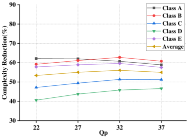
Figure 9: The complexity reduction of different classes under different Qps.

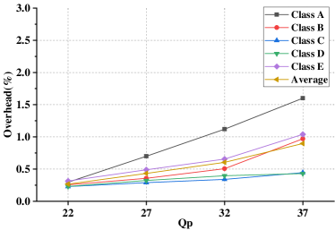
Figure 10: The overhead of proposed algorithm under different classes and Qps.

V Conclusion

This paper addresses the problem of efficient VVC intra coding. First, we propose a CNN-driven CU depth prediction model and the predicted depth map is used to check early CU termination. Then, the candidate partition modes are further determined through probability estimation to save more encoding time. This two-stage approach has a great efficiency of time reduction compared with state-of-the-arts with negligible RD performance loss, offering 55.59$\%$ encoding complexity reduction on average. The whole framework is also applicable in VVC inter prediction with depth-based CU partition. We put it as a future work.

References

- [1] Cisco visual networking index : Forecast and methodology, 2017-2022. [Online]. Available:https://www.cisco.com/c/en/us/solutions/collateral/service-provider/visual-networking-index-vni/white-paper-c11-741490.html.
- [2] B. Bross, Y. Wang, Y. Ye, S. Liu, J. Chen, G.J. Sullivan and J. Ohm, “Overview of the Versatile Video Coding (VVC) Standard and its Applications,” IEEE Trans. Circuits Sys. Video Technol., vol. 31, no. 10, pp. 3736–3764, Oct. 2021.
- [3] J. Gu, M. Tang, J. Wen, and Y. Han, “Adaptive intra candidate selection with early depth decision for fast intra prediction in HEVC,” IEEE Signal Process. Lett., vol. 25, no. 2, pp. 159–163, Feb. 2018.
- [4] S. Tsang, Y. Chan, W. Kuang, and W. Siu, “Reduced-complexity intra block copy (IntraBC) mode with early CU splitting and pruning for HEVC screen content coding,” IEEE Trans. Multimedia., vol. 21, no. 2, pp. 269-283, Feb. 2019.
- [5] K. Duan, P. Liu, Z. Feng, and K. Jia, “Fast PU intra mode decision in intra HEVC coding,” Data Compress. Conf. (DCC’19), pp. 570–570, Mar. 2019.
- [6] D. G. Fernández, A. A. Del Barrio, G. Botella, and C. García, “Fast and effective CU size decision based on spatial and temporal homogeneity detection,” Multimedia Tools Appl., vol. 77, no. 5, pp. 5907–5927, Mar. 2018.
- [7] H. Zhang, C. Fu, Y. Chan, S. Tsang and W. Siu, “Probability-Based Depth Intra-Mode Skipping Strategy and Novel VSO Metric for DMM Decision in 3D-HEVC,” IEEE Trans. Circuits Sys. Video Technol., vol. 28, no. 2, pp. 513–527, Feb. 2018.
- [8] W. Kuang, Y. Chan, S. Tsang, and W. Siu, “Online-learning-based Bayesian decision rule for fast intra mode and CU partitioning algorithm in HEVC screen content coding,” IEEE Trans. Image Process., vol. 26, no. 1, pp. 170-185, Jul. 2019.
- [9] K. Goswami, and B. Kim, “A Design of Fast High Efficiency Video Coding (HEVC) Scheme Based on Markov Chain Monte Carlo Model and Bayesian Classifier,” IEEE Trans. Ind. Electron. Control Instrum., vol. 65, no. 11, pp. 8861-8871, Nov. 2018.
- [10] J. Xiong, H. Li, F. Meng, S. Zhu, Q. Wu and B. Zeng, “MRF-Based Fast HEVC Inter CU Decision With the Variance of Absolute Differences,” IEEE Trans. Multimedia., vol. 16, no. 8, pp. 2141-2153, Dec. 2014.
- [11] J. Zhang, S. Kwong, T. Zhao, and Z. Pan, “CTU-level complexity control for High Efficiency Video Coding,” IEEE Trans. Multimedia., vol. 20, no. 1, pp. 29-44, Jan. 2018.
- [12] F. Duanmu, Z. Ma, M. Xu, and Y. Wang, “An HEVC-compliant fast screen content transcoding framework based on mode mapping,” IEEE Trans. Circuits Sys. Video Technol., vol. 29, no. 10, pp. 3068–3082, Oct. 2019.
- [13] J. H. Bae and M. H. Sunwoo, “Adaptive early termination algorithm using coding unit depth history in HEVC,” J. Signal Process. Sys., vol. 91, no. 8, pp. 863–873, Aug. 2019.
- [14] L. Shen, Z. Zhang, and P. An, “Fast CU size decision and mode decision algorithm for HEVC intra coding,” IEEE Trans. Consumer Electron., vol. 59, no. 1, pp. 207–213, Feb. 2013.
- [15] M. Jamali and S. Coulombe, “Fast HEVC intra mode decision based on RDO cost prediction,” IEEE Trans. Broadcast., vol. 65, no. 1, pp. 109–122, Mar. 2019.
- [16] L. Shen and G. Feng, “Content-based adaptive SHVC mode decision algorithm,” IEEE Trans. Multimedia., vol. 21, no. 11, pp. 2714–2725, Nov. 2019.
- [17] D. Wang, Y. Sun, C. Zhu, W. Li, and F. Dufaux, “Fast depth and inter mode prediction for quality scalable High Efficiency Video Coding,” IEEE Trans. Multimedia., vol. 22, no. 4, pp. 833–845, Apr. 2020.
- [18] L. Jia, C. Tsui, O.C. Au, and K. Jia, “A new rate-complexity-distortion model for fast motion estimation algorithm in HEVC,” IEEE Trans. Multimedia., vol. 21, no. 4, pp. 835–850, Apr. 2019.
- [19] M. Xu, T. Li, Z. Wang, X. Deng, R. Yang, and Z. Guan, “Reducing complexity of HEVC: a deep learning approach,” IEEE Trans. Image Process., vol. 27, no. 10, pp. 5044–5059, Oct. 2018.
- [20] A. Mercat, F. Arrestier, M. Pelcat, W. Hamidouche, and D. Menard, “Probabilistic approach versus machine learning for one-shot quad-tree prediction in an intra HEVC encoder,” J. Signal Process. Sys., vol. 91, no. 9, pp. 1021–1037, Sept. 2019.
- [21] S. Ryu and J. Kang, “Machine learning-based fast angular prediction mode decision technique in video coding,” IEEE Trans. Image Process., vol. 27, no. 11, pp. 5525–5538, Nov. 2018.
- [22] S. Tsang, Y. Chan, and W. Kuang, “Mode skipping for HEVC screen content coding via random forest,” IEEE Trans. Multimedia., vol. 21, no. 10, pp. 2433–2446, Oct. 2019.
- [23] M. Grellert, B. Zatt, S. Bampi, and L. A. da Silva Cruz, “Fast coding unit partition decision for HEVC using support vector machines,” IEEE Trans. Circuits Sys. Video Technol., vol. 29, no. 6, pp. 1741–1753, Jun. 2019.
- [24] C. Sun, X. Fan, and D. Zhao, “A fast intra CU size decision algorithm based on canny operator and SVM classifier,” in IEEE Int. Conf. Image Process. (ICIP’18), pp. 1787–1791, Oct. 2018.
- [25] X. Liu, Y. Li, D. Liu, P. Wang, and L. T. Yang, “An adaptive CU size decision algorithm for HEVC intra prediction based on complexity classification using machine learning,” IEEE Trans. Circuits Sys. Video Technol., vol. 29, no. 1, pp. 144–155, Jan. 2019.
- [26] Z. Feng, P. Liu, K. Jia, and K. Duan, “Fast intra CTU depth decision for HEVC,” IEEE Access, vol. 6, pp. 45 262–45 269, Aug. 2018.
- [27] K. Chen, X. Zeng, and Y. Fan, “CNN oriented fast CU partition decision and PU mode decision for HEVC intra encoding,” in Int. Conf. Solid-State Integr. Circuit Technol. (ICSICT’18), pp. 1–3, Oct. 2018.
- [28] C. Yeh, Z. Zhang, M. Chen, and C. Lin, “HEVC intra frame coding based on convolutional neural network,” IEEE Access, vol. 6, pp. 50 087–50 095, Aug. 2018.
- [29] T. Li, M. Xu, and X. Deng, “A deep convolutional neural network approach for complexity reduction on intra-mode HEVC,” in IEEE Int. Conf. Multimedia & Expo (ICME’17), pp. 1255–1260, Jul. 2017.
- [30] S. Kuanar, K. R. Rao, and C. Conly, “Fast mode decision in HEVC intra prediction, using region wise CNN feature classification,” in IEEE Int. Conf. Multimedia & Expo Workshops (ICMEW’18), pp. 1–4, Jul. 2018. 2018.
- [31] K. Kim and W. W. Ro, “Fast CU depth decision for HEVC using neural networks,” IEEE Trans. Circuits Sys. Video Technol., pp. 1–12, Aug. 2018.
- [32] J. Cui, T. Zhang, C. Gu, X. Zhang and S. Ma, “Gradient-Based Early Termination of CU Partition in VVC Intra Coding,” Data Compress. Conf. (DCC’20), pp. 103–112, Mar. 2020.
- [33] Y. Fan, J. Chen, H. Sun, J. Katto and M. Jing, “A Fast QTMT Partition Decision Strategy for VVC Intra Prediction,” IEEE Access, vol. 8, pp. 107900-107911, June. 2020.
- [34] Z. Wang, S. Wang, X. Zhang, S. Wang, and S. Ma, “Fast QTBT partitioning decision for interframe coding with convolution neural network,” IEEE Int. Conf. Image Process. (ICIP’18), pp. 2550-2554, Oct. 2018.
- [35] Z. Jin, P. An, C. Yang, and L. Shen, “Fast QTBT partition algorithm for intra frame coding through convolutional neural network,” IEEE Access, vol. 6, pp. 54660-54673, Oct. 2018.
- [36] F. Galpin, F. Racapé, S. Jaiswal, P. Bordes, F. Le Léannec, and E. François, “CNN-based driving of block partitioning for intra slices encoding,” Data Compress. Conf. (DCC’19), pp. 162-171, Mar. 2019.
- [37] T. Amestoy, A. Mercat, W. Hamidouche, D. Menard, and C. Bergeron, “Tunable VVC frame partitioning based on lightweight machine learning,” IEEE Trans. Image Process., vol. 29, pp. 1313–1328, Sept. 2019.
- [38] Q. Zhang, Y. Wang, L. Huang, and B. Jiang, “Fast CU Partition and Intra Mode Decision Method for H.266/VVC,” IEEE Access, vol. 8, pp. 117539–117550, June. 2020.
- [39] T. Li, X. Ma, R. Tang, Y. Chen, and Q. Xing, “DeepQTMT: A Deep Learning Approach for Fast QTMT-based CU Partition of Intra-mode VVC,” IEEE Trans. Image Process., vol. 30, pp. 5377–5399, May. 2021.
- [40] Y. Li, G. Yang, Y. Song, H. Zhang, X. Ding, and D. Zhang, “Early Intra CU Size Decision for Versatile Video Coding Based on a Tunable Decision Model,” IEEE Trans. Broadcast.,pp. 1–11, Apr. 2021.
- [41] G. Wu, Y. Huang, C. Zhu, L. Song, and W. Zhang, “SVM Based Fast CU Partitioning Algorithm for VVC Intra Coding,” in IEEE Int. Sym. Circuits Sys. (ISCAS’21), May. 2021.
- [42] S. Park and J. Kang, “Context-based ternary tree decision method in Versatile Video Coding for fast intra coding,” IEEE Access, vol. 7, pp.172597–172605, Nov. 2019.
- [43] T. Fu, H. Zhang, F. Mu, and H. Chen, “Fast CU partitioning algorithm for H.266/VVC intra-frame coding,” in IEEE Int. Conf. Multimedia & Expo (ICME’19), pp. 55–60, Jul. 2019.
- [44] H. Yang, L. Shen, X. Dong, Q. Ding, P. An, and G. Jiang, “Low complexity CTU partition structure decision and fast intra mode decision for versatile video coding,” IEEE Trans. Circuits Sys. Video Technol., pp. 1–14, Mar. 2019.
- [45] N. Tang, J. Cao, F. Liang, J. Wang, H. Liu , X. Wang, and X. Du, “Fast CTU partition decision algorithm for VVC intra and inter coding,” IEEE Asia Pac. Conf. Circuits Syst., pp. 361–364, Nov. 2019.
- [46] C. Szegedy, W. Liu, Y. Jia, P. Sermanet, S. Reed, D. Anguelov, D. Erhan, V. Vanhoucke and A. Rabinovich, “Going deeper with convolutions,” in IEEE Conference on Computer Vision and Pattern Recognition (CVPR’15), pp. 1-9, Jun. 2015.
- [47] G. Lu, W. Ouyang and D. Xu, “DVC: An End-to-end Deep Video Compression Framework,” in IEEE Conference on Computer Vision and Pattern Recognition (CVPR’19), pp. 10998-11007, Jun. 2019.
- [48] A. Moorthy, L. Choi and A. Bovik, “Video Quality Assessment on Mobile Devices: Subjective, Behavioral and Objective Studies,” in IEEE Journal of Selected Topics in Signal Processing, vol. 6, pp. 652-671, Oct. 2012.
- [49] Methodology for the subjective assessment of video quality in multimedia applications, ITU-T P.910, International Telecommunication Union, 1999.
- [50] T. Zhao, H. Wang, S. Kwong, and S. Hu, “Probability-based coding mode prediction for H.264/AVC,”IEEE Int. Conf. Image Process. (ICIP’10), pp. 3389-3392, Sept. 2010.
- [51] VTM-12.0. [Online]. Available:https://vcgit.hhi.fraunhofer.de/jvet/VVCSoftware_VTM/-/tree/VTM-12.0.
- [52] F. Bossen, J. Boyce, X. Li, V. Seregin, and K. Suehring, JVET common test conditions and software reference configurations for SDR video, document JVET-K1010-v2, Jul. 2018.
- [53] G. Bjontegaard, “Calculation of average PSNR differences between RD curves,” Proceedings of the ITU-T Video Coding Experts Group (VCEG) Thirteenth Meeting, Doc. VCEG-M33, Austin, TX, Apr. 2001.