Phonon-mediated Migdal effect in semiconductor detectors

Abstract

The Migdal effect inside detectors provides a new possibility of probing the sub-GeV dark matter (DM) particles. While there has been well-established methods treating the Migdal effect in isolated atoms, a coherent and complete description of the valence electrons in semiconductor is still absent. The bremstrahlung-like approach is a promising attempt, but it turns invalid for DM masses below a few tens of MeV. In this paper, we lay out a framework where phonon is chosen as an effective degree of freedom to describe the Migdal effect in semiconductors. In this picture, a valence electron is excited to the conduction state via exchange of a virtual phonon, accompanied by a multi-phonon process triggered by an incident DM particle. Under the incoherent approximation, it turns out that this approach can effectively push the sensitivities of the semiconductor targets further down to the MeV DM mass region.

1 Introduction

The search for low-mass dark matter (DM) particle has progressed tremendously in the past decade, with significant theoretical and experimental advances in new detection channels and materials [1], such as in semiconductors [2, 3, 4, 5], Dirac materials [6, 7, 8], superconductors [9, 10], superfluid helium [11, 12, 13], and via phonon excitations [14, 15, 16] and bremsstrahlung photons [17, 18], as well as other proposals and analyses [19, 20, 21, 22, 23, 24, 25, 26, 27, 28, 29, 30, 31, 32, 33, 34, 35, 36, 37, 38, 39, 40, 41, 42].

The Migdal effect has attracted wide interest recently because the study in Ref. [43] has shown that in theory the suddenly struck nucleus can produce ionized electrons more easily than anticipated for an incident sub-GeV DM particle, so exploring relevant parameter region is plausible for the present detection technologies. Although the Migdal effect has not been directly observed in a nuclear collision, attempts to make the first such measurement from neutron-nucleus scattering are underway [44, 45, 46]. After Ref. [43], there has emerged numerous theoretical proposals [43, 47, 48, 49, 18, 50, 51, 52, 53, 54, 55, 56] and experimental efforts dedicated to detecting the sub-GeV DM particles via the Migdal effect in liquids [57], and in condensed matter targets [58, 59, 60, 61].

Compared with the typical ionization energy thresholds in atoms $\varepsilon_{g}\sim\mathcal{O}\left(10\right)\,\mathrm{eV}$, semiconductor targets have a much lower thresholds $\varepsilon_{g}\sim\mathcal{O}\left(1\right)\,\mathrm{eV}$, which makes them ideal materials for further exploiting the the Migdal effect in the probe of light DM particles. However, generalizing the boosting argument in isolated atoms proposed in Ref. [43] to the crystalline environments faces both conceptual and technical obstacles: while one keeps pace with the recoiling nucleus, the ion lattice background will move in opposite direction, which brings no substantial convenience in mitigating the original complexity. Thus the semiconductor target at rest is still a preferred frame of reference. In Ref. [49], we made a tentative effort to describe the Migdal effect in semiconductors using the tight-binding approximation, where a Galilean boost operator is imposed specifically onto the recoiled ion to account for the highly local impulsive effect caused by the collision with an incident DM particle, while the extensive nature of the electrons in solids is reflected in the hopping integrals. Refs. [50, 51] managed to describe the Migdal effect in solids in a manner analogous to bremsstrahlung calculation, where the valence electron is excited to the conduction state via the bremsstrahlung photons emitted by the recoiling ion.

The bremsstrahlung-like approach is an effective description of the Migdal event rates for DM masses $m_{\chi}\geq 50\,\mathrm{MeV}$ [50]. However, below this mass, the picture of a recoiling ion in the solid begins to break down and the effects of phonons become important. In Refs. [51] we proposed that the Migdal effect in solids can alternatively be described by treating the phonon as the mediator for the Coulomb interaction in the lattice between the abruptly recoiling ion and itinerant electrons. Thus the objective of this work is to provide a complete and self-contained theoretical foundation for this idea. Within this framework, numerous phonons, rather than an on-shell ion, are produced from the DM-nucleus scattering, especially in the low energy regime, where the scattering is coherent over the whole crystal. In the large momentum transfer limit however, the recoiling on-shell ion is expected to reappear as a wave packet supported by a large number of phonons. Such an asymptotic behavior should self-consistently justify the impulse approximation adopted in the bremsstrahlung-like approach. While the multi-phonon process has been thoroughly discussed in literatures (e.g., Ref. [62] and references therein, and see Refs. [63, 50, 64, 65] for recent discussions related to Migdal effect and DM searches), the fresh idea in this paper is to incorporate the generation of phonons, and the excitation of the electron-hole pairs, as well as the medium effect in solids, into a common framework. By doing so, it is no longer necessary to match the bremsstrahlung-like calculation onto the phonon regime, and the inherent conflict between the picture of a recoiling ion and that of the scattered phonons can be resolved altogether.

For convenience, our discussions are carried out by using the machinery of the quantum field theory (QFT), a language more familiar to the particle physics community. This approach proves intuitive and effective. As an interesting example, we derive the Debye-Waller factor with the Feynman diagram method, circumventing the awkward techniques associated with the operator commutator algebra (see Appendix A.3). Based on the calculated Migdal excitation event rates using this phonon-mediated description, we are able to push the sensitivities of the semiconductor detectors down to the MeV DM mass range.

This paper is organized as follows. We begin Sec. 2 by giving the QFT framework for the multi-phonon process induced by DM particles. Based on this discussion, we then generalize the formalism to the Migdal excitation process in Sec. 3. We conclude and make some comments on the methodology in Sec. 4. A short review on the electrons and phonons in the context of the QFT, as well as other supporting materials are provided in Appendix A.

2 multi-phonon process

In this section we first derive the formula for the scattering cross section between a DM particle and the target material, and then discuss the asymptotic behavior of the phonon spectrum towards the large momentum transfer limit. For simplicity, here we only consider the case of the monatomic simple crystal at $0$ K.

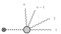
Figure 1: The diagram of the process $\chi\left(p_{\chi}\right)+\mathrm{target}\rightarrow\chi\left(p_{\chi}^{\prime}\right)+\mathrm{target}+\left(\mathbf{k}_{1},\alpha_{1}\right)+\left(\mathbf{k}_{2},\alpha_{2}\right)+\cdots\left(\mathbf{k}_{n},\alpha_{n}\right)$. See text for details.

We consider the scattering process where $n$ phonons $\left\{\mathbf{k}_{j},\alpha_{j}\right\},\,\left(j=1,\,2,\cdots,\,n\right)$ are generated by an incident DM particle in the context of the QFT, where $\left\{\mathbf{k}_{j}\right\}$ and $\left\{\alpha_{j}\right\}$ represent the phonon wavevectors in the first Brillouin zone (1BZ), and phonon polarization branches, of the final states, respectively. The relevant diagram is shown in Fig. 1, where the initial ($\mathbf{p}{}_{\chi}$) and final ($\mathbf{p}^{\prime}{}_{\chi}$) DM states are replaced with an external source. With such replacement it is convenient to switch the scattering theory at zero-temperature to the linear response theory at a finite temperature, where the interest is focused on the response of target material to external perturbations. A more complete treatment of the composite lattice at a finite temperature lies beyond the scope of this work, and will be pursued in further investigation. Using the Feynman rules summarized in Appendix. A.5, the amplitude is read as

$$i\mathcal{M} = \left(-i\right)V_{\chi N}\left(\mathbf{q}\right)N\,\sum_{\mathbf{G}}\delta_{\sum_{j}\mathbf{k}_{j}+\mathbf{q},\,\mathbf{G}}\,e^{-W\left(\mathbf{q}\right)}\prod_{j=1}^{n}\left(\frac{-i\mathbf{q}\cdot\mathbf{\boldsymbol{\epsilon}}_{\mathbf{k}_{j},\alpha_{j}}}{\sqrt{2\,N\,m_{N}\omega_{\mathbf{k}_{j},\alpha_{j}}}}\right),$$ (2.1)

where $\mathbf{q}=\mathbf{p}^{\prime}_{\chi}-\mathbf{p}{}_{\chi}$ is the momentum transferred to the DM particle, $\mathbf{G}$’s are reciprocal lattice vectors, $N$ is the number of the unit cells in the crystal, which equals the number of the atoms in a monatomic simple crystal, $V$ is the volume of the material, $m_{N}$ is the nucleus mass, $\boldsymbol{\epsilon}_{\mathbf{k}_{j},\alpha_{j}}$ and $\omega_{\mathbf{k}_{j},\alpha_{j}}$ are the phonon eigenvector and the eigenfrequency of branch $\alpha_{j}$ at wavevector $\mathbf{k}_{j}$, respectively; $V_{\chi N}\left(\mathbf{q}\right)$ represents the DM-nucleus contact interaction $V_{\chi N}\left(\mathbf{x}\right)$ in momentum space, which connects to the DM-nucleon cross section $\sigma_{\chi n}$ through

$$\left|V_{\chi N}\left(\mathbf{q}\right)\right|^{2} = \left|\int\mathrm{d}^{3}x\,e^{-i\mathrm{\mathbf{q}\cdot\mathbf{x}}}\,V_{\chi N}\left(\mathbf{x}\right)\right|^{2}$$ (2.2)

$$= \frac{A^{2}\pi\sigma_{\chi n}}{\mu_{\chi n}^{2}},$$

with $A$ being the atomic number of the target nucleus, and $\mu_{\chi n}=m_{n}\,m_{\chi}/\left(m_{n}+m_{\chi}\right)$ representing the reduced mass of the DM ($\chi$)-nucleon ($n$) pair system. $W\left(\mathbf{q}\right)=\sum_{\mathbf{k},\alpha}\frac{\left|\mathbf{q}\cdot\mathbf{\boldsymbol{\epsilon}}_{\mathbf{k},\alpha}\right|^{2}}{4Nm_{N}\omega_{\mathbf{k},\alpha}}$ is the Debye-Waller factor at zero-temperature. Since the lattice is not perfectly rigid, the Debye-Waller factor accounts for the effect of the quantum and thermal uncertainties of the positions of the nuclei in the scattering. At $T=0\,\mathrm{K}$, only the zero-point fluctuation is relevant. Thus, the total cross section of the DM-target scattering is expressed as

$$\sigma = \frac{2\pi}{V}N^{2}\sum_{\mathbf{q}}\frac{\left|V_{\chi N}\left(\mathbf{q}\right)\right|^{2}}{v}\sum_{\left\{\mathbf{k}_{j},\alpha_{j}\right\}}\frac{1}{n!}\prod_{j=1}^{n}\left(\frac{\left|\mathbf{q}\cdot\mathbf{\boldsymbol{\epsilon}}_{\mathbf{k}_{j},\alpha_{j}}\right|^{2}}{2\,N\,m_{N}\omega_{\mathbf{k}_{j},\alpha_{j}}}\right)e^{-2W\left(\mathbf{q}\right)}\,\sum_{\mathbf{G}}\delta_{\sum_{j}\mathbf{k}_{j}+\mathbf{q},\,\mathbf{G}}\,\delta\left(\sum_{j=1}^{n}\omega_{\mathbf{k}_{j},\alpha_{j}}+\omega_{p^{\prime}p}\right),$$

(2.3)

where $\omega_{p^{\prime}p}=\left|\mathbf{p}^{\prime}_{\chi}\right|^{2}/\left(2m_{\chi}\right)-\left|\mathbf{p}{}_{\chi}\right|^{2}/\left(2m_{\chi}\right)$ is the energy transferred to the DM particle, and $v$ is its incident velocity. Note that the sum $\sum_{\left\{\mathbf{k}_{j},\alpha_{j}\right\}}$ runs over all possible phonon vibration modes as the final states. In the above expression, the integration of the out-going DM momentum $\mathbf{p}^{\prime}_{\chi}$ is traded for that over the transferred momentum $\mathbf{q}$. Since there are $n$ identical phonons in a final state, the integration over momenta is divided by $n!$. A convenient correspondence $\sum_{\mathbf{G},\mathbf{G}^{\prime}}\delta_{\sum_{j}\mathbf{k}_{j}+\mathbf{q},\,\mathbf{G}}\delta_{\sum_{j}\mathbf{k}_{j}+\mathbf{q},\,\mathbf{G}^{\prime}}$$\sim\sum_{\mathbf{G},\mathbf{G}^{\prime}}\delta_{\sum_{j}\mathbf{k}_{j}+\mathbf{q},\,\mathbf{G}}\delta_{\mathbf{G}\,\mathbf{G}^{\prime}}$$\sim\sum_{\mathbf{G}}\delta_{\sum_{j}\mathbf{k}_{j}+\mathbf{q},\,\mathbf{G}}$ is adopted in evaluating the amplitude squared. A detailed discussion on the quantization of vibrations in solids using the path integral approach is arranged in Appendix. A.

Moreover, note that the momentum $\mathbf{q}$ can be uniquely separated into certain reciprocal lattice $\mathbf{G}_{\mathbf{q}}$, and a remainder part $\left[\mathbf{q}\right]$ within the 1BZ, such that $\mathbf{q}=\mathbf{G}_{\mathbf{q}}+\left[\mathbf{q}\right]$, and thus the summation over $\mathbf{q}$ can be equivalently expressed as the sum $\sum_{\mathbf{G}_{\mathbf{q}}}\sum_{\left[\mathbf{q}\right]\in 1\mathrm{BZ}}$. The integration over $\left[\mathbf{q}\right]$ can always be integrated out from the sum $\sum_{\mathbf{G}}\delta_{\sum_{j}\mathbf{k}_{j}+\mathbf{q},\,\mathbf{G}}$ for an arbitrary set of $\left\{\mathbf{k}_{j}\right\}$ without noticeably affecting the values of other integrand functions $\left(\cdots\right)_{\mathbf{q}}$ that are coarsely dependent on $\mathbf{q}$. The variation of the integrand over the 1BZ is expected to be irrelevant as long as the momentum transfer $q=\left|\mathbf{q}\right|$ is much larger than the length of the 1BZ, i.e., $q\gg\mathcal{O}\left(1\right)\,\mathrm{keV}$. In this case, one has the following incoherent scattering approximation,

$$\sum_{\mathbf{q}}\left(\cdots\right)_{\mathbf{q}}\sum_{\mathbf{G}}\delta_{\sum_{i}\mathbf{k}_{i}+\mathbf{q},\,\mathbf{G}} = \sum_{\mathbf{G}_{\mathbf{q}}}\sum_{\left[\mathbf{q}\right]\in 1\mathrm{BZ}}\left(\cdots\right)_{\mathbf{G}_{\mathbf{q}}+\left[\mathbf{q}\right]}\sum_{\mathbf{G}}\delta_{\sum_{i}\mathbf{k}_{i}+\left[\mathbf{q}\right],\,\mathbf{G}}$$ (2.4)

$$= \sum_{\mathbf{G}_{\mathbf{q}}}\left(\cdots\right)_{\mathbf{G}_{\mathbf{q}}+\mathbf{k}_{0}}$$

$$\simeq \frac{1}{N}\sum_{\mathbf{q}}\left(\cdots\right)_{\mathbf{q}},$$

where a unique $\mathbf{k}_{0}\in 1\mathrm{BZ}$ satisfies $\sum_{\mathbf{G}}\delta_{\sum_{i}\mathbf{k}_{i}+\mathbf{k}_{0},\,\mathbf{G}}=1$. This approximation amounts to smoothing out $\mathbf{q}$ within the 1BZ as if one can only see a momentum transfer with a resolution comparable to the length of a reciprocal lattice. Next, we further approximate that the simple lattice is isotropic. In this case, eigenenergy $\omega_{\mathbf{k},\alpha}$ remains invariant under any rotational operation $\mathcal{O}_{R}$ acting on wavevector $\mathbf{k}$, while $\mathbf{\boldsymbol{\epsilon}}_{\mathbf{k},\alpha}$ also transforms as a vector under the same $\mathcal{O}_{R}$, and thus one has

$$\sum_{\mathbf{k},\alpha}\frac{\left|\mathbf{q}\cdot\mathbf{\boldsymbol{\epsilon}}_{\mathbf{k},\alpha}\right|^{2}}{2Nm_{N}\omega_{\mathbf{k},\alpha}} = E_{R}\left(q\right)\sum_{i=1}^{3N}\frac{1}{3N}\frac{1}{\omega_{i}},$$ (2.5)

where $E_{R}\left(q\right)=q^{2}/\left(2m_{N}\right)$. This result also holds for a monatomic cubic system [62]. In the right-hand-side of Eq. (2.5), we relabel the eigenmodes $\left\{\mathbf{k},\alpha\right\}$ with a single notation $\left\{i\right\}$ for brevity, and Eq. (2.3) in the incoherent approximation is recast as

$$\sigma \simeq \frac{2\pi}{V}N\sum_{\mathbf{q}}\frac{\left|V_{\chi N}\left(\mathbf{q}\right)\right|^{2}}{v}\times S\left(q,\,-\omega_{p^{\prime}p}\right)$$ (2.6)

$$= \frac{2\pi}{V}\sum_{\mathbf{q}}N\frac{\left|V_{\chi N}\left(\mathbf{q}\right)\right|^{2}}{v}$$

$$\times\sum_{\left\{n_{i}\right\}}\frac{e^{-\frac{E_{R}\left(q\right)}{3N\omega_{1}}}}{n_{1}!}\left(\frac{E_{R}\left(q\right)}{3N\omega_{1}}\right)^{n_{1}}\cdots\frac{e^{-\frac{E_{R}\left(q\right)}{3N\omega_{3N}}}}{n_{3N}!}\left(\frac{E_{R}\left(q\right)}{3N\omega_{3N}}\right)^{n_{3N}}\delta\left(\sum_{i=1}^{3N}n_{i}\omega_{i}+\omega_{p^{\prime}p}\right)$$

$$= \frac{2\pi}{V}\sum_{\mathbf{q}}N\frac{\left|V_{\chi N}\left(\mathbf{q}\right)\right|^{2}}{v}\times e^{-E_{R}\left(q\right)\sum_{i=1}^{3N}\frac{1}{3N}\frac{1}{\omega_{i}}}\sum_{n=0}^{+\infty}\frac{E_{R}\left(q\right)^{n}}{n!}T_{n}\left(-\omega_{p^{\prime}p}\right),$$

where the scattering function $S\left(q,\,-\omega_{p^{\prime}p}\right)$ is defined in the third line, $n_{i}$ represents the occupation number of the energy $\omega_{i}$, and $\overline{\omega}=\sum_{i=1}^{3N}\frac{\omega_{i}}{3N}$ is the phonon frequency averaged over the density of states (DoS). Note that $\sum_{\left\{n_{i}\right\}}\frac{e^{-\frac{E_{R}\left(q\right)}{3N\omega_{1}}}}{n_{1}!}\left(\frac{E_{R}\left(q\right)}{3N\omega_{1}}\right)^{n_{1}}\cdots\frac{e^{-\frac{E_{R}\left(q\right)}{3N\omega_{3N}}}}{n_{3N}!}\left(\frac{E_{R}\left(q\right)}{3N\omega_{3N}}\right)^{n_{3N}}$ is a combined Poisson distribution, so the key problem is to determine the probability density of the random variable $\omega=\sum_{i=1}^{3N}n_{i}\omega_{i}$ for this distribution. While it is difficult to derive an analytical expression on a general basis, one can prove that the factor $S\left(q,\,\omega\right)$ converges to a Gaussian form in the large $q$ region, i.e., $e^{-\frac{\left(\omega-E_{R}\left(q\right)\right)^{2}}{2E_{R}\left(q\right)\overline{\omega}}}/\sqrt{2\pi E_{R}\left(q\right)\overline{\omega}}$, by using an argument analogous to that used in the proof of the central limit theorem. Additionally, this Gaussian form converges to the delta function in terms of the energy conservation towards the large $q$ limit, which validates the impulse approximation. In the large $q$ regime, the scattering function $S\left(q,\,\omega\right)$ can be approximated with an asymptotic expansion with respect to parameter $\sqrt{\overline{\omega}/E_{R}\left(q\right)}$ as follows (see Appendix A.8 for a detailed discussion),

$$S\left(q,\,\omega\right) = \frac{e^{-\frac{\left(\omega-E_{R}\left(q\right)\right)^{2}}{2E_{R}\left(q\right)\overline{\omega}}}}{\sqrt{2\pi E_{R}\left(q\right)\overline{\omega}}}\left\{1+\frac{1}{6}\left(\frac{\overline{\omega^{2}}}{\overline{\omega}^{2}}\right)\cdot\left[\frac{\left(\omega-E_{R}\left(q\right)\right)^{2}}{E_{R}\left(q\right)\overline{\omega}}-3\right]\cdot\frac{\left(\omega-E_{R}\left(q\right)\right)}{\sqrt{E_{R}\left(q\right)\overline{\omega}}}\cdot\sqrt{\frac{\overline{\omega}}{E_{R}\left(q\right)}}\right\}+o\left(\sqrt{\frac{\overline{\omega}}{E_{R}\left(q\right)}}\right),$$

with $\overline{\omega^{2}}=\sum_{i=1}^{3N}\frac{1}{3N}\omega_{i}^{2}$. To get some sense, taking silicon target for example, in the top row of Fig. 2 we show the non-dimensional function $\overline{\omega}S\left(q,\,\omega\right)$ for parameters $\sqrt{E_{R}\left(q\right)/\overline{\omega}}=5$ and $10$, respectively. It is evident that in the regime $\sqrt{E_{R}\left(q\right)/\overline{\omega}}\gtrsim 5$, the compound Poisson distribution in the third line of Eq. (2.6) already well resembles the asymptotic Gaussian form in shape, except for a minor displacement of the central value $E_{R}\left(q\right)$.

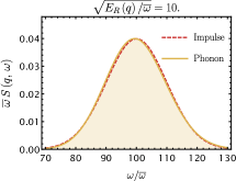
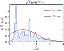
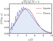
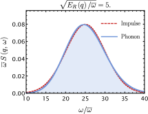
Figure 2: Top: Comparisons between the function $\overline{\omega}S\left(q,\,\omega\right)$ of silicon for the multi-phonon distribution (orange) and the impulse Gaussian (red dashed curves) for the ratios $\sqrt{E_{R}\left(q\right)/\overline{\omega}}=5$ and $10$, respectively. The multi-phonon distributions are estimated with the asymptotic expansion (up to $\mathcal{O}\left(\sqrt{\overline{\omega}/E_{R}\left(q\right)}\right)$) presented in Eq. (LABEL:eq:Asymptotic). Bottom: Comparisons between the function $\overline{\omega}S\left(q,\,\omega\right)$ of silicon for the multi-phonon distribution (blue histograms) obtained by the numerical recursive method and the impulse Gaussian (red dashed curves) for the ratios $\sqrt{E_{R}\left(q\right)/\overline{\omega}}=1,\,2,$ and $5$, respectively. Similar discussion can be found in Ref. [50]. See text for details.

For a small transferred momentum $q$, the asymptotic expansion above is no longer valid. In this case, one can alternatively utilize the functions $\left\{T_{n}\left(\omega\right)\right\}$ in the last line of Eq. (2.6) so as to calculate the scattering function $S\left(q,\,\omega\right)$ in a numerical fashion. Defined as

$$T_{n}\left(\omega\right) = \frac{1}{2\pi}\int_{-\infty}^{+\infty}f\left(t\right)^{n}e^{-i\omega t}\mathrm{d}t,$$ (2.8)

where

$$f\left(t\right) = \sum_{i=1}^{3N}\frac{1}{3N}\frac{e^{i\omega_{i}t}}{\omega_{i}},$$ (2.9)

these $\left\{T_{n}\left(\omega\right)\right\}$ can be determined by following an iterative procedure (see Appendix A.9 for further details):

$$\int_{-\infty}^{+\infty}T_{1}\left(\omega-\omega^{\prime}\right)T_{n-1}\left(\omega^{\prime}\right)\mathrm{d}\omega^{\prime} = T_{n}\left(\omega\right).$$ (2.10)

In the bottom row of Fig. 2 we present the non-dimensional function $\overline{\omega}S\left(q,\,\omega\right)$ of silicon target computed with recursive method for parameters $\sqrt{E_{R}\left(q\right)/\overline{\omega}}=1,\,2,$ and $5$, respectively. It illustrates the transition from the multi-phonon spectrum into a Gaussion form with an increasing momentum transfer $q$. Taking typical semiconductors such as silicon for instance, where $\overline{\omega}=40.3\,\mathrm{meV}$, the condition $\sqrt{E_{R}\left(q\right)/\overline{\omega}}\gtrsim 1$ translates to a momentum transfer $q\gtrsim\mathcal{O}\left(10\right)\,\mathrm{keV},$ which still guarantees the validity of the incoherent approximation. In the limit $q\rightarrow\infty$, the width of the Gaussian becomes much smaller than the central value $E_{R}\left(q\right)$, and hence the Gaussian reduces to the $\delta$-function $\delta$$\left(\omega_{p^{\prime}p}+E_{R}\left(q\right)\right)$. Then inserting Eq. (2.2), and taking the correspondence $\sum_{\mathbf{q}}\sim\frac{V}{\left(2\pi\right)^{3}}\int\mathrm{d^{3}}q$, the cross section in the limit $q\rightarrow\infty$ becomes

$$\sigma = \frac{A^{2}\pi\sigma_{\chi n}N}{\mu_{\chi n}^{2}v}\int\frac{\mathrm{d^{3}}q}{\left(2\pi\right)^{2}}\,\delta\left(\frac{q^{2}}{2\mu_{\chi N}}+\mathbf{q}\cdot\mathbf{v}\right),$$ (2.11)

which, as expected, is equal to the sum of $N$ incoherent DM-nucleus cross sections for monatomic simple crystal structure.

3 Migdal effect as a multi-phonon process

The prospect of describing the Migdal effect in terms of phonons and electrons has been originally sketched out in Ref. [51]. Here we explore this approach in more details. The Migdal excitation process is illustrated in Fig. 3, where an electron-hole pair is excited through a virtual phonon, along with a bunch of on-shell ones produced from the collision with a DM particle. In essence, the electron-phonon interaction reflects the Coulomb forces between the distorted ion lattice and the itinerant electrons, for which we provide a short review in Appendix. A.4.

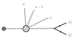
Figure 3: The diagram for the Migdal effect, where an electron-hole pair is generated, i.e., an electron is elevated from a valence state $\ket{j}$ to a conduction state $\ket{i}$, via the exchange of a virtual phonon, along with multiple on-shell phonons generated by the DM external field.

Following the Feynman rules summarized in Sec. A.5, one can read off the amplitude for the process illustrated in Fig. 3,

$$i\mathcal{M} = \left(-i\right)V_{\chi N}\left(\mathbf{q}\right)N\,e^{-W\left(\mathbf{q}\right)}\,\prod_{s=1}^{n}\left(\frac{-i\mathbf{q}\cdot\mathbf{\boldsymbol{\epsilon}}_{\mathbf{k}_{s},\alpha_{s}}}{\sqrt{2\,N\,m_{N}\omega_{\mathbf{k}_{s},\alpha_{s}}}}\right)$$ (3.12)

$$\times\sum_{\mathbf{G}^{\prime}}\sum_{\mathbf{k},\alpha}\left(\frac{-i\mathbf{q}\cdot\mathbf{\boldsymbol{\epsilon}}_{\mathbf{k},\alpha}}{\sqrt{Nm_{N}}}\right)\left[\frac{i}{\left(\varepsilon_{i}-\varepsilon_{j}\right)^{2}-\omega_{\mathbf{k},\alpha}^{2}}\right]\left[\frac{i\,\left(\mathbf{k}+\mathbf{G}^{\prime}\right)\cdot\mathbf{\boldsymbol{\epsilon}}_{\mathbf{k},\alpha}}{\sqrt{Nm_{N}}}\right]\left[\frac{-iNZ_{\mathrm{ion}}4\pi\alpha_{e}}{V\left|\mathbf{k}+\mathbf{G}^{\prime}\right|^{2}}\right]\braket{i}{e^{i\left(\mathbf{k}+\mathbf{G}^{\prime}\right)\cdot\hat{\mathbf{x}}}}{j}$$

$$\times\sum_{\mathbf{G}}\delta_{\sum_{s}\mathbf{k}_{s}+\mathbf{q}+\mathbf{k},\,\mathbf{G}},$$

where $Z_{\mathrm{ion}}$ is the number of the valence electrons of the material atom, $\alpha_{e}$ is the fine structure constant, and $\varepsilon_{i}$ ($\varepsilon_{j}$) denotes the energy of the conduction (valence) state $\ket{i}$ ($\ket{j}$). The $n$-phonon sector in the first line has been thoroughly discussed in the preceding section. In the second line lies a phonon mediator with its two ends linking the multi-phonon blob and the bare phonon-electron vertex. For typical semiconductors, the band gaps $\varepsilon_{g}\sim\mathcal{O}\left(1\right)\mathrm{eV}$ are much larger than the phonon eigenenergies $\omega_{\mathbf{k},\alpha}\sim\mathcal{O}\left(10^{-2}\right)\mathrm{eV}$, so the term in second line can be reduced to

$$\frac{Z_{\mathrm{ion}}}{\left(\varepsilon_{i}-\varepsilon_{j}\right)^{2}}\,\sum_{\mathbf{G}^{\prime}}\sum_{\mathbf{k}}\left[\frac{\mathbf{q}\cdot\left(\mathbf{k}+\mathbf{G}^{\prime}\right)}{m_{N}}\right]\left[\frac{4\pi\alpha_{e}}{V\left|\mathbf{k}+\mathbf{G}^{\prime}\right|^{2}}\right]\braket{i}{e^{i\left(\mathbf{k}+\mathbf{G}^{\prime}\right)\cdot\hat{\mathbf{x}}}}{j}.$$ (3.13)

In the derivation, we use the contraction relation $\sum_{\alpha}\left(\mathbf{q}\cdot\mathbf{\boldsymbol{\epsilon}}_{\mathbf{k},\alpha}\right)\left[\left(\mathbf{k}+\mathbf{G}^{\prime}\right)\cdot\mathbf{\boldsymbol{\epsilon}}_{\mathbf{k},\alpha}\right]=\mathbf{q}\cdot\left(\mathbf{k}+\mathbf{G}^{\prime}\right)$. Recall that in Refs. [50, 51] the same amplitude is obtained in the the soft limit, i.e., $\mathbf{p}_{N}\cdot\left(\mathbf{k}+\mathbf{G}\right)/m_{N}\ll\varepsilon_{i}-\varepsilon_{j}$ and $\left|\mathbf{k}+\mathbf{G}\right|\ll\left|\mathbf{p}_{N}\right|$, with $\mathbf{p}_{N}$ being the momentum of the recoiling nucleus. In the low-energy regime however, neither the soft approximation nor the concept of a freely-recoiling nucleus still holds. In contrast, in the context of electrons and phonons, this particular form of amplitude naturally extends to the low-energy regime. The excitation rate (in the incoherent approximation) can then be written as

$$R = \frac{\rho_{\chi}}{m_{\chi}}\int\mathrm{d^{3}}v\,\sigma\,vf_{\chi}\left(\mathbf{v}\right)$$ (3.14)

$$= \frac{\rho_{\chi}}{m_{\chi}}\frac{2\pi A^{2}\sigma_{\chi n}\,Z_{\mathrm{ion}}^{2}\,N_{T}}{V^{2}\mu_{\chi n}^{2}}\int\frac{\mathrm{d}\omega}{\omega^{4}}\,\int\mathrm{d^{3}}v\,f_{\chi}\left(\mathbf{v}\right)\sum_{\mathbf{q}}\,e^{-E_{R}\left(q\right)\sum_{k}\frac{1}{3N}\frac{1}{\omega_{k}}}\,\sum_{n=0}^{+\infty}\frac{E_{R}\left(q\right)^{n}}{n!}T_{n}\left(-\mathbf{v}\cdot\mathbf{q}-\frac{q^{2}}{2m_{\chi}}-\omega\right)$$

$$\times\sum_{\mathbf{G},\mathbf{G}^{\prime}}\sum_{\mathbf{k}\in 1\mathrm{BZ}}\left[\frac{\mathbf{q}\cdot\left(\mathbf{k}+\mathbf{G}\right)}{m_{N}}\right]\left[\frac{\mathbf{q}\cdot\left(\mathbf{k}+\mathbf{G}^{\prime}\right)}{m_{N}}\right]\frac{4\pi\alpha_{e}}{\left|\mathbf{\mathbf{k}}+\mathbf{G}\right|\left|\mathbf{\mathbf{k}}+\mathbf{G}^{\prime}\right|}$$

$$\times\frac{2}{V}\frac{4\pi^{2}\alpha_{e}}{\left|\mathbf{\mathbf{k}}+\mathbf{G}\right|\left|\mathbf{\mathbf{k}}+\mathbf{G}^{\prime}\right|}\sum_{i,j}\braket{i}{e^{i\left(\mathbf{\mathbf{\mathbf{\mathbf{k}}+\mathbf{G}}}^{\prime}\right)\cdot\hat{\mathbf{x}}}}{j}\braket{j}{e^{-i\left(\mathbf{\mathbf{\mathbf{\mathbf{k}}+\mathbf{G}}}\right)\cdot\hat{\mathbf{x}}}}{i}\delta\left(\varepsilon_{i}-\varepsilon_{j}-\omega\right),$$

where $\rho_{\chi}$ represents the DM local density, $f_{\chi}\left(\mathbf{v}\right)$ is the DM velocity distribution. Note that the number of the nuclei $N$ in solids, which equals the number of the primitive cells for a simple lattice structure, is explicitly represented with $N_{T}$ here. The factor $2$ in the last line counts the two spin orientations for each valence state. For the present we have not taken into account the renormalization effect in our discussion, which can displace the locations of the phonon poles, and induce the screening of the Coulomb interaction. Since the band gaps are far larger than the phonon eigenenergies, only the screening effect that leads to a reduction of the scattering rate is relevant for our discussion.

Here we take the homogeneous electron gas (HEG) for a schematic illustration. As shown in Appendix. A.7 and explained in Ref. [51, 50, 66], the screening of the electron-phonon vertex adds an inverse dielectric function $\epsilon^{-1}\left(\mathbf{k},\,\omega\right)$ to the amplitude analogous to Eq. (3.12) of a crystal structure, while the last line in Eq. (3.14) corresponds to $\mathrm{Im}\left[\epsilon\left(\mathbf{k},\,\omega\right)\right]$ at the random phase approximation (RPA) level. Therefore, the overall screening effect is encoded in the energy loss function (ELF) $\mathrm{Im}\left[-\epsilon^{-1}\left(\mathbf{k},\,\omega\right)\right]=\mathrm{Im}\left[\epsilon\left(\mathbf{k},\,\omega\right)\right]/\left|\epsilon\left(\mathbf{k},\,\omega\right)\right|^{2}$, which right approaches the last line in Eq. (3.14) in the limit $\alpha_{e}\rightarrow 0$, as the screening effect becomes negligible. Using the substitution $\sum_{\mathbf{q}}\sim\frac{V}{\left(2\pi\right)^{3}}\int\mathrm{d^{3}}q$ and $\sum_{\mathbf{k}}\sim\frac{V}{\left(2\pi\right)^{3}}\int_{1\mathrm{BZ}}\mathrm{d^{3}}k$, the above event rate can be recast as

$$R = \frac{\rho_{\chi}}{m_{\chi}}\frac{2\,\alpha_{e}A^{2}\sigma_{\chi n}\,Z_{\mathrm{ion}}^{2}\,N_{T}}{3\,\Omega\,\mu_{\chi n}^{2}\,m_{N}^{2}}\,\int\mathrm{d^{3}}v\,\frac{f_{\chi}\left(\mathbf{v}\right)}{v}\int\frac{\mathrm{d}\omega}{\omega^{4}}\,\mathcal{F}\left(\omega\right)\,\int q^{3}\,\mathrm{d}q\,e^{-E_{R}\left(q\right)\sum_{i}\frac{1}{3N}\frac{1}{\omega_{i}}}\,\sum_{n=0}^{+\infty}\frac{E_{R}\left(q\right)^{n}}{n!}\int_{0}^{qv-\frac{q^{2}}{2m_{\chi}}-\omega}T_{n}\left(E\right)\mathrm{d}E,$$

where the nondimensional factor

$$\mathcal{F}\left(\omega\right) = \sum_{\mathbf{G},\mathbf{G}^{\prime}}\int_{1\mathrm{BZ}}\frac{\varOmega\,\mathrm{d}^{3}k}{\left(2\pi\right)^{3}}\,\frac{\left(\mathbf{k}+\mathbf{G}\right)\cdot\left(\mathbf{k}+\mathbf{G}^{\prime}\right)}{\left|\mathbf{k}+\mathbf{G}\right|\left|\mathbf{k}+\mathbf{G}^{\prime}\right|}\,\mathrm{Im}\left[-\widetilde{\epsilon}_{\mathbf{G},\mathbf{G}^{\prime}}^{-1}\left(\mathbf{k},\omega\right)\right]$$ (3.16)

represents the averaged energy loss function, with $\Omega$ being the volume of the unit cell, and $\mathrm{Im}\left[\tilde{\epsilon}_{\mathbf{G},\mathbf{G}^{\prime}}^{-1}\left(\mathbf{\mathbf{\mathbf{k}}},\omega\right)\right]$ (see Appendix A.6) being the EFL for the crystal structure. $\mathcal{F}\left(\omega\right)$ has been calculated for diamond and silicon targets in Ref. [51]. Eq. (LABEL:eq:eventRate-1) applies for the crystal targets that can be considered as isotropic, in which case only the one-dimensional DM speed distribution is relevant for the calculation of the excitation rate in Eq. (3.14), and thus an isotropic velocity distribution $f_{\chi}\left(\mathbf{v}\right)$ is assumed. In the derivation, we first integrate out the angular variable of velocity $\mathbf{v}$ with respect to $\mathbf{q}$, which converts to the integral over variable $E$ in Eq. (LABEL:eq:eventRate-1), and restore the full integration over velocity distribution (by adding a factor $1/2$) for convenience. Then we integrate out the solid angle of momentum transfer $\mathbf{q}$ using the Legendre addition theorem, which leads to the factor $\mathcal{F}\left(\omega\right)$.

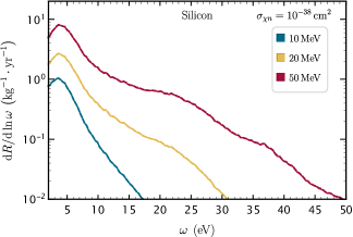
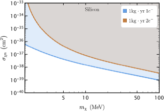
Figure 4: Left: The differential Migdal electronic excitation event rates in bulk silicon for a reference cross section $\sigma_{\chi n}=10^{-38}\,\mathrm{cm}^{2}$ and DM masses $m_{\chi}=10\,\mathrm{MeV}$ (emerald), $20\,\mathrm{MeV}$(orange) and $50\,\mathrm{MeV}$ (maroon), respectively; the solid lines and the dashed lines are calculated using the phonon-mediated approach and the bremsstrahlung-like approach, respectively. The results from the two approaches coincide so well that they can hardly be distinguished in the plot. Right: Sensitivities for the Migdal effect at 90% C.L. for a 1 kg$\cdot$yr silicon detector, based on the single-electron (blue) and the two-electron (orange) ionization signal bins. The upper limits calculated using the phonon-mediated approach (solid) and the bremsstrahlung-like approach (dashed) coincide throughout the whole DM mass range. See text for details.

It is interesting to compare the event rate Eq. (LABEL:eq:eventRate-1) with the one derived in the picture of the bremsstrahlung-like process proposed in Ref. [51], which is expressed as

$$R = \frac{\rho_{\chi}}{m_{\chi}}\frac{2\,\alpha_{e}A^{2}\sigma_{\chi n}\,Z_{\mathrm{ion}}^{2}\,N_{T}}{3\,\Omega\,\mu_{\chi n}^{2}\,m_{N}^{2}}\,\int\mathrm{d^{3}}v\,\frac{f_{\chi}\left(\mathbf{v}\right)}{v}\int\frac{\mathrm{d}\omega}{\omega^{4}}\,\mathcal{F}\left(\omega\right)\,\int p{}_{N}^{3}\,\mathrm{d}p_{N}\times\varTheta\left[p_{N}v-\frac{p_{N}^{2}}{2\,\mu_{\chi N}}-\omega\right],$$ (3.17)

with $p_{N}$ and $\mu_{\chi N}=m_{N}\,m_{\chi}/\left(m_{N}+m_{\chi}\right)$ being momentum of the recoiled nucleus and the reduced mass of the DM-nucleus pair, respectively. $\varTheta$ is the Heaviside step function. In the sub-GeV mass regime, $\mu_{\chi N}\approx m_{\chi}$. Since the integrand functions $\left\{T_{n}\left(E\right)\right\}$ vanish if $E<0$, we set the lower limit of the integral to be $0$ in Eq. (LABEL:eq:eventRate-1) for convenience. But note that $T_{0}\left(E\right)=\delta\left(E\right)$ also contributes to the event rate if $E>0$ in Eq. (LABEL:eq:eventRate-1), which corresponds to the process where an electron-hole pair is excited without generating any phonons.

In our computations, we take $\rho_{\chi}=0.3\,\mathrm{GeV/cm^{3}}$, and the velocity distribution is approximated as a truncated Maxwellian form in the Galactic rest frame, i.e., $f_{\chi}\left(\mathbf{v}\right)\propto\exp\left[-\left|\mathbf{v}+\mathbf{v}_{\mathrm{e}}\right|^{2}/v_{0}^{2}\right]\,\Theta\left(v_{\mathrm{esc}}-\left|\mathbf{v}+\mathbf{v}_{\mathrm{e}}\right|\right)$, with the Earth’s velocity $v_{\mathrm{e}}=230\,\mathrm{km/s}$, the dispersion velocity $v_{0}=220\,\mathrm{km/s}$ and the Galactic escape velocity $v_{\mathrm{esc}}=544\,\,\mathrm{km/s}$ [67]. In the left panel of Fig. 4 shown is the comparison between the Migdal event rates in silicon semiconductor target calculated with the phonon-mediated approach and the bremsstrahlung-like method, for DM masses $m_{\chi}=10\,\mathrm{MeV}$, $20\,\mathrm{MeV}$ and $50\,\mathrm{MeV}$, respectively, for a benchmark cross section $\sigma_{\chi n}=10^{-38}\,\mathrm{cm}^{2}$. It is observed that even in the small DM mass range ($m_{\chi}<50\,\mathrm{MeV}$), where the impulse approximation is no longer expected to be reliable, the bremsstrahlung-like narrative still well coincides with the result calculated with the phonon-mediated approach. This can be partly understood from a closer observation of $S\left(q,\,E\right)$: for a DM mass below $10\,\mathrm{MeV}$ with a typical momentum transfer $q=m_{\chi}\cdot 10^{-3}$$<10\,\mathrm{keV}$, $S\left(q,\,E\right)$ is dominated by $T_{0}\left(E\right)=\delta\left(E\right)$, and thus $\int^{qv-\frac{q^{2}}{2m_{\chi}}-\omega}S\left(q,\,E\right)\mathrm{d}E\simeq\varTheta\left(qv-\frac{q^{2}}{2m_{\chi}}-\omega\right)$, in consistence with the bremsstrahlung-like expression in Eq. (3.17). For larger DM masses with a typical velocity $10^{-3}\,c$, $S\left(q,\,E\right)$ resembles a Gaussian form centered at $E_{R}=q^{2}/\left(2m_{N}\right)\ll q^{2}/\left(2m_{\chi}\right)\sim\mathcal{O}\left(qv-\frac{q^{2}}{2m_{\chi}}-\omega\right)$, and again one has $\int^{qv-\frac{q^{2}}{2m_{\chi}}-\omega}S\left(q,\,E\right)\mathrm{d}E\simeq\varTheta\left(qv-\frac{q^{2}}{2m_{\chi}}-\omega\right)$. This relation holds as long as the weight of $S\left(q,\,E\right)$ lies below $qv-\frac{q^{2}}{2m_{\chi}}-\omega$.

In the right panel of Fig. 4 we present the expected 90% C.L. sensitivity of silicon target to cross section $\sigma_{\chi n}$ with $1$ kg$\cdot$yr of exposure, based on the phonon-mediated (solid) and bremsstrahlung-like (dashed) approaches, for a single-electron (blue) and a two-electron (orange) charge bins, respectively, under the zero background assumption.

4 Summary and discussion

In this paper we build up a phonon-mediated description of the Migdal effect in semiconductor targets in the context of the solid state QFT, in which the phonons, namely, the quantized collective vibrations of the ions, rather than the on-shell ions, are used to describe the Migdal excitation process.

In order to ease the discussion, three major simplifications of the problem are made: (1) we assume the solid target is a monatomic simple crystal, possessing an approximately rotational symmetry; (2) we use the zero-temperature QFT in formulating the multi-phonon scattering event rates, rather than a more general finite temperature QFT framework; (3) we take the incoherent approximation in calculating the multi-phonon process. While the isotropy approximation in (1) is valid for the diamond structure materials (e.g., silicon and germanium), it may result in uncertainty for some anisotropic materials (e.g., sapphire). The second assumption is sufficient for experiments operated at cryogenic temperatures. In fact, it is straightforward to generalize the zero-temperature formalism to the finite temperature one by simply replacing the propagators of the zero-temperature case in Eq. (3.12) with those in the finite temperature scenario. As for the third approximation, note that for DM masses around an MeV, the typical momentum transfer can be as small as $q\sim\mathcal{O}\left(1\right)\,\mathrm{keV}$, which is comparable to the size of the 1BZ, and hence beyond the regime of validity for the incoherent approximation. Further study for $m_{\chi}<1\,\mathrm{MeV}$ is needed.

Based on the formalism, we numerically calculate the Migdal excitation event rates for the silicon semiconductor target. As expected, the multi-phonon energy spectra are found to well converge to the Gaussian form in the large $q$ limit, justifying the impulse approximation used in the bremsstrahlung-like description. Although the behavior of the phonon scattering function $S\left(q,\omega\right)$ differ from that of a free nucleus in the low and intermediate scattering energy region, the Migdal excitation rates calculated from the impulse approximation are found to be well consistent with that obtained using the phonon-mediated approach throughout the relevant DM mass range. Finally, it is tempting to apply the phonon-mediated approach to the probe of sub-MeV DM particles through the Migdal effect in novel narrow-gap materials with band gaps of $\mathcal{O}\left(10\right)\mathrm{meV}$ (e.g., Dirac materials), where the picture of the free-recoiling nucleus turns invalid altogether. We leave it for the future work.

Note added. After this work was published, Kim Berghaus suggested us that the contribution of $T_{0}$ was omitted in our original numerical implementation of Eq. (LABEL:eq:eventRate-1), which as a consequence can remarkably suppress the calculated event rates for a small $q$ (an upcoming paper [68] also discusses the Migdal effect in semiconductor detectors). After $T_{0}$ term is included, it is found that the Migdal event rates calculated from the phonon-mediated approach and the impulse approximation coincide quite well even in the low DM mass range.

Appendix A Phonons in the quantum field theory

For easy reading, we provide an elementary introduction to relevant theoretical background to the main text in this appendix, including the treatment of the phonons and electrons, as well as their interactions in the context of the QFT. Part of the material can be found in Ref. [69].

A.1 Quantization of vibrations in solids

For simplicity here we only consider the case of the monatomic simple lattices. The dynamics of the crystal vibration is described with the following equation,

$$m_{N}\ddot{\mathbf{u}}_{\boldsymbol{\ell}}+\sum_{\boldsymbol{\ell}^{\prime}}\Phi\left(\boldsymbol{\ell}-\boldsymbol{\ell}^{\prime}\right)\,\mathbf{u}_{\boldsymbol{\ell}^{\prime}} = 0,$$ (A.18)

where $m_{N}$ is the nucleus mass, $\mathbf{u}_{\boldsymbol{\ell}}$ is the displacement of the nucleus at lattice site $\boldsymbol{\ell}$, and the force strength matrix elements are explicitly expressed as follows,

$$\Phi\left(\boldsymbol{\ell}-\boldsymbol{\ell}^{\prime}\right)_{\sigma\sigma^{\prime}} = \left.\frac{\partial^{2}U}{\partial u_{\boldsymbol{\ell}\sigma}\,\partial u_{\boldsymbol{\ell}^{\prime}\sigma^{\prime}}}\right|_{\mathbf{u}=0},$$ (A.19)

with $U$ being the potential between the nuclei at sites $\boldsymbol{\ell}$ and $\boldsymbol{\ell}^{\prime}$, and $\sigma,\,\sigma^{\prime}=\left\{x,\,y,\,z\right\}$ denoting the three space directions. The Fourier transform of the force strength matrix is called the dynamical matrix $V\left(\mathbf{k}\right)$, i.e.,

$$V\left(\mathbf{k}\right) = \sum_{\ell}\Phi\left(\boldsymbol{\ell}\right)e^{-i\mathbf{k}\cdot\boldsymbol{\ell}},$$ (A.20)

which is real symmetric matrix for the Bravais lattice at each wave-vector $\mathbf{k}$ in the 1BZ, and thus can be diagonalized with an orthonormal basis set of vectors $\left\{\mathbf{\boldsymbol{\epsilon}}_{\mathbf{k},1},\,\mathbf{\boldsymbol{\epsilon}}_{\mathbf{k},2},\,\mathbf{\boldsymbol{\epsilon}}_{\mathbf{k},3}\right\}$, such that

$$\mathbf{\boldsymbol{\epsilon}}_{\mathbf{k},\alpha}\cdot\mathbf{\boldsymbol{\epsilon}}_{\mathbf{k},\alpha^{\prime}} = \delta_{\alpha,\alpha^{\prime}}.$$ (A.21)

and

$$\mathbf{\boldsymbol{\epsilon}}_{\mathbf{k},\alpha^{\prime}}^{T}V\left(\mathbf{k}\right)\mathbf{\boldsymbol{\epsilon}}_{\mathbf{k},\alpha^{\prime}} = \omega_{\mathbf{k},\alpha}^{2}\delta_{\alpha,\alpha^{\prime}},$$ (A.22)

with $\omega\left(\mathbf{k},\alpha\right)$ being corresponding eigenfrequency of the mode $\left(\mathbf{k},\,\alpha\right)$. Besides, since $\Phi\left(\boldsymbol{\ell}\right)=\Phi\left(-\boldsymbol{\ell}\right)$ for Bravais lattice, it is straightforward to see that $V\left(\mathbf{k}\right)=V\left(-\mathbf{k}\right)$, $\mathbf{\boldsymbol{\epsilon}}_{\mathbf{k},\alpha}=\mathbf{\boldsymbol{\epsilon}}_{-\mathbf{k},\alpha}$ and $\omega_{\mathbf{k},\alpha}=\omega_{-\mathbf{k},\alpha}$. With these preparations, one first substitutes the displacements with eigen-vibration modes:

$$\mathbf{u}_{\boldsymbol{\ell}} = \sum_{\mathbf{k}\in 1\mathrm{BZ}}\,\sum_{\alpha=1}^{3}\frac{\mathbf{\boldsymbol{\epsilon}}_{\mathbf{k},\alpha}\,e^{i\mathbf{k}\cdot\boldsymbol{\ell}}}{\sqrt{N\,m_{N}}}\,Q_{\mathbf{k},\alpha},$$ (A.23)

where $Q_{\mathbf{k},\alpha}$ encodes the vibration amplitude for the mode $\left(\mathbf{k},\,\alpha\right)$, and $N$ is the number of the unit cells in the material, and then obtains the Lagrangian of vibration system,

$$L = \frac{1}{2}\left(\sum_{\boldsymbol{\ell}}m_{N}\,\mathbf{\dot{u}}_{\boldsymbol{\ell}}\cdot\mathbf{\dot{u}}_{\boldsymbol{\ell}}-\sum_{\boldsymbol{\ell},\boldsymbol{\ell}^{\prime}}\mathbf{u}_{\boldsymbol{\ell}}^{T}\,\Phi\left(\boldsymbol{\ell}-\boldsymbol{\ell}^{\prime}\right)\mathbf{u}_{\boldsymbol{\ell}^{\prime}}\right)$$ (A.24)

$$= \frac{1}{2}\sum_{\mathbf{k},\alpha}\left(\dot{Q}_{-\mathbf{k},\alpha}\,\dot{Q}_{\mathbf{k},\alpha}-\omega_{\mathbf{k},\alpha}^{2}Q_{-\mathbf{k},\alpha}\,Q_{\mathbf{k},\alpha}\right),$$

and the equations of motion

$$\ddot{Q}_{\mathbf{k},\alpha}+\omega_{\mathbf{k},\alpha}^{2}Q_{\mathbf{k},\alpha} = 0.$$ (A.25)

One then follows the conventional quantization procedures to give pairs of the canonical position and momentum operators

$$\hat{Q}_{\mathbf{k},\alpha}\left(t\right) = \frac{1}{\sqrt{2\,\omega_{\mathbf{k},\alpha}}}\left(\hat{a}_{\mathbf{k},\alpha}e^{-i\omega_{\mathbf{k},\alpha}t}+\hat{a}_{-\mathbf{k},\alpha}^{\dagger}e^{i\omega_{\mathbf{k},\alpha}t}\right),$$

$$\hat{P}_{\mathbf{k},\alpha}\left(t\right) = -i\sqrt{\frac{\omega_{\mathbf{k},\alpha}}{2}}\left(\hat{a}_{-\mathbf{k},\alpha}e^{-i\omega_{\mathbf{k},\alpha}t}-\hat{a}_{\mathbf{k},\alpha}^{\dagger}e^{i\omega_{\mathbf{k},\alpha}t}\right),$$ (A.26)

that satisfy the equal time commutation relation $\left[\hat{Q}_{\mathbf{k},\alpha}\left(t\right),\,\hat{P}_{\mathbf{k}^{\prime},\alpha^{\prime}}\left(t\right)\right]=i\,\delta_{\mathbf{k},\mathbf{k}^{\prime}}\,\delta_{\alpha,\alpha^{\prime}}$, and $\left[\hat{Q}_{\mathbf{k},\alpha}\left(t\right),\,\hat{Q}_{\mathbf{k}^{\prime},\alpha^{\prime}}\left(t\right)\right]=\left[\hat{P}_{\mathbf{k},\alpha}\left(t\right),\,\hat{P}_{\mathbf{k}^{\prime},\alpha^{\prime}}\left(t\right)\right]=0$, from the commutation relation $\left[\hat{a}_{\mathbf{k},\alpha},\,\hat{a}_{\mathbf{k}^{\prime},\alpha^{\prime}}^{\dagger}\right]=\delta_{\mathbf{k},\mathbf{k}^{\prime}}\,\delta_{\alpha,\alpha^{\prime}}$ and $\left[\hat{a}_{\mathbf{k},\alpha},\,\hat{a}_{\mathbf{k}^{\prime},\alpha^{\prime}}\right]=\left[\hat{a}_{\mathbf{k},\alpha}^{\dagger},\,\hat{a}_{\mathbf{k}^{\prime},\alpha^{\prime}}^{\dagger}\right]=0$, and vice versa. In the context of the path integral quantization, the action is written as

$$\int L_{\mathrm{phonon}}\mathrm{\,d}t = \int\frac{1}{2}\sum_{\mathbf{k},\alpha}\left(\dot{Q}_{-\mathbf{k},\alpha}\,\dot{Q}_{\mathbf{k},\alpha}-\omega_{\mathbf{k},\alpha}^{2}Q_{-\mathbf{k},\alpha}\,Q_{\mathbf{k},\alpha}\right)\mathrm{\,d}t$$ (A.27)

$$= \int\frac{1}{2}\sum_{\mathbf{k},\alpha}Q_{-\mathbf{k},\alpha}\overrightarrow{\left(-\partial_{t}^{2}-\omega_{\mathbf{k},\alpha}^{2}\right)}\,Q_{\mathbf{k},\alpha}\mathrm{\,d}t,$$

from which one constructs the free phonon propagator

$$iD_{\mathbf{k},\alpha}\left(t-t^{\prime}\right) = \int\frac{i}{\omega^{2}-\omega_{\mathbf{k},\alpha}^{2}+i0^{+}}\frac{e^{-i\omega\left(t-t^{\prime}\right)}\mathrm{d}\omega}{2\pi}$$ (A.28)

satisfying $\overrightarrow{\left(-\partial_{t}^{2}-\omega_{\mathbf{k},\alpha}^{2}\right)}\,D_{\mathbf{k},\alpha}\left(t-t^{\prime}\right)=\delta\left(t-t^{\prime}\right)$.

A.2 Quantization of electrons in solids

One can construct the path integral formalism for electrons in solids in a similar fashion, except for the anti-commutation nature of the Grassmann algebra. Here we summarize some important results.

The action of the electron field can be drawn from the Schrödinger equation as the following:

$$\int\mathcal{L}_{\mathrm{electron}}\mathrm{\,d}^{4}x = \int\mathrm{\,d}^{4}x\left(i\psi_{e}^{*}\dot{\psi_{e}}-\frac{\nabla\psi_{e}^{*}\nabla\psi_{e}}{2m_{e}}-V\psi_{e}^{*}\psi_{e}\right)$$ (A.29)

$$= \int\mathrm{\,d}^{4}x\,\psi_{e}^{*}\overrightarrow{\left[i\frac{\partial}{\partial t}-\left(-\frac{\nabla^{2}}{2m_{e}}+V\right)\right]}\psi_{e},$$

where $-\nabla^{2}\psi_{e}/2m_{e}+V$ is Hamiltonian for a single electron, with $\left\{u_{i}\left(\mathbf{x}\right)\right\}$ and $\left\{\varepsilon_{i}\right\}$ being its eigenwavefunctions and corresponding energies, respectively. Thus one obtains the electron propagator

$$S\left(x,\,x^{\prime}\right) = \sum_{i}\int\frac{u_{i}\left(\mathbf{x}\right)u_{i}^{*}\left(\mathbf{x}^{\prime}\right)}{\omega-\varepsilon_{i}+i0^{+}}\frac{e^{-i\omega\left(t_{x}-t_{x^{\prime}}\right)}\mathrm{d}\omega}{2\pi}.$$ (A.30)

A.3 DM-phonon interaction

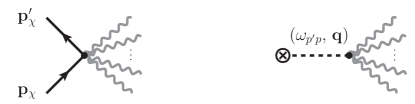
Figure 5: The effects of the incident DM particle on the target material can be regarded as an external field.

The coupling term in the action between the DM particle and nuclei in solids can be directly written as

$$\mathcal{V}_{\chi N} = -\int\mathrm{\,d}^{4}x\,\mathrm{\,d}^{4}x^{\prime}\,\psi_{\chi}^{*}\left(x\right)\psi_{\chi}\left(x\right)\,V_{\chi N}\left(x-x^{\prime}\right)\,\sum_{\boldsymbol{\ell}}\delta^{3}\left(\mathbf{x}^{\prime}-\boldsymbol{\ell}-\mathbf{u}_{\boldsymbol{\ell}}\right),$$ (A.31)

where the interaction is instantaneous such that $V_{\chi N}\left(x-x^{\prime}\right)=V_{\chi N}\left(\mathbf{x}-\mathbf{x}^{\prime}\right)\,\delta\left(t-t^{\prime}\right)$. Since one is only interested in the target material that hosts the phonons and electrons, it is convenient to integrate out the DM component and regard it as an external field. To be specific, one draws DM external field from the amplitude of the scattering process $\chi\left(\mathbf{p}_{\chi}\right)+$target$\rightarrow$$\chi\left(\mathbf{p}^{\prime}_{\chi}\right)+$target (excited) (see Fig. 5 for illustration) and obtains the effective Lagrangian

$$L_{\chi\mathrm{phonon}} = -\frac{V_{\chi N}\left(\mathbf{q}\right)e^{i\omega_{p^{\prime}p}t}}{V}\left[\int\mathrm{d}^{3}x^{\prime}\,e^{-i\mathbf{q}\cdot\mathbf{x}^{\prime}}\,\sum_{\boldsymbol{\ell}}\delta^{3}\left(\mathbf{x}^{\prime}-\boldsymbol{\ell}-\mathbf{u}_{\boldsymbol{\ell}}\left(t\right)\right)\right]$$

$$= -\frac{V_{\chi N}\left(\mathbf{q}\right)e^{i\omega_{p^{\prime}p}t}}{V}\sum_{\boldsymbol{\ell}}e^{-i\mathbf{q}\cdot\left(\boldsymbol{\ell}+\mathbf{u}_{\boldsymbol{\ell}}\left(t\right)\right)}$$

$$= -\frac{V_{\chi N}\left(\mathbf{q}\right)e^{i\omega_{p^{\prime}p}t}}{V}\sum_{s=0}^{+\infty}\frac{1}{s!}\sum_{\left\{\mathbf{p}_{j},\,\beta_{j}\,;s\right\}}\sum_{\boldsymbol{\ell}}e^{i\left(\sum_{j}\mathbf{p}_{j}-\mathbf{q}\right)\cdot\boldsymbol{\ell}}\left(\frac{-i\mathbf{q}\cdot\mathbf{\boldsymbol{\epsilon}}_{\mathbf{p}_{1},\beta_{1}}}{\sqrt{N\,m_{N}}}\right)\cdots\left(\frac{-i\mathbf{q}\cdot\mathbf{\boldsymbol{\epsilon}}_{\mathbf{p}_{s},\beta_{s}}}{\sqrt{N\,m_{N}}}\right)Q_{\mathbf{p}_{1},\beta_{1}}\cdots Q_{\mathbf{p}_{s},\beta_{s}}$$

$$= -\frac{V_{\chi N}\left(\mathbf{q}\right)e^{i\omega_{p^{\prime}p}t}}{V}\sum_{s=0}^{+\infty}\frac{1}{s!}\sum_{\left\{\mathbf{p}_{j},\,\beta_{j}\,;s\right\}}N\,\sum_{\mathbf{G}}\delta_{\sum_{j}\mathbf{p}_{j}-\mathbf{q},\,\mathbf{G}}\left(\frac{-i\mathbf{q}\cdot\mathbf{\boldsymbol{\epsilon}}_{\mathbf{p}_{1},\beta_{1}}}{\sqrt{N\,m_{N}}}\right)\cdots\left(\frac{-i\mathbf{q}\cdot\mathbf{\boldsymbol{\epsilon}}_{\mathbf{p}_{s},\beta_{s}}}{\sqrt{N\,m_{N}}}\right)Q_{\mathbf{p}_{1},\beta_{1}}\cdots Q_{\mathbf{p}_{s},\beta_{s}},$$

where $\mathbf{q}=\mathbf{p}^{\prime}_{\chi}-\mathbf{p}_{\chi}$, and $\omega_{p^{\prime}p}=\left|\mathbf{p}^{\prime}_{\chi}\right|^{2}/2\,m_{\chi}-\left|\mathbf{p}{}_{\chi}\right|^{2}/2\,m_{\chi}$, and $V_{\chi N}\left(\mathbf{q}\right)$ is the Fourier transform of the DM-nucleus contact interaction $V_{\chi N}\left(\mathbf{x}\right)$. It should be noted that in above discussion we adopt the discrete momentum convention.

Based on above discussion, one can derive the LSZ reduction formula for the multi-phonon scattering process. For example, the S-matrix for an $n$-phonon scattering process subject to a DM external field can be expressed as

$$-i\int\mathrm{d}t\,\frac{V_{\chi N}\left(\mathbf{q}\right)e^{i\omega_{p^{\prime}p}t}}{V}\sum_{s=0}^{+\infty}\frac{1}{s!}\,\sum_{\left\{\mathbf{p}_{j},\,\beta_{j}\,;s\right\}}N\,\sum_{\mathbf{G}}\delta_{\sum_{j}\mathbf{p}_{j}-\mathbf{q},\,\mathbf{G}}\,\prod_{i=1}^{n}\int\mathrm{d}t_{i}\,e^{i\omega_{\mathbf{k}_{i},\alpha_{i}}t_{i}}\frac{i}{\sqrt{2\,\omega_{\mathbf{k}_{i},\alpha_{i}}}}\overrightarrow{\left(\frac{\partial^{2}}{\partial t_{i}^{2}}+\omega_{\mathbf{k}_{i},\alpha_{i}}^{2}\right)}\,$$

$$\times\left.\overrightarrow{\frac{\delta}{\delta iJ_{\mathbf{k}_{1},\alpha_{1}}}}\cdots\overrightarrow{\frac{\delta}{\delta iJ_{\mathbf{k}_{n},\alpha_{n}}}}\left[e^{\sum_{\mathbf{k},\alpha}iJ_{\mathbf{k},\alpha}\frac{iD_{\mathbf{k},\alpha}}{2}iJ_{-\mathbf{k},\alpha}}\right]\overleftarrow{\frac{\delta}{\delta iJ_{\mathbf{p}_{1},\beta_{1}}}}\cdots\overleftarrow{\frac{\delta}{\delta iJ_{\mathbf{p}_{s},\beta_{s}}}}\right|_{J=0}\left(\frac{-i\mathbf{q}\cdot\mathbf{\boldsymbol{\epsilon}}_{\mathbf{p}_{1},\beta_{1}}}{\sqrt{N\,m_{N}}}\right)\cdots\left(\frac{-i\mathbf{q}\cdot\mathbf{\boldsymbol{\epsilon}}_{\mathbf{p}_{s},\beta_{s}}}{\sqrt{N\,m_{N}}}\right),$$

(A.33)

where $\left\{\mathbf{k}_{i},\alpha_{i}\right\}\,\left(i=1,\,2,\cdots,\,n\right)$ label the $n$-phonon final states.

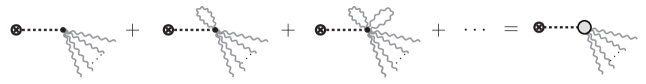
Figure 6: The diagram for the $n$-phonon scattering process containing full contributions of phonon loops, which generates the Debye-Waller factor denoted as the gray blob on the right-hand-side of the equation. See text for details.

Now one is able to investigate the amplitude for the full $n$-phonon scattering process shown in Fig. 6, which contains not only the tree level piece, but also higher orders of the phonon loop. Note that a self-closed propagator for mode $\left(\mathbf{k},\alpha\right)$ reads as

$$iD_{\mathbf{k},\alpha}\left(t^{+}-t\right) = \int_{-\infty}^{+\infty}\frac{i}{\omega^{2}-\omega_{\mathbf{k},\alpha}^{2}+i0^{+}}\frac{e^{-i0^{+}\omega}\mathrm{d}\omega}{2\pi}$$ (A.34)

$$= \frac{1}{2\,\omega_{\mathbf{k},\alpha}},$$

as well as a companion factor $\left(\frac{-i\mathbf{q}\cdot\mathbf{\boldsymbol{\epsilon}}_{\mathbf{k},\alpha}}{\sqrt{N\,m_{N}}}\right)\left(\frac{-i\mathbf{q}\cdot\mathbf{\boldsymbol{\epsilon}}_{\mathbf{k},\alpha}}{\sqrt{N\,m_{N}}}\right)$. Thus every loop in diagram corresponds to a factor $-\sum_{\mathbf{k},\alpha}\frac{\left|\mathbf{q}\cdot\mathbf{\boldsymbol{\epsilon}}_{\mathbf{k},\alpha}\right|^{2}}{2N\,m_{N}\omega_{\mathbf{k},\alpha}}$. On the other hand, a specific external leg $\left(\mathbf{k}_{i},\alpha_{i}\right)$ corresponds to

$$\int\mathrm{d}t_{i}\,e^{i\omega_{\mathbf{k}_{i},\alpha_{i}}t_{i}}\frac{i}{\sqrt{2\,\omega_{\mathbf{k}_{i},\alpha_{i}}}}\overrightarrow{\left(\frac{\partial^{2}}{\partial t_{i}^{2}}+\omega_{\mathbf{k}_{i},\alpha_{i}}^{2}\right)}\,iD_{\mathbf{k}_{i},\alpha_{i}}\left(t_{i}-t\right) = \frac{e^{i\omega_{\mathbf{k}_{i},\alpha_{i}}t}}{\sqrt{2\,\omega_{\mathbf{k}_{i},\alpha_{i}}}}.$$ (A.35)

Besides, the effect of the symmetry factor should also be taken into account. For example, one considers the $n$-phonon process containing $m$ self-interacting loops in Fig. 6. Determining the number of the contractions in Eq. (A.33) is equivalent to enumerating all possible ways the internal phonon lines interconnect among themselves, which is illustrated in Fig. 7. It is not difficult to verify that the overall constant that encodes the symmetry effect is equal to $\frac{\left(2m\right)!}{m!\,2^{m}}C_{n+2m}^{2m}\frac{n!}{\left(n+2m\right)!}=\frac{1}{m!\,2^{m}}$, where $C_{n+2m}^{2m}$counts which $2m$ lines self-connect among all $n+2m$ lines from the left in Fig. 7, $\frac{\left(2m\right)!}{m!\,2^{m}}$ is the number of the ways these specific $2m$ lines connect with each other, $n!$ describes the interchange of the external legs at the right hand in Fig. 7, and $\frac{1}{\left(n+2m\right)!}$ corresponds to the factor $\frac{1}{s!}$ in Eq. (A.33).

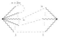
Figure 7: Illustration of possible ways in which $n$ phonon external lines connect to the $n$ internal ones while the left $2m$ internal members self-connect with each other to form $m$ loops. See text for details.

Putting all these pieces together, the sum of all diagrams on the left-hand-side in Fig. 6 can be expressed as

$$\left(-i\right)\frac{V_{\chi N}\left(\mathbf{q}\right)}{V}N\,\sum_{\mathbf{G}}\delta_{\sum_{i}\mathbf{k}_{i}+\mathbf{q},\,\mathbf{G}}\,\prod_{i=1}^{n}\left(\frac{-i\mathbf{q}\cdot\mathbf{\boldsymbol{\epsilon}}_{\mathbf{k}_{i},\alpha_{i}}}{\sqrt{2\,N\,m_{N}\omega_{\mathbf{k}_{i},\alpha_{i}}}}\right)\sum_{m=0}^{+\infty}\frac{1}{m!}\,\left(-\sum_{\mathbf{k},\alpha}\frac{\left|\mathbf{q}\cdot\mathbf{\boldsymbol{\epsilon}}_{\mathbf{k},\alpha}\right|^{2}}{4N\,m_{N}\omega_{\mathbf{k},\alpha}}\right)^{m}\int e^{i\left(\sum_{i}\omega_{\mathbf{k}_{i},\alpha_{i}}+\omega_{p^{\prime}p}\right)t}\mathrm{d}t$$ (A.36)

$$= \left(-i\right)\frac{V_{\chi N}\left(\mathbf{q}\right)}{V}N\,\sum_{\mathbf{G}}\delta_{\sum_{i}\mathbf{k}_{i}+\mathbf{q},\,\mathbf{G}}\,\prod_{i=1}^{n}\left(\frac{-i\mathbf{q}\cdot\mathbf{\boldsymbol{\epsilon}}_{\mathbf{k}_{i},\alpha_{i}}}{\sqrt{2\,N\,m_{N}\omega_{\mathbf{k}_{i},\alpha_{i}}}}\right)e^{-\sum_{\mathbf{k},\alpha}\frac{\left|\mathbf{q}\cdot\mathbf{\boldsymbol{\epsilon}}_{\mathbf{k},\alpha}\right|^{2}}{4Nm_{N}\omega_{\mathbf{k},\alpha}}}\,2\pi\delta\left(\sum_{i}\omega_{\mathbf{k}_{i},\alpha_{i}}+\omega_{p^{\prime}p}\right),$$

where $e^{-\sum_{\mathbf{k},\alpha}\frac{\left|\mathbf{q}\cdot\mathbf{\boldsymbol{\epsilon}}_{\mathbf{k},\alpha}\right|^{2}}{4Nm_{N}\omega_{\mathbf{k},\alpha}}}$ is no other than the Debye-Waller factor at the zero-temperature, which is represented with the gray blob on the right-hand-side of Fig. 6. In the derivation we interchange $\mathbf{\boldsymbol{\epsilon}}_{\mathbf{k},\alpha}$ and $\mathbf{\boldsymbol{\epsilon}}_{-\mathbf{k},\alpha}$ whenever necessary. From above discussion we can see one benefit of the path integral approach: one no longer has to resort to the cumbersome operator commutator algebra to obtain the Debye-Waller factor. Propagators do the job.

A.4 Electron-phonon interaction

The interaction between the ions and electrons can be directly written as

$$V_{\mathrm{ion}-e}\left(\mathbf{x}\right) = \sum_{\boldsymbol{\ell}}U_{e}\left(\mathbf{x}-\boldsymbol{\ell}-\mathbf{u}_{\boldsymbol{\ell}}\right)$$ (A.37)

$$= \sum_{\boldsymbol{\ell}}U_{e}\left(\mathbf{x}-\boldsymbol{\ell}\right)+\sum_{\boldsymbol{\ell}}\left(-\mathbf{u}_{\boldsymbol{\ell}}\right)\cdot\nabla U_{e}\left(\mathbf{x}-\boldsymbol{\ell}\right),$$

where $U_{e}\left(\mathbf{x}-\boldsymbol{\ell}\right)=-Z_{\mathrm{ion}}\alpha_{e}/\left|\mathbf{x}-\boldsymbol{\ell}\right|$ is Coulomb potential between the ion located at $\boldsymbol{\ell}$ and an electron at position $\mathbf{x}$. Thus, the electron-phonon interaction Lagrangian term is written as

$$\mathcal{L}_{\mathrm{phonon}-e} = \psi_{e}^{*}\left(x\right)\psi_{e}\left(x\right)\sum_{\boldsymbol{\ell}}\mathbf{u}_{\boldsymbol{\ell}}\cdot\nabla U_{e}\left(\mathbf{x}-\boldsymbol{\ell}\right)$$ (A.38)

$$= \psi_{e}^{*}\left(x\right)\psi_{e}\left(x\right)\sum_{\mathbf{k},\alpha}\mathbf{\boldsymbol{\epsilon}}_{\mathbf{k},\alpha}\cdot\nabla\left[\sum_{\boldsymbol{\ell}}U_{e}\left(\mathbf{x}-\boldsymbol{\ell}\right)e^{i\mathbf{k}\cdot\boldsymbol{\ell}}\right]\frac{Q_{\mathbf{k},\alpha}}{\sqrt{N\,m_{N}}}$$

$$= -\left(\frac{NZ_{\mathrm{ion}}}{V}\right)\psi_{e}^{*}\left(x\right)\psi_{e}\left(x\right)\,\sum_{\mathbf{k},\alpha}\sum_{\mathbf{G}}i\,\mathbf{\boldsymbol{\epsilon}}_{\mathbf{k},\alpha}\cdot\left(\mathbf{k}+\mathbf{G}\right)\,v\left(\mathbf{k}+\mathbf{G}\right)\,e^{i\mathbf{\left(\mathbf{k}+\mathbf{G}\right)}\cdot\mathbf{x}}\,\frac{Q_{\mathbf{k},\alpha}}{\sqrt{N\,m_{N}}},$$

with $v\left(\mathbf{k}+\mathbf{G}\right)=4\pi\alpha_{e}/\left|\mathbf{k}+\mathbf{G}\right|^{2}$.

A.5 Feynman rules

Based upon above preparation, the Feynman rules describing the processes involving multi-phonon and electron-phonon interactions in momentum space can be summarized as follows.

• In discussion the vertex of the DM particle is replaced with an external field as shown in Fig. 5. Such an external source corresponds $\left(-i\right)V_{\chi N}\left(\mathbf{q}\right)/V$.

• A gray blob corresponds to the factor $e^{-W\left(\mathbf{q}\right)}=e^{-\sum_{\mathbf{k},\alpha}\frac{\left|\mathbf{q}\cdot\mathbf{\boldsymbol{\epsilon}}_{\mathbf{k},\alpha}\right|^{2}}{4Nm_{N}\omega_{\mathbf{k},\alpha}}}$.

• Each blob also contributes the energy-momentum conservation condition presented as discrete delta functions $N\,\sum_{\mathbf{G}}\delta_{\sum_{i}\mathbf{p}_{i},\,\mathbf{G}}\,2\pi\delta\left(\sum\varepsilon_{i}\right)$, with $\left\{\mathbf{p}_{i}\right\}$ ($\left\{\varepsilon_{i}\right\}$) being the momenta (energies) flowing out of the blob.

• A phonon external leg representing the final state $\left(\mathbf{k}_{i},\alpha_{i}\right)$ from the blob corresponds to $\frac{-i\mathbf{q}\cdot\mathbf{\boldsymbol{\epsilon}}_{\mathbf{k}_{i},\alpha_{i}}}{\sqrt{2Nm_{N}\omega_{\mathbf{k}_{i},\alpha_{i}}}}$; a phonon internal line with mode $\left(\mathbf{k},\alpha\right)$ connecting the blob comes with a factor $\frac{-i\mathbf{q}\cdot\mathbf{\boldsymbol{\epsilon}}_{\mathbf{k},\alpha}}{\sqrt{Nm_{N}}}$.

• Each phonon internal line contributes a factor $1/2\pi$.

• Vertex that contains both the incoming and outgoing states ($\ket{j}$ and $\ket{i}$) of the electrons in solids contributes a factor $\left(2\pi\right)\braket{i}{e^{i\mathbf{p}\cdot\hat{\mathbf{x}}}}{j}$ and the energy conservation condition $\delta\left(\sum_{i}\varepsilon_{i}\right)$, where $\mathbf{p}$ is the net momentum sinking into the vertex.

• A phonon-electron vertex is read as

  $$\left(-NZ_{\mathrm{ion}}\right)\sum_{\mathbf{G}}\frac{i\,\mathbf{\boldsymbol{\epsilon}}_{\mathbf{k},\alpha}\cdot\left(\mathbf{k}+\mathbf{G}\right)}{\sqrt{Nm_{N}}}\frac{v\left(\mathbf{k}+\mathbf{G}\right)}{V}\braket{i}{e^{i\left(\mathbf{k}+\mathbf{G}\right)\cdot\hat{\mathbf{x}}}}{j}.$$

• A phonon internal line with one end connecting a phonon blob and the other connecting an electron vertex corresponds to the sum over propagators of all modes $\left\{\mathbf{k},\alpha\right\}$, i.e.,

  $$\sum_{\mathbf{k},\alpha}\left(\frac{-i\mathbf{q}\cdot\mathbf{\boldsymbol{\epsilon}}_{\mathbf{k},\alpha}}{\sqrt{Nm_{N}}}\right)\left(\frac{i}{\omega^{2}-\omega_{\mathbf{k},\alpha}^{2}+i0^{+}}\right)\left[\sum_{\mathbf{G}}\frac{i\,\mathbf{\boldsymbol{\epsilon}}_{\mathbf{k},\alpha}\cdot\left(\mathbf{k}+\mathbf{G}\right)}{\sqrt{Nm_{N}}}\frac{\left(-NZ_{\mathrm{ion}}\right)}{V}v\left(\mathbf{k}+\mathbf{G}\right)\braket{i}{e^{i\left(\mathbf{k}+\mathbf{G}\right)\cdot\hat{\mathbf{x}}}}{j}\right].$$

A.6 Random phase approximation

A short review of the random phase approximation (RPA) has been provided in Ref. [51], so here we only summarize some results relevant for our present discussion. Within the framework of the RPA, the Lindhard dielectric function for homogeneous electron gas (HEG) is expressed as

$$\epsilon\left(\mathbf{q},\omega\right) = 1-\frac{v\left(\mathbf{q}\right)}{V}\sum_{i,j}\frac{\left|\braket{i}{e^{i\mathbf{q}\cdot\hat{\mathbf{x}}}}{j}\right|^{2}}{\varepsilon_{i}-\varepsilon_{j}-\omega-i0^{+}}\left(n_{i}-n_{j}\right),$$ (A.39)

where $n_{i}$ ($n_{j}$) denotes the occupation number of the state $\ket{i}$ ($\ket{j}$), with $\varepsilon_{i}$ ($\varepsilon_{j}$) being corresponding eigenenergy. In crystalline structure the translational symmetry for space-time reduces to that for the periodic crystal lattice. The momentum transfer $\mathbf{q}$ in Eq. (A.39) is expressed uniquely as the sum of a reciprocal lattice vector $\mathbf{G}$, and corresponding reduced momentum $\mathbf{\mathbf{k}}$ confined in the 1BZ, i.e., $\mathbf{q}=\mathbf{k}+\mathbf{G}$. In this case, the microscopic dielectric matrix

$$\widetilde{\epsilon}_{\mathbf{G},\mathbf{G}^{\prime}}\left(\mathbf{\mathbf{k}},\omega\right) = \delta_{\mathbf{G},\mathbf{G}^{\prime}}-\frac{1}{V}\frac{4\pi\alpha_{e}}{\left|\mathbf{\mathbf{k}}+\mathbf{G}\right|\left|\mathbf{\mathbf{k}}+\mathbf{G}^{\prime}\right|}\sum_{i,j}\frac{\braket{i}{e^{i\left(\mathbf{\mathbf{\mathbf{\mathbf{k}}+\mathbf{G}}}^{\prime}\right)\cdot\hat{\mathbf{x}}}}{j}\braket{j}{e^{-i\left(\mathbf{\mathbf{k+\mathbf{G}}}\right)\cdot\hat{\mathbf{x}}}}{i}}{\varepsilon_{i}-\varepsilon_{j}-\omega-i0^{+}}\left(n_{i}-n_{j}\right)$$

is used to describe the screening effect in solids. For more details, see Ref. [51].

A.7 Electron-phonon interaction renormalization at the RPA level

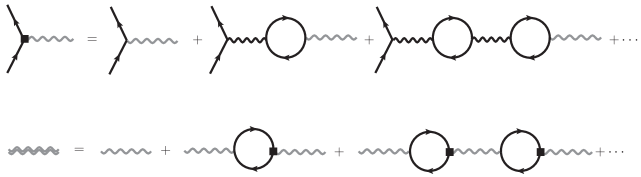
Figure 8: Top: The renormalized electron-phonon vertex (black square box) presented at the RPA level, where the one-particle-irreducible blob is represented by an electron-hole pair loop. Note that the gray lines represent the phonon propagators, while the black wiggly lines represent the Coulomb interaction. Bottom: The dressed phonon line (double wiggly line) presented at the RPA level. See text for details.

Here we discuss how to renormalize both the bare phonon propagator and effective electron-phonon interaction at the RPA level. In RPA, the polarization bubble is approximated as a simple electron-hole pair bubble, and hence the dressed electron-phonon vertex shown in the top row of Fig. 8 can be expressed (when the reciprocal lattice vectors are suppressed) as the sum

$$\frac{i\mathbf{\boldsymbol{\epsilon}}_{\mathbf{k},\alpha}\cdot\mathbf{k}}{\sqrt{N\,m_{N}}}\,\braket{i}{e^{i\mathbf{k}\cdot\hat{\mathbf{x}}}}{j}\,\left\{1+iv\left(\mathbf{k}\right)\left(-i\right)\Pi\left(\mathbf{k},\,\omega\right)+\left[iv\left(\mathbf{k}\right)\left(-i\right)\Pi\left(\mathbf{k},\,\omega\right)\right]^{2}+\cdots\right\}\left(-NZ_{\mathrm{ion}}\right)\frac{v\left(\mathbf{k}\right)}{V}$$ (A.41)

$$= \frac{i\mathbf{\boldsymbol{\epsilon}}_{\mathbf{k},\alpha}\cdot\mathbf{k}}{\sqrt{N\,m_{N}}}\,\braket{i}{e^{i\mathbf{k}\cdot\hat{\mathbf{x}}}}{j}\,\left[\frac{1}{1-v\left(\mathbf{k}\right)\Pi\left(\mathbf{k},\,\omega\right)}\right]\left(-NZ_{\mathrm{ion}}\right)\frac{v\left(\mathbf{k}\right)}{V}$$

$$= \frac{i\mathbf{\boldsymbol{\epsilon}}_{\mathbf{k},\alpha}\cdot\mathbf{k}}{\sqrt{N\,m_{N}}}\,\braket{i}{e^{i\mathbf{k}\cdot\hat{\mathbf{x}}}}{j}\,\frac{\left(-NZ_{\mathrm{ion}}\right)}{V}\,\frac{v\left(\mathbf{k}\right)}{\epsilon\left(\mathbf{k},\,\omega\right)},$$

where $\left(-i\right)\Pi$ corresponds to the electron-hole loop. It is evident that the effect of the normalization is suppressing the bare vertex with the dielectric function $\epsilon\left(\mathbf{k},\,\omega\right)$. The electron-phonon interaction also bring about a correction to the position of the phonon poles (in the RPA), as shown in the bottom row of Fig. 8. Since the typical band gaps are much larger than the phonon eigenenergies, these small corrections are irrelevant for our purpose in this study. One can use the $\mathtt{DarkELF}$ package to take into account the screening effect in various materials [70].

A.8 Asymptotic behavior of the multi-phonon distribution

Here we investigate the asymptotic behavior of the combined distribution of $n$ independent Poisson distributions encountered in Sec. 2, which justifies the validity of the impulse approximation in the large $q$ regime. To make the discussion concise, the following parameters are introduced: $\epsilon_{i}\sim\frac{\omega_{i}}{\overline{\omega}}$, $\mu_{i}\sim\left(\frac{1}{3N}\right)\frac{1}{\epsilon_{i}}$, $\lambda\sim\frac{q^{2}}{2m_{N}\overline{\omega}}$, $x\sim\frac{\omega}{\overline{\omega}\lambda}$, $\mu\sim\sum_{i=1}^{3N}\mu_{i}\epsilon_{i}=1$, $\sigma^{2}\sim\sum_{i=1}^{3N}\mu_{i}\epsilon_{i}^{2}=1$, and then consider the distribution

$$P\left(n_{1},\,n_{2},\cdots,\,n_{3N}\right) = p\left(n_{1},\lambda\mu_{1}\right)p\left(n_{2},\lambda\mu_{2}\right)\cdots p\left(n_{3N},\lambda\mu_{3N}\right)$$ (A.42)

$$= \frac{\left(\lambda\mu_{1}\right)^{n_{1}}}{n_{1}!}e^{-\lambda\mu_{1}}\cdots\frac{\left(\lambda\mu_{3N}\right)^{n_{3N}}}{n_{3N}!}e^{-\lambda\mu_{3N}},$$

where $p\left(n_{i},\lambda\mu_{i}\right)$ is the Poisson distribution of variable $n_{i}$ with mean $\lambda\mu_{i}$. We first try to obtain the distribution of a random variable in the form of $z=\sum_{i=1}^{3N}\left(\epsilon_{i}/\lambda\right)n_{i}$, and $\lambda$ being a parameter that characterizes the scale of the problem. To achieve this goal, we calculate the relevant characteristic function

$$\varphi_{Z}\left(t\right) = \sum_{\left\{n_{i}\right\}}P\left(n_{1},\,n_{2},\cdots,\,n_{3N}\right)e^{i\,zt}$$ (A.43)

$$= \prod_{i=1}^{3N}\left(\sum_{n_{i}=0}^{+\infty}\frac{\left(\lambda\mu_{i}\right)^{n_{i}}}{n_{i}!}e^{-\lambda\mu_{i}}e^{i\left(\epsilon_{i}/\lambda\right)n_{i}t}\right)$$

$$= \exp\left[\sum_{i=1}^{3N}\lambda\mu_{i}\left(e^{i\left(\epsilon_{i}/\lambda\right)t}-1\right)\right],$$

with which the distribution of the variable $x$ is explicitly expressed and expanded in $\lambda\,\left(\lambda\gg 1\right)$ as follows,

$$\Phi\left(x\right) = \frac{1}{2\pi}\int_{-\infty}^{+\infty}\varphi_{Z}\left(t\right)e^{-i\,xt}\mathrm{d}t$$

$$= \int_{-\infty}^{+\infty}\frac{\mathrm{d}t}{2\pi}\exp\left[\sum_{i=1}^{3N}\lambda\mu_{i}\left(e^{i\left(\epsilon_{i}/\lambda\right)t}-1\right)-i\,xt\right]$$

$$= \int_{-\infty}^{+\infty}\frac{\mathrm{d}t}{2\pi}\exp\left[-i\,(x-1)t-\left(\frac{1}{\lambda}\sum_{i=1}^{3N}\mu_{i}\epsilon_{i}^{2}\right)\frac{t^{2}}{2}\right]\cdot\left[1-i\left(\frac{1}{\lambda^{2}}\sum_{i=1}^{3N}\mu_{i}\epsilon_{i}^{3}\right)\frac{t^{3}}{3!}+o\left(\frac{1}{\lambda^{2}}\right)\right]$$

$$= \int_{-\infty}^{+\infty}\frac{\mathrm{d}z}{\sqrt{2\pi}}\exp\left\{-\frac{1}{2}\left[z+i\sqrt{\lambda}\,\left(x-1\right)\right]^{2}\right\}\cdot\left[1-\frac{i}{\sqrt{\lambda}}\left(\sum_{i=1}^{3N}\mu_{i}\epsilon_{i}^{3}\right)\frac{z^{3}}{3!}+o\left(\frac{1}{\sqrt{\lambda}}\right)\right]$$

$$\times\frac{1}{\sqrt{2\pi}/\sqrt{\lambda}}\exp\left[\frac{-\left(x-1\right)^{2}}{2/\lambda}\right]$$

$$= \frac{1}{\sqrt{2\pi}/\sqrt{\lambda}}\exp\left[\frac{-\left(x-1\right)^{2}}{2/\lambda}\right]\times\left\{1+\frac{1}{6}\left(\sum_{i=1}^{3N}\mu_{i}\epsilon_{i}^{3}\right)\left(x-1\right)\left[\lambda\left(x-1\right)^{2}-3\right]+o\left(\frac{1}{\sqrt{\lambda}}\right)\right\},$$

where $\sum_{i=1}^{3N}\mu_{i}\epsilon_{i}^{3}=\sum_{i=1}^{3N}\left(\frac{1}{3N}\right)\left(\omega_{i}^{2}/\overline{\omega}^{2}\right)$ in the last line. The integral in the last step can be evaluated by integrating over its saddle point $z_{0}=-i\sqrt{\lambda}\left(x-1\right)$ along the path $\left(z_{0}-\infty,\,z_{0}+\infty\right)$, on which $z^{3}$ term is suppressed by $1/\sqrt{\lambda}$, as long as $\left|x-1\right|$ is not too much larger than the width $1/\sqrt{\lambda}$.

A.9 Iterative calculation of multi-phonon process

Here we discuss how to calculate the multi-phonon spectrum at $T=0\,\mathrm{K}$ following a recursive procedure. First, we explicitly derive the scattering factor introduced in Eq. (2.6) as the following,

$$S\left(q,\omega\right) = \sum_{\left\{n_{i}\right\}}\frac{e^{-\frac{E_{R}\left(q\right)}{3N\omega_{1}}}}{n_{1}!}\left(\frac{E_{R}\left(q\right)}{3N\omega_{1}}\right)^{n_{1}}\cdots\frac{e^{-\frac{E_{R}\left(q\right)}{3N\omega_{3N}}}}{n_{3N}!}\left(\frac{E_{R}\left(q\right)}{3N\omega_{3N}}\right)^{n_{3N}}\delta\left(\sum_{i=1}^{3N}n_{i}\omega_{i}-\omega\right)$$ (A.45)

$$= e^{-E_{R}\left(q\right)\sum_{i=1}^{3N}\frac{1}{3N}\frac{1}{\omega_{i}}}\left[\int_{-\infty}^{+\infty}\frac{e^{i\left(\sum_{i=1}^{3N}n_{i}\omega_{i}-\omega\right)t}}{2\pi}\mathrm{d}t\right]\times\left[\sum_{\left\{n_{i}\right\}}\frac{1}{n_{1}!}\left(\frac{E_{R}\left(q\right)}{3N\omega_{1}}\right)^{n_{1}}\cdots\frac{1}{n_{3N}!}\left(\frac{E_{R}\left(q\right)}{3N\omega_{3N}}\right)^{n_{3N}}\right]$$

$$= e^{-E_{R}\left(q\right)\sum_{i=1}^{3N}\frac{1}{3N}\frac{1}{\omega_{i}}}\int_{-\infty}^{+\infty}\mathrm{d}t\,\frac{e^{-i\omega t}}{2\pi}\times\left[\sum_{n=0}^{+\infty}\frac{E_{R}\left(q\right)^{n}}{n!}\left(\sum_{i=1}^{3N}\frac{1}{3N}\frac{e^{i\omega_{i}t}}{\omega_{i}}\right)^{n}\right]$$

$$= e^{-E_{R}\left(q\right)\sum_{i=1}^{3N}\frac{1}{3N}\frac{1}{\omega_{i}}}\int_{-\infty}^{+\infty}\mathrm{d}t\,\frac{e^{-i\omega t}}{2\pi}\times\left(\sum_{n=0}^{+\infty}\frac{E_{R}\left(q\right)^{n}}{n!}f\left(t\right)^{n}\right)$$

$$= e^{-E_{R}\left(q\right)\sum_{i=1}^{3N}\frac{1}{3N}\frac{1}{\omega_{i}}}\times\left(\sum_{n=0}^{+\infty}\frac{E_{R}\left(q\right)^{n}}{n!}\int_{-\infty}^{+\infty}\mathrm{d}t\,f\left(t\right)^{n}\frac{e^{-i\omega t}}{2\pi}\right)$$

$$= e^{-E_{R}\left(q\right)\sum_{i=1}^{3N}\frac{1}{3N}\frac{1}{\omega_{i}}}\times\left(\sum_{n=0}^{+\infty}\frac{E_{R}\left(q\right)^{n}}{n!}T_{n}\left(\omega\right)\right).$$

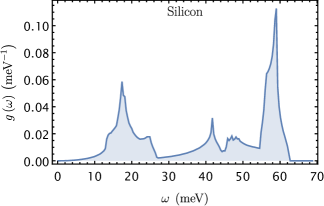
Figure 9: The normalized phonon density of states for bulk silicon. See text for details.

Then it is easy to verify the following recursive relation (see Ref. [62] for a general discussion on the case of a finite temperature)

$$\int_{-\infty}^{+\infty}T_{1}\left(\omega-\omega^{\prime}\right)T_{p-1}\left(\omega^{\prime}\right)\mathrm{d}\omega^{\prime} = \int_{-\infty}^{+\infty}\mathrm{d}\omega^{\prime}\int_{-\infty}^{+\infty}\mathrm{d}t\,f\left(t\right)\frac{e^{-i\left(\omega-\omega^{\prime}\right)t}}{2\pi}\int_{-\infty}^{+\infty}\mathrm{d}t^{\prime}\,f\left(t^{\prime}\right)^{p-1}\frac{e^{-i\omega^{\prime}t^{\prime}}}{2\pi}$$ (A.46)

$$= \frac{1}{2\pi}\int_{-\infty}^{+\infty}f\left(t\right)^{p}e^{-i\omega t}\mathrm{d}t$$

$$= T_{p}\left(\omega\right).$$

It is straightforward to see

$$T_{1}\left(\omega\right) = \int_{-\infty}^{+\infty}\mathrm{d}t\,f\left(t\right)\frac{e^{-i\omega t}}{2\pi}$$ (A.47)

$$= \int_{-\infty}^{+\infty}\mathrm{d}t\,\frac{1}{3N}\sum_{i=1}^{3N}\frac{1}{\omega_{i}}\frac{e^{i\left(\omega_{i}-\omega\right)t}}{2\pi}$$

$$= \frac{1}{3N}\sum_{i=1}^{3N}\frac{1}{\omega}\delta\left(\omega_{i}-\omega\right),$$

which means $T_{1}\left(\omega\right)=0,$ if $\omega<0$. This feature can be easily generalized to the case of an arbitrary $p$ such that $T_{p}\left(\omega\right)=0$, $\left(\omega<0\right)$. In practice, we utilize Eq. (A.46) to obtain $\left\{T_{n}\left(\omega\right)\right\}$ and to further calculate the spectrum of the multi-phonon process with Eq. (2.6). This recursive method requires only the phonon DoS for a solid target (e.g., for monatomic simple lattice) as follows,

$$g\left(\omega\right) = \frac{1}{3N}\sum_{i=1}^{3N}\delta\left(\omega_{i}-\omega\right),$$ (A.48)

which is normalized such that $\int_{0}^{+\infty}g\left(\omega\right)\mathrm{d}\omega=1$. For illustration, in Fig. 9 we present the normalized DoS for the bulk silicon, which is calculated using $\mathtt{PHONOPY}$ code [71], while the force constants are computed using $\mathtt{VASP}$ package [72] based on the density functional theory [73, 74] with Perdew, Burke, and Ernzerhof form [75] of the generalized gradient approximation on the exchange-correlation functional.

References

- [1] Y. Kahn and T. Lin, Searches for light dark matter using condensed matter systems, Rept. Prog. Phys. 85 (2022) 066901 [2108.03239].
- [2] R. Essig, J. Mardon and T. Volansky, Direct Detection of Sub-GeV Dark Matter, Phys. Rev. D85 (2012) 076007 [1108.5383].
- [3] P. W. Graham, D. E. Kaplan, S. Rajendran and M. T. Walters, Semiconductor Probes of Light Dark Matter, Phys. Dark Univ. 1 (2012) 32 [1203.2531].
- [4] R. Essig, M. Fernandez-Serra, J. Mardon, A. Soto, T. Volansky and T.-T. Yu, Direct Detection of sub-GeV Dark Matter with Semiconductor Targets, JHEP 05 (2016) 046 [1509.01598].
- [5] Y. Hochberg, T. Lin and K. M. Zurek, Absorption of light dark matter in semiconductors, Phys. Rev. D95 (2017) 023013 [1608.01994].
- [6] Y. Hochberg, Y. Kahn, M. Lisanti, K. M. Zurek, A. G. Grushin, R. Ilan et al., Detection of sub-MeV Dark Matter with Three-Dimensional Dirac Materials, Phys. Rev. D97 (2018) 015004 [1708.08929].
- [7] A. Coskuner, A. Mitridate, A. Olivares and K. M. Zurek, Directional Dark Matter Detection in Anisotropic Dirac Materials, Phys. Rev. D 103 (2021) 016006 [1909.09170].
- [8] R. M. Geilhufe, F. Kahlhoefer and M. W. Winkler, Dirac Materials for Sub-MeV Dark Matter Detection: New Targets and Improved Formalism, Phys. Rev. D 101 (2020) 055005 [1910.02091].
- [9] Y. Hochberg, Y. Zhao and K. M. Zurek, Superconducting Detectors for Superlight Dark Matter, Phys. Rev. Lett. 116 (2016) 011301 [1504.07237].
- [10] Y. Hochberg, T. Lin and K. M. Zurek, Detecting Ultralight Bosonic Dark Matter via Absorption in Superconductors, Phys. Rev. D94 (2016) 015019 [1604.06800].
- [11] S. Knapen, T. Lin and K. M. Zurek, Light Dark Matter in Superfluid Helium: Detection with Multi-excitation Production, Phys. Rev. D95 (2017) 056019 [1611.06228].
- [12] A. Caputo, A. Esposito and A. D. Polosa, Sub-MeV Dark Matter and the Goldstone Modes of Superfluid Helium, Phys. Rev. D 100 (2019) 116007 [1907.10635].
- [13] A. Caputo, A. Esposito, E. Geoffray, A. D. Polosa and S. Sun, Dark Matter, Dark Photon and Superfluid He-4 from Effective Field Theory, Phys. Lett. B 802 (2020) 135258 [1911.04511].
- [14] S. Griffin, S. Knapen, T. Lin and K. M. Zurek, Directional Detection of Light Dark Matter with Polar Materials, Phys. Rev. D98 (2018) 115034 [1807.10291].
- [15] S. Knapen, T. Lin, M. Pyle and K. M. Zurek, Detection of Light Dark Matter With Optical Phonons in Polar Materials, Phys. Lett. B785 (2018) 386 [1712.06598].
- [16] B. Campbell-Deem, P. Cox, S. Knapen, T. Lin and T. Melia, Multiphonon excitations from dark matter scattering in crystals, Phys. Rev. D 101 (2020) 036006 [1911.03482].
- [17] C. Kouvaris and J. Pradler, Probing sub-GeV Dark Matter with conventional detectors, Phys. Rev. Lett. 118 (2017) 031803 [1607.01789].
- [18] N. F. Bell, J. B. Dent, J. L. Newstead, S. Sabharwal and T. J. Weiler, Migdal effect and photon bremsstrahlung in effective field theories of dark matter direct detection and coherent elastic neutrino-nucleus scattering, Phys. Rev. D 101 (2020) 015012 [1905.00046].
- [19] R. Essig, A. Manalaysay, J. Mardon, P. Sorensen and T. Volansky, First Direct Detection Limits on sub-GeV Dark Matter from XENON10, Phys. Rev. Lett. 109 (2012) 021301 [1206.2644].
- [20] S. K. Lee, M. Lisanti, S. Mishra-Sharma and B. R. Safdi, Modulation Effects in Dark Matter-Electron Scattering Experiments, Phys. Rev. D92 (2015) 083517 [1508.07361].
- [21] Y. Hochberg, M. Pyle, Y. Zhao and K. M. Zurek, Detecting Superlight Dark Matter with Fermi-Degenerate Materials, JHEP 08 (2016) 057 [1512.04533].
- [22] I. M. Bloch, R. Essig, K. Tobioka, T. Volansky and T.-T. Yu, Searching for Dark Absorption with Direct Detection Experiments, JHEP 06 (2017) 087 [1608.02123].
- [23] S. Derenzo, R. Essig, A. Massari, A. Soto and T.-T. Yu, Direct Detection of sub-GeV Dark Matter with Scintillating Targets, Phys. Rev. D96 (2017) 016026 [1607.01009].
- [24] Y. Hochberg, Y. Kahn, M. Lisanti, C. G. Tully and K. M. Zurek, Directional detection of dark matter with two-dimensional targets, Phys. Lett. B772 (2017) 239 [1606.08849].
- [25] R. Essig, J. Mardon, O. Slone and T. Volansky, Detection of sub-GeV Dark Matter and Solar Neutrinos via Chemical-Bond Breaking, Phys. Rev. D95 (2017) 056011 [1608.02940].
- [26] F. Kadribasic, N. Mirabolfathi, K. Nordlund, A. E. Sand, E. Holmstrom and F. Djurabekova, Directional Sensitivity In Light-Mass Dark Matter Searches With Single-Electron Resolution Ionization Detectors, Phys. Rev. Lett. 120 (2018) 111301 [1703.05371].
- [27] R. Essig, T. Volansky and T.-T. Yu, New Constraints and Prospects for sub-GeV Dark Matter Scattering off Electrons in Xenon, Phys. Rev. D96 (2017) 043017 [1703.00910].
- [28] A. Arvanitaki, S. Dimopoulos and K. Van Tilburg, Resonant absorption of bosonic dark matter in molecules, Phys. Rev. X8 (2018) 041001 [1709.05354].
- [29] R. Budnik, O. Chesnovsky, O. Slone and T. Volansky, Direct Detection of Light Dark Matter and Solar Neutrinos via Color Center Production in Crystals, Phys. Lett. B782 (2018) 242 [1705.03016].
- [30] P. Sharma, Role of nuclear charge change and nuclear recoil on shaking processes and their possible implication on physical processes, Nuclear Physics A 968 (2017) 326 .
- [31] G. Cavoto, F. Luchetta and A. D. Polosa, Sub-GeV Dark Matter Detection with Electron Recoils in Carbon Nanotubes, Phys. Lett. B776 (2018) 338 [1706.02487].
- [32] Z.-L. Liang, L. Zhang, P. Zhang and F. Zheng, The wavefunction reconstruction effects in calculation of DM-induced electronic transition in semiconductor targets, JHEP 01 (2019) 149 [1810.13394].
- [33] M. Heikinheimo, K. Nordlund, K. Tuominen and N. Mirabolfathi, Velocity Dependent Dark Matter Interactions in Single-Electron Resolution Semiconductor Detectors with Directional Sensitivity, Phys. Rev. D99 (2019) 103018 [1903.08654].
- [34] T. Trickle, Z. Zhang, K. M. Zurek, K. Inzani and S. Griffin, Multi-Channel Direct Detection of Light Dark Matter: Theoretical Framework, JHEP 03 (2020) 036 [1910.08092].
- [35] T. Trickle, Z. Zhang and K. M. Zurek, Detecting Light Dark Matter with Magnons, Phys. Rev. Lett. 124 (2020) 201801 [1905.13744].
- [36] R. Catena, T. Emken, N. A. Spaldin and W. Tarantino, Atomic responses to general dark matter-electron interactions, Phys. Rev. Res. 2 (2020) 033195 [1912.08204].
- [37] E. Andersson, A. Bökmark, R. Catena, T. Emken, H. K. Moberg and E. Åstrand, Projected sensitivity to sub-GeV dark matter of next-generation semiconductor detectors, JCAP 05 (2020) 036 [2001.08910].
- [38] T. Trickle, Z. Zhang and K. M. Zurek, Effective field theory of dark matter direct detection with collective excitations, Phys. Rev. D 105 (2022) 015001 [2009.13534].
- [39] S. M. Griffin, Y. Hochberg, K. Inzani, N. Kurinsky, T. Lin and T. Chin, Silicon carbide detectors for sub-GeV dark matter, Phys. Rev. D 103 (2021) 075002 [2008.08560].
- [40] H.-Y. Chen, A. Mitridate, T. Trickle, Z. Zhang, M. Bernardi and K. M. Zurek, Dark Matter Direct Detection in Materials with Spin-Orbit Coupling, 2202.11716.
- [41] L. Hamaide and C. McCabe, Fuelling the search for light dark matter-electron scattering, 2110.02985.
- [42] W. Chao, M. Jin and Y.-Q. Peng, Direct detection of Sub-GeV Dark Matter via 3-body Inelastic Scattering Process, 2109.14944.
- [43] M. Ibe, W. Nakano, Y. Shoji and K. Suzuki, Migdal effect in dark matter direct detection experiments, Journal of High Energy Physics 2018 (2018) 194.
- [44] K. D. Nakamura, K. Miuchi, S. Kazama, Y. Shoji, M. Ibe and W. Nakano, Detection capability of the Migdal effect for argon and xenon nuclei with position-sensitive gaseous detectors, PTEP 2021 (2021) 013C01 [2009.05939].
- [45] P. Majewski et al., “Observation of the Migdal effect from nuclear scattering using a low pressure Optical-TPC.” https://indi.to/mK5zc, 2020. 10.1039/d2tc01222g.
- [46] C. A. J. O’Hare et al., Recoil imaging for dark matter, neutrinos, and physics beyond the Standard Model, in 2022 Snowmass Summer Study, 3, 2022, 2203.05914.
- [47] M. J. Dolan, F. Kahlhoefer and C. McCabe, Directly detecting sub-GeV dark matter with electrons from nuclear scattering, Phys. Rev. Lett. 121 (2018) 101801 [1711.09906].
- [48] R. Essig, J. Pradler, M. Sholapurkar and T.-T. Yu, Relation between the Migdal Effect and Dark Matter-Electron Scattering in Isolated Atoms and Semiconductors, Phys. Rev. Lett. 124 (2020) 021801 [1908.10881].
- [49] Z.-L. Liang, L. Zhang, F. Zheng and P. Zhang, Describing migdal effects in diamond crystal with atom-centered localized wannier functions, Phys. Rev. D 102 (2020) 043007.
- [50] S. Knapen, J. Kozaczuk and T. Lin, Migdal Effect in Semiconductors, Phys. Rev. Lett. 127 (2021) 081805 [2011.09496].
- [51] Z.-L. Liang, C. Mo, F. Zheng and P. Zhang, Describing the Migdal effect with a bremsstrahlung-like process and many-body effects, Phys. Rev. D 104 (2021) 056009 [2011.13352].
- [52] G. Grilli di Cortona, A. Messina and S. Piacentini, Migdal effect and photon Bremsstrahlung: improving the sensitivity to light dark matter of liquid argon experiments, JHEP 11 (2020) 034 [2006.02453].
- [53] C. P. Liu, C.-P. Wu, H.-C. Chi and J.-W. Chen, Model-independent determination of the Migdal effect via photoabsorption, Phys. Rev. D 102 (2020) 121303 [2007.10965].
- [54] V. V. Flambaum, L. Su, L. Wu and B. Zhu, Constraining sub-GeV dark matter from Migdal and Boosted effects, 2012.09751.
- [55] U. K. Dey, T. N. Maity and T. S. Ray, Prospects of Migdal Effect in the Explanation of XENON1T Electron Recoil Excess, Phys. Lett. B 811 (2020) 135900 [2006.12529].
- [56] W. Wang, K.-Y. Wu, L. Wu and B. Zhu, Direct Detection of Spin-Dependent Sub-GeV Dark Matter via Migdal Effect, 2112.06492.
- [57] XENON collaboration, Search for Light Dark Matter Interactions Enhanced by the Migdal Effect or Bremsstrahlung in XENON1T, Phys. Rev. Lett. 123 (2019) 241803 [1907.12771].
- [58] CDEX collaboration, Constraints on Spin-Independent Nucleus Scattering with sub-GeV Weakly Interacting Massive Particle Dark Matter from the CDEX-1B Experiment at the China Jinping Underground Laboratory, Phys. Rev. Lett. 123 (2019) 161301 [1905.00354].
- [59] EDELWEISS collaboration, First germanium-based constraints on sub-MeV Dark Matter with the EDELWEISS experiment, Phys. Rev. Lett. 125 (2020) 141301 [2003.01046].
- [60] COSINE-100 collaboration, Searching for low-mass dark matter via the Migdal effect in COSINE-100, Phys. Rev. D 105 (2022) 042006 [2110.05806].
- [61] SuperCDMS collaboration, A Search for Low-mass Dark Matter via Bremsstrahlung Radiation and the Migdal Effect in SuperCDMS, 2203.02594.
- [62] H. Schober, An introduction to the theory of nuclear neutron scatterin in condensed matter, Journal of Neutron Research (2014) 109.
- [63] Y. Kahn, G. Krnjaic and B. Mandava, Dark Matter Detection with Bound Nuclear Targets: The Poisson Phonon Tail, Phys. Rev. Lett. 127 (2021) 081804 [2011.09477].
- [64] K. V. Berghaus, R. Essig, Y. Hochberg, Y. Shoji and M. Sholapurkar, The Phonon Background from Gamma Rays in Sub-GeV Dark Matter Detectors, 2112.09702.
- [65] B. Campbell-Deem, S. Knapen, T. Lin and E. Villarama, Dark matter direct detection from the single phonon to the nuclear recoil regime, 2205.02250.
- [66] S. Knapen, J. Kozaczuk and T. Lin, Dark matter-electron scattering in dielectrics, Phys. Rev. D 104 (2021) 015031 [2101.08275].
- [67] D. Baxter et al., Recommended conventions for reporting results from direct dark matter searches, Eur. Phys. J. C 81 (2021) 907 [2105.00599].
- [68] K. V. Berghaus, R. Essig, A. Esposito, and M. Sholapurkar, The Migdal Effect in Semiconductors from Effective Field Theory, to appear .
- [69] H. Bruus and K. Flensberg, Many-body quantum theory in condensed matter physics, Oxford Graduate Texts. Oxford University Press, USA, 2004.
- [70] S. Knapen, J. Kozaczuk and T. Lin, python package for dark matter scattering in dielectric targets, Phys. Rev. D 105 (2022) 015014 [2104.12786].
- [71] A. Togo and I. Tanaka, First principles phonon calculations in materials science, Scripta Materialia 108 (2015) 1.
- [72] G. Kresse and J. Furthmüller, Efficient iterative schemes for ab initio total-energy calculations using a plane-wave basis set, Phys. Rev. B 54 (1996) 11169.
- [73] P. Hohenberg and W. Kohn, Inhomogeneous electron gas, Phys. Rev. 136 (1964) B864.
- [74] W. Kohn and L. J. Sham, Self-consistent equations including exchange and correlation effects, Phys. Rev. 140 (1965) A1133.
- [75] J. P. Perdew, K. Burke and M. Ernzerhof, Generalized gradient approximation made simple, Phys. Rev. Lett. 77 (1996) 3865.