Numerical Framework for New Langevin Noise Model: Applications to Plasmonic Hong-Ou-Mandel Effects

Abstract

We present a numerical framework of the new Langevin noise (LN) formalism [1, 2] leveraging computational electromagnetics numerical methods to analyze quantum electromagnetic systems involving both medium and radiation losses. We then perform fully quantum-theoretic numerical simulations to retrieve quantum plasmonic Hong-Ou-Mandel (HOM) effects, demonstrated in recent experimental works [3, 4, 5], due to plasmonic interferences of two indistinguishable bosonic particles occupied in surface plasmon polariton fields. The developed numerical framework would pave the path towards enabling quantitative evaluations of open and dissipative quantum optics problems with the medium inhomogeneity and geometric complexity, e.g., quantum plasmonic phenomena and metasurface-based devices, useful for advancing the current quantum optics technology.

Hong-Ou-Mandel (HOM) effects are widely used in quantum optics to quantify the indistinguishability of two photons [6]. When a pair of indistinguishable (input) photons simultaneously enters a 50:50 beam splitter and interfere, second-order correlations of the output photons drop to zero due to the creation of entanglement, which any classical lights can never mimic. More recently, several experimental works [3, 4, 5] have demonstrated that two indistinguishable bosonic particles occupied in surface plasmonic polariton (SPP) fields can also exhibit the HOM effects via plasmonic interferences, as depicted in Fig. 1. Most quantum optics technology is currently based on bulky photonic circuit components, .e.g, beam splitter or phase shifter. The preservation of the bosonic interferences indicates that the plasmonic technology would serve as a powerful alternative to integrating existing quantum optics systems into a small volume.

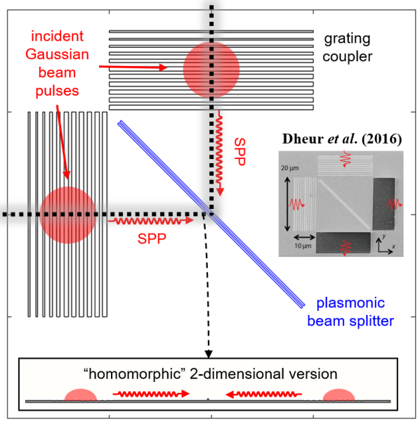
Figure 1: A plasmonic platform to observe quantum plasmonic Hong-Ou-Mandel effects (the inset figure on the right illustrating a scanning electron microscope image for the top view of the photon-to-surface-plasmon-polariton launcher was reproduced from [4]). The “homomorphic” 2-dimensional platform (the black-dashed line) can mimic the equivalent dynamics.

Metals (e.g., gold and silver) at optical wavelength and hybrid plasmonic metasurfaces are frequently used for plasmonic materials attributed to their preferable dispersion profiles. Their effective permittivity should satisfy the Kramers-Kronig relation to be causal; hence, the presence of ohmic losses is inevitable. In other words, one should account for both dispersion and ohmic loss effects when analyzing quantum plasmonic devices. However, such systems become non-Hermitian; the resulting eigenmodes do not support their orthonormal property and have real-valued eigenfrequencies. Consequently, the Hamiltonian operator cannot be diagonalized by ladder operators evolving without attenuation, and the bosonic commutators are not preserved in time. Therefore, one no longer relies on standard second quantization methods for harmonic oscillators [7, 8, 9, 10].

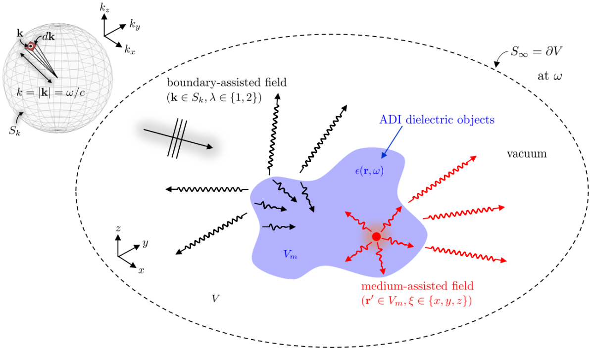
Figure 2: The new Langevin noise formalism [1, 2] employ two different fields for the quantization of open and dissipative electromagnetic systems : (i) boundary-assisted (BA) and (ii) medium-assisted (MA) fields to balance the radiation and medium losses. Monochromatic BA and MA fields form the infinite degeneracy in terms of ($\mathbf{k}\in S_{k}$, $\lambda\in\left\{1,2\right\}$) and ($\mathbf{r}\in V_{m},\xi\in\left\{x,y,z\right\}$), respectively.

To tackle such difficulties, the (previous) Langevin noise (LN) formalism [11, 12] has been proposed based on the macroscopic theory of quantum electrodynamics (QED) and fluctuation-dissipation theorem (FDT). Therein, electric field operators are now interpreted as the response to Langevin noise sources that are introduced to compensate the medium loss in an ensemble sense, called medium-assisted (MA) fields. However, practical quantum optics problems typically employ finite-sized nanostructures in the vacuum (or lossless background medium). Hence, one should take into account the radiation loss due to the open boundary. The radiation loss would serve as another source of making electromagnetic (EM) systems non-Hermitian in addition to the medium loss. The new Langevin noise (LN) approach [1, 2] is a great alternative for dealing with such open and dissipative quantum EM systems. Basically, the new LN model added a missing term, i.e., boundary-assisted (BA) fields, into the previous LN model to compensate the radiation loss, as illustrated in Fig. 2. As such, the new LN model fully agrees with the FDT in the presence of the two different losses.

According to the new LN model, for a lossy dielectric object described by $\epsilon(\mathbf{r},\omega)=\epsilon_{0}\bigl{(}1+\chi(\mathbf{r},\omega)\bigr{)}$, a complete electric field operator is expanded by both BAMA fields, (the positive frequency component) taking the form of $\hat{\mathbf{E}}^{(+)}(\mathbf{r},t)=\hat{\mathbf{E}}^{(+)}_{(BA)}(\mathbf{r},t)+\hat{\mathbf{E}}^{(+)}_{(MA)}(\mathbf{r},t)$ where

$$\hat{\mathbf{E}}^{(+)}_{(BA)}(\mathbf{r},t)=i\int_{0}^{\infty}d\omega\mathcal{B}(\omega)\int_{S_{k}}d\mathbf{k}\sum_{\lambda=1}^{2}\boldsymbol{\Phi}_{\mathbf{k},\lambda,\omega}(\mathbf{r})$$

$$\quad\quad\quad\quad\quad\quad\quad\quad\quad\quad\quad\times\hat{a}_{\mathbf{k},\lambda,\omega}e^{-i\omega t},$$ (1)

$$\hat{\mathbf{E}}^{(+)}_{(MA)}(\mathbf{r},t)=i\int_{0}^{\infty}d\omega\mathcal{C}(\omega)\int_{V_{m}}d\mathbf{r}^{\prime}\sum_{\xi\in\left\{x,y,z\right\}}\overline{\mathbf{G}}(\mathbf{r},\mathbf{r}^{\prime},\omega)\cdot\hat{\xi}$$

$$\quad\quad\quad\quad\quad\quad\quad\quad\quad\quad\quad\times\sqrt{\text{Im}\left(\epsilon(\mathbf{r}^{\prime},\omega)\right)}\hat{f}_{\mathbf{r}^{\prime},\xi,\omega}e^{-i\omega t}.$$ (2)

In the above, two frequency-dependent constants $\mathcal{B}(\omega)=(\sqrt{2\pi})^{-d}\sqrt{\hbar\omega/2}$ for $d$-dimensional space, and $\mathcal{C}(\omega)=(\omega^{2}/c^{2})\sqrt{\hbar/(\pi\epsilon_{0})}$. $S_{k}$ is the radiation sphere with the radius $k=\omega/c$ in $\mathbf{k}$-space. $\boldsymbol{\Phi}_{\mathbf{k},\lambda,\omega}(\mathbf{r})$ denotes a total field composed of (i) an incident plane wave with wavevector $\mathbf{k}\in S_{k}$ and polarization degenerate index $\lambda\in\left\{1,2\right\}$ in the vacuum, and (ii) scattered fields due to the lossy dielectric object, viz., $\boldsymbol{\Phi}_{\mathbf{k},\lambda,\omega}(\mathbf{r})=\boldsymbol{\Phi}^{\text{(inc)}}_{\mathbf{k},\lambda,\omega}(\mathbf{r})+\boldsymbol{\Phi}^{\text{(sca)}}_{\mathbf{k},\lambda,\omega}(\mathbf{r})$ from the following plane-wave-scattering problem [13]

$$\hat{S}\boldsymbol{\Phi}^{(\text{sca})}_{\mathbf{k},\lambda,\omega}(\mathbf{r})-\omega^{2}\epsilon(\mathbf{r},\omega)\boldsymbol{\Phi}^{(\text{sca})}_{\mathbf{k},\lambda,\omega}(\mathbf{r})=\omega^{2}\epsilon_{0}\chi(\mathbf{r},\omega)\boldsymbol{\Phi}^{(\text{inc})}_{\mathbf{k},\lambda,\omega}(\mathbf{r})$$ (3)

where $\hat{S}=\nabla\times\mu_{0}^{-1}\nabla\times$. $V_{m}$ is the volume of the lossy dielectric object, and $\overline{\mathbf{G}}(\mathbf{r},\mathbf{r}^{\prime},\omega)$ is a dyadic Green’s function from the following point-source-radiation problem

$$\hat{S}\overline{\mathbf{G}}(\mathbf{r},\mathbf{r}^{\prime},\omega)-\omega^{2}\epsilon(\mathbf{r},\omega)\overline{\mathbf{G}}(\mathbf{r},\mathbf{r}^{\prime},\omega)=\overline{\mathbf{I}}\delta(\mathbf{r}-\mathbf{r}^{\prime}).$$ (4)

Two different ladder operators, i.e., $\hat{a}_{\mathbf{k},\lambda,\omega}$ and $\hat{f}_{\mathbf{r}^{\prime},\xi,\omega}$, are associated with BA and MA fields, respectively, satisfy the standard bosonic commutator relations, and take multimode Fock states as eigenstates of their number operators. The Hamiltonian operator is then diagonalized by the two ladder operators [1, Eqn. (4.37)]

$$\hat{H} =\int_{0}^{\infty}d\omega\int_{S_{k}}d\mathbf{k}\sum_{\lambda=1}^{2}\hbar\omega\hat{a}^{{\dagger}}_{\mathbf{k},\lambda,\omega}\hat{a}_{\mathbf{k},\lambda,\omega}$$

$$+\int_{0}^{\infty}d\omega\int_{V_{m}}d\mathbf{r}^{\prime}\sum_{\xi\in\left\{x,y,z\right\}}\hbar\omega\hat{f}^{{\dagger}}_{\mathbf{r}^{\prime},\xi,\omega}\hat{f}_{\mathbf{r}^{\prime},\xi,\omega}.$$ (5)

Figure 3: A scenario of 2-dimensional numerical simulations to observe the quantum plasmonic Hong-Ou-Mandel effects.

In the new LN formalism based on the Heisenberg picture, one can evaluate the expectation value of an arbitrary observable (e.g., second-order correlations) with respect to an initial quantum state properly modeled. To do this, one should be able to calculate BAMA fields from (3) and (4), which are related to plane-wave-scattering and point-source-radiation problems; however, their closed-form solutions are no longer available when the medium inhomogeneity and geometric complexity are present. Thus, we exploit numerical methods in computational electromagnetics (CEM) to find approximate solutions to BAMA fields. Particularly, we use the finite-element method (FEM), which has the great geometric fidelity as well as show the good performance in terms of numerical grid dispersion errors, and provide the relevant numerical recipe. One can build the FEM discrete counterpart of (3)

$$\overline{\mathbf{S}}\cdot\boldsymbol{\varphi}_{\mathbf{k},\lambda,\omega}^{(\text{sca})}-\omega^{2}\overline{\mathbf{M}}\cdot\boldsymbol{\varphi}_{\mathbf{k},\lambda,\omega}^{(\text{sca})}=\mathbf{f}_{\mathbf{k},\lambda,\omega}^{(\text{inc})}$$ (6)

where $\overline{\mathbf{S}}$ and $\overline{\mathbf{M}}$ are stiffness and mass matrices, $\boldsymbol{\varphi}_{\mathbf{k},\lambda,\omega}^{(\text{sca})}$ is a vector whose elements are degrees of freedom for $\boldsymbol{\Phi}^{(\text{sca})}_{\mathbf{k},\lambda,\omega}(\mathbf{r})$, $\left[\mathbf{f}_{\mathbf{k},\lambda,\omega}^{(\text{inc})}\right]_{i}=\int_{V_{m}}d\mathbf{r}\omega^{2}\epsilon_{0}\chi(\mathbf{r},\omega)\mathbf{W}^{(1)}_{i}(\mathbf{r})\cdot\boldsymbol{\Phi}^{(\text{inc})}_{\mathbf{k},\lambda,\omega}(\mathbf{r})$, $\boldsymbol{\Phi}^{(\text{inc})}_{\mathbf{k},\lambda,\omega}=\hat{e}_{\lambda}e^{i\mathbf{k}\cdot\mathbf{r}}$, $\boldsymbol{\Phi}^{(\text{sca})}_{\mathbf{k},\lambda,\omega}(\mathbf{r})\approx\sum_{i=1}^{N_{1}}\left[\boldsymbol{\varphi}_{\mathbf{k},\lambda,\omega}^{(\text{sca})}\right]_{i}\mathbf{W}^{(1)}_{i}(\mathbf{r})$. Note that $\hat{e}_{\lambda}$ is the polarization unit vector, $\mathbf{W}^{(1)}_{i}(\mathbf{r})$ is Whitney 1-forms [14] (also known as the curl-conforming vector basis function in the FEM community [13]) for $i$^th edge, and $N_{1}$ is the total number of edges for a given mesh. The numerical dyadic Green’s functions can be evaluated by [15] $\overline{\mathbf{G}}(\mathbf{r},\mathbf{r}^{\prime},\omega)\approx\sum_{i=1}^{N_{1}}\sum_{j\in\mathbf{j}}\left[\overline{\mathbf{K}}^{-1}\right]_{i,j}\mathbf{W}^{(1)}_{i}(\mathbf{r})\otimes\mathbf{W}^{(1)}_{j}(\mathbf{r}^{\prime})$ for $\mathbf{r}^{\prime}\in V_{m}$ where $\overline{\mathbf{K}}=\overline{\mathbf{S}}-\omega^{2}\overline{\mathbf{M}}$, and $\mathbf{j}$ is an integer set whose elements are edge indices of a tetrahedron (3D) or triangle (2D) that include the point source location $\mathbf{r}^{\prime}$.

Based on the developed numerical framework, we perform 2-dimensional numerical simulations to observe the quantum plasmonic HOM effects, which is “homomorphic” to the 3-dimensional case (see Fig. 1). We consider a scenario illustrated in Fig. 3. A plasmonic platform, made of a gold (Au) thin film, consists of (i) two grating couplers on left and right and (ii) a single-ridge plasmonic beam splitter (BS) in the center. The design parameters of the grating couplers are given in [16]. And, the width and height of the single-ridge plasmonic BS are set to be both 200 nm, yielding the 50:50 performance. The relative permittivity $\epsilon(\mathbf{r},\omega)$ of the gold thin film was modeled based on the experimental data given in [17]. Assume that two unentangled single photons in the vacuum are incident on the grating couplers. The center wavelength of the photons are assumed to be 800 nm, and their electric fields are assumed to be polarized along $x$-axis to excite SPP fields. The excited SPPs then propagate toward the plasmonic BS and experience plasmonic interferences. After interferences and further propagations, the SPPs are converted back to two out-coupled photons via the grating couplers. These out-coupled photons are detected at two photodetectors (at $t_{4}$ illustrated in Fig. 3), producing second-order correlations. In addition, we also observe second order correlations from the direct measurement of SPP fields before converting into out-coupled free-field photons (at $t_{3}$ illustrated in Fig. 3). We observe the behaviors of second order correlations with respect to the time delay between the two incident photons, denoted by $\tau$. In order to calculate second-order correlations, one needs to model an initial quantum state for the two input photons.

We assume each single photon to be spatially localized and quasi-monochromatic [18]; thus, an initial quantum state of a single photon can be represented by the linear superposition of multimode single-quanta Fock states. We have two options to build a multimode single-quanta Fock state through (i) quanta of BA fields: $\ket{1}_{\mathbf{k},\lambda,\omega}=\hat{a}^{{\dagger}}_{\mathbf{k},\lambda,\omega}\ket{0}$ or (ii) quanta of MA fields: $\ket{1}_{\mathbf{r}^{\prime},\xi,\omega}=\hat{f}^{{\dagger}}_{\mathbf{r}^{\prime},\xi,\omega}\ket{0}$. The former represents a single quanta coming from the open boundary $S_{\infty}$ and scattered by the plasmonic structure whereas the latter represents a single quanta excited at $\mathbf{r}^{\prime}\in V_{m}$ inside the plasmonic platform while having internal reflections with attenuations, escaping from the plasmonic structure, and eventually propagating towards $S_{\infty}$. Since our input photons come from $S_{\infty}$, we only use multimode single-quanta Fock states of BA fields, i.e., $\ket{1}_{\mathbf{k},\lambda,\omega}$, to build the initial quantum state of a single photon. As a result, we can exclude MA fields from the electric field operators when calculating second-order correlation functions since the initial quantum state doesn’t possess any quanta related to MA fields. This is because quanta of BA fields cannot be coupled to those of MA fields in time, and vice versa. In other words, BA and MA fields can be thought of as uncoupled harmonic oscillators, as observed in (5). Although we discard thermal effects of lossy dielectric objects, one can model initial thermal states via MA fields, which may be important for room-temperature quantum optics applications. For instance, one can deduce initial thermal states from statistical properties of ladder operators of MA fields given in [19, Eqs. (237)-(240)]. For this case, one needs to account for the electric MA field operators as well in calculating the second order correlations.

In our 2-D simulations, we consider a $\text{TE}^{z}$ polarization of fields. Over $\omega$ and $\mathbf{k}\in S_{k}$, we then sample each BA field per FEM simulation within the bandwidth of a Gaussian beam pulse, i.e., around $675~{}\text{nm}<\lambda<925~{}\text{nm}$. The sampling resolution should be high enough to minimize noisy fields. From now on, for notational simplicity, we represent an index of each sampled BA field $(\mathbf{k},\lambda,\omega)$ by a single modal index ($m$), i.e., $\mathbf{k},\lambda,\omega\rightarrow m$ such that

$$\hat{\mathbf{E}}^{(+)}(\mathbf{r},t)\approx i\sum_{m}\mathcal{B}_{m}\boldsymbol{\Phi}_{m}(\mathbf{r})\hat{a}_{m}e^{-i\omega_{m}t}\Delta\omega\Delta{\mathbf{k}}$$ (7)

where $\Delta\omega$ is the differential length over $\omega$, and $\Delta{\mathbf{k}}=k^{2}\Delta k_{\theta}\Delta k_{\phi}$ denotes the differential surface in the radiation sphere $S_{k}$. Accordingly, an intial quantum state for a spatially-localized single photon in the vacuum can be expressed by $\ket{\Psi^{(1)}_{t_{0}}}=\sum_{m}\tilde{g}_{m}\ket{1}_{m}=\sum_{m}\tilde{g}_{m}\hat{a}^{{\dagger}}_{m}\ket{0}$ where $\tilde{g}_{m}$ encodes a spectrum of a quasi-monochromatic single photon riding on a Gaussian wavepacket or Gaussian beam pulse. Thus, an initial quantum state for two unentangled and quasi-monochromatic single photons can be given by the tensor product of each, i.e.,

$$\ket{\Psi^{(2)}_{t_{0}}} =\left(\sum_{m}\tilde{g}_{m}\ket{1}_{m}\right)\otimes\left(\sum_{m^{\prime}}\tilde{h}_{m^{\prime}}\ket{1}_{m^{\prime}}\right)$$ (8)

where $\tilde{g}_{m}$ and $\tilde{h}_{m}$ are spectra of the two single photons. Now, let us evaluate second-order correlation functions defined by $g^{(2)}(\mathbf{r}_{\alpha},t_{\alpha};\mathbf{r}_{\beta},t_{\beta})=\bra{A}\ket{A}/(BC)$ where

$$\ket{A} ={\hat{E}^{(+)}_{\zeta}(\mathbf{r}_{\beta},t_{\beta})\hat{E}^{(+)}_{\zeta}(\mathbf{r}_{\alpha},t_{\alpha})}\ket{\Psi^{(2)}_{t_{0}}},$$

$$B =\matrixelement{\Psi^{(2)}_{t_{0}}}{\hat{E}^{(-)}_{\zeta}(\mathbf{r}_{\alpha},t_{\alpha})\hat{E}^{(+)}_{\zeta}(\mathbf{r}_{\alpha},t_{\alpha})}{\Psi^{(2)}_{t_{0}}},$$

$$C =\matrixelement{\Psi^{(2)}_{t_{0}}}{\hat{E}^{(-)}_{\zeta}(\mathbf{r}_{\beta},t_{\beta})\hat{E}^{(+)}_{\zeta}(\mathbf{r}_{\beta},t_{\beta})}{\Psi^{(2)}_{t_{0}}}$$

for $\zeta\in\left\{x,y\right\}$. The physical meaning of $A=\bra{A}\ket{A}$ is the probability of the coincident photodetections at $(\mathbf{r}_{\alpha},t_{\alpha})$ and $(\mathbf{r}_{\beta},t_{\beta})$ while $B$ (or $C$) describes the probability of detecting a single photon at $(\mathbf{r}_{\alpha},t_{\alpha})$ (or $(\mathbf{r}_{\beta},t_{\beta})$). Note that since the out-coupled photons are propagating toward the $y$ direction while their electric fields are polarized along $x$-axis, we perform photodetections at $(\mathbf{r}_{\alpha},t_{\alpha})$ and $(\mathbf{r}_{\beta},t_{\beta})$ for the $x$ component of electric field operators.

Fig. 4 illustrates the time evolution of the magnitude of $\matrixelement{\Psi^{(2)}_{t_{0}}}{\hat{\mathbf{E}}^{(-)}(\mathbf{r},t)\cdot\hat{\mathbf{E}}^{(+)}(\mathbf{r},t)}{\Psi^{(2)}_{t_{0}}}$ in the presence of the plasmonic BS. It can be clearly observed that the two photons initialized in the vacuum are converted into SPPs via grating couplers, excited SPPs are propagating toward the plasmonic BS to have plasmonic interferences, and finally SPPs are converted back into out-coupled photons.

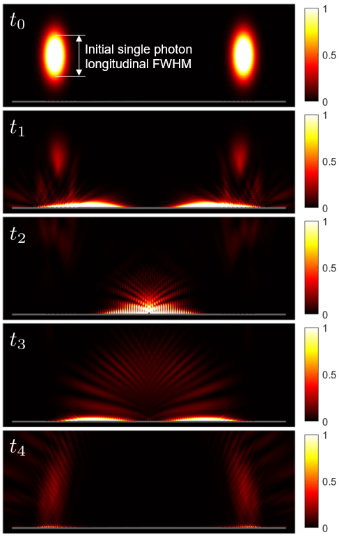
Figure 4: The magnitude of $\matrixelement{\Psi^{(2)}_{t_{0}}}{\hat{\mathbf{E}}^{(-)}(\mathbf{r},t)\cdot\hat{\mathbf{E}}^{(+)}(\mathbf{r},t)}{\Psi^{(2)}_{t_{0}}}$ at different time lapses $t=t_{0},t_{1},t_{2},t_{3},t_{4}$ in the presence of the plasmonic beam splitter.

Fig. 5 shows second-order correlations versus $\tau$ for three cases: (i) with the plasmonic BS and coincidence of out-coupled free fields, (ii) with the plasmonic BS and coincidence of SPP fields, and (iii) with coincidence of out-coupled free fields in the absence of the plasmonic BS. It can be clearly observed in the cases (i) and (ii) that the HOM dip exists when $\tau$ is small (around the longitudinal FWHM of the initial single photon) whereas the case (iii) yields the almost unity second-order correlation. This is because the plasmonic BS gives rise to the destructive interference between two SPPs. Not exactly zeroing at $\tau=0$ is due to the gold loss and imperfect destructive interference due to the the narrow bandwidth characteristics of the plasmonic BS 50:50 performance. It is interesting to compare the cases (i) and (ii) that the case (ii) has the slightly narrower full-width half maximum (FWHM) width (i.e., the higher quality factor) in the HOM curve compared with the case (i). This is because of the SPP-propagation dispersion effects and degradations of the out-coupling process are accounted in the case (i). Note that the evaluation of second order correlations from the coincidence of bosonic particles contained in SPP fields is only allowed in numerical simulations due to limitations of experimental setups. The maturation of quantum information science technology will bring about the integration of circuits. As a result, fully quantum-theoretic numerical simulations are expected to be much more important. Through numerical experiments, in principle, one can do direct observations of arbitrary quantum phenomena, which is challenging in real experiments. For example, our recent works that developed full-wave numerical solvers for the macroscopic circuit QED [20, 21] are greatly helpful for the design of quantum information processing hardware based on superconducting circuits and transmon qubits. Likewise, the present numerical framework will enable quantitative evaluations of open and dissipative quantum optics problems involving arbitrary medium inhomogeneity and geometric complexity.

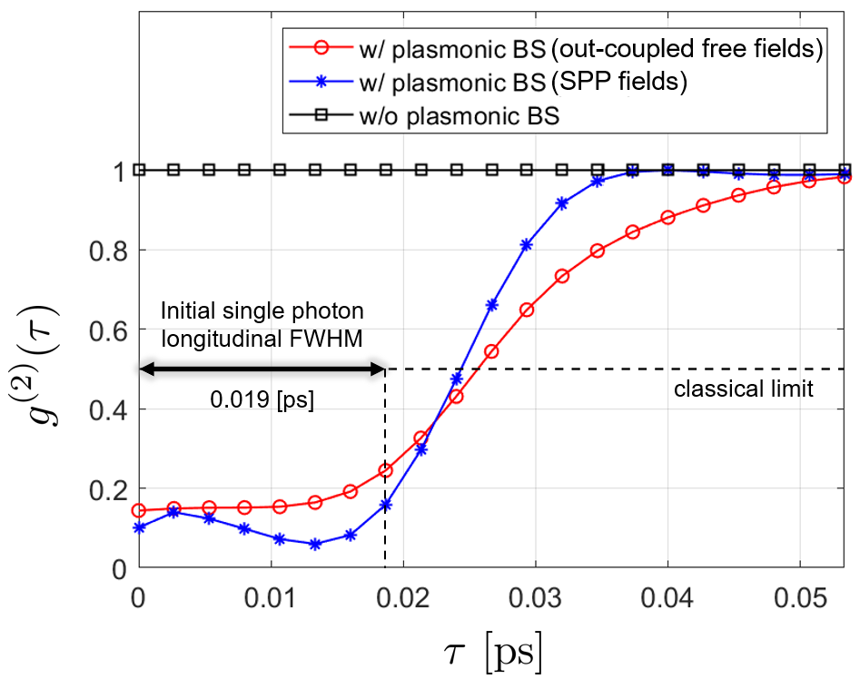
Figure 5: Second order correlation versus $\tau$ for three cases: (i) with the plasmonic beam splitter and coincidence of out-coupled free fields, (ii) with the plasmonic beam splitter and coincidence of surface plasmon polariton fields, and (iii) with coincidence of out-coupled free fields in the absence of the plasmonic beam splitter.

The future works will focus on validating and extending the present numerical framework for the new LN formalism. First, we will connect the new LN formalism to the explicit model [22, 23, 1] with the use of numerical diagonalization methods [24, 25]. Second, we will also explore the use of integral-equation or time-domain CEM solvers which potentially reduce the computational loads further to find BAMA fields. Finally, we will apply the present numerical framework to studying a variety of quantum optics applications, such as, modeling metasurface-based quantum optics devices and ultrafast single-photon sources based on a nitrogen-vacancy center in a diamond coupled to plasmonic nanostructures.

References

-
[1]
A. Drezet,
Quantizing
polaritons in inhomogeneous dissipative systems, Phys. Rev. A 95 (2017)
023831.
doi:10.1103/PhysRevA.95.023831.
URL https://link.aps.org/doi/10.1103/PhysRevA.95.023831 -
[2]
O. D. Stefano, S. Savasta, R. Girlanda,
Mode expansion and photon
operators in dispersive and absorbing dielectrics, Journal of Modern Optics
48 (1) (2001) 67–84.
arXiv:https://doi.org/10.1080/09500340108235155, doi:10.1080/09500340108235155.
URL https://doi.org/10.1080/09500340108235155 -
[3]
G. Di Martino, Y. Sonnefraud, M. S. Tame, S. Kéna-Cohen, F. Dieleman, i. m.
c. K. Özdemir, M. S. Kim, S. A. Maier,
Observation
of quantum interference in the plasmonic hong-ou-mandel effect, Phys. Rev.
Applied 1 (2014) 034004.
doi:10.1103/PhysRevApplied.1.034004.
URL https://link.aps.org/doi/10.1103/PhysRevApplied.1.034004 -
[4]
M.-C. Dheur, E. Devaux, T. W. Ebbesen, A. Baron, J.-C. Rodier, J.-P. Hugonin,
P. Lalanne, J.-J. Greffet, G. Messin, F. Marquier,
Single-plasmon
interferences, Science Advances 2 (3) (2016) e1501574.
arXiv:https://www.science.org/doi/pdf/10.1126/sciadv.1501574, doi:10.1126/sciadv.1501574.
URL https://www.science.org/doi/abs/10.1126/sciadv.1501574 -
[5]
B. Vest, M.-C. Dheur, Éloïse Devaux, A. Baron, E. Rousseau, J.-P. Hugonin,
J.-J. Greffet, G. Messin, F. Marquier,
Anti-coalescence
of bosons on a lossy beam splitter, Science 356 (6345) (2017) 1373–1376.
arXiv:https://www.science.org/doi/pdf/10.1126/science.aam9353, doi:10.1126/science.aam9353.
URL https://www.science.org/doi/abs/10.1126/science.aam9353 - [6] C. K. Hong, Z. Y. Ou, L. Mandel, Measurement of subpicosecond time intervals between two photons by interference, Phys. Rev. Lett. 59 (1987) 2044–2046.
- [7] R. J. Glauber, M. Lewenstein, Quantum optics of dielectric media, Phys. Rev. A 43 (1991) 467–491.
- [8] M. O. Scully, M. S. Zubairy, Quantum Optics, American Association of Physics Teachers (AAPT), College Park, MD, USA, 1999.
- [9] W. C. Chew, A. Y. Liu, C. Salazar-Lazaro, W. E. I. Sha, Quantum electromagnetics: A new look-Part I and Part II, J. Multiscale and Multiphys. Comput. Techn. 1 (2016) 73–97.
- [10] D.-Y. Na, J. Zhu, W. C. Chew, F. L. Teixeira, Quantum information preserving computational electromagnetics, Phys. Rev. A 102 (2020) 013711.
-
[11]
T. Gruner, D.-G. Welsch,
Green-function
approach to the radiation-field quantization for homogeneous and
inhomogeneous kramers-kronig dielectrics, Phys. Rev. A 53 (1996) 1818–1829.
doi:10.1103/PhysRevA.53.1818.
URL https://link.aps.org/doi/10.1103/PhysRevA.53.1818 - [12] H. T. Dung, L. Knöll, D.-G. Welsch, Three-dimensional quantization of the electromagnetic field in dispersive and absorbing inhomogeneous dielectrics, Phys. Rev. A 57 (1998) 3931–3942.
- [13] J. Jin, The Finite Element Method in Electromagnetics, 3rd Edition, Wiley-IEEE Press, 2014.
-
[14]
A. Bossavit,
Whitney
forms: a class of finite elements for three-dimensional computations in
electromagnetism, IEE Proceedings A (Physical Science, Measurement and
Instrumentation, Management and Education, Reviews) 135 (1988) 493–500(7).
URL https://digital-library.theiet.org/content/journals/10.1049/ip-a-1.1988.0077 - [15] H. H. Gan, Q. I. Dai, T. Xia, W. C. Chew, C.-F. Wang, Broadband spectral numerical green’s function for electromagnetic analysis of inhomogeneous objects, IEEE Antennas and Wireless Propagation Letters 19 (7) (2020) 1063–1067. doi:10.1109/LAWP.2020.2988475.
-
[16]
A. Baron, E. Devaux, J.-C. Rodier, J.-P. Hugonin, E. Rousseau, C. Genet, T. W.
Ebbesen, P. Lalanne, Compact antenna
for efficient and unidirectional launching and decoupling of surface
plasmons, Nano Letters 11 (10) (2011) 4207–4212.
doi:10.1021/nl202135w.
URL https://doi.org/10.1021/nl202135w -
[17]
K. M. McPeak, S. V. Jayanti, S. J. P. Kress, S. Meyer, S. Iotti, A. Rossinelli,
D. J. Norris, Plasmonic films can
easily be better: Rules and recipes, ACS Photonics 2 (3) (2015) 326–333.
doi:10.1021/ph5004237.
URL https://doi.org/10.1021/ph5004237 - [18] L. Mandel, E. Wolf, Optical Coherence and Quantum Optics, Cambridge University Press, Cambridge, UK, 1995.
-
[19]
S. Scheel, S. Y. Buhmann, Macroscopic
qed - concepts and applications (2009).
doi:10.48550/ARXIV.0902.3586.
URL https://arxiv.org/abs/0902.3586 - [20] T. E. Roth, W. C. Chew, Macroscopic circuit quantum electrodynamics: A new look toward developing full-wave numerical models, IEEE Journal on Multiscale and Multiphysics Computational Techniques 6 (2021) 109–124. doi:10.1109/JMMCT.2021.3112808.
-
[21]
T. E. Roth, W. C. Chew, Full-wave
methodology to compute the spontaneous emission rate of a transmon qubit
(2022).
doi:10.48550/ARXIV.2201.04244.
URL https://arxiv.org/abs/2201.04244 - [22] T. G. Philbin, Canonical quantization of macroscopic electromagnetism, New J. Phys. 12 (12) (2010) 123008.
- [23] W. E. I. Sha, A. Y. Liu, W. C. Chew, Dissipative quantum electromagnetics, J. Multiscale and Multiphys. Comput. Techn. 3 (2018) 198–213.
-
[24]
V. Dorier, J. Lampart, S. Guérin, H. R. Jauslin,
Canonical
quantization for quantum plasmonics with finite nanostructures, Phys. Rev. A
100 (2019) 042111.
doi:10.1103/PhysRevA.100.042111.
URL https://link.aps.org/doi/10.1103/PhysRevA.100.042111 -
[25]
D.-Y. Na, J. Zhu, W. C. Chew,
Diagonalization
of the hamiltonian for finite-sized dispersive media: Canonical quantization
with numerical mode decomposition, Phys. Rev. A 103 (2021) 063707.
doi:10.1103/PhysRevA.103.063707.
URL https://link.aps.org/doi/10.1103/PhysRevA.103.063707