Valley-magnetophonon resonance for interlayer excitons

Abstract

Heterobilayers consisting of MoSe₂ and WSe₂ monolayers can host optically bright interlayer excitons with intriguing properties such as ultralong lifetimes and pronounced circular polarization of their photoluminescence due to valley polarization, which can be induced by circularly polarized excitation or applied magnetic fields. Here, we report on the observation of an intrinsic valley-magnetophonon resonance for localized interlayer excitons promoted by invervalley hole scattering. It leads to a resonant increase of the photoluminescence polarization degree at the same field of 24.2 Tesla for H-type and R-type stacking configurations despite their vastly different excitonic energy splittings. As a microscopic mechanism of the hole intervalley scattering we identify the scattering with chiral TA phonons of MoSe₂ between excitonic states mixed by the long-range electron hole exchange interaction.

I Introduction

Two-dimensional (2D) crystals and their van der Waals (vdW) heterostructures (HS) are promising candidates for novel optoelectronic devices. Among the 2D crystals, the semiconducting transition metal dichalcogenides (TMDCs) like MoS₂ have garnered a lot of attention due their intriguing properties: in the monolayer (ML) limit, they are direct-gap semiconductors Mak et al. (2010); Splendiani et al. (2010) with large exciton binding energies Chernikov et al. (2014) and peculiarities such as spin-valley locking Xiao et al. (2012). The latter phenomenon, coupled with helicity-dependent interband selection rules, allows for optical initialization and readout of a coupled spin-valley polarization Xu et al. (2014). Many combinations of different TMDC MLs yield a type-II band alignment, which leads to interlayer charge separation. Spatially separated electron-hole pairs can form so-called interlayer excitons (ILE) in these heterobilayers Rivera et al. (2018). Depending on the specific material combination, these ILE may be optically bright only for specific crystallographic alignments Nayak et al. (2017) (interlayer twist) and their energy may be tunable via control of interlayer twist Kunstmann et al. (2018); Tebyetekerwa et al. (2021). These ILE inherit some properties, such as spin-valley polarization Rivera et al. (2016), from the constituent TMDC MLs. However, in contrast to monolayer excitons, they are characterized by ultralong lifetimes Rivera et al. (2015); Miller et al. (2017); Nagler et al. (2017a) and diffusion over mesoscopic distances Rivera et al. (2016); Unuchek et al. (2018), which makes them attractive for exciton-based optoelectronic devices, see Ref. Ciarrocchi et al., 2022 for a recent review.

Magneto-optical studies in high magnetic fields have been used very successfully to elucidate properties of TMDC monolayers, such as exciton g factors MacNeill et al. (2015), magnetic-field-induced valley polarization Mitioglu et al. (2015), exciton Bohr radii and masses Stier et al. (2016); Goryca et al. (2019), dark exciton Zhang, Xiao-Xiao et al. (2017) and Rydberg exciton states Stier et al. (2018); Wang et al. (2020), as well as the substructure of more complex quasiparticles like biexcitons Nagler et al. (2018); Barbone et al. (2018); Li et al. (2018), see also Ref. Arora, 2021 for a recent review. More recently, ILE in TMDC heterobilayers have also been subjected to high magnetic fields, revealing a unique ability to engineer their effective g factor by changing the twist angle Nagler et al. (2017b), which can obtain values far larger than those observed in TMDC ML excitons or change its sign Ciarrocchi et al. (2019); Seyler et al. (2019).

For the specific material combination of WSe₂ and MoSe₂, optically bright ILE are only observable for interlayer twist angles close to 0 or 60 degrees Nayak et al. (2017). These configurations are also referred to as R-type (0 degree) or H-type (60 degree) in accordance to the prevalent stacking polymorphs of TMDC multilayers. The optical selection rules for ILE in these structures depend on the local interlayer atomic registry Yu et al. (2017), and therefore, the helicity of the emitted PL is not directly linked to ILE valley polarization, in contrast to TMDC monolayers. In heterobilayers, the interlayer atomic registry can vary spatially due to two different effects:

• the formation of a moiré lattice Seyler et al. (2019); Tran et al. (2019), which arises from an angular misalignment of the individual layers.

• atomic reconstruction Rosenberger et al. (2020); Weston et al. (2020), in which the individual layers are slightly distorted to yield domains with perfect interlayer atomic registry separated by domain walls.

Both effects lead to exciton localization, which can be used to study highly tunable manybody phases of excitons and individual charge carriers Yu et al. (2017); Brotons-Gisbert et al. (2020); Shabani et al. (2021); Zhang et al. (2021) .

In two independent magneto-optical studies on ILE in H-type structures Nagler et al. (2017b); Delhomme et al. (2020), a peculiar enhancement of ILE valley polarization was found in magnetic fields of about 24 Tesla. In the latter study, this enhancement was associated with a coupling between ILE and chiral optical phonons Ribeiro-Soares et al. (2014); Zhang and Niu (2015); He et al. (2020). The strong electron-phonon and exciton-phonon interactions were also shown to limit the mobility Kaasbjerg et al. (2012); Song and Dery (2013); Li et al. (2013); Jin et al. (2014), lead to formation of polarons Christiansen et al. (2017); Li and Wang (2018); Chen et al. (2018); Glazov et al. (2019), and produce phonon cascades Chow et al. (2017); Shree et al. (2018); Brem et al. (2018); Paradisanos et al. (2021).

Here, we present a joint experimental and theoretical study of ILE in both H-type and R-type WSe₂-MoSe₂ heterobilayers. In magneto-photoluminescence measurements, we observe a pronounced enhancement of the ILE valley polarization at about 24.2 Tesla for both types of structure, even though their g factors, and the corresponding valley Zeeman splitting of the ILE, differ by about a factor of 3. This observation is explained as a valley-magnetophonon resonance of a hole in the localized exciton. Our theoretical analysis reveals the dominant mechanism of the valley-magnetophonon resonance to be electron-spin-conserving scattering with a chiral TA phonon originating from MoSe₂ ML between the excitonic states mixed by the long-range exchange interaction.

The magnetophonon resonance was predicted more than half a century ago by V. L. Gurevich and Yu. A. Firsov Gurevich and Firsov (1961) as an intrinsic resonance between a pair of Landau levels and the optical phonon energy. Soon after, the spin-magnetophonon resonance between opposite electron spin states was predicted Pavlov et al. (1965) and observed Aksel’rod and Tsidil’kovskii (1966). Spin-conserving intervalley magnetophonon resonances were also studied in conventional semiconductors Firsov et al. (1991), graphene Basko et al. (2016) and TMDC MLs Glazov et al. (2019). Eventually the magnetophonon resonance evolved into a powerful tool to study both the phonon and electron properties of metals, semiconductors and semiconductor nanostructures Firsov et al. (1991); Langerak et al. (1988); Barnes et al. (1991); Vaughan et al. (1996). However, despite numerous investigations and applications of the magnetophonon resonance, an intervalley spin-flip resonance was never observed before to the best of our knowledge. Thus the hole valley-magnetophonon resonance represents a novel aspect of this tool highly relevant for TMDC HS.

II Experimental results

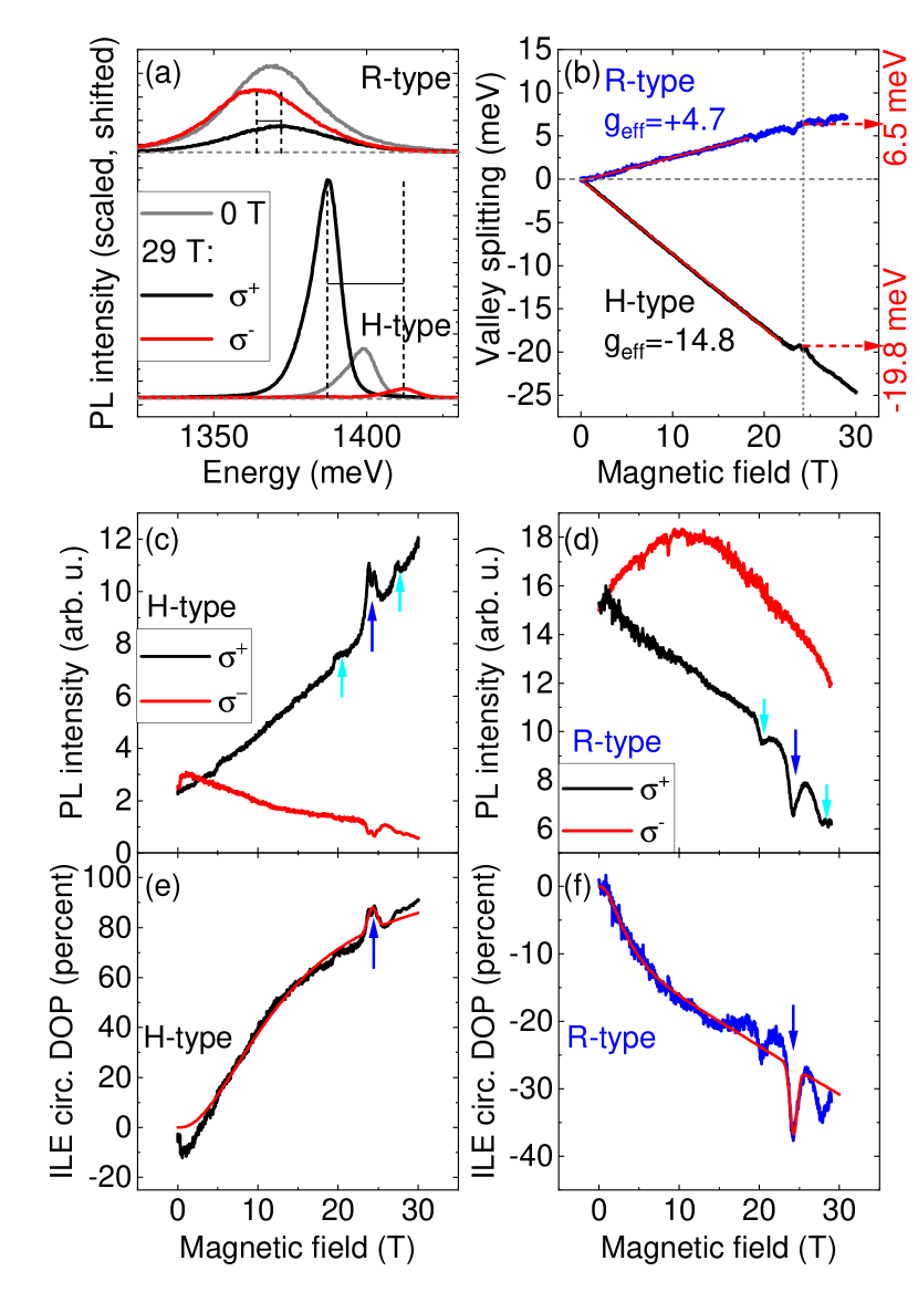
Figure 1: (a) PL spectra of R-type and H-type HS at 0 T (grey lines) and helicity-resolved PL spectra at 29 T. The vertical dashed lines indicate the splitting between $\sigma^{+}$ and $\sigma^{-}$ emission at 29 T. (b) Valley splitting in R-type (blue line) and H-type (black line) HS as a function of magnetic field. The red lines indicate linear fits to the data. The vertical dashed line indicates the resonance field of 24.2 T. The red arrows indicate the valley splitting values for the different HS at this field. (c+d) Helicity-resolved PL intensity for H-type (c) and R-type (d) HS as a function of magnetic field. The blue arrows indicate the resonantly increased (c) / decreased (d) PL intensity at the resonance field. The light blue arrows indicate the weaker resonant features. (e+f) ILE PL circular degree of polarization for H-type (e) and R-type (f) HS calculated from data in (c+d). The red solid lines in (e) and (f) indicate fits to the data using our model. Blue arrows indicate the resonantly enhanced degree of polarization.

Our results are summarized in Fig. 1. ILE in H-type and R-type heterobilayers are directly distinguishable by their emission energy and spectral linewidth, even in zero-field photoluminescence (PL) spectra Holler et al. (2022). As Fig. 1(a) shows, at 0 Tesla the ILE in the H-type structure has its emission peak at around 1399 meV, with a linewidth of about 13 meV. By contrast, the ILE in R-type structure emits at the significantly lower energy of about 1368 meV and has a larger linewidth of about 37 meV. In a high magnetic field (29 Tesla spectra are depicted in Fig. 1(a)), helicity-resolved PL spectra reveal a pronounced energetic splitting of $\sigma^{+}$ and $\sigma^{-}$ polarized emission, combined with a pronounced change in relative emission intensities. For both H-type and R-type ILE, the lower-energy emission becomes more intense than the high-energy emission. However, for the two structures, $\sigma^{+}$ and $\sigma^{-}$ components shift in opposite ways: for H-type, the $\sigma^{-}$ component shifts to higher energy, while for R-type, it is the $\sigma^{+}$ component. It is also directly evident that the magnitude of the field-induced shifts is far larger in the H-type ILE. In order to quantify these observations, we performed continuous sweeps of the magnetic field from 0 T to 30 T (H-type) or 29 T(R-type), with helicity-resolved PL spectra taken at fixed time intervals corresponding to about 27 mT spacing between spectra. For each spectrum, the ILE signal was analyzed using an automatized Gaussian fit routine to extract its peak position and integrated intensity. From these datasets, we were able to determine the dependence of the valley splitting $\Delta E$ (defined as $\Delta E=E_{\sigma^{+}}-E_{\sigma^{-}})$ on magnetic field, as depicted in Fig. 1(b). We clearly see a linear dependence for both types of ILE, with opposite sign and different slope. A linear fit yields the effective ILE g factors of $g_{eff}$=-14.8 for the H-type and $g_{eff}$=+4.7 for the R-type structure. Close to the resonance field of 24.2 T, we note a slight deviation of the measured valley splitting from the linear behavior for both structures. Noteworthy, the valley splitting at this resonance field differs by a factor of more than 3 between the structures, as indicated by the red arrows.

In addition to the valley-selective shifting of ILE energies, the magnetic field also modifies the relative intensities of $\sigma^{+}$ and $\sigma^{-}$ emission. We plot the helicity-resolved integrated PL intensities as a function of magnetic field for both structures in Fig. 1(c) (H-type) and (d) (R-type), respectively. For the H-type ILE, the $\sigma^{+}$ emission increases almost monotonously with magnetic field, while $\sigma^{-}$ decreases almost monotonously. However, we note a pronounced, resonant increase of the $\sigma^{+}$ emission at the resonance field of 24.2 T (marked by blue arrow). In the H-type structure, this is accompanied by a resonant reduction of the $\sigma^{-}$ emission at the same field. By contrast, in the R-type structure, the $\sigma^{-}$ initially increases up to about 10 T, then decreases. The $\sigma^{+}$ emission decreases almost monotonously, but we notice a pronounced, resonant decrease at the resonance field (marked by blue arrow). In the R-type structure, this is not accompanied by an increased emission in the opposite helicity. Looking more closely, we also see two weaker resonant features for both structures at fields slightly above and below the resonance field (marked by light blue arrows).

From these datasets, we calculate the circular degree of polarization (DOP) of the ILE emission, defined as

$$\text{DOP}=\frac{I^{\sigma^{+}}-I^{\sigma^{-}}}{I^{\sigma^{+}}+I^{\sigma^{-}}}$$ (1)

with the helicity-resolved PL intensities $I^{\sigma^{+}}$ and $I^{\sigma^{-}}$. The DOP as a function of magnetic field is depicted in Fig. 1(e) and (f). We note that, based on our definition, it is positive for the H-type structure and negative for the R-type structure. For both ILE types, the absolute value of the DOP increases as a function of magnetic field. In both cases, we clearly see a resonantly increased absolute value of the DOP at the resonance field, accompanied by two additional, weaker resonant features below and above the main resonance. While the DOP for the H-type structure reaches near-unity values above 90 percent at the largest applied magnetic field, the maximum absolute value for the R-type structure is lower at about 37 percent and actually achieved at the resonance field. This difference in the maximum DOP closely corresponds to the difference of the valley splittings.

Our most surprising observation is the resonant enhancement of the DOP at the same field of 24.2 T despite the large difference of the valley splittings. Below, we demonstrate that this is a consequence of the hole valley-magnetophonon resonance.

III Theory

The effective exciton g factors for H-type and R-type HS and bright PL agree with the dominant contribution of H${}_{h}^{h}$ (AA^′) Nagler et al. (2017b); Zhang et al. (2019); Brotons-Gisbert et al. (2020) and R${}_{h}^{X}$ (A^′B^′) Ciarrocchi et al. (2019); Joe et al. (2021) interlayer atomic registries to the optical properties in agreement with the previous studies of MoSe₂/WSe₂ HS. These g factors stem from the individual electron and hole g factors as $-g_{e}\mp g_{h}$, respectively, where “hole” refers to the vacant state in the valence band. From the measured values of $-14.8$ and $+4.7$ we estimate the electron and hole g factors to be $g_{e}=5.05$ and $g_{h}=9.75$ in agreement with first principle calculations Woźniak et al. (2020); Xuan and Quek (2020); Deilmann et al. (2020); Förste et al. (2020).

The resonant changes of the PL at the same magnetic field $B_{\text{res}}=24.2$ T in both H-type and R-type HS suggest a common resonance. Despite the large difference in the exciton valley splittings the individual electron and hole Zeeman energies are the same at the given magnetic field for both stacking configurations. Therefore we attribute the observed resonances to the individual charge carriers.

Electron or hole intervalley scattering requires a spin flip and absorption or emission of a chiral phonon at the corner of the Brillouin zone (K points). The large density of chiral phonon states strongly increases the scattering rate. Due to the spin-valley locking the observed resonance represents a spin-valley magnetophonon resonance. Intervalley spin-magnetophonon resonances were never observed before to the best of our knowledge.

The electron and hole Zeeman splittings in the field $B_{\text{res}}$ are $g_{e}\mu_{B}B_{\text{res}}=7.1$ meV and $g_{h}\mu_{B}B_{\text{res}}=13.7$ meV. Calculations of the phonon energies in MoSe₂ and WSe₂ Song and Dery (2013); Horzum et al. (2013); Huang et al. (2013); Peng et al. (2016); Lin et al. (2021a, b) demonstrate the absence of K phonon modes at the Zeeman splitting of the electron. However in the vicinity of the hole Zeeman splitting there are the chiral ZA phonon mode of WSe₂ at $15$ meV and the chiral TA phonon mode of MoSe₂ at $14.7$ meV. Taking into account the possible phonon energy renormalization Mahrouche et al. (2022); Parzefall et al. (2021) we conclude that we observe a valley-magnetophonon resonance of a hole.

III.1 Valley magnetophonon resonance in PL polarization

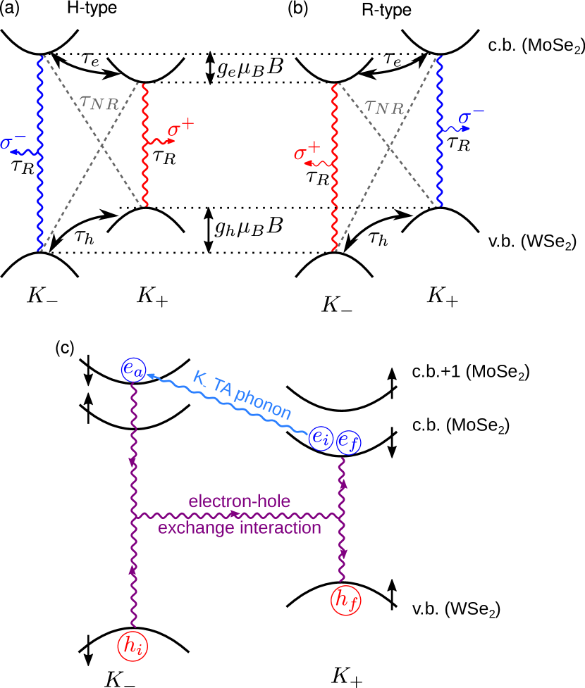
Figure 2: (a,b) Optical selection rules in H${}_{h}^{h}$ (a) and R${}_{h}^{X}$ (b) interlayer atomic registries of MoSe₂/WSe₂ HS, electron ($\tau_{e}$) and hole ($\tau_{h}$) intervalley scatterings, radiative ($\tau_{R}$) and nonradiative ($\tau_{NR}$) electron hole recombinations, and Zeeman splittings of the conduction ($g_{e}\mu_{B}B$) and valence ($g_{h}\mu_{B}B$) bands. (c) Two step hole intervalley scattering involving electron-spin-conserving intervalley scattering with chiral TA phonon and exciton intervalley mixing by the long range exchange interaction. The electron and hole states are denoted as $e_{i}$, $h_{i}$ (initial), $e_{a}$ (auxiliary), and $e_{f}$, $h_{f}$ (final). The Zeeman splittings and spin states (black arrows) correspond to H-type HS.

In order to demonstrate that the hole valley magnetophonon resonance leads to the resonant enhancement of the PL polarization we consider the exciton spin dynamics using rate equations for the four lowest intravalley and intervalley excitonic states shown in Fig. 2(a,b) SI . We take into account radiative and nonradiative exciton recombination times, $\tau_{R}$ and $\tau_{NR}$, respectively, as well as the electron, $\tau_{e}(B)$, and hole, $\tau_{h}(B)$, intervalley scattering times to the lower energy states. Note that the actual hole scattering mechanism may be quite complex and involve both charge carriers in a single scattering event, as shown in the next subsection. The scattering times to the higher energy states are larger by the corresponding factors $\exp(g_{e,h}\mu_{B}B/k_{B}T)$ with $T$ being the temperature and $k_{B}$ being the Boltzmann constant.

For the hole valley relaxation time we assume the following form:

$$\frac{1}{\tau_{h}(B)}=\frac{1}{\tau_{\text{res}}}\exp\left[-\frac{(B-B_{\text{res}})^{2}}{\Delta B^{2}}\right]+\frac{1}{\tau_{h}^{(0)}}\left(\frac{B}{B_{\text{res}}}\right)^{2}.$$ (2)

Here the first term stands for the resonant intervalley scattering at field $B_{\text{res}}$ with the minimum time $\tau_{\text{res}}$ and the width of the resonance $\Delta B$. The second term describes the phenomenological scattering time $\tau_{h}(B)\propto 1/B^{2}$, which corresponds to the direct spin-phonon coupling in strained HS in small magnetic fields Pearce and Burkard (2017). Similarly to this, for the electron intervalley scattering we assume $\tau_{e}(B)=\tau_{e}^{(0)}(B_{\text{res}}/B)^{2}$.

Figure 1(e,f) shows that this model nicely fits the polarization degree of PL almost in the whole range of magnetic fields from 0 to 29 T including the resonant enhancement at 24.2 T. The fit parameters are given and discussed in the Supplementary material SI . The surprisingly good quality of the fit demonstrates that the resonant enhancement of the PL polarization degree is related to the valley-magnetophonon resonance.

III.2 Mechanism of hole valley-magnetophonon resonance

Direct intervalley scattering between Kramers degenerate states of the hole is forbidden by the time reversal symmetry Bir and Pikus (1974); Ivchenko et al. (1990); Song and Dery (2013). However, it becomes possible in the presence of the external magnetic field Khaetskii and Nazarov (2001) or hole-electron exchange interaction Tsitsishvili et al. (2003). The excitons in our MoSe₂/WSe₂ HS are localized either due to the moiré potential or the domains formed by atomic reconstruction. We find that the dominant mechanism of the hole valley-magnetophonon resonance in this case is a two step process SI , as illustrated in Fig. 2(c). To be specific, let us consider the scattering from an intervalley excitonic state with longer lifetime to an intravalley state with a short lifetime with the transition of a hole in exciton to a state with lower energy at the $K_{+}$ valley, as shown in Fig. 2(c). At the first step, an electron from the $K_{+}$ valley virtually scatters to the upper (spin split) subband in the $K_{-}$ valley emitting a chiral TA phonon of the MoSe₂ ML. The phonon emission ensures the energy conservation for the entire two-step scattering, and the intermediate (auxiliary) exciton state has a very short lifetime limited by the time-energy uncertainty relation. At the second step the exciton scatters as a whole from the $K_{-}$ valley to the ground state in the $K_{+}$ valley due to the long-range electron hole exchange interaction. This step can be described as emission and reabsorption of a virtual longitudinal photon Bir and Pikus (1974); Goupalov et al. (2003); Glazov et al. (2014). The efficiency of this scattering is ensured by the brightened spin-triplet exciton states and specific optical selection rules for H${}_{h}^{h}$ and R${}_{h}^{X}$ interlayer atomic registries Yu et al. (2018). In total, the electron remains in the same state, and the hole flips its valley. The hole scattering from intravalley exciton state in $K_{-}$ to $K_{+}$ valley has the same rate, and the scattering with increase of the energy is suppressed by the Boltzmann factor.

The scattering rate is given by the Fermi’s golden rule

$$\frac{1}{\tau_{\text{res}}}=\frac{2\pi}{\hbar}\sum_{\bm{q}}\left|\frac{\left<f_{\bm{q}}\middle|\mathcal{H}_{\text{exch}}\middle|a_{\bm{q}}\right>\left<a_{\bm{q}}\middle|\mathcal{H}_{\text{e-ph}}\middle|i\right>}{E_{f}-E_{a}}\right|^{2}\delta(E_{i}-E_{f}-\hbar\Omega_{q}),$$ (3)

where $i$, $a_{\bm{q}}$, $f_{\bm{q}}$ represent the initial, auxiliary and final states of exciton and emitted phonon with the wave vector $\bm{K}_{-}+\bm{q}$ and energy $\hbar\Omega_{q}$, $E_{i,a,f}$ are the exciton energies in the corresponding states, and $\mathcal{H}_{\text{exch}}$ and $\mathcal{H}_{\text{e-ph}}$ stand for the exchange and electron-phonon interaction Hamiltonians. In the vicinity of the magnetophonon resonance one has $E_{a}-E_{f}=\Delta_{c}+(g_{h}-g_{e}^{v})\mu_{B}B_{\text{res}}$, where $\Delta_{c}$ is the spin orbit splitting of MoSe₂ conduction band and $g_{e}^{v}$ is the electron valley g factor Wang et al. (2015); Durnev and Glazov (2018).

From the symmetry analysis we find that the electron interaction with chiral TA phonons in MoSe₂ ML is described by SI

$$\mathcal{H}_{\text{e-ph}}=\sum_{\bm{q},\pm}\sqrt{\frac{\hbar}{2\rho\Omega_{q}A}}\Xi q_{\pm}{\hat{\tau}_{\pm}}b_{\bm{K}_{\pm}+\bm{q}}^{\dagger}\mathrm{e}^{-\mathrm{i}\bm{q}\bm{r}_{e}}+{\text{H.c.}},$$ (4)

where $b_{\bm{k}}^{\dagger}$ are the phonon creation operators, $\rho$ is two-dimensional mass density of the ML, $A$ is the normalization area, $q_{\pm}=(q_{x}\pm\mathrm{i}q_{y})/\sqrt{2}$, $\Xi$ is the intervalley deformation potential, $\bm{r}_{e}$ is the electron coordinate, and ${\hat{\tau}_{\pm}}$ are the electron valley rising and lowering operators, which conserve the electron spin. This Hamiltonian can be derived taking into account that electrons and phonons at $K_{\pm}$ valleys have orbital angular momenta $\pm 1$ and $\mp 1$, respectively, and that the angular momentum modulo 3 should be conserved during the scattering. The phonon dispersion at the corners of the Brillouin zone has the form $\hbar\Omega_{q}=\hbar\Omega_{0}+(\hbar q)^{2}/(2M)$ Peng et al. (2016), where $M$ is the effective phonon mass at $K$ point.

The Hamiltonian of the long-range exchange interaction between auxiliary and final states can be obtained similarly to the ML case Glazov et al. (2014), it reads

$$\mathcal{H}_{\text{exch}}=\frac{2\pi e^{2}\delta(\bm{\rho})}{\varkappa_{b}m_{0}^{2}\omega_{0}^{2}}\frac{(\bm{K}\bm{p}_{\text{c.v.}}^{a})(\bm{K}\bm{p}_{\text{c.v.}}^{f})^{*}}{K},$$ (5)

where $\bm{\rho}$ is the distance between electron and hole, $\varkappa_{b}$ is the background dielectric constant, $m_{0}$ is the free electron mass, $\omega_{0}$ is the exciton resonance frequency, $\bm{K}$ is the exciton center of mass momentum, and $p_{c.v.}^{a,f}$ are the interband momentum matrix elements for the auxiliary and final states.

To calculate the scattering rate we consider the wave function of the localized exciton $\propto\mathrm{e}^{-\rho/a_{B}-R^{2}/(2l^{2})}$, where $a_{B}$ and $l$ are the exciton Bohr radius and the localization length, and $\bm{R}$ is the exciton center of mass coordinate. Then under assumption of the low temperature, $k_{B}T\ll g_{h}\mu_{B}B_{\text{res}}$ we obtain the hole intervalley scattering rate SI

$$\frac{1}{\tau_{\text{res}}}=\frac{\pi mM^{2}\Gamma_{0}^{a}\Gamma_{0}^{f}E_{\text{loc}}\Xi^{2}(B-B_{\text{res}})}{4\hbar^{3}\rho k^{2}\left(E_{a}-E_{f}\right)^{2}B_{\text{res}}}\theta(B-B_{\text{res}})\\ \times\exp\left(-\frac{Mg_{h}\mu_{B}(B-B_{\text{res}})}{mE_{\text{loc}}}\right),$$ (6)

where $E_{\text{loc}}=\hbar^{2}/(ml^{2})$ is the exciton localization energy with $m$ being the exciton mass and $\Gamma_{0}^{a,f}=2\pi k^{2}e^{2}|p_{\text{c.v.}}^{a,f}|^{2}|\varphi(0)|^{2}/(\hbar\varkappa_{b}\omega_{0}^{2}m_{0}^{2})$ are the free exciton radiative decay rates in the auxiliary and final states with $\varphi(0)=\sqrt{2/\pi}/a_{B}$ being the wave function of the relative electron hole motion at $\rho=0$ and $k=\sqrt{\varkappa_{b}}\omega_{0}/c$ being the light wave vector.

One can see that the hole intervalley scattering rate vanishes at magnetic fields below $B_{\text{res}}$, as there are no phonons of the required energy, which is described by the Heaviside step function $\theta(B-B_{\text{res}})$. Just above $B_{\text{res}}$ the scattering rate grows linearly with increase of $B-B_{\text{res}}$ because of the increase of the electron-phonon interaction matrix element. However at high magnetic fields the exciton-phonon matrix element decreases exponentially because of the exciton localization. As a result, the hole intervalley scattering rate has a narrow maximum at $B\approx B_{\text{res}}$ with the width of the order of $mE_{\text{loc}}/(g_{h}\mu_{B}M)$. In the maximum it reaches

$$\frac{1}{\tau_{\text{res}}}=\frac{\pi m^{2}M\Gamma_{0}^{a}\Gamma_{0}^{f}E_{\text{loc}}^{2}\Xi^{2}}{4\hbar^{3}\rho k^{2}(E_{a}-E_{f})^{2}g_{h}\mu_{B}B_{\text{res}}}.$$ (7)

Substitution of the material parameters yields SI $\tau_{\text{res}}=12$ ns and $20$ ns for H-type and R-type HS, which agrees with the timescales of the PL polarization saturation Holler et al. (2022).

IV Discussion and conclusion

The resonant increase of the PL polarization in the same magnetic field for H-type and R-type HS unambiguously reveals a valley-magnetophonon resonance. The weaker resonance below and higher by approximately 3.8 T for both HS may be related to some combined phonon resonances, but their exact nature is not completely clear.

The dominant microscopic mechanism of the hole valley-magnetophonon resonance is found to be the scattering with chiral TA phonon of MoSe₂ between the excitonic states mixed by the long-range exchange interaction. Noteworthy it has a few solid advantages: (i) it does not require spin-dependent electron-phonon interaction, (ii) it profits from the large density of chiral phonon states, (iii) it is free of the Van Vleck cancellation, (iv) the long-range exchange interaction is enhanced by the exciton localization, and (v) optical selection rules for excitons in H${}_{h}^{h}$ and $R_{h}^{X}$ atomic registries exactly match the requirements for the exchange interaction. The unique observation of the valley-magnetophonon resonance in TMDC HS is made possible by the strong spin splittings of the bands.

In summary, we have observed a hole valley-magnetophonon resonance of interlayer excitons localized at reconstructed/moiré potential in both H-type and R-type MoSe₂/WSe₂ HS at magnetic field of 24.2 T. It leads to the resonant enhancement of the PL polarization degree under nonresonant excitation at low temperatures. The hole intervalley scattering involves a chiral TA phonon originating from the MoSe₂ ML and long-range exciton exchange interaction. The valley-magnetophonon resonance is important for both the transport properties in moiré HS and optical manipulation of the valley degree of freedom of charge carriers.

V Methods

V.1 Sample preparation

Our heterostructures were fabricated by means of a deterministic transfer process Castellanos-Gomez et al. (2014) using bulk crystals supplied by HQ graphene. Monolayers of the constituent materials are prepared on an intermediate polydimethylsiloxane substrate and subsequently stacked on top of each other on a silicon substrate covered with a silicon oxide layer. In order to achieve crystallographic alignment, well-cleaved edges of the constituent layers are aligned parallel to each other during the transfer. Further details are published elsewhere Holler et al. (2022).

V.2 Optical spectroscopy

Low-temperature PL measurements in high magnetic fields were performed at the HFML facility in Nijmegen. The sample was placed on a x-y-z piezoelectric stage and cooled down to 4.2 K in a cryostat filled with liquid helium. Magnetic fields up to 30 T were applied by means of a resistive magnet in Faraday configuration. A diode laser (emission wavelength 640 nm) was used for excitation. The laser light was linearly polarized and focused onto the sample with a microscope objective resulting in a spot size of about 4 $\mu$m. The polarization of the PL was analyzed with a quarter-wave plate and a linear polarizer. The PL was then coupled into a grating spectrometer, where it was detected using a CCD sensor. For field sweeps, the magnetic field was ramped continuously from 0 T to up to 30 T (for technical reasons, the field sweep for the R-type HS was limited to 29 T), and spectra for a fixed detection helicity were recorded at fixed time intervals. At the maximum field, the detection helicity was flipped and the field was ramped down continuously to 0 T, so that spectra for the other helicity could be recorded.

The Supplementary Material includes the following topics:

toc

S1 Details of calculation of hole intervalley scattering time

In this section we present details of the calculation of the hole intervalley scattering rate in the interlayer exciton based on Eq. (3) in the main text. We note that the scattering can be equally considered as a two step process consisting of phonon emission and exciton scattering be exchange interaction or as the phonon induced scattering between excitonic states mixed by the long-range exchange interaction.

The electron intervalley scattering in the considered mechanism takes place within the MoSe₂ monolayer (ML). So we consider a single isolated ML to derive a Hamiltonian of the electron-phonon interaction. The common point group of the wave vectors $K_{+}$ and $K_{-}$ is $C_{3h}$. We chose the center of transformations at the hollow center of a hexagon. The electron states in $K_{\pm}$ valleys of the lower (upper) subband of the conduction band transform according to $K_{11}$ ($K_{9}$) and $K_{12}$ ($K_{10}$) irreducible representations, respectively.

We consider the electron spin conserving intervalley scattering from the lower to the upper subband. To derive the selection rules for the electron-phonon interaction, we consider the scattering from $K_{+}$ to $K_{-}$ valley, as shown in Fig. 2(c) in the main text. The selection rules for the opposite case follow from time reversal symmetry. The scattering requires emission of a $K_{-}$ phonon or absorption of a $K_{+}$ phonon; the selection rules for these processes are the same. TA phonons (polarized in the ML plane) at $K_{\pm}$ valleys transform according to $K_{3}$ and $K_{2}$ irreducible representation, respectively Carvalho et al. (2017).

Multiplication of the representations of final ($K_{10}^{*}=K_{9}$), initial ($K_{11}$) electron representation and phonon representation ($K_{2}^{*}=K_{3}$) reads

$$K_{9}\otimes K_{3}\otimes K_{11}=K_{2}.$$ (S1)

This demonstrates that this scattering is forbidden exactly between the $K$ points. However, it is allowed between the states at the wave vectors $\bm{K}_{+}+\bm{q}_{+}$ and $\bm{K}_{-}+\bm{q}_{-}$ in the first order in $\bm{q}_{+}$ and $\bm{q}_{-}$ Kaasbjerg et al. (2012). Since the time reversal relates $K_{+}$ and $K_{-}$ valleys, and the matrix elements of the spin independent scattering of the direct and reverse processes are the same, the matrix element is proportional to the components of $\bm{q}=\bm{q}_{+}-\bm{q}_{-}$ Liu et al. (2013).

The components $q_{x}\pm{\rm i}q_{y}$ transform according to $K_{2}$ and $K_{3}$ irreducible representations, respectively. As a result, the Hamiltonian of the electron-phonon interaction has the form

$$\mathcal{H}_{\text{e-ph}}=\sum_{\bm{q}_{\pm},s_{z}}\sqrt{\frac{\hbar}{2\rho\Omega_{q}A}}\Xi q_{-}a_{\bm{K}_{-}+\bm{q}_{-},s_{z}}^{\dagger}a_{\bm{K}_{+}+\bm{q}_{+},s_{z}}\left(b_{\bm{K}_{+}-\bm{q}}+b_{\bm{K}_{-}+\bm{q}}^{\dagger}\right)+\text{H.c.},$$ (S2)

where $a_{\bm{k},s_{z}}$ ($a_{\bm{k},s_{z}}^{\dagger}$) are the electron annihilation (creation) operators for the state with the wave vector $\bm{k}$ and spin $s_{z}$ in the conduction band. Taking into account that

$${\hat{\tau}_{\pm}}=\sum_{\bm{q},s_{z}}a_{\bm{K}_{\pm}+\bm{q},s_{z}}^{\dagger}a_{\bm{K}_{\mp}+\bm{q},s_{z}}$$ (S3)

this expression is equivalent to Eq. (4) in the main text.

The selection rules and the form of the Hamiltonian can be understood from the consideration of the angular momenta of electrons and phonons. Neglecting spin, the electron has an orbital angular momentum $\pm 1$ at $K_{\pm}$ valleys, respectively. The chiral TA phonons at $K_{\pm}$ points have angular momenta $\mp 1$, respectively. Taking into account $C_{3h}$ symmetry of the intervalley scattering, the angular momentum should be conserved modulo 3. As a result, the electron scattering from $K_{\pm}$ to $K_{\mp}$ valley requires the factor of $q_{\mp}$.

To calculate the matrix elements of the electron-phonon interaction we consider exciton wave functions of the form

$$\Psi_{\alpha}(\bm{\rho},\bm{R})=\frac{\sqrt{2}}{\pi a_{B}l}\exp\left(-\frac{\rho}{a_{B}}-\frac{R^{2}}{2l^{2}}\right)\xi_{\alpha},$$ (S4)

where $\alpha=i,f,a$ denotes initial, final, and auxiliary states, respectively, $\bm{R}=(\bm{r}_{e}+\bm{r}_{h})/2$ is the coordinate of the exciton center of mass with the hole coordinate $\bm{r}_{h}$ and the electron, $m_{e}$, and hole, $m_{h}$, masses assumed to be equal for simplicity, $\xi_{\alpha}$ is the spinor describing the exciton valley and spin state. This form of the wave functions corresponds to exciton localization in a parabolic potential at a length much larger than the exciton Bohr radius, $l\gg a_{B}$. We have checked that consideration of additional localized states increases the scattering rate by no more than 40%.

With these wave functions for low temperatures, $k_{B}T\ll g_{h}\mu_{B}B_{\text{res}}$, we obtain the matrix element of electron scattering with emission of a phonon with the wave vector $\bm{q}$:

$$\left|\left\langle a_{\bm{q}}\middle|\mathcal{H}_{e-ph}^{\bm{q}}\middle|i\right\rangle\right|=\sqrt{\frac{\hbar}{2\rho\Omega_{q}A}}\Xi q\exp\left[-\left(\frac{ql}{2}\right)^{2}\right].$$ (S5)

The calculation of the matrix element of the long-range electron hole exchange interaction after Eq. (5) in the main text for the wave functions from Eq. (S4) gives

$$\left\langle f\middle|\mathcal{H}_{exch}\middle|a\right\rangle=\frac{\sqrt{\pi}\hbar\sqrt{\Gamma_{0}^{a}\Gamma_{0}^{f}}}{2kl}.$$ (S6)

Finally to calculate the hole intervalley scattering rate we consider the parabolic dispersion of TA phonons in the vicinity of $K$ points and obtain the phonon density of states

$$D_{0}(E)=\frac{AM}{2\pi\hbar^{2}}\theta(E-\hbar\Omega_{0}),$$ (S7)

with $\theta(\varepsilon)$ being the Heaviside step function. Combining this with the matrix elements of the electron-phonon and exchange interactions, Eqs. (S5) and (S6), from Eq. (3) in the main text we obtain Eq. (6) in the main text. It describes a narrow resonance in $\tau_{\text{res}}$ at the field $B\approx B_{\text{res}}$ with the maximum value given by Eq. (7) in the main text.

To estimate the scattering rate we use the following material parameters: exciton mass $m=1.25m_{0}$ Fallahazad et al. (2016); Larentis et al. (2018), phonon effective mass determined from the fit of the phonon dispersion $M=0.1m_{p}$ with $m_{p}$ being the proton mass Peng et al. (2016), localization energy $E_{\text{loc}}=10$ meV, intervalley deformation potential $\Xi=5.9$ eV Kaasbjerg et al. (2012), areal density of MoSe₂ ML $\rho=4.5\cdot 10^{-7}$ g/cm², intervalley exciton energy $\hbar\omega_{0}=1.4$ eV, background dielectric constant $\varkappa_{b}=6$, spin orbit splitting of MoSe₂ ML conduction band without contribution of the short range exchange interaction $\Delta_{c}=20$ meV Robert et al. (2020), relative exciton oscillator strengths $\Gamma_{0}^{a}\Gamma_{0}^{f}/\Gamma_{0}^{2}=2.7\cdot 10^{-5}$ for H-type HS and $0.9\cdot 10^{-5}$ for R-type HS Yu et al. (2018) with $\hbar\Gamma_{0}=1$ meV being the homogeneous exciton linewidth in MoSe₂ ML, and electron valley g factor $g_{e}^{v}=\mp 3.6$ for H-type and R-type HS, respectively Woźniak et al. (2020). With these parameters we obtain reasonable scattering times $\tau_{\text{res}}=12$ ns and $20$ ns for H-type and R-type HS, respectively, as given in the main text.

Another estimation can be made for the exciton radiative lifetime Yugova et al. (2009)

$$\frac{1}{\tau_{R}}=\frac{4k^{3}e^{2}|p_{cv}^{2}|}{3\varkappa_{b}\hbar\omega_{0}^{2}m_{0}^{2}}\left|\int\Psi(0,{\bm{R}})\mathrm{d}{\bm{R}}\right|^{2}=\frac{8}{3}\Gamma_{0}^{f}(kl)^{2}.$$ (S8)

Using the same parameters we obtain $\tau_{R}=84$ ns and $\tau_{R}=37$ ns for H-type and R-type HS, respectively, which agrees with the timescale of the PL decay Holler et al. (2022).

S2 Discussion of alternative mechanisms

In this section we make estimations for two other possible mechanisms of the hole intervalley scattering. They demonstrate that the suggested scattering mechanism involving spin-conserving electron intervalley scattering and long-range electron hole exchange interaction is the dominant one.

S2.1 Admixture mechanism

The admixture mechanism is based on the hole spin-orbit interaction in addition to the spin-conserving hole-phonon interaction. The corresponding scattering rate can be calculated as

$$\frac{1}{\tau_{\text{ad}}}=\frac{2\pi}{\hbar}\sum_{a,\bm{q}}\left|\frac{\left\langle f_{\bm{q}}^{\prime}\middle|\mathcal{H}_{SO}\middle|a_{\bm{q}}^{\prime}\right\rangle\left\langle a_{\bm{q}}^{\prime}\middle|\mathcal{H}_{h-ph}\middle|i\right\rangle}{E_{f}-E_{a}}\right|^{2}\delta(E_{i}-E_{f}-\hbar\Omega_{\bm{q}}),$$ (S9)

which is similar to Eq. (3) in the main text, but with spin-orbit interaction instead of the exchange interaction and different phonon and auxiliary states.

The spin-orbit interaction requires breaking of the horizontal mirror reflection symmetry of the ML, which naturally happens for heterobilayers. In the given valley its Hamiltonian can be written as Kormányos et al. (2014)

$$\mathcal{H}_{SO}=\lambda_{\alpha\beta}k_{\alpha}s_{\beta},$$ (S10)

where $\lambda_{\alpha\beta}$ are the spin-orbit coupling constants and $k_{\alpha}$ and $s_{\beta}$ are the hole momentum and spin components. The matrix elements can be estimated as $\left\langle f_{\bm{q}}^{\prime}\middle|\mathcal{H}_{SO}\middle|a_{\bm{q}}^{\prime}\right\rangle\sim\lambda/a_{B}$, where $\lambda$ is the typical spin-orbit coupling constant.

The hole valley-magnetophonon resonance at 24.2 T corresponds to the energy of the chiral TA phonon of MoSe₂ and the ZA phonon of WSe₂. Similarly to the electron, the hole spin-conserving intervalley scattering is symmetry forbidden exactly between the corners of the Brillouin zone. Therefore the matrix element of the hole-phonon interaction in analogy with Eq. (S5) can be estimated as $\left\langle a_{\bm{q}}^{\prime}\middle|\mathcal{H}_{h-ph}\middle|i\right\rangle\sim\sqrt{\hbar^{2}/(\rho g_{h}\mu_{B}B_{\text{res}}A)}\Xi_{\text{ad}}/a_{B}$ with hole spin-conserving intervalley deformation potential $\Xi_{\text{ad}}$.

Finally, the van-Vleck cancellation in the admixture mechanism requires a modification of the exciton wave function by the magnetic field Khaetskii and Nazarov (2001). This brings an additional factor $(a_{B}/l_{B})^{2}$ to the combined matrix element with $l_{B}=\sqrt{\hbar/(eB)}$ being the magnetic length.

Now from Eq. (S9) using the phonon density of states, Eq. (S7), the scattering rate in the admixture mechanism can be estimated as

$$\frac{1}{\tau_{\text{ad}}}\sim\frac{M\Xi_{\text{ad}}^{2}\lambda^{2}e^{2}B_{\text{res}}}{\hbar^{3}\rho\Delta_{v}^{2}g_{h}\mu_{B}},$$ (S11)

where we the energy difference $|E_{f}-E_{a}|$ is replaced with the valence band spin orbit splitting $\Delta_{v}$. For an estimation we use the spin-orbit coupling constant $\lambda=0.5\cdot 10^{-3}$ eV$\cdot$Å Kormányos et al. (2014), which agrees with the order of magnitude of the built-in electric field in HS Tong et al. (2020). We also note that the interaction of a hole with a TA phonon of MoSe₂ is suppressed by the hole localization in the WSe₂ ML, while spin-conserving interaction with a ZA phonon requires breaking of the mirror reflection symmetry. Therefore, we take a smaller intervalley deformation potential $\Xi_{\text{ad}}=1$ eV. For all the other parameters as above and the valence band spin-orbit splitting $\Delta_{v}=300$ meV we obtain the hole intervalley scattering time for the admixture mechanism $\tau_{\text{ad}}\sim 6$ ms. This is approximately three orders of magnitude larger, than for the mechanism described in the main text.

S2.2 Direct spin-phonon coupling

Direct hole spin-flip scattering exactly between the $K$ valleys is allowed for a ZA phonon of WSe₂ for the given point symmetry. However it is forbidden by time reversal symmetry Bir and Pikus (1974); Ivchenko et al. (1990); Song and Dery (2013). As a result, the intervalley hole-phonon interaction involves the second power of $q\sim 1/a_{B}$. In addition, the scattering between two localized states related by time reversal symmetry involves van Vleck cancellation. Similarly to the admixture mechanism this gives an additional factor of $(a_{B}/l_{B})^{2}$ to the scattering matrix element, which can be estimated as

$$\left\langle f_{\bm{q}}^{\prime\prime}\middle|\mathcal{H}_{h-ph}\middle|i\right\rangle\sim\sqrt{\frac{\hbar^{2}}{\rho g_{h}\mu_{B}B_{\text{res}}A}}\frac{\Xi_{\text{dir}}}{a_{B}^{2}}\left(\frac{a_{B}}{l_{B}}\right)^{2}$$ (S12)

with the spin-flip intervalley deformation potential $\Xi_{\text{dir}}$.

Using the phonon density of states, Eq. (S7), we obtain an estimation for the scattering rate

$$\frac{1}{\tau_{\text{dir}}}\sim\frac{M\Xi_{\text{dir}}^{2}e^{2}B_{\text{res}}}{\hbar^{3}\rho g_{h}\mu_{B}}$$ (S13)

For an estimation we take $\Xi_{\text{dir}}=19$ meV$\cdot$Å Pearce et al. (2016) and obtain $\tau_{\text{dir}}\sim 50~{}\mu$s. This is approximately four orders of magnitude larger than for the mechanism described in the main text.

S3 Model of PL polarization

To describe the PL DOP as a function of magnetic field we consider only the lowest subband of the conduction band and the upper subband of the valence band. We take into account exciton generation, radiative and non radiative recombinations, as well as electron and hole valley relaxations, as shown in Fig. 2(a,b) in the main text.

For R-type HS the following set of kinetic equations describes the exciton dynamics:

$$\frac{\mathrm{d}n_{\Uparrow\uparrow}}{\mathrm{d}t}=G-\frac{n_{\Uparrow\uparrow}}{\tau_{R}}-\frac{n_{\Uparrow\uparrow}}{\tau_{h}(B)}\exp\left(-\frac{g_{h}\mu_{B}B}{k_{B}T}\right)+\frac{n_{\Downarrow\uparrow}}{\tau_{h}(B)}-\frac{n_{\Uparrow\uparrow}}{\tau_{e}(B)}+\frac{n_{\Uparrow\downarrow}}{\tau_{e}(B)}\exp\left(-\frac{g_{e}\mu_{B}B}{k_{B}T}\right),$$ (S14a)

$$\frac{\mathrm{d}n_{\Downarrow\downarrow}}{\mathrm{d}t}=G-\frac{n_{\Downarrow\downarrow}}{\tau_{R}}-\frac{n_{\Downarrow\downarrow}}{\tau_{h}(B)}+\frac{n_{\Uparrow\downarrow}}{\tau_{h}(B)}\exp\left(-\frac{g_{h}\mu_{B}B}{k_{B}T}\right)-\frac{n_{\Downarrow\downarrow}}{\tau_{e}(B)}\exp\left(-\frac{g_{e}\mu_{B}B}{k_{B}T}\right)+\frac{n_{\Downarrow\uparrow}}{\tau_{e}(B)},$$ (S14b)

$$\frac{\mathrm{d}n_{\Uparrow\downarrow}}{\mathrm{d}t}=G-\frac{n_{\Uparrow\downarrow}}{\tau_{NR}}-\frac{n_{\Uparrow\downarrow}}{\tau_{h}(B)}\exp\left(-\frac{g_{h}\mu_{B}B}{k_{B}T}\right)+\frac{n_{\Downarrow\downarrow}}{\tau_{h}(B)}-\frac{n_{\Uparrow\downarrow}}{\tau_{e}(B)}\exp\left(-\frac{g_{e}\mu_{B}B}{k_{B}T}\right)+\frac{n_{\Uparrow\uparrow}}{\tau_{e}(B)},$$ (S14c)

$$\frac{\mathrm{d}n_{\Downarrow\uparrow}}{\mathrm{d}t}=G-\frac{n_{\Downarrow\uparrow}}{\tau_{NR}}-\frac{n_{\Downarrow\uparrow}}{\tau_{h}(B)}+\frac{n_{\Uparrow\uparrow}}{\tau_{h}(B)}\exp\left(-\frac{g_{h}\mu_{B}B}{k_{B}T}\right)-\frac{n_{\Downarrow\uparrow}}{\tau_{e}(B)}+\frac{n_{\Downarrow\downarrow}}{\tau_{e}(B)}\exp\left(-\frac{g_{e}\mu_{B}B}{k_{B}T}\right).$$ (S14d)

Here $\Uparrow$, $\Downarrow$ and $\uparrow$, $\downarrow$ denote the hole (empty space in the valence band, strictly speaking) and electron valley, respectively; $n$ with the corresponding subscript denotes occupancy of the excitonic state; the generation rate $G$ is assumed to be the same for all excitonic states because of the nonresonant exciton pumping; $\tau_{R}$ and $\tau_{NR}$ are the radiative and nonradiative recombination times, respectively. The electron and hole valley relaxation times $\tau_{h}(B)$ and $\tau_{e}(B)$ are introduced in the main text. For the H-type HS $\tau_{e}(B)$ and $\tau_{e}(B)\exp\left[-g_{e}\mu_{B}B/(k_{B}T)\right]$ should be exchanged.

From the solution of these equations in the steady state, PL DOP can be calculated as

$$P_{PL}=\pm\frac{n_{\Downarrow\downarrow}-n_{\Uparrow\uparrow}}{n_{\Downarrow\downarrow}+n_{\Uparrow\uparrow}},$$ (S15)

for R-type and H-type HS, respectively. For the fits shown in Fig. 1(e,f) for R(H)-type HS the following parameters are used: $\tau_{\text{res}}/\tau_{R}=4.7(0.87)$, $\Delta B=0.6$ T, $\tau_{NR}/\tau_{R}=36(1.4)$, $\tau_{h}^{(0)}/\tau_{R}=2(6)$, $\tau_{e}^{(0)}/\tau_{R}=5.7(0.4)$. One can see that these fits not only reproduce the resonant enhancement of DOP at the field $B_{\text{res}}$, but also nicely describe DOP in the whole range of magnetic fields.

References

- Mak et al. (2010) K. F. Mak, C. Lee, J. Hone, J. Shan, and T. F. Heinz, Phys. Rev. Lett. 105, 136805 (2010).
- Splendiani et al. (2010) A. Splendiani, L. Sun, Y. Zhang, T. Li, J. Kim, C.-Y. Chim, G. Galli, and F. Wang, Nano Letters 10, 1271 (2010).
- Chernikov et al. (2014) A. Chernikov, T. C. Berkelbach, H. M. Hill, A. Rigosi, Y. Li, O. B. Aslan, D. R. Reichman, M. S. Hybertsen, and T. F. Heinz, Phys. Rev. Lett. 113, 076802 (2014).
- Xiao et al. (2012) D. Xiao, G.-B. Liu, W. Feng, X. Xu, and W. Yao, Phys. Rev. Lett. 108, 196802 (2012).
- Xu et al. (2014) X. Xu, W. Yao, D. Xiao, and T. F. Heinz, Nat Phys 10, 343 (2014), ISSN 1745-2473.
- Rivera et al. (2018) P. Rivera, H. Yu, K. L. Seyler, N. P. Wilson, W. Yao, and X. Xu, Nature Nanotechnology 13, 1004 (2018).
- Nayak et al. (2017) P. K. Nayak, Y. Horbatenko, S. Ahn, G. Kim, J.-U. Lee, K. Y. Ma, A.-R. Jang, H. Lim, D. Kim, S. Ryu, et al., ACS Nano 11, 4041 (2017).
- Kunstmann et al. (2018) J. Kunstmann, F. Mooshammer, P. Nagler, A. Chaves, F. Stein, N. Paradiso, G. Plechinger, C. Strunk, C. Schüller, G. Seifert, et al., Nat. Phys. 14, 801 (2018).
- Tebyetekerwa et al. (2021) M. Tebyetekerwa, J. Zhang, S. E. Saji, A. A. Wibowo, S. Rahman, T. N. Truong, Y. Lu, Z. Yin, D. Macdonald, and H. T. Nguyen, Cell Reports Physical Science 2, 100509 (2021).
- Rivera et al. (2016) P. Rivera, K. L. Seyler, H. Yu, J. R. Schaibley, J. Yan, D. G. Mandrus, W. Yao, and X. Xu, Science 351, 688 (2016).
- Rivera et al. (2015) P. Rivera, J. R. Schaibley, A. M. Jones, J. S. Ross, S. Wu, G. Aivazian, P. Klement, K. Seyler, G. Clark, N. J. Ghimire, et al., Nat. Commun. 6, 7242 (2015).
- Miller et al. (2017) B. Miller, A. Steinhoff, B. Pano, J. Klein, F. Jahnke, A. Holleitner, and U. Wurstbauer, Nano Lett. 17, 5229 (2017).
- Nagler et al. (2017a) P. Nagler, G. Plechinger, M. V. Ballottin, A. Mitioglu, S. Meier, N. Paradiso, C. Strunk, A. Chernikov, P. C. M. Christianen, C. Schüller, et al., 2D Mater. 4, 025112 (2017a).
- Unuchek et al. (2018) D. Unuchek, A. Ciarrocchi, A. Avsar, K. Watanabe, T. Taniguchi, and A. Kis, Nature 560, 340 (2018).
- Ciarrocchi et al. (2022) A. Ciarrocchi, F. Tagarelli, A. Avsar, and A. Kis, Nature Reviews Materials (2022).
- MacNeill et al. (2015) D. MacNeill, C. Heikes, K. F. Mak, Z. Anderson, A. Kormányos, V. Zólyomi, J. Park, and D. C. Ralph, Physical review letters 114, 037401 (2015).
- Mitioglu et al. (2015) A. A. Mitioglu, P. Plochocka, A. Granados del Aguila, P. C. M. Christianen, G. Deligeorgis, S. Anghel, L. Kulyuk, and D. K. Maude, Nano Letters 15, 4387 (2015).
- Stier et al. (2016) A. V. Stier, K. M. McCreary, B. T. Jonker, J. Kono, and S. A. Crooker, Nat. Commun. 7, 10643 (2016).
- Goryca et al. (2019) M. Goryca, J. Li, A. V. Stier, T. Taniguchi, K. Watanabe, E. Courtade, S. Shree, C. Robert, B. Urbaszek, X. Marie, et al., Nature Communications 10, 4172 (2019).
- Zhang, Xiao-Xiao et al. (2017) Zhang, Xiao-Xiao, Cao, Ting, Lu, Zhengguang, Lin, Yu-Chuan, Zhang, Fan, Wang, Ying, Li, Zhiqiang, Hone, James C., Robinson, Joshua A., Smirnov, Dmitry, et al., Nature Nanotechnology 12, 883 (2017).
- Stier et al. (2018) A. V. Stier, N. P. Wilson, K. A. Velizhanin, J. Kono, X. Xu, and S. A. Crooker, Phys. Rev. Lett. 120, 057405 (2018).
- Wang et al. (2020) T. Wang, Z. Li, Y. Li, Z. Lu, S. Miao, Z. Lian, Y. Meng, M. Blei, T. Taniguchi, K. Watanabe, et al., Nano Letters 20, 7635 (2020).
- Nagler et al. (2018) P. Nagler, M. V. Ballottin, A. A. Mitioglu, M. V. Durnev, T. Taniguchi, K. Watanabe, A. Chernikov, C. Schüller, M. M. Glazov, P. C. M. Christianen, et al., Phys. Rev. Lett. 121, 057402 (2018).
- Barbone et al. (2018) M. Barbone, A. R.-P. Montblanch, D. M. Kara, C. Palacios-Berraquero, A. R. Cadore, D. De Fazio, B. Pingault, E. Mostaani, H. Li, B. Chen, et al., Nature Communications 9, 3721 (2018).
- Li et al. (2018) Z. Li, T. Wang, Z. Lu, C. Jin, Y. Chen, Y. Meng, Z. Lian, T. Taniguchi, K. Watanabe, S. Zhang, et al., Nature Communications 9, 3719 (2018).
- Arora (2021) A. Arora, Journal of Applied Physics 129, 120902 (2021).
- Nagler et al. (2017b) P. Nagler, M. V. Ballottin, A. A. Mitioglu, F. Mooshammer, N. Paradiso, C. Strunk, R. Huber, A. Chernikov, P. C. M. Christianen, C. Schüller, et al., Nat. Commun. 8, 1551 (2017b).
- Ciarrocchi et al. (2019) A. Ciarrocchi, D. Unuchek, A. Avsar, K. Watanabe, T. Taniguchi, and A. Kis, Nat. Photonics 13, 131 (2019).
- Seyler et al. (2019) K. L. Seyler, P. Rivera, H. Yu, N. P. Wilson, E. L. Ray, D. G. Mandrus, J. Yan, W. Yao, and X. Xu, Nature 567, 66 (2019).
- Yu et al. (2017) H. Yu, G.-B. Liu, J. Tang, X. Xu, and W. Yao, Science Advances 3, e1701696 (2017).
- Tran et al. (2019) K. Tran, G. Moody, F. Wu, X. Lu, J. Choi, K. Kim, A. Rai, D. A. Sanchez, J. Quan, A. Singh, et al., Nature 567, 71 (2019).
- Rosenberger et al. (2020) M. R. Rosenberger, H.-J. Chuang, M. Phillips, V. P. Oleshko, K. M. McCreary, S. V. Sivaram, C. S. Hellberg, and B. T. Jonker, ACS Nano 14, 4550 (2020).
- Weston et al. (2020) A. Weston, Y. Zou, V. Enaldiev, A. Summerfield, N. Clark, V. Zólyomi, A. Graham, C. Yelgel, S. Magorrian, M. Zhou, et al., Nature Nanotechnology 15, 592 (2020).
- Brotons-Gisbert et al. (2020) M. Brotons-Gisbert, H. Baek, A. Molina-Sánchez, A. Campbell, E. Scerri, D. White, K. Watanabe, T. Taniguchi, C. Bonato, and B. D. Gerardot, Nat. Mater. 19, 630 (2020).
- Shabani et al. (2021) S. Shabani, D. Halbertal, W. Wu, M. Chen, S. Liu, J. Hone, W. Yao, D. N. Basov, X. Zhu, and A. N. Pasupathy, Nat. Phys. 17, 720 (2021).
- Zhang et al. (2021) L. Zhang, F. Wu, S. Hou, Z. Zhang, Y.-H. Chou, K. Watanabe, T. Taniguchi, S. R. Forrest, and H. Deng, Nature 591, 61 (2021).
- Delhomme et al. (2020) A. Delhomme, D. Vaclavkova, A. Slobodeniuk, M. Orlita, M. Potemski, D. M. Basko, K. Watanabe, T. Taniguchi, D. Mauro, C. Barreteau, et al., 2D Materials 7, 041002 (2020).
- Ribeiro-Soares et al. (2014) J. Ribeiro-Soares, R. M. Almeida, E. B. Barros, P. T. Araujo, M. S. Dresselhaus, L. G. Cançado, and A. Jorio, Phys. Rev. B 90, 115438 (2014).
- Zhang and Niu (2015) L. Zhang and Q. Niu, Phys. Rev. Lett. 115, 115502 (2015).
- He et al. (2020) M. He, P. Rivera, D. Van Tuan, N. P. Wilson, M. Yang, T. Taniguchi, K. Watanabe, J. Yan, D. G. Mandrus, H. Yu, et al., Nat. Commun. 11, 1 (2020).
- Kaasbjerg et al. (2012) K. Kaasbjerg, K. S. Thygesen, and K. W. Jacobsen, Phys. Rev. B 85, 115317 (2012).
- Song and Dery (2013) Y. Song and H. Dery, Phys. Rev. Lett. 111, 026601 (2013).
- Li et al. (2013) X. Li, J. T. Mullen, Z. Jin, K. M. Borysenko, M. Buongiorno Nardelli, and K. W. Kim, Phys. Rev. B 87, 115418 (2013).
- Jin et al. (2014) Z. Jin, X. Li, J. T. Mullen, and K. W. Kim, Phys. Rev. B 90, 045422 (2014).
- Christiansen et al. (2017) D. Christiansen, M. Selig, G. Berghäuser, R. Schmidt, I. Niehues, R. Schneider, A. Arora, S. M. de Vasconcellos, R. Bratschitsch, E. Malic, et al., Phys. Rev. Lett. 119, 187402 (2017).
- Li and Wang (2018) P.-F. Li and Z.-W. Wang, J. Appl. Phys. 123, 204308 (2018).
- Chen et al. (2018) Q. Chen, W. Wang, and F. M. Peeters, J. Appl. Phys. 123, 214303 (2018).
- Glazov et al. (2019) M. M. Glazov, M. A. Semina, C. Robert, B. Urbaszek, T. Amand, and X. Marie, Phys. Rev. B 100, 041301 (2019).
- Chow et al. (2017) C. M. Chow, H. Yu, A. M. Jones, J. R. Schaibley, M. Koehler, D. G. Mandrus, R. Merlin, W. Yao, and X. Xu, npj 2D Mater. Appl. 1, 1 (2017).
- Shree et al. (2018) S. Shree, M. Semina, C. Robert, B. Han, T. Amand, A. Balocchi, M. Manca, E. Courtade, X. Marie, T. Taniguchi, et al., Phys. Rev. B 98, 035302 (2018).
- Brem et al. (2018) S. Brem, M. Selig, G. Berghäuser, and E. Malic, Scientific Reports 8, 8238 (2018).
- Paradisanos et al. (2021) I. Paradisanos, G. Wang, E. M. Alexeev, A. R. Cadore, X. Marie, A. C. Ferrari, M. M. Glazov, and B. Urbaszek, Nat. Commun. 12, 1 (2021).
- Gurevich and Firsov (1961) V. L. Gurevich and Y. A. Firsov, Sov. Phys. JETP 13, 137 (1961).
- Pavlov et al. (1965) S. Pavlov, R. Parfen’ev, Y. A. Firsov, and S. Shalyt, Sov. Phys. JETP 21, 1049 (1965).
- Aksel’rod and Tsidil’kovskii (1966) M. M. Aksel’rod and I. M. Tsidil’kovskii, JETP Lett. 4, 205 (1966).
- Firsov et al. (1991) Y. Firsov, V. Gurevich, R. Parfeniev, and I. Tsidil’kovskii, in Landau Level Spectroscopy, edited by G. Landwehr and E. I. Rashba (Elsevier, 1991), vol. 27 of Modern Problems in Condensed Matter Sciences, p. 1181.
- Basko et al. (2016) D. M. Basko, P. Leszczynski, C. Faugeras, J. Binder, A. A. L. Nicolet, P. Kossacki, M. Orlita, and M. Potemski, 2D Materials 3, 015004 (2016).
- Langerak et al. (1988) C. J. G. M. Langerak, J. Singleton, P. J. van der Wel, J. A. A. J. Perenboom, D. J. Barnes, R. J. Nicholas, M. A. Hopkins, and C. T. B. Foxon, Phys. Rev. B 38, 13133 (1988).
- Barnes et al. (1991) D. J. Barnes, R. J. Nicholas, F. M. Peeters, X.-G. Wu, J. T. Devreese, J. Singleton, C. J. G. M. Langerak, J. J. Harris, and C. T. Foxon, Phys. Rev. Lett. 66, 794 (1991).
- Vaughan et al. (1996) T. A. Vaughan, R. J. Nicholas, C. J. G. M. Langerak, B. N. Murdin, C. R. Pidgeon, N. J. Mason, and P. J. Walker, Phys. Rev. B 53, 16481 (1996).
- Holler et al. (2022) J. Holler, M. Selig, M. Kempf, J. Zipfel, P. Nagler, M. Katzer, F. Katsch, M. V. Ballottin, A. A. Mitioglu, A. Chernikov, et al., Phys. Rev. B 105, 085303 (2022).
- Zhang et al. (2019) L. Zhang, R. Gogna, G. W. Burg, J. Horng, E. Paik, Y.-H. Chou, K. Kim, E. Tutuc, and H. Deng, Phys. Rev. B 100, 041402 (2019).
- Joe et al. (2021) A. Y. Joe, L. A. Jauregui, K. Pistunova, A. M. Mier Valdivia, Z. Lu, D. S. Wild, G. Scuri, K. De Greve, R. J. Gelly, Y. Zhou, et al., Phys. Rev. B 103, L161411 (2021).
- Woźniak et al. (2020) T. Woźniak, P. E. Faria Junior, G. Seifert, A. Chaves, and J. Kunstmann, Physical Review B 101, 235408 (2020).
- Xuan and Quek (2020) F. Xuan and S. Y. Quek, Phys. Rev. Research 2, 033256 (2020).
- Deilmann et al. (2020) T. Deilmann, P. Krüger, and M. Rohlfing, Phys. Rev. Lett. 124, 226402 (2020).
- Förste et al. (2020) J. Förste, N. V. Tepliakov, S. Y. Kruchinin, J. Lindlau, V. Funk, M. Förg, K. Watanabe, T. Taniguchi, A. S. Baimuratov, and A. Högele, Nature Communications 11, 4539 (2020).
- Horzum et al. (2013) S. Horzum, H. Sahin, S. Cahangirov, P. Cudazzo, a. Rubio, T. Serin, and F. M. Peeters, Phys. Rev. B 87, 1 (2013), ISSN 10980121, eprint 1302.6635.
- Huang et al. (2013) W. Huang, H. Da, and G. Liang, Journal of Applied Physics 113, 104304 (2013).
- Peng et al. (2016) B. Peng, H. Zhang, H. Shao, Y. Xu, X. Zhang, and H. Zhu, RSC Adv. 6, 5767 (2016).
- Lin et al. (2021a) K.-Q. Lin, C. S. Ong, S. Bange, P. E. Faria J., B. Peng, J. D. Ziegler, J. Zipfel, C. Bäuml, N. Paradiso, K. Watanabe, et al., Nat. Commun. 12, 1 (2021a).
- Lin et al. (2021b) K.-Q. Lin, J. Holler, J. M. Bauer, P. Parzefall, M. Scheuck, B. Peng, T. Korn, S. Bange, J. M. Lupton, and C. Schüller, Advanced Materials 33, 2008333 (2021b).
- Mahrouche et al. (2022) F. Mahrouche, K. Rezouali, S. Mahtout, F. Zaabar, and A. Molina-Sánchez, Physica Status Solidi (B) 259, 2100321 (2022).
- Parzefall et al. (2021) P. Parzefall, J. Holler, M. Scheuck, A. Beer, K.-Q. Lin, B. Peng, B. Monserrat, P. Nagler, M. Kempf, T. Korn, et al., 2D Materials 8, 035030 (2021).
- (75) See Supplementary material for the details on the modelling of the PL polarization degree, calculation of the resonant intervalley scattering time, and supplementary discussion of it.
- Pearce and Burkard (2017) A. J. Pearce and G. Burkard, 2D Mater. 4, 025114 (2017).
- Bir and Pikus (1974) G. L. Bir and G. E. Pikus, Symmetry and Deformational Effects in Semiconductors (Wiley, New York, 1974).
- Ivchenko et al. (1990) E. L. Ivchenko, Y. B. Lyanda-Geller, and G. E. Pikus, Sov. Phys.-JETP 71, 550 (1990).
- Khaetskii and Nazarov (2001) A. V. Khaetskii and Y. V. Nazarov, Phys. Rev. B 64, 125316 (2001).
- Tsitsishvili et al. (2003) E. Tsitsishvili, R. V. Baltz, and H. Kalt, Phys. Rev. B 67, 205330 (2003).
- Goupalov et al. (2003) S. V. Goupalov, P. Lavallard, G. Lamouche, and D. S. Citrin, Phys. Solid State 45, 768 (2003).
- Glazov et al. (2014) M. M. Glazov, T. Amand, X. Marie, D. Lagarde, L. Bouet, and B. Urbaszek, Phys. Rev. B 89, 201302 (2014).
- Yu et al. (2018) H. Yu, G.-B. Liu, and W. Yao, 2D Materials 5, 035021 (2018).
- Wang et al. (2015) G. Wang, L. Bouet, M. M. Glazov, T. Amand, E. L. Ivchenko, E. Palleau, X. Marie, and B. Urbaszek, 2D Mater. 2, 034002 (2015).
- Durnev and Glazov (2018) M. V. Durnev and M. M. Glazov, Phys. Usp 61, 825 (2018).
- Castellanos-Gomez et al. (2014) A. Castellanos-Gomez, M. Buscema, R. Molenaar, V. Singh, L. Janssen, H. S. J. van der Zant, and G. A. Steele, 2D Materials 1, 011002 (2014).
Supplemental Material to
“”

References

- Carvalho et al. (2017) B. R. Carvalho, Y. Wang, S. Mignuzzi, D. Roy, M. Terrones, C. Fantini, V. H. Crespi, L. M. Malard, and M. A. Pimenta, “Intervalley scattering by acoustic phonons in two-dimensional MoS2 revealed by double-resonance Raman spectroscopy,” Nat. Commun. 8, 1 (2017).
- Kaasbjerg et al. (2012) K. Kaasbjerg, K. S. Thygesen, and K. W. Jacobsen, “Phonon-limited mobility in -type single-layer MoS2 from first principles,” Phys. Rev. B 85, 115317 (2012).
- Liu et al. (2013) Z. Liu, M. O. Nestoklon, J. L. Cheng, E. L. Ivchenko, and M. W. Wu, “Spin-dependent intravalley and intervalley electron-phonon scatterings in germanium,” Phys. Solid State 55, 1619 (2013).
- Fallahazad et al. (2016) B. Fallahazad, H. C. P. Movva, K. Kim, S. Larentis, T. Taniguchi, K. Watanabe, S. K. Banerjee, and E. Tutuc, “Shubnikov–de Haas Oscillations of High-Mobility Holes in Monolayer and Bilayer : Landau Level Degeneracy, Effective Mass, and Negative Compressibility,” Phys. Rev. Lett. 116, 086601 (2016).
- Larentis et al. (2018) S. Larentis, H. C. P. Movva, B. Fallahazad, K. Kim, A. Behroozi, T. Taniguchi, K. Watanabe, S. K. Banerjee, and E. Tutuc, “Large effective mass and interaction-enhanced Zeeman splitting of -valley electrons in ,” Phys. Rev. B 97, 201407 (2018).
- Peng et al. (2016) B. Peng, H. Zhang, H. Shao, Y. Xu, X. Zhang, and H. Zhu, “Thermal conductivity of monolayer MoS2, MoSe2, and WS2: interplay of mass effect, interatomic bonding and anharmonicity,” RSC Adv. 6, 5767 (2016).
- Robert et al. (2020) C. Robert, B. Han, P. Kapuscinski, A. Delhomme, C. Faugeras, T. Amand, M. R. Molas, M. Bartos, K. Watanabe, T. Taniguchi, B. Urbaszek, M. Potemski, and X. Marie, “Measurement of the spin-forbidden dark excitons in MoS2 and MoSe2 monolayers,” Nat. Commun. 11, 4037 (2020).
- Yu et al. (2018) H. Yu, G.-B. Liu, and W. Yao, “Brightened spin-triplet interlayer excitons and optical selection rules in van der Waals heterobilayers,” 2D Mater. 5, 035021 (2018).
- Woźniak et al. (2020) T. Woźniak, Paulo E. Faria J., G. Seifert, A. Chaves, and J. Kunstmann, “Exciton factors of van der Waals heterostructures from first-principles calculations,” Phys. Rev. B 101, 235408 (2020).
- Yugova et al. (2009) I. A. Yugova, M. M. Glazov, E. L. Ivchenko, and Al. L. Efros, “Pump-probe Faraday rotation and ellipticity in an ensemble of singly charged quantum dots,” Phys. Rev. B 80, 104436 (2009).
- Holler et al. (2022) J. Holler, M. Selig, M. Kempf, J. Zipfel, P. Nagler, M. Katzer, F. Katsch, M. V. Ballottin, A. A. Mitioglu, A. Chernikov, P. C. M. Christianen, C. Schüller, A. Knorr, and T. Korn, “Interlayer exciton valley polarization dynamics in large magnetic fields,” Phys. Rev. B 105, 085303 (2022).
- Kormányos et al. (2014) A. Kormányos, V. Zólyomi, N. D. Drummond, and G. Burkard, “Spin-Orbit Coupling, Quantum Dots, and Qubits in Monolayer Transition Metal Dichalcogenides,” Phys. Rev. X 4, 011034 (2014).
- Khaetskii and Nazarov (2001) A. V. Khaetskii and Y. V. Nazarov, “Spin-flip transitions between Zeeman sublevels in semiconductor quantum dots,” Phys. Rev. B 64, 125316 (2001).
- Tong et al. (2020) Q. Tong, M. Chen, F. Xiao, H. Yu, and W. Yao, “Interferences of electrostatic moiré potentials and bichromatic superlattices of electrons and excitons in transition metal dichalcogenides,” 2D Mater. 8, 025007 (2020).
- Bir and Pikus (1974) G. L. Bir and G. E. Pikus, Symmetry and Deformational Effects in Semiconductors (Wiley, New York, 1974).
- Ivchenko et al. (1990) E. L. Ivchenko, Yu. B. Lyanda-Geller, and G. E. Pikus, “Current of thermalized spin-oriented photocarriers,” Sov. Phys.-JETP 71, 550 (1990).
- Song and Dery (2013) Y. Song and H. Dery, “Transport Theory of Monolayer Transition-Metal Dichalcogenides through Symmetry,” Phys. Rev. Lett. 111, 026601 (2013).
- Pearce et al. (2016) A. J. Pearce, E. Mariani, and G. Burkard, “Tight-binding approach to strain and curvature in monolayer transition-metal dichalcogenides,” Phys. Rev. B 94, 155416 (2016).