On the time dependence of holographic complexity for charged AdS black holes with scalar hair

Abstract

In the presence of a scalar hair perturbation, the Cauchy horizon of a Reissner-Nordström black hole disappears and is replaced by the rapid collapse of the Einstein-Rosen bridge, which leads to a Kasner singularity Hartnoll:2020rwq ; Hartnoll:2020fhc . We study the time-dependence of holographic complexity, both for the volume and for the action proposals, in a class of models with hairy black holes. Volume complexity can only probe a portion of the black hole interior that remains far away from the Kasner singularity. We provide numerical evidence that the Lloyd bound is satisfied by the volume complexity rate in all the parameter space that we explored. Action complexity can instead probe a portion of the spacetime closer to the singularity. In particular, the complexity rate diverges at the critical time $t_{c}$ for which the Wheeler-DeWitt patch touches the singularity. After the critical time the action complexity rate approaches a constant. We find that the Kasner exponent does not directly affect the details of the divergence of the complexity rate at $t=t_{c}$ and the late-time behaviour of the complexity. The Lloyd bound is violated by action complexity at finite time, because the complexity rate diverges at $t=t_{c}$. We find that the Lloyd bound is satisfied by the asymptotic action complexity rate in all the parameter space that we investigated.

1 Introduction and conclusions

The AdS/CFT correspondence constitutes a tool one can use to relate the problem of quantum gravity in asymptotically anti de Sitter (AdS) spacetimes to the study of a Conformal Field Theory (CFT) defined on the boundary of the spacetime. Quantum information concepts such as entanglement entropy Ryu:2006bv ; Hubeny:2007xt play an important role in reconstructing the geometry close to event horizons. However, despite many advances, we do not currently have a clear picture of the emergence of various aspects of the spacetime geometry from the physics of the CFT living on the boundary. For example, it turns out that the entanglement entropy is not enough Susskind:2014moa to probe the growth of the Einstein-Rosen Bridge (ERB) inside the event horizon of a Black Hole (BH).

In Susskind:2014rva it was proposed that computational complexity may play an important role in understanding the black hole interior. Quantum computational complexity is a quantum information concept. For a quantum system, one can heuristically define complexity as the minimal number of elementary operations that are needed to prepare a given state starting from a reference one. A continuous and bounded version of complexity, following Nielsen Nielsen1 , can be defined in terms of geodesics in the space of unitary Hamiltonians. There is a great deal of ambiguity in the definition of complexity, due to the choice of the reference state and of the computational cost of the elementary operations. It is not yet clear which one of the many possible choices of these details of computational complexity might be relevant in its precise definition for holography. For systems with a finite number of degrees of freedom, it is expected that the maximal complexity scales exponentially with the number of qubits. Negative curvature Brown:2016wib ; Brown:2017jil ; Brown:2019whu ; Auzzi:2020idm ; Brown:2021euk ; Basteiro:2021ene is an important ingredient to realise this property. The study of complexity for quantum systems with an infinite number of degrees of freedom is still in its preliminary stages, with much progress being made in defining complexity for free field theories Jefferson:2017sdb ; Chapman:2017rqy ; Khan:2018rzm ; Hackl:2018ptj . However, a definition of complexity in interacting CFT is still lacking, see Caputa:2017urj ; Caputa:2018kdj ; Erdmenger:2020sup ; Flory:2020eot ; Chagnet:2021uvi ; Koch:2021tvp for some advances in this direction.

Two main quantities have been proposed as bulk holographic duals to computational complexity. The Complexity=Volume (CV) proposal Stanford:2014jda relates the complexity to the maximum volume $V$ of the codimension-one surface anchored to the given boundary time,

$$C_{V}=\frac{V}{GL}\,,$$ (1)

where $G$ is the Newton constant and $L$ is the AdS radius. The Complexity=Action (CA) conjecture Brown:2015bva ; Brown:2015lvg proposes instead that complexity is proportional to the classical action $I_{WDW}$ evaluated on the Wheeler-DeWitt patch, which is defined as the bulk domain of dependence of the maximal slice attached to the boundary time, i.e.

$$C_{A}=\frac{I_{WDW}}{\pi}\,.$$ (2)

Due to the large amount of arbitrariness in the definition of computational complexity, it could be that both of these holographic duals, and also possible generalisations thereof Couch:2016exn ; Belin:2021bga , may correspond to different prescriptions to define the computational complexity on the dual CFT, perhaps sharing some similarities.

In recent years both the CV and CA proposals have been tested in a variety of holographic models and in different backgrounds. There are a few universal properties that we would require from any notion of complexity to be acceptable, and which are reproduced by both prescriptions, such as the switchback effect Stanford:2014jda ; Susskind:2014jwa , the structure of the UV divergencies Carmi:2016wjl ; Reynolds:2016rvl ; Akhavan:2019zax ; Omidi:2020oit and the linear growth for a parametrically large time after thermalization. In particular, it is expected that quantum complexity increases linearly for a time which is exponential in the entropy of the system Susskind:2015toa . This regime is reproduced by the classical gravity dual Stanford:2014jda ; Brown:2015bva ; Brown:2015lvg ; Cai:2016xho ; Carmi:2017jqz ; Yang:2017czx ; Auzzi:2018zdu ; Auzzi:2018pbc ; Bernamonti:2021jyu , which gives a late-time growth which is linear in the boundary time $t_{b}$

$$\lim_{t_{b}\to\infty}\frac{d\,C_{V}}{dt_{b}}=W_{V}\,,\qquad\lim_{t_{b}\to\infty}\frac{d\,I_{WDW}}{dt_{b}}=W_{A}\,,$$ (3)

where the coefficients $W_{V}$ and $W_{A}$ are proportional, up to an order-one coefficient, to $TS$, where $T$ is the temperature and $S$ the entropy of the system. After this linear growth epoch, complexity should experience a plateau Susskind:2015toa and then, after the recurrence time (which is double exponential in the entropy of the system) complexity should become small again. This very late-time behavior is probably related to gravitational quantum corrections, as studied in Iliesiu:2021ari for two-dimensional gravity.

In this work we will test both the volume and the action conjectures in certain backgrounds of charged black holes with scalar fields, where the inner Cauchy horizon disappears due to a small perturbation of the BH exterior and the singularity becomes space-like and of Kasner type. We will focus on the case of an eternal black hole with two disconnected boundaries, which on the field theory side is dual to the thermofield double state Maldacena:2001kr , which has the following schematic form

$$|\Psi_{TFD}\rangle\propto\sum_{n}e^{-E_{n}\beta/2-iE_{n}\,t_{b}}|E_{n}\rangle_{R}|E_{n}\rangle_{L}\,,$$ (4)

where $\beta$ is the inverse temperature and $|E_{n}\rangle_{L,R}$ are the energy eigenstates of left and right boundary theories, $t_{b}$ being again the boundary time.

In section 2 we will introduce the model and describe various solutions of charged black holes. This section mostly consists of a review of previous works. We rederive the numerical solutions in order to use them in the rest of the paper. We will work with Einstein-Maxwell theory in four dimensions with negative cosmological constant, and thus an asymptotic AdS₄ background. This is dual to a strongly-coupled $3$-dimensional CFT with a $U(1)$ symmetry. We will consider black holes in the Poincaré patch with the metric

$$ds^{2}=\frac{1}{z^{2}}\left(-fe^{-\chi}dt^{2}+\frac{dz^{2}}{f}+dx^{2}+dy^{2}\right)\,,$$ (5)

where $f$ and $\chi$ are functions of the radial AdS coordinate $z$. The Reissner-Nordström (RN) black hole solution provides a gravity dual to the CFT states with finite temperature and chemical potential. As in the case of asymptotically flat spacetime Simpson:1973ua ; Chandrasekhar-Hartle , the Cauchy horizon inside the event horizon of the black hole is unstable w.r.t. small perturbations. In order to detect this instability one may consider a scalar perturbation Hartnoll:2020rwq ; Hartnoll:2020fhc , which on the CFT side is dual to an operator whose dimension is related to the mass.

The deformation by a neutral scalar field was studied in detail in Hartnoll:2020rwq . Turning on a relevant deformation in the CFT by adding a source for the scalar field has a dramatic effect in the inner structure on the black hole. The Cauchy horizon is no longer present and the causal structure of the BH becomes closer to that of an eternal Schwarzschild BH. The singularity is of Kasner type, with a Kasner coefficient that depends on the various external parameters: the temperature, the chemical potential and the magnitude of the source for the scalar operator. For small values of the source, the black hole remains close to the RN solution only up to the “would be” Cauchy horizon. In this context, another interesting new phenomenon that has been observed in Hartnoll:2020rwq is that the scalar field condensation becomes important and backreacts on the geometry, the most prominent consequence of this being an exponential decay of $g_{tt}$. This phenomenon was called the “collapse of the Einstein-Rosen (ER) bridge”. After this period the metric flows to a Kasner singularity, with

$$f=-f_{0}z^{3+\alpha^{2}}\,,\qquad\chi=2\alpha^{2}\log z+\chi_{0}\,,$$ (6)

where $\chi_{0}$ and $f_{0}$ are integration constants and $\alpha$ can be used to parametrize the Kasner exponents, i.e.

$$p_{t}=\frac{\alpha^{2}-1}{3+\alpha^{2}}\,,\qquad p_{x}=\frac{2}{3+\alpha^{2}}\,.$$ (7)

whose definition will be recalled later in (35).

For a charged scalar field, even without an external source, the phenomenon of spontaneous condensation below a certain temperature is observed, corresponding to the holographic superconductor Hartnoll:2008vx ; Hartnoll:2008kx . In this case there is also a resolution of the Cauchy horizon into a Kasner singularity, and the collapse of the ER bridge Hartnoll:2020fhc . Other interesting phenomena have been observed inside the horizon, such as Josephson-type oscillations of the scalar order parameter or the inversion of the Kasner exponent close to the singularity. As in the neutral case, the metric nearby the singularity is again of the form (6).

The regime where the scalar hair is small outside the Cauchy horizon is most challenging for numerical approaches, since it is in these conditions where the collapse of the bridge is more rapid and abrupt. The case of charged scalar is particularly interesting due to the possible presence of Kasner inversions, in which the Einsten-Rosen bridge can experience a period of expansion followed by a final contraction towards the singularity. In the limit where the scalar is small outside the Cauchy horizon, the number of Kasner inversions depends in a very sensitive way on the scalar hair. Close to the critical temperature of the holographic superconductor this also occurs in the absence of an external source. For fine-tuned values of the scalar, an infinite number of transitions can take place, and the solution has a fractal-like behaviour in the external source and temperature parameters Hartnoll:2020fhc . Here we also present some new results regarding the complete phase diagram of the charged scalar field case also in presence of a source, see Figure 10.

A natural question to ask is how the echos of this bulk gravitational chaotic behaviour inside the event horizon may be reflected in the physics of the conformal field theory on the boundary. Complexity is then a natural probe to consider. For an eternal black hole, the CV proposal implies the computation of the volume of a maximal spatial slice which is anchored at the two sides of the black hole. Going from one side to the other inevitably requires crossing the ER bridge, and thus allows us to glance inside the horizon of the black hole. The linear growth of volume complexity at late times is indeed related to the growth of the ER bridge, and it is therefore natural to wonder if it can detect the collapse of the bridge.

In section 3 we investigate the volume conjecture and find that this proposal does not probe the collapse of the bridge and the Kasner behavior, because the extremal codimension one surface gets stuck far away from the would be Cauchy horizon, well before the new phenomena discovered in Hartnoll:2020rwq ; Hartnoll:2020fhc start to take place. Volume compexity for holographic superconductors have been studyed before in Yang:2019gce . Respect to Yang:2019gce we investigate a more general class of solutions which includes the neutral scalar case and the charged scalar case with external source. We find that the Lloyd bound Lloyd ; Brown:2015lvg is always satisfied in the parameter space that we investigate, both with Dirichlet and Neumann definition of the mass.

Section 4 contains the study of action complexity in this class of backgrounds. This is the main new result of the paper. The action prescription for complexity requires the computation of the action of the Wheeler-DeWitt (WDW) wedge which is anchored at the two sides of the black hole. It can be thought of as the union of all possible spatial slices with the given boundary conditions. In contrast to the maximal spatial slice, the WDW wedge can touch the singularity and thus, in principle, can also probe the region nearby the black hole singularity. In the discussion of action complexity we must distinguish two cases, according to the shape of the Penrose diagram which describes the causal structure of the black hole solution Fidkowski:2003nf . Indeed, the Penrose diagram can be schematically drawn as a square, where the vertical sides correspond to the left and right boundaries where each of the entangled CFTs of the thermofield double state live. The spacetime singularity can then bend the top and bottom sides inwards or outwards, compared to the horizontal side of the square inside the black hole horizon. This will be reviewed in Appendix C. This distinction is a conformally invariant property of the black hole solution which does not depend on the arbitrary choice of functions used in the conformal mapping that was used to construct the diagram. In this paper we will denote a solution with a lower bending of the singularity as being of “type $D$”, while one with an upper bending will be referred to as of “type $U$”. For example, the Schwarzschild solution in AdS_d with $d>3$ is of type $D$. In the case of the black holes with scalar hair discussed in this paper, both type $D$ and type $U$ solutions can be realised.

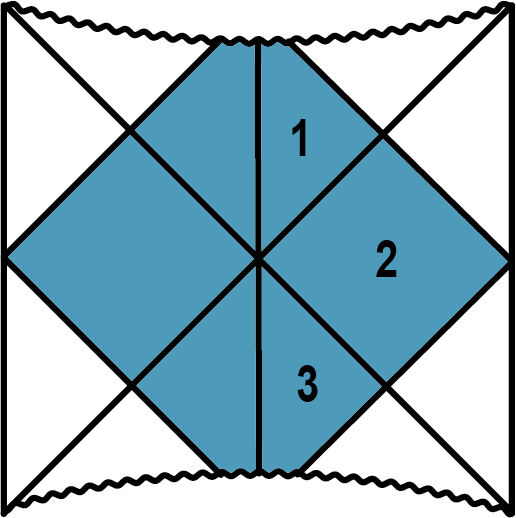
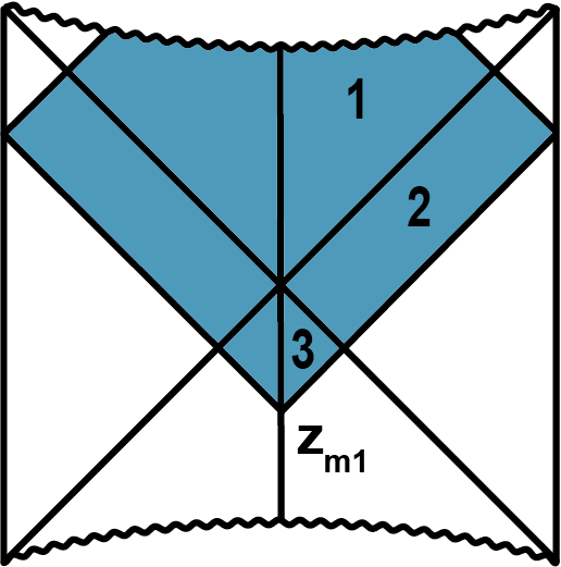
Figure 1: WDW patch for a type $D$ solution. Left: before $t_{c}$. Right: after $t_{c}$.

The eternal black hole solution is symmetric under time reflection $t_{b}\to-t_{b}$, and so it is enough to study the behaviour of complexity for $t_{b}>0$. The time dependence of the WDW patch for type $D$ solutions is shown in figure 1. At $t_{b}=0$, the WDW patch has a hexagonal shape ​​ . As the boundary time increases, at some critical time $t_{b}=t_{c}$ the WDW wedge experiences a discontinuous transition ​​ $\to$ ​​ . For $t<t_{c}$, the complexity rate is identically zero. When the tip of the WDW (a null-like joint) forms at the singularity inside the white hole horizon, there is a peculiar logarithmic divergence in the complexity rate

$$\frac{dI_{\rm WDW}}{dt_{b}}\approx\frac{V_{0}}{16\pi G}A(\infty)\,\log(t_{b}-t_{c})\,,\qquad t_{b}>t_{c}\,,$$ (8)

where $V_{0}$ is the volume of the boundary theory and $A(\infty)>0$ is given by eq. (141). When the limit $t_{b}\to t_{c}$ is approached from $t_{b}>t_{c}$, the complexity rate tends to $-\infty$. This is the same kind of behaviour as in the Schwarzschild case Carmi:2017jqz ; Yang:2017czx .

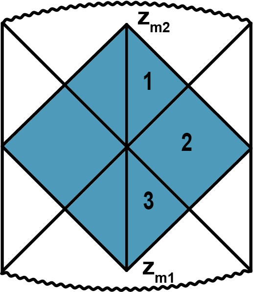
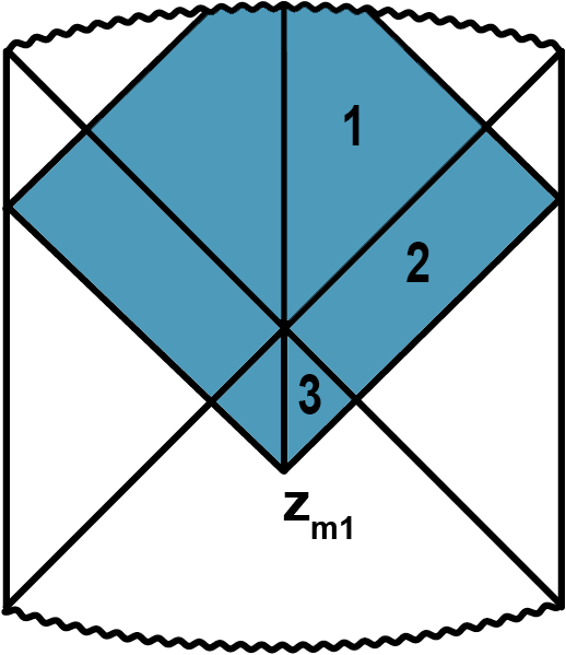
Figure 2: WDW patch for type $U$. Left: before $t_{c}$. Right: after $t_{c}$.

A sketch of the time dependence of the WDW patch for the type $U$ solution is shown in figure 2. In this case, at $t_{b}=0$ the WDW has the shape ​​ . At a critical time $t_{b}=t_{c}$ the shape of the WDW changes abruptly as ​​ $\to$ ​​ . The limit in which the scalar perturbation vanishes outside the Cauchy horizon corresponds to an extreme type $U$ case, in which the singularity approaches the location of the would be Cauchy horizon in the Penrose diagram. In this limit we have that the critical time tends to infinity. Denoting by $\phi_{h}$ the value of the scalar on the event horizon, we find (see appendix H) that the critical time scales as

$$t_{c}=O\left(\frac{1}{\phi_{h}^{2}}\right)\,.$$ (9)

See figure 19 for a plot of the critical time as a function of $\phi_{h}$.

When the tip of the WDW touches the singularity there is a logarithmic divergence in the complexity rate,

$$\frac{dI_{\rm WDW}}{dt_{b}}\approx-\frac{V_{0}}{16\pi G}A(\infty)\,\log(t_{c}-t_{b})\,,\qquad t_{b}<t_{c}\,.$$ (10)

If we approach the limit $t_{b}\to t_{c}$ from $t_{b}<t_{c}$, the complexity rate diverges to $+\infty$. For $t_{b}>t_{c}$ the complexity rate is instead finite. In the $\phi_{h}\to 0$ limit, the value of $A(\infty)$ in eq. (10) can be determined analytically:

• For a neutral scalar $q=0$, the quantity $A(\infty)$ tends to a finite value for $\phi_{h}\to 0$,

  $$A(\infty)\to-\frac{16\pi G}{V_{0}}T_{c}S_{c}\,,$$ (11)

  where $S_{c}$ and $T_{c}$ are the formal entropy and negative temperature computed on the Cauchy horizon, see eq. (134). In this limit the Kasner parameter $\alpha$ diverges.

• For $q\neq 0$, we find that $A(\infty)$ vanishes for $\phi_{h}\to 0$, so that the divergence of the complexity rate at the critical time tends to disappear. In this case the final Kasner parameter $\alpha$ oscillates an infinite number of times as the limit $\phi_{h}\to 0$ is approached.

Thus, there is no direct relation between the divergence in the complexity rate in eq. (10) and the Kasner parameter $\alpha$. Also, the divergence of the complexity rate at critical time in eq. (10) shows that the Lloyd bound can not hold at finite time in this class of models.

We determined analytically the asymptotic action complexity rate in the $\phi_{h}\to 0$ limit. We find that the behavior of the asymptotic action complexity rate is discontinuous for $q\to 0$:

• For the neutral scalar case $q=0$, the asymptotic complexity tends to that of the RN black hole, i.e.

  $$\lim_{t_{b}\to\infty}\frac{dI_{\rm WDW}}{dt_{b}}=T\,S\,-T_{c}\,S_{c}\,,$$ (12)

  where $T$ and $S$ are the temperature and entropy.

• In the charged scalar case $q\neq 0$, we find

  $$\lim_{t_{b}\to\infty}\frac{dI_{\rm WDW}}{dt_{b}}=T\,S\,.$$ (13)

We numerically checked that the Lloyd bound holds for the asymptotic action complexity rate $W_{A}$ in all the parameter space that we investigated.

In geometries with a naked Kasner singularity, the structure of the time dependence of complexity is such that complexity decreases as the singularity is approached Barbon:2015ria ; Bolognesi:2018ion . In that case, however, the singularity is not hidden behind a protective horizon as in the present setup. Eventually, one would expect that there is an intermediate setup for which the complexity ceases to increase for a long time without decreasing, allowing for a parametrically long period of large and constant complexity. This was not achieved in this work. However, we do sustain the believe that such a setup will be eventually found, either semiclassically or perhaps including higher genus effects Iliesiu:2021ari .

We now resume the main new results contained in the paper:

• We numerically compute the Kasner exponent $p_{t}$ as a function of $\phi_{0}$ and $T$ for the charged scalar and we determine if solution is type $U$ or type $D$. See figure 10.

• We investigate the time dependence of volume complexity in a large class of hairy black hole solutions and we provide numerical evidence that the Lloyd bound Lloyd ; Brown:2015lvg is always satisfied in this model.

• We study the time dependence of action complexity in the same class of hairy black hole solutions. The time dependence of action complexity can distinguish between type $D$ and type $U$ solutions. For type $D$ solutions, we find a similar behavior to the Schwarzschild case studied in Carmi:2017jqz . For type $U$ solutions, we find that the complexity rate diverges to $+\infty$ at the critical time $t_{c}$. This is how complexity feels the Kasner singularity.

• The divergence of complexity rate at critical time shows that the Lloyd bound does not hold for action complexity at finite time in this class of solutions. We provide numerical evidence that the Lloyd bounds holds for the asymptotic action complexity rate.

• We find that the Kasner exponents nearby the singularity are not directly correlated with the coefficient of the linear growth at late time $W_{A}$ and with the coefficient of the leading singular behavior of action complexity at the critical time.

Note added: While we were finishing to write this work, Ref. An:2022lvo appeared on the arXiv. There is some overlap with the results presented in this work.

2 The model and the black hole solutions

2.1 Theoretical setting

We consider the Einstein-Maxwell model with a scalar field, with action:

$$S=\frac{1}{16\pi G}\int d^{4}x\sqrt{-g}\left\{R-2\Lambda-\frac{1}{4}F_{\mu\nu}F^{\mu\nu}-g^{\mu\nu}D_{\mu}\phi(D_{\nu}\phi)^{*}-m^{2}\phi\phi^{*}\right\}\,,$$ (14)

where the cosmological constant is

$$\Lambda=-\frac{3}{L^{2}}\,,$$ (15)

and $L$ is the AdS radius. The covariant derivative is

$$D_{\mu}\phi=\partial_{\mu}\phi+iqA_{\mu}\phi\,.$$ (16)

We will consider both the case of neutral scalar field $q=0$ and charged scalar field $q\neq 0$. We will take the scalar mass to be above the Breitenlohner-Freedman (BF) bound Breitenlohner:1982jf

$$m^{2}=-\frac{2}{L^{2}}\,,$$ (17)

and from now on we will set $L=1$ for simplicity.

A generic metric for a planar black hole is

$$ds^{2}=\frac{1}{z^{2}}\left(-fe^{-\chi}dt^{2}+\frac{dz^{2}}{f}+dx^{2}+dy^{2}\right)\,,$$ (18)

where $f$ and $\chi$ are functions of $z$ and the ansatz for the scalar and gauge field is

$$\phi=\phi(z)\,,\qquad A=a(z)dt\,.$$ (19)

The equations of motion are

$$f^{\prime}-\left(\frac{\chi^{\prime}}{2}+\frac{3}{z}\right)f+\frac{3}{z}-\frac{e^{\chi}z^{3}\left(a^{\prime}\right)^{2}}{4}-\frac{m^{2}\phi^{2}}{2z}=0\,,$$

$$\chi^{\prime}-\frac{za^{2}q^{2}\phi^{2}}{f^{2}}e^{\chi}-z(\phi^{\prime})^{2}=0\,,$$

$$a^{\prime\prime}+\frac{\chi^{\prime}}{2}a^{\prime}-\frac{2q^{2}\,\phi^{2}}{fz^{2}}a=0\,,$$

$$\phi^{\prime\prime}-\left(\frac{\chi^{\prime}}{2}+\frac{2}{z}-\frac{f^{\prime}}{f}\right)\phi^{\prime}+\left(\frac{a^{2}q^{2}e^{\chi}}{f^{2}}-\frac{m^{2}}{fz^{2}}\right)\phi=0\,,$$ (20)

with asymptotic conditions at the boundary

$$f|_{z\rightarrow 0}=1\,,\qquad\chi|_{z\rightarrow 0}=0\,,\qquad a|_{z\rightarrow 0}=\mu\,,$$ (21)

where $\mu$ is chemical potential. With our choice of scalar mass, the expansion of the scalar field $\phi$ near the boundary reads

$$\phi=\phi_{0}z+\phi_{1}z^{2}+\dots\,.$$ (22)

With Dirichlet boundary conditions, $\phi_{0}$ can be identified with the source and $\phi_{1}$ with the expectation value of the operator with dimension $\Delta_{+}=2$. On the other hand, with Neumann boundary conditions $\phi_{1}$ is proportional to the source and $\phi_{0}$ to the expectation value of an operator with dimension $\Delta_{-}=1$. We will mainly work with the choice $\Delta_{-}$ that corresponds to Neumann boundary conditions for the scalar field. The empty AdS solution of (20) is

$$f=1\,,\qquad\chi=a=\phi=0\ .$$ (23)

2.2 The Reissner-Nordström black hole

For the Reissner-Nordström (RN) solution we have $\phi,\chi=0$ and

$$f_{\rm RN}(z)=1-\left(\frac{z}{z_{h}}\right)^{3}\left(1+\frac{\rho^{2}z_{h}^{4}}{4}\right)+\frac{\rho^{2}}{4}z^{4}\,,\qquad\rho=\frac{\mu}{z_{h}}\,,$$

$$a(z)=\mu\left(1-\frac{z}{z_{h}}\right)\,,$$ (24)

where $z_{h}$ is the external horizon, $\mu$ is the chemical potential as before, and $\rho$ is the charge density. The RN black hole has a Cauchy horizon at $z=z_{c}$. In terms of $(z_{h},z_{c})$ the solution is:

$$f_{\rm RN}(z)=1-z^{3}\frac{(z_{h}+z_{c})(z_{c}^{2}+z_{h}^{2})}{z_{h}^{3}z_{c}^{3}}+z^{4}\frac{z_{h}^{2}+z_{c}^{2}+z_{h}z_{c}}{z_{h}^{3}z_{c}^{3}}\,,\qquad\rho=\frac{2\sqrt{z_{h}^{2}+z_{c}^{2}+z_{h}z_{c}}}{z_{h}^{\frac{3}{2}}z_{c}^{\frac{3}{2}}}\,,$$ (25)

and has energy density

$$\mathcal{E}=\frac{1}{16\pi G}\frac{2(z_{h}+z_{c})(z_{c}^{2}+z_{h}^{2})}{z_{h}^{3}z_{c}^{3}}\,.$$ (26)

The total black hole charge, mass and entropy are

$$Q=\rho\,V_{0}\,,\qquad M=\mathcal{E}\,V_{0}\,,\qquad S=\frac{V_{0}}{4G}\frac{1}{z_{h}^{2}}\,,$$ (27)

the black hole temperature being in turn

$$T=-\frac{1}{4\pi}f^{\prime}(z_{h})=\frac{(z_{c}-z_{h})(3z_{c}^{2}+2z_{c}z_{h}+z_{h}^{2})}{4\pi z_{c}^{3}z_{h}}\,.$$ (28)

If we send $\rho\rightarrow 0$, we have $z_{c}\to\infty$ and in this limit we recover the Schwarzschild black hole. The extremal limit corresponds to

$$\mu_{e}=\frac{2\sqrt{3}}{z_{h}}\,,$$ (29)

for which $z_{c}=z_{h}$ and the temperature vanishes. It is useful to express $T/\mu$ as a function of $y=z_{c}/z_{h}$, giving

$$\frac{T}{\mu}=\frac{1}{8\pi}\frac{(y-1)(3y^{2}+2y+1)}{y^{3/2}\sqrt{1+y+y^{2}}}\,,$$ (30)

see figure 3 for a plot.

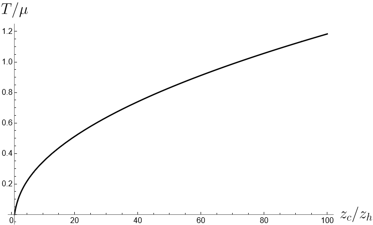
Figure 3: $T/\mu$ as a function of $z_{c}/z_{h}$ for the Reissner-Nordström AdS spacetime.

When we include the scalar backreaction, the inner horizon of the RN black hole, which is unstable, disappears and there is singularity at $z\rightarrow\infty$, just as for the Schwarzchild black hole. This was proved in various theoretical setting in Hartnoll:2020rwq ; Hartnoll:2020fhc ; Cai:2020wrp ; An:2021plu .

2.3 Approximate solution at large $z$: the Kasner limit

The presence of the scalar $\phi$ gives rise to interesting dynamical phenomena, which have been investigated in detail in several theoretical setting in Hartnoll:2020rwq ; Hartnoll:2020fhc ; Frenkel:2020ysx ; Cai:2020wrp ; Henneaux:2022ijt ; Mansoori:2021wxf ; Sword:2021pfm ; Caceres:2022smh . The full system in eq. (20) can in general only be solved numerically. To make the analysis more robust, it is therefore useful to introduce analytical approximations.

In particular, it is convenient to consider a regime in which the scalar $\phi$ scales logarithmically. Numerical analysis confirms that this is a good approximation when $z$ is large enough. Let us assume that we can neglect the electric field $a^{\prime}$, the cosmological constant term, the scalar mass term $m^{2}$ and its charge $q$. The system in eq (20) is then approximately

$$f^{\prime}-\left(\frac{\chi^{\prime}}{2}+\frac{3}{z}\right)f=0\,,\qquad\chi^{\prime}-z(\phi^{\prime})^{2} = 0\,,$$

$$\phi^{\prime\prime}-\frac{\chi^{\prime}\phi^{\prime}}{2}+\left(\frac{f^{\prime}}{f}-\frac{2}{z}\right)\phi^{\prime} = 0\,.$$ (31)

The equations above admit the following exact solution:

$$f=-f_{0}z^{3+\alpha^{2}}\,,\qquad\phi=\alpha\,\sqrt{2}\log z\,,\qquad\chi=2\alpha^{2}\log z+\chi_{0}\,,$$ (32)

where $\alpha$, $f_{0}$, $\chi_{0}$ are integration constants. The behaviour for the metric component $g_{tt}$ is

$$g_{tt}=-f_{0}e^{-\chi_{0}}z^{1-\alpha^{2}}\,.$$ (33)

With the change of variables

$$\tau=\frac{2}{(3+\alpha^{2})\sqrt{f_{0}}}z^{-\frac{3+\alpha^{2}}{2}}\,,$$ (34)

where $\tau\to 0$ corresponds to $z\to\infty$, the metric with $f$ and $\chi$ given by eq. (32) can be put in the Kasner form

$$ds^{2}=-d\tau^{2}+c_{t}\tau^{2p_{t}}dt^{2}+c_{x}\tau^{2p_{x}}(dx^{2}+dy^{2})\,,$$ (35)

where $c_{t},c_{x}$ are constants and the Kasner exponents are

$$p_{t}=\frac{\alpha^{2}-1}{3+\alpha^{2}}\,,\qquad p_{x}=\frac{2}{3+\alpha^{2}}\,.$$ (36)

where $p_{t}$ and $p_{x}$ obey the modified Kasner constraints

$$p_{t}+2p_{x}=1\,,\qquad p_{t}^{2}+2p_{x}^{2}=1-\frac{4\alpha^{2}}{(3+\alpha^{2})^{2}}\,.$$ (37)

The Schwarzchild solution close to the singularity is of Kasner-type, with $\alpha=0$ and $p_{t}=-\frac{1}{3}$. The exponent $p_{x}$ is always positive, and so the transverse direction $x,y$ always experiences a crunch inside the BH in the regime described by eq. (32). The exponent $p_{t}$ is in turn only positive for $\alpha>1$, which gives a contracting ER bridge. It is negative for $\alpha<1$, which corresponds instead to an expanding bridge.

The Kasner approximation in eq. (32) is useful in the regime of large $z$. In particular, for $\alpha>1$ the approximation is stable: if it is satisfied for some $z$, the fields go in a direction such that the approximation becomes even better at larger $z$. In contrast, for $\alpha<1$ the approximation is not stable for a charged black hole. In this case, at large enough $z$ we are forced to consider in eq. (20) the backreaction of the electric field $F_{zt}=a^{\prime}(z)$ on the metric. From the numerical study in Hartnoll:2020fhc we know that, also for $\alpha<1$, there often exists a parametrically large regime in $z$ for which eq. (32) provides a good approximation. However, for $\alpha<1$ we cannot extrapolate the approximation all the way to $z\to\infty$, because at some point the backreaction due to the electric field will be important.

2.4 The Kasner inversion

For $\alpha=\alpha_{0}<1$, if we take into account the backreaction of the electric field the solution in eq. (32) experiences a Kasner inversion, i.e. at some point the exponent $\alpha$ jumps from $\alpha_{0}$ to its inverse $\alpha_{f}=1/\alpha_{0}$,

$$\alpha_{0}\qquad\to\qquad\alpha_{f}=\frac{1}{\alpha_{0}}\,.$$ (38)

For this reason, in the limit $z\to\infty$ we always expect $\alpha>1$. In terms of the Kasner exponent $p_{t}$, the transition is

$$p_{t}\to-\frac{p_{t}}{2p_{t}+1}\,,$$ (39)

and transforms a growing ER bridge ($p_{t}<0$) to a contracting one $(p_{t}>0)$.

This transition could in principle happen both in the case of neutral or charged scalars, because it does not require a direct coupling between the scalar $\phi$ and the gauge field $A_{\mu}$. However, for $q=0$ it seems that this transition is not realised in the parameter space of the model, which was studied in Hartnoll:2020rwq . On the other hand, for a charged scalar this transition is indeed realised in many numerical examples Hartnoll:2020fhc . Due to non-linear effects in the full system of equations of motion (20), multiple Kasner transitions are also possible for $q\neq 0$ when the values of the parametersare fine-tuned .

The Kasner transition in eq. (38) can be derived introducing a more refined approximation to the system in eq. (20), where we keep also the term which is responsible for the backreaction of the Maxwell field strength on the metric, i.e.

$$f^{\prime}-\left(\frac{\chi^{\prime}}{2}+\frac{3}{z}\right)f-\frac{e^{\chi}z^{3}\left(a^{\prime}\right)^{2}}{4\,L^{2}} = 0\,,\qquad\chi^{\prime}-z(\phi^{\prime})^{2}=0\,,$$

$$\phi^{\prime\prime}-\left(\frac{\chi^{\prime}}{2}+\frac{2}{z}-\frac{f^{\prime}}{f}\right)\phi^{\prime} = 0\,.\qquad a^{\prime\prime}+\frac{\chi^{\prime}}{2}a^{\prime}=0\,.$$ (40)

Here we still neglect the cosmological constant term and the effects due to the mass $m$ and the charge $q$ of the scalar field. We can integrate the equation for $a$ as follows

$$a^{\prime}=E_{0}e^{-\frac{\chi}{2}}\,,\qquad a=A_{0}+E_{0}\int e^{-\frac{\chi}{2}}\,dz\,,$$ (41)

where $E_{0}$ and $A_{0}$ are integration constants. With this relation, the equation for $f$ can be put in the form

$$f^{\prime}-f\left(\frac{\chi^{\prime}}{2}+\frac{3}{z}\right)-\frac{E_{0}^{2}z^{3}}{4}=0\,,$$ (42)

and assuming the Kasner behaviour for $f$ and $\chi$ given by eq. (32), then the new term ${E_{0}^{2}z^{3}}/{4}$ dominates the others at large $z$ only for $\alpha<1$.

Equation (42) can be solved as follows

$$\left(\frac{fe^{-\chi/2}}{z^{3}}\right)^{\prime}=\frac{E_{0}^{2}}{4}e^{-\chi/2}\,,\qquad\frac{fe^{-\frac{\chi}{2}}}{z^{3}}=C_{0}+\frac{E_{0}^{2}}{4}\int e^{-\frac{\chi}{2}}\,dz\,,$$ (43)

where $C_{0}$ is an integration constant. We can rewrite the equation involving the second derivative of $\phi$ as

$$\left(\frac{e^{-\frac{\chi}{2}}f\phi^{\prime}}{z^{2}}\right)^{\prime}=0\,.$$ (44)

Combining eqs. (43) and (44) we find

$$\left(\frac{E_{0}^{2}}{4}e^{-\frac{\chi}{2}}\right)z\phi^{\prime}+\left(C_{0}+\frac{E_{0}^{2}}{4}\int e^{-\frac{\chi}{2}}\,dz\,\right)(\phi^{\prime}+z\phi^{\prime\prime})=0\,.$$ (45)

Following Hartnoll:2020fhc , it is convenient to write $\phi$ in terms of an auxiliary function $\psi$ defined by

$$\phi=\sqrt{2}\int\frac{\psi(z)}{z}dz\,.$$ (46)

Note that a constant $\psi(z)=\alpha$ mimics the solution without inversion in eq. (32). The Kasner inversion correponds to a solution which interpolates from an initial $\psi=\alpha_{0}$ to a final $\psi=\alpha_{f}$. Here the physically interesting regime is $0<\alpha_{0}<1$, since otherwise there is no inversion because the backreaction due to the electric field remains small.

In terms of $\psi$, it is possible to show that eq. (45) implies the following differential equation Hartnoll:2020fhc

$$\psi^{\prime\prime}-\frac{2(\psi^{\prime})^{2}}{\psi}+\frac{\psi^{2}\psi^{\prime}}{z}=0\,,$$ (47)

whose solution is

$$\psi\left(\psi-\alpha_{0}\right)^{-\frac{1}{1-\alpha_{0}^{2}}}\left(\frac{1}{\alpha_{0}}-\psi\right)^{-\frac{1}{1-\frac{1}{a_{0}^{2}}}}=\frac{z_{0}}{z}\,,$$ (48)

where $z_{0}$ is an integration constant. In this case $\psi\to\alpha_{0}$ for $z\ll z_{0}$ and $\psi\to\alpha_{f}=1/\alpha_{0}$ for $z\gg z_{0}$. This is indeed the behaviour described in eq. (38).

2.5 Neutral scalar field

Let us now discuss the $q=0$ model, which was studied in detail in Hartnoll:2020rwq . In this case, we can solve explicitly (20) for the gauge field

$$a^{\prime}=-\rho\,e^{-\frac{\chi}{2}}\,,$$ (49)

where $\rho$ is the charge density. Indeed, eq. (49) can be physically derived from the conservation of the electric flux, see appendix A. We end up with a system composed of the remaining differential equations

$$-f^{\prime}+\left(\frac{z\left(\phi^{\prime}\right)^{2}}{2}+\frac{3}{z}\right)f+\frac{\rho^{2}z^{3}}{4}-\frac{\phi^{2}}{z}-\frac{3}{z}=0\,,$$

$$\phi^{\prime\prime}-\frac{z}{2}\left(\phi^{\prime}\right)^{3}+\left(\frac{f^{\prime}}{f}-\frac{2}{z}\right)\phi^{\prime}+\frac{2}{fz^{2}}\phi=0\,,\qquad\chi^{\prime}=z(\phi^{\prime})^{2}\,.$$ (50)

Evaluating the equations above at the horizon $z=z_{h}$, which is defined by the condition $f(z_{h})=0$, we obtain using the expansion $f(z)\approx f^{\prime}(z_{h})(z-z_{h})$,

$$-f^{\prime}(z_{h})+\frac{\rho^{2}z_{h}^{3}}{4}-\frac{\phi^{2}(z_{h})}{z_{h}}-\frac{3}{z_{h}}=0\,,$$

$$\frac{1}{z-z_{h}}\left(\phi^{\prime}(z_{h})+\frac{2}{f^{\prime}(z_{h})z_{h}^{2}}\phi(z_{h})\right)+{\rm finite}=0\,.$$ (51)

In order to get a smooth solution, we must then impose the following condition at the horizon

$$\phi(z_{h})=\phi_{h}\,,\qquad\phi^{\prime}(z_{h})=-\frac{8\phi_{h}}{z_{h}\left(\rho^{2}z_{h}^{4}-4\phi_{h}^{2}-12\right)}\,.$$ (52)

These boundary conditions, together with $f(z_{h})=0$ and the value of $\rho$, are enough to solve the problem. A solution is then determined by the values of $z_{h}$, $\rho$ and $\phi_{h}$.

Alternatively, a given solution can be determined in terms of the temperature $T$ and the sources $\mu$ and $\phi_{0}$ in the dual CFT. The temperature is:

$$T=-\frac{1}{4\pi}f^{\prime}(z_{h})e^{-\frac{\chi(z_{h})}{2}}\,,$$ (53)

and the chemical potential is

$$\mu=a(0)=\rho\int_{0}^{z_{h}}e^{-\frac{\chi}{2}}\,dz\,.$$ (54)

The limit $\phi_{h}\to 0$ can be studied analytically. In this case, the backreaction of the scalar is negligible up to the location of the Cauchy horizon $z=z_{c}$ in the unperturbed RN solution, for which the scalar field $\phi$ identically vanishes. More precisely, the solution is with good approximation the same as the $RN$ for $z<z_{i}$, where

$$z_{i}=z_{c}-\epsilon\,,\qquad\epsilon\to 0\qquad{\rm for}\qquad\phi_{h}\to 0\,.$$ (55)

For $z\approx z_{i}$, the dynamics enters in a highly non-linear regime in which $g_{tt}$ drops exponentially towards zero. This regime was called in Hartnoll:2020rwq the collapse of the Einstein-Rosen (ER) bridge. As can be checked a posteriori, in this limit we can neglect the mass of the scalar field $\phi$. With this approximation, the equations of motion (50) take the following form

$$\left(\frac{e^{-\chi/2}f}{z^{3}}\right)^{\prime}=e^{-\chi/2}\left(\frac{\rho^{2}}{4}-\frac{3}{z^{4}}\right)\,,\qquad\chi^{\prime}=z(\phi^{\prime})^{2}\,,\qquad\left(\frac{e^{-\chi/2}f\phi^{\prime}}{z^{2}}\right)^{\prime}=0\,.$$ (56)

The collapse of the ER bridge happens in a small range of the coordinate $z$, and so it is consistent to set $z\approx z_{i}$ in the equations of motion above, keeping $f$, $\chi$ and $\phi$ as functions of $z-z_{i}$, i.e.

$$\left({e^{-\chi/2}f}\right)^{\prime}=e^{-\chi/2}\left(\frac{\rho^{2}}{4}z_{i}^{3}-\frac{3}{z_{i}}\right)\,,\qquad\chi^{\prime}=z_{i}(\phi^{\prime})^{2}\,,\qquad\left({e^{-\chi/2}f\phi^{\prime}}\right)^{\prime}=0\,.$$ (57)

The equations for the metric functions can be written as

$$\chi^{\prime}f^{2}e^{-\chi}=\tilde{A}\,,\qquad f^{\prime}-\frac{\chi^{\prime}}{2}f=\tilde{B}\,,$$ (58)

where $\tilde{A}$ is an integration constant and

$$\tilde{B}=\frac{\rho^{2}}{4}z_{i}^{3}-\frac{3}{z_{i}}\approx\frac{z_{h}^{2}z_{c}+z_{c}^{3}+z_{h}z_{c}^{2}-3z_{h}^{3}}{z_{h}^{3}z_{c}}>0\,.$$ (59)

Introducing

$$H=z_{i}^{2}g_{tt}=-fe^{-\chi}\,,\qquad G=e^{-\chi}\,,$$ (60)

the solution to (58) takes the form

$$\frac{\tilde{A}}{2\tilde{B}}\log H+H=-\tilde{C}(z-z_{0})\,,\qquad G=\frac{(H^{\prime})^{2}}{\tilde{B}\tilde{C}}\,,$$ (61)

where $z_{0}=z_{c}$ and $\tilde{C}$ are integration constants. In the limit $\phi_{h}\to 0$, we expect that $\tilde{A}\to 0$ while $\tilde{C}\approx f^{\prime}_{RN}(z_{c})=O(\phi_{h}^{0})$. The scalar $\phi$ is given by

$$\phi=-\frac{\tilde{A}^{1/2}}{(\tilde{B}\tilde{C})^{1/2}}\frac{1}{z_{i}^{1/2}}\log(H\tilde{D})\,,$$ (62)

where $\tilde{D}$ is another integration constant. In the limit $\phi_{h}\to 0$, the equation for the scalar is approximately linear for $z<z_{i}$, because the scalar is small. Then the amplitude of the scalar in eq. (62) must scale linearly in $\phi_{h}$, i.e.

$$\tilde{A}^{1/2}=O(\phi_{h})\,,\qquad{\rm for}\qquad\phi_{h}\to 0\,.$$ (63)

For $z\gg z_{0}$ we find that $g_{tt}$ approaches to zero exponentially,

$$g_{tt}=\frac{H}{z_{i}^{2}}\approx\frac{1}{z_{i}^{2}}\exp\left(-\frac{2\tilde{B}\tilde{C}}{\tilde{A}}(z-z_{0})\right)\,,$$ (64)

This approximation can then be matched with the Kasner approximation, which is valid at large $z$. In particular, matching eqs. (32) and (61) we find

$$e^{-\chi_{0}/2}f_{0}=-z^{3}\,e^{-\chi/2}f=z^{3}\frac{H}{G^{1/2}}\approx z_{c}^{3}\frac{\tilde{A}}{2(\tilde{B}\tilde{C})^{1/2}}\,.$$ (65)

From eq. (63) we find that $e^{-\chi_{0}/2}f_{0}=O(\phi_{h}^{2})$ for $\phi_{h}\to 0$.

A numerical approach (see appendix B for our numerical techniques) can be used to solve (50) also away from the limit $\phi_{h}\to 0$. In general, there is a crossover at $z\approx z_{c}$ from a solution qualitatively similar to the RN for $z\ll z_{c}$ and a Kasner regime for $z\gg z_{c}$. In the intermediate region, the metric $g_{tt}$ drops exponentially to a value very close to zero. This drop is very sudden in the $\phi_{h}\to 0$ limit. In all the parameter space investigated in Hartnoll:2020rwq , the solution stabilizes to a Kasner regime with $\alpha>1$ just after the collapse of the ER bridge. For this reason, the Kasner inversion in eq. (38) never takes place. In figure 4 we reproduce the numerical analysis of Hartnoll:2020rwq , showing how the Kasner coefficient $p_{t}$ depends on the parameter space of solutions.

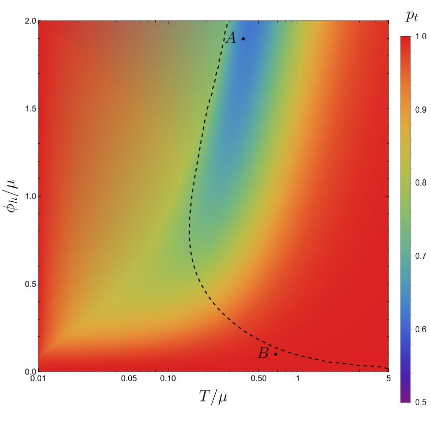
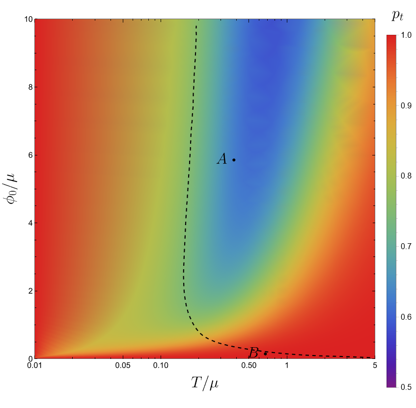
Figure 4: Kasner exponent $p_{t}$ for the neutral scalar case ($q=0$). Left: $p_{t}$ as a function of ${T}/{\mu}$ and ${\phi_{h}}/{\mu}$. Right: $p_{t}$ as a function of ${T}/{\mu}$ and ${\phi_{0}}/{\mu}$. Here we have $p_{t}>0$ and $\alpha>1$ in all the parameter space, and so there is no Kasner inversion. The points marked with letters A and B correspond to the specific examples shown in fig. 5.

For the $q=0$ case it is necessary to introduce a source to get solutions with non-zero scalar profile, i.e. the $\phi_{h}=0$ line corresponds to the $\phi_{0}=0$ line in the two diagrams in figure 4. There is a region at very small temperatures $T/\mu\approx 10^{-4}$ which is not explored in fig. 4. In the extremal RN limit, the near horizon geometry is described by AdS₂ $\times\mathbb{R}^{2}$ with a different AdS radius, and the scalar with mass $m^{2}=-{2}/{L^{2}}$ is below its BF bound, such that condensation can occur Hartnoll:2008kx .

Two examples of numerical solutions are presented in figure 5. In the example (A) we take $\phi_{h}$ rather large and far away from the limit $\phi_{h}\to 0$. Example (B) is closer to the $\phi_{h}\to 0$ limit, and indeed we see that the collapse of the Einstein-Rosen bridge is very fast in the coordinate $z$. Various interesting features can be seen in these plots. It is clear that for all of the solutions the late Kasner behaviour predicted in (32) is present, with $\alpha$ controlling the linear behaviour of $\log f$ and $\phi$ vs. $\log z$. The example (B) is a typical case of small $\phi_{h}$ which is almost identical to RN up to $z=z_{c}$. In the $\phi_{h}\to 0$ limit, the backreaction of the scalar is negligible only up to the “would be” Cauchy horizon $z_{c}$ of the RN solution. At $z_{c}$ there is a transition to the Kasner regime, which is very sharp in the $z$ coordinate. Approaching $\phi_{h}=0$ is not a continuous limit for $z>z_{c}$, since in this limit we have $\alpha\to\infty$ and $p_{t}\to 1$. Then there is a crossover between the RN solution and the Kasner regime discussed in eq. (32). This transition becomes very sharp around $z_{c}$ as $\phi_{h}\to 0$.

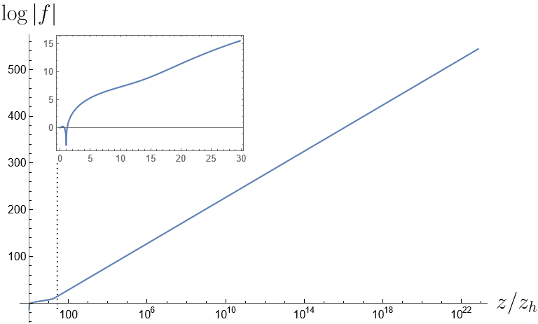
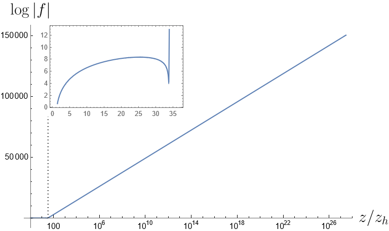
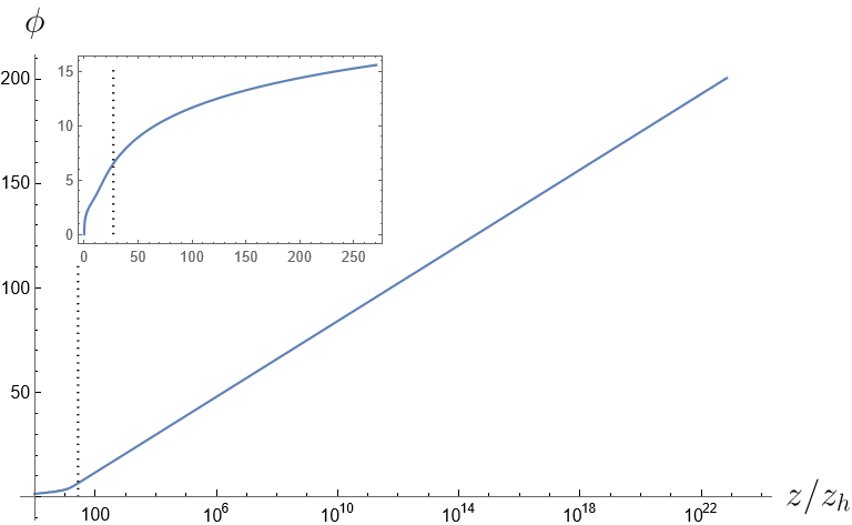
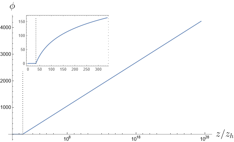
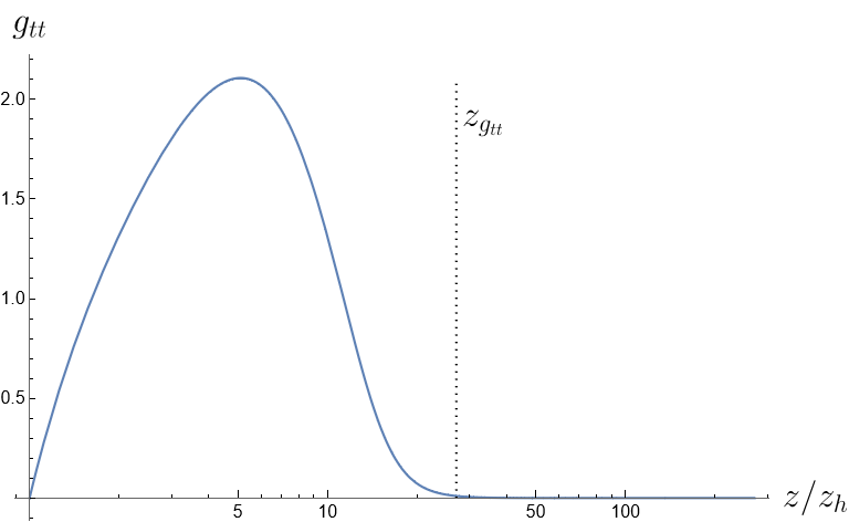
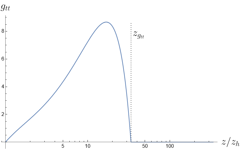
(A)	(B)

Figure 5: Sample solutions for the neutral $q=0$ case. For illustration purposes, we have chosen the values $(z_{h},\rho,\phi_{h})=(1,0.9,1.45)$ for (A) and $(1,0.35,0.035)$ for (B), where the letters match the ones figure 4. The vertical dotted line is the “would be” Cauchy horizon $z_{g_{tt}}$.

In order to describe the causal structure of the solution, it is convenient to use Penrose diagrams. In these diagrams there is always an ambiguity in the choice of the function used in the conformal mapping, so for completeness we explain our conventions in appendix C. There is an important conformally invariant property of the Penrose diagrams which is universal and does not depend on this arbitrary choice Fidkowski:2003nf . Schematically, the Penrose diagram of an eternal asymptotically AdS black hole with a spacelike singularity can be drawn as a square, where the vertical sides are the boundaries of AdS. The spacelike singularity can then bend inwards or outwards the horizontal sides of the square inside the black hole horizon. The direction of this bending is a conformally invariant property, which can be established as follows: let us prepare a couple of ingoing radial lightlike geodesics from the left and the right boundaries at time $t_{b}=0$, and ask whether they meet before reaching the singularity or not. If the singularity coincides with the horizontal line of the square, the two light rays meet exactly at the singularity. If instead the singularity is bending upwards the top side of the square, the two rays meet before intersecting the singularity; finally, if the singularity is bending the top side of the square downwards, the two light rays never meet. This shows that the bending of the singularity is a physical property and does not depend on the choice of conventions used to construct the Penrose diagram.

For the non-rotating BTZ black hole in AdS₃ Banados:1992wn , the singularity lies exactly on the horizontal line. For Schwarzschild AdS_d black holes with $d>3$ the singularity bends the top side downwards. In the case of the black holes discussed in this section, we can in general achieve in the parameter space both upwards and downwards bending of the top side of the Penrose diagram. The kind of bending of the singularity in the Penrose diagram, as we will find in section 4, will influence the time dependence of the action complexity. For convenience, we will denote a solution with the singularity with upper bending as type $U$ and one with the singularity with lower bending as type $D$.

The black dashed line in figure 4 separates two shapes of Penrose diagram: the solutions on the left side of the line are of type $U$, while the ones on the right side are of type $D$. In particular, in the $\phi_{h}\to 0$ limit, the singularity approaches the Cauchy horizon of the RN black hole, and so the bending is up. In figure 6 we show two examples of these Penrose diagram; we plot on the diagram the value of $e^{-\chi}$, which gives a measure of how much the solution is different from the RN limit, which has $\chi=0$.

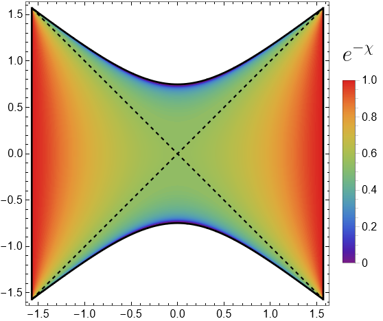
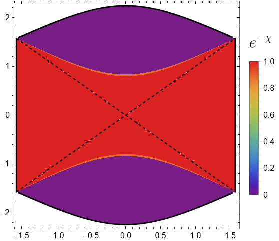
(A)	(B)

Figure 6: Penrose diagrams for the sample solutions A and B, marked in fig. 4 and whose field profiles are shown in fig. 5. On the right, we see that for case B, which is close to the limit $\phi_{h}\to 0$, the collapse of the ER bridge is very fast, as mentioned in the main text. We refer to appendix C for the definition of the coordinates of the Penrose diagram.

2.6 Charged scalar field

The explicit examples studied in Hartnoll:2020fhc correspond to the zero source limit, which is known as for holographic superconductors Hartnoll:2008vx ; Hartnoll:2008kx . In the charged case, the main term which can induce condensation of the scalar close to the horizon is the term in the Lagrangian coming from scalar covariant derivative,

$$-q^{2}g^{tt}(A_{t})^{2}\phi\phi^{*}\,.$$ (66)

This term induces a tachyonic mass term for the scalar in the region laying just outside the horizon, where $g^{tt}\to-\infty$ and $A_{t}\to 0$. This is the reason for the condensation of the scalar in the bulk to be rather common in the charged case, even with a vanishing boundary source. Two well studied boundary conditions for holographic superconductors are

• Dirichlet, which is realised for $\phi_{0}=0$ in eq. (22), with expectation value $\phi_{1}$.

• Neumann, which is realised by $\phi_{1}=0$ in eq. (22), with expectation value $\phi_{0}$.

For both boundary conditions above, at fixed $\rho$ there is a critical temperature $T_{c}$ such that the expectation values are non-zero for $T<T_{c}$. By dimensional analysis, the critical temperature must be proportional to $\sqrt{\rho}$, i.e.

$$T_{c}=C(q)\,{\rho}^{1/2}\,,$$ (67)

where $C(q)$ is a function of the charge. For a plot of $C(q)$ for Neumann and Dirichlet boundary conditions, see fig. 2 of Hartnoll:2008kx . In the regime of large $q$, we have

$$C(q) \approx 0.12\,\sqrt{q}\qquad{\rm for\,Dirichlet}\,,$$

$$C(q) \approx 0.23\,\sqrt{q}\qquad{\rm for\,Neumann}\,.$$ (68)

Just below the critical temperature $T_{c}$ the condensate is negligible on the solution, at least outside the Cauchy horizon. Then, very close to $T_{c}$ the solution is given in good approximation by the RN solution. Using expressions (28) and (25) to express $(T,\rho)$ in terms of $(z_{c},z_{h})$, we find that the critical temperature $T_{c}$ corresponds to the value of $y=z_{c}/z_{h}$ obtained by solving the following equation

$$\frac{3y^{3}-y^{2}-y-1}{4\sqrt{2}\pi\sqrt[4]{y^{9}\left(y^{2}+y+1\right)}}=C(q)\,.$$ (69)

This expression, in combination with the plot of $C(q)$ in Hartnoll:2008kx , can be use to find the holographic superconductor regime in the parameter space.

As for the uncharged case, the $\phi_{h}\to 0$ limit can also be studied analytically when $q\neq 0$. Once more, in this limit the backreaction of the scalar is negligible up to $z=z_{i}$, see eq. (55). For $z\approx z_{i}$, we have again the collapse of the Einstein-Rosen bridge. As can be checked a posteriori, to study the collapse of the bridge we can neglect the mass of the scalar field $\phi$ and the electric source term in Maxwell’s equation. In particular, the gauge field $a$ still satisfies with good approximation eq. (49). The equations of motion (20) then take the form

$$\left(\frac{e^{-\chi/2}f}{z^{3}}\right)^{\prime}={e^{-\chi/2}}\left(\frac{\rho^{2}}{4}-\frac{3}{z^{4}}\right)\,,\qquad\chi^{\prime}=\frac{za^{2}q^{2}\phi^{2}}{f^{2}}e^{\chi}+z(\phi^{\prime})^{2}\,,$$

$$\left(\frac{e^{-\chi/2}f\phi^{\prime}}{z^{2}}\right)^{\prime}=-\frac{1}{z^{2}}\frac{a^{2}q^{2}e^{\chi/2}}{f}\phi\,.$$ (70)

The collapse takes place in a small range of the coordinate $z$, so that as in the uncharged case it is consistent to set $z\approx z_{i}$ in the equations of motion above. In correspondence with the collapse, the field $\chi$ rapidly becomes large so that from eq. (49) the gauge field $a$ can be taken to be practically constant, i.e. $a(z)=a_{0}$. With these simplifications, we must solve the system

$$\left({e^{-\chi/2}f}\right)^{\prime}={e^{-\chi/2}}\left(\frac{\rho^{2}}{4}z_{i}^{3}-\frac{3}{z_{i}}\right)\,,\qquad\chi^{\prime}=z_{i}\left(\frac{a_{0}^{2}q^{2}\phi^{2}}{f^{2}}e^{\chi}+(\phi^{\prime})^{2}\right)\,,$$

$$\left({e^{-\chi/2}f\phi^{\prime}}\right)^{\prime}=-\frac{a_{0}^{2}q^{2}e^{\chi/2}}{f}\phi\,.$$ (71)

It turns out that the solution for $f$ and $\chi$ has the same functional form as for $q=0$. The functional form of the scalar field $\phi$ is now different, however. We can solve for $\phi$ in terms of $\chi$ and $f$,

$$\phi(z)=\Phi_{0}\,\cos\left(q\,a_{0}\,\int_{z_{i}}^{z}\frac{e^{\chi/2}}{f}dz+\varphi_{0}\right)\,,$$ (72)

where $\Phi_{0}$ and $\varphi_{0}$ are integration constants. Using the relation

$$q^{2}\phi^{2}a_{0}^{2}+e^{-\chi}f^{2}(\phi^{\prime})^{2}=q^{2}\Phi_{0}^{2}a_{0}^{2}\,,$$ (73)

we get the same system as for $q=0$, see eq. (58), with $\tilde{B}$ given by eq. (59) and

$$\tilde{A}=z_{i}q^{2}\Phi_{0}^{2}a_{0}^{2}\,.$$ (74)

The solution is given by eq. (61), with eq. (65) still holding. Note that in the $\phi_{h}\to 0$ limit we still have $e^{-\chi_{0}/2}f_{0}=O(\phi_{h}^{2})$, because $\Phi_{0}=O(\phi_{h})$.

The system can be solved numerically also away from the limit $\phi_{h}\to 0$, as done in Hartnoll:2020fhc . See appendix B for a description of our numerical methods.

In particular, if we consider the limit $\phi_{h}\to 0$ keeping $T$ and $\rho$ fixed, we find that after the collapse of the ER bridge the solution flows to a Kasner regime, with parameter $\alpha(\phi_{h})$. As a function of $\phi_{h}$, the Kasner parameter $\alpha(\phi_{h})$ is not continuous for $\phi_{h}\to 0$, and it oscillates between values of $\alpha$ which can be bigger or lower than one. In particular, if the value of $\alpha$ after the collapse is less than one we see that there is a Kasner inversion, which in the approximation discussed in 2.4 brings $\alpha\to 1/\alpha$. Something special happens in the limit $\alpha\to 0$: in this case the approximations used in section 2.4 fail, because we should also take into account terms involving the charge of the scalar field. In this case multiple Kasner inversions are possible, see Henneaux:2022ijt for a recent study with the billiard approach.

In figure 7 we show an example of a solution without inversions, while in figure 8 we show an example with one inversion. Penrose diagrams for these solutions are shown in figure 9.

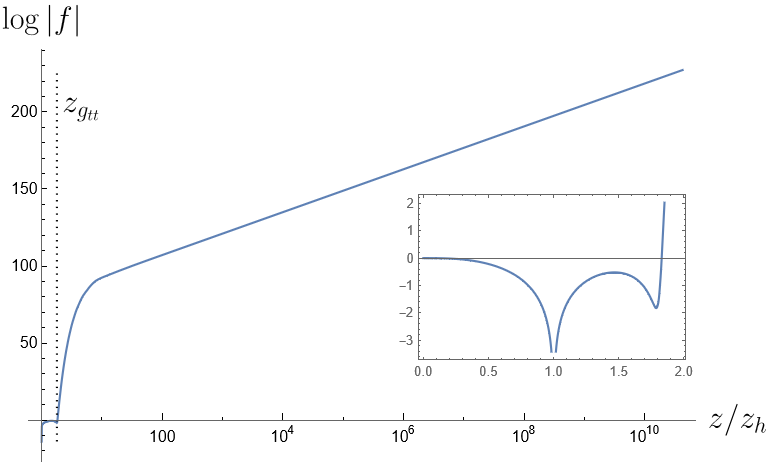
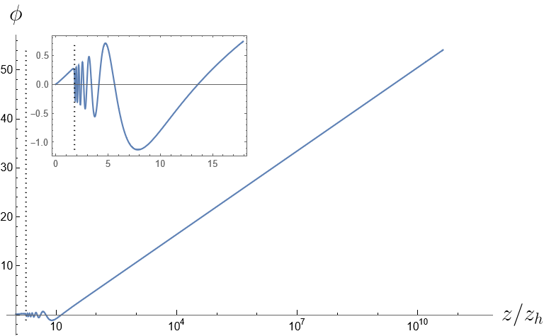
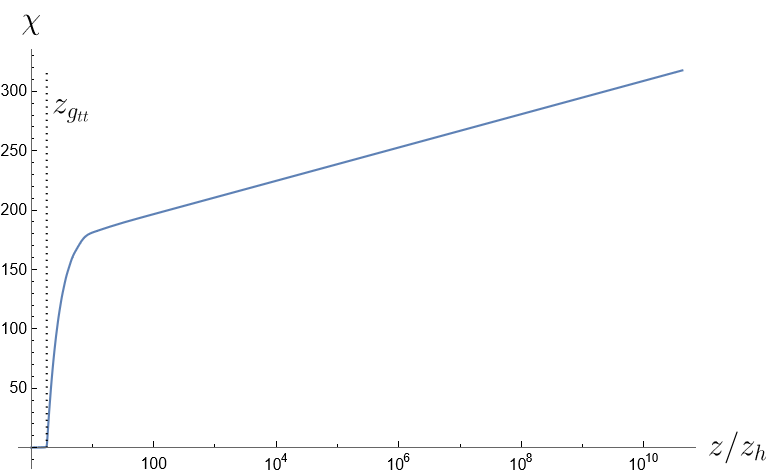
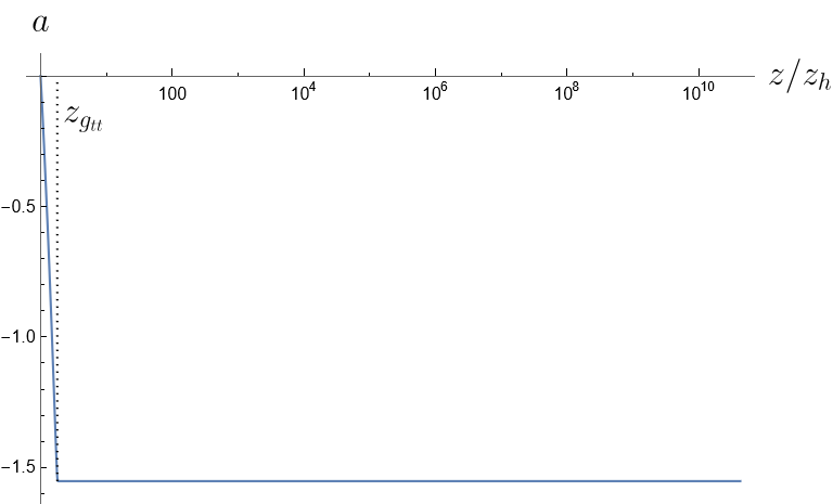
Figure 7: Sample solution for the charged case, without Kasner inversion. For illustration purposes, we have chosen the values $\rho=2,\phi_{h}=0.16,z_{h}=1,q=1$ and $\chi_{h}=0.1$. The vertical dotted line is the “would be” Cauchy horizon $z_{g_{tt}}$. In the little boxes we display a magnification of the plots near $z_{h}=1$.

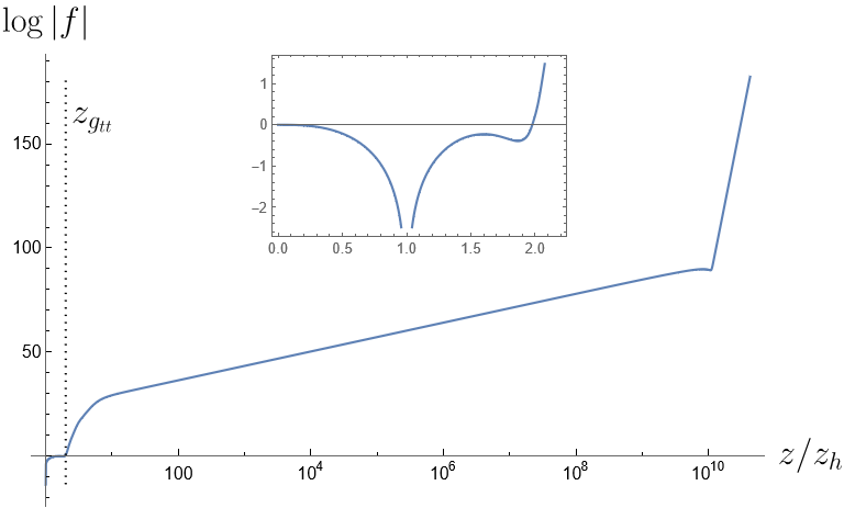
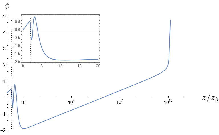
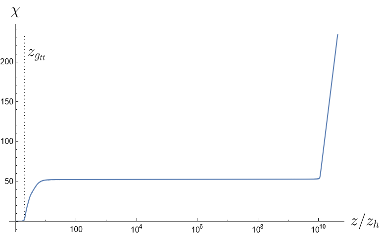
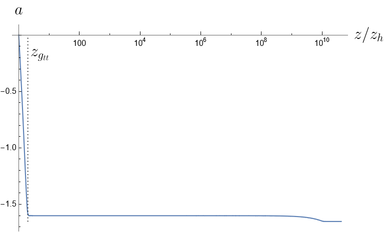
Figure 8: Sample solution for the charged case, with a single Kasner inversion. For illustration purposes, we have chosen the values $\rho=2,\phi_{h}=0.3,z_{h}=1,q=1$ and $\chi_{h}=0.1$. The vertical dotted line is the “would be” Cauchy horizon $z_{g_{tt}}$.

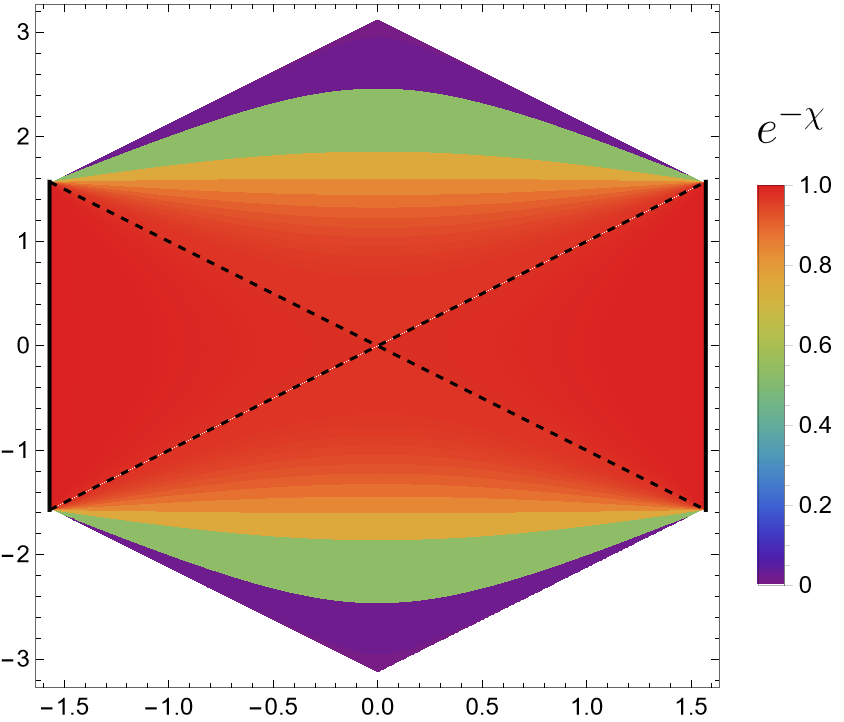
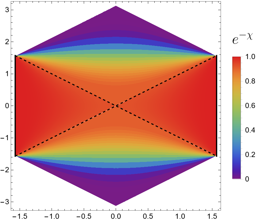
Figure 9: Penrose diagrams for the charged solutions shown in Figures 7 left, and 8 right.

Figure 10 displays a sketch of the Kasner exponent as a function of $\phi_{0}/\mu$ and $T/\mu$. Something similar could be obtained using $\sqrt{q\phi_{1}}/\mu$ instead, however the value of this condensate is very large for $q=1$ as previously found in Hartnoll:2008kx , meaning the plot becomes less clear to visualize. For this reason we choose not to display it here.

Figure 10: The Kasner exponent $p_{t}$ as a function of the parameter space for $q=1$. The black solid line is the line of zero source $\phi_{1}=0$ with spontaneous condensation. The white region in this plot is where our numeric procedure didn’t converge. The plot shows the last value of $p_{t}$ displayed by our solutions at the maximum possible value of $z$. The dashed line divides Type U (below) and type D (above) solutions.

2.7 A conserved quantity

Inserting the ansatz (18,19) into the action (14) we obtain

$$S = \frac{V_{0}}{16\pi G}\int dz\left\{-\frac{e^{-\frac{\chi}{2}}f\chi^{\prime}}{z^{3}}-\frac{12fe^{-\frac{\chi}{2}}}{z^{4}}+\frac{4f^{\prime}e^{-\frac{\chi}{2}}}{z^{3}}+\left(\frac{e^{-\frac{\chi}{2}}f\chi^{\prime}}{z^{2}}-\frac{e^{-\frac{\chi}{2}}f^{\prime}}{z^{2}}\right)^{\prime}\right.$$

$$\qquad\qquad\quad\left.+\frac{6e^{-\frac{\chi}{2}}}{z^{4}}+\frac{e^{\frac{\chi}{2}}(a^{\prime})^{2}}{2}-\frac{e^{-\frac{\chi}{2}}f|\phi^{\prime}|^{2}}{z^{2}}+\frac{e^{-\frac{\chi}{2}}}{z^{4}}\left(\frac{z^{2}e^{\chi}q^{2}a^{2}}{f}-m^{2}\right)|\phi|^{2}\right\}.$$

This action is invariant under the symmetry Gubser:2009cg

$$z\to\lambda z\,,\qquad\chi\to\chi-6\log\lambda\,,\qquad a\to\lambda^{2}a\,,$$ (76)

with fixed $f$ and $\chi$. From this invariance, it follows that the quantity

$$\tilde{Q}=e^{\frac{\chi}{2}}\left(\frac{(fe^{-\chi})^{\prime}}{z^{2}}-aa^{\prime}\right)\,,$$ (77)

is conserved, i.e. $\tilde{Q}^{\prime}=0$, as can be checked from the equations of motion (20). For the RN solution, the conserved quantity in eq. (77) is

$$\tilde{Q}=\frac{z_{h}\rho^{2}}{4}-\frac{3}{z_{h}^{3}}\,.$$ (78)

In this case $\tilde{Q}$ is generically negative and vanishes in the extremal limit.

In order to compute $\tilde{Q}$ in the Kasner regime eq. (32), let us first discuss the screening of electric charge. We can write in general $a^{\prime}$ as

$$a^{\prime}=-\tilde{\rho}(z)\,e^{-\frac{\chi}{2}}\,,$$ (79)

in such a way that $\tilde{\rho}(0)=\rho$. We can introduce $\rho_{f}=\tilde{\rho}(\infty)$. Using the equations of motion, we find:

$$\tilde{\rho}^{\prime}(z)=-2L^{2}q^{2}\,a\,\frac{\phi^{2}e^{\frac{\chi}{2}}}{fz^{2}}\,,\qquad\tilde{\rho}(z)=\rho-2L^{2}q^{2}\,\int_{0}^{z}a\,\frac{\phi^{2}e^{\frac{\chi}{2}}}{f\tilde{z}^{2}}\,d\tilde{z}\,.$$ (80)

If we insert the approximation in eq. (32) in the conserved quantity in eq. (77), we get

$$\tilde{Q}=f_{0}e^{-\frac{\chi_{0}}{2}}(\alpha^{2}-3)+\tilde{\rho}(z)a(z)\,.$$ (81)

We will see that this relation plays an important role in determining the asymptotic complexity rate for the action conjecture.

In particular, it is interesting to consider the $\phi_{h}\to 0$ limit. In this case, for $z<z_{i}$ defined in eq. (55), the profiles $f$, $\chi$ and $a$ are given by the RN solution. We can then compare the conserved charge $\tilde{Q}$ of the RN solution in eq. (78) with the one of the final Kasner in eq. (81), i.e.

$$\tilde{Q}=\frac{z_{h}\rho^{2}}{4}-\frac{3}{z_{h}^{3}}=f_{0}e^{-\frac{\chi_{0}}{2}}(\alpha^{2}-3)+\rho_{f}\,a(\infty)\,.$$ (82)

In the limit $\phi_{h}\to 0$, from the analytic solutions in eq. (61), we have that $\chi$ becomes suddenly very large at the would be Cauchy horizon $z_{c}$. Moreover, from the equations of motion eq. (20) we know that $\chi$ is a monotonic function of $z$. Then, from eq. (79), we have that $a$ approaches a constant for $z>z_{c}$. Then it follows that

$$a(\infty)\approx a_{\rm RN}(z_{c})=-(z_{c}-z_{h})\rho\,.$$ (83)

Let us now distinguish the two cases:

• For $q=0$, there is no screening of electric charge, i.e. $\tilde{\rho}(z)=\rho=\rho_{f}$. Using this result in eq. (82), we find a useful relation between $\alpha$, $f_{0}$ and $\chi_{0}$ valid in the $\phi_{h}\to 0$ limit:

  $$f_{0}e^{-\frac{\chi_{0}}{2}}(\alpha^{2}-3)=\frac{(z_{c}-z_{h})(z_{c}^{2}+2z_{h}z_{c}+3z_{h}^{2})}{z_{h}^{3}z_{c}^{3}}\,.$$ (84)

  From eq. (65) we find

  $$f_{0}e^{-\frac{\chi_{0}}{2}}=O(\phi_{h}^{2})\,.$$ (85)

  As a consequence, $\alpha=O(1/\phi_{h})$, as can be checked from numerical calculations. We can approximate the previous relation for $\phi_{h}\to 0$ as follows

  $$\alpha^{2}=\frac{1}{f_{0}e^{-\frac{\chi_{0}}{2}}}\frac{(z_{c}-z_{h})(z_{c}^{2}+2z_{h}z_{c}+3z_{h}^{2})}{z_{h}^{3}z_{c}^{3}}\,.$$ (86)

• For the first Kasner region we have that eq. (85) still holds because the solution in eq. (61) and the estimate eq. (65) still hold also for $q\neq 0$. During a Kasner inversion, we expect that the value of $f_{0}e^{-\frac{\chi_{0}}{2}}$ stays almost constant, because from equations of motion we have

  $$\left(\frac{e^{-\chi/2}f}{z^{3}}\right)^{\prime}={e^{-\chi/2}}\left(\frac{\tilde{\rho}^{2}}{4}-\frac{3}{z^{4}}\right)\,,$$ (87)

  and, also, we have that $\chi$ is large in the $\phi_{h}\to 0$ limit. The exponent $\alpha$ does not tend to infinity; instead, the value of $\alpha$ after the final inversion oscillates wildly for $\phi_{h}\to 0$ among all possible values from $1$ to $\infty$. As a consequence of eq. (82) we have

  $$\frac{\rho_{f}}{\rho}=\frac{1+2y+3y^{2}}{4(1+y+y^{2})}\,,\qquad y=\frac{z_{c}}{z_{h}}\,.$$ (88)

3 Volume complexity

In this section we will first treat with a unified approach different extremal surfaces with different dimensions $k$, and then we will focus on the $k=3$ case, which is the one relevant for the volume conjecture. Our results are consistent with Yang:2019gce , which focuses on the charged scalar case with vanishing external sources.

3.1 Extremal bulk surfaces

It is interesting to probe the asymptotically AdS₄ black hole geometry with extremal bulk surfaces with different dimensions. In particular, the length of dimension one spacelike curves is related to correlators of heavy scalar operators in the WKB approximation Balasubramanian:1999zv ; Fidkowski:2003nf ; Kraus:2002iv ; Festuccia:2005pi ; Festuccia:2008zx . The area of dimension two extremal surfaces is the holographic dual of the entanglement entropy Ryu:2006bv ; Hubeny:2007xt ; Hartman:2013qma . In the CV conjecture, the complexity is dual to the volume of dimension three extremal bulk surfaces Susskind:2014rva ; Stanford:2014jda ; Carmi:2017jqz . In this section we will briefly discuss how to evaluate these three functionals in the black hole solution that we discussed in section 2.

It is useful to change variables, introducing the lightcone coordinate $v$ defined by

$$dv=dt-\frac{e^{\frac{\chi}{2}}}{f}dz\,,$$ (89)

where $v={\rm constant}$ correspond to the ingoing radial null geodesics. The metric (18) in the coordinates $(v,z,x,y)$ reads

$$ds^{2}=\frac{1}{z^{2}}\left(-fe^{-\chi}dv^{2}-2e^{-\frac{\chi}{2}}dvdz+dx^{2}+dy^{2}\right)\,.$$ (90)

Let us then consider the following particular cases of extremal surfaces with different dimensions:

• A spacelike radial geodesic (with constant $x$ and $y$), parametrized by $z=z(\lambda)$ and $v=v(\lambda)$. The length is

  $$\ell=\int d\lambda\,\frac{1}{z}\sqrt{-2\dot{v}\dot{z}e^{-\frac{\chi}{2}}-fe^{-\chi}\dot{v}^{2}}\,.$$ (91)

• A dimension two surface with constant $y$, parametrized by $(\lambda,x)$. The area functional is

  $$A=L_{x}\int d\lambda\,\frac{1}{z^{2}}\sqrt{-2\dot{v}\dot{z}e^{-\frac{\chi}{2}}-fe^{-\chi}\dot{v}^{2}}\,.$$ (92)

  where $L_{x}=\int dx$ is a cutoff length in the $x$ direction.

• A dimension three surface, parametrized by $(\lambda,x,y)$. The volume functional is

  $$V=V_{0}\int d\lambda\,\frac{1}{z^{3}}\sqrt{-2\dot{v}\dot{z}e^{-\frac{\chi}{2}}-fe^{-\chi}\dot{v}^{2}}\,.$$ (93)

  where $V_{0}=\int dxdy$ is a cutoff area in the $x,y$ plane.

3.2 Equations of motion

We can treat the three functionals as particular cases of the same functional

$$S_{k}=\int d\lambda\,\frac{1}{z^{k}}\sqrt{-2\dot{v}\dot{z}e^{-\frac{\chi}{2}}-fe^{-\chi}\dot{v}^{2}}=\int d\lambda\,\mathcal{L}_{k}\,.$$ (94)

Since $S_{k}$ is translationally invariant in $v$, we can obtain the conserved quantity

$$E_{k}=-\frac{\partial\mathcal{L}_{k}}{\partial\dot{v}}=\frac{1}{z^{k}}\frac{\dot{z}\,e^{-\frac{\chi}{2}}+\dot{v}fe^{-\chi}}{\sqrt{-2\dot{v}\dot{z}e^{-\frac{\chi}{2}}-fe^{-\chi}\dot{v}^{2}}}\,.$$ (95)

Following Belin:2021bga , it is convenient to choose the parameter $\lambda$ in this way

$${z^{k}}\sqrt{-2\dot{v}\dot{z}e^{-\frac{\chi}{2}}-fe^{-\chi}\dot{v}^{2}}=e^{-\frac{\chi}{2}}\,.$$ (96)

With this choice, from eq. (95) we obtain

$$\dot{v}=(E_{k}-\dot{z})\frac{e^{\frac{\chi}{2}}}{f}\,,$$ (97)

which, inserted in eq. (96) gives

$$\dot{z}^{2}+V_{k}(z)=E_{k}^{2}\,,\qquad V_{k}(z)=-\frac{e^{-\chi}\,f}{z^{2k}}\,.$$ (98)

The problem is recasted as the motion of a classical non-relativistic particle in a potential $V_{k}(z)$.

3.3 The time dependence

Using eqs. (96, 98), the functional $S_{k}$ in eq. (94) can be written as follows

$$S_{k}=\int_{z_{\epsilon}}^{z_{t}}\frac{dz}{z^{k}\sqrt{f+E_{k}^{2}z^{2k}e^{\chi}}}\,.$$ (99)

$z_{\epsilon}$ is the UV cutoff and $z_{t}$ is the turning point. The value of $z_{t}$ can be obtained setting $\dot{z}=0$ in eq. (98):

$$V_{k}(z_{t})=E_{k}^{2}\,.$$ (100)

The turning point $z_{t}$ requires $f(z_{t})\leq 0$, and so it is inside the horizon $z_{h}$. The quantity $E_{k}$ is function of the boundary time $t_{b}$ at which the probe is anchored. Note also that for $z_{t}=z_{h}$, we have that $E_{k}=0$. As a convention, we set $t_{b}=0$ for $E_{k}=0$.

The difference in $v$ coordinates

$$v\left(z_{t}\right)-v\left(z_{\epsilon}\right)=\int_{z_{\epsilon}}^{z_{t}}\frac{dz}{f}\left(\frac{e^{\chi}z^{k}E_{k}}{\sqrt{f+e^{\chi}E_{k}^{2}z^{2k}}}-e^{\frac{\chi}{2}}\right)\,.$$ (101)

The boundary time can be obtained by integrating eq. (89)

$$\int_{z_{\epsilon}}^{z_{t}}dt=\int_{z_{\epsilon}}^{z_{t}}dv+\int_{z_{\epsilon}}^{z_{t}}\frac{dz}{f}e^{\frac{\chi}{2}}\,.$$ (102)

which gives

$$t(z_{t})-t(z_{\epsilon})=v(z_{t})-v(z_{\epsilon})+\int_{z_{\epsilon}}^{z_{t}}\frac{dz}{f}e^{\frac{\chi}{2}}\,,$$ (103)

By symmetry argument at the turning point $t(z_{t})=0$. We can then solve for the boundary time:

$$t_{b}=t(z_{\epsilon})=-\int_{z_{\epsilon}}^{z_{t}}\frac{dz}{f}\frac{e^{\chi}z^{k}E_{k}}{\sqrt{f+e^{\chi}E_{k}^{2}z^{2k}}}\,.$$ (104)

Using eq. (104), we can rewrite $S_{k}$ in eq. (99) as follows

$$S_{k}=\int_{z_{\epsilon}}^{z_{t}}\frac{\sqrt{f+E_{k}^{2}z^{2k}e^{\chi}}}{z^{k}f}dz+E_{k}t_{b}$$ (105)

Taking time derivative of (105) and using eq. (100), we find

$$\frac{dS_{k}}{dt_{b}}=E_{k}\,.$$ (106)

This proves that the derivative of $S_{k}$ with respect $t_{b}$ is exactly $E_{k}$. Using the potential $V_{k}$ is defined in eq. (98), we can express the time derivative of $S_{k}$ as a function of $z_{t}$ as follows:

$$\frac{dS_{k}}{dt_{b}}=\sqrt{V_{k}(z_{t})}\,.$$ (107)

The relation between boundary time $t_{b}$ and $z_{t}$ must be determined numerically, by integrating eq. (104).

We can write eq. (104) in the following form

$$t_{b}=\int_{z_{\epsilon}}^{z_{t}}\,\frac{1}{(-fe^{-\chi/2})}\frac{1}{\sqrt{E_{k}^{2}-V_{k}(z)}}\,dz\,.$$ (108)

Figure 11 shows a plot of $\sqrt{V_{3}}$ as a function of $t_{b}$.

Figure 11: Volume complexity rate as a function of time for a black hole with $\rho=2$, $z_{h}=1$ and $q=1$.

Note that the integrand in eq. (108) is diverging for $z=z_{t}$, since $E_{k}^{2}=V_{k}(z_{t})$. In order for the result of the integral to diverge logarithmically, we have to impose that $E_{k}^{2}-V_{k}(z)$ is quadratic in $z$ for $z=z_{t}$. For this reason, the late time limit $t_{b}\to\infty$ corresponds to a maximum of $V_{k}(z_{t})$.

For the Schwarzschild case, $V_{2,3}$ have always a unique extremal point, which is a maximum. On the other hand $V_{1}$ is a monotonic function which has no extremal points. For this reason, spacelike geodesic can pass arbitrarily near the singularity Fidkowski:2003nf . Instead dimension two and three extremal surfaces are respectively stuck at the value of $z$ corresponding to the maximum of $V_{2}$ and $V_{3}$.

In the RN case, we have that $V_{k}$ has always a unique extremal point, which is a maximum, at a finite value of $z<z_{c}$. So, no extremal surface can approach the singularity.

If we consider the model in eq. (14), we have that, in the $\phi_{h}\to 0$ limit, the field profiles tend to the RN solution for $z<z_{c}$. So, in this limit, the potential is the same as in the RN case and it has a maximum for $z_{h}<z<z_{c}$. The potential may have additional extremal points for $z>z_{c}$. Using the Kasner approximation in eq. (32), we get that at large $z$

$$V_{k}(z)=f_{0}e^{-\chi_{0}}z^{3-2k-\alpha^{2}}\,.$$ (109)

For $k>1$, we get that $V_{k}(z)$ has no maximum in the Kasner region. As pointed out in Hartnoll:2020fhc , for geodesics ($k=1$) we can get another maximum of $V_{k}(z)$ in correspondence of the Kasner inversion. In this case there exist values of the boundary time for which multiple extremal surfaces are possible. It would be interesting to understand the physical meaning of these multiple solutions.

3.4 Asymptotic complexity rate

The asymptotic volume complexity rate is given by

$$W_{V}=\lim_{t_{b}\to\infty}\frac{d\,C_{V}}{d\,t_{b}}=\frac{V_{0}}{G}\sqrt{V_{3}(z_{\rm max})}\,,$$ (110)

where $z_{\rm max}$ is the position of the maximum of $V_{3}(z)$, see eq. (98). For the Schwarzchild solution we have

$$W_{V}=\frac{V_{0}}{2G}\frac{1}{z_{h}^{3}}=\frac{8\pi}{3}\,TS\,.$$ (111)

In the extremal limit, for the RN solution the rate vanishes and at the first order in $z_{c}-z_{h}$ is

$$W_{V}\approx\sqrt{\frac{3}{2}}\,\frac{V_{0}}{G}\frac{z_{c}-z_{h}}{z_{h}^{4}}=\sqrt{\frac{3}{2}}\,\frac{8\pi}{3}\,TS\,.$$ (112)

We expect that the asymptotic complexity rate, in units of $TS$, is a slowly varying function of the parameters of the model. This is consistent with the numerical results shown in figure 12. In figure 13 we show the behavior at constant temperature of the asymptotic volume complexity, as a function of $\phi_{0}/\mu$.

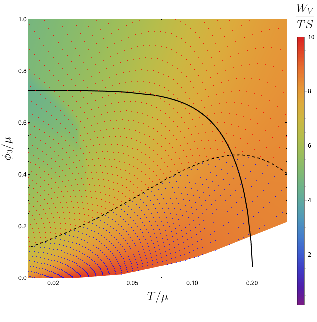
Figure 12: Asymptotic volume complexity rate $W_{V}$, as defined in eq. (110), in units of $TS$. Left: Neutral scalar case ($q=0$). Blue ploints denote type U solutions, red points denote type D solutions. Right: Charged scalar case with $q=1$. Blue points denote type U solutions, yellow points denote type D solutions. In both cases, there is no direct correlation between the complexity rate and the coefficient $p_{t}$ plotted in figures 4 and 10. The white region of the plots is not covered by our numerics.

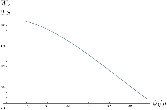
Figure 13: Left: Asymptotic volume complexity for charged solutions with $q=1$ at constant $T/\mu=0.15$. Right: Asymptotic volume complexity for uncharged solution at $T/\mu=0.25$.

The Lloyd bound Lloyd conjectures that the rate of computation of a quantum computer is bounded by a quantity which is proportional to the total energy of the system. In the context of holography, in Brown:2015lvg it was conjectured that the Lloyd bound for the complexity rate is saturated by the uncharged planar BH in AdS_d+1, i.e.

$$\frac{d\,C_{V}}{dt_{b}}\leq\frac{8\pi}{d-1}M\,,$$ (113)

where $M$ is the mass of the black hole. In the complexity=volume conjecture, the complexity rate is a monotonically increasing function of the time and so it is enough to check it at late time.

In our setting there is an extra subtlety, because the value of the black hole mass depends on the choice of the boundary conditions, see appendix D for details. We checked the Lloyd bound both for the Dirichlet and Neumann choices of boundary conditions, that for $d=3$ is

$$W_{V}\leq 4\pi M_{D,N}\,,$$ (114)

where $M_{D,N}$ are in eqs. (199,201). We find that the bound is satisfied in all the parameter space that we explored, see fig. 14 for some sample plots for fixed value of $\phi_{0}$. This is consistent with Yang:2019gce , who numerically checked the Lloyd bound in the case of zero sources (for which the Neumann and Dirichlet masses coincide).

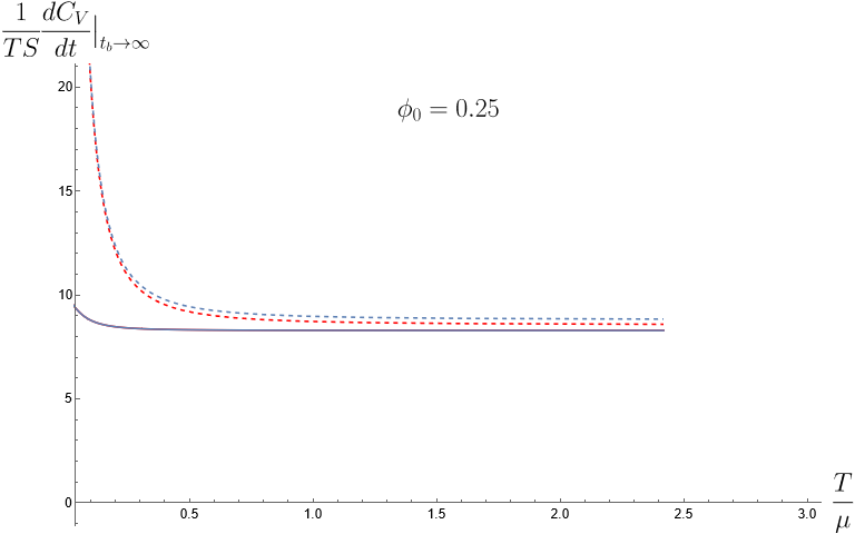
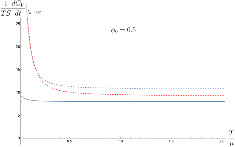
Figure 14: In these pictures, we show $W_{V}/(TS)$ in solid line, $(4\pi M_{D})/(TS)$ in blue dashed line and $(4\pi M_{N})/(TS)$ in red dashed line (see eqs. (110),(114)) as a function of $T/\mu$ for a fixed $\phi_{0}$. Left: neutral scalar. Right: charged $q=1$ scalar. The Lloyd bound is always satisfied for both the Dirichlet and the Neumann definition of mass.

3.5 Generalised volume functionals

A broader class of complexity duals were proposed in Belin:2021bga . In particular, a larger class of functionals was considered, i.e.

$$\hat{S}=\int d^{3}\sigma\,\sqrt{h}\,F(g_{\mu\nu},X^{\mu})\,,$$ (115)

where $F$ is a scalar function of the background metric and of the embedding $X^{\mu}(\sigma^{a})$ of the codimension-one surface. These functionals may provide an infinite class of alternative holographic definitions of complexity; the CV conjecture is recovered by setting $F$ equal to a constant.

If we consider a surface parameterized by $(\lambda,x,y)$ in our metric ansatz, we have that a functional of the form eq. (115) can be written as follows

$$\hat{S}=\int d\lambda\,\frac{a(z)}{z^{3}}\sqrt{-2\dot{v}\dot{z}e^{-\frac{\chi}{2}}-fe^{-\chi}\dot{v}^{2}}=\int d\lambda\,\hat{\mathcal{L}}\,,$$ (116)

where the function $a(z)$ can be found by evaluating $F(g_{\mu\nu},X^{\mu})$ on the surface.

In a similar way to eq. (95), due to translation invariance in $v$, we can again define the conserved quantity

$$E=-\frac{\partial\hat{\mathcal{L}}}{\partial\dot{v}}=\frac{a(z)}{z^{k}}\frac{\dot{z}\,e^{-\frac{\chi}{2}}+\dot{v}fe^{-\chi}}{\sqrt{-2\dot{v}\dot{z}e^{-\frac{\chi}{2}}-fe^{-\chi}\dot{v}^{2}}}\,.$$ (117)

As in eq (96), it is convenient to fix the $\lambda$ parameterization as follows

$${z^{3}}\sqrt{-2\dot{v}\dot{z}e^{-\frac{\chi}{2}}-fe^{-\chi}\dot{v}^{2}}=a(z)\,e^{-\frac{\chi}{2}}\,.$$ (118)

In this gauge, the conserved quantity $E$ takes the form

$$E=\dot{z}+\dot{v}fe^{-\chi/2}\,,\qquad\dot{v}=(E-\dot{z})\frac{e^{\frac{\chi}{2}}}{f}\,,$$ (119)

which, inserted back in (118) gives an effective potential as in eq. (98)

$$\dot{z}^{2}+V(z)=E^{2}\,,\qquad V(z)=-\frac{e^{-\chi}\,f\,a^{2}}{z^{6}}\,.$$ (120)

The details of complexity evolution depend crucially on the choice of $F(g_{\mu\nu},X^{\mu})$. Let us briefly discuss an example. Let us choose, as in the example explicitly discussed in Belin:2021bga , the following function

$$F(g_{\mu\nu},X^{\mu})=1+\kappa\,W_{\mu\nu\rho\sigma}W^{\mu\nu\rho\sigma}\,,$$ (121)

where $\kappa$ is a constant and $W_{\mu\nu\rho\sigma}$ is the spacetime Weyl tensor. In this case, we find

$$a=1+\kappa\,\frac{z^{4}}{12}\left(2f^{\prime\prime}-3f^{\prime}\chi^{\prime}+f(\chi^{\prime})^{2}-2f\chi^{\prime\prime}\right)\,.$$ (122)

If we specialize to the RN back hole case as in eq. (24), we find:

$$a=1+\kappa\,\frac{12z^{6}\left(\left(z_{c}+z_{h}\right)\left(z_{c}^{2}+z_{h}^{2}\right)-2z\left(z_{c}z_{h}+z_{c}^{2}+z_{h}^{2}\right)\right){}^{2}}{z_{c}^{6}z_{h}^{6}}\,.$$ (123)

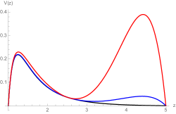
Figure 15: Examples of potentials $V(z)$ the RN black solution for with $z_{h}=1$, $z_{c}=5$. In the black curve, we choose the volume functional, i.e. $F=1$. In the blue and red curves, we choose the functional in eq. (121) with $\kappa=0.0003$ and $\kappa=0.003$, respectively.

We plot some examples of potentials in figure 15. In these cases the potential in eq. (120) has two maxima. Each of these maxima correspond to an extremal surface of the given functional which is attached to the boundary at a time $t_{b}\to\infty$.

This shows that, changing $F(g_{\mu\nu},X^{\mu})$, for a given value of the time we can have multiple extremal surfaces. The asymptotic complexity rate for each of the extremal surfaces is proportional to the value of $\sqrt{V(z)}$ evaluated on each of the maxima. With a generic choice of the parameter $\kappa$, we expect that, in the hairy black hole case, the extremal surface remains generically far from the would be Cauchy horizon. It would be interesting to study other choices of $F(g_{\mu\nu},X^{\mu})$ in a more systematic way. We leave this as a topic for further investigation.

4 Action complexity

To compute the action complexity we must first identify the Wheeler-DeWitt (WDW) patch Brown:2015bva , which is given by the union of all the spatial slices that can be attached to the left and right boundaries at some given pair of times $t_{L}$ and $t_{R}$. The Killing vector corresponding to a translation in $t$ in the metric (18) shifts

$$t_{L}\to t_{L}+\delta t\,,\qquad t_{R}\to t_{R}+\delta t\,.$$ (124)

For this reason, if we take the left and the right time translation in opposite direction, the thermofield double state is time-independent. In order to study the time dependence of the complexity of the thermofield double, we take as boundary conditions for the WDW patch

$$t_{L}=t_{R}=\frac{t_{b}}{2}\,.$$ (125)

The boundary of the WDW patch can be obtained by sending null rays from the left and right boundary.

Various shapes of the WDW region are possible. If the future light rays meet at a point we have a future joint, otherwise the future light rays end in the singularity and thus we have a space-like side of the WDW. The same is true for the past light rays so in total we have four possible shapes: the diamond ​​ , a five-sides polygon with one side on the singularity of the future ​​ or the past ​​ , or a six- sides polygon with sides on both singularities ​​ .

Once the WDW patch is obtained for a given boundary time $t_{b}$, we need to compute the action Lehner:2016vdi which is given by the sum of the following contributions

$$I_{\rm WDW}=I_{\rm V}+I_{\rm GHY}+I_{\rm J}+I_{\rm b}+I_{\rm ct}\,,$$ (126)

where $I_{\rm V}$ is the bulk actions in eq. (14), $I_{\rm GHY}$ is the Gibbons-Hawking-York boundary term eq. (207), $I_{\rm J}$ is the joint term (212), $I_{\rm b}$ is the null boundary term (216) and $I_{\rm ct}$ its counter term (218). Details on how to compute these four terms are given in appendix E. We will always compute the derivative of the action with respect the boundary time $\frac{dI_{\rm WDW}}{dt_{b}}$. This removes various UV divergences present in $I_{\rm WDW}$.

In addition to the gravitational constant $G$, the action (126) contains a scale $L_{\rm ct}$ which is needed in a counterterm that restores the reparameterization invariance of the action. This term was introduced in Lehner:2016vdi with the motivation to remove an ambiguity in the parameterization of the null hypersurfaces which delimit the WDW patch. In many static situations, such as in Carmi:2017jqz , the asymptotic complexity rate at $t_{b}\to\infty$ is independent on $L_{ct}$, which affects only the action rate during a finite transient period. In out-of-equilibrium situations, such as Vaidya spacetime, the counterterm is important in order to reproduce many expected properties of complexity, such as the late-time growth and the switchback effect Chapman:2018dem ; Chapman:2018lsv . The counterterm scale introduces an ambiguity in defining holographic complexity that could be related to the details of how complexity is defined in the dual field theory, such as the reference state or the choice of gates.

In order to evaluate the action of the WDW patch, it is convenient to introduce the tortoise coordinate

$$z^{*}(z)=\int_{0}^{z}\frac{d\tilde{z}}{f(\tilde{z})}e^{\frac{\chi(\tilde{z})}{2}}\,,$$ (127)

in which the radial-time part of the metric is conformally flat

$$ds^{2}=\frac{1}{z^{2}}\left(fe^{-\chi}(-dt^{2}+(dz^{*})^{2})+dx^{2}+dy^{2}\right)\,,$$ (128)

and the coordinates $u$ and $v$

$$v=t-z^{*}\,,\qquad u=t+z^{*}\,.$$ (129)

The time dependence of the action complexity depends on the type of Penrose diagram that we are considering, which can have a singularity with upper bending (type $U$) or lower bending (type $D$). It is useful to introduce a quantity to discriminate the two kinds of behaviour. An ingoing null geodesic which leaves the boundary at $t_{b}=0$ reaches the singularity at a time $t_{\infty}$ given by

$$t_{\infty}=z^{*}(\infty)=\int_{0}^{\infty}\frac{e^{\frac{\chi}{2}}}{f}d\tilde{z}\,,$$ (130)

which is a convergent integral at $z\to\infty$, as can be shown using the asymptotic Kasner behaviour in eq. (32). This shows that the integral is converging at large $z$. If the quantity $t_{\infty}$ is positive, the solution is of type $D$. Instead, if $t_{\infty}$ is negative, the solution is of type $U$. In both cases, there is a critical boundary time $t_{c}$ at which the structure of the WDW patch changes in a discontinuous way.

4.1 RN case

The time dependence of action complexity for the RN black hole was studied in Carmi:2017jqz . We briefly review their results in appendix F, where we give a closed-form expression for the time dependence of the complexity. In general, the details of the evolution during the transient time range area function the counterterm scale $L_{\rm ct}$. The complexity rate at late time is instead independent of $L_{\rm ct}$.

Nearby the extremal limit, at small $T/\mu$, we have that the time dependence of the rate of the action complexity is a smooth monotonic function of the time, and it is at first approximation independent of the counterterm scale $L_{\rm ct}$. By expanding the results in Carmi:2017jqz (see appendix F.1) we find the compact expression

$$\frac{dI}{dt_{b}}\approx\frac{3\,V_{0}}{4\pi G}\frac{z_{c}-z_{h}}{z_{h}^{4}}\tanh\frac{3t_{b}(z_{c}-z_{h})}{2z_{h}^{2}}\,.$$ (131)

For a comparison with numerical results, see the top panel of figure 16.

As we increase $T/\mu$, the qualitative features of the plot change. For $T/\mu\to\infty$, the Schwarzschild case must be reproduced. In this case, the complexity rate is zero up to the critical time $\hat{t}_{c}$ in eq (2.9) of Carmi:2017jqz

$$\hat{t}_{c}=\frac{1}{2T}\frac{1}{\sqrt{3}}=\frac{2\pi}{3\sqrt{3}}z_{h}\approx 1.21z_{h}\,.$$ (132)

where $T$ is the temperature $T=3/(4\pi z_{h})$. In appendix F.2 we check that this is indeed the case, by studying the $z_{c}/z_{h}\to\infty$ of the RN case. Just after $\hat{t}_{c}$, the rate drops to $-\infty$ in a discontinuous way, and after that raises to approach a positive constant at late time.

At large but finite $T/\mu$, we have that the action rate is still to a good approximation constant up to a timescale $t_{b}\approx\hat{t}_{c}$. Then, there is a sudden drop of the action rate to a large negative value (which in the limit $T/\mu\to\infty$ tends to $-\infty$). After that the action rate raises and approaches a positive constant at $t_{b}\to\infty$. Figure 16 shows and example of this behavior from the numerical solution.

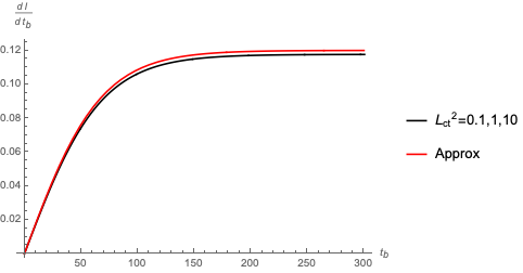
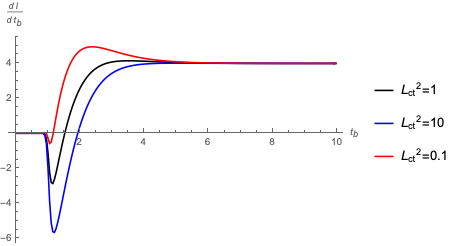
Figure 16: Action complexity rate as a function of time for some examples of RN case, with $V_{0}/(16\pi G)=1$. Top: almost extremal case with $T/\mu=1.4\cdot 10^{-3}$, $\rho=3.43$ and $z_{h}=1$. The approximate analytical expression in eq. (131) in red is compared with numerical one, in black. In the scale of the plot, the curves with ${L}_{\rm ct}^{2}=0.1,1,10$ all coincide with the black curve. Bottom: case with $T/\mu=0.28$, $\rho=0.8$ and $z_{h}=1$ (for various ${L}_{\rm ct}^{2}$).

At late time, from a direct calculation it follows that the bulk contribution in eq. (228) vanishes, i.e. ${dI_{V}}/{dt_{b}}\approx 0$. Also, we can approximate eq. (229) as

$$\frac{dI_{J}}{dt_{b}}\approx\frac{V_{0}}{8\pi G}\left(\left.\frac{f_{\rm RN}^{\prime}}{2z^{2}}\right|_{z=z_{c}}-\left.\frac{f_{\rm RN}^{\prime}}{2z^{2}}\right|_{z=z_{h}}\right)\,.$$ (133)

Defining a formal temperature $T_{c}$ and an entropy $S_{c}$ computed on the Cauchy horizon

$$T_{c}=-\frac{1}{4\pi}f_{\rm RN}^{\prime}(z_{c})=-\frac{(z_{c}-z_{h})(3z_{h}^{2}+2z_{c}z_{h}+z_{c}^{2})}{4\pi z_{c}z_{h}^{3}}\,,\qquad S_{c}=\frac{1}{4G}\frac{V_{0}}{z_{c}^{2}}\,,$$ (134)

the action rate at late time is

$$W_{A}=\lim_{t_{b}\to\infty}\frac{dI_{\rm WDW}}{dt_{b}}=\frac{V_{0}}{4\pi G}\frac{z_{c}^{3}-z_{h}^{3}}{z_{c}^{3}z_{h}^{3}}=T\,S\,-T_{c}\,S_{c}\,,$$ (135)

where $T$ and $S$ are the RN temperature and entropy in eqs (27) and (28). A plot of the asymptotic action rate is shown on the left hand side of figure 17. On the right hand side of the same figure, we compare the action and the volume rates for different $T/\mu$.

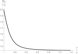
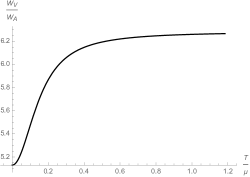
Figure 17: Left: Plot of ${W_{A}}/{TS}$ as a function of $T/\mu$ for the RN solution. Right: Ratio between the asymptotic CV and the asymptotic CA rate as a function of $T/\mu$ for the RN solution. Combining eqs. (111), (112) and (135), we find that for $T/\mu\to\infty$ we have $W_{V}/W_{A}=2\pi$, while for $T/\mu\to 0$ we have $W_{V}/W_{A}=2\pi\sqrt{2/3}$. This is in agreement with numerical calculations for generic $T/\mu$.

4.2 Type $D$

This case corresponds to a singularity with a lower bending and to $t_{\infty}>0$. Here the WDW starts at $t_{b}=0$ in the shape ​​ , with two sides on the past and future singularity. There is a critical time:

$$t_{c}=2z^{*}(\infty)=2t_{\infty}\,.$$ (136)

For $t_{b}<t_{c}$, the WDW remains hexagonal, see figure 1 on the left. In this case the complexity rate is zero, because the time dependence contribution from regions $1$ and $3$ in figure turns out to cancel each other, and the contribution from region $2$ is time independent. See appendix G.1 for the details of the calculation. The same cancellation is present also for the Schwarzschild case Carmi:2017jqz .

At $t_{b}=t_{c}$ the shape becomes ​​ with the lower tip touching the past singularity. For $t_{b}>t_{c}$ the shape remains ​​ with only one side at the future singularity. See figure 1 on the right. Here the complexity rate is non zero and has a non trivial time dependence on $t_{b}$. First of all, we should find the $z_{m1}$ of the lower tip of the WDW as a function of $t_{b}$. For $t_{b}=t_{c}$, we have $z_{m1}\rightarrow\infty$ since it is touching the past singularity. For $t_{b}\rightarrow\infty$, we have $z_{m1}=z_{h}$. For generic time $t>t_{c}$, we can find $z_{m1}(t_{b})$ by inverting the equation:

$$z^{*}(z_{m1})=\frac{t_{b}}{2}\,;$$ (137)

it is the same as the equation (226) for the RN case, but now only the lower tip is relevant. For the complexity rate we should evaluate three contributions

$$\frac{dI}{dt_{b}}=\frac{d\,I_{V}}{dt_{b}}+\frac{d\,I_{\rm GHY}}{dt_{b}}+\frac{d\,(I_{J}+I_{\rm ct})}{dt_{b}}\,.$$ (138)

A detailed derivation is provided in appendix G.3. The bulk contribution is given by

$$\frac{d\,I_{V}}{dt_{b}}=\frac{V_{0}}{16\pi G_{N}}\int^{\infty}_{z_{m1}}dz\,s(z)\,,$$ (139)

where $s(z)$ is given by eq. (206). The GHY contribution is a constant and gives:

$$\frac{dI_{\rm GHY}}{dt_{b}}=\frac{V_{0}}{16\pi G}\lim_{z\to\infty}A(z)\,,$$ (140)

where $A(z)$ is given by eq. (211). Using the asymptotic Kasner solution in eq. (32) in the expression (211) we find

$$A(\infty)=f_{0}e^{-\frac{\chi_{0}}{2}}(3+\alpha^{2})\,.$$ (141)

The joints and counterterm contributions are

$$\frac{d(I_{J}+I_{\rm ct})}{dt_{b}}=\frac{V_{0}}{16\pi G}\left\{fe^{-\frac{\chi}{2}}\left[\frac{2}{z^{3}}\log\left(-4f\,{L}_{\rm ct}^{2}\right)-\frac{1}{z^{2}}\frac{d}{dz}\left(\log\frac{-fe^{-\chi}}{z^{2}}\right)\right]\right\}_{z=z_{m1}}$$ (142)

Examples of total complexity rate as function of time are shown in figure 18.

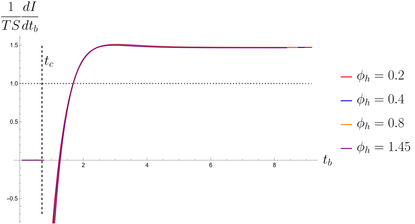
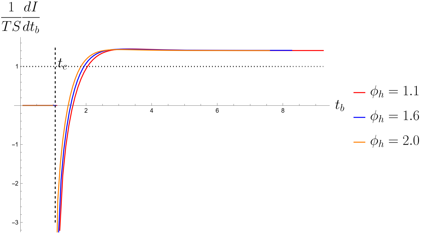
Figure 18: Time dependence of the action complexity rate in various type D examples. Top: $q=0$ and $\rho=2$. Down: $q=1$ and $\rho=0.6$. In these examples we set $z_{h}=1$ and ${L}_{\rm ct}=1$.

It is interesting to investigate more in detail the behaviour of the complexity rate nearby the critical time $t_{c}$ in eq. (136). Before $t_{c}$, the action rate vanishes. Just after the critical time $t_{c}$, the joint inside the past horizon sits nearby the singularity, in the Kasner region at $z_{m}\rightarrow\infty$. Using the approximations in eq. (32), we find the negative log divergence in the joint part of the action rate

$$\frac{dI_{J}}{dt_{b}}\approx-\frac{V_{0}}{8\pi G}A(\infty)\,\log z_{m}\,.$$ (143)

where $A(\infty)$ is given in eq. (141). Combining eq. (247) with the $z\to\infty$ behaviour in (32), we obtain

$$\frac{dz_{m1}}{dt_{b}}\approx\frac{-f_{0}e^{-\frac{\chi_{0}}{2}}\,z_{m1}^{3}}{2}\,.$$ (144)

Integrating this differential equation nearby critical time (where $\Delta t_{b}=t_{b}-t_{c}>0$), we find:

$$z_{m1}=\frac{1}{\sqrt{f_{0}e^{-\frac{\chi_{0}}{2}}\Delta t_{b}}}\,,$$ (145)

which gives the following behaviour as a function of time

$$\frac{dI_{J}}{dt_{b}}\approx\frac{V_{0}}{16\pi G}A(\infty)\,\log\Delta t_{b}\,.$$ (146)

So, for small $\Delta t_{b}>0$ the rate diverges $\to-\infty$. This divergence is visible in the type $D$ example of figure 18 on as $t\to t_{c}^{+}$. The divergence at $t_{b}=t_{c}$ is similar to the one that we have for the Schwarzschild case for $t_{b}=\hat{t}_{c}$ in eq. (132).

4.3 Type $U$

This case corresponds to $t_{\infty}<0$ and to a singularity with an upper bending. This situation is realised in the limit of $\phi_{h}\to 0$, which is closer to the unperturbed RN solution. Here the WDW starts at $t_{b}=0$ in the shape ​​ . There is a critical time, for which the WDW changes shape, given by

$$t_{c}=-2z^{*}(\infty)=-2t_{\infty}\,.$$ (147)

As we approach the limit $\phi_{h}\to 0$, the critical time $t_{c}$ goes to infinity. In appendix H we perform an analytic estimate of the divergence of the critical time, which give the result

$$t_{c}=O\left(\frac{1}{\phi_{h}^{2}}\right)\,.$$ (148)

This is consistent with the numerical calculations, see figure 19.

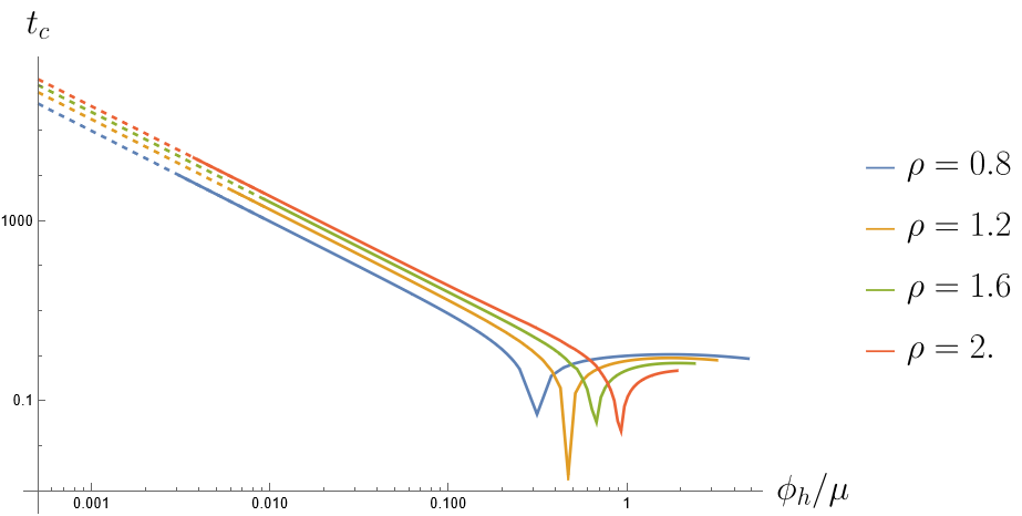
Figure 19: Critical time for the $q=0$ case as function of $\phi_{h}$, for several $\rho$ and $z_{h}=1$. For each curve, the minimum in $t_{c}$ separates the solutons of types U and D. Dashed lines are extrapolations following the law $t_{c}={\rm const.}\times\left(\phi_{h}/\mu\right)^{-2.003_{3}}$.

For $t<t_{c}$, , the WDW is a diamond, see figure 2 on the left for an example. It is important to know first the coordinate of the two joints inside the horizons as a function of the boundary time $t_{b}$. Let us denote respectively by $z_{m1}$ and $z_{m2}$ the coordinates of the joints inside the white and the black hole horizons. They can be found by solving the equations

$$z^{*}(z_{m1})=\frac{t_{b}}{2}\,,\qquad z^{*}(z_{m2})=-\frac{t_{b}}{2}\,.$$ (149)

For the complexity rate we should evaluate two contributions:

$$\frac{dI}{dt_{b}}=\frac{d\,I_{V}}{dt_{b}}+\frac{d(I_{J}+I_{\rm ct})}{dt_{b}}\,.$$ (150)

See appendix G.2 for details. The bulk contribution is

$$\frac{d\,I_{V}}{dt_{b}}=\frac{V_{0}}{16\pi G_{N}}\int^{z_{m2}}_{z_{m1}}s(z)dz\,,$$ (151)

$s(z)$ is given by eq. (206). The joints and the counterterm give

$$\frac{d(I_{J}+I_{\rm ct})}{dt_{b}} = \frac{V_{0}}{16\pi G}\left(\left\{fe^{-\frac{\chi}{2}}\left[\frac{2}{z^{3}}\log\left(-4f\,{L}_{\rm ct}^{2}\right)-\frac{1}{z^{2}}\frac{d}{dz}\left(\log\frac{-fe^{-\chi}}{z^{2}}\right)\right]\right\}_{z=z_{m1}}\right.$$ (152)

$$-\left.\left\{fe^{-\frac{\chi}{2}}\left[\frac{2}{z^{3}}\log\left(-4f\,{L}_{\rm ct}^{2}\right)-\frac{1}{z^{2}}\frac{d}{dz}\left(\log\frac{-fe^{-\chi}}{z^{2}}\right)\right]\right\}_{z=z_{m2}}\right)$$

At $t_{b}=t_{c}$ the shape is still ​​ with the higher tip touching the future singularity. For $t_{b}>t_{c}$ the shape becomes ​​ with only one side at the future singularity. See figure 2 on the right for an example. For $t>t_{c}$, only $z_{m1}$ exists and can be found solving the first of (149). During this stage, the structure of WDW patch is the same of case $D$ and also the expression for the complexity rate eqs. (138)-(142). Examples of complexity rate in case $U$ for different $\phi_{h}$ as function of time are given in figure 20. In figure 21 we show a plot of total complexity rate for the uncharged case as a function of choice of ${L}_{\rm ct}$.

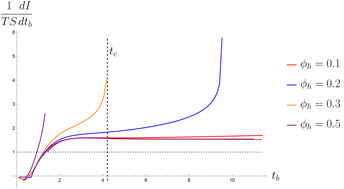
Figure 20: Time dependence of the action complexity rate in various type U examples for various $\phi_{h}$, with $q=0$, $z_{h}=1$ and ${L}_{\rm ct}=1$.

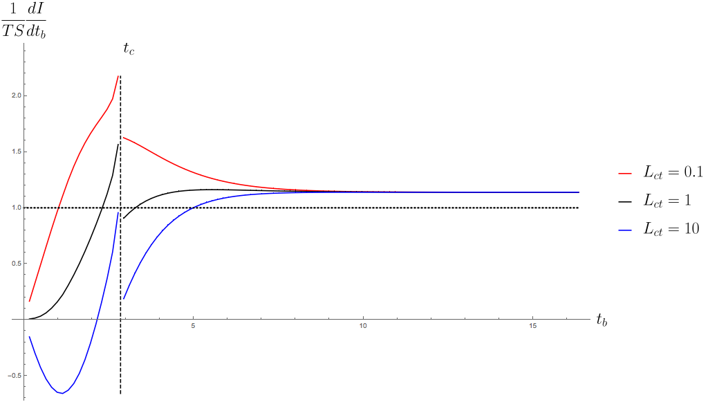
Figure 21: Time dependence of the action complexity rate as a function of $t_{b}$ for various ${L}_{\rm ct}$ with $q=0$, $\phi_{h}=0.7$, $z_{h}=1$ and $\rho=2.2$.

It is interesting to investigate the behaviour of the complexity rate nearby the critical time in eq. 147. Just before the critical time $t_{c}$ , as the joint inside the future horizon approaches the singularity, the action rate get a positive divergent contribution

$$\frac{dI_{J}}{dt_{b}}\approx\frac{V_{0}}{8\pi G}\,A(\infty)\,\log z_{m2}\,,$$ (153)

where $A(\infty)$ is given in eq. (141). Just after $t_{c}$ there is no divergence in the rate. Combining eq. (240) with the $z\to\infty$ behaviour in (32), we obtain

$$\frac{dz_{m2}}{dt_{b}}\approx\frac{f_{0}e^{-\frac{\chi_{0}}{2}}\,z_{m2}^{3}}{2}\,.$$ (154)

Following the same steps as for case $D$, we obtain

$$z_{m1}=\frac{1}{\sqrt{-f_{0}e^{-\frac{\chi_{0}}{2}}\Delta t_{b}}}\,,$$ (155)

which gives, as a function of time

$$\frac{dI_{J}}{dt_{b}}\approx-\frac{V_{0}}{16\pi G}A(\infty)\,\log(-\Delta t_{b})\,.$$ (156)

So, for small $\Delta t_{b}<0$ the rate diverges $\to\infty$. This divergence is visible in the type $U$ example of figure 20 on as $t\to t_{c}^{-}$.

The divergence of the action complexity rate at the critical time $t_{c}$ then is determined by the quantity $A(\infty)$ in eq. (141), which contains the parameters of the metric in the $z\to\infty$ Kasner regime, defined in eq. (32). So one may think that the coefficient of the logarithmic divergence of the complexity rate at $t_{b}=t_{c}$ is directly related to the Kasner exponent in the black hole interior. This does not seem to be the case, at least in the regime of small $\phi_{h}$. In particular, let us distinguish to cases:

• for $q=0$ and $\phi_{h}\to 0$, we have that $A(\infty)$ is not directly sensitive to the Kasner parameter $\alpha$ (which in this limit tends to infinity), but to a quantity that can be defined in term of the unperturbed RN geometry. This can be shown combining eqs. (141) and (86), which give

  $$A(\infty)=\frac{(z_{c}-z_{h})(z_{c}^{2}+2z_{c}z_{h}+3z_{h}^{2})}{z_{c}^{3}z_{h}^{3}}=-\frac{16\pi G}{V_{0}}T_{c}S_{c}\,,$$ (157)

  where $T_{c}$ and $S_{c}$ are the formal temperature and entropy computed on the Cauchy horizon of the RN solution, see eq. (134).

• for $q\neq 0$ and $\phi_{h}\to 0$, we have that $A(\infty)$ vanishes. This can be checked from eq. (85) and eq. (87) we find that for the final Kasner region $f_{0}e^{-\chi_{0}/2}\to 0$. Also, as the limit $\phi_{h}\to 0$ is approached, $\alpha$ oscillates many times, remaining finite. From from eq. (141) we find

  $$\lim_{\phi_{h}\to 0}A(\infty)=\lim_{\phi_{h}\to 0}f_{0}e^{-\frac{\chi_{0}}{2}}(3+\alpha^{2})=0\,.$$ (158)

  So in this limit the divergence of the complexity rate at $t_{b}=t_{c}$ tends to disappear.

In figure 22 we plot for the complexity rate in some type U examples, with charged scalar field $q=1$.

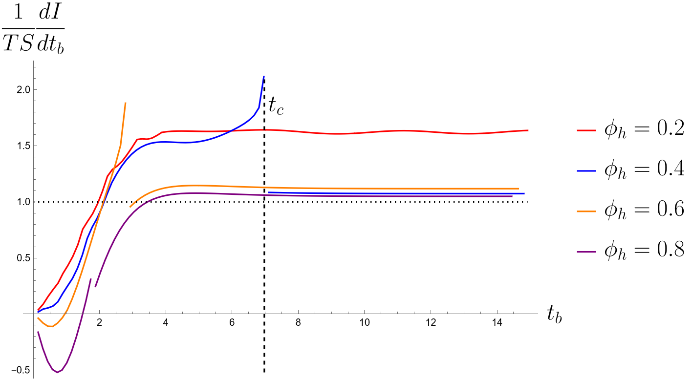
Figure 22: Complexity rate for $q=1$ and $\rho=2$ as a function of $t_{b}$ for various values of $\phi_{h}$ and ${L}_{\rm ct}=1$. The divergence in the complexity rate occurs at $t_{b}=t_{c}$ and is shown here for a particular value of $\phi_{h}=0.4$. Type U cases.

4.4 Asymptotic complexity rate

In the late time limit $z_{m1}\to z_{h}$ and the contribution in eq. (142) is

$$\left.\frac{d(I_{J}+I_{ct})}{dt_{b}}\right|_{t_{b}\to\infty}=-\frac{V_{0}}{8\pi G}\left\{\frac{e^{-\frac{\chi}{2}}}{2z^{2}}f^{\prime}\right\}_{z=z_{h}}=TS\,,$$ (159)

where $T$ ans $S$ are respectively the temperature and the entropy

$$T=-\frac{1}{4\pi}f^{\prime}(z_{h})e^{-\frac{\chi(z_{h})}{2}}\,,\qquad S=\frac{1}{4G}\frac{V_{0}}{z_{h}^{2}}\ .$$ (160)

We can write the asymptotic action rate including also the volume term as

$$W_{A}=\lim_{t_{b}\to\infty}\frac{dI_{\rm WDW}}{dt_{b}}=TS+\frac{V_{0}}{16\pi G}\left(A(\infty)+\int^{\infty}_{z_{h}}\,s(z)\,dz\right)\,.$$ (161)

For small $\phi_{h}$, the bulk contribution in eq. (161) tends to zero. To show this, let us separate the bulk integral in to pieces: first, the integral of $s(z)$ up to the Cauchy horizon of the undeformed RN. This integral is exactly zero if evaluated on the RN solution, and so it is approximately zero for $\phi_{h}\to 0$:

$$\int_{z_{h}}^{z_{c}}s(z)\,dz=0\,.$$ (162)

Then, there is the integral for $z>z_{c}$, which, using eq. (206), is given by the approximation:

$$\int_{z_{c}}^{\infty}s(z)\,dz=\int_{z_{c}}^{\infty}\frac{e^{-\frac{\chi}{2}}}{z^{4}}\left(-6-2\phi^{2}+\frac{1}{2}\tilde{\rho}^{2}z^{4}\right)dz\,.$$ (163)

This integral is converging because at large $z$

$$s(z)\approx\frac{1}{2}e^{-\frac{\chi_{0}}{2}}\frac{-12+z^{4}\rho^{2}-8\alpha^{2}(\log z)^{2}}{z^{4+\alpha^{2}}}$$ (164)

and $\alpha^{2}>1$ for the final Kasner region. Moreover, for $\phi_{h}\to 0$ we have that $\chi$ tends to $\infty$ very fast for $z>z_{c}$, and so the integral (163) tends to zero.

We give now an analytic expression for the asymptotic complexity rate in the $\phi_{h}\to 0$ limit. We distinguish two case:

• For $q=0$ and in the $\phi_{h}\to 0$ limit, we have that the contribution due to $A(\infty)$ reproduces the contribution of the second joint $z_{m2}$ for the RN, see eq. (157). So, for $q=0$ and in the $\phi_{h}\to 0$ limit, we recover the asymptotic complexity rate of the RN solution eq. (135), i.e.

  $$W_{A}=W_{A}^{(RN)}=T\,S\,-T_{c}\,S_{c}\,,$$ (165)

• For $q\neq 0$ and $\phi_{h}\to 0$, from eq. (158) that the contribution due to $A(\infty)$ vanishes. In this case, we find

  $$W_{A}=TS\,.$$ (166)

For generic $\phi_{h}$, the asymptotic complexity rate can be computed numerically using eq. (161). We numerically checked that in the $\phi_{h}\to 0$ limit the analytic expressions (165) and (166) are reproduced, see figure 23 for some illustrative plots.

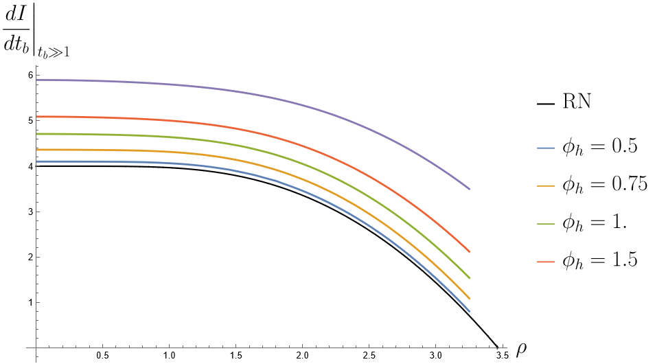
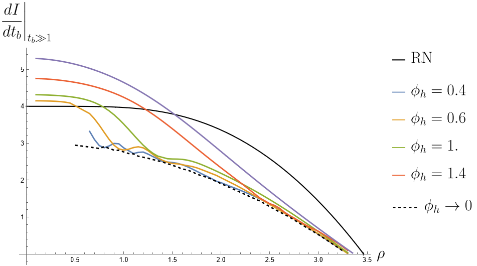
Figure 23: Asymptotic complexity rate $W_{A}$ as function of $\rho$ for a few values of $\phi_{h}$, with $16\pi G=1$, $V_{0}=1$ and $z_{h}=1$. For comparison, in black we show $W_{A}$ for the RN black hole. Left: neutral scalar case. In this case $W_{A}$ approaches the RN limit for $\phi_{h}\to 0$. Right: charged scalar case with $q=1$. In this case $W_{A}$ approaches $TS$, which is shown in the dashed line, in the $\phi_{h}\to 0$ limit.

We show the result of a scan in the parameter space of the model in figure 24. This confirms the expectation that the order of magnitude of $W_{A}$ is $TS$. In figure 25 we show the dependence of $W_{A}$ on $\phi_{0}/\mu$ at constant $T/\mu$. For $T/\mu=0.15$, we see that $W_{A}$ has an interesting oscillatory behavior as a function of $\phi_{0}/\mu$. The amplitude of these oscillations vanishes for $\phi_{0}\to 0$. It is tempting to associate these oscillations to the Josephson oscillations of the scalar field, since these do not appear in the neutral scalar case, where the solution profile of the scalar field has no oscillations.

Figure 24: Left: neutral scalar case $q=0$. Right: charged scalar case with $q=1$. Red points denote type D solutions, black points denote type U solutions. The white region is not covered by our numerics.

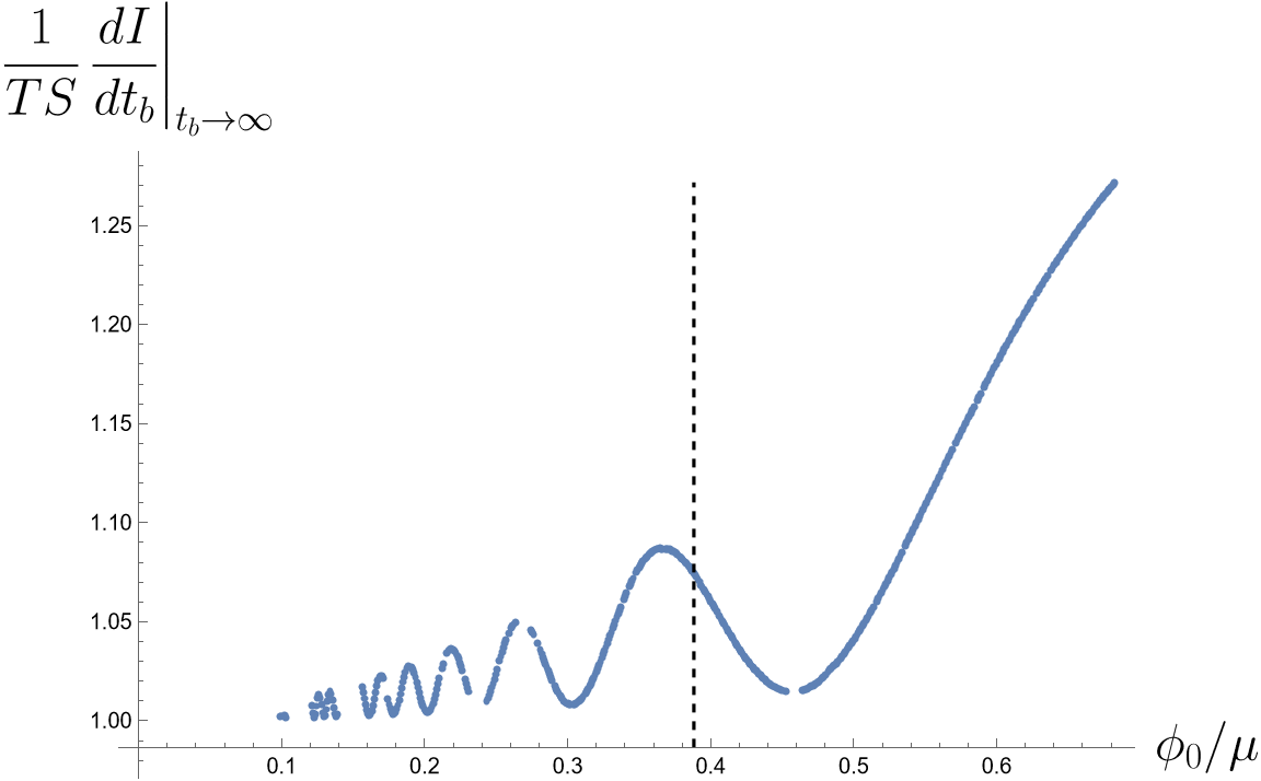
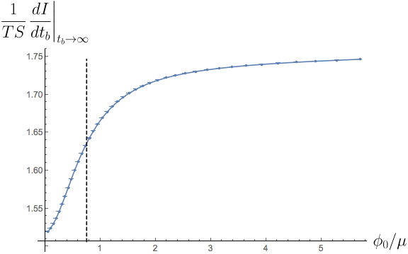
Figure 25: Left: Asymptotic action complexity for charged solutions with $q=1$ at constant $T/\mu=0.15$. The dashed line corresponds to the Temperature at which the solution changes type. Right: Asymptotic action complexity for uncharged solution at $T/\mu=0.25$.

It has been conjectured Brown:2015lvg that the Lloyd bound is saturated by the uncharged planar BH in AdS_d+1, i.e.

$$\frac{d\,I_{WDW}}{dt_{b}}\leq{2M}\,,$$ (167)

where $M$ is the mass of the BH. This bound in eq. (167) is violated by the action conjecture Carmi:2017jqz ; Yang:2017czx , because the asymptotic value (which is supposed to saturate the bound) is approached from above. In the examples studied in this paper, we have that for type $U$ black holes the complexity rate approaches infinity at critical time, and so this also provides another example of violation of the bound.

One may wonder if a weaker version of the Lloyd bound holds for the asymptotic complexity rate $W_{A}$, i.e.

$$W_{A}\leq 2\,M\,.$$ (168)

Violations to the bound of eq. (168) have been previously found in Couch:2017yil ; Swingle:2017zcd ; An:2018xhv ; Alishahiha:2018tep ; Mahapatra:2018gig ; Babaei-Aghbolagh:2021ast ; Avila:2021zhb . In our model, we checked that the bound given by eq. (168) holds in all the parameter space that we explored, with both choices $M=M_{D},M_{N}$ corresponding to Dirichlet and Neumann boundary conditions. See figure 26 for some sample plot.

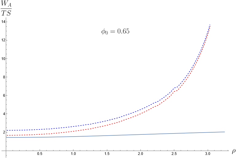
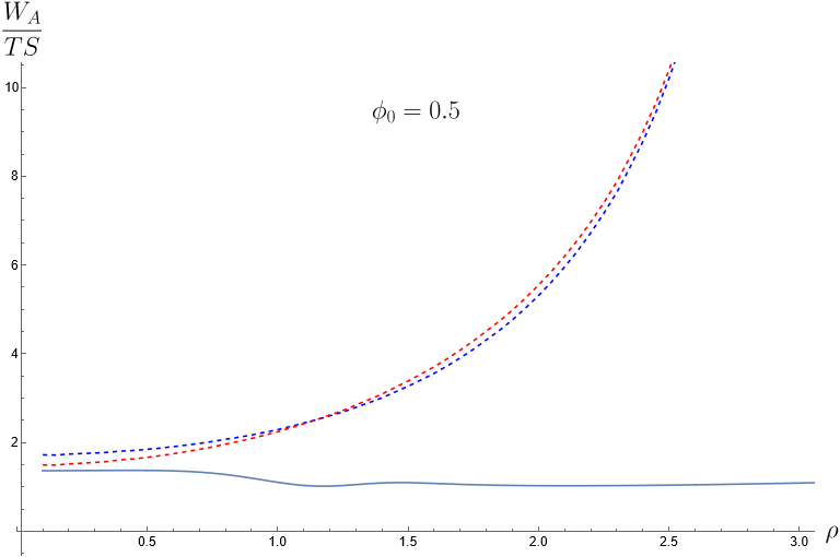
Figure 26: In these pictures, we show $W_{A}/(TS)$ in solid line, $(2M_{D})/(TC)$ in dashed blue line and $(2M_{N})/(TS)$ in dashed red line (see eqs. (161) and (168)) as a function of $\rho$ for a fixed $\phi_{0}$ and $z_{h}=1$. Left: neutral scalar. Right: charged $q=1$ scalar.

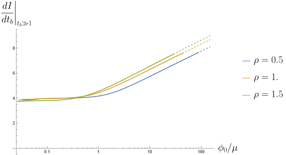
Figure 27: Asymptotic value of complexity at late time as function of the scalar source, for $z_{h}$. The dashed lines are extrapolations following the law $\left.\frac{dI}{dt_{b}}\right|_{t_{b}\gg 1}={\rm const.}+0.88_{1}\log\tfrac{\phi_{0}}{\mu}$.

We see from figure 27 that, for large $\phi_{0}/\mu$ the asymptotic action complexity rate has a logarithmic dependence on $\phi_{0}/\mu$ for fixed values of $\rho$ and $z_{h}$.

Appendix A Conservation of electric flux in the $q=0$ case

From Stokes theorem, we have

$$\int_{\Sigma}D_{\beta}F^{\alpha\beta}n_{\alpha}\,\sqrt{|h|}d^{3}y=\int_{\partial\Sigma}F^{\alpha\beta}\,n_{[\alpha}r_{\beta]}\sqrt{\sigma}d^{2}\theta$$ (169)

where $n^{\alpha},r^{\beta}$ are unit normals, ${\Sigma}$ denotes a codimension 1 submanifold, $\partial{\Sigma}$ denotes the boundary of $\Sigma$, which is codimension 2, and $\sqrt{|h|}d^{3}y$ and $\sqrt{\sigma}d^{2}\theta$ are the induced metric measures on codimension $1$ and $2$ submanifolds. For $q=0$ we have from Maxwell eqs. that $D_{\beta}F^{\alpha\beta}=0$. Then, the right hand side of eq. (169) is zero if integrated on a closed boundary $\partial\Sigma$. The only non-vanishing component of the gauge field strength is

$$F^{tz}=a^{\prime}(z)e^{\chi}z^{4}\,,$$

Using the unit normals and codimension 2 measure

$$n_{\alpha}=(1,0,0,0)\frac{\sqrt{|f|}e^{-\frac{\chi}{2}}}{z}\,,\qquad r_{\alpha}=(0,1,0,0)\frac{1}{z\sqrt{|f|}}\,,\qquad\sqrt{\sigma}d^{2}\theta=\frac{dx\,dy}{z^{2}}\,,$$

we get

$$a^{\prime}(z)e^{\frac{\chi}{2}}={\rm constant}=-\rho\,.$$ (170)

Appendix B Numerical techniques

For the neutral scalar case, we solve the system in eq. (50). Introducing both an IR and a UV cutoff, $z_{\rm max}$ and $z_{\epsilon}$ respectively, we then choose a value $z_{0}>z_{h}$ and split the full domain in two parts, $(z_{\epsilon},z_{0})$ and $(z_{0},z_{\rm max})$. We solve the problem in the small-$z$ regime imposing at the horizon

$$f(z_{h}) =0\,, \chi(z_{h})=\chi_{h}\,,$$

$$\phi(z_{h}) =\phi_{h}\,, \phi^{\prime}(z_{h})=-\frac{8\phi_{h}}{z_{h}\left(\rho^{2}z_{h}^{4}-4\phi_{h}^{2}-12\right)}\,.$$ (171)

The parameter $\chi_{h}$ is not physical. Once a solution is found, it can be removed by a reparameterization of the time coordinate $t$ at infinity. We can define

$$\hat{\chi}_{h}=\chi_{h}-\chi(0)\,.$$ (172)

Then, solving again with an initial condition $\chi(z_{h})=\hat{\chi}_{h}$, we can find the solution with the usual normalization of the time coordinate, where $\chi(0)=0$.

To determine the solution for the charged scalar case we take the full system of equations (20). We again split the full domain in two parts, $(z_{\epsilon},z_{0})$ and $(z_{0},z_{\rm max})$. We solve the system in the small-$z$ regime imposing at the horizon

$$f(z_{h}) =0\,, \chi(z_{h})=\chi_{h}\,,$$

$$a(z_{h}) =0\,, a^{\prime}(z_{h})=a_{1}\,,$$

$$\phi(z_{h}) =\phi_{h}\,, \phi^{\prime}(z_{h})=\frac{8\phi_{h}}{z_{h}\left(-a_{1}^{2}e^{\chi_{h}}z_{h}^{4}+4\phi_{h}^{2}+12\right)}\,.$$ (173)

We can then perform a reparameterization of the time coordinate $t$ at infinity,

$$\hat{\chi}_{h}=\chi_{h}-\chi(0)\,,\qquad\hat{a}_{1}=e^{\chi(0)/2}a_{1}\,.$$ (174)

and solve again with the initial condition

$$\chi(z_{h})=\hat{\chi}_{h}\,,\qquad a^{\prime}(z_{h})=\hat{a}_{1}\,.$$ (175)

This procedure fixes the normalization of the time coordinate with $\chi(0)=0$.

The value of $z_{0}$ is dynamically chosen such that $f(z_{0})<0$ with $|f(z_{0})|\approx\mathcal{O}(1)$. Then, for the large-$z$ regime we rewrite our equations in terms of $\log\left|f\right|$ and compactify the $z$ coordinate letting $z\mapsto\tfrac{2}{\pi}\arctan\log z$. This puts the boundary at the finite value of $z=1$. The boundary conditions are set at $z=z_{0}$ and used to impose continuity and smoothness of the solutions.

The procedure described above was implemented in Wolfram Mathematica 13 using the NDSolve framework. In practice, we set $z_{h}=\chi_{h}=1$, $z_{\epsilon}=10^{-10}$ and $\tfrac{2}{\pi}\arctan z_{\rm max}\in[0.95,0.99]$ depending on the physical parameters, leading to $z_{\rm max}/z_{h}\approx 10^{5}$ to $10^{27}$. Once numerical solutions have been found all relevant physical quantities can be computed straightforwardly. Those defined at $z=0$ are in practice evaluated at $z_{\delta}=10^{-5}$ to avoid boundary effects near $z=z_{\epsilon}$. All numerical integrations are perfomed using a standard locally adaptive method in the same variables as the solutions are found, so that $z$ is compactified (not compactified) for $z>z_{0}$ ($z<z_{0}$). Furthermore, for the computation of action complexities, which involves integrals that are divergent near $z=z_{h}$, we introduce another cutoff at $|z-z_{h}|=10^{-6}$.

The value of $\alpha$ coming into the definition of the Kasner exponent (32) is found by fitting the functional forms (32) to the solutions at the regions of interest, i.e. $z\approx z_{\rm max}$ and possibly an intermediate regime $z_{h}\ll z_{\rm int}\ll z_{\rm max}$ before a Kasner inversion, when present. Error bars are computed from these fits and also the variation of results obtained using the functions $f$, $\phi$ and $\chi$.

Appendix C Penrose diagrams

Let us start from the metric (18) and let us pass to lightlike coordinates $u$, $v$, as defined in eq. (129). We now introduce the lightcone coordinates $(U,V)$. Let us define

$$\kappa=-f^{\prime}(z_{h})e^{-\frac{\chi(z_{h})}{2}}>0\,,$$ (176)

(remember that $f^{\prime}(z_{h})<0$). The quantity $\kappa$ is proportional to the temperature of the BH. We pass to the coordinates

$$U=\exp\left(-\frac{u}{2}\kappa\right)\,,\qquad V=\exp\left(\frac{v}{2}\kappa\right)\,.$$ (177)

These coordinates are related to the original ones $(z,t)$ as follows

$$UV=e^{-\kappa\,z^{*}(z)}\,,\qquad\frac{V}{U}=e^{\kappa\,t}\,.$$ (178)

The metric in the $U$, $V$ coordinates is

$$ds^{2}=\frac{1}{z^{2}}\left(fe^{-\chi}\frac{4}{\kappa^{2}}\exp(\kappa\,z^{*})dU\,dV+dx^{2}+dy^{2}\right)\,.$$ (179)

Nearby $z\to z_{h}$, we have $f\approx f^{\prime}(z_{h})(z-z_{h})$ and $z^{*}(z)$ is divergent. The divergence can be estimated as follows

$$z^{*}(z)\approx\frac{e^{\frac{\chi(z_{h})}{2}}}{f^{\prime}(z_{h})}\int_{0}^{z}\frac{d\tilde{z}}{\tilde{z}-z_{h}}\approx\frac{1}{\kappa}\log\frac{1}{|z-z_{h}|}\,,$$ (180)

in such a way that the metric nearby $z_{h}$ is

$$ds^{2}\approx\frac{1}{z_{h}^{2}}\left(\frac{4}{f^{\prime}(z_{h})}{\rm sign}\,{(z-z_{h})}dU\,dV+dx^{2}+dy^{2}\right)\,$$ (181)

So the coordinate $(U,V)$ are also non-continuous at the horizon. We can now introduce the smooth Kruskal coordinates $(T,R)$ in this way:

$${\rm for}\,\,\,\, z<z_{h}\,,\qquad T=\frac{U-V}{2}\,,\qquad R=\frac{U+V}{2}\,,$$

$${\rm for}\,\,\,\, z>z_{h}\,,\qquad T=\frac{U+V}{2}\,,\qquad R=\frac{U-V}{2}\,.$$ (182)

Indeed, nearby the horizon, both from outside and from the inside, we find

$$ds^{2}\approx\frac{1}{z_{h}^{2}}\left(-\frac{2}{f^{\prime}(z_{h})}\big{(}-dT^{2}+dR^{2}\big{)}+dx^{2}+dy^{2}\right)\$$ (183)

At this point we introduce

$$\hat{U}={R+T}\,,\qquad\hat{V}={R-T}$$ (184)

in such a way that the metric nearby the horizon is

$$ds^{2}\approx\frac{1}{z_{h}^{2}}\left(-\frac{8}{f^{\prime}(z_{h})}\,d\hat{U}d\hat{V}+dx^{2}+dy^{2}\right)\,.$$ (185)

Then we pass to compact variables:

$$\tilde{U}=\tan^{-1}\hat{U}\,,\qquad\tilde{V}=\tan^{-1}\hat{V}$$ (186)

with

$$-\frac{\pi}{2}<\tilde{U},\tilde{V}<\frac{\pi}{2}$$ (187)

and then we define the coordinates of the Penrose diagram

$$\tilde{T}=\frac{\tilde{U}-\tilde{V}}{2}\,,\qquad\tilde{R}=\frac{\tilde{U}+\tilde{V}}{2}\,.$$ (188)

The choice of the function $\tan^{-1}$ in eq. (186) is a convention, and can be replaced by any other $C^{\infty}$ functions which maps the real line to the segment $(-\pi/2,\pi/2)$.

We finally get the expression which relate the coordinates $\tilde{T}$ and $\tilde{R}$ of the Penrose diagram to the original coordinates $t$, $z$

• for $z<z_{h}$, then we get

  $$\tan\left(\frac{\tilde{R}+\tilde{T}}{2}\right)\tan\left(\frac{\tilde{R}-\tilde{T}}{2}\right)=e^{-\kappa\,z^{*}}\,,\qquad\frac{\tan\left(\frac{\tilde{R}-\tilde{T}}{2}\right)}{\tan\left(\frac{\tilde{R}+\tilde{T}}{2}\right)}=e^{\kappa\,t}\,,$$ (189)

  which, for $\tilde{R},\tilde{T}>0$ should be in the quadrant $\tilde{R}>\tilde{T}$

• for $z>z_{h}$, then we get

  $$\tan\left(\frac{\tilde{R}+\tilde{T}}{2}\right)\tan\left(\frac{\tilde{T}-\tilde{R}}{2}\right)=e^{-\kappa\,z^{*}}\,,\qquad\frac{\tan\left(\frac{\tilde{T}-\tilde{R}}{2}\right)}{\tan\left(\frac{\tilde{R}+\tilde{T}}{2}\right)}=e^{\kappa\,t}\,.$$ (190)

  which, for $\tilde{R},\tilde{T}>0$ should be in the quadrant $\tilde{T}>\tilde{R}$

The boundary of AdS is realised for $z^{*}=0$, which is at

$$\tilde{R}=\pm\frac{\pi}{2}\,.$$ (191)

The horizons are at $z^{*}\to\infty$,

$$\tilde{T}=\pm\tilde{R}\,.$$ (192)

The value $z^{*}(\infty)$ determines the "concavity" of the singularity. If $z^{*}(\infty)=0$, the singularity is at $\tilde{T}=\frac{\pi}{2}$. If $z^{*}(\infty)>0$, the concavity is below the line $\tilde{T}=\frac{\pi}{2}$ (type $D$). If $z^{*}(\infty)<0$, the concavity is above the line $\tilde{T}=\frac{\pi}{2}$ (type $U$).

Appendix D Holographic renormalisation

We take the $\phi$ expansion around the boundary $z=0$ as in eq. (22). Let us expand the metric profile functions as follows

$$f=1+f_{2}z^{2}+f_{3}z^{3}+f_{4}z^{4}+\dots\qquad\chi=\chi_{2}z^{2}+\chi_{3}z^{3}+\dots$$ (193)

The equations of motion fix:

$$\chi_{2}=\frac{\phi_{0}^{2}}{2}\,,\qquad\chi_{3}=\frac{4\phi_{0}\phi_{1}}{3}\,,\qquad f_{2}=\frac{\phi_{0}^{2}}{2}\,.$$ (194)

In Fefferman-Graham (FG) coordinates, the metric has the following form

$$ds^{2}=\frac{d\hat{z}^{2}}{\hat{z}^{2}}+\frac{1}{\hat{z}^{2}}g_{ab}(\hat{z},x^{a})dx^{a}dx^{b}\,,$$ (195)

where the boundary coordinates are $x^{a}=(t,x,y)$. A direct calculation gives

$$z=\hat{z}+\frac{f_{2}}{4}\hat{z}^{3}+\frac{f_{3}}{6}\hat{z}^{4}+\frac{1}{16}\left(f_{2}^{2}+2f_{4}\right)\hat{z}^{5}+\dots\,,$$ (196)

The energy-momentum tensor (with Dirichlet boundary conditions) can be obtained from the results in Balasubramanian:1999re ; deHaro:2000vlm ; Caldarelli:2016nni

$$T_{mn}^{(D)}=\frac{1}{8\pi G}\,\lim_{{\hat{z}}\rightarrow 0}\frac{1}{{\hat{z}}}\left(K_{mn}-g_{mn}K-2\,g_{mn}-\frac{1}{2}\,g_{mn}\,\phi^{2}\right)\,.$$ (197)

This gives energy density and pressure

$$\mathcal{E}=T_{00}^{(D)}=\frac{\phi_{0}\phi_{1}-f_{3}}{8\pi G}\,\qquad p=T_{ii}^{(D)}=\frac{\phi_{0}\phi_{1}-f_{3}/2}{8\pi G}\,.$$ (198)

which gives the Dirichlet mass

$$M_{D}=\frac{V_{0}}{8\pi G}\left(-f_{3}+\phi_{0}\phi_{1}\right)\,.$$ (199)

The energy momentum tensor with Neumann boundary condition instead is

$$T_{mn}^{(N)}=T_{mn}^{(D)}-\eta_{ij}\frac{\phi_{0}\phi_{1}}{8\pi G}\,,$$ (200)

which gives the Neumann mass

$$M_{N}=\frac{V_{0}}{8\pi G}\left(-f_{3}+2\phi_{0}\phi_{1}\right)\,.$$ (201)

If we consider the case of a system with spontaneous symmetry breaking (zero sources) with Dirichlet or Neumann boundary conditions, as in Yang:2019gce , indeed both the definitions of mass give the same result.

Appendix E Terms in the WDW action

We discuss here in detail the evaluation of the terms in the action of the WDW patch (126).

E.1 Bulk action density $I_{V}$

The bulk term is given by the Lagrangian of the model in eq. (14). Using the Einstein equations, we can express the scalar curvature as follows

$$R=-12-4\phi^{2}+D_{\mu}\phi(D^{\mu}\phi)^{*}\,,$$ (202)

Using the ansatz in eqs. (18) and (19), we find

$$-\frac{1}{4}F_{\mu\nu}F^{\mu\nu}=\frac{z^{4}e^{\chi}(a^{\prime})^{2}}{2}\,,\qquad D_{\mu}\phi(D^{\mu}\phi)^{*}=fz^{2}(\phi^{\prime})^{2}-q^{2}\frac{z^{2}e^{\chi}}{f}a^{2}\phi^{2}\,.$$ (203)

The on-shell bulk action density then is

$$\mathcal{L}=\frac{1}{16\pi G}\left(-6+\frac{(a^{\prime})^{2}z^{4}e^{\chi}}{2}-2\phi^{2}\right)\,.$$ (204)

and the bulk action is

$$I_{V}=\int d^{4}x\sqrt{-g}\,\mathcal{L}=\frac{1}{16\pi G}\int d^{4}x\,s(z)\,,\qquad s(z)=-\frac{e^{-\frac{\chi}{2}}}{z^{4}}\left(6+2\phi^{2}\right)+\frac{e^{\frac{\chi}{2}}(a^{\prime})^{2}}{2}\,,$$ (205)

Using eq. (79), we find

$$s(z)=\frac{e^{-\frac{\chi}{2}}}{z^{4}}\left(-6-2\phi^{2}+\frac{1}{2}\tilde{\rho}^{2}z^{4}\right)\,.$$ (206)

E.2 Gibbons-Hawking-York term $I_{\rm GHY}$

The Gibbons-Hawking-York term is

$$I_{\rm GHY}=\mp\frac{1}{8\pi G}\int_{\partial}d^{3}x\sqrt{|h|}K\,,$$ (207)

where $-$ sign is chosen for space-like and $+$ for time-like boundaries. $h_{\alpha\beta}$ is the induced metric on the manifold $\partial$ as embedded in the space-time and $K$ is the extrinsic curvature. For diagonal metric, one can use a useful formula for the extrinsic curvature

$$K=\frac{n^{\mu}\partial_{\mu}\sqrt{|h|}}{\sqrt{|h|}}\,,$$ (208)

where $n^{\alpha}$ is the unit outward-pointing normal. The contributions that we need for the WDW patch are on portions space-like surfaces at the singularity eventually present at constant $z\to\infty$. Thus we always use the minus sign in (207) and $h$ is positive. We find:

$$h_{\alpha\beta}={\rm diag}\left(\frac{-fe^{-\chi}}{z^{2}},\frac{1}{z^{2}},\frac{1}{z^{2}}\right)\ ,\qquad\sqrt{h}=\frac{e^{-\frac{\chi}{2}}\sqrt{-f}}{z^{3}}\,,$$

$$\ n^{\mu}=\left(0,-z\sqrt{-f},0,0\right)\,.$$ (209)

Using (208) we obtain

$$\sqrt{h}K=-z\sqrt{-f}\partial_{z}\left(\frac{e^{-\frac{\chi}{2}}\sqrt{-f}}{z^{3}}\right)=\frac{e^{-\frac{\chi}{2}}}{2z^{3}}\left(zf^{\prime}-(6+z\chi^{\prime})f\right)\,.$$ (210)

It is useful to introduce

$$A(z)=2\sqrt{h}K=\frac{e^{-\frac{\chi}{2}}}{z^{2}}\left(f^{\prime}-\chi^{\prime}f-\frac{6f}{z}\right)\,.$$ (211)

To compute the contribution of GHY we need to determine $A(\infty)=\lim_{z\to\infty}A(z)$.

E.3 Joint terms $I_{\rm J}$

For joints between space-like and time-like boundary surfaces, the action contribution was studied in Hayward:1993my ; the case of joint involving null surfaces was discussed in Lehner:2016vdi . The joint action is

$$I_{\rm J}=\frac{1}{8\pi G}\int_{\Sigma}d\theta\sqrt{\sigma}\,\mathfrak{a}\,,$$ (212)

where $\sigma$ is the determinant of induced metric on the joint and $\mathfrak{a}$ depends on normals in the following way. Let us denote $k^{\mu}$ the future directed null normal to a null surface, $n^{\mu}$ the normal to a space-like surface and $s^{\mu}$ the normal to a time-like surface, both directed outwards the volume of interest. In the case of intersection of two null surfaces with normals $k^{\mu}_{1}$ and $k^{\mu}_{2}$:

$$\mathfrak{a}=\eta\log\left|\frac{k_{1}\cdot k_{2}}{2}\right|\,,$$ (213)

while in the case of intersection of a null surface and a space-like surface or a time-like surface with normal:

$$\mathfrak{a}=\eta\log\left|k\cdot n\right|\,,\qquad\mathfrak{a}=\eta\log\left|k\cdot s\right|\,.$$ (214)

The $\eta$ is a sign defined as follows. In eqs. (213)-(214), if the outward direction to the region of interest is pointing along the future, we should set $\eta=1$ if the joint lies in the future of the spacetime volume of interest, and $\eta=-1$ if the joint lies in the past. If instead the outward direction is pointing along the past, we should set $\eta=1$ if the joint lies in past of the spacetime volume of interest, and $\eta=-1$ if the joint lies in the future. There is a subtlety for null surfaces: the normalisation of $k^{\mu}$ can not be fixed by its length and we thus need a regulator. For the cases we need in this paper

$$(k_{1})_{\mu}=\Big{(}-1,\frac{e^{\frac{\chi}{2}}}{f},0,0\Big{)}a_{\rm reg}\,,\qquad(k_{2})_{\mu}=\Big{(}1,\frac{e^{\frac{\chi}{2}}}{f},0,0\Big{)}a_{\rm reg}\,.$$ (215)

For this reason, the terms in eqs. (213) and (214) contain an ambiguous coefficient $a_{\rm reg}$ inside the logarithm. This dependence on $a_{\rm reg}$ is cancelled by the null boundary counterterm Carmi:2017jqz discussed next.

E.4 Null boundary term $I_{\rm b}$ and counterterm $I_{\rm ct}$

The null boundary terms is

$$I_{\rm b}=\int dS\,d\lambda\,\sqrt{\sigma}\,\kappa\,.$$ (216)

In our case, the null normals $k^{\mu}$ satisfy the geodesic equation

$$k^{\mu}D_{\mu}k^{\nu}=\kappa\,k^{\nu}\,,$$ (217)

with $\kappa=0$. For this reason, the term in eq. (216) is zero in our parametrization.

We need also to add a counterterm Lehner:2016vdi , which is needed to restore parameterisation invariance

$$I_{\rm ct}=\frac{1}{8\pi G}\int d\lambda\,dS\,\Theta\log|{L}_{\rm ct}\Theta|\,,$$ (218)

where

$$\Theta=\partial_{\lambda}\log\sqrt{\gamma}=D_{\mu}k^{\mu}$$ (219)

for each of the null boundaries with normals $k=k_{1},k_{2}$. For both the normals

$$\Theta=-2a_{\rm reg}\,z\,e^{\frac{\chi}{2}}\,.$$ (220)

Using geodesics equations, the integration measure in the null affine parameter $\lambda$ can be written as follows

$$d\lambda=\pm\frac{1}{a_{\rm reg}}\frac{dz}{z^{2}e^{\frac{\chi}{2}}}\,,$$ (221)

so we get

$$I_{\rm ct}=\mp\frac{V_{0}}{4\pi G}\int dz\,\frac{1}{z^{3}}\,\log\left|2a_{\rm reg}\,{L}_{\rm ct}\,z\,e^{\frac{\chi}{2}}\right|,\,$$ (222)

where $\pm$ depend on which of the four null boundaries we are considering. For consistency, the dependence on $a_{\rm reg}$ should cancel with the joint term. The counterterm ${L}_{\rm ct}$ does not affect the late-time limit of the complexity, but just the finite-time behaviour.

Appendix F Details of the RN action complexity

For the RN black hole the tortoise coordinate $z^{*}$ is given by eq. (127), with $\chi=0$:

$$z_{\rm RN}^{*}(z)=\int_{0}^{z}\frac{d\tilde{z}}{f_{\rm RN}(\tilde{z})}\,.$$ (223)

where $f_{\rm RN}$ is in eq. (24) or alternatively (25). The integral in eq. (223) is divergent at the horizon $z=z_{h}$ and must be regularised using the Cauchy principal value method.

We are interested in the function $z^{*}_{\rm RN}(z)$ is defined in the interval $z_{h}\leq z\leq z_{c}$. By direct evaluation of eq. (223), we can write the function $z^{*}(z)$ as follows

$$z^{*}_{\rm RN}(z)=\frac{z_{h}z_{c}}{z_{c}-z_{h}}\left[\frac{z_{h}^{2}}{(z_{c}+z_{h})^{2}+2z_{h}^{2}}\log\left(1-\frac{z}{z_{c}}\right)-\frac{z_{c}^{2}}{(z_{c}+z_{h})^{2}+2z_{c}^{2}}\log\left(\frac{z}{z_{h}}-1\right)\right]+\tilde{z}^{*}_{\rm RN}(z)\,,$$ (224)

where $\tilde{z}_{\rm RN}^{*}(z)$ is finite in the interval $z_{h}\leq z\leq z_{c}$ and is

$$\tilde{z}^{*}_{\rm RN}(z) = \frac{z_{c}z_{h}}{2\left(2z_{c}z_{h}+3z_{c}^{2}+z_{h}^{2}\right)\left(2z_{c}z_{h}+z_{c}^{2}+3z_{h}^{2}\right)}\left\{\left(z_{c}+z_{h}\right)^{3}\log\left(z\left(\frac{z+z_{h}}{z_{h}z_{c}}+\frac{z}{z_{c}^{2}}+\frac{z_{h}+z}{z_{h}^{2}}\right)+1\right)\right.$$ (225)

$$\left.-2\,\frac{6z_{c}^{3}z_{h}+10z_{c}^{2}z_{h}^{2}+6z_{c}z_{h}^{3}+3z_{c}^{4}+3z_{h}^{4}}{\sqrt{2z_{c}z_{h}+3z_{c}^{2}+3z_{h}^{2}}}\left[\tan^{-1}\left(\frac{z_{c}+z_{h}}{\sqrt{2z_{c}z_{h}+3z_{c}^{2}+3z_{h}^{2}}}\right)\right.\right.$$

$$\left.\left.-\tan^{-1}\left(\frac{z_{c}z_{h}\left(z_{c}+z_{h}\right)+2z\left(z_{c}z_{h}+z_{c}^{2}+z_{h}^{2}\right)}{z_{c}z_{h}\sqrt{2z_{c}z_{h}+3z_{c}^{2}+3z_{h}^{2}}}\right)\right]\right\}$$

For $z\to z_{h}$, the function $z^{*}_{\rm RN}$ diverges to $+\infty$, while for $z\to z_{c}$ it diverges to $-\infty$.

Here it is important to know first the coordinate of the two joints inside the horizons as a function of the boundary time $t_{b}$. Let us denote respectively by $z_{m1}$ and $z_{m2}$ the coordinates of the joints inside the white and the black hole horizons. They can be found by solving the equations

$$z^{*}_{\rm RN}(z_{m1})=\frac{t_{b}}{2}\,,\qquad z^{*}_{\rm RN}(z_{m2})=-\frac{t_{b}}{2}\,.$$ (226)

At late time, $z_{m1}=z_{h}$ and $z_{m2}=z_{c}$. The WDW patch is always of a diamond form ​​ , and never reaches the singularity. Its boundaries are only null-like so there is no GHY term in the action. The rate of increase of the WDW action is then given by

$$\frac{dI_{\rm WDW}}{dt_{b}}=\frac{dI_{V}}{dt_{b}}+\frac{d(I_{J}+I_{\rm ct})}{dt_{b}}\,,$$ (227)

where

$$\frac{d\,I_{V}}{dt_{b}}=\frac{V_{0}}{16\pi G_{N}}\int^{z_{m2}}_{z_{m1}}s_{\rm RN}(z)dz\,,\qquad s_{\rm RN}=\frac{1}{z^{4}}\left(-6+\frac{1}{2}\rho^{2}z^{4}\right)\,,$$ (228)

and

$$\frac{d(I_{J}+I_{\rm ct})}{dt_{b}} = \frac{V_{0}}{16\pi G}\left(\left\{f_{\rm RN}\left[\frac{2}{z^{3}}\log\left(-4f_{\rm RN}\,{L}_{\rm ct}^{2}\right)-\frac{1}{z^{2}}\frac{d}{dz}\left(\log\frac{-f_{\rm RN}}{z^{2}}\right)\right]\right\}_{z=z_{m1}}\right.$$ (229)

$$-\left.\left\{f_{\rm RN}\left[\frac{2}{z^{3}}\log\left(-4f_{\rm RN}\,{L}_{\rm ct}^{2}\right)-\frac{1}{z^{2}}\frac{d}{dz}\left(\log\frac{-f_{\rm RN}}{z^{2}}\right)\right]\right\}_{z=z_{m2}}\right)\,.$$

F.1 Extremal limit

In the extremal limit $z_{c}\to z_{h}$, we can find some compact approximate expressions. In this limit, the contribution of the function $\tilde{z}^{*}(z)$ is negligible. We can approximate $z^{*}$ as follows:

$$z^{*}_{\rm RN}=\frac{z_{h}^{2}}{6(z_{c}-z_{h})}\log\frac{z_{c}-z}{z-z_{h}}\,.$$ (230)

So we can find the analytical expressions

$$z_{m1}=\frac{z_{h}e^{\frac{3t_{b}\left(z_{c}-z_{h}\right)}{z_{h}^{2}}}+z_{c}}{e^{\frac{3t_{b}\left(z_{c}-z_{h}\right)}{z_{h}^{2}}}+1}\,,\qquad z_{m2}=\frac{z_{c}e^{\frac{3t_{b}\left(z_{c}-z_{h}\right)}{z_{h}^{2}}}+z_{h}}{e^{\frac{3t_{b}\left(z_{c}-z_{h}\right)}{z_{h}^{2}}}+1}\,.$$ (231)

Plugging in the expressions for the action rate, we find eq. (131). Note that in this limit the dependence on ${L}_{\rm ct}$ tends to disappear. See left of figure 16.

F.2 Schwarzschild limit

In the large $z_{c}$ limit with fixed $z_{h}$, eq. (227) must reproduce the case of a black brane with zero charge. Here we will reproduce the result that the rate of CA is almost zero for $t_{b}<\hat{t}_{c}$ in eq. (132) from the $z_{c}\to\infty$ limit of the RN expression. In this approximation, we find:

$$z^{*}_{RN}(z) = z_{h}\left[\frac{z_{h}^{2}}{z_{c}^{2}}\log\left(1-\frac{z}{z_{c}}\right)-\frac{1}{3}\log\left(\frac{z}{z_{h}}-1\right)\right]+\tilde{z}^{*}(z)\,,$$

$$\tilde{z}^{*}(z) = \frac{z_{h}}{6}\left\{\log\left(1+\frac{z}{z_{h}^{2}}(z_{h}+z)\right)-2\,\sqrt{3}\left[\frac{\pi}{6}-\tan^{-1}\left(\frac{z_{h}+2z}{z_{h}\sqrt{3}}\right)\right]\right\}$$ (232)

In the limit of small time, one can write explicit expressions for $z_{m1}$ and $z_{m2}$. In this limit, both $z_{m1}$ and $z_{m2}$ are nearby $z_{c}$. Nearby $z_{c}$, we can approximate $z^{*}$ as follows:

$$z^{*}_{RN}(z) = z_{h}\left\{\frac{z_{h}^{2}}{z_{c}^{2}}\log\left(1-\frac{z}{z_{c}}\right)-\frac{1}{3}\log\left(\frac{z_{c}}{z_{h}}-1\right)+\frac{1}{6}\log\left(1+\frac{z_{c}}{z_{h}^{2}}(z_{h}+z_{c})\right)\right.\,,$$ (233)

$$\left.-\frac{1}{\sqrt{3}}\left[\frac{\pi}{6}-\tan^{-1}\left(\frac{z_{h}+2z_{c}}{z_{h}\sqrt{3}}\right)\right]\right\}\approx$$

$$\approx \frac{z_{h}^{3}}{z_{c}^{2}}\log\left(1-\frac{z}{z_{c}}\right)+\frac{\pi}{3\sqrt{3}}z_{h}+\frac{z_{h}^{3}}{2z_{c}^{2}}\,.$$

This solution then is valid up to the time given by the plateau of the function in eq. (233), i.e.

$$\hat{t}_{c}=\frac{2\pi}{3\sqrt{3}}z_{h}+\frac{z_{h}^{3}}{z_{c}^{2}}\,,$$ (234)

which indeed reproduces the result in eq. (132).

We can then solve for $z_{m1}$ and $z_{m2}$:

$$z_{m1}=z_{c}\left(1-e^{\frac{t_{b}z_{c}^{2}}{2z_{h}^{3}}-\frac{\pi z_{c}^{2}}{3\sqrt{3}z_{h}^{2}}-\frac{1}{2}}\right)\,,\qquad z_{m2}=\left(1-e^{-\frac{t_{b}z_{c}^{2}}{2z_{h}^{3}}-\frac{\pi z_{c}^{2}}{3\sqrt{3}z_{h}^{2}}-\frac{1}{2}}\right)\approx z_{c}\,.$$ (235)

At very early time, both $z_{m1}\approx z_{m2}\approx z_{c}$. At time of order $\hat{t}_{c}$, $z_{m1}$ drops rather suddenly, while $z_{m2}$ remains approximately constant. The complexity rate then is

$$\frac{d\,I}{dt_{b}}\approx\frac{V_{0}}{16\pi G_{N}}\frac{1}{z_{h}^{3}}\,w\,e^{-w/2}\,,\qquad w=\frac{2\sqrt{3}\pi}{9}\frac{z_{c}^{2}}{z_{h}^{2}}+1-\frac{z_{c}^{2}}{z_{h}^{3}}t_{b}\,.$$ (236)

The complexity rate is then exponentially suppressed for $t<\hat{t}_{c}$.

Appendix G Details of action calculation

G.1 Type $D$ before $t_{c}$

Bulk term: Let us split the integral in the three regions $1,2,3$, see fig. 1 on the left:

$$I_{V}^{1} = V_{0}\int^{\infty}_{z_{h}}dz\int_{0}^{\frac{t_{b}}{2}+z^{*}}dt\,s(z)=V_{0}\int^{\infty}_{z_{h}}dz\left[\frac{t_{b}}{2}+z^{*}(z)\right]s(z)\,,$$

$$I_{V}^{2} = V_{0}\int^{z_{h}}_{\epsilon}dz\int_{\frac{t_{b}}{2}-z^{*}}^{\frac{t_{b}}{2}+z^{*}}dt\,s(z)=V_{0}\int^{z_{h}}_{\epsilon}dz[2z^{*}(z)]s(z)\,,$$

$$I_{V}^{3} = V_{0}\int^{\infty}_{z_{h}}dz\int_{\frac{t_{b}}{2}-z^{*}}^{0}dt\,s(z)=V_{0}\int^{\infty}_{z_{h}}dz\left[-\frac{t_{b}}{2}+z^{*}(z)\right]s(z)\,.$$ (237)

The sum of the three terms is time-independent.

GHY term: From eq. (210), there are two contributions, respectively nearby the future and past singularity, that we cutoff at $z=z_{\max}$

$$I_{\rm GHY}^{1} = 2V_{0}\sqrt{|h|}K(z_{\max})\left(z^{*}(z_{\max})+\frac{t_{b}}{2}\right)\,,$$

$$I_{\rm GHY}^{2} = 2V_{0}\sqrt{|h|}K(z_{\max})\left(z^{*}(z_{\max})-\frac{t_{b}}{2}\right)\,.$$ (238)

The total is time-independent.

Joint and counterterm contributions: These contributions are time-independent.

G.2 Type $U$ before $t_{c}$

Here it is important to know first the coordinate of the two joints inside the horizons as a function of the boundary time $t_{b}$. Let us denote respectively by $z_{m1}$ and $z_{m2}$ the coordinates of the joints inside the white and the black hole horizons. They can be found by solving the equations

$$z^{*}(z_{m1})=\frac{t_{b}}{2}\,,\qquad z^{*}(z_{m2})=-\frac{t_{b}}{2}\,.$$ (239)

The time derivative gives

$$\frac{dz_{m1}}{dt_{b}}=\frac{1}{2}\frac{1}{\frac{dz^{*}}{dz_{m1}}}=\frac{f(z_{m1})e^{-\chi(z_{m1})/2}}{2}\,,\qquad\frac{dz_{m2}}{dt_{b}}=-\frac{f(z_{m2})e^{-\frac{\chi(z_{m2})}{2}}}{2}\,.$$ (240)

Bulk term: Let us split the integral in the three regions $1,2,3$, see figure 2 on the left:

$$I_{V}^{1} = V_{0}\int^{z_{m2}}_{z_{h}}dz\int_{0}^{\frac{t_{b}}{2}+z^{*}}dt\,s(z)=V_{0}\int^{z_{m2}}_{z_{h}}dz\left[\frac{t_{b}}{2}+z^{*}(z)\right]s(z)\,,$$

$$I_{V}^{2} = V_{0}\int^{z_{h}}_{\epsilon}dz\int_{\frac{t_{b}}{2}-z^{*}}^{\frac{t_{b}}{2}+z^{*}}dt\,s(z)=V_{0}\int^{z_{h}}_{\epsilon}dz[2z^{*}(z)]s(z)\,,$$

$$I_{V}^{3} = V_{0}\int^{z_{m1}}_{z_{h}}dz\int_{\frac{t_{b}}{2}-z^{*}}^{0}dt\,s(z)=V_{0}\int^{z_{m1}}_{z_{h}}dz\left[-\frac{t_{b}}{2}+z^{*}(z)\right]s(z)\,.$$ (241)

The time derivative of the sum of these three terms (including a factor of $2$) gives

$$\frac{1}{V_{0}}\frac{d\,I_{V}}{dt_{b}}=\int^{z_{m2}}_{z_{m1}}s(z)dz+\frac{dz_{m1}}{dt_{b}}[-t_{b}+2z^{*}(z_{m1})]\,s(z_{m1})+\frac{dz_{m2}}{dt_{b}}[t_{b}+2z^{*}(z_{m2})]\,s(z_{m2})\,.$$ (242)

From eq. (239), we finally find

$$\frac{1}{V_{0}}\frac{d\,\Delta I_{V}}{dt_{b}}=\int^{z_{m2}}_{z_{m1}}s(z)dz\,.$$ (243)

Joint contributions: The joint contributions come from eq. (212). Both the future and the past joint have $\eta=1$ and they give the following contribution

$$I_{J}=-\frac{V_{0}}{8\pi G}\frac{1}{z_{m1}^{2}}\log\left|\frac{fe^{-\chi}}{z^{2}a_{\rm reg}^{2}}\right|_{z=z_{m1}}-\frac{V_{0}}{8\pi G}\frac{1}{z_{m2}^{2}}\log\left|\frac{fe^{-\chi}}{z^{2}a_{\rm reg}^{2}}\right|_{z=z_{m2}}\,,$$ (244)

The time derivative gives

$$\frac{dI_{J}}{dt_{b}}=\frac{V_{0}}{8\pi G}\left\{\left[\frac{fe^{-\frac{\chi}{2}}}{2}\frac{d}{dz}\left(\frac{1}{z^{2}}\log\frac{-fe^{-\chi}}{z^{2}a_{\rm reg}^{2}}\right)\right]_{z=z_{m2}}-\left[\frac{fe^{-\frac{\chi}{2}}}{2}\frac{d}{dz}\left(\frac{1}{z^{2}}\log\frac{-fe^{-\chi}}{z^{2}a_{\rm reg}^{2}}\right)\right]_{z=z_{m1}}\right\}\,.$$

Null boundaries counterterms: From eq. (222), including a factor of $2$

$$\frac{dI_{ct}}{dt_{b}}=\frac{V_{0}}{4\pi G}\left(\left\{fe^{-\frac{\chi}{2}}\frac{1}{z^{3}}\,\log\left(2a_{\rm reg}\,{L}_{\rm ct}\,z\,e^{\frac{\chi}{2}}\right)\right\}_{z=z_{m1}}-\left\{fe^{-\frac{\chi}{2}}\frac{1}{z^{3}}\,\log\left(2a_{\rm reg}\,{L}_{\rm ct}\,z\,e^{\frac{\chi}{2}}\right)\right\}_{z=z_{m2}}\right)\,.$$

Combining the counterterm with the joint term, we get

$$\frac{d(I_{J}+I_{ct})}{dt_{b}} = \frac{V_{0}}{16\pi G}\left(\left\{fe^{-\frac{\chi}{2}}\left[\frac{2}{z^{3}}\log\left(-4f\,{L}_{\rm ct}^{2}\right)-\frac{1}{z^{2}}\frac{d}{dz}\left(\log\frac{-fe^{-\chi}}{z^{2}}\right)\right]\right\}_{z=z_{m1}}\right.$$ (245)

$$-\left.\left\{fe^{-\frac{\chi}{2}}\left[\frac{2}{z^{3}}\log\left(-4f\,{L}_{\rm ct}^{2}\right)-\frac{1}{z^{2}}\frac{d}{dz}\left(\log\frac{-fe^{-\chi}}{z^{2}}\right)\right]\right\}_{z=z_{m2}}\right)\,,$$

where the dependence on $a_{\rm reg}$ simplifies, due to reparametrization invariance.

G.3 After $t_{c}$

After $t_{c}$ the expressions for case $U$ are the same as for case $D$, with $z_{m}=z_{m1}$, see figures 1 and 2 on the right. To find the time dependence of action, it is important to evaluate the value of $z_{m}$ as a function of the boundary time; this can be found by solving the equation

$$z^{*}(z_{m})=\frac{t_{b}}{2}\,.$$ (246)

Taking time derivative

$$\frac{dz_{m}}{dt_{b}}=\frac{1}{2}\frac{1}{\frac{dz^{*}}{dz_{m}}}=\frac{f(z_{m})e^{-\chi(z_{m})/2}}{2}\,.$$ (247)

Bulk term: The first two terms $I_{V}^{1,2}$ remain the same as in eq. (237). The third term is:

$$I_{V}^{3}=V_{0}\int^{z_{m}}_{z_{h}}dz\int_{\frac{t_{b}}{2}-z^{*}}^{0}dt\,s(z)=V_{0}\int^{z_{m}}_{z_{h}}dz\left[-\frac{t_{b}}{2}+z^{*}(z)\right]s(z)\,.$$ (248)

where $z_{m}$ is the coordinate of the lower joint of the WDW patch (which is a function of $t_{b}$). The time derivative of the total bulk action is

$$\frac{1}{V_{0}}\frac{d\,\Delta I_{V}}{dt_{b}}=\int^{\infty}_{z_{m}}dz\,s(z)+\frac{d\,z_{m}}{dt_{b}}\left(2z^{*}(z_{m})-t_{b}\right)s(z_{m})=\int^{\infty}_{z_{m}}dz\,s(z)\,,$$ (249)

where we used eq. (246).

GHY term: There is just one contribution, nearby the future singularity , that we cutoff at $z=z_{\max}$

$$I_{\rm GHY}^{1}=2V_{0}\sqrt{|h|}K(z_{\max})(z^{*}(z_{\max})+\frac{t_{b}}{2})=V_{0}A(z_{\max})\left(z^{*}(z_{\max})+\frac{t_{b}}{2}\right)\,,$$ (250)

where $A(z)$ is given in eq. (211) The action rate (including the factor of $2$) is

$$\frac{1}{V_{0}}\frac{dI_{\rm GHY}}{dt_{b}}=A(z_{\rm max})\,,$$ (251)

which should be computed in the limit $z_{\rm max}\rightarrow\infty$.

Joint contributions: There is only a contribution which is time dependent, which is the one located at $z=z_{m}$. The light-like normals are:

$$k_{1}=(-\,dt+\frac{1}{f}e^{\frac{\chi}{2}}\,dz)a_{\rm reg}\,,\qquad k_{2}=(\,dt+\frac{1}{f}e^{\frac{\chi}{2}}\,dz)a_{\rm reg}\,,$$ (252)

The join term in eq. (213) then gives

$$I_{J}=-\frac{V_{0}}{8\pi G}\frac{1}{z_{m}^{2}}\log\left|\frac{fe^{-\chi}}{z^{2}a_{\rm reg}^{2}}\right|_{z=z_{m}}\,,$$ (253)

where we took $\eta=1$.

At late time $z_{m}\rightarrow z_{h}$, but the term does not approach to constant because it is log divergent. The time derivative is:

$$\frac{dI_{J}}{dt_{b}}=-\frac{V_{0}}{16\pi G}\left\{fe^{-\frac{\chi}{2}}\frac{d}{dz}\left(\frac{1}{z^{2}}\log\frac{-fe^{-\chi}}{z^{2}a_{\rm reg}^{2}}\right)\right\}_{z=z_{m}}\,.$$ (254)

Null boundaries counterterms: From eq. (222), including a factor of $2$

$$\frac{I_{ct}}{dt_{b}}=\frac{V_{0}}{4\pi G}\left\{fe^{-\frac{\chi}{2}}\frac{1}{z^{3}}\,\log\left(2a_{\rm reg}\,{L}_{\rm ct}\,z\,e^{\frac{\chi}{2}}\right)\right\}_{z=z_{m}}$$ (255)

This contribution vanishes at late time, as $z_{m}\to z_{h}$. Combining the joint term and the counterterm, we find

$$\frac{d(I_{J}+I_{ct})}{dt_{b}}=\frac{V_{0}}{16\pi G}\left\{fe^{-\frac{\chi}{2}}\left[\frac{2}{z^{3}}\log\left(-4f\,{L}_{\rm ct}^{2}\right)-\frac{1}{z^{2}}\frac{d}{dz}\left(\log\frac{-fe^{-\chi}}{z^{2}}\right)\right]\right\}_{z=z_{m}}$$ (256)

Note that the dependence on $a_{\rm reg}$ simplifies, due to reparametrization invariance.

Appendix H An estimate of $t_{c}$ for small $\phi_{h}$

This estimate is independent from the mass of the scalar, because is derived using the behaviour nearby the collapse of the ER bridge, which is universal in the scalar mass Hartnoll:2020rwq ; Hartnoll:2020fhc . It also applies to the $q\neq 0$ case.

In the regime of small $\phi_{h}$, we have that the back reaction is small just up to $z<z_{c}-\epsilon$, where $\epsilon$ should go to zero for $\phi_{h}\to 0$. In this limit we expect that the collapse of Einstein-Rosen bridge is very fast in the coordinate $z$, and so we expect that for $z>z_{c}-\epsilon$ we are already in the Kasner regime. So we may say that:

$$z^{*}(z) = z^{*}_{\rm RN}(z)\qquad{\rm for}\qquad z<z_{i}=z_{c}-\epsilon\,,$$

$$z^{*}(z) = z^{*}_{\rm RN}(z_{c}-\epsilon)+\frac{1}{2}\frac{e^{\frac{\chi_{0}}{2}}}{f_{0}}\left(\frac{1}{z^{2}}-\frac{1}{z_{c}^{2}}\right)\qquad{\rm for}\qquad z>z_{i}\,,$$ (257)

where we have used the Kasner approximation eq. (32) for $z>z_{c}-\epsilon$. The critical time is given by (147).

We can estimate $\epsilon$ using equation (61), in which $\tilde{A}=O(\phi_{h}^{2})$ and $\tilde{B},\tilde{C}=O(\phi_{h}^{0})$. The location of $\epsilon$ is determined by the coordinate in which the terms proportional to $\log H$ and the one proportional to $H$ are of the same order. This happens for

$$O(\phi_{h})<\epsilon<O(\phi_{h}^{2})\,.$$ (258)

Using eq. (224), we can approximate $z^{*}_{\rm RN}$ nearby $z_{c}$ as follows:

$$z^{*}_{\rm RN}(z_{c}-\epsilon)\approx\frac{z_{h}z_{c}}{z_{c}-z_{h}}\frac{1}{\left(\frac{z_{c}}{z_{h}}+1\right)^{2}+2}\log\frac{\epsilon}{z_{c}}$$ (259)

From eq. (257), the critical time is given by

$$t_{c}=-2z^{*}(\infty)=2\frac{z_{h}z_{c}}{z_{c}-z_{h}}\frac{1}{\left(\frac{z_{c}}{z_{h}}+1\right)^{2}+2}\log\left(\frac{\epsilon}{z_{c}}\right)+\frac{1}{f_{0}e^{\frac{-\chi_{0}}{2}}}\frac{1}{z_{c}^{2}}\,.$$ (260)

From eq. (85), we find that the first term in eq. (260) is subleading compared to the second, and that the critical time scales as in eq. (148). This behaviour is consistent with a numerical analysis, see figure 19.

References

- (1) S. A. Hartnoll, G. T. Horowitz, J. Kruthoff and J. E. Santos, “Gravitational duals to the grand canonical ensemble abhor Cauchy horizons,” JHEP 10 (2020), 102 [arXiv:2006.10056 [hep-th]].
- (2) S. A. Hartnoll, G. T. Horowitz, J. Kruthoff and J. E. Santos, “Diving into a holographic superconductor,” SciPost Phys. 10 (2021), 009 [arXiv:2008.12786 [hep-th]].
- (3) S. Ryu and T. Takayanagi, “Holographic derivation of entanglement entropy from AdS/CFT,” Phys. Rev. Lett. 96 (2006), 181602 doi:10.1103/PhysRevLett.96.181602 [arXiv:hep-th/0603001 [hep-th]].
- (4) V. E. Hubeny, M. Rangamani and T. Takayanagi, “A Covariant holographic entanglement entropy proposal,” JHEP 07 (2007), 062 doi:10.1088/1126-6708/2007/07/062 [arXiv:0705.0016 [hep-th]].
- (5) L. Susskind, “Entanglement is not enough,” Fortsch. Phys. 64 (2016), 49-71 doi:10.1002/prop.201500095 [arXiv:1411.0690 [hep-th]].
- (6) L. Susskind, “Computational Complexity and Black Hole Horizons,” [Fortsch. Phys. 64 (2016) 24] Addendum: Fortsch. Phys. 64 (2016) 44 [arXiv:1403.5695 [hep-th], arXiv:1402.5674 [hep-th]].
- (7) Michael A. Nielsen, “A geometric approach to quantum circuit lower bounds,” Quantum Information & Computation, Volume 6 Issue 3, May 2006, Pages 213-262, [arXiv:quant-ph/0502070]
- (8) A. R. Brown, L. Susskind and Y. Zhao, “Quantum Complexity and Negative Curvature,” Phys. Rev. D 95 (2017) no.4, 045010 doi:10.1103/PhysRevD.95.045010 [arXiv:1608.02612 [hep-th]].
- (9) A. R. Brown and L. Susskind, “Second law of quantum complexity,” Phys. Rev. D 97 (2018) no.8, 086015 doi:10.1103/PhysRevD.97.086015 [arXiv:1701.01107 [hep-th]].
- (10) A. R. Brown and L. Susskind, “Complexity geometry of a single qubit,” Phys. Rev. D 100 (2019) no.4, 046020 doi:10.1103/PhysRevD.100.046020 [arXiv:1903.12621 [hep-th]].
- (11) R. Auzzi, S. Baiguera, G. B. De Luca, A. Legramandi, G. Nardelli and N. Zenoni, “Geometry of quantum complexity,” Phys. Rev. D 103 (2021) no.10, 106021 doi:10.1103/PhysRevD.103.106021 [arXiv:2011.07601 [hep-th]].
- (12) A. R. Brown, “A Quantum Complexity Lowerbound from Differential Geometry,” [arXiv:2112.05724 [hep-th]].
- (13) P. Basteiro, J. Erdmenger, P. Fries, F. Goth, I. Matthaiakakis and R. Meyer, “Quantum Complexity as Hydrodynamics,” [arXiv:2109.01152 [hep-th]].
- (14) R. Jefferson and R. C. Myers, “Circuit complexity in quantum field theory,” JHEP 10 (2017), 107 doi:10.1007/JHEP10(2017)107 [arXiv:1707.08570 [hep-th]].
- (15) S. Chapman, M. P. Heller, H. Marrochio and F. Pastawski, “Toward a Definition of Complexity for Quantum Field Theory States,” Phys. Rev. Lett. 120 (2018) no.12, 121602 doi:10.1103/PhysRevLett.120.121602 [arXiv:1707.08582 [hep-th]].
- (16) R. Khan, C. Krishnan and S. Sharma, “Circuit Complexity in Fermionic Field Theory,” Phys. Rev. D 98 (2018) no.12, 126001 doi:10.1103/PhysRevD.98.126001 [arXiv:1801.07620 [hep-th]].
- (17) L. Hackl and R. C. Myers, “Circuit complexity for free fermions,” JHEP 07 (2018), 139 doi:10.1007/JHEP07(2018)139 [arXiv:1803.10638 [hep-th]].
- (18) P. Caputa, N. Kundu, M. Miyaji, T. Takayanagi and K. Watanabe, “Anti-de Sitter Space from Optimization of Path Integrals in Conformal Field Theories,” Phys. Rev. Lett. 119 (2017) no.7, 071602 doi:10.1103/PhysRevLett.119.071602 [arXiv:1703.00456 [hep-th]].
- (19) P. Caputa and J. M. Magan, “Quantum Computation as Gravity,” Phys. Rev. Lett. 122 (2019) no.23, 231302 doi:10.1103/PhysRevLett.122.231302 [arXiv:1807.04422 [hep-th]].
- (20) J. Erdmenger, M. Gerbershagen and A. L. Weigel, “Complexity measures from geometric actions on Virasoro and Kac-Moody orbits,” JHEP 11 (2020), 003 doi:10.1007/JHEP11(2020)003 [arXiv:2004.03619 [hep-th]].
- (21) M. Flory and M. P. Heller, “Geometry of Complexity in Conformal Field Theory,” Phys. Rev. Res. 2 (2020) no.4, 043438 doi:10.1103/PhysRevResearch.2.043438 [arXiv:2005.02415 [hep-th]].
- (22) N. Chagnet, S. Chapman, J. de Boer and C. Zukowski, “Complexity for Conformal Field Theories in General Dimensions,” Phys. Rev. Lett. 128 (2022) no.5, 051601 doi:10.1103/PhysRevLett.128.051601 [arXiv:2103.06920 [hep-th]].
- (23) R. d. Koch, M. Kim and H. J. R. Van Zyl, “Complexity from spinning primaries,” JHEP 12 (2021), 030 doi:10.1007/JHEP12(2021)030 [arXiv:2108.10669 [hep-th]].
- (24) D. Stanford and L. Susskind, “Complexity and Shock Wave Geometries,” Phys. Rev. D 90 (2014) no.12, 126007 [arXiv:1406.2678 [hep-th]].
- (25) A. R. Brown, D. A. Roberts, L. Susskind, B. Swingle and Y. Zhao, “Holographic Complexity Equals Bulk Action?,” Phys. Rev. Lett. 116 (2016) no.19, 191301 doi:10.1103/PhysRevLett.116.191301 [arXiv:1509.07876 [hep-th]].
- (26) A. R. Brown, D. A. Roberts, L. Susskind, B. Swingle and Y. Zhao, “Complexity, action, and black holes,” Phys. Rev. D 93 (2016) no.8, 086006 doi:10.1103/PhysRevD.93.086006 [arXiv:1512.04993 [hep-th]].
- (27) J. Couch, W. Fischler and P. H. Nguyen, “Noether charge, black hole volume, and complexity,” JHEP 03 (2017), 119 doi:10.1007/JHEP03(2017)119 [arXiv:1610.02038 [hep-th]].
- (28) A. Belin, R. C. Myers, S. M. Ruan, G. Sárosi and A. J. Speranza, “Complexity Equals Anything?,” [arXiv:2111.02429 [hep-th]].
- (29) L. Susskind and Y. Zhao, “Switchbacks and the Bridge to Nowhere,” [arXiv:1408.2823 [hep-th]].
- (30) D. Carmi, R. C. Myers and P. Rath, “Comments on Holographic Complexity,” JHEP 03 (2017), 118 doi:10.1007/JHEP03(2017)118 [arXiv:1612.00433 [hep-th]].
- (31) A. Reynolds and S. F. Ross, “Divergences in Holographic Complexity,” Class. Quant. Grav. 34 (2017) no.10, 105004 doi:10.1088/1361-6382/aa6925 [arXiv:1612.05439 [hep-th]].
- (32) A. Akhavan and F. Omidi, “On the Role of Counterterms in Holographic Complexity,” JHEP 11 (2019), 054 doi:10.1007/JHEP11(2019)054 [arXiv:1906.09561 [hep-th]].
- (33) F. Omidi, “Regularizations of Action-Complexity for a Pure BTZ Black Hole Microstate,” JHEP 07 (2020), 020 doi:10.1007/JHEP07(2020)020 [arXiv:2004.11628 [hep-th]].
- (34) L. Susskind, “The Typical-State Paradox: Diagnosing Horizons with Complexity,” Fortsch. Phys. 64 (2016), 84-91 doi:10.1002/prop.201500091 [arXiv:1507.02287 [hep-th]].
- (35) R. G. Cai, S. M. Ruan, S. J. Wang, R. Q. Yang and R. H. Peng, “Action growth for AdS black holes,” JHEP 09 (2016), 161 doi:10.1007/JHEP09(2016)161 [arXiv:1606.08307 [gr-qc]].
- (36) D. Carmi, S. Chapman, H. Marrochio, R. C. Myers and S. Sugishita, “On the Time Dependence of Holographic Complexity,” JHEP 11 (2017), 188 [arXiv:1709.10184 [hep-th]].
- (37) R. Q. Yang, C. Niu, C. Y. Zhang and K. Y. Kim, “Comparison of holographic and field theoretic complexities for time dependent thermofield double states,” JHEP 02 (2018), 082 doi:10.1007/JHEP02(2018)082 [arXiv:1710.00600 [hep-th]].
- (38) R. Auzzi, S. Baiguera and G. Nardelli, “Volume and complexity for warped AdS black holes,” JHEP 06 (2018), 063 doi:10.1007/JHEP06(2018)063 [arXiv:1804.07521 [hep-th]].
- (39) R. Auzzi, S. Baiguera, M. Grassi, G. Nardelli and N. Zenoni, “Complexity and action for warped AdS black holes,” JHEP 09 (2018), 013 doi:10.1007/JHEP09(2018)013 [arXiv:1806.06216 [hep-th]].
- (40) A. Bernamonti, F. Bigazzi, D. Billo, L. Faggi and F. Galli, “Holographic and QFT complexity with angular momentum,” JHEP 11 (2021), 037 doi:10.1007/JHEP11(2021)037 [arXiv:2108.09281 [hep-th]].
- (41) L. V. Iliesiu, M. Mezei and G. Sárosi, “The volume of the black hole interior at late times,” [arXiv:2107.06286 [hep-th]].
- (42) J. M. Maldacena, “Eternal black holes in anti-de Sitter,” JHEP 04 (2003), 021 doi:10.1088/1126-6708/2003/04/021 [arXiv:hep-th/0106112 [hep-th]].
- (43) M. Simpson and R. Penrose, “Internal instability in a Reissner-Nordstrom black hole,” Int. J. Theor. Phys. 7 (1973), 183-197 doi:10.1007/BF00792069
- (44) S. Chandrasekhar and J. B. Hartle, “On crossing the Cauchy horizon of a Reissner-Nordstrom black hole,” Proc. R. Soc. London A 384 (1982), 301-315 doi:10.1098/rspa.1982.0160
- (45) S. A. Hartnoll, C. P. Herzog and G. T. Horowitz, “Building a Holographic Superconductor,” Phys. Rev. Lett. 101 (2008), 031601 [arXiv:0803.3295 [hep-th]].
- (46) S. A. Hartnoll, C. P. Herzog and G. T. Horowitz, “Holographic Superconductors,” JHEP 12 (2008), 015 [arXiv:0810.1563 [hep-th]].
- (47) R. Q. Yang, H. S. Jeong, C. Niu and K. Y. Kim, “Complexity of Holographic Superconductors,” JHEP 04 (2019), 146 [arXiv:1902.07586 [hep-th]].
- (48) S. Lloyd, “Ultimate physical limits to computation," Nature 406 (2000), no. 6799 1047-1054.
- (49) L. Fidkowski, V. Hubeny, M. Kleban and S. Shenker, “The Black hole singularity in AdS / CFT,” JHEP 02 (2004), 014 [arXiv:hep-th/0306170 [hep-th]].
- (50) J. L. F. Barbon and E. Rabinovici, “Holographic complexity and spacetime singularities,” JHEP 01 (2016), 084 doi:10.1007/JHEP01(2016)084 [arXiv:1509.09291 [hep-th]].
- (51) S. Bolognesi, E. Rabinovici and S. R. Roy, “On Some Universal Features of the Holographic Quantum Complexity of Bulk Singularities,” JHEP 06 (2018), 016 doi:10.1007/JHEP06(2018)016 [arXiv:1802.02045 [hep-th]].
- (52) Y. S. An, L. Li, F. G. Yang and R. Q. Yang, “Interior Structure and Complexity Growth Rate of Holographic Superconductor from M-Theory,” [arXiv:2205.02442 [hep-th]].
- (53) P. Breitenlohner and D. Z. Freedman, “Stability in Gauged Extended Supergravity,” Annals Phys. 144 (1982), 249 doi:10.1016/0003-4916(82)90116-6
- (54) R. G. Cai, L. Li and R. Q. Yang, “No Inner-Horizon Theorem for Black Holes with Charged Scalar Hairs,” JHEP 03 (2021), 263 doi:10.1007/JHEP03(2021)263 [arXiv:2009.05520 [gr-qc]].
- (55) Y. S. An, L. Li and F. G. Yang, “No Cauchy horizon theorem for nonlinear electrodynamics black holes with charged scalar hairs,” Phys. Rev. D 104 (2021) no.2, 024040 doi:10.1103/PhysRevD.104.024040 [arXiv:2106.01069 [gr-qc]].
- (56) A. Frenkel, S. A. Hartnoll, J. Kruthoff and Z. D. Shi, “Holographic flows from CFT to the Kasner universe,” JHEP 08 (2020), 003 [arXiv:2004.01192 [hep-th]].
- (57) M. Henneaux, “The final Kasner regime inside black holes with scalar or vector hair,” JHEP 03 (2022), 062 doi:10.1007/JHEP03(2022)062 [arXiv:2202.04155 [hep-th]].
- (58) S. A. H. Mansoori, L. Li, M. Rafiee and M. Baggioli, “What’s inside a hairy black hole in massive gravity?,” JHEP 10 (2021), 098 doi:10.1007/JHEP10(2021)098 [arXiv:2108.01471 [hep-th]].
- (59) L. Sword and D. Vegh, “Kasner geometries inside holographic superconductors,” JHEP 04 (2022), 135 doi:10.1007/JHEP04(2022)135 [arXiv:2112.14177 [hep-th]].
- (60) E. Caceres, A. Kundu, A. K. Patra and S. Shashi, “Trans-IR Flows to Black Hole Singularities,” [arXiv:2201.06579 [hep-th]].
- (61) M. Banados, C. Teitelboim and J. Zanelli, “The Black hole in three-dimensional space-time,” Phys. Rev. Lett. 69 (1992), 1849-1851 doi:10.1103/PhysRevLett.69.1849 [arXiv:hep-th/9204099 [hep-th]].
- (62) V. Balasubramanian and S. F. Ross, “Holographic particle detection,” Phys. Rev. D 61 (2000), 044007 doi:10.1103/PhysRevD.61.044007 [arXiv:hep-th/9906226 [hep-th]].
- (63) G. Festuccia and H. Liu, “Excursions beyond the horizon: Black hole singularities in Yang-Mills theories. I.,” JHEP 04 (2006), 044 [arXiv:hep-th/0506202 [hep-th]].
- (64) G. Festuccia and H. Liu, “A Bohr-Sommerfeld quantization formula for quasinormal frequencies of AdS black holes,” Adv. Sci. Lett. 2 (2009), 221-235 [arXiv:0811.1033 [gr-qc]].
- (65) P. Kraus, H. Ooguri and S. Shenker, “Inside the horizon with AdS / CFT,” Phys. Rev. D 67 (2003), 124022 [arXiv:hep-th/0212277 [hep-th]].
- (66) T. Hartman and J. Maldacena, “Time Evolution of Entanglement Entropy from Black Hole Interiors,” JHEP 05 (2013), 014 [arXiv:1303.1080 [hep-th]].
- (67) S. S. Gubser and A. Nellore, “Ground states of holographic superconductors,” Phys. Rev. D 80 (2009), 105007 doi:10.1103/PhysRevD.80.105007 [arXiv:0908.1972 [hep-th]].
- (68) S. Chapman, H. Marrochio and R. C. Myers, “Holographic complexity in Vaidya spacetimes. Part I,” JHEP 06 (2018), 046 doi:10.1007/JHEP06(2018)046 [arXiv:1804.07410 [hep-th]].
- (69) S. Chapman, H. Marrochio and R. C. Myers, “Holographic complexity in Vaidya spacetimes. Part II,” JHEP 06 (2018), 114 doi:10.1007/JHEP06(2018)114 [arXiv:1805.07262 [hep-th]].
- (70) J. Couch, S. Eccles, W. Fischler and M. L. Xiao, “Holographic complexity and noncommutative gauge theory,” JHEP 03 (2018), 108 doi:10.1007/JHEP03(2018)108 [arXiv:1710.07833 [hep-th]].
- (71) B. Swingle and Y. Wang, “Holographic Complexity of Einstein-Maxwell-Dilaton Gravity,” JHEP 09 (2018), 106 doi:10.1007/JHEP09(2018)106 [arXiv:1712.09826 [hep-th]].
- (72) Y. S. An and R. H. Peng, “Effect of the dilaton on holographic complexity growth,” Phys. Rev. D 97 (2018) no.6, 066022 doi:10.1103/PhysRevD.97.066022 [arXiv:1801.03638 [hep-th]].
- (73) M. Alishahiha, A. Faraji Astaneh, M. R. Mohammadi Mozaffar and A. Mollabashi, “Complexity Growth with Lifshitz Scaling and Hyperscaling Violation,” JHEP 07 (2018), 042 doi:10.1007/JHEP07(2018)042 [arXiv:1802.06740 [hep-th]].
- (74) S. Mahapatra and P. Roy, “On the time dependence of holographic complexity in a dynamical Einstein-dilaton model,” JHEP 11 (2018), 138 doi:10.1007/JHEP11(2018)138 [arXiv:1808.09917 [hep-th]].
- (75) H. Babaei-Aghbolagh, D. M. Yekta, K. Velni Babaei and H. Mohammadzadeh, “Complexity growth in Gubser–Rocha models with momentum relaxation,” Eur. Phys. J. C 82 (2022) no.4, 383 doi:10.1140/epjc/s10052-022-10253-9 [arXiv:2112.10725 [hep-th]].
- (76) D. Ávila, C. Díaz, Y. D. Olivas and L. Patiño, “Insensitivity of the complexity rate of change to the conformal anomaly and Lloyd’s bound as a possible renormalization condition,” Phys. Rev. D 104 (2021) no.6, 066011 doi:10.1103/PhysRevD.104.066011 [arXiv:2104.12796 [hep-th]].
- (77) V. Balasubramanian and P. Kraus, “A Stress tensor for Anti-de Sitter gravity,” Commun. Math. Phys. 208 (1999), 413-428 doi:10.1007/s002200050764 [arXiv:hep-th/9902121 [hep-th]].
- (78) S. de Haro, S. N. Solodukhin and K. Skenderis, “Holographic reconstruction of space-time and renormalization in the AdS / CFT correspondence,” Commun. Math. Phys. 217 (2001), 595-622 doi:10.1007/s002200100381 [arXiv:hep-th/0002230 [hep-th]].
- (79) M. M. Caldarelli, A. Christodoulou, I. Papadimitriou and K. Skenderis, “Phases of planar AdS black holes with axionic charge,” JHEP 04 (2017), 001 doi:10.1007/JHEP04(2017)001 [arXiv:1612.07214 [hep-th]].
- (80) G. Hayward, “Gravitational action for space-times with nonsmooth boundaries,” Phys. Rev. D 47 (1993) 3275.
- (81) L. Lehner, R. C. Myers, E. Poisson and R. D. Sorkin, “Gravitational action with null boundaries,” Phys. Rev. D 94 (2016) no.8, 084046 doi:10.1103/PhysRevD.94.084046 [arXiv:1609.00207 [hep-th]].