Normalization of the task-dependent detective quantum efficiency of spectroscopic x-ray imaging detectors

Abstract

Purpose: Spectroscopic x-ray detectors (SXDs) are poised to play a substantial role in the next generation of medical x-ray imaging. Evaluating the performance of SXDs in terms of the detective quantum efficiency (DQE) requires normalization of the frequency-dependent signal-to-noise ratio (SNR) by that of an ideal SXD. The purpose of this article is to provide mathematical expressions of the SNR of ideal SXDs for quantification and detection tasks and then to tabulate their numeric values for standardized tasks and standardized x-ray spectra.
Methods: We propose using standardized RQA x-ray spectra to evaluate the performance of SXDs. We define ideal SXDs as those that (1) have an infinite number of infinitesimal energy bins, (2) do not distort the incident distribution of x-ray photons in the spatial or energy domains, and (3) do not decrease the frequency-dependent SNR of the incident distribution of x-ray quanta. We derive analytic expressions for the noise power spectrum (NPS) of such ideal detectors for detection and quantification tasks. We tabulate the NPS of ideal SXDs for RQA x-ray spectra for detection and quantification of aluminum, PMMA , iodine, and gadolinium basis materials.
Results: Our analysis reveals that a single matrix determines the noise power of ideal SXDs in detection and quantification tasks, including basis material decomposition and line-integral estimation for pseudo-mono-energetic imaging. This NPS matrix is determined by the x-ray spectrum incident on the detector and the mass-attenuation coefficients of the set of basis materials (e.g. PMMA, aluminum and iodine) to be detected or quantified. For a set of $N$ basis materials, the NPS matrix of the ideal SXD is an $N\times N$ symmetric matrix. Combining existing tabulated values of the mass-attenuation coefficients of basis materials with standardized RQA x-ray spectra enabled tabulating numeric values of the NPS matrix for selected spectra and tasks.
Conclusions: The numeric values and mathematical expressions of the NPS of ideal SXDs reported here can be used to normalize measurements of the frequency-dependent SNR of SXDs for experimental study of the task-dependent DQE.

I Introduction

Spectroscopic x-ray imaging detectors (SXDs) perform crude estimates of the shape of diagnostic x-ray spectra,¹; ²; ³ enabling single-shot basis-material decomposition, pseudo monoenergetic imaging, and optimal energy weighting.⁴; ⁵; ⁶; ⁷; ⁸; ⁹; ¹⁰; ¹¹; ¹² An active research area is the development of frameworks for evaluating the performance of SXDs.¹³; ¹⁴; ¹⁵; ¹⁶; ¹⁷; ¹⁸ The challenge is two-fold: (1) SXDs record multiple images for each exposure and these images are correlated with each other, and (2) the spectral data recorded by SXDs can be used for a number of different tasks, for example energy weighting, basis-material decomposition, or pseudo-monoenergetic imaging.

Persson et al.¹³; ¹⁵; ¹⁷ defined a detective quantum efficiency (DQE) for SXDs for detection and quantification tasks. For detection tasks, the DQE quantifies the ability of an ideal observer, i.e. one that has full knowledge of the signal and noise properties of the imaging system, to use the data provided by an SXD to detect a known signal in a known background. This DQE is inherently task-dependent and can be calculated for a signal difference resulting from any element of a set of basis materials, for example water, bone and iodine. For quantification tasks, the DQE defined by Persson et al.¹³; ¹⁵; ¹⁷ is a measure of the efficiency with which an SXD converts x-ray quanta incident upon it to a set of basis-material images. A similar approach was used by Rajhabandary et al.,¹⁹; ¹⁴; ¹⁶ who defined a task-based presampling DQE in terms of the signal-to-noise ratios (SNRs) of generalized least squares (GLS) estimates of the amplitudes of pure sinusoidal basis materials of varying frequency. Rajhabandary et al. also evaluated the presampling DQE for pseudo-monoenergetic imaging tasks.¹⁹; ¹⁴; ¹⁶

An important aspect of these formalisms is normalization of the frequency-dependent SNR of an SXD by that of an ideal SXD for the same task. Persson et al.¹⁷ defined an ideal SXD as one that does not suffer from any spectral degradation, for example due to charge sharing caused by the finite size charge clouds or reabsorption of characteristic photons, and that has an impulse response function equal to a Dirac delta function, i.e. there is no loss of spatial resolution. In addition, it was assumed that the ideal detector has 1-keV energy bins; detectors in prototype spectral CT systems typically have four to eight energy bins. As such, Persson et al.’s ideal detector performs a high-resolution measurement of the x-ray spectra incident upon it, suffers no loss of spatial information, and does not increase noise inherent in the incident x-ray distribution. Rajhabandary et al.¹⁹; ¹⁴; ¹⁶ similarly define an ideal detector but is not clear whether their ideal detector has more energy bins than the actual detector under study.

Table 1: Properties of the RQA X-ray spectra.²⁰; ²¹

Spectrum	Tube Voltage [kV]	Al Filtration [mm]	Al HVL [mm]	$\mathrm{SNR_{in}}^{2}\times 10^{-2}$ [cm-2$\mu$Gy-1]
RQA3	50	10.0	3.8	21759
RQA4	60	16.0	5.4
RQA5	70	21.0	6.8	30174
RQA6	80	26.0	8.2
RQA7	90	30.0	9.2	32362
RQA8	100	34.0	10.1
RQA9	120	40.0	11.6	31077
RQA10	150	45.0	13.3

A limitation of these works is that the x-ray spectra that were investigated were hardened by large quantities of water, e.g. 20 cm. This poses a problem for experimentation because of the large amount of scatter that would be produced by such imaging phantoms. The presence of scatter complicates computation of both the x-ray fluence incident on the detector and the energy spectrum incident on the detector, both of which are necessary to compute the performance of an ideal detector. Another limitation is that simple closed form expressions of the task-based SNR of ideal SXDs were not provided. This makes reproducing performance benchmarks (i.e. the performance of the ideal detector) difficult, frustrating a standardized approach to experimental implementation of Persson et al.’s DQE formalism.

In contrast, the International Electrotechnical Commission (IEC) has defined a set of standardized x-ray spectra for assessing the performance of energy-integrating detectors (EIDs).²⁰ These RQA spectra (listed in Tab. 1) are defined in terms of nominal tube voltages and aluminum (Al) half-value-layers (HVLs) and are produced by hardening the spectra exiting x-ray tube windows with Al filters. A few millimeters to a few centimeters of Al is sufficient to produce x-ray spectra with Al HVLs similar to those encountered in a wide range of x-ray imaging applications. These filters can be placed at the exit window of the tube, mitigating against scatter. The resulting spectra incident upon the detector are easily reproducible in different laboratories.

The IEC recommends assessing detector performance for RQA spectra in terms of the DQE:²²; ²¹

$$\mathrm{DQE}\left(\mathbf{u}\right)=G^{2}\mathrm{MTF}^{2}\left(\mathbf{u}\right)\dfrac{W_{\mathrm{in}}\left(\mathbf{u}\right)}{W_{\mathrm{out}}\left(\mathbf{u}\right)}$$ (1)

where $G$ [signal cm²], $\mathbf{u}$ [cm^-1], $\mathrm{MTF}(\mathbf{u}$), $W_{\mathrm{in}}(\mathbf{u})$ [cm^-2], and $W_{\mathrm{out}}(\mathbf{u})$ [signal²cm²] represent the large-area gain, two-dimensional spatial frequency vector, modulation transfer function (MTF), noise power spectrum (NPS) of the quanta incident upon the detector, and measured NPS, respectively. The MTF and NPS are measured using standard approaches,²³; ²⁴ and the incident NPS is calculated as²¹

$$W_{\mathrm{in}}\left(\mathbf{u}\right)=K_{a}\mathrm{SNR}_{\mathrm{in}}^{2}=\bar{q}$$ (2)

where $K_{a}$ [$\mu$Gy] represents the air Kerma of the spectrum incident upon the detector, $\mathrm{SNR}_{\mathrm{in}}^{2}$ [cm^-2$\mu$Gy^-1] represents the SNR of the incident quanta per unit air Kerma, and $\bar{q}$ [cm^-2] represents the incident x-ray fluence. Equation (2) is a simple closed-form expression for the NPS of an ideal x-ray detector, and $\mathrm{SNR}_{\mathrm{in}}^{2}$ has been tabulated for RQA x-ray spectra (as in Tab. 1), providing a practical framework for standardizing the assessment of EIDs.

In this paper, we propose using RQA x-ray spectra for assessing the performance of SXDs, provide a precise definition of an ideal SXD, derive mathematical expressions for the NPS of ideal SXDs for detection and quantification tasks, including basis material decomposition and pseudo-monoenergetic imaging, and tabulate values of the NPS of ideal SXDs for selected tasks. The NPS values tabulated here can be used to normalize the task-dependent DQE of SXDs in the same way that $\mathrm{SNR}_{\mathrm{in}}^{2}$ in Tab. 1 is used to normalized the DQE of EIDs, providing a step towards a standardized experimental framework for assessing the performance of SXDs.

II Methods

In this section, we define an ideal SXD, derive simple closed-form expressions for the frequency-dependent SNR of ideal SXDs for detection and quantification tasks, and describe our methodology for tabulating the NPS for ideal SXDs for selected imaging tasks. In all cases, we assume the properties of wide-sense stationarity are satisfied and assume signal-known-exactly/background-known-exactly (SKE/BKE) tasks. In what follows, a variable with a “hat” represents the Fourier transform of the underlying variable, for example, $\widehat{y}$ represents the Fourier transform of $y$. A table of the most important quantities is found in appendix B , and to facilitate putting this work in relation to previous work in the field this table also lists the corresponding notation in Persson et al.¹³

II.1 The Ideal SXD

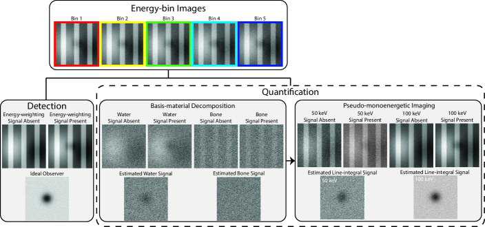
Figure 1: An illustration of detection and quantification of a known water signal in a known water-and-bone background. For detection, the ideal observer applies a spatio-energetic signal template. For quantification, the image is decomposed into water and bone basis materials, which can be used to produce pseudo-monoenergetic images.

Similar to Persson et al,¹³; ¹⁵; ¹⁷ we define an ideal SXD as one that does not blur the incident distribution of x-ray quanta in the spatial domain, does not distort the spectrum of photon energies incident upon it, does not increase the noise inherent in the incident x-ray quanta, and has an infinite number of infinitesimal energy bins.

With this definition, in the background region of an image, the average number of detected photons ($\bar{c}$) per unit energy per unit area is given by

$$\dfrac{\partial^{2}\bar{c}_{\mathrm{ideal}}}{\partial E\partial A}=\phi\left(E\right)$$ (3)

where $\phi\left(E\right)$ [keV^-1cm^-2] represents the fluence per unit energy incident upon the SXD. In what follows, we assume that $\phi\left(E\right)$ does not vary with position when the signal to be detected or quantified is absent. The corresponding NPS per unit energy per unit area is given by

$$\dfrac{\partial^{2}W_{c,\mathrm{ideal}}}{\partial E\partial A}=\phi\left(E\right).$$ (4)

In what follows, we use these simple definitions to establish the NPS of ideal SXDs for quantification and detection tasks.

II.2 Basis-material Decomposition and Quantification Tasks

The goal of basis material decomposition is to use the spectral information provided by an SXD to decompose the line-integral of x-ray attenuation into two or more basis-material images, as illustrated in Fig. 1. We consider the task of estimating the signal difference due to a perturbation ($\Delta a$) in the area density ($a$) [g/cm²] of one or more basis materials. This task is illustrated in Fig. 1 for a non-uniform (but known) background. Unlike the task in Fig. 1, which has a non-stationary background, we assume the background is uniform and stationary. In this case, the average x-ray fluence per unit energy is uniform over the detector when the signal is absent, but there will be stochastic fluctuations from one region to another.

In the Fourier domain, the average difference in the line integral of x-ray attenuation between signal-present and signal-absent conditions is given by

$$\widehat{\Delta l}\left(\mathbf{u}\right)=\sum_{b=1}^{B}\tfrac{\mu}{\rho}_{b}\left(E\right)\widehat{\Delta a}_{b}\left(\mathbf{u}\right)$$ (5)

where $\widehat{\Delta a}_{b}(\mathbf{u})$ [g] represents the Fourier transform of the signal difference of basis material $b$, $\mu/\rho$ [cm²/g] represents the mass attenuation coefficient, and $B$ represents the number of basis materials. At this point we keep our derivation generic to any number of basis materials. We focus on particular sets of basis materials in Sec. II.4.

The average signal differences ($\widehat{\Delta a}_{b}(\mathbf{u})$) are estimated from noisy SXD data. We can therefore define an NPS for each basis material image in addition to a cross NPS that quantifies noise correlations between basis materials, as described below.

II.2.1 Basis-material NPS for the Ideal SXD

To derive a closed-form expression for the NPS of an ideal SXD, we make the following assumptions about the elements of the vector $\widehat{\Delta\mathbf{a}}$: (1) they are real and (2) their power is concentrated within the Nyquist region defined by the pixel pitch of the detector. The first assumption simplifies our mathematical analysis and the corresponding notation without affecting the mathematical results, which are ultimately independent of $\widehat{\Delta\mathbf{a}}$. The second assumption ensures that aliasing is negligible, which is satisfied when the signal to be detected is larger than a few detector elements in both directions, is common in the field and enables utilizing linear systems theory.

Similar to Rajhabandary et al.¹⁶ and Persson et al.,¹³; ¹⁷ we are interested in establishing an upper limit of image quality. To this end, we assume that $\widehat{\Delta\mathbf{a}}$ is estimated using an unbiased estimator that achieves the Cramer-Rao lower bound. We therefore assume the generalized least squares (GLS) estimator to the linearized basis material problem, which, with the assumptions listed above, can be posed as

$$\widehat{\Delta\mathbf{L}}=\widehat{\mathbf{M}}\widehat{\Delta\mathbf{a}}+\widehat{\boldsymbol{\varepsilon}}$$ (6)

where $\widehat{\boldsymbol{\varepsilon}}$ represents measurement noise which is assumed to be additive, and

$$\widehat{\Delta L}_{i}=-FT\left[\log\dfrac{c_{i,0}+\Delta c_{i}}{\bar{c}_{i,0}}\right]\approx-\dfrac{\widehat{\Delta c}_{i}}{\bar{c}_{i,0}}$$ (7)

where $\widehat{\Delta c}_{i}$ represents the signal difference in energy bin $i$ due to the deviation $\widehat{\Delta\mathbf{a}}$ and $\bar{c}_{i,0}$ is the average number of photons per element in the background region of the image formed from energy bin $i$. The matrix $\widehat{\mathbf{M}}$ is a transformation matrix that maps from the space of log-normalised energy bins to the space of basis materials. In general, $\widehat{\mathbf{M}}$ is frequency dependent, accounting for the spatial resolution of each energy bin in addition to spectral distortions that lead to photons counted in the wrong energy bin. For an ideal detector, the MTF of each energy bin is unity for all spatial frequencies and every incident photon is counted in the correct energy bin. When the linear approximation in Eq. (6) is satisfied, and for a detector with finite energy bins but otherwise ideal, an unbiased estimate is obtained when the matrix $\widehat{\mathbf{M}}$ has elements given by

$$\widehat{M}_{i,b}=\dfrac{{\displaystyle\int_{E_{i}}^{E_{i}+\Delta E_{i}}\tfrac{\mu}{\rho}_{b}\left(E\right)\phi\left(E\right)\mathrm{d}E}}{{\displaystyle\int_{E_{i}}^{E_{i}+\Delta E_{i}}\phi\left(E\right)\mathrm{d}E}}$$ (8)

where $E_{i}$ and $E_{i}+\Delta E_{i}$ [keV] represent the lower and upper limits of energy bin $i$, and (as described above) $\phi\left(E\right)$ [cm^-2keV^-1] represents the fluence per unit energy.

For the GLS estimator, the frequency-dependent covariance matrix of the estimate of $\widehat{\Delta\mathbf{a}}$ is given by

$$\mathbf{W}_{\mathbf{a}}=\left(\widehat{\mathbf{M}}^{T}\mathbf{W}_{L}^{-1}\widehat{\mathbf{M}}\right)^{-1}$$ (9)

where $\mathbf{W}_{L}$ represents the covariance matrix of the measurements $\widehat{\Delta\mathbf{L}}$ when the signal is absent. The $i^{\mathrm{th}}$ diagonal element of $\mathbf{W}_{L}$ represents the NPS of $\Delta L_{i}$; element $i,j$ of $\mathbf{W}_{L}$ represents the cross NPS between $\Delta L_{i}$ and $\Delta L_{j}$ under signal-absent conditions. In all cases, for both ideal and non-ideal detectors, we assume that $\mathbf{W}_{L}$ is real-valued and symmetric, which makes it Hermitian. These assumptions are likely satisfied in real SXDs in which physical processes that result in correlated noise are isotropic in the detector plane, resulting in spatial correlations that are symmetric to reflections about the two axes that define the detector plane.

Combining Eqs. (3), (4) and (7) for a detector with energy bins of finite width but otherwise ideal, the elements of $\mathbf{W}_{L}$ are given by

$$\left[\mathbf{W}_{L}\right]_{i,j}=\delta_{ij}\left(\int_{E_{i}}^{E_{i}+\Delta E_{i}}\phi\left(E\right)\mathrm{d}E\right)^{-1}\,\,\,\text{finite bin widths}$$ (10)

where $\delta_{ij}$ represents the Kronecker delta function.

In the limit of an infinite number of energy bins of infinitesimal width, Eqs. (8) and (10) become

$$M_{i,b}\approx\dfrac{\mu}{\rho}_{b}\left(E_{i}\right)$$ (11)

and

$$\left[\mathbf{W}_{L}\right]_{i,j}\approx\dfrac{\delta_{ij}}{\phi\left(E_{i}\right)\Delta E_{i}}.$$ (12)

Combining these results with Eq. (9) yields

$$\lim_{\Delta E\rightarrow 0}\left[\mathbf{W}_{\mathbf{a}}^{-1}\right]_{b,b^{\prime}} =\bar{q}\left\langle\tfrac{\mu}{\rho}_{b},\tfrac{\mu}{\rho}_{b^{\prime}}\right\rangle_{\phi}$$ (13)

where $\bar{q}=\int_{0}^{\infty}\phi(E)\mathrm{d}E$ and $\left\langle(\mu/\rho)_{b},\right.\left.(\mu/\rho)_{b^{\prime}}\right\rangle_{\phi}$ represents the inner product of $(\mu/\rho)_{b}$ and $(\mu/\rho)_{b^{\prime}}$ with respect to $\phi(E)/\bar{q}$:

$$\left\langle\tfrac{\mu}{\rho}_{b},\tfrac{\mu}{\rho}_{b^{\prime}}\right\rangle_{\phi}=\dfrac{1}{\bar{q}}{\displaystyle\int_{0}^{\infty}\tfrac{\mu}{\rho}_{b}\left(E\right)\tfrac{\mu}{\rho}_{b^{\prime}}\left(E\right)\phi\left(E\right)\mathrm{d}E}.$$ (14)

We therefore have

$$\mathbf{W}_{\mathbf{a},\mathrm{ideal}}=\dfrac{1}{\bar{q}}\mathbf{M}_{2}^{-1}$$ (15)

where element $b,b^{\prime}$ of the matrix $\mathbf{M}_{2}$ is given by Eq. (14) and $\mathbf{W}_{\mathbf{a},\mathrm{ideal}}$ represents the frequency-dependent covariance matrix of basis materials for the ideal detector defined in Sec. II.1. The matrix $\mathbf{M}_{2}$ has units of cm⁴/g² and the fluence has units of cm^-2 which yields units of g²/cm² for the elements of $\mathbf{W}_{\mathbf{a},\mathrm{ideal}}$, as necessary. The $b^{\mathrm{th}}$ diagonal element of $\mathbf{W}_{\mathbf{a},\mathrm{ideal}}$ represents the NPS of basis material $b$; element $b,b^{\prime}$ the cross NPS between basis materials $b$ and $b^{\prime}$. The cross NPS between materials $b$ and $b^{\prime}$ is in general non-zero for an ideal SXD because the mass attenuation coefficients of any two basis materials do not form an orthogonal basis set with respect to the x-ray spectrum $\phi_{0}(E)$, i.e. the right side of Eq. (14) is non-zero for $b\neq b^{\prime}$. For example, the product of the mass attenuation coefficients of Al, poly-methyl-methacrylate (PMMA) and iodine, which are common basis materials, are shown in Fig. 2.

Equation (15) is a novel theoretical contribution of this work. It is useful because the matrix $\mathbf{M}_{2}$ (or its inverse) can be tabulated for standardized x-ray spectra for basis sets of relevance, as described in Sec. II.4.

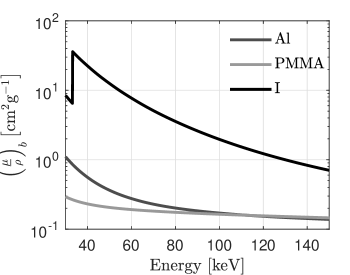
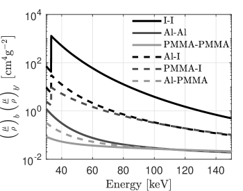
Figure 2: The top plot shows the mass-attenuation coefficients of Al, PMMA and Iodine. The bottom plot shows the products of mass-attenuation coefficients, which are relevant for the inner product in Eq. (14).

II.2.2 DQE for Quantification Tasks

For an ideal detector, the frequency-dependent squared SNR of the unbiased GLS estimate of the area density of basis material $b$ is given by

$$\mathrm{SNR}_{b,\mathrm{ideal}}^{2}=\dfrac{\widehat{\Delta a}_{b}^{2}}{\left[\mathbf{W}_{\mathbf{a},\mathrm{ideal}}\right]_{b,b}}.$$ (16)

If we similarily assume an unbiased GLS estimate for a non-ideal detector, the resulting SNR given is by

$$\mathrm{SNR}_{b}^{2}=\dfrac{\widehat{\Delta a}_{b}^{2}}{\left[\mathbf{W}_{\mathbf{a}}\right]_{b,b}}$$ (17)

where $\mathbf{W}_{\mathbf{a}}$ is the non-ideal counterpart to $\mathbf{W}_{\mathbf{a},\mathrm{ideal}}$, and is given by Eq. (9) with $\widehat{\mathbf{M}}$ given by

$$\widehat{M}_{i,b}=\dfrac{{\displaystyle\int_{0}^{\infty}\tfrac{\mu}{\rho}_{b}\left(E\right)\phi\left(E\right)T_{i}\left(\mathbf{u},E\right)\mathrm{d}E}}{{\displaystyle\int_{0}^{\infty}\phi\left(E\right)T_{i}\left(0,E\right)\mathrm{d}E}}\,\,\,\mathrm{non\,ideal}$$ (18)

where $T_{i}(\mathbf{u},E)$ [cm²] represents the energy-dependent characteristic transfer function of energy bin $i$. The characteristic transfer function is the Fourier transform of the impulse response function.²² The impulse response function of energy bin $i$ of an SXD is equal to the number of photons detected in energy bin $i$ of a detector element centered at position $\mathbf{r}$ given a photon incident at the origin.²⁵ In writing Eq. (18) we have assumed that $T_{i}(\mathbf{u},E)$ is real, which is satisfied if the impulse response function of each energy bin is real and symmetric. Element $i,b$ of $\widehat{\mathbf{M}}$ represents the frequency-dependent response of energy $i$ to the spectrum $\phi$ weighted by the mass-attenuation coefficient of basis material $b$. It could be measured using thin filters comprised of the individual basis materials and a slanted edge.

Taking the ratio of Eq. (17) to Eq. (16) yields the DQE for quantification tasks:

$$\mathrm{DQE}_{b}^{Q}\left(\mathbf{u}\right)=\dfrac{\left[\mathbf{M}_{2}^{-1}\right]_{b,b}}{\bar{q}\left[\left(\widehat{\mathbf{M}}^{T}\mathbf{W}_{L}^{-1}\widehat{\mathbf{M}}\right)^{-1}\right]_{b,b}}$$ (19)

where the superscript $Q$ indicates that the task is quantification. This result shows that knowledge of $\mathbf{M}_{2}^{-1}$ is required to compute the DQE for quantification tasks. We provide tables of the elements of $\mathbf{M}_{2}^{-1}$ for selected tasks and standardized spectra, as described in Sec. II.4.

II.2.3 Pseudo-monoenergetic Imaging

One purpose of basis material decomposition is to produce pseudo monoenergetic images by estimating the energy-dependent line-integral of x-ray attenuation in Eq. (5). Assuming an unbiased GLS estimate of $\widehat{\Delta\mathbf{a}}$ and ideal detectors with an infinite number of infinitesimal energy bins, the noise power of a pseudo monoenergetic image is given by

$$W_{l,\mathrm{ideal}}=\dfrac{1}{\bar{q}}\bm{\mu}^{T}\mathbf{M}_{2}^{-1}\bm{\mu}$$ (20)

where $\bm{\mu}$ represents a vector of basis material mass attenuation coefficients. Note that although not explicit, $W_{l,\mathrm{ideal}}$ is a function of energy through $\boldsymbol{\mu}$, the elements of which represent the energy-dependent mass-attenuation coefficients of basis materials.

Similar to the basis material SNR, we can normalize the SNR of the unbiased GLS estimate of $\widehat{\Delta l}$ for non-ideal detectors by that of ideal detectors to provide a DQE:

$$\mathrm{DQE}^{E}\left(\mathbf{u}\right)=\dfrac{1}{\bar{q}}\dfrac{\bm{\mu}^{T}\mathbf{M}_{2}^{-1}\bm{\mu}}{\bm{\mu}^{T}\left(\widehat{\mathbf{M}}^{T}\mathbf{W}_{L}^{-1}\widehat{\mathbf{M}}\right)^{-1}\bm{\mu}}$$ (21)

where $(\widehat{\mathbf{M}}^{T}\mathbf{W}_{L}^{-1}\widehat{\mathbf{M}})^{-1}=\mathbf{W}_{a}$ represents the basis material noise power matrix for non-ideal detectors and the superscript $E$ indicates mono-energetic imaging. This ratio is equivalent to the definition of the DQE for pseudo-monoenergetic tasks described by Rahjabandary et al.¹⁶ Again, providing a normalized metric of image quality requires knowledge of $\mathbf{M}_{2}^{-1}$.

II.3 Detection Tasks

In a detection task, the ideal observer uses their knowledge of the signal and noise properties of the energy-bin images to whiten the image data by decorrelating it in the spatial and energy domains and then applying the signal template to the data.²⁶; ¹³ In the energy domain, applying the signal template takes the form of energy weighting;²⁷; ¹³ in the spatial domain, the known shape of the signal is used as a window through which the image is viewed, as illustrated in Fig. 1. For an SXD, the squared SNR of the ideal-observer is given by¹³; ¹⁵

$$\mathrm{SNR}^{2}=\int_{\mathrm{Nyq}}\widehat{\Delta\boldsymbol{\mathrm{c}}}^{T}\mathbf{W}^{-1}\widehat{\Delta\boldsymbol{\mathrm{c}}}\mathrm{d}\mathbf{u}$$ (22)

where $\widehat{\Delta\boldsymbol{\mathrm{c}}}$ [cm²] represents a vector with elements equal to the signal difference of each energy bin:

$$\widehat{\Delta c}_{i}\left(\mathbf{u}\right)=\int_{0}^{\infty}T_{i}\left(\mathbf{u},E\right)\widehat{\Delta\Phi}\left(\mathbf{u},E\right)\mathrm{d}E$$ (23)

where, for small perturbations, $\Delta\Phi\left(\mathbf{u},E\right)$ [keV^-1] is given by

$$\widehat{\Delta\Phi}\left(\mathbf{u},E\right)=\phi\left(E\right)\sum_{b=1}^{B}\tfrac{\mu}{\rho}_{b}\left(E\right)\widehat{\Delta a}_{b}.$$ (24)

For a detector with energy bins of finite width but otherwise ideal, $\Delta S_{i}\left(\mathbf{u}\right)$ becomes

$$\widehat{\Delta c}_{i}\left(\mathbf{u}\right)=\bar{c}_{i,0}\sum_{b=1}^{B}\widehat{M}_{i,b}\widehat{\Delta a}_{b}$$

where $\widehat{M}_{i,b}$ is given by Eq. (8). We also note that $W_{ij}=\delta_{ij}\bar{c}_{i}A$ for a detector with energy bins of finite width but otherwise ideal. The ideal-observer SNR then becomes

$$\mathrm{SNR}^{2}=\int\sum_{b=1}^{B}\sum_{b^{\prime}=1}^{B}\sum_{i=1}^{N}\bar{c}_{i,0}\tfrac{\mu}{\rho}_{i,b}\tfrac{\mu}{\rho}_{i,b^{\prime}}\widehat{\Delta a}_{b}\widehat{\Delta a}_{b^{\prime}}\mathrm{d}\mathbf{u}.$$ (25)

In the limit of an infinite number of infinitesimal energy bins

$$\mathrm{SNR}_{\mathrm{ideal}}^{2}=\bar{q}\int\widehat{\Delta\mathbf{a}}^{T}\mathbf{M}_{2}\widehat{\Delta\mathbf{a}}\,\mathrm{d}\mathbf{u}$$ (26)

where the elements of $\mathbf{M}_{2}$ are given by Eq. (14). We can alternatively express the SNR in terms of $\mathbf{W}_{\mathbf{a},\mathrm{ideal}}$ by making use of Eq. (15):

$$\mathrm{SNR}_{\mathrm{ideal}}^{2}=\int\widehat{\Delta\mathbf{a}}^{T}\mathbf{W}_{\mathbf{a},\mathrm{ideal}}^{-1}\widehat{\Delta\mathbf{a}}\,\mathrm{d}\mathbf{u}.$$ (27)

Equations (26) and (27) show that the ideal observer SNR for ideal detectors is determined by the matrix of basis material noise power for the ideal detector, which is in turn determined by the matrix of inner products $\mathbf{M}_{2}$.

II.3.1 DQE for Single-material Detection Tasks

We consider the case when the signal difference is due to the perturbation of a single basis material. In this case, the ideal ideal-observer SNR is given by

$$\mathrm{SNR}_{\mathrm{ideal},b}^{2}=\int\widehat{\Delta a_{b}}^{2}\left[\mathbf{W}_{\mathbf{a},\mathrm{ideal}}^{-1}\right]_{b,b}\,\mathrm{d}\mathbf{u}.$$ (28)

The non-ideal ideal-observer SNR can be shown to be given by

$$\mathrm{SNR}_{b}^{2} =\int_{\mathrm{Nyq}}\widehat{\Delta a}_{b}^{2}\,\widehat{\boldsymbol{\mathrm{M}}}_{b}^{T}\mathbf{W}_{L}^{-1}\widehat{\boldsymbol{\mathrm{M}}}_{b}\mathrm{d}\mathbf{u}$$ (29)

where $\widehat{\mathbf{M}}_{b}$ represents column $b$ of the matrix with elements given by Eq. (18). In writing Eq. (29) we have changed the basis set from that of energy bin counts to that of the basis materials. The integrands of Eqs. (28) and (29) represent frequency-dependent SNRs; dividing the latter by the former yields the DQE of basis material $b$ for detection tasks:

$$\mathrm{DQE}_{b}^{D}\left(\mathbf{u}\right)=\dfrac{\widehat{\boldsymbol{\mathrm{M}}}_{b}^{T}\mathbf{W}_{L}^{-1}\widehat{\boldsymbol{\mathrm{M}}}_{b}}{\bar{q}\left[\mathbf{M_{2}}\right]_{b,b}}$$ (30)

where the superscript $D$ indicates “detection.” Again, we see that computing the frequency-dependent DQE requires knowledge of the matrix $\mathbf{M}_{2}$.

II.4 Calculation of $\mathbf{W}_{\mathbf{a},\mathrm{ideal}}$

We calculated the matrix of inner products ($\mathbf{M}_{2}$) and its inverse for RQA x-ray spectra (listed in Tab. 1) and selected sets of basis materials, as described below.

II.4.1 X-ray Spectrum

We simulated poly-energetic x-ray spectra using the Tucker and Barnes algorithm²⁸ implemented using an in-house MATLAB script. We simulated a tungsten (W) anode, a target angle of 10 degrees and inherent filtration by 2.38 mm of pyrex, 2.66 mm of Lexan, 3.06 mm of oil and 1.5 mm of Al. We simulated the number of photons in 0.1-keV energy bins for energies ranging from 20 keV to the maximum energy of the x-ray spectrum. We then used the Lambert-Beer Law to simulate hardening of x-ray spectra by the additional Al filtration listed in Tab. 1. The HVL was then verified by comparing the HVLs of the modeled spectra with the desired HVLs in Tab. 1. The thickness of the added Al filtration was increased or decreased until the modeled HVL was within 0.25% of the desired HVL. For the HVL verification, we calculated the air Kerma using the mass energy transfer coefficient of air in the NIST database.

II.4.2 Basis Materials

The elements of the matrix $\mathbf{M}_{2}$ are functions of the mass attenuation coefficients of the set of basis materials. Clinically relevant basis materials include soft-tissue and bone, in addition to contrast agents such as iodine and gadolinium. Because of their similar mass attenuation coefficients, water or PMMA, i.e. acrylic, are often used in place of soft-tissue in x-ray imaging experiments; Al is often used in place of bone. We therefore computed $\mathbf{M}_{2}$ for a basis set consisting of PMMA and Al, which are most amenable to experimentation. To accommodate contrast-enhanced imaging, we also computed $\mathbf{M}_{2}$ for basis sets consisting of PMMA, Al and either iodine (I) or gadolinium (Gd).

The mass attenuation coefficients of basis materials were combined with the x-ray spectra described in the preceding section to compute the inner product in Eq. (13). A Riemann sum with 0.1-keV energy bins was used to numerically compute the integral over the energy domain.

II.4.3 Normalization of $\mathbf{W}_{\mathbf{a},\text{ideal}}$

The spectra and basis materials from the preceding section were used to compute $\mathbf{M}_{2}^{-1}$. To be consistent with the IEC, we normalized $\mathbf{M}_{2}^{-1}$ such that it can be converted to the ideal NPS for a given fluence using a measurement of the air Kerma which, unlike the fluence, is directly accessible experimentally. To this end, $\mathbf{W}_{\mathbf{a},\text{ideal}}$ can be expressed as

$$\mathbf{W}_{\mathbf{a},\text{ideal}}=\dfrac{1}{K_{a}}\left(\dfrac{\partial K_{a}}{\partial q}\mathbf{M}_{2}^{-1}\right)$$ (31)

where $K_{a}$ [$\mu$Gy] and $\partial K_{a}/\partial q$ [$\mu$Gy cm²] represent the air Kerma and the air Kerma per unit fluence, respectively. We tabulated the term in parenthesis in Eq. (31) in units of g²cm^-2$\mu$Gy. In practice, calculating $\mathbf{W}_{\mathbf{a},\text{ideal}}$ would be achieved by dividing the tabulated values of $(\partial K_{a}/\partial q)\mathbf{M}_{2}^{-1}$ by the air Kerma used to measure the actual NPS of the SXD under study. We present some example calculations of $(\partial K_{a}/\partial q)\mathbf{M}_{2}^{-1}$ in the results section; tables of $(\partial K_{a}/\partial q)\mathbf{M}_{2}^{-1}$ values for the RQA spectra and basis sets described above are given in the Appendix.

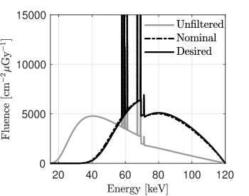
Figure 3: Models of the x-ray spectra used in this work. The nominal and desired spectra are those hardened using the nominal added Al thickness and that which yields a HVL within 0.25% of the HVL prescribed by the IEC.

Equation (31) is useful for normalizing $\mathbf{M}_{2}^{-1}$ for calculation of the DQE, for which the fluence incident on the detector is relevant and obtained from a measurement of air Kerma and tabulated values of $\partial K_{a}/\partial q$. As will be shown in the Results, the resulting noise power for a fixed air Kerma incident on the detector increases with tube voltage, apparently suggesting that lower tube voltages are advantageous. This is somewhat non-intuitive because the fraction of photons transmitted through a patient increases with increasing tube voltage, resulting in more photons reaching the detector for a given patient dose, potentially leading to lower noise per unit patient dose for higher-energy spectra. As such, for the purpose of illustration, we also normalized $\mathbf{M}_{2}^{-1}$ by the air Kerma incident on the patient, which we approximated as a 20-cm-thick water slab. To this end, $\mathbf{W}_{\mathbf{a},\text{ideal}}$ was expressed as

$$\mathbf{W}_{\mathbf{a},\text{ideal}}=\dfrac{1}{K_{a,\mathrm{entrance}}}\left(\dfrac{\partial K_{a,\mathrm{entrance}}}{\partial q}\mathbf{M}_{2}^{-1}\right)$$ (32)

where $K_{a,\mathrm{entrance}}$ [$\mu$Gy] and $\partial K_{a,\mathrm{entrance}}/\partial q$ [$\mu$Gy cm²] represent the air Kerma incident on the patient and the entrance air Kerma per unit fluence incident on the detector, respectively.

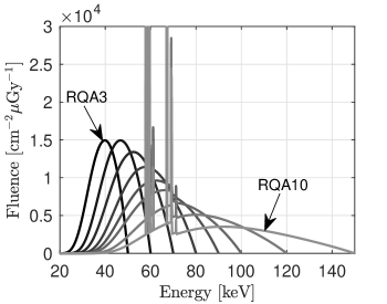
Figure 4: X-ray spectra used to calculate the NPS of ideal SXDs.

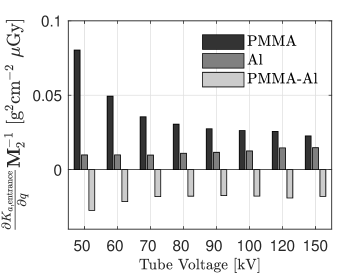
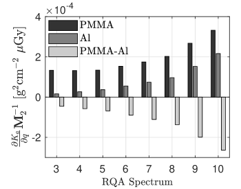
Figure 5: Bar plots of the noise power of basis-material images of ideal SXDs for a two-material decomposition with PMMA and Al basis materials. The variables $K_{a,\mathrm{entrance}}$, $K_{a}$ and $q$ represent the entrance air Kerma (i.e. that incident on a patient), the air Kerma incident on the detector and the x-ray fluence incident on the detector respectively.

III Results

III.1 X-ray Spectra

Table 2: Properties of RQA x-ray spectra. The nominal tube voltages, nominal Al filtration, and desired HVLs are those prescribed by the IEC.²⁰ The nominal HVL and fluence per unit air Kerma are those calculated using the nominal tube voltages and nominal Al filtrations for x-ray spectra modeled using the Tucker and Barnes algorithm.²⁸ The actual Al filtrations, HVLs and fluences per unit air Kerma are those used to calculate $(\partial K_{a}/\partial q)\mathbf{M}_{2}^{-1}$.

		Al Filtration [mm]		Al HVL [mm]			$\partial q/\partial K_{a}\times 10^{-2}$ [cm-2$\mu$Gy-1]
Spectrum	Tube Voltage [kV]	Nominal	Actual	Desired	Nominal	Actual	Nominal	Actual
RQA3	50	10.0	10.3	3.80	3.77	3.80	22312	22408
RQA4	60	16.0	16.9	5.40	5.33	5.41	27887	28127
RQA5	70	21.0	21.8	6.80	6.74	6.80	31368	31515
RQA6	80	26.0	27.5	8.20	8.09	8.20	33324	33484
RQA7	90	30.0	31.0	9.20	9.15	9.21	33894	33950
RQA8	100	34.0	34.6	10.1	10.0	10.1	33685	33696
RQA9	120	40.0	42.5	11.6	11.5	11.6	32024	31948
RQA10	150	45.0	48.0	13.3	13.2	13.3	28630	28427

Table 2 summarizes the x-ray spectra used to calculate $\mathbf{M}_{2}$. The nominal tube voltages, nominal Al filtration and desired HVLs are those prescribed by the IEC.²⁰ The nominal HVLs and fluences per unit air Kerma are those calculated using the nominal tube voltages and nominal Al filtration for x-ray spectra modeled using the Tucker and Barnes algorithm.²⁸ Figure 3 shows an example of an unfiltered 120-kV spectrum, a 120-kV spectrum hardened by the nominal Al thickness for an RQA9 spectrum, and the desired RQA9 spectrum.

The actual Al filtration, HVLs and fluences per unit air Kerma are those used to calculate $(\partial K_{a}/\partial q)\mathbf{M}_{2}^{-1}$. In all cases, the Al thickness required to achieve the desired Al HVL was greater than the nominal thickness prescribed by the IEC, indicating that our implementation of the Tucker and Barnes algorithm²⁸ produces spectra slightly softer than those that the IEC used to determine the nominal Al thicknesses in Tab. 1. Also, the fluences per unit air Kerma calculated using the nominal Al thickness and the actual Al thickness exceed those reported by the IEC²¹ by 3% to 5%. The spectra calculated using the parameters in Tab. 2 are shown in Fig. 4.

III.2 Basis-material NPS ($\mathbf{W}_{\mathbf{a},\text{ideal}}$)

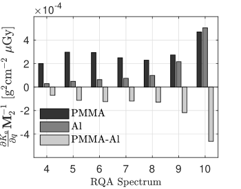
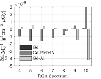
Figure 6: Bar plots of the noise power of basis-material images for ideal SXDs for a three-material decomposition with PMMA, Al and Gd basis materials. The left bar plot shows the NPS for PMMA and Al, in addition to the cross NPS between PMMA and Al. The right bar plot shows the NPS for Gd in addition to the cross NPS between Gd and PMMA and between Gd and Al. Note that the y-scales of the two bar plots are different.

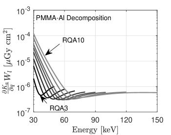
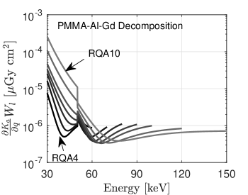
Figure 7: Line-integral noise power normalized by the air Kerma incident upon the detector. The left and right figures correspond to two-material and three-material decompositions, respectively. SNRs for the three-material decomposition are only shown for RQA spectra with maximum energies greater than the K-edge energy of Gd.

Example basis-material noise power spectra (i.e. the elements of $\mathbf{W}_{a}$) are illustrated graphically in Fig. 5 for the two normalizations described in Sec. II.4. Results are shown for a two-material decomposition with a basis set consisting of PMMA and Al. The “PMMA” and “Al” bars represent the noise power in the respective basis material images; the “PMMA-Al” bars represent the cross NPS between PMMA and Al basis materials.

The left bar plot of Fig. 5 shows the inverse of the matrix of inner products ($\mathbf{M}_{2}^{-1}$) normalized by the air Kerma incident on a 20-cm-thick volume of water ($K_{a,\mathrm{entrance}}$) for tube voltages corresponding to the RQA series spectra in the right figure. The left figure shows that, for a fixed entrance Kerma, basis material noise power spectra and cross noise power spectra decrease with increasing tube voltage. This result simply reflects the greater attenuation of low-energy photons, which results in fewer quanta incident on the detector for a fixed entrance Kerma.

The right bar plot shows $\mathbf{M}_{2}^{-1}$ normalized by the air Kerma incident on the detector ($K_{a}$). The results in the right figure are those which are required to normalize the DQE for detection and quantification tasks, including pseudo-monoenergetic imaging. For a fixed detector Kerma, the magnitude of basis-material noise power spectra and cross noise power spectra increases with increasing tube voltage. This is likely because the basis-material mass attenuation coefficients are less distinct from each other at higher energies, resulting in poorer conditioning of $\mathbf{M}_{2}$.

Figure 6 shows bar plots of basis-material noise power spectra for a three-material decomposition with PMMA, Al and Gd basis materials. Results are shown for x-ray spectra with maximum energies greater than the K-edge energy of Gd. The noise power spectra in Fig. 6 are normalized by the air Kerma at the detector. The left bar plot of Fig. 6 shows the NPS for PMMA and Al, in addition to the cross NPS between PMMA and Al. The right bar plot shows the NPS of Gd, in addition to the cross NPS between Gd and PMMA and between Gd and Al.

Comparing the left bar plot of Fig. 6 with the right bar plot of Fig. 5 shows that the addition of Gd to the basis set increases noise in the ideal PMMA and Al basis images. This is expected because the inclusion of a third basis material is an attempt to extract more information from the energy-bin data. Comparing the left and right bar plots of Fig. 6 shows that the noise in the ideal Gd basis image is much lower than that in the PMMA and Al basis images. The Gd cross terms are also much lower than the cross terms between PMMA and Al. These latter two results are likely due to the presence of the Gd K-edge at $\sim$50-keV, which results in a mass-attenuation coefficient with a substantially different energy dependence than that of PMMA and Al.

III.3 Pseudo-monoenergetic NPS ($W_{l,\text{ideal}}$)

Examples of line-integral noise power spectra for ideal SXDs are illustrated graphically in Fig. 7, in which noise power spectra are normalized by the air Kerma incident upon the detector. The x-axis represents the pseudo-energy at which the line integral is evaluated. The left plot of Fig. 7 shows results for a two-material decomposition with PMMA and Al basis materials; the right plot shows results for a three-material decomposition with PMMA, Al and Gd basis materials.

For the two-material decomposition, the different curves (each corresponding to a different spectrum) show similar trends, each having a minimum between 30 keV and the maximum energy of the x-ray spectrum. Although not shown here, the minima occur at energies slightly less than the average energies of the x-ray spectra. For example, the average energies of the RQA7 and RQA9 spectra are 63 keV ant 76 keV, respectively, and the corresponding minima occur at approximately 59 keV and 70 keV, respectively. Similar results are observed for the three-material decomposition, although the presence of the Gd K-edge introduces a discontinuity in the NPS.

IV Discussion

We presented simple, closed-form expressions for the noise power spectra of ideal SXDs for detection and quantification tasks. We showed that a single matrix ($\mathbf{M}_{2}$) determines the NPS of ideal SXDs for detection and quantification, including basis-material decomposition and pseudo-monoenegetic imaging. The inverse of this matrix is proportional (through the x-ray fluence) to the covariance matrix (per unit frequency) of an unbiased GLS estimate of a perturbation ($\Delta\mathbf{a}$) of basis material area densities. We showed that the elements of $\mathbf{M}_{2}$ are given by inner products of the mass-attenuation coefficients with respect to the spectrum of photons incident on the x-ray detector.

The matrix $\mathbf{M}_{2}$ is determined uniquely by the x-ray spectrum incident upon the detector and the basis set, and therefore can be tabulated for standardized x-ray spectra and common basis sets, as was done here. The resulting tables (in Appendix A) can be used to normalize experimental measurements of the frequency-dependent SNR of SXDs for calculation of the task-dependent DQE for detection tasks (Eq. 30) and quantification tasks, including basis-material decomposition (Eq. 19) and pseudo-monoenergetic imaging (Eq. 21). We did not tabulate values of the noise power for pseudo-monoenergetic imaging, but these can easily be obtained by combining the mass-attenuation coefficients of basis materials with the tables in Appendix A.

Whereas the DQE of a conventional, non-energy-resolving x-ray detector is a single number, the DQE of an SXD is dependent on the imaging task, so that it becomes necessary to distinguish between quantification tasks (Eq. (19) for basis images and Eq. (21) for pseudo-monoenergetic images) or a detection task (Eq. (30)). In a detection task, the objective is to determine whether a particular feature is present in the image or not. In the context of spectral x-ray imaging, this means aggregating the available information in all energy bins or, after material decomposition, all basis material images. Even if the signal difference to be detected is limited to one single basis material, the ideal observer will still incorporate data from the other basis material images, accounting for noise correlations between these basis material images in an optimal way. In quantification tasks, on the other hand, the objective is to measure a numerical value as accurately and precisely as possible, e.g. the line integral of one of the basis coefficients or of the attenuation at a particular energy. Of course, it may then be of interest to assess the performance for a detection task in such an estimated image, in which case Equation (19) describes the detection performance relative to an ideal detector when only a single basis image is available as opposed to Eq. (30) which describes detection performance based on all basis images together. Eq. (19) can therefore be relevant for those detection tasks where the other basis images can add confusion, such as when using a K-edge image to detect elevated contrast agent concentrations against a cluttered anatomical background.

Calculating the task-dependent DQEs in Eqs. (19), (21) and (30) requires measurement of the NPS of individual energy bins in addition to the cross NPS between energy bins, for example using the approach described by Tanguay et al.¹⁸ Also required for experimental DQE analysis is the matrix $\widehat{\mathbf{M}}$ with elements given by Eq. (18), which is proportional to the MTF of energy bin $i$ for a spectrum that is weighted by the mass-attenuation coefficient of basis material $b$. For basis sets consisting of PMMA and Al, these elements could be measured using the conventional slanted-edge approach²³ for spectra transmitted through thin PMMA or Al absorbers. The development of such an experimental framework is beyond the scope of this work, but Persson et al.¹³; ¹⁷ modeled the DQE of cadmium telluride and silicon for quantification and detection tasks for computed tomography imaging conditions. Their models predicted that realistic CdTe SXDs produce DQEs $\sim$0.85 for water detection tasks; for quantification tasks, the DQE drops to $\sim$0.35. Development of an experimental framework for task-based DQE analysis is a focus of ongoing research.

We chose to consider PMMA and Al basis materials because these materials are widely available, relatively inexpensive, and convenient for experimentation. While water and bone basis materials may be more clinically relevant, water is cumbersome experimentally, and bone (or bone-equivalent plastic) is not as readily available as Al. The tabulated matrix values can also easily be transformed to another set of basis materials, if the new set approximately lies within the span of the original ones. Specifically, if we let $\left\{\tfrac{\mu}{\rho}_{b^{\prime}}^{\prime}\left(E\right)\right\}_{b^{\prime}=1,\ldots,B}$ denote such a second set of basis materials, related to the original basis materials by a transformation matrix $\mathbf{B}$ according to $\tfrac{\mu}{\rho}_{b^{\prime}}^{\prime}\left(E\right)=\sum_{b}\tfrac{\mu}{\rho}_{b}\left(E\right)B_{bb^{\prime}}$, $\mathbf{M}_{2}$ will be transformed into $\mathbf{M}_{2}^{\prime}=\mathbf{B}^{T}\mathbf{MB}$. This formula can be used to calculate the quantification DQE for light elements other than PMMA and Al, but if another K-edge element is introduced, the elements of $\mathbf{M}_{2}$will have to be recomputed using Eq. (14).

We used RQA spectra for pragmatic reasons as well. Specifically, RQA x-ray spectra are standardized and easily reproducible across different laboratories. Secondly, RQA spectra have been adopted for assessment of the DQE of conventional detectors. In practice, it will likely be unnecessary to report a DQE for all the RQA spectra considered in this work, and the lower-energy spectra may ultimately be irrelevant. The most relevant RQA spectra for SXDs will likely be those produced using tube voltages greater than 100 kV, since higher tube voltages tend to produce better image quality for SXDs.

V Conclusions

The conclusions of this work are:

1. Normalization of the task-dependent DQE of spectroscopic x-ray detectors requires knowledge of a matrix ($\mathbf{M}_{2}$) that is uniquely determined by the x-ray spectrum incident upon the detector and the mass-attenuation coefficients of the basis materials with respect to which the signal to be detected or quantified is decomposed. (See Eq. 14).

2. When divided by the air Kerma ($K_{a}$) incident upon the detector, the diagonal elements of the matrix $(\partial K_{a}/\partial q)\mathbf{M}_{2}^{-1}$ [g²cm^-2$\mu$Gy] (where $q$ [cm^-2] represents fluence) are equal to the noise power spectra of basis-material images produced by an ideal spectroscopic x-ray detector; the off-diagonal elements represent cross noise power spectra between basis materials.

3. Tables 3, 4 and 5 tabulate the elements of $(\partial K_{a}/\partial q)\mathbf{M}_{2}^{-1}$ for RQA x-ray spectra for selected basis sets, and can be incorporated into an experimental framework for DQE analysis of spectroscopic x-ray detectors, similar to the way tabulated values of the SNRs of RQA x-ray fluences (in Tab. 1) are used in conventional DQE analyses.

VI Conflict of Interest Statement

M. Persson discloses past financial interests in Prismatic Sensors AB (now part of GE Healthcare).

Appendix A Noise Power Tables

Tables 3, 4 and 5 list the basis-material noise power spectra and cross noise power spectra for ideal SXDs for PMMA-Al, PMMA-Al-I and PMMA-Al-Gd basis sets.

Table 3: Noise power of an ideal SXD for PMMA-Al decomposition tasks for RQA series x-ray spectra.

	$\partial K_{a}/\partial q\mathbf{M}_{2}^{-1}$ [g2cm-2$\mu$Gy]
Spectrum	PMMA	Al	PMMA-Al
RQA3	1.33$\times$10-4	1.64$\times$10-5	-4.54$\times$10-5
RQA4	1.32$\times$10-4	2.65$\times$10-5	-5.75$\times$10-5
RQA5	1.34$\times$10-4	3.70$\times$10-5	-6.84$\times$10-5
RQA6	1.53$\times$10-4	5.52$\times$10-5	-8.97$\times$10-5
RQA7	1.75$\times$10-4	7.40$\times$10-5	-1.11$\times$10-4
RQA8	2.02$\times$10-4	9.67$\times$10-5	-1.37$\times$10-4
RQA9	2.68$\times$10-4	1.53$\times$10-4	-1.98$\times$10-4
RQA10	3.32$\times$10-4	2.16$\times$10-4	2.63$\times$10-4

Table 4: Noise power of an ideal SXD for PMMA-Al-I decomposition tasks for RQA series x-ray spectra.

	$\partial K_{a}/\partial q\mathbf{M}_{2}^{-1}$ [g2cm-2$\mu$Gy]
Spectrum	PMMA	Al	I	PMMA-Al	PMMA-I	Al-I
RQA3	3.34$\times 10^{-4}$	2.04$\times 10^{-5}$	8.18$\times 10^{-9}$	-7.14$\times 10^{-5}$	-1.18$\times 10^{-6}$	1.80$\times 10^{-7}$
RQA4	1.48$\times 10^{-4}$	3.23$\times 10^{-5}$	1.46$\times 10^{-8}$	-4.78$\times 10^{-5}$	-4.83$\times 10^{-7}$	-2.91$\times 10^{-7}$
RQA5	1.43$\times 10^{-4}$	1.06$\times 10^{-4}$	3.90$\times 10^{-8}$	-9.31$\times 10^{-5}$	5.85$\times 10^{-7}$	-1.64$\times 10^{-6}$
RQA6	3.47$\times 10^{-4}$	4.69$\times 10^{-4}$	1.43$\times 10^{-7}$	-3.73$\times 10^{-4}$	5.25$\times 10^{-6}$	-7.67$\times 10^{-6}$
RQA7	8.98$\times 10^{-4}$	1.32$\times 10^{-3}$	3.63$\times 10^{-7}$	-1.06$\times 10^{-3}$	1.62$\times 10^{-5}$	-2.13$\times 10^{-5}$
RQA8	2.31$\times 10^{-3}$	3.38$\times 10^{-3}$	8.66$\times 10^{-7}$	-2.77$\times 10^{-3}$	4.28$\times 10^{-5}$	-5.33$\times 10^{-5}$
RQA9	1.23$\times 10^{-2}$	1.73$\times 10^{-2}$	3.98$\times 10^{-6}$	-1.46$\times 10^{-2}$	2.19$\times 10^{-4}$	-2.61$\times 10^{-4}$
RQA10	3.60$\times 10^{-2}$	4.86$\times 10^{-2}$	1.05$\times 10^{-5}$	-4.18$\times 10^{-2}$	6.11$\times 10^{-4}$	-7.12$\times 10^{-4}$

Table 5: Noise power of an ideal SXD for PMMA-Al-Gd decomposition tasks for RQA series x-ray spectra.

	$\partial K_{a}/\partial q\mathbf{M}_{2}^{-1}$ [g2cm-2$\mu$Gy]
Spectrum	PMMA	Al	Gd	PMMA-Al	PMMA-Gd	Al-Gd
RQA3	1.67$\times 10^{-3}$	6.64$\times 10^{-3}$	2.83$\times 10^{-5}$	-3.23$\times 10^{-3}$	-2.09$\times 10^{-4}$	4.33$\times 10^{-4}$
RQA4	2.00$\times 10^{-4}$	2.90$\times 10^{-5}$	1.40$\times 10^{-8}$	-7.06$\times 10^{-5}$	-9.81$\times 10^{-7}$	1.88$\times 10^{-7}$
RQA5	2.97$\times 10^{-4}$	4.93$\times 10^{-5}$	1.61$\times 10^{-8}$	-1.13$\times 10^{-4}$	-1.62$\times 10^{-6}$	4.45$\times 10^{-7}$
RQA6	2.94$\times 10^{-4}$	6.36$\times 10^{-5}$	1.88$\times 10^{-8}$	-1.24$\times 10^{-4}$	-1.62$\times 10^{-6}$	3.97$\times 10^{-7}$
RQA7	2.49$\times 10^{-4}$	7.48$\times 10^{-5}$	2.03$\times 10^{-8}$	-1.19$\times 10^{-4}$	-1.23$\times 10^{-6}$	1.30$\times 10^{-7}$
RQA8	2.29$\times 10^{-4}$	9.91$\times 10^{-5}$	2.28$\times 10^{-8}$	-1.29$\times 10^{-4}$	-7.77$\times 10^{-7}$	-2.32$\times 10^{-7}$
RQA9	2.74$\times 10^{-4}$	2.16$\times 10^{-4}$	3.42$\times 10^{-8}$	-2.18$\times 10^{-4}$	4.54$\times 10^{-7}$	-1.47$\times 10^{-6}$
RQA10	4.70$\times 10^{-4}$	5.05$\times 10^{-4}$	6.12$\times 10^{-8}$	-4.63$\times 10^{-4}$	2.91$\times 10^{-6}$	-4.20$\times 10^{-6}$

Appendix B Table of Symbols and Relation to Previous Work

Table 6 lists some of the important quantities used in this work together with the corresponding quantities in Persson et al.¹³

Table 6: Summary of important quantities together with the corresponding quantities in Persson et al.¹³. In the right column, $\rho_{b}$ denotes the density of basis material $b$ and $d_{i}$ denotes the position-independent background counts in bin $i$. Subscript indices are consistent with the present work rather than Persson et al.¹³.

Description	Symbol	Unit	Corresponding notation in 13
Signal difference in frequency domain	$\widehat{\Delta a}_{b}$	g	$\rho_{b}\Delta\tilde{A}_{b}$
Normalized bin counts difference in frequency domain	$\widehat{\Delta L}_{i}$	cm2	$-\Delta D_{i}^{s}\Delta_{x}\Delta_{y}/d_{i}^{s}$
Inner product matrix element	$\left[\mathbf{M}_{2}\right]_{b,b^{\prime}}$	cm4g-2	N/A
Transformation matrix element	$\widehat{M}_{i,b}$	cm2g-1	$-\frac{1}{d_{i}^{s}}\frac{\Delta_{x}\Delta_{y}}{\rho_{b}\overline{q}^{\mathrm{tot}}}\frac{\partial\overline{q}^{\mathrm{tot}}}{\partial A_{b}}H_{i,b}^{\mathcal{B}}$
Incident fluence per unit energy	$\phi$	keV-1cm-2	$\overline{q}$
Incident spectrum difference in frequency domain	$\widehat{\Delta\Phi}$	keV-1	$-\Delta\overline{Q}$
Energy bin counts difference in frequency domain	$\widehat{\Delta c}_{i}$	cm2	$-\Delta\overline{D}_{i}^{s}\Delta_{x}\Delta_{y}$
Transfer function of energy bin	$T_{i}$	cm2	$\Delta_{x}\Delta_{y}H_{i}$
Basis material noise power matrix element	$\left[\mathbf{W}_{\mathbf{a}}\right]_{b,b^{\prime}}$	g2/cm2	$\overline{q}^{\mathrm{tot}}{}^{2}\frac{\left[\left.\mathsf{NEQ}^{\mathcal{B}}\right.^{-1}\right]_{b,b^{\prime}}}{\frac{\partial\overline{q}^{\mathrm{tot}}}{\partial A_{b}}\frac{\partial\overline{q}^{\mathrm{tot}}}{\partial A_{b^{\prime}}}}\rho_{b}\rho_{b^{\prime}}$

References

- (1) M. Lundqvist, B. Cederstrom, V. Chmill, M. Danielsson, and B. Hasegawa, “Evaluation of a photon-counting x-ray imaging system,” IEEE Transactions on Nuclear Science 48, pp. 1530–1536, 2001.
- (2) M. Chmeissani, C. Frojdh, O. Gal, X. Llopart, J. Ludwig, M. Maiorino, E. Manach, G. Mettivier, M. Montesi, C. Ponchut, et al., “First experimental tests with a CdTe photon counting pixel detector hybridized with a medipix2 readout chip,” IEEE Trans. Nuc. Sci. 51(5), pp. 2379–2385, 2004.
- (3) P. M. Shikhaliev, T. Xu, and S. Molloi, “Photon counting computed tomography: Concept and initial results,” Med. Phys. 32, pp. 427–436, Feb 2005.
- (4) E. Roessl and R. Proksa, “K-edge imaging in x-ray computed tomography using multi-bin photon counting detectors,” Phys. Med. Biol. 52, pp. 4679–4696, Aug 2007.
- (5) J. P. Schlomka, E. Roessl, R. Dorscheid, S. Dill, G. Martens, T. Istel, C. Baumer, C. Herrmann, R. Steadman, G. Zeitler, A. Livne, and R. Proksa, “Experimental feasibility of multi-energy photon-counting K-edge imaging in pre-clinical computed tomography,” Phys. Med. Biol. 53, pp. 4031–4047, Aug 2008.
- (6) S. Feuerlein, E. Roessl, R. Proksa, G. Martens, O. Klass, M. Jeltsch, V. Rasche, H.-J. Brambs, M. H. K. Hoffmann, and J.-P. Schlomka, “Multienergy photon-counting K-edge imaging: Potential for improved luminal depiction in vascular imaging,” Radiology 249, pp. 1010–1016, Dec 2008.
- (7) H. Bornefalk, “Task-based weights for photon counting spectral x-ray imaging,” Med. Phys. 38, p. 6065, Nov 2011.
- (8) M. Yveborg, M. Persson, and H. Bornefalk, “Optimal frequency-based weighting for spectral x-ray projection imaging,” IEEE Trans. Med. Imaging. 34(3), pp. 779–787, 2015.
- (9) S. Tao, K. Rajendran, C. H. McCollough, and S. Leng, “Feasibility of multi-contrast imaging on dual-source photon counting detector (PCD) CT: An initial phantom study,” Med. Phys. 46, pp. 4105–4115, 2019.
- (10) D. Richtsmeier, C. A. S. Dunning, K. Iniewski, and M. Bazalova-Carter, “Multi-contrast k-edge imaging on a bench-top photon-counting CT system: Acquisition parameter study,” JINST 15, pp. P10029–P10029, 2020.
- (11) C. A. S. Dunning, J. O’Connell, S. M. Robinson, K. J. Murphy, A. L. Frencken, F. C. J. M. van Veggel, K. Iniewski, and M. Bazalova-Carter, “Photon-counting computed tomography of lanthanide contrast agents with a high-flux 330-m-pitch cadmium zinc telluride detector in a table-top system,” Journal of Medical Imaging 7, p. 1, 2020.
- (12) M. Danielsson, M. Persson, and M. Sjölin, “Photon-counting x-ray detectors for CT,” Phys. Med. Biol. 66(3), p. 03TR01, 2021.
- (13) M. Persson, P. L. Rajbhandary, and N. J. Pelc, “A framework for performance characterization of energy-resolving photon-counting detectors.,” Med. Phys. 45, pp. 4897–4915, Nov. 2018.
- (14) P. L. Rajbhandary, M. Persson, and N. J. Pelc, “Frequency dependent DQE of photon counting detector with spectral degradation and cross-talk,” in Medical Imaging 2018: Physics of Medical Imaging, 10573, p. 1057312, International Society for Optics and Photonics, 2018.
- (15) M. Persson and N. J. Pelc, “Simulation model for evaluating energy-resolving photon-counting CT detectors based on generalized linear-systems framework,” in Medical Imaging 2019: Physics of Medical Imaging, T. G. Schmidt, G.-H. Chen, and H. Bosmans, eds., 10948, pp. 474 – 485, International Society for Optics and Photonics, SPIE.
- (16) P. L. Rajbhandary, M. Persson, and N. J. Pelc, “Detective efficiency of photon counting detectors with spectral degradation and crosstalk,” Med. Phys. 47, pp. 27–36, 2020.
- (17) M. Persson, A. Wang, and N. J. Pelc, “Detective quantum efficiency of photon-counting CdTe and Si detectors for computed tomography: a simulation study,” 7(4), pp. 1 – 28.
- (18) J. Tanguay, D. Richtsmeier, C. Dydula, J. A. Day, K. Iniewski, and M. Bazalova-Carter, “A detective quantum efficiency for spectroscopic x-ray imaging detectors,” Med. Phys. (epub ahead of print), 2021.
- (19) P. L. Rajbhandary, S. S. Hsiehc, and N. J. Pelc, “Effect of spatio-energy correlation in PCD due to charge sharing, scatter, and secondary photons,” in Medical Imaging 2017: Physics of Medical Imaging, pp. 101320V–101320V, International Society for Optics and Photonics, 2017.
- (20) IEC, “Medical diagnostic X-ray equipment - Radiation conditions for use in the determination of characteristics,” International Standard IEC 61267, International Electrotechnical Commission, 2005.
- (21) International Electrotechnical Commission, “IEC 622201: Medical electrical equipment - characteristics of digital x-ray imaging devices. Part 1: Determination of the detective quantum efficiency,” Geneva, Switzerland , 2003.
- (22) I. A. Cunningham, “Applied linear-systems theory,” Handbook of Medical Imaging 1, pp. 79–159, 2000.
- (23) E. Samei, M. J. Flynn, and D. A. Reimann, “A method for measuring the presampled MTF of digital radiographic systems using an edge test device,” Med. Phys. 25, pp. 102–113, Jan 1998.
- (24) J. H. Siewerdsen, I. A. Cunningham, and D. A. Jaffray, “A framework for noise-power spectrum analysis of multidimensional images,” Med. Phys. 29(11), pp. 2655–2671, 2002.
- (25) J. Tanguay and I. A. Cunningham, “Cascaded systems analysis of charge sharing in cadmium telluride photon-counting x-ray detectors,” Med. Phys. 45(5), pp. 1926–1941, 2018.
- (26) H. H. Barrett and K. J. Myers, Image Science: Mathematical and Statistical Foundations, Wiley, 2001.
- (27) M. J. Tapiovaara and R. F. Wagner, “SNR and DQE analysis of broad spectrum x-ray imaging,” Phys. Med. Biol. 30, pp. 519–529, 1985.
- (28) D. M. Tucker, G. T. Barnes, and D. P. Chakraborty, “Semiempirical model for generating tungsten target x-ray spectra,” Med. Phys. 18(2), pp. 211–218, 1991.