The finite-volume thermodynamics of a massive integrable QFT is described in terms of a grand canonical ensemble of loops immersed in a torus and interacting through scattering factors associated with their intersections. The path integral of the loops is evaluated explicitly after decoupling the pairwise interactions by a Hubbard-Stratonovich transformation. The HS fields are holomorphic fields depending on the rapidity and can be expanded in elementary oscillators. The torus partition function is expressed as certain expectation value in the Fock space of these oscillators. In the limit where one of the periods of the torus becomes asymptotically large, the effective field theory becomes mean field type. The mean field describes the infinite-volume thermodynamics which is solved by the Thermodynamical Bethe Ansatz.

1 Introduction

A wide variety of integrable systems in 1+1 dimensions are described in terms of a factorised scattering [1]. The scattering theory provides a very general scheme which applies also for quantum field theories (QFTs) without Lagrangian formulation. Remarkably, the scattering theory, although being defined for asymptotic states in infinite spacetime, can be adjusted to study QFTs with compactified space or time dimensions. It is known since long time [2, 3] that the infinite-volume thermodynamics of a massive QFT can be expressed in terms of its S-matrix only. In 1+1 dimensions, the infinite-volume thermodynamics can be solved exactly by the Thermodynamical Bethe Ansatz (TBA) technique introduced by Yang and Yang [4]. In the early 90’s, Alexey Zamolodchikov [5, 6, 7], showed how to use the TBA to compute exactly the finite-volume ground-state energy at zero temperature. Since then a lot of progress has been made in computing the finite volume/temperature effects in integrable models, including some correlation functions. For a review see e.g [8].

There are reasons to expect that it is possible to formulate also the finite-volume thermodynamics of a massive solvable QFT solely in terms of its scattering data. Indeed, the energies of the excited states in finite volume can be determined, at least in principle, by analytical continuation of the TBA solution [9] which in turn is determined by the S-matrix. Once the full spectrum of the finite-volume Hamiltonian is known, the partition function of the Euclidean QFT on the torus is known as well.

On the other hand, the diagonalisation of the finite-volume Hamiltonian seems, at least at present, to be an extremely difficult task. The only known partition functions of massive theories on the torus are those of the so called generalised free theories characterised by constant S-matrices [15, 16].

In this paper, I propose an alternative formulation of the finite-size thermodynamics, for which no knowledge of the finite-volume energy spectrum is necessary. The formulation in question concerns the simplest case of a theory of one single neutral particle and without bound states in the spectrum. The principal claim is that in a theory with factorised scattering, the torus partition function can be mapped onto the grand canonical ensemble of relativistic loops embedded in the torus and interacting through scattering factors associated with the crossings. In the loop gas description, the finite-volume effects are due to non-contractible loops winding around the time and space cycles.

The advantage of the loop-gas formulation is that one can accomplish a separation, in the spirit of [3], of the dynamical part, which is expressed in terms of the S-matrix, from the statistical part, which appears through the path integral for the loops. This is achieved by performing a Hubbard-Stratonovich type transformation in order to decouple the two-body interaction of the loops. The HS auxiliary fields are associated with the two homology cycles of the torus. The decoupling makes possible to perform explicitly the integration over the loops, including the sum over the winding numbers. The sum over the loops results in an effective interaction potential for the HS fields. In order to generate the Gaudin measure, an extra pair of Faddeev-Popov ghost fields is added.

As a result, the torus partition function is expressed as certain expectation value in an effective quantum field theory (EFT) for a pair of bosonic and fermionic oscillators defined in the complex rapidity plane, with two-point function determined by the S-matrix. In the limit when one of the periods of the torus becomes asymptotically large, this EFT was formulated in [20].

The text is organised as follows. In section 2, the partition function of the QFT on a cylinder is formulated as a loop gas. The aim of this section is to verify that the free energy of the loop gas matches the finite-volume vacuum energy computed by the TBA. First I recall the path integral over loops winding given number of times around the cylinder. Importantly, the path integral in question can be expressed in terms of the wave functions of on-shell particles propagating in the infinite Minkowskian spacetime. The free energy of the loop gas, obtained by summing over all winding numbers, is shown to reproduce correctly the effective central charges of the massive boson and the massive Majorana fermion. Then the same derivation is carried out for a theory with non-trivial scattering with the help of HS transformation. The outcome is the EFT formulated in [20], which has been shown to be equivalent to the TBA.

In section 3, the torus partition functions of the generalised free theories, the free massive boson (FB) and the Ising Field Theory (IFT), are formulated as ensembles of loops immersed in the torus. While the partition function of the free boson is the exponential of the path integral for one loop, this is not the case for the IFT, because the loops interact through minus signs associated with their crossings. Although this is aside of the main goal of this paper, in order to achieve maximal clarity I give a combinatorial derivation of the expression of the modular invariant partition function as a sum of four building blocks found by Itzykson and Saleur [15] and Klassen and Melzer [16], based on the loop gas. Finally, in section 4 I formulate the main result of this paper, the effective field theory for a massive integrable QFT on a torus, with the sinh-Gordon model as an example. The Feynman graph expansion for the EFT is formulated in appendix A.

2 Integrable QFT on an infinite cylinder

In this section, the mapping of the integrable QFT to a loop gas will be studied in detail for the simpler and well studied limit of the $L\times R$ torus in which the $R$-cycle is taken asymptotically large, i.e. when all exponential corrections in $R$ are neglected. This limit describes a QFT in infinite space at finite temperature $\sim 1/L$, with IR cutoff introduced by imposing periodic boundary conditions at distance $R$. In the Hamiltonian formulation with the time direction along the $L$-circle, the partition function reads

$${\mathcal{Z}}^{(L)}={\rm Tr}_{{}_{\!R}}\ e^{-L{\cal H}}$$ (2.1)

where ${\cal H}$ is the infinite-volume Hamiltonian and ${\rm Tr}_{{}_{R}}$ is the trace in the Hilbert space associated with the large space circle $R$. On the other hand, if the space is associated with the $L$-circle, the partition function (2.1) determines the finite-volume vacuum energy

$${\cal E}(L)=-\lim_{R\to\infty}{\log{\mathcal{Z}}^{(L)}\over R}.$$ (2.2)

The aim of this section is to express the finite-volume vacuum energy ${\cal E}(L)$ as the free energy in a statistical ensemble loops embedded in the cylinder. In a free theory, the vacuum energy (2.2) is given by the path integral of a single loop. In a theory with non-trivial factorised scattering, the loops experience pairwise interaction. In this case the free energy of the loop gas is obtained by summing up the cumulant expansion, which is another way to derive the TBA equations.

2.1 Path integral for a loop on a cylinder

In order to develop the loop-gas formalism, let us work out the path integral for a single loop. The path integral $\mathcal{F}^{(L)}$ for a loop immersed in the cylinder is a sum over topological sectors characterised by the number $w$ of times the loop coils around the cylinder,

$$\mathcal{F}^{(L)}=\sum_{w\in\mathbb{Z}}[\mathcal{F}^{(L)}]_{w}.$$ (2.3)

The winding number can take both positive and negative values depending on the orientation and two winding numbers add algebraically.

Let me sketch of the computation of $[\mathcal{F}^{(L)}]_{w}$. For that I will use the obvious relation between the integration measure for loops on the cylinder having given winding number and that the loops in the infinite Euclidean spacetime with inserted discontinuity, as illustrated in fig. 1,

Consider the path integral (per unit volume) for a loop fluctuating in the infinite Euclidean space, with inserted discontinuity $\delta\vec{x}=\{\delta x_{1},\delta x_{2}\}$. Denote this path integral by $\mathcal{F}(\delta\vec{x})$. The path integral in the sector with winding number $w$ is obtained by choosing $\delta x_{1}=0$ and $\delta x_{2}=wL$,

$$[\mathcal{F}^{(L)}]_{w}=RL\ \mathcal{F}(\delta\vec{x})\Big{|}_{\delta\vec{x}=\{0,wL\}}\,.$$ (2.4)

A derivation of the path integral measure for open relativistic loops in infinite Euclidean space is given, for example, in Polyakov’s book [21]. With small adjustments, the derivation there can be applied for closed loops as well. It is however simpler to manipulate the expression for the propagator of a massive scalar relativistic particle in two-dimensional Euclidean (infinite) spacetime

$$\begin{aligned} {\cal G}(\delta\vec{x})&=\int{d^{2}k\over(2\pi)^{2}}\ {e^{i\vec{k}\cdot\delta\vec{x}}\over\vec{k}^{2}+m^{2}}=\int{d^{2}k\over(2\pi)^{2}}\int^{\infty}{d\tau}e^{-(\vec{k}^{2}+m^{2})\tau+i\vec{k}\cdot\delta\vec{x}}.\end{aligned}$$ (2.5)

The integrand in the second representation can be interpreted as the Boltzmann amplitude for loops with a marked point, proper time $\tau$ along the loop, 2-momentum $\vec{k}$, and discontinuity $\vec{x}(\tau)-\vec{x}(0)=\delta\vec{x}$ at the marked point. The integral (2.5) is not yet $\mathcal{F}(\delta\vec{x})$. To obtain $\mathcal{F}(\delta\vec{x})$, one should undo the marked point by modifying the integration measure over the proper time as $d\tau\ \to\ d\tau\to d\tau/\tau$, and add an extra factor of $1/2$ since the loop is assumed non-oriented. The resulting integral reads

$$\begin{aligned} \mathcal{F}(\delta\vec{x})&={\textstyle{1\over 2}}\,\int{d^{2}k\over(2\pi)^{2}}\int^{\infty}{d\tau\over\tau}e^{-(\vec{k}^{2}+m^{2})\tau+i\vec{k}\cdot\delta\vec{x}}\\ &=-{\textstyle{1\over 2}}\int{d^{2}k\over(2\pi)^{2}}\log\left(\vec{k}^{2}+m^{2}\right)e^{i\vec{k}\cdot\delta\vec{x}}.\end{aligned}$$ (2.6)

If $\delta x_{2}\neq 0$, the integral with respect to $k_{2}$ can be taken by residues and the integrand takes the form of the wave function of on-mass-shell particle with momentum $k_{1}$, analytically continued to imaginary time $t=-i\delta x_{2}$,

$$\begin{aligned} \mathcal{F}(\delta\vec{x})&={\textstyle{1\over 2}}\,RL\,{1\over|\delta x_{2}|}\ \int_{\mathbb{R}}{dk_{1}\over 2\pi}\ e^{-\sqrt{k_{1}^{2}+m^{2}}|\delta x_{2}|+ik_{1}\delta x_{1}}\\ &={\textstyle{1\over 2}}\,RL\,{1\over|\delta x_{2}|}\ \int_{\mathbb{R}}{dp(\theta)\over 2\pi}\ e^{-E(\theta)|\delta x_{2}|+ip(\theta)\delta x_{1}}\qquad(\delta x_{2}\neq 0).\end{aligned}$$ (2.7)

In the last line, the integral is written in terms of the rapidity $\theta$ which parametrises the mass shell $E^{2}-p^{2}=m^{2}$,

$$E(\theta)=m\cosh\theta,\ \ p(\theta)=m\sinh\theta.$$ (2.8)

Thus for the path integral in the sector with non-zero winding number $w$ one can write the integral representation

$$\begin{aligned} [\mathcal{F}^{(L)}]_{w}=\mathcal{F}_{w},\quad\mathcal{F}_{w}\stackrel{{\scriptstyle\text{def}}}{{=}}{{\textstyle{1\over 2}}}\int_{\mathbb{R}}{Rdp(\theta)\over 2\pi}\ {e^{-|w|LE(\theta)}\over|w|}\ \qquad(w\neq 0).\end{aligned}$$ (2.9)

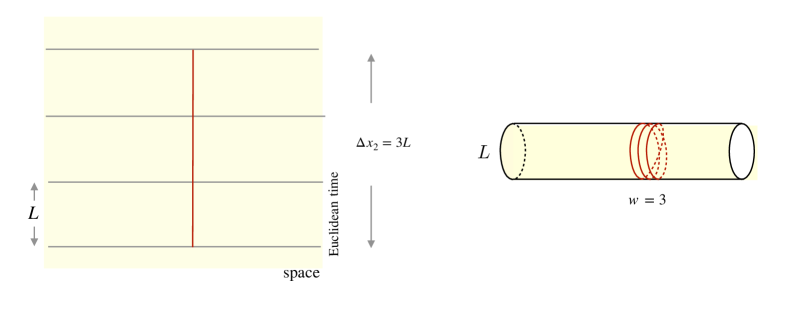
Figure 1: A loop with winding number $w$ as a path integral with a discontinuity $\delta x=\{0,wL\}$ for $w=3$

As for the path integral $[\mathcal{F}^{(L)}]_{0}$ for a contractible loop ($w=0$), it is of the form

$$[\mathcal{F}^{(L)}]_{0}=-RL\epsilon_{0},$$ (2.10)

where $\epsilon_{0}$ is the infinite-volume energy density of the vacuum. The computation of this quantity requires an UV cutoff because the path integral is dominated by small loops. Since the focus here is on the finite-volume effects, a normalisation $\epsilon_{0}=0$ will be assumed for the moment.

2.2 Free massive boson

The free massive boson is defined by the Euclidean path integral

$$\begin{aligned} \mathcal{Z}_{\mathrm{FB}}^{(L)}=\int{\cal D}\varphi\ \exp\left[\int d^{2}x\ \varphi(\nabla^{2}-m^{2})\varphi\right]\end{aligned}$$ (2.11)

with periodic boundary condition $\varphi(x_{1},x_{2}+L)=\varphi(x_{1},x_{2})$. The free energy $\mathcal{F}_{\mathrm{FB}}^{(L)}\equiv\log\mathcal{Z}_{\mathrm{FB}}^{(L)}$ is that of a gas of free oscillators at temperature $1/L$. With the normalisation $\epsilon_{0}=0$,

$$\begin{aligned} \mathcal{F}_{\mathrm{FB}}^{(L)}&=-R\int_{\mathbb{R}}{dp\over 2\pi}\ \log\left(1-e^{-LE_{p}}\right),\qquad E_{p}\equiv\sqrt{p^{2}+m^{2}}\\ &=R\ {\pi\over 6L}\ c_{0}(mL).\end{aligned}$$ (2.12)

The scaling function $c_{0}(mL)$, known as effective central charge, tends in the limit $Lm\to 0$ to the central charge of the Virasoro algebra for a free neutral massless boson,

$$c_{0}(mL)\underset{{m=0}}{\to}-{6L\over\pi}\int_{\mathbb{R}}{dp\over 2\pi}\log(1-e^{-L|p|})=1\,.$$ (2.13)

In the opposite limit, $mL\to\infty$, the effective central charge vanishes.

Now let us obtain the rhs of (2.12) by evaluating the free energy of the grand canonical ensemble of loops embedded in the cylinder. Since the loops do not interact, the free energy is equal to the path integral for a single loop. The path integral contains a sum over all winding numbers

$$\begin{aligned} \mathcal{F}^{(L)}&=\sum_{w\in\mathbb{Z}}\mathcal{F}_{w}^{(L)}\,=2\sum_{w=1}^{\infty}\mathcal{F}_{w}^{(L)}.\end{aligned}$$ (2.14)

After inserting the representation (2.9), the sum over the winding numbers can be done explicitly, with the result

$$\begin{aligned} \mathcal{F}_{\mathrm{FB}}^{(L)}&=-\int_{\mathbb{R}}{Rdp(\theta)\over 2\pi}\ \log\left(1-e^{-LE(\theta)}\right).\end{aligned}$$ (2.15)

This is exactly the free energy of the free massive boson, eq. (2.12).

2.3 Free massive Majorana fermion

In the case of a free massive Majorana fermion, the only new element is the sign factor associated with the intersections of loops. Since any two loops winding around the cylinder intersect each other an even number of times, their intersections do not produce signs. However a loop with winding number $w$ intersects itself $w-1$ times, as illustrated for $w=3$ by fig. 1, hence an extra factor $(-1)^{w-1}$. Taking the signs into account, sum over the winding numbers gives

$$\begin{aligned} \mathcal{F}_{\mathrm{FF}}^{(L)}&=2\sum_{w=1}^{\infty}(-1)^{w-1}\mathcal{F}_{w}\\ &=R\int_{\mathbb{R}}{dp(\theta)\over 2\pi}\ \log\left(1+e^{-LE(\theta)}\right)\equiv{\pi\over 6}{R\over L}\ c_{1/2}(mL).\end{aligned}$$ (2.16)

The effective central charge $c_{1/2}(mL)$ interpolates between $1/2$ in the UV limit and $0$ in the deep IR limit.

The free boson and fermion can be considered as scattering theories with constant scattering factor $\sigma=1$ for the boson and $\sigma=-1$ for the fermion. The expression for the free energy for such a ‘generalised free theory’ is

$$\begin{aligned} \mathcal{F}^{(L)}_{\mathrm{FB,FF}}&=2\sum_{w=1}^{\infty}\sigma^{w-1}\mathcal{F}_{w}^{(L)}\\ &=-\sigma\ \int_{\mathbb{R}}{d\phi(\theta)\over 2\pi}\ \log\left(1-\sigma\,e^{-LE(\theta)}\right),\qquad\phi(\theta)\equiv R\,p(\theta).\end{aligned}$$ (2.17)

The integration measure turns out to be the flat measure for the phase $\phi$ acquired by the one-particle wave function after a tour around the space circle.

2.4 Interacting massive integrable QFT

Now we are prepared to formulate the loop gas for an interacting integrable QFT. In a relativistic integrable QFT with one particle species and no bound states, the scattering matrix $S(p_{1},p_{2})=S(\theta_{1}-\theta_{2})$ is a phase factor satisfying the requirements of real analyticity, unitarity and crossing [1],

$$\begin{aligned} &S(\theta)^{*}=S(-\theta^{*})\qquad\qquad\qquad\text{(real analyticity)}\\ &S(\theta)S(-\theta)=1\qquad\qquad\qquad\qquad\text{(unitarity)}\\ &S(\theta)=S(i\pi-\theta)\qquad\qquad\quad\text{(crossing symmetry)}.\end{aligned}$$ (2.18)

The TBA statistics, bosonic or fermionic, of the particles with the same momenta is determined by the sign of the scattering factor at $\theta=0$,

$$\begin{aligned} \sigma\equiv S(0)=\pm 1.\end{aligned}$$ (2.19)

In the original Yang-Yang paper [4] it is assumed that $\sigma=-1$, but in theories with one space dimension the statistics of identical particles is physically irrelevant because it mixes up with the interaction. It was shown by Wadati [22] that changing both the statistics and the interaction, one can obtain a different description of the same integrable model. Since bosonic S-matrices are known to describe interesting physical phenomena [23, 24], both TBA statistics will be discussed here.

Once the path integral over loops is expressed in terms of on-shell wave functions, eq. (2.7), the loop gas description developed in the previous subsections can be extended to a theory with nontrivial scattering by the following recipe: Intersections of tho segments of loops with rapidities $\theta_{1}$ and $\theta_{2}$ is counted with a factor $S(\theta_{1}-\theta_{2})$.

Scattering factors are associated as well with the self-intersections of a loop. In this case the two segments have coinciding rapidities and the extra factor for a self-intersection is $\sigma=S(0)$.

As any two loops winding around the cylinder intersect an even number of times, the scattering factors compensate thanks to the unitarity property (LABEL:proprsS) of the S-matrix. Therefore the Boltzmann weight for a configuration of $N$ loops with rapidities $\theta_{1},...,\theta_{N}$ factorises into a product of $N$ one-loop Boltzmann weights given by the integrand in (2.9). However the partition function does not exponentiate trivially as in the (generalised) free theory, eq. (2.17), because the rapidities get entangled through the integration measure.

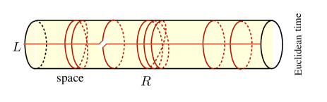
Figure 2: A winding particle touring around the world.

As already mentioned, the measure in the integral over the rapidity is the flat measure for the phase shift $\phi=Rdp(\theta)$ of the semiclassical wave function for distance $R$. The derivative of the phase is proportional to the density of the states in the Hamiltonian description. In an interacting theory, the periodicity condition in $R$ becomes more complicated since the phase shift of the wave function of a particle takes contributions from the scattering with all other particles in the ensemble. One can associate this phase shift with a loop making an extra ‘tour around the world’, as shown in fig 2. The phase acquired after such a trip gets dressed by the scattering factors from crossing the other loops,

$$\phi(\theta|\theta_{1},...,\theta_{N})=Rp(\theta)+i\sum_{k=1}^{N}|w_{k}|\log S(\theta_{k}-\theta).$$ (2.20)

Because of the dressing, the integration measure for $N$ loops does not factorise. The flat measure with respect to the phases $\phi_{1},...,\phi_{N}$ of the $N$ loops,

$$\begin{aligned} \phi_{j}&=Rp(\theta_{j})+i\sum_{k=1}^{N}|w_{k}|\log S(\theta_{k}-\theta_{j}),\ \ \ j=1,...,N,\end{aligned}$$ (2.21)

contains the Jacobian (known as Gaudin determinant [25]) for the change of variables from phases to rapidities,

$$\begin{aligned} \prod_{j=1}^{N}{d\phi_{j}\over 2\pi}=\prod_{j=1}^{N}{d\theta_{j}\over 2\pi}\ \det\left({\partial\phi_{j}\over\partial\theta_{k}}\right).\end{aligned}$$ (2.22)

2.5 Hubbard-Stratonovich fields

The presence of a Jacobian in the integration measure (2.22) has the effect that the free energy becomes a sum of clusters of loops with the structure of branched trees [26, 27]. The generating function for the sum over trees solves the TBA equation. A field-theoretical derivation of the exact cluster expansion was given in [20].

In the context of the loop gas on a cylinder, the effective field theory of [20] arises after a HS type transformation [28, 29] which decouples the two-body interaction of loops. As a result, the ensemble of interacting loops is reformulated as an ensemble of independent loops interacting with a pair of auxiliary fluctuating fields. In order to decouple the interactions, replace in the loop amplitudes

$$\phi(\theta)\equiv Rp(\theta)\ \to\ {{\bm{\phi}}}(\theta),\qquad LE(\theta)\ \to\ \bm{\epsilon}(\theta),$$ (2.23)

where $\bm{\epsilon}(\theta)$ and ${{\bm{\phi}}}(\theta)$ are gaussian holomorphic fields with connected correlation function

$$\begin{aligned} \langle{{\bm{\phi}}}(\theta)\bm{\epsilon}(\theta^{\prime})\rangle_{c}=i\log S(\theta-\theta^{\prime}),\quad\langle\bm{\epsilon}(\theta)\bm{\epsilon}(\theta^{\prime})\rangle_{c}=\langle{{\bm{\phi}}}(\theta){{\bm{\phi}}}(\theta^{\prime})\rangle_{c}=0,\end{aligned}$$ (2.24)

designed to generate the dressing of the phase in (2.20). According to (2.23), the two gaussian fields should be given classical values

$$\begin{aligned} \langle\bm{\epsilon}(\theta)\rangle=LE(\theta),\ \ \ \langle{{\bm{\phi}}}(\theta)\rangle=Rp(\theta).\end{aligned}$$ (2.25)

The path integral over the loops with winding number $w$, eq. (2.9), is now replaced by an operator,

$$\begin{aligned} \mathcal{F}_{w}^{(L)}&={1\over 2}\,\int_{\mathbb{R}}{Rdp(\theta)\over 2\pi}\ {e^{-|w|LE(\theta)}\over|w|}\ \ \to\ \ {\mathbf{F}}_{w}={1\over 2}\,\int_{\mathbb{R}}{d{{\bm{\phi}}}(\theta)\over 2\pi}\ {e^{-|w|\bm{\epsilon}(\theta)}\over|w|}\qquad(w\neq 0).\end{aligned}$$ (2.26)

The ‘operator differential’ $d{{\bm{\phi}}}(\theta)$ has no precise mathematical meaning, but can be given an operational definition as the operator whose expectation value is the differential of the expectation value of the operator ${{\bm{\phi}}}(\theta)$. With this definition, the expectation value

$$\begin{aligned} \left\langle\prod_{j=1}^{N}e^{-|w_{j}|\bm{\epsilon}(\theta_{j})}d{{\bm{\phi}}}(\theta_{j})\right\rangle=\prod_{j=1}^{N}e^{-|w_{j}|LE(\theta_{j})}\prod_{j=1}^{N}{d\phi_{j}\over 2\pi}\end{aligned}$$ (2.27)

generates the Gaudin measure given by the product of the differentials on the lhs of eq. (2.22).

Now the sum over the winding numbers can be performed explicitly, resulting in a remarkably simple operator representation for the partition function,

$$\begin{aligned} {\mathcal{Z}}_{\text{cyl}}^{(L)}=\langle e^{{\mathbf{F}}_{\text{cyl}}}\rangle,\qquad\mathbf{F_{\text{cyl}}}=-\sigma\int_{\mathbb{R}}{d{{\bm{\phi}}}(\theta)\over 2\pi}\ \log\left(1-\sigma e^{-\bm{\epsilon}(\theta)}\right),\end{aligned}$$ (2.28)

with the dependence on $L$ coming from the bare expectation value of $\bm{\epsilon}(\theta)$, eq. (2.25).

However, the simplicity of this expression is deceiving because of the operator differential $d{{\bm{\phi}}}(\theta)$ which requires a precise prescription for calculating the expectation value. Namely, to evaluate the partition function one should first expand the exponential of the free energy operator ${\mathbf{F}}$, and then apply (2.27) term by term. In other words, the evaluation of the partition function (2.28) brings us back to the original sum over interacting loops.

A more manuable operator representation can be constructed by bringing into the game an extra pair of fermionic fields $\bm{\psi}(\theta)$ and $\bm{\eta}(\theta)$ with the same correlation as the bosonic pair,

$$\langle\bm{\xi}(\theta)\bm{\eta}(\theta^{\prime})\rangle=i\log S(\theta-\theta^{\prime}),\qquad\langle\bm{\eta}(\theta)\bm{\eta}(\theta^{\prime})\rangle=\langle\bm{\xi}(\theta)\bm{\xi}(\theta^{\prime})\rangle=0.$$ (2.29)

With the help of the fermionic fields one can amend the operator representation (2.27) so that on the rhs the Gaudin determinant is generated automatically, namely

$$\begin{aligned} \left\langle\prod_{j}e^{-|w_{j}|\bm{\epsilon}(\theta_{j})}\left[\partial{{\bm{\phi}}}(\theta_{j})-|w_{j}|\,{\bm{\eta}}(\theta_{j})\partial{\bm{\xi}}(\theta_{j})\right]\right\rangle&=\prod_{j=1}^{N}e^{-|w_{j}|LE(\theta_{j})}\ \det\left({\partial\phi_{j}\over\partial\theta_{k}}\right).\end{aligned}$$ (2.30)

The proof of this remarkable identity is given in appendix B of [27]. Again, the sum over the winding numbers can be performed explicitly, resulting, together with (2.24) and (2.25), in the operator representation proposed in [20],

$$\begin{aligned} {\mathcal{Z}}_{\text{cyl}}^{(L)}&=\langle e^{{\mathbf{F}}_{\text{cyl}}}\rangle,\qquad\mathbf{F}_{\text{cyl}}=-\sigma\int_{\mathbb{R}}{d\theta\over 2\pi}\ \left[\log\left(1-\sigma e^{-\bm{\epsilon}}\right)\partial_{\theta}{{\bm{\phi}}}+{\bm{\eta}\partial_{\theta}\bm{\xi}\over 1-\sigma\,e^{{\bm{\epsilon}}}}\right].\end{aligned}$$ (2.31)

By obvious reasons, I will refer to ${\mathbf{F}}_{\text{cyl}}$ as the operator of the free energy. The expectation value (2.31) generates, as shown in ref. [20], the exact cluster expansion obtained in [26, 27].

2.6 Ward identities

Let us see how the TBA equation appears. First notice that, since the interaction potential $\mathbf{F}_{\text{cyl}}$ is linear in the field ${{\bm{\phi}}}$, the field $\bm{\epsilon}$ has no dispersion. With the dressed expectation value defined as

$$\langle{\mathcal{O}}\rangle_{\text{cyl}}\equiv{\left\langle{\mathcal{O}}\ e^{{\mathbf{F}}_{\text{cyl}}}\right>\over\left\langle e^{{\mathbf{F}}_{\text{cyl}}}\right>},$$ (2.32)

this means that

$$\left\langle\bm{\epsilon}(\theta)\bm{\epsilon}(\theta^{\prime})\right>_{\text{cyl}}=\left\langle\bm{\epsilon}(\theta)\right>_{\text{cyl}}\left\langle\bm{\epsilon}(\theta^{\prime})\right>_{\text{cyl}}.$$ (2.33)

Furthermore, the fields $\bm{\epsilon}$ and ${{\bm{\phi}}}$ satisfy the obvious Ward identities

$$\left\langle\bm{\epsilon}(\theta)\right>_{{}_{\text{cyl}}} =LE(\theta)+\sigma\,\int_{-\infty}^{\infty}{d\theta^{\prime}\over 2\pi}K(\theta-\theta^{\prime})\left\langle\log\left(1-\sigma\,e^{-\bm{\epsilon}(\theta^{\prime})}\right)\right>_{{\text{cyl}}}\,,$$ (2.34)

$$\left\langle\partial{{\bm{\phi}}}(\theta)\right>_{{\text{cyl}}} =R\partial p(\theta)+\int_{-\infty}^{\infty}{d\theta^{\prime}\over 2\pi}K(\theta-\theta^{\prime})\left\langle{\partial{{\bm{\phi}}}(\theta^{\prime})\over e^{\bm{\epsilon}(\theta^{\prime})}-\sigma}+e^{\epsilon(\theta^{\prime})}{\bm{\eta}(\theta)\partial\bm{\xi}(\theta)\over(e^{\bm{\epsilon}(\theta^{\prime})}-\sigma)^{2}}\right>_{\text{cyl}}\,,$$ (2.35)

where

$$\begin{aligned} K(\theta-\theta^{\prime})&=-\left\langle\partial{{\bm{\phi}}}(\theta)\bm{\epsilon}(\theta^{\prime})\right\rangle_{c}=-i\partial_{\theta}\log S(\theta-\theta^{\prime})\end{aligned}$$ (2.36)

is the scattering kernel.

The Ward identity (2.34), together with the factorisation (2.33), imply a non-linear integral equation for the dressed expectation values $\epsilon(\theta)\equiv\langle\bm{\epsilon}(\theta)\rangle_{{}_{\text{cyl}}}$,

$$\begin{aligned} \epsilon(\theta)&=LE(\theta)+\sigma\,\int_{-\infty}^{\infty}{d\theta^{\prime}\over 2\pi}K(\theta-\theta^{\prime})\log(1-\sigma\,e^{-\epsilon(\theta^{\prime})})\,,\end{aligned}$$ (2.37)

which is identical with the TBA equation for the pseudoenergy.

In the second Ward identity, eq. (2.35), the expectation value contains tree Feynman graphs as well as Feynman graphs with one cycle. The graphs with one cycle produced by the first and by the second term cancel and the Ward identity boils down to a linear integral equation for the dressed scattering phase $\phi(t)\equiv\langle{{\bm{\phi}}}(t)\rangle_{\text{cyl}}$,

$$\begin{aligned} \partial\phi(\theta)&=R\partial p(\theta)+\int_{-\infty}^{\infty}{d\theta^{\prime}\over 2\pi}K(\theta-\theta^{\prime}){\partial\phi(\theta^{\prime})\over e^{\epsilon(\theta^{\prime})}-\sigma}\,,\end{aligned}$$ (2.38)

the meaning of which within the TBA approach will be clarified at the end of this subsection.

From the point of view of Feynman graph expansion of the effective field theory, summarised in appendix A, the non-linear equation for the pseudoenergy sums up the tree Feynman graphs studied in [26, 27]. In this respect the effective field theory is of mean-field type. Indeed, since the interaction potential in eq. (2.31) is linear in ${{\bm{\phi}}}$, the Feynman graph expansion for the free energy stops at one loop. Since the quadratic forms for the gaussian fluctuations of bosons and fermions are the same, the total one-loop contribution vanishes and only tree Feynman graphs survive.

As a consequence, the operator ${\mathbf{F}}_{\text{cyl}}$ is a dispersionless field as well, $\langle\exp{\mathbf{F}}_{\text{cyl}}\rangle=\exp\langle{\mathbf{F}}_{\text{cyl}}\rangle$. This property implies that the partition function is the exponential of the expectation value of the free energy operator ${\mathbf{F}}_{\text{cyl}}$. The computation of the latter is easy,

$$\mathcal{F}_{\text{cyl}}=\langle{\mathbf{F}}_{\text{cyl}}\rangle=-\sigma R\int{d\theta\over 2\pi}\log\left(1-\sigma e^{-\epsilon(\theta)}\right)\partial p(\theta).$$ (2.39)

The rhs is identical to the expression for the free energy obtained in the TBA approach.

To complete the correspondence between the effective field theory and the TBA, let us express, assuming fermionic TBA statistics, $\sigma=-1$, the dressed expectation values $\phi$ and $\epsilon$ in terms of the particle and hole densities $\rho_{p}$ and $\rho_{h}$ as defined in the original paper by Yang and Yang [4]. Obviously expectation value $\epsilon$ corresponds to the pseudoenergy, while the derivative of the phase $\phi$ gives the density of the available states,

$$\begin{aligned} \epsilon&=\log{\rho_{h}\over\rho_{p}},\quad\partial_{\theta}\phi=R(\rho_{p}+\rho_{h}).\end{aligned}$$ (2.40)

Upon this ifentification, the Ward identity for $\epsilon$, eq. (2.37), becomes the TBA equation, as mentioned above, while the Ward identity for ${{\bm{\phi}}}$, eq. (2.38), is equivalent to the linear constraint satisfied by the particle and hole densities (the Bethe equation in terms of densities)

$$\begin{split}\rho_{p}(\theta)+\rho_{h}(\theta)&=\partial\tilde{p}(\theta)+\int_{\mathbb{R}}{d\theta^{\prime}\over 2\pi}K(\theta,\theta^{\prime})\rho_{p}(\theta).\end{split}$$ (2.41)

2.7 One-point function in terms of HS fields

In infinite volume, all matrix elements of a local operator O can be expressed, with the help of the crossing formula, in terms of the infinite-volume elementary form factors

$$F_{n}^{\mathcal{O}}(\theta_{1},...,\theta_{n})=\langle\emptyset|\mathcal{O}|\theta_{1},...,\theta_{n}\rangle.$$ (2.42)

The elementary form factors for local operators satisfy the Watson equations

$$F_{n}(\theta_{1},\dots,\theta_{j},\theta_{j+1},\dots,\theta_{n})=S(\theta_{j},\theta_{j+1})F_{n}(\theta_{1},\dots,\theta_{j+1},\theta_{j},\dots,\theta_{n})$$ (2.43)

and have kinematical singularities

$$F(\theta^{\prime},\theta,\theta_{1},\dots,\theta_{n})={i\over i\pi+\theta^{\prime}-\theta}\left(1-\prod_{j=1}^{n}S(\theta,\theta_{j})\right)F_{n}(\theta_{1},\dots,\theta_{n})+\text{regular}.$$ (2.44)

where it is assumed that the infinite volume states are normalised as $\langle\theta|\theta^{\prime}\rangle=2\pi\delta(\theta-\theta^{\prime})$.

The diagonal limit of the form factors for local operators is not uniform and depend on the prescription. The diagonal matrix elements are given by the connected form factors $F_{2n}^{c}(\theta_{1},\dots,\theta_{n})$ obtained by performing the simultaneous limit $\delta_{1},\dots,\delta_{n}\to 0$. The connected diagonal form factor is obtained by retaining the $\delta$-independent part [8],

$$F_{2n}(i\pi+\theta_{n}+i\delta_{n},\dots,i\pi+\theta_{1}+i\delta_{1},\theta_{1},\dots,\theta_{n})=F_{2n}^{c}(\theta_{1},\dots,\theta_{n})+\ \delta\text{-dependent terms}.\ \ \$$ (2.45)

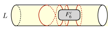
Figure 3: Three loops with winding numbers $w_{1}=2$ and $w_{2}=w_{3}=1$, attached to a connected form factor $F_{6}(\theta_{1},\theta_{2},\theta_{3})$.

Here I will give the field-theoretical equivalent of the derivation presented in [26]. In the loop gas representation, each outgoing particle is identified, after wrapping the cylinder at least once, with the incoming particle with the same rapidity, as shown in fig. 3. The Boltzmann weight of the loops with winding number $w_{1},...,w_{n}$ is given by the expectation value (2.30). The sum over the winding numbers is performed without the symmetry factor $1/|w|$ because there is no more cyclic symmetry. For the fermionic choice $\sigma=-1$, one obtains after summing over the number of particle pairs, the Leclair and Mussardo series [30] for the one-point function of any local operator,

$$\begin{aligned} \langle{\mathcal{O}}\rangle_{\text{cyl}}&=\left\langle\sum_{n=1}^{\infty}{1\over n!}\int\prod_{j=1}^{n}{d\theta_{j}\over 2\pi}\left({1\over e^{\bm{\epsilon}(\theta_{j})}+1}+{e^{\bm{\epsilon}(\theta_{j})}\bm{\eta}(\theta_{j})\partial\bm{\xi}(\theta_{j})\over(e^{\bm{\epsilon}(\theta_{j})}+1)^{2}}\right)F^{c}_{2n}(\theta_{1},\dots,\theta_{n})\right\rangle_{\text{cyl}}\\ &=\sum_{n=1}^{\infty}{1\over n!}\int\prod_{j=1}^{n}{d\theta_{j}\over 2\pi}{1\over e^{\epsilon(\theta_{j})}+1}\ F^{c}_{2n}(\theta_{1},\dots,\theta_{n}),\end{aligned}$$ (2.46)

where the cancellation of the bosonic and the fermionic loops is taken into account. This derivation is of course equivalent to the one by the tree expansion method given in [26]. As for the higher correlation functions, they can be in principle expressed in loop-gas terms, but the interactions of the loops will be more complicated and it is not clear if and how the formalism developed here can be generalised.

3 Generalised free theories on a torus

Before addressing interacting theories, it makes sense to work out the counting and the statistics of the non-interacting loops on the torus. In this section, the partition functions of the generalised free theories, the free neutral massive boson (FB) and the Ising field theory (IFT), will be derived using the loop-gas formulation of these theories. For the FB it is sufficient to compute the path integral of a loop, while the IFT requires some additional combinatorics.

3.1 Path integral for a loop embedded in the torus

Assume that the torus has perpendicular cycles of lengths $L$ and $R$. The generalisation to the case of a tilted torus is mechanical. Let us denote by $[\mathcal{F}^{(L,R)}]_{w,w^{\prime}}$ the path integral for a loop in the topological sector characterised by winding numbers $\{w,w^{\prime}\}$. The explicit expression for this path integral is given by the integral (2.6) over the constant mode of the 2-momentum, with discontinuities $\Delta x_{1}=w^{\prime}R$ and $\Delta x_{2}=wL$, as illustrated in fig. 4,

$$[\mathcal{F}^{(L,R)}]_{w,w^{\prime}}=RL\,\mathcal{F}(\delta\vec{x})\Big{|}_{\delta x_{1}=w^{\prime}R,\delta x_{2}=wL}.$$ (3.1)

Let me remind that the integral (2.6) is obtained from the path integral for loops in infinite volume. If at least one of the winding numbers is non-zero, in the rhs of (3.1) given by the double integral (2.6), one of the integrations can be performed by residues, thus bringing the remaining integral on the mass shell.

$\bullet$ If $\delta x_{2}\neq 0$, the integral with respect to $k_{2}$ can be taken by residues and the integrand takes the form of the wave function of a on-mass-shell particle with momentum $k_{1}$, propagating in the direct channel, analytically continued to imaginary time $t=-i\delta x_{2}$,

$$\begin{aligned} \mathcal{F}(\delta\vec{x})&={\textstyle{1\over 2}}\,{1\over|\delta x_{2}|}\ \int_{\mathbb{R}}{dp(\theta)\over 2\pi}\ e^{-E(\theta)|\delta x_{2}|+ip(\theta)\delta x_{1}}\qquad(\delta x_{2}\neq 0).\end{aligned}$$ (3.2)

$\bullet$ If $\delta x_{1}\neq 0$, one can integrate with respect to $k_{1}$ by residues, with the result that the integrand takes the form of the wave function of on-mass-shell particle propagating in the cross channel, analytically continued to imaginary time $t=-i\delta x_{1}$,

$$\begin{aligned} \mathcal{F}(\delta\vec{x})&={\textstyle{1\over 2}}\,{1\over|\delta x_{1}|}\int_{\mathbb{R}}{dp(\theta)\over 2\pi}\ e^{-E(\theta)|\delta x_{1}|+ip(\theta)\ \delta x_{2}}\qquad(\delta x_{1}\neq 0).\end{aligned}$$ (3.3)

The two wave functions are related by a double Wick rotation exchanging the energy and the momentum, known as mirror transformation,

$$E\to-ip,\ p\to iE$$ (3.4)

or in terms of the rapidity defined in (2.8),

$$\theta\ \to\ \ i\pi/2-\theta.$$ (3.5)

The particles propagating in the direct and in the mirror channels are sometimes referred to a ‘physical’ and ‘mirror’ particles respectively. The mirror transformation (3.5) relates a physical particle with winding numbers $w$ and $w^{\prime}$ and a mirror particle with winding numbers $w^{\prime}$ and $w$.

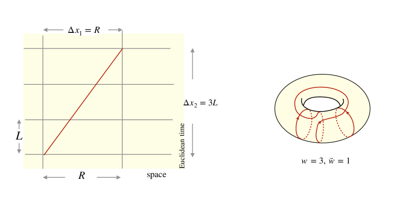
Figure 4: A loop with winding numbers $w,w^{\prime}$ as a path integral with a discontinuity $\delta x=\{w^{\prime}R,wL\}$ for $w=3,w^{\prime}=1$

Thus the path integral $[\mathcal{F}^{(L,R)}]_{w,w^{\prime}}$ admits the following two integral representations,

$$\mathcal{F}_{w,w^{\prime}} \stackrel{{\scriptstyle\text{def}}}{{=}}{{\textstyle{1\over 2}}}R\int_{\mathbb{R}}{dp(\theta)\over 2\pi}{1\over|w|}\ e^{-|w|LE(\theta)+iw^{\prime}Rp(\theta)}\qquad(w\neq 0),$$ (3.6)

$$\tilde{\mathcal{F}}_{w^{\prime},w} \stackrel{{\scriptstyle\text{def}}}{{=}}{{\textstyle{1\over 2}}}L\int_{\mathbb{R}}{dp(\theta)\over 2\pi}{1\over|w^{\prime}|}\ e^{-|w^{\prime}|RE(\theta)+iwLp(\theta)}\qquad(w^{\prime}\neq 0).$$ (3.7)

If $w^{\prime}=0$ or $w=0$, only one of the two representations makes sense. When both winding numbers are non-zero, there is a choice between (3.6) and (3.7). By construction,

$$\mathcal{F}_{w,w^{\prime}}=\tilde{\mathcal{F}}_{w^{\prime},w}\qquad(w,w^{\prime}\neq 0).$$ (3.8)

This identity can be also proved directly by shifting the contour of integration for $\mathcal{F}_{w,w^{\prime}}$ by $i\pi/2$ and integrating by parts. Using the freedom of choice between $\mathcal{F}_{w,w^{\prime}}$ and $\tilde{\mathcal{F}}_{w^{\prime},w}$ when bith winding numbers are non-zero, one can write different integral representations for the free energy of the loop gas.

3.2 Free massive boson

The QFT of a massive bosonic field on the $L\times R$ torus is defined by the Euclidean path integral (2.11) with doubly periodic boundary conditions $\varphi(x_{1}+R,x_{2})=\varphi(x_{1},x_{2})$ and $\varphi(x_{1}+L,x_{2})=\varphi(x_{1},x_{2}).$ The loops being non-interacting, the free energy is equal to the path integral for a single loop. The path integral includes a sum over the topological sectors with winding numbers $w$ and $w^{\prime}$,

$$\begin{aligned} \mathcal{F}_{{\text{FB}}}^{(L,R)}&=\sum_{w,w^{\prime}\in\mathbb{Z}}[\mathcal{F}^{(R,L)}]_{w,w^{\prime}}.\end{aligned}$$ (3.9)

The following three choices for the sum in (3.9) lead to three different integral representations of the free energy of the loop gas,

$$\mathcal{F}^{(L,R)}_{{\text{FB}}} =\sum_{w\neq 0}\mathcal{F}_{w,0}+\sum_{w^{\prime}\neq 0}\sum_{w\in\mathbb{Z}}\tilde{\mathcal{F}}_{w^{\prime},w}$$ (3.10)

$$=\sum_{w^{\prime}\neq 0}\tilde{\mathcal{F}}_{w^{\prime},0}+\sum_{w^{\prime}\in\mathbb{Z}}\sum_{w\neq 0}\mathcal{F}_{w,w^{\prime}}$$ (3.11)

$$=\sum_{w^{\prime}\neq 0}\tilde{\mathcal{F}}_{w^{\prime},0}+\sum_{w\neq 0}\mathcal{F}_{w,0}+{\textstyle{1\over 2}}\sum_{w,w^{\prime}\neq 0}\left(\mathcal{F}_{w,w^{\prime}}+\tilde{\mathcal{F}}_{w^{\prime},w}\right).$$ (3.12)

Let us start with the choice (3.10). The first sum has been calculated in the previous section. In the second double sum, the sum over $w^{\prime}$ gives the periodic delta function $\delta^{(2\pi)}\!\left[L\,p(\theta)\right]$. By substituting the holomorphic representation of the delta function, the second piece is written as a contour integral,

$$\begin{aligned} 2\sum_{w^{\prime}=1}^{\infty}\sum_{w\in\mathbb{Z}}\tilde{\mathcal{F}}_{w^{\prime},w}&=-\oint_{\mathcal{C}_{\mathbb{R}}}\log\left(1-e^{-RE(\theta)}\right)\ {d\log\left(1-e^{iLp(\theta)}\right)\over 2\pi i}\,,\end{aligned}$$ (3.13)

where $\mathcal{C}_{\mathbb{R}}$ is a contour enclosing the real axis,

$$\mathcal{C}_{\mathbb{R}}=\{\overset{-\!-\!\rightarrow}{\mathbb{R}-i0}\}\cup\{\overset{\leftarrow\!-\!-}{\mathbb{R}+i0}\}.$$ (3.14)

Combining the two pieces, one finds for the free energy of the loop gas the following integral expression,

$$\begin{aligned} \mathcal{F}^{(L,R)}_{{\text{FB}}}&=-\int_{\mathbb{R}}{Rdp(\theta)\over 2\pi}\ \log\left(1-e^{-LE(\theta)}\right)-\oint_{\mathcal{C}_{\mathbb{R}}}\log\left(1-e^{-RE(\theta)}\right){d\log\left(1-e^{iLp(\theta)}\right)\over 2\pi i}.\end{aligned}$$ (3.15)

As the integrand of the second term in (3.15) falls exponentially at $\theta\to\pm\infty$, the contour integral can be done by residues, and one obtains the partition function of the massive boson in the form given in [16],

$$\mathcal{Z}_{{\text{FB}}}^{(L,R)}={e^{{\pi\over 6}{R\over L}c_{0}(mL)}\over\prod_{n\in\mathbb{Z}}(1-e^{-RE_{n}})},\quad E_{n}=\sqrt{p_{n}^{2}+m^{2}},\quad p_{n}={2\pi n\over L}.$$ (3.16)

Thus the two integrals in (3.15) have quite different meaning. The first one gives the ground state energy in the cross channel, while the second one takes into account all excited states in the direct channel.

Now let us consider the other two choices, starting with (3.11). Proceeding as above, one arrives at the dual integral representation, obtained from (3.15) by exchanging $L$ and $R$,

$$\begin{aligned} \mathcal{F}^{(R,L)}_{{\text{FB}}}&=-\int_{\mathbb{R}}{Ldp(\theta)\over 2\pi}\ \log\left(1-e^{-RE(\theta)}\right)-\oint_{\mathcal{C}_{\mathbb{R}}}\log\left(1-e^{-LE(\theta)}\right){d\log\left(1-e^{iRp(\theta)}\right)\over 2\pi i}.\end{aligned}$$ (3.17)

In the dual representation, the first term is proportional to the ground-state energy in the direct channel while the second term takes into account the contributions of the excited states in the cross channel.

Finally the third choice, eq. (3.12), gives a self-dual integral representation which can be written, using the mirror transformation (3.5), only in terms of the energy,

$$\begin{aligned} \mathcal{F}^{(L,R)}_{{\text{FB}}}&=-\int\limits_{\mathbb{R}-i0}\log\left(1-e^{-LE(\theta)}\right){d\log\left(1-e^{-RE(i\pi/2-\theta)}\right)\over 2\pi i}+\{L\leftrightarrow R\}.\end{aligned}$$ (3.18)

The equivalence of the three integral representations can be also established directly by deforming the integration contours and then integrating by parts. (There are no surface terms because the integrand decays exponentially at infinity.)

3.3 Ising Field Theory

The IFT is a theory of a bosonic particle describing the order variable of the Ising model in the scaling limit. Its infinite-volume thermodynamics is that of a free Majorana fermion, since both theories describe a free fermionic particle from the TBA perspective. On the torus, however, the IFT is not equivalent to the QFT of a Majorana fermion, as pointed out in [16], although a precise map exists.

The IFT partition function was first computed by Ferdinand and Fischer [31] using the lattice formulation. A field-theoretical derivation (both for the IFT and for the FB) was given by Itzykson and Saleur [15], who computed the zeta-function regularised determinant of the Laplace operator on the torus. Afterwards Klassen and Meltzer [16] expressed, using TBA-related arguments, the results of [15] in a compact and elegant form.

It has been known for a long time that the Ising model can be reformulated as an ensemble of loops. Natalya Vdovichenko [32] found out that the sum over the Ising clusters arising in character expansion of the partition function in the disordered phase ($T>T_{c}$) can be represented as a sum over loops on the lattice with minus signs associated with the intersections. The same reformulation can be done in the ordered phase ($T<T_{c}$), where the clusters are composed of domain walls separating domains of up and down Ising spins. The Boltzmann weights of the loops in the ordered and in the disordered phases are related by the Kramers-Wannier duality [33]. Vdovichenko’s method was generalised to the torus in [34], see also [35]. Again, in the Boltzmann weight of a loop configuration each crossing contributes a factor $(-1)$. Symbolically, the loop gas partition function in the two phases reads (only the sign factors are noted)

$$\begin{aligned} {\mathcal{Z}}^{(L,R)}_{\text{IFT}}&=\sum_{\text{ loops}}(-1)^{\#\text{crossings}}\ \quad\ \ \qquad\qquad\qquad\qquad\qquad(T>T_{c})\\ &=\sum_{\text{ loops}}{\textstyle{1+(-1)^{w_{\mathrm{tot}}}\over 2}{1+(-1)^{w_{\mathrm{tot}}^{\prime}}\over 2}}(-1)^{\#\text{crossings}}\ \ \ \qquad\ \ (T<T_{c}).\end{aligned}$$ (3.19)

In the second line, $w_{\mathrm{tot}}$ and $w_{\mathrm{tot}}^{\prime}$ are the total winding numbers for the two periods of the torus. The extra factor in the ordered low-temperature phase projects to the loop configurations with even total winding numbers in both periods, because periodic boundary conditions for the Ising spins are compatible only with even number of domain walls.

$\bullet$ Derivation of the partition function from the loop gas

The derivation here is along the lines of the lattice derivation given in [34, 35], which simplifies considerably in the continuum limit. To begin with, let us notice that for a loop with winding numbers $\{w,w^{\prime}\}$, the number of times it intersects itself is [11]

$$\#\text{crossings}=w\wedge w^{\prime}-1,\qquad w\wedge w^{\prime}=\text{the greatest common divisor of $w$ and $w^{\prime}$}.$$ (3.20)

By definition $w\wedge 0=w$. Since only the parity of the number of intersections is important, it is convenient to use the identity (for a single loop)

$$(-1)^{\#\text{crossings}}=(-1)^{ww^{\prime}-w-w^{\prime}+1}.$$ (3.21)

From here one infers with little effort that for a configuration of $N$ loops with winding numbers $w_{1},..,w_{N}$ around the $L$-cycle and $w^{\prime}_{1},...,w^{\prime}_{N}$ around the $R$-cycle, the sign factor is

$$\begin{aligned} (-1)^{\#\text{crossings}}\ &=(-1)^{{w_{\mathrm{tot}}w^{\prime}_{\mathrm{tot}}}-{w_{\mathrm{tot}}}-{w^{\prime}_{\mathrm{tot}}}+N}\end{aligned}$$ (3.22)

where $w_{\mathrm{tot}}=w_{1}+...+w_{N}$ and $w^{\prime}_{\mathrm{tot}}=w^{\prime}_{1}+...+w^{\prime}_{N}$. With the help of the identity (3.22), the sign factors in the partition sum (3.19) can expressed solely in terms of the total number of loops and the total winding numbers,

$$\begin{aligned} {\mathcal{Z}}^{(L,R)}_{\text{IFT}}&=\sum_{\text{loops}}(-1)^{w_{\mathrm{tot}}+w_{\mathrm{tot}}^{\prime}+w_{\mathrm{tot}}w_{\mathrm{tot}}^{\prime}}\ (-1)^{\#\text{ loops}}\ \ \ \ \ \ \quad\qquad(T>T_{c}),\\ &=\sum_{\text{loops}}{\textstyle{1+(-1)^{w_{\mathrm{tot}}}\over 2}{1+(-1)^{w_{\mathrm{tot}}^{\prime}}\over 2}}(-1)^{\#\text{ loops}}\ \ \ \quad\qquad\quad\ \ (T<T_{c}).\end{aligned}$$ (3.23)

Unlike the loop gas for the free boson, the sum over loops in (3.23) does not exponentiate because the loops interact through the sign factor $(-1)^{w_{\mathrm{tot}}w_{\mathrm{tot}}^{\prime}}$. Instead, the sum over loops splits into four blocks

$$D_{\alpha\beta}=\sum_{\text{ loops}}e^{2\pi i\alpha w_{\mathrm{tot}}+2\pi i\beta w_{\mathrm{tot}}^{\prime}}\ (-1)^{\#\text{ loops}}\qquad(\alpha,\beta=0,{\textstyle{1\over 2}}),$$ (3.24)

with the sign factor being constant in each block. One verifies immediately, comparing the weights in (3.23) and (3.24), that

$$\begin{aligned} {\mathcal{Z}}^{(L,R)}_{\text{IFT}}\ =\ \ \begin{cases}{\textstyle{1\over 2}}\left(D_{{1\over 2}{1\over 2}}+D_{{1\over 2}0}+D_{0{1\over 2}}-D_{00}\right)&\text{if }\ T>T_{c},\\ {\textstyle{1\over 2}}\left(D_{{1\over 2}{1\over 2}}+D_{{1\over 2}0}+D_{0{1\over 2}}+D_{00}\right)&\text{if }\ T<T_{c}.\end{cases}\end{aligned}$$ (3.25)

The expansion (3.25) of the IFT partition function in four blocks is in accord with [15] for the ordered phase and with [16] for the disordered phase. The different signs of the last term in the two phases have simple explanation. The block $D_{00}$ vanishes at the conformal point $T=T_{c}$ and is linear in $T_{c}-T$ in the scaling regime. Since the partition function at finite volume is analytic in $T$, it must have the same analytic form below and above the critical point. Thus the different signs come from the non-analyticity of the mass $m\sim|T-T_{c}|$.

Let us now compute the four blocks from the loop gas. Since the loops in each block do not interact, the free energy is equal to the path integral for a single loop with sign factors depending on the winding numbers,

$$\begin{aligned} \log D_{\alpha\beta}&=-\sum_{w,w^{\prime}\in\mathbb{Z}}e^{2\pi i\alpha w+2\pi i\beta w^{\prime}}\ [\mathcal{F}^{(R,L)}]_{w,w^{\prime}}.\end{aligned}$$ (3.26)

As in the case of the free boson, there are two natural ways to evaluate the sum, resulting in two integral representations of the rhs analogous to (3.15) and (3.17) for the free boson. For example, the first one reads

$$\begin{aligned} \log D_{\alpha\beta}&=R\int_{\mathbb{R}}{dp(\theta)\over 2\pi}\log\left(1-e^{2\pi i\alpha}e^{-LE(\theta)}\right)\\ &+\oint_{\mathcal{C}_{\mathbb{R}}}\log\left(1-e^{2\pi i\beta}e^{-RE(\theta)}\right){d\log\left(1-e^{2\pi i\alpha}e^{iLp(\theta)}\right)\over 2\pi i}.\end{aligned}$$ (3.27)

In [15, 16], the blocks $D_{\\ a\beta}$ were computed as the partition functions of a Majorana fermion with various boundary conditions. The periodic (Ramond) and the anti-periodic (Neveu-Schwarz) boundary conditions corresponds respectively to $\alpha=0$ and $\alpha={\textstyle{1/2}}$. To connect with [15, 16], one should perform the contour integral in the second line of (3.27) by residues, which gives

$$\begin{aligned} D_{\alpha,\beta}&=e^{-{\pi R\over 6L}\ e^{2\pi i\alpha}c_{\alpha}(mL)}\prod_{n\in\mathbb{Z}+\alpha}\left(1-e^{2\pi i\beta}\ e^{-RE_{n}}\right)\qquad(\alpha,\beta=0,{\textstyle{1\over 2}}).\end{aligned}$$ (3.28)

The scaling function

$$\begin{aligned} c_{\alpha}(mL)=-e^{-2\pi i\alpha}\ {6L\over\pi}\int_{\mathbb{R}}{dp(\theta)\over 2\pi}\log\left(1-e^{2\pi i\alpha}e^{-LE(\theta)}\right)\end{aligned}$$ (3.29)

is the effective central charge in the cross channel for boundary condition $\alpha$, and the product in (3.28) takes into account the excited states in the direct channel. In the UV limit $m\to 0$, the effective central charge tends to its ultraviolet value

$$\begin{aligned} c_{\alpha}(mL)&\underset{{m=0}}{\to}\ =1-\alpha\qquad\quad(\alpha=0,\textstyle{1\over 2}).\end{aligned}$$ (3.30)

In the deep IR limit, $m\to\infty$, there are no degrees of freedom left and the effective central charge vanishes exponentially. The partition function (3.25) in this limit counts the number of the ground states, 1 in the disordered phase and 2 in the ordered phase.

4 Integrable QFT on a torus

4.1 Mapping to a loop gas

After getting the counting and the statistics of the loops straight, one can proceed by switching on the dynamics, as it was done for the theory on a cylinder. Let us consider a non-trivial scattering theory compactified on a rectangular $L\times R$ torus. The claim is that the partition function of an interacting QFT of the type considered in section 2.4 can be computed as the grand partition function of a gas of loops immersed in the torus, with two-body interactions associated with the intersections. Each intersection is counted with a scattering factor which depends on the rapidities of the two intersecting segments of loops.

As was emphasised in section 2.1, the path integral of a winding loop can be expressed in terms of the wave functions either of ‘physical’ on-shell particles propagating in the direct channel, eq. (3.6), or in terms of the wave functions of ‘mirror‘ on-shell particles propagating in the cross channel, eq. (3.7). In what follows, the terms ‘physical particle’ and ‘mirror particle’ applied to a loop will signify which of the two choices is taken.

It became clear from the analysis of the generalised free theories that the loop-gas formulation necessarily involves both physical and mirror particles. When two particles with rapidities $\theta_{1}$ and $\theta_{2}$ have the same kinematics (physical-physical or mirror-mirror), their crossings are weighted by scattering matrix $S(\theta_{1}-\theta_{2})$. When the two particles have different kinematics (physical-mirror or mirror-physical), their crossings are weighted by the scattering factor with one of the arguments mirror-transformed by (3.5). Then the weight is a function of the sum of the two rapidities, $W(\theta_{1}+\theta_{2})$, defined as

$$W(\theta)\stackrel{{\scriptstyle\text{def}}}{{=}}S(\theta-i{\textstyle{\pi\over 2}}).$$ (4.1)

The function $W$ is a real analytic function in the whole $\theta$-plane except for a periodic array of poles on the imaginary axis. It has the symmetries

$$W(\theta)=W(-\theta)=W(\theta+i\pi)^{-1}=W(\theta^{*})^{*},$$ (4.2)

which follow from the unitarity, crossing symmetry and the real analyticity of the S-matrix, eq. (LABEL:proprsS).

Let us give a precise formulation of the statistical ensemble of interacting loops. Take the most general configuration with $N$ particles in the direct channel with rapidities $\theta_{j}$ and winding numbers $\{w_{j},w^{\prime}_{j}\}$, and $\tilde{N}$ particles in the cross channel with rapidities $\tilde{\theta}_{k}$ and winding numbers $\{\tilde{w}_{k},\tilde{w}^{\prime}_{k}\}$. The Boltzmann weight of this configuration is, according to (3.6) and (3.7) ,

$$\begin{aligned} {\mathcal{Z}}^{{N,\tilde{N}}}_{[{\{\theta_{j};w_{j},w^{\prime}_{j}\},\{\tilde{\theta}_{k};{\tilde{w}}_{k},{\tilde{w}}^{\prime}_{k}\}}]}&=\prod_{j=1}^{N}{e^{-L|w_{j}|E(\theta_{j})+iRw^{\prime}_{j}p(\theta_{j})}\over 2|w_{j}|}\prod_{k=1}^{\tilde{N}}{e^{-R|{\tilde{w}}_{k}|E(\tilde{\theta}_{k})+iL{\tilde{w}}^{\prime}_{k}p(\tilde{\theta}_{k})}\over 2|{\tilde{w}}_{k}|}\\ &\times\prod_{j=1}^{N}\sigma^{w_{j}+w^{\prime}_{j}+1}\prod_{k=1}^{\tilde{N}}\sigma^{{\tilde{w}}_{k}+{\tilde{w}}^{\prime}_{k}+1}\\ &\times\prod_{i,j=1}^{N}S(\theta_{i}-\tilde{\theta}_{j})^{|w^{\prime}_{i}|\,w_{j}-|w^{\prime}_{j}|\,w_{i}}\prod_{k,l=1}^{\tilde{N}}S(\theta_{k}-\tilde{\theta}_{l})^{|{\tilde{w}}^{\prime}_{k}|\,{\tilde{w}}_{l}-|{\tilde{w}}^{\prime}_{l}|\,{\tilde{w}}_{k}}\\ &\times\prod_{j=1}^{N}\prod_{k=1}^{\tilde{N}}W(\theta_{j}+\tilde{\theta}_{k})^{-|w_{j}||{\tilde{w}}_{k}|+w^{\prime}_{j}{\tilde{w}}^{\prime}_{k}}S(\theta_{j}-\tilde{\theta}_{k})^{w^{\prime}_{j}|{\tilde{w}}_{k}|-|w_{j}|{\tilde{w}}_{k}^{\prime}}.\end{aligned}$$ (4.3)

Without scattering, the integration measure would be a product of the one-particle integration measures,

$$\prod_{j=1}^{N}{Rdp(\theta_{j})\over 2\pi}\prod_{k=1}^{\tilde{N}}{Ldp(\tilde{\theta}_{k})\over 2\pi}=\prod_{j=1}^{N}d\phi_{j}\prod_{k=1}^{\tilde{N}}d\tilde{\phi}_{k}\,,$$ (4.4)

where the rhs is expressed through the phase shifts of the wave functions of the physical and the mirror particles. If both $L$ and $R$ are large, the measure is again the flat measure for the phase shifts which now have contribution from the scattering

$$\begin{aligned} \phi_{j}&=Rp(\theta_{j})-i\sum_{j^{\prime}=1}^{N}|w_{j^{\prime}}|\log S(\theta_{j}-\theta_{j^{\prime}})-i\sum_{k=1}^{\tilde{N}}{\tilde{w}}^{\prime}_{k}\log W(\theta_{j}+\tilde{\theta}_{k}),\quad(j=1,...,N)\\ \tilde{\phi}_{k}&=Lp(\tilde{\theta}_{k})-i\sum_{j=1}^{N}w^{\prime}_{j}\log W(\tilde{\theta}_{k}+\theta_{j})-i\sum_{k^{\prime}=1}^{\tilde{N}}|\tilde{w}_{k^{\prime}}|\log S(\tilde{\theta}_{k}-\tilde{\theta}_{k^{\prime}})\quad(k=1,...,\tilde{N}).\end{aligned}$$ (4.5)

Since all winding effects are already taken into account, it is plausible that the expression (4.4) holds also for finite $R$ and $L$, although I do not know if a rigorous proof can be constructed at all. With no proof available, the expression (4.4) should be considered as a definition of the measure for the loop gas.

With the measure thus defined, the contribution to the partition function of the collection of loops with this particular topology is given by the integral of the $N+\tilde{N}$ rapidities

$$\begin{aligned} {\mathcal{Z}}^{{N,\tilde{N}}}_{[{\{w_{j},w^{\prime}_{j}\},\{{\tilde{w}}_{k},{\tilde{w}}^{\prime}_{k}\}}]}&=\ \int\limits_{\mathbb{R}^{N+\tilde{N}}}{\mathcal{Z}}^{{N,\tilde{N}}}_{[{\{\theta_{j};w_{j},w^{\prime}_{j}\},\{\tilde{\theta}_{k};{\tilde{w}}_{k},{\tilde{w}}^{\prime}_{k}\}}]}\ \prod_{j=1}^{N}{d\phi_{j}\over 2\pi}\prod_{k=1}^{\tilde{N}}{d\tilde{\phi}_{k}\over 2\pi},\end{aligned}$$ (4.6)

with $\phi_{j}$ and $\tilde{\phi}_{k}$ given by (4.5). The integration measure contains a Jacobian for the change of variables from $\{\phi,\tilde{\phi}\}$ to $\{\theta,\tilde{\theta}\}$:

$$\begin{aligned} \prod_{j=1}^{N}{d\phi_{j}}\prod_{k=1}^{\tilde{N}}{d\tilde{\phi}_{k}}=\prod_{j=1}^{N}{d\theta_{j}}\prod_{k=1}^{\tilde{N}}{d\tilde{\theta}_{k}}\ \det\left(\begin{array}[]{cc}{\partial\phi_{j}/\partial\theta_{j^{\prime}}}&{\partial\phi_{j}/\partial\tilde{\theta}_{k}}\\ {\partial\tilde{\phi}_{k}/\partial\theta_{j}}&{\partial\tilde{\phi}_{k}/\partial\tilde{\theta}_{k^{\prime}}}\end{array}\right).\end{aligned}$$ (4.7)

The loop amplitudes of the type (4.3) split into equivalence classes related by mirror transformations with respect to part of the rapidities. The grand canonical partition functions must contain only one representative of each class. A possible choice for the sum, corresponding to the choice (3.10) for the free boson, is

$$\begin{aligned} {\mathcal{Z}}^{(L,R)}_{\text{tor}}&=\sum_{N,\tilde{N}=0}^{\infty}\sum_{\{w_{j}\neq 0\}}\sum_{\{{\tilde{w}}_{k}\neq 0,{\tilde{w}}^{\prime}_{k}\}}\ {{\mathcal{Z}}^{N,\tilde{N}}_{[{\{w_{j},0\},\{{\tilde{w}}_{k},{\tilde{w}}^{\prime}_{k}\}}]}\over N!\ \tilde{N}!}\\ &\underset{S=1}{\to}\exp\left(\sum_{w\neq 0}\mathcal{F}_{w,0}+\sum_{{\tilde{w}}^{\prime}\neq 0}\sum_{{\tilde{w}}\in\mathbb{Z}}\tilde{\mathcal{F}}_{w^{\prime},w}\right).\end{aligned}$$ (4.8)

4.2 The partition function in terms of HS fields

The effective QFT for the torus can be constructed as a generalisation of the operator representation (2.28) for the cylinder. To achieve a symmetric description of the direct and the cross channels, it is convenient to introduce special notations for the mirror images of fields $\bm{\epsilon}$ and ${{\bm{\phi}}}$ defined in section (2.5),

$${{\bm{\tilde{\phi}}}}(\theta)\equiv i\bm{\epsilon}(i\pi/2-\theta),\qquad{\bm{\tilde{\epsilon}}}(\theta)\equiv-i{{\bm{\phi}}}(i\pi/2-\theta).$$ (4.9)

The HS fields are designed to generate the scattering factors in (4.3). For that they should have the following two-point functions,

$$\begin{aligned} &\langle{{\bm{\phi}}}(\theta)\bm{\epsilon}(\theta^{\prime})\rangle_{c}=\langle{{\bm{\tilde{\phi}}}}(\theta){\bm{\tilde{\epsilon}}}(\theta^{\prime})\rangle_{c}=i\log S(\theta-\theta^{\prime})\,,\\ &\langle\bm{\epsilon}(\theta)\tilde{\bm{\epsilon}}(\theta^{\prime})\rangle_{c}=\langle{{\bm{\phi}}}(\theta){{\bm{\tilde{\phi}}}}(\theta^{\prime})\rangle_{c}=-\log W(\theta+\theta^{\prime})\,,\\ &\langle\bm{\epsilon}(\theta)\bm{\epsilon}(\theta^{\prime})\rangle_{c}=\langle{{\bm{\phi}}}(\theta){{\bm{\phi}}}(\theta^{\prime})\rangle_{c}=\langle{\bm{\tilde{\epsilon}}}(\theta){\bm{\tilde{\epsilon}}}(\theta^{\prime})\rangle_{c}=\langle{{\bm{\tilde{\phi}}}}(\theta){{\bm{\tilde{\phi}}}}(\theta^{\prime})\rangle_{c}=\langle\bm{\epsilon}(\theta){{\bm{\tilde{\phi}}}}(\theta^{\prime})\rangle_{c}=\langle{\bm{\tilde{\epsilon}}}(\theta){{\bm{\phi}}}(\theta^{\prime})\rangle_{c}=0.\end{aligned}$$ (4.10)

Of course, the propagators involving $\tilde{\bm{\epsilon}}$ and $\tilde{{\bm{\phi}}}$ follow from the definition (4.9). The asymptotic energies and momenta are introduced as classical values of the HS fields,

$$\langle\bm{\epsilon}(\theta)\rangle=LE(\theta),\ \ \ \langle{{\bm{\phi}}}(\theta)\rangle=Rp(\theta),\quad\langle{\bm{\tilde{\epsilon}}}(\theta)\rangle=RE(\theta),\ \ \ \langle{{\bm{\tilde{\phi}}}}(\theta)\rangle=Lp(\theta)\,.$$ (4.11)

From the properties of the two-point correlators and the classical values it follows that the HS fields are real analytic and anti-periodic with respect to $\theta\to\theta+i\pi$. This will be used later to construct oscillator representation of the HS fields associated with their expansions in the odd powers of $e^{\theta}$.

The path integrals for loops with winding numbers $w,w^{\prime}$, evaluated in physical and in mirror kinematics, eqs. (3.6) and (3.7), are now replaced respectively by the operators

$${\mathbf{F}}_{w,w^{\prime}} ={\textstyle{1\over 2}}\,\sigma^{w+w^{\prime}-1}\int_{\mathbb{R}}{d{{\bm{\phi}}}(\theta)\over 2\pi}{1\over|w|}\ e^{-|w|\bm{\epsilon}(\theta)+iw^{\prime}{{\bm{\phi}}}(\theta)}\qquad(w\neq 0)$$ (4.12)

$$\tilde{\mathbf{F}}_{w^{\prime},w} ={\textstyle{1\over 2}}\,\sigma^{w+w^{\prime}-1}\int_{\mathbb{R}}{d{{\bm{\tilde{\phi}}}}(\theta)\over 2\pi}{1\over|w^{\prime}|}\ e^{-|w^{\prime}|{\bm{\tilde{\epsilon}}}(\theta)+iw{{\bm{\tilde{\phi}}}}(\theta)}\qquad(w^{\prime}\neq 0).$$ (4.13)

The operators ${\mathbf{F}}_{w,w^{\prime}}$ and $\tilde{\mathbf{F}}_{w^{\prime},w}$ satisfy the operator analogue of the duality relation (3.8),

$${\mathbf{F}}_{w,w^{\prime}}=\tilde{\mathbf{F}}_{w^{\prime},w}\qquad(w,w^{\prime}\neq 0),$$ (4.14)

which can be proved as (3.8) by shifting the contour of integration on the lhs by $i\pi/2$ and integrating by parts.

Now the integral (4.6) takes the form of the following expectation value

$$\begin{aligned} {\mathcal{Z}}_{\{w_{j},w^{\prime}_{j}\},\{{\tilde{w}}_{k},{\tilde{w}}^{\prime}_{k}\}}&=\left\langle\prod_{j=1}^{N}{\mathbf{F}}_{w_{j},w^{\prime}_{j}}\prod_{j=1}^{N}\tilde{\mathbf{F}}_{\tilde{w}_{j},\tilde{w}^{\prime}_{j}}\right\rangle.\end{aligned}$$ (4.15)

To express the operator differentials in terms of derivatives, one can proceed as in section 2.5 by introducing Faddeev-Popov ghosts. Now we have two pairs of fermions $\{\bm{\psi},\bm{\eta}\}$ with the same two-point functions as the bosons with correlation functions,

$$\begin{aligned} \langle\bm{\eta}(\theta)\bm{\xi}(\theta^{\prime})\rangle&=\langle{\bm{\tilde{\eta}}}(\theta){\bm{\tilde{\psi}}}(\theta^{\prime})\rangle=i\log S(\theta-\theta^{\prime}),\\ \langle\bm{\eta}(\theta){\bm{\tilde{\psi}}}(\theta^{\prime})\rangle&=\langle{\bm{\tilde{\eta}}}(\theta)\bm{\xi}(\theta^{\prime})\rangle=i\log W(\theta+\theta^{\prime}).\end{aligned}$$ (4.16)

The fermions ${\bm{\tilde{\eta}}}$ and ${\bm{\tilde{\psi}}}$ are mirror images of $\bm{\psi}$ and ${\bm{\tilde{\psi}}}$,

$${\bm{\tilde{\eta}}}(\theta)\equiv\bm{\xi}(i\pi/2-\theta),\qquad{\bm{\tilde{\psi}}}(\theta)\equiv\bm{\eta}(i\pi/2-\theta).$$ (4.17)

The fermionic representation of the Jacobian on the rhs of (4.7) is a straightforward generalisation of eq. (2.30). If the product of differentials in the expectation value in (4.15) is replaced as

$$\begin{aligned} \prod_{j=1}^{N}{d\ {{\bm{\phi}}}_{j}\over 2\pi}\prod_{k=1}^{\tilde{N}}{d\tilde{{\bm{\phi}}}_{k}\over 2\pi}&\to\ \prod_{j=1}^{N}{d\ \theta_{j}\over 2\pi}\prod_{k=1}^{\tilde{N}}{d\tilde{\theta}^{\prime}_{k}\over 2\pi}\\ &\times\prod_{j=1}^{N}{\partial{{\bm{\phi}}}(\theta_{j})-|w_{j}|\,\bm{\eta}(\theta_{j})\partial\bm{\xi}(\theta_{j})\over 2\pi}\ {\partial{{\bm{\tilde{\phi}}}}(\theta^{\prime}_{k})-|w^{\prime}_{k}|\,{\bm{\tilde{\eta}}}(\theta^{\prime}_{k})\partial\bm{\tilde{\xi}}(\theta^{\prime}_{k})\over 2\pi},\end{aligned}$$ (4.18)

then the expectation value of the rhs gives the Jacobian on the rhs of (4.7). The corresponding expressions for the operator loop amplitudes (4.12) and (4.13) are

$$\begin{aligned} {\mathbf{F}}_{w,w^{\prime}}&={\textstyle{1\over 2}}\,\sigma^{w+w^{\prime}-1}\int_{\mathbb{R}}{d\theta\over 2\pi}\ e^{-|w|\bm{\epsilon}+iw^{\prime}{{\bm{\phi}}}}\left({\partial_{\theta}{{\bm{\phi}}}\over|w|}-\bm{\eta}\partial_{\theta}\bm{\xi}\right)\qquad(w\neq 0)\\ \tilde{\mathbf{F}}_{w,w^{\prime}}&={\textstyle{1\over 2}}\,\sigma^{w+w^{\prime}-1}\int_{\mathbb{R}}{d\theta\over 2\pi}\ e^{-|w|{\bm{\tilde{\epsilon}}}+iw^{\prime}{{\bm{\tilde{\phi}}}}}\left({\partial_{\theta}{{\bm{\tilde{\phi}}}}\over|w|}-{\bm{\tilde{\eta}}}\partial_{\theta}\bm{\tilde{\xi}}\right)\qquad(w\neq 0).\end{aligned}$$ (4.19)

The sum over the winding numbers can be performed explicitly as in the case of the free theory. The partition function is equal to the expectation value

$$\mathcal{Z}_{\text{tor}}^{(L,R)}=\langle e^{\mathbf{F}_{\text{tor}}}\rangle,$$ (4.20)

where the operator ${\mathbf{F}}_{\text{tor}}$ can be given different integral representations depending on the choice physical/mirror for the winding loop kinematics. Performing the sum as in (3.10), one obtains

$$\begin{aligned} {\mathbf{F}}_{\text{tor}}=&-\sigma\int_{\mathbb{R}}{d\theta\over 2\pi}\left[\log\left(1-\sigma e^{-\bm{\epsilon}}\right)\partial_{\theta}{{\bm{\phi}}}\,+{\bm{\eta}\partial_{\theta}\bm{\xi}\over 1-\sigma\,e^{{\bm{\epsilon}}}}\right]\\ &-\sigma\oint_{\mathcal{C}_{\mathbb{R}}}{d\theta\over 2\pi}{1\over 1-\sigma e^{-i{{\bm{\tilde{\phi}}}}}}\left[\log\left(1-\sigma\,e^{-{\bm{\tilde{\epsilon}}}}\right){\partial_{\theta}{{\bm{\tilde{\phi}}}}}+{{\bm{\tilde{\eta}}}\partial_{\theta}\bm{\tilde{\xi}}\over 1-\sigma e^{{{\bm{\tilde{\epsilon}}}}}}\right]\,.\end{aligned}$$ (4.21)

The dual representation, which corresponds to the sum as in (3.11) and is mirror image of the first, reads

$$\begin{aligned} \mathbf{F}_{\mathrm{tor}}=&-\sigma\int\limits_{\mathbb{R}}{d\theta\over 2\pi}\left[\log\left(1-\sigma e^{-{\bm{\tilde{\epsilon}}}(\theta)}\right)\partial_{\theta}{{\bm{\tilde{\phi}}}}+{{\bm{\tilde{\eta}}}\partial_{\theta}\bm{\tilde{\xi}}\over 1-\sigma e^{{{\bm{\tilde{\epsilon}}}}}}\right]\\ &-\sigma\oint\limits_{\mathcal{C}_{\mathbb{R}}}{d\theta\over 2\pi}{1\over 1-\sigma e^{-i\varphi}}\left[\log\left(1-\sigma\,e^{-\bm{\epsilon}}\right){\partial_{\theta}\varphi}+{\bm{\eta}\partial_{\theta}\bm{\xi}\over 1-\sigma e^{{\bm{\epsilon}}}}\right].\end{aligned}$$ (4.22)

The operator ${\mathbf{F}}_{\text{tor}}$ can be treated as the interaction potential in a standard quantum field theory. In particular, one can set up a Feynman diagram expansion of the free energy above the mean-field given by the TBA equation. The integral representation (4.21) of the interaction potential is best suited for calculating the exponential corrections to the TBA solution when $L$ is finite and $R$ is large. The exponential corrections in this limit come from the second line in (4.21). In the opposite limit where $L$ is large and $R$ is finite, one can use the dual integral representation (4.22).

Let us describe qualitatively the diagram technique, cf. appendix A. It makes sense to expand around the mean-field solution in order to avoid summing over trees. The mean-field solution which is determined by a pair of non-linear integral equations

$$\begin{aligned} \epsilon(\theta)&=LE(\theta)-\int_{-\infty}^{\infty}{d\theta^{\prime}\over 2\pi}K(\theta-\theta^{\prime})\log\left(1+e^{-\epsilon(\theta^{\prime})}\right)\\ &-\oint\limits_{\mathcal{C}_{\mathbb{R}}}{d\theta^{\prime}\over 2\pi}\log W(\theta+\theta^{\prime}){\partial_{\theta}\tilde{\phi}(\theta^{\prime})\over(1+e^{-i\tilde{\phi}})(1+\,e^{-\tilde{\epsilon}(\theta^{\prime})})}\,\\ {{\bm{\phi}}}(\theta)&=Rp(\theta)+i\int_{-\infty}^{\infty}{d\theta^{\prime}\over 2\pi}\log S(\theta-\theta^{\prime}){\partial\phi(\theta^{\prime})\over 1+e^{\epsilon(\theta^{\prime})}}\,\\ &-\oint\limits_{\mathcal{C}_{\mathbb{R}}}{d\theta^{\prime}\over 2\pi}\log W(\theta+\theta^{\prime}){\partial\tilde{\epsilon}(\theta^{\prime})\over(1+e^{\tilde{\epsilon}(\theta^{\prime})})(1+e^{-i\tilde{\phi}(\theta^{\prime})})},\\ \tilde{\epsilon}(\theta)&=-i\phi(i\pi/2-\theta),\quad\tilde{\phi}(\theta)=i\epsilon(i\pi/2-\theta).\end{aligned}$$ (4.23)

The difference with the (exact) mean-field equations in the TBA limit, (2.37) and (2.38), is in the last terms, which reflect the presence of excited stated in the cross channel. The connected vacuum Feynman graphs have at least one loop. The total contribution of the graphs with only one loop vanishes because of the cancellations between bosons and fermions. More generally, the contribution of a graph containing a bosonic loop which is simply connected to the rest of the graph, is compensated by a similar graph containing a fermionic loop.

4.3 TBA limit and excited states

Let us see how the expectation value (4.20) generates the sum over all excited states in the cross channel. Choose fermionic TBA statistics, $\sigma=-1$. In the limit of $Rm$ large and $Lm$ finite, the operator $e^{{\mathbf{F}}_{\text{tor}}}$ can be expanded in a series in $e^{-{\bm{\tilde{\epsilon}}}}\sim e^{-mR}$ with leading term $e^{{\mathbf{F}}_{\text{cyl}}}$,

$$\begin{aligned} e^{\mathbf{F}_{\text{tor}}}&=e^{\mathbf{F}_{\text{cyl}}}+e^{\mathbf{F}_{\text{cyl}}}\oint\limits_{\mathcal{C}_{\mathbb{R}}}{d\theta\over 2\pi i}\left(e^{-{\bm{\tilde{\epsilon}}}(\theta)}-{1\over 2}e^{-2{\bm{\tilde{\epsilon}}}(\theta)}\right)\partial_{\theta}\log\left(1+e^{i{{\bm{\tilde{\phi}}}}(\theta)}\right)\\ &+{1\over 2!}e^{\mathbf{F}_{\text{cyl}}}\oint\limits_{\mathcal{C}_{\mathbb{R}}\times\mathcal{C}_{\mathbb{R}}}{d\theta\over 2\pi i}{d\theta^{\prime}\over 2\pi i}e^{-{\bm{\tilde{\epsilon}}}(\theta)}\,e^{-{\bm{\tilde{\epsilon}}}(\theta^{\prime})}\partial_{\theta}\log\left(1+e^{i{{\bm{\tilde{\phi}}}}(\theta)}\right)\partial_{\theta^{\prime}}\log\left(1+e^{i{{\bm{\tilde{\phi}}}}(\theta^{\prime})}\right)+....\end{aligned}$$ (4.24)

The integral in the subleading order ($\sim e^{-{\bm{\tilde{\epsilon}}}}$), evaluated by residues, gives the sum of one-particle excited states in the cross channel whose rapidity $\theta$ are determined by the poles of the integrand,

$$\left\langle e^{\mathbf{F}_{\text{cyl}}}\,e^{-{\bm{\tilde{\epsilon}}}(\theta)}\left(1+e^{i{{\bm{\tilde{\phi}}}}(\theta)}\right)\right\rangle=0\quad\Rightarrow\theta.$$ (4.25)

The next order ($\sim e^{-2{\bm{\tilde{\epsilon}}}}$) consists of two terms representing a single and a double integral. The double integral gives a sum over the two-particle excited states characterised by pairs of residues at $\theta_{1}$ and $\theta_{2}$ such that

$$\left\langle e^{\mathbf{F}_{\text{cyl}}}e^{-{\bm{\tilde{\epsilon}}}(\theta_{1})-{\bm{\tilde{\epsilon}}}(\theta_{2})}\left(1+e^{i{{\bm{\tilde{\phi}}}}(\theta_{1})}\right)\right\rangle=\left\langle e^{\mathbf{F}_{\text{cyl}}}e^{-{\bm{\tilde{\epsilon}}}(\theta_{1})-{\bm{\tilde{\epsilon}}}(\theta_{2})}\left(1+e^{i{{\bm{\tilde{\phi}}}}(\theta_{2})}\right)\right\rangle=0.$$ (4.26)

The contribution of the unphysical excited state with $\theta_{1}=\theta_{2}$ is compensated by the single integral.

In the sector with $N$-particle excited states, the spectrum of the rapidities $\theta_{1},...,\theta_{N}$ is determined by the positions of the $N$ poles of the integrand, which are determined by the conditions

$$\begin{aligned} \tilde{\phi}_{j}\equiv{\langle{{\bm{\tilde{\phi}}}}(\theta_{j})\prod_{k=1}^{N}e^{-{\bm{\tilde{\epsilon}}}(\theta_{k})}\ e^{{\mathbf{F}}_{\text{tor}}}\rangle\over\langle\prod_{k=1}^{N}e^{-{\bm{\tilde{\epsilon}}}(\theta_{k})}\ e^{{\mathbf{F}}_{\text{tor}}}\rangle}=2\pi I_{k}+\pi,\quad k=1,...,N.\end{aligned}$$ (4.27)

with $I_{k}$ integer numbers. The explicit expressions for the phases $\tilde{\phi}_{k}$ are

$$\begin{aligned} \tilde{\phi}_{j}=mLp(\theta_{j})-i\sum_{k=1}^{N}\log S(\theta_{j}-\theta_{k})+\int{d\theta\over 2\pi}\log(1+e^{-\epsilon(\theta)})\ \partial_{\theta}\log W(\theta+\theta_{j})\end{aligned}$$ (4.28)

where the pseudoenergy $\epsilon(\theta)$ satisfies the integral equation

$$\begin{aligned} \epsilon(\theta)&={\langle\bm{\epsilon}(\theta)\prod_{k=1}^{N}e^{-{\bm{\tilde{\epsilon}}}(\theta_{k})}\ e^{{\mathbf{F}}_{\text{tor}}}\rangle\over\langle\prod_{k=1}^{N}e^{-{\bm{\tilde{\epsilon}}}(\theta_{k})}\ e^{{\mathbf{F}}_{\text{tor}}}\rangle}\\ &=RE(\theta)+\sum_{k=1}^{N}\log W(\theta+\theta_{k})-\int_{\mathbb{R}}{d\theta^{\prime}\over 2\pi}K(\theta-\theta^{\prime})\log(1+e^{-\epsilon(\theta^{\prime})}).\end{aligned}$$ (4.29)

The partition function in presence of the $N$-particle excited state with quantum numbers $I_{1},...,I_{N}$ is

$$\begin{aligned} {\mathcal{Z}}_{I_{1},...,I_{N}}&=\prod_{j}e^{-RE(\theta_{j})}\ e^{R\int{dp(\theta)\over 2\pi}\log(1+e^{-\epsilon(\theta)})}\qquad(I_{1}\leq...\leq I_{N}).\end{aligned}$$ (4.30)

Although the quantisation numbers can coincide, the rapidities of the multi-particle excited states are all different, $\theta_{1}<...<\theta_{N}$, because of the cancellations discussed above. The quantisation conditions (4.28)-(4.29) were derived for the sinh-Gordon model by analytical continuations of the ground state TBA in [36], and using a lattice realisation of the theory in [37].

4.4 Oscilator representation of the cylinder and torus partition functions

In this section, the HS fields will be given a standard representation in terms of creation and annihilation operators of bose and fermi type acting in a Fock space. The bosonic fields $\{\bm{\epsilon},{{\bm{\phi}}}\}$ and their mirrors $\{{\bm{\tilde{\epsilon}}},{{\bm{\tilde{\phi}}}}\}$ will be expressed in terms of a free complex chiral boson $\{{\bm{\varphi}},{\bm{\bar{\varphi}}}\}$ as

$$\begin{aligned} \bm{\epsilon}(\theta)&={\bm{\varphi}}(\theta),\quad\ \ \ {{\bm{\phi}}}(\theta)=i{\bm{\bar{\varphi}}}(\theta-i\pi/2),\\ {\bm{\tilde{\epsilon}}}(\theta)&={\bm{\bar{\varphi}}}(-\theta),\quad{{\bm{\tilde{\phi}}}}(\theta)=i{\bm{\varphi}}(-\theta+i\pi/2).\end{aligned}$$ (4.31)

The fermionic fields $\{\bm{\eta},\bm{\psi}\}$ and their mirrors $\{{\bm{\tilde{\eta}}},{\bm{\tilde{\psi}}}\}$ will be expressed in terms of a free complex chiral fermion $\{\bm{\psi},\bm{\bar{\psi}}\}$ as

$$\begin{aligned} \bm{\xi}(\theta)&=\bm{\psi}(\theta),\quad\ \ \ \bm{\eta}(\theta)=i\bm{\bar{\psi}}(\theta-i\pi/2),\\ \bm{\tilde{\xi}}(\theta)&=\bm{\bar{\psi}}(-\theta),\quad{\bm{\tilde{\eta}}}(\theta)=i\bm{\psi}(-\theta+i\pi/2).\end{aligned}$$ (4.32)

$\bullet$ Fock space

The bosonic field is defined by the mode expansion at $\theta\to\pm\infty$

$$\begin{aligned} {\bm{\varphi}}(\theta)&=\sum_{n\ \mathrm{odd}}\mathbf{a}_{n}\ {e^{-n\theta}\over n}\,,\quad{\bm{\bar{\varphi}}}(\theta)=\sum_{n\ \mathrm{odd}}\bar{\mathbf{a}}_{n}\,{e^{-n\theta}\over n}\,,\end{aligned}$$ (4.33)

with the operator amplitudes satisfying the commutation relations

$$[\mathbf{a}_{n},\mathbf{\bar{a}}_{m}]=-nW_{n}\delta_{m+n,0}\,,\qquad[\mathbf{a}_{m},\mathbf{a}_{n}]=[\mathbf{\bar{a}}_{m},\mathbf{\bar{a}}_{n}]=0\qquad(n,m=\text{odd})$$ (4.34)

in which the coefficients $W_{n}$ are determined by the expansion of the function $\log W(\theta)$ at $\theta\to\pm\infty$,

$$\begin{aligned} \log W(\theta)&=\sum_{k\geq 1,\text{odd}}^{\infty}{W_{n}\over n}\,e^{-n\theta}\qquad(\Re\theta>0)\\ &=\sum_{k\geq 1,\text{odd}}^{\infty}{W_{n}\over n}\,e^{n\theta}\qquad(\Re\theta<0).\end{aligned}$$ (4.35)

This is the general form of the expansion for a purely elastic scattering matrices [38]. The left and right Fock vacua are defined by

$$\langle 0|0\rangle=1,\quad\langle 0|\mathbf{a}_{-n}=\langle 0|\bar{\mathbf{a}}_{-n}=\mathbf{a}_{n}|0\rangle=\bar{\mathbf{a}}_{n}|0\rangle=0\quad\ \ (n>0).$$ (4.36)

Similarly, the fermionic field is defined by

$$\begin{aligned} \bm{\psi}(\theta)&=\sum_{n\ \mathrm{odd}}\mathbf{b}_{n}\ {e^{-n\theta}\over n}\,,\quad\bm{\bar{\psi}}(\theta)=\sum_{n\ \mathrm{odd}}\mathbf{\bar{b}}_{n}\,{e^{-n\theta}\over n}\,,\end{aligned}$$ (4.37)

$$[\mathbf{b}_{n},\mathbf{\bar{b}}_{m}]_{+}=-nW_{n}\delta_{m+n,0}\,,\qquad[\mathbf{b}_{m},\mathbf{b}_{n}]_{+}=[\mathbf{\bar{b}}_{m},\mathbf{\bar{b}}_{n}]_{+}=0\qquad(n,m=\text{odd})$$ (4.38)

$$\langle 0|0\rangle=1,\quad\langle 0|\mathbf{b}_{-n}=\langle 0|\mathbf{\bar{b}}_{-n}=\mathbf{b}_{n}|0\rangle=\mathbf{\bar{b}}_{n}|0\rangle=0\quad\ \ (n>0).$$ (4.39)

$\bullet$ Two-point functions

The commutation relations (4.34) and (4.38) are designed so that

$$\langle 0|{\bm{\varphi}}(\theta){\bm{\bar{\varphi}}}(\theta^{\prime})|0\rangle=\langle 0|\bm{\psi}(\theta)\bm{\bar{\psi}}(\theta^{\prime})|0\rangle=-\sum_{n\geq 1,\text{odd}}{W_{n}\over n}e^{-n(\theta+\theta^{\prime})}=-\log W(\theta+\theta^{\prime}).$$ (4.40)

The two-point function for the bosons does not depend on the order of the operators,

$$\langle 0|{\bm{\varphi}}(\theta){\bm{\bar{\varphi}}}(\theta^{\prime})|0\rangle=\langle 0|{\bm{\bar{\varphi}}}(\theta^{\prime}){\bm{\varphi}}(\theta)|0\rangle.$$ (4.41)

$\bullet$ Asymptotics at infinity

In order to impose the expectation values (4.11), the two Fock vacua are rotated by the evolution operators with ‘times’ proportional to the two periods,

$$\begin{aligned} &|0\rangle\to e^{-\mathbf{H}_{-}}|0\rangle\,,\qquad\mathbf{H}_{-}=t_{-1}\mathbf{a}_{-1}+\bar{t}_{-1}\mathbf{\bar{a}}_{-1}\\ &\langle 0|\to\langle 0|e^{\mathbf{H}_{+}},\qquad\mathbf{H}_{+}=t_{1}\mathbf{a}_{1}+\bar{t}_{1}\mathbf{\bar{a}}_{1},\\ &t_{1}=t_{-1}={Rm\over 2W_{1}}\,,\qquad\bar{t}_{1}=\bar{t}_{-1}={Lm\over 2W_{1}}\,.\end{aligned}$$ (4.42)

More general Hamiltonians,

$$\begin{aligned} \mathbf{H}_{-}&=\sum_{j=1}^{\infty}\left(t_{-2j+1}\mathbf{a}_{-2j+1}+\bar{t}_{-2j+1}\mathbf{\bar{a}}_{-2j+1}\right),\\ \mathbf{H}_{+}&=\sum_{j=1}^{\infty}\left(t_{2j-1}\mathbf{a}_{2j-1}+\bar{t}_{2j-1}\mathbf{\bar{a}}_{2j-1}\right),\end{aligned}$$ (4.43)

introduce chemical potentials coupled to higher conserved quantities both in the direct and in the cross channels. Expectation values

$$\langle 0|{\bm{\varphi}}(\theta)|0\rangle=\sum_{j\in\mathbb{Z}}\bar{g}_{2j-1}e^{-(2j-1)\theta},\quad\langle 0|{\bm{\bar{\varphi}}}(\theta)|0\rangle=\sum_{j\in\mathbb{Z}}g_{2j-1}e^{-(2j-1)\theta}.$$ (4.44)

or, in terms of the original HS fields,

$$\begin{aligned} \langle\bm{\epsilon}(\theta)\rangle&=\sum_{j\in\mathbb{Z}}\bar{g}_{2j-1}e^{(2j-1)\theta},\ \ \ \langle{{\bm{\phi}}}(\theta)\rangle=\sum_{j\in\mathbb{Z}}(-1)^{j-1}\ g_{2j-1}e^{(2j-1)\theta},\\ \langle{\bm{\tilde{\epsilon}}}(\theta)\rangle&=\sum_{j\in\mathbb{Z}}g_{2j-1}e^{-(2j-1)\theta},\ \ \ \langle{{\bm{\tilde{\phi}}}}(\theta)\rangle=\sum_{j\in\mathbb{Z}}(-1)^{j}\ \bar{g}_{2j-1}e^{-(2j-1)\theta}\,\end{aligned}$$ (4.45)

with $g_{n},\bar{g}_{n}\geq 0$, are generated by choosing the ‘times’ as

$$\begin{aligned} t_{2j-1}&={g_{2j-1}\over W_{2j-1}},\quad\bar{t}_{2j-1}={\bar{g}_{2j-1}\over W_{2j-1}}.\end{aligned}$$ (4.46)

$\bullet$ The cylinder partition function

The partition function on a cylinder, eq. (2.31), takes the form of a Fock-space expectation value,

$$\begin{aligned} \mathcal{Z}_{\text{cyl}}^{(L)}\Big{|}_{\epsilon_{0}=0}&={{\langle 0|e^{\mathbf{H}_{+}}\ e^{\mathbf{F}_{\text{cyl}}}\ e^{-\mathbf{H}_{-}}|0\rangle}},\\ \\ {\mathbf{F}}_{\text{cyl}}&=\int\limits_{\mathbb{R}}{d\theta\over 2\pi i}\left[-\sigma\log\left(1-\sigma\,e^{-{\bm{\varphi}}}\right)\partial_{\theta}{\bm{\bar{\varphi}}}^{{}_{{}^{[-]}}}+{\bm{\psi}\over 1-\sigma e^{{{\bm{\varphi}}}}}\partial_{\theta}\,\bm{\bar{\psi}}^{{}_{{}^{[-]}}}\right].\end{aligned}$$ (4.47)

Here the following notation was used for functions with shifted arguments,

$$f^{[\pm]}(\theta)\equiv f(\theta\pm i\pi/2\mp i0).$$ (4.48)

The expectation value (4.47) corresponds to certain normalisation of the infinite-volume free energy $\mathcal{F}_{0}=-LR\epsilon_{0}$, namely

$$\mathcal{F}_{0}=-\sum_{j\in\mathbb{Z}}{|2j-1|\over W_{2j-1}}g_{2j-1}\bar{g}_{-2j+1}=-RL{m^{2}\over 2W_{1}}+....$$ (4.49)

This normalisation for $\epsilon_{0}$, namely

$$\epsilon_{0}={m^{2}\over 2W_{1}},$$ (4.50)

is the natural one in the following sense. The $LR$ term, which reflects the dynamics in infinite spacetime, appears only in the large-volume expansion of the full free energy $\mathcal{F}_{\text{cyl}}^{(L,R)}$, and not in the small-volume expansion. In the normalisation $\epsilon_{0}=0$, the bulk vacuum energy appears (with opposite sign) in the small-volume expansion of the effective central charge (see e.g. section 20 of [8]).

The ground-state energy in the cross channel is minus the logarithmic derivatives of the partition function with respect to $R$,

$$\begin{aligned} \mathcal{E}(L)\equiv-{\partial\log{\mathcal{Z}}_{\text{cyl}}^{(L,R)}\over\partial R}&={m\over 2W_{1}}{{\langle 0|e^{\mathbf{H}_{+}}\ \left(\mathbf{a}_{1}e^{{\mathbf{F}}_{\text{cyl}}}-e^{{\mathbf{F}}_{\text{cyl}}}\mathbf{a}_{-1}\right)e^{-\mathbf{H}_{-}}|0\rangle}\over{\langle 0|e^{\mathbf{H}_{+}}\ e^{\mathbf{F}_{\text{cyl}}}\ e^{-\mathbf{H}_{-}}|0\rangle}}\\ &=L\epsilon_{0}+\sigma\int{dp(\theta)\over 2\pi}\ \ \log\left(1-\sigma\,e^{-\epsilon}\right),\quad\ \end{aligned}$$ (4.51)

with $\epsilon=\langle{\bm{\varphi}}\rangle_{\text{cyl}}$ determined by (2.37).

$\bullet$ The torus partition function

With the above normalisation for $\epsilon_{0}$, the partition function on the torus is given by the vacuum expectation value

$$\begin{aligned} \mathcal{Z}_{\text{tor}}^{(L,R)}&={\langle 0|e^{\mathbf{H}_{+}}\ e^{\mathbf{F}_{\text{tor}}}\ e^{-\mathbf{H}_{-}}|0\rangle}\end{aligned}$$ (4.52)

with ${\mathbf{F}}_{\text{tor}}$ given either by

$$\begin{aligned} {\mathbf{F}}_{\text{tor}}&=\sigma\int\limits_{\mathbb{R}}{d\theta\over 2\pi i}\left[\log\left(1-\sigma\,e^{-{\bm{\varphi}}}\right)\,\partial_{\theta}{\bm{\bar{\varphi}}}^{{}_{{}^{[-]}}}+{\bm{\bar{\psi}}^{{}_{{}^{[-]}}}\,\partial_{\theta}\bm{\psi}\over 1-\sigma e^{{{\bm{\varphi}}}}}\,\right]\\ &-\sigma\oint\limits_{\mathcal{C}_{\mathbb{R}}}{d\theta\over 2\pi i}{1\over 1-\sigma e^{{\bm{\varphi}}^{{}_{{}^{[+]}}}}}\left[{\log\left(1-\sigma\,e^{-{\bm{\bar{\varphi}}}}\right)}\,\partial_{\theta}{\bm{\varphi}}^{{}_{{}^{[+]}}}+{\bm{\psi}^{{}_{{}^{[+]}}}\,\partial_{\theta}\bm{\bar{\psi}}\over 1-\sigma\,e^{-{\bm{\bar{\varphi}}}}}\right],\end{aligned}$$ (4.53)

which corresponds to (4.21), or by the mirror-transformed expression

$$\begin{aligned} {\mathbf{F}}_{\text{tor}}&=\sigma\int\limits_{\mathbb{R}}{d\theta\over 2\pi i}\left[\log\left(1-\sigma\,e^{-{\bm{\bar{\varphi}}}}\right)\,\partial_{\theta}{\bm{\varphi}}^{{}_{{}^{[+]}}}+{\bm{\psi}^{{}_{{}^{[+]}}}\,\partial_{\theta}\bm{\bar{\psi}}\over 1-\sigma e^{{{\bm{\varphi}}}}}\,\right]\\ &-\sigma\oint_{\mathcal{C}_{\mathbb{R}}}{d\theta\over 2\pi i}{1\over 1-\sigma e^{{\bm{\bar{\varphi}}}^{{}_{{}^{[-]}}}}}\left[\log\left(1-\sigma\,e^{-{\bm{\varphi}}}\right)\,\partial_{\theta}{\bm{\bar{\varphi}}}^{{}_{{}^{[-]}}}+{\bm{\bar{\psi}}^{{}_{{}^{[-]}}}\,\partial_{\theta}\bm{\psi}\over 1-\sigma e^{-{{\bm{\varphi}}}}}\right],\end{aligned}$$ (4.54)

which corresponds to (4.22).

With the choice (4.53), one obtains for the energy at finite volume $L$ and finite temperature $1/R$

$$\begin{aligned} \mathcal{E}(L,R)={\partial\log{\mathcal{Z}}_{\text{tor}}^{(L,R)}\over\partial R}&={m\over 2W_{1}}{{\langle 0|e^{\mathbf{H}_{+}}\ \left(\mathbf{a}_{1}e^{{\mathbf{F}}_{\text{tor}}}-e^{{\mathbf{F}}_{\text{tor}}}\mathbf{a}_{-1}\right)e^{-\mathbf{H}_{-}}|0\rangle}\over{\langle 0|e^{\mathbf{H}_{+}}\ e^{\mathbf{F}_{\text{tor}}}\ e^{-\mathbf{H}_{-}}|0\rangle}}\\ &=L\epsilon_{0}+\sigma\int{dp(\theta)\over 2\pi}\ \ \langle\log\left(1-\sigma\,e^{-{\bm{\varphi}}}\right)\rangle_{\text{tor}}\\ &-\sigma\oint\limits_{\mathcal{C}_{\mathbb{R}}}{d\theta\over 2\pi}\ p(\theta)\left\langle{\partial_{\theta}{\bm{\varphi}}^{{}_{{}^{[+]}}}+{\bm{\psi}^{{}_{{}^{[+]}}}\,\partial_{\theta}\bm{\bar{\psi}}\over 1-\sigma\,e^{-{\bm{\bar{\varphi}}}}}\over(1-\sigma e^{{\bm{\varphi}}^{{}_{{}^{[+]}}}})(1-\sigma\,e^{{\bm{\bar{\varphi}}}})}\right\rangle_{\text{tor}},\end{aligned}$$ (4.55)

where $\langle{\mathcal{O}}\rangle_{\text{tor}}$ is the normalised expectation value in the ensemble of loops

$$\langle{\mathcal{O}}\rangle_{\text{tor}}\equiv{\langle 0|e^{\mathbf{H}_{+}}\ {\mathcal{O}}\ e^{\mathbf{F}_{\text{tor}}}\ e^{-\mathbf{H}_{-}}|0\rangle\over\langle 0|e^{\mathbf{H}_{+}}\ e^{\mathbf{F}_{\text{tor}}}\ e^{-\mathbf{H}_{-}}|0\rangle}.$$ (4.56)

4.5 Example: the sinh-Gordon model

The Sinh-Gordon model, described by the Euclidean action

$$\mathcal{A}=\int d^{2}x\left[{1\over 4\pi}(\nabla\phi)^{2}+{2\mu}\cosh(2b\phi)\right],$$ (4.57)

is the simplest interacting scattering theory [39, 40]. Its spectrum consists of one neutral particle whose mass $m$ is determined by the coupling constant $\mu$ and the dimensionless parameter $b$ [41]. The scattering factor $S(\theta-\theta^{\prime})$ for two physical (or two mirror) particles corresponds to fermionic TBA statistics, $\sigma=S(0)=-1$, and is given by [42]

$$\begin{aligned} S(\theta)&=\frac{\sinh(\theta)-i\sin(\pi\alpha)}{\sinh(\theta)+i\sin(\pi\alpha)}\\ &=\frac{\tanh\left(\frac{1}{2}(\theta-i\pi\alpha)\right)}{\tanh\left(\frac{1}{2}(\theta+i\pi\alpha)\right)}\end{aligned}$$ (4.58)

where the parameter $\alpha$ and the coupling $b$ are related by

$$\alpha={b^{2}\over 1+b^{2}}.$$ (4.59)

For one physical and one mirror particle, the scattering factor is $W_{\alpha}(\theta+\theta^{\prime})$, with

$$W(\theta)=\frac{\cosh(\theta)+\sin(\pi\alpha)}{\cosh(\theta)-\sin(\pi\alpha)}.$$ (4.60)

The mass and the $S$-matrix are invariant under the strong/weak coupling duality transformation $b\to 1/b$, or $\alpha\to 1-\alpha$. For the parameter

$$a=1-2\alpha={1-b^{2}\over 1+b^{2}}$$ (4.61)

used in [43], the duality acts as $a\to-a$.

The oscillator representation of the torus partition function is given by the general expression (4.52), with the commutation relations for the bosonic and fermionic oscillators, eqs. (4.34) and (4.38), determined by the series expansion

$$\begin{aligned} \log W(\theta)&=\sum_{n\geq 1,\text{odd}}{W_{n}\over n}\ e^{-n\theta},\quad W_{n}=4\cos{n\pi a\over 2}.\end{aligned}$$ (4.62)

The large volume asymptotics, eq. (4.49), matches precisely the perturbative result derived in [44] by assuming normal ordering in the interaction potential in (4.57),

$$\epsilon_{0}={m^{2}\over 2W_{1}}={m^{2}\over 8\sin\pi\alpha}.$$ (4.63)

This normalisation of $\epsilon_{0}$ can be also obtained from the requirement that there is no $m^{2}LR$ term in the small-volume expansion. It is perhaps worth trying to find the massless limit of the torus partition function of sinh-Gordon.

The Ward identity (2.34) can be given a functional form using the properties of the scattering kernel for the S-matrix (4.58). The scattering kernel decomposes as decomposes as

$$\begin{aligned} K(\theta)&={1\over i}\left({1\over\sinh(\theta-i\pi\alpha)}-{1\over\sinh(\theta+i\pi\alpha)}\right)={1\over\cosh(\theta+i\pi a/2)}+{1\over\cosh(\theta-i\pi a/2)}.\end{aligned}$$ (4.64)

Furthermore, the ‘universal’ kernel $1/\cosh\theta$ satisfy the identity

$${1\over\cosh(\theta+i\pi/2)}+{1\over\cosh(\theta-i\pi/2)}=2\delta(\theta).$$ (4.65)

These properties have been used in [43, 45] to derive functional equations for the pseudoenergy in the TBA limit.

With the shift operator on the lhs of (4.65) applied to (2.34) , the integral in the first term becomes the shift operator in (4.64) applied to the integrand, while the second term simply vanishes because the integration contour is not on the real axis. As a result, the Ward identity takes a functional form,

$$\begin{aligned} \langle\bm{\epsilon}^{{}_{{}^{[+]}}}(\theta)+\bm{\epsilon}^{{}_{{}^{[-]}}}(\theta)\rangle_{\text{tor}}&=\langle\log(1+e^{-\bm{\epsilon}^{[a]}(\theta)})+\log(1+e^{-\bm{\epsilon}^{[-a]}(\theta)})\rangle_{\text{tor}}.\end{aligned}$$ (4.66)

where the shorthand notation for the shift by $i\gamma\pi/2$,

$$f^{[\gamma]}(\theta)\equiv f(\theta+{\textstyle{1\over 2}}i\pi\gamma)\qquad-\pi<\gamma<\pi.$$ (4.67)

A similar functional equation can be derived for ${\bm{\tilde{\epsilon}}}$ starting with the dual representation (4.22) of the operator ${\mathbf{F}}_{\text{tor}}$,

$$\begin{aligned} \langle{\bm{\tilde{\epsilon}}}^{{}_{{}^{[+]}}}(\theta)+{\bm{\tilde{\epsilon}}}^{{}_{{}^{[-]}}}(\theta)\rangle_{\text{tor}}&=\langle\log(1+e^{-{\bm{\tilde{\epsilon}}}^{[a]}(\theta)})+\log(1+e^{-{\bm{\tilde{\epsilon}}}^{[-a]}(\theta)})\rangle_{\text{tor}}.\end{aligned}$$ (4.68)

In the TBA limits $Rm\gg 1$ or $Lm\gg 1$, these Ward identities become functional equations for the Y-function $Y(\theta)=e^{-\epsilon(\theta)}$,

$$Y^{[1]}Y^{[-1]}=(1+Y^{[a]})(1+Y^{[-a]}),$$ (4.69)

which hold in a small strip around the real axis. It was shown in [43] that this relation can be continued to the whole rapidity plane and that $Y(\theta)$ is entire function of $\theta$ with essential singularities at $\theta\to\pm\infty$. Furthermore, the Q-function defined by

$$Y=Q^{[a]}Q^{[-a]}$$ (4.70)

satisfies the quadratic functional identity [43, 45]

$$\begin{aligned} Q^{[1]}Q^{[-1]}-Q^{[a]}Q^{[-a]}=1.\end{aligned}$$ (4.71)

The lhs of this identity can be interpreted [46] as the quantum Wronskian of the two independent solutions $Q(\theta)$ and $\hat{Q}(\theta)=Q^{[a-1]}=Q(\theta+i\pi{a-1\over 2})$ of Baxter’s T-Q relation,

$$TQ=Q^{[1+a]}+Q^{[-1-a]},\ \ T\hat{Q}=\hat{Q}^{[1+a]}+\hat{Q}^{[-1-a]},\qquad\left|\begin{matrix}\hat{Q}^{[a]}&Q^{[a]}\\ \hat{Q}^{[-1]}&Q^{[-1]}\\ \end{matrix}\right|=1.$$ (4.72)

By a standard argument, the function $T(\theta)$ enjoys the periodicity property $T^{[1-a]}=T$ and is entire function of the variable $\zeta=e^{4\theta/(1-a)}$ defined by convergent series in $\zeta$ [43]. A dual object $\tilde{T}(\theta)$ with periodicity $\tilde{T}^{[1+a]}=\tilde{T}$ is constructed in the same way, with $a$ replaced by $-a$.

The functional equations (4.69), as well as (4.69) and (4.71), hold also in presence of an excited eigenstate of the finite-volume Hamiltonian. By the cross analyticity $S(\theta)S(\theta+i\pi)=1$, the integral equation (4.29) leads to the same Y-system (4.69) as for the ground state. In this sense, the complete spectrum of excitations and therefore the partition function on the torus can be in principle inferred from the functional equations. However this does not mean that the Ward identities (4.66) and (4.68) can be transformed into functional equations. The functional equations hold only for eigenstates of the finite-volume Hamiltonian, and not for a linear combination of them.

5 Summary and discussion

The main message I want to convey in this paper is that the partition function of a massive integrable QFT on the torus can be mapped to a gas of loops with two-body interaction determined by the scattering data. The loop-gas can be formulated for any theory with factorised scattering. This paper was focused on the case of diagonal scattering and no bound states, where the partition function was formulated as an effective field theory. The effective fields are the HS fields for the Hubbard-Stratonovich transformation introduced to decouple the two-body interaction of loops.

In the limit where one of the periods of the torus becomes large, the EFT becomes a mean-field type and gives a field-theoretical formulation of the Thermodynamical Bethe Ansatz. When both periods are finite, there is no reason to expect that the effective QFT can be solved exactly; it can be rather used to compute the exponential corrections to the mean-field limit. The leading and the sub-leading exponential corrections in the long period $R$ can be obtained by iterating the mean-field equations (4.23).

The EFT can be also formulated for the correlation functions of local operators on a cylinder or on a torus. Depending on the observable, a HS field is associated with each homology cycle. The attractiveness of this approach is that it does not require a regularisation procedure to extract the finite-volume observables given the infinite-volume ones. In case of the one-point functions on a cylinder, the EFT gives immediately Leclair-Mussardo formula, eq. (2.46). In the case of the torus, the LM series will include world lines in both physical and mirror kinematics. In general, any correlation function of local operators can be formulated in terms of the ensemble of loops.

Another worldsheet geometry for which the EFT can be developed is that of a finite cylinder. The derivation of the EFT in this case essentially repeats that for the torus. The first winding number will be the number of times the loop winds around the $L$-cycle, while the second winding number will count the number of reflections from the two boundaries. When the distance between the two boundaries is finite, the two boundaries start to see each other and boundary entropy does not factorise into a product of two $g$-functions, as it does in the cylinder limit.

It is straightforward to generalise the loop-gas description and the EFT to the case of purely elastic scattering theories involving several particles. There will be a pair of HS fields associated with each particle species. In the case of a non-diagonal scattering and/or bound states of the spectrum, a procedure analogous to the nested Bethe Ansatz should be developed.

Acknowledgements

I thank Benjamin Basso for a critical reading of the manuscript, and João Caetano, Fabian Essler, Shota Komatsu, Sergey Lukyanov, Hubert Saleur, Fedor Smirnov and especially Giuseppe Mussardo for stimulating and enlightening discussions. The kind hospitality and support from the Scuola Internazionale per gli Studi Avanzati (SISSA), Trieste, where part of this work was done, is highly acknowledged. This research was supported in part by the National Science Foundation under Grant No. NSF PHY-1748958.

Appendix A Feynman graph expansion

A.1 Feynman rules for the cylinder

Feynman diagrams provide a useful scheme to analyse the effective QFT. They already appeared in disguise as the tree expansion developed in [26, 27]. Let us derive the tree expansion assuming fermionic TBA statistics, $\sigma=-1$, for which the interacting potential can be Taylor-expanded around $\bm{\epsilon}=0$. In order to derive the diagrammatic rules for the interaction potential (2.31), the latter should be expanded in the fields,

$$\begin{aligned} \mathbf{F}_{\text{cyl}}&=\int_{\mathbb{R}}{d\theta\over 2\pi}\ \left[\log\left(1+e^{-\bm{\epsilon}}\right)\partial_{\theta}{{\bm{\phi}}}+{\bm{\eta}\partial_{\theta}\bm{\xi}\over 1+e^{{\bm{\epsilon}}}}\right]\\ &=\sum_{n=0}^{\infty}\int_{\mathbb{R}}{d\theta\over 2\pi}\ \left[f_{n+1}{\bm{\epsilon}^{n}\over n!}\partial_{\theta}{{\bm{\phi}}}+f_{n+2}{\bm{\epsilon}^{n}\over n!}\bm{\eta}\partial_{\theta}\bm{\xi}\right].\end{aligned}$$ (A.1)

The coefficients of the expansion,

$$f_{1}=\log 2,\ f_{2}=-{\textstyle{1\over 2}},\ f_{3}=\textstyle{1\over 4},\ f_{4}=0,\ f_{5}=-\textstyle{1\over 8},\ f_{6}=0,\ \dots$$ (A.2)

are given by the general formula

$$f_{k+1} \equiv(-1)^{k}\left(1-2^{k}\right)\zeta(1-k)=(-1)^{k-1}\text{Li}_{1-k}\left(-1\right).$$ (A.3)

The Feynman rules are depicted in fig. 8. To avoid using too many pictorial notations, the HS fields and their (dressed) expectation values will be denoted by the same symbol. The precise meaning will be clear from the context. The expansion for the interacting potential for the HS fields is represented pictorially as

$${\mathbf{F}}_{\text{cyl}}=\sum_{n=0}^{\infty}{\begin{picture}(15.0,15.0)(-4.0,5.0)\put(-3.5,1.0){\includegraphics[height=28.45274pt]{int1.pdf}} \end{picture}}\hskip 0.0pt\ \ \ \ +\sum_{n=0}^{\infty}\ \ \ \ \ \ \ \ \ \ \ \ \ \ \ \begin{picture}(-15.0,-15.0)(9.0,5.0)\put(-3.5,1.0){\includegraphics[height=28.45274pt]{int2.pdf}} \end{picture}\hskip 48.36958pt\ \ .$$ (A.4)

Since the vertices have only one $\phi$-leg, the vacuum Feynman diagrams can have at most one cycle. The diagrams containing fermionic and bosonic cycles have exactly the same weights but different signs. Thus all Feynman graphs are trees. A typical Feynman graph contributing to the expectation value $\epsilon=\langle\bm{\epsilon}\rangle_{\text{cyl}}$ is shown in Fig. 8.

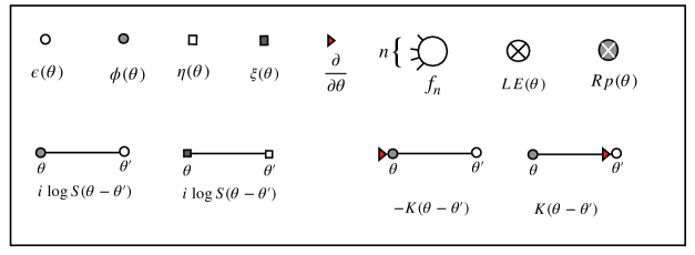
Figure 5: Feynman rules for the HS fields on a cylinder. The coefficients $f_{n}$ are depicted by white blobs with $n$ legs. The fields $\bm{\epsilon},{{\bm{\phi}}},\bm{\eta},\bm{\psi}$ are represented respectively by light and dark dots and squares. The derivative $\partial_{\theta}$ is symbolised by a red triangle pointing to the element at which the derivative is applied.

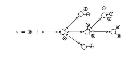
Figure 6: Feynman graph expansion for the pseudoenergy $\epsilon=\langle\bm{\epsilon}\rangle_{\text{cyl}}$

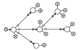
Figure 7: A typical Feynman graph contributing to the free energy

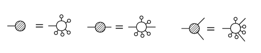
Figure 8: The dressed vertices $f_{1}[\epsilon],f_{2}[\epsilon],f_{3}[\epsilon]$.

The Feynman graph expansion can be defined for any classical background $\epsilon$. The corresponding Feynmann rules will be the same, with the vertices and the tadpoles replaced as

$$\begin{aligned} f_{n}\to f_{n}[\epsilon]\equiv&\sum_{k=0}^{\infty}f_{k+n}{\epsilon^{k}\over k!}=(-1)^{n-1}\text{Li}_{2-n}\left(-e^{-\epsilon}\right),\ \ n=1,2,...\end{aligned}$$ (A.5)

This relation between the old, ‘bare’, vertices and the new, ‘dressed’, ones is illustrated by fig. 8, where the dressed vertices are represented by hatched blobs. The first three vertices are

$$\begin{aligned} f_{1}[\epsilon]&=\log(1+e^{-\epsilon}),\ \ f_{2}[\epsilon]=-{1\over 1+e^{\epsilon}},\quad f_{3}[\epsilon]={1\over(1+e^{\epsilon})(1+e^{-\epsilon})}.\end{aligned}$$ (A.6)

If the background $\epsilon$ satisfies the classical equation (2.37), the diagram technique does not produce trees. Since the loops cancel, the free energy is given by a single graph

$$\begin{aligned} \mathcal{F}_{\text{cyl}}&=R\int{d\theta\over 2\pi}f_{1}[\epsilon(\theta)]\partial p(\theta)={\begin{picture}(5.0,0.0)(-4.0,5.0)\put(-3.5,3.5){\includegraphics[height=14.22636pt]{freeenergydressed}} \end{picture}}\hskip 14.51074pt.\end{aligned}$$ (A.7)

The pictorial form of the Ward identities (2.34) and (2.35) is

$$\begin{aligned} &{\begin{picture}(5.0,0.0)(-4.0,5.0)\put(-3.5,3.5){\includegraphics[height=14.22636pt]{WI1}} \end{picture}}\hskip 102.71446pt,\ \ \ \\ &{\begin{picture}(5.0,0.0)(-4.0,5.0)\put(-3.5,3.5){\includegraphics[height=14.22636pt]{WI2}} \end{picture}}\hskip 128.32176pt\end{aligned}$$ (A.8)

and that of the Leclair-Mussardo formula is

$$\begin{aligned} \ \langle{\mathcal{O}}\rangle_{R}&=\sum_{n=0}^{\infty}{(-1)^{n}\over n!}\int\prod_{j=1}^{n}{d\theta_{j}\over 2\pi}f_{2}[\epsilon(\theta_{j})]\ F^{c}_{2n}(\theta_{1},\dots,\theta_{n})\\ \\ &=\sum_{n=0}^{\infty}(-1)^{n}{\begin{picture}(5.0,0.0)(-4.0,5.0)\put(-3.5,-2.5){\includegraphics[height=54.06006pt]{LM.pdf}} \end{picture}}\hskip 34.42802pt.\end{aligned}$$ (A.9)

A.2 Feynman diagram technique for the torus

Let us again choose the fermionic TBA statistics, $\sigma=-1$. The interaction potential is expanded as

$$\begin{aligned} {\mathbf{F}}_{\text{tor}}=&\int_{\mathbb{R}}{d\theta\over 2\pi}\left[f_{1}[\bm{\epsilon}]\partial_{\theta}{{\bm{\phi}}}\,-f_{2}[\bm{\epsilon}]\bm{\eta}\partial_{\theta}\bm{\xi}\right]-\oint_{\mathcal{C}_{\mathbb{R}}}{d\theta\over 2\pi}f_{2}[-i{{\bm{\tilde{\phi}}}}]\left[f_{1}[{\bm{\tilde{\epsilon}}}]{\partial_{\theta}{{\bm{\tilde{\phi}}}}}-f_{2}[{\bm{\tilde{\epsilon}}}]{\bm{\tilde{\eta}}}\partial_{\theta}\bm{\tilde{\xi}}\right]\,\\ &=\sum_{n=0}^{\infty}\int_{\mathbb{R}}{d\theta\over 2\pi}\left(f_{n+1}\frac{\bm{\epsilon}^{n}}{n!}\partial_{\theta}{{\bm{\phi}}}-f_{n+2}\frac{\bm{\epsilon}^{n}}{n!}\bm{\eta}\partial_{\theta}\bm{\xi}\right)\\ &+\sum_{n,m=1}^{\infty}\oint_{\mathcal{C}_{\mathbb{R}}}{d\theta\over 2\pi}\left(-f_{m+1}f_{n+2}{{\bm{\tilde{\epsilon}}}^{m}\over m!}\ \partial_{\theta}{{\bm{\tilde{\phi}}}}{(-i{{\bm{\tilde{\phi}}}})^{n}\over n!}+f_{n+2}f_{m+2}{{\bm{\tilde{\epsilon}}}^{m}\over m!}{(-i{{\bm{\tilde{\phi}}}})^{n}\over n!}{\bm{\tilde{\eta}}}\partial_{\theta}\bm{\tilde{\xi}}\right)\end{aligned}$$ (A.10)

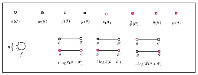
Figure 9: Feynman rules for the HS fields on a torus. The mirror-transformed fields are represented by the same symbols colored in magenta.

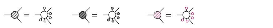
Figure 10: Dressed vertices for the torus.

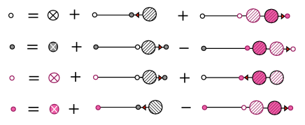
Figure 11: Pictorial form of the mean-field equations (4.23) for the classical values $\epsilon,\phi,\tilde{\epsilon},\tilde{\phi}$.

With the Feynman rules depicted in fig. 9, the interacting potential for the HS fields can be represented as

$$\begin{aligned} {\mathbf{F}}_{\text{cyl}}&=\sum_{n=0}^{\infty}{\begin{picture}(15.0,15.0)(-4.0,5.0)\put(-3.5,2.0){\includegraphics[height=22.76228pt]{int1.pdf}} \end{picture}}\hskip 0.0pt\ \ +\sum_{n=0}^{\infty}\ \ \ \ \ \ \ \ \ \ \ \ \ \begin{picture}(-15.0,-15.0)(9.0,5.0)\put(-3.5,2.0){\includegraphics[height=22.76228pt]{int2.pdf}} \end{picture}\hskip 48.36958pt\ +\sum_{m,n=0}^{\infty}\ \ \ \ \ \ \ \ \ \ \ \ \ \begin{picture}(-15.0,-15.0)(9.0,5.0)\put(-3.5,2.0){\includegraphics[height=22.76228pt]{intmn1.pdf}} \end{picture}\hskip 48.36958pt\ \ \ \ \ \ \ \ \ \ \ \ +\sum_{m,n=0}^{\infty}\ \ \ \ \ \ \ \ \ \ \ \ \ \begin{picture}(-15.0,-15.0)(9.0,5.0)\put(-3.5,2.0){\includegraphics[height=22.76228pt]{intmn2.pdf}} \end{picture}\hskip 48.36958pt\end{aligned}$$ (A.11)

The diagram expansion comprises diagrams with the structure of trees with arbitrary number of cycles. The sum over trees can be absorbed into the definition of the vertices if the Feynman rules are determined by the expansion around the mean field solution (4.23) .

References

- [1] A. Zamolodchikov, “Relativistic Factorized S Matrix in Two-Dimensional Space- Time with Isotopic O(n) Symmetry,” Pisma Zh. Eksp. Teor. Fiz. 26 (1977) 608–611.
- [2] E. Beth and G. E. Uhlenbeck, “The quantum theory of the non-ideal gas. II. Behaviour at low temperatures,” Physica 4 (1937), no. 10, 915–924.
- [3] R. Dashen, S.-k. Ma, and H. J. Bernstein, “-Matrix Formulation of Statistical Mechanics,” Phys. Rev. 187 (Nov, 1969) 345–370.
- [4] C. Yang and C. Yang, “Thermodynamics of a one-dimensional system of bosons with repulsive delta-function interaction,” Journ. Math. Phys. 10 (1969) 1115.
- [5] A. B. Zamolodchikov, “Thermodynamic Bethe Ansatz in relativistic models. Scaling three state Potts and Lee-Yang models,” Nucl. Phys. B342 (1990) 695–720.
- [6] A. B. Zamolodchikov, “From tricritical Ising to critical Ising by thermodynamic Bethe ansatz,” Nucl. Phys. B358 (1991) 524–546.
- [7] A. B. Zamolodchikov, “TBA equations for integrable perturbed coset models,” Nucl. Phys. B366 (1991) 122–134.
- [8] G. Mussardo, Statistical Field Theory. An Introduction to Exactly Solved Models in Statistical Physics An Introduction to Exactly Solved Models in Statistical Physics Statistical Field Theory An Introduction to Exactly Solved Models in Statistical Physics. Oxford University Press, Second Edition, 2020.
- [9] P. Dorey and R. Tateo, “Excited states by analytic continuation of TBA equations,” Nucl. Phys. B482 (1996) 639–659, hep-th/9607167.
- [10] C. Itzykson and J.-B. Zuber, “Two-dimensional conformal invariant theories on a torus,” Nuclear Physics B 275 (1986), no. 4, 580–616.
- [11] P. di Francesco, H. Saleur, and J. B. Zuber, “Relations between the Coulomb gas picture and conformal invariance of two-dimensional critical models,” Journal of Statistical Physics 49 (1987), no. 1, 57–79.
- [12] I. Kostov, “Free field representation of the coset models on the torus,” Nucl. Phys. B300 (1988) 559.
- [13] O. Foda and B. Nienhuis, “THE COULOMB GAS REPRESENTATION OF CRITICAL RSOS MODELS ON THE SPHERE AND THE TORUS,” Nucl. Phys. B324 (1989) 643.
- [14] H. Saleur and P. di Francesco, “Two-dimensional critical models on a torus,”. In *Poiana Brasov 1987, Proceedings, Conformal invariance and string theory* 63-87. (see Conference Index).
- [15] H. Saleur and C. Itzykson, “Two-dimensional field theories close to criticality,” Journal of Statistical Physics 48 (Aug, 1987) 449–475.
- [16] T. R. Klassen and E. Melzer, “The Thermodynamics of purely elastic scattering theories and conformal perturbation theory,” Nucl.Phys. B350 (1991) 635–689.
- [17] J. L. Jacobsen, Y. Jiang, and Y. Zhang, “Torus partition function of the six-vertex model from algebraic geometry,” 1812.00447.
- [18] J. Böhm, J. L. Jacobsen, Y. Jiang, and Y. Zhang, “Geometric Algebra and Algebraic Geometry of Loop and Potts Models,” 2202.02986.
- [19] Z. Bajnok, J. L. Jacobsen, Y. Jiang, R. I. Nepomechie, and Y. Zhang, “Cylinder partition function of the 6-vertex model from algebraic geometry,” JHEP 06 (2020) 169, 2002.09019.
- [20] I. Kostov, “Effective Quantum Field Theory for the Thermodynamical Bethe Ansatz,” Journal of High Energy Physics 2020 (2020), no. 2, 43.
- [21] A. M. Polyakov, “GAUGE FIELDS AND STRINGS,”. CHUR, SWITZERLAND: HARWOOD (1987) 301 P. (CONTEMPORARY CONCEPTS IN PHYSICS, 3).
- [22] M. Wadati, “Bosonic Formulation of the Bethe Ansatz Method,” Journal of the Physical Society of Japan 54 (1985), no. 10, 3727–3733, https://doi.org/10.1143/JPSJ.54.3727.
- [23] G. Mussardo and P. Simon, “Bosonic type S matrix, vacuum instability and CDD ambiguities,” Nucl. Phys. B 578 (2000) 527–551, hep-th/9903072.
- [24] L. Córdova, S. Negro, and F. I. Schaposnik Massolo, “Thermodynamic Bethe Ansatz past turning points: the (elliptic) sinh-Gordon model,” 2110.14666.
- [25] M. Gaudin, B. M. McCoy, and T. T. Wu, “Normalization sum for the Bethe’s hypothesis wave functions of the Heisenberg-Ising chain,” Phys. Rev. D 23 (Jan, 1981) 417–419.
- [26] I. Kostov, D. Serban, and D.-L. Vu, “TBA and tree expansion,” 2018. arXiv[hep-th]1805.02591.
- [27] I. Kostov, D. Serban, and D.-L. Vu, “Boundary TBA, trees and loops,” 1809.05705.
- [28] R. L. Stratonovich, “On a Method of Calculating Quantum Distribution Functions,” Soviet Physics Doklady 2 (July, 1957) 416.
- [29] J. Hubbard, “Calculation of Partition Functions,” Phys. Rev. Lett. 3 (Jul, 1959) 77–78.
- [30] A. Leclair and G. Mussardo, “Finite temperature correlation functions in integrable QFT,” Nucl. Phys. B552 (1999) 624–642, hep-th/9902075.
- [31] A. E. Ferdinand and M. E. Fisher, “Bounded and Inhomogeneous Ising Models. I. Specific-Heat Anomaly of a Finite Lattice,” Phys. Rev. 185 (Sep, 1969) 832–846.
- [32] N. V. Vdovichenko, “A calculation of the partition function for a plane dipole lattice,” Soviet Physics JETP 20 (1965), no. 2, 477–479.
- [33] H. A. Kramers and G. H. Wannier, “Statistics of the Two-Dimensional Ferromagnet. Part I,” Phys. Rev. 60 (Aug, 1941) 252–262.
- [34] T. Morita, “Partition function of a finite Ising model on a torus,” Journal of Physics A: Mathematical and General 19 (dec, 1986) L1191–L1196.
- [35] U. Wolff, “Ising model as Wilson-Majorana fermions,” Nuclear Physics B 955 (2020) 115061.
- [36] Z. Bajnok and F. Smirnov, “Diagonal finite volume matrix elements in the sinh-Gordon model,” 1903.06990.
- [37] J. Teschner, “On the spectrum of the Sinh-Gordon model in finite volume,” Nucl.Phys.B 799 (2008) 403–429, hep-th/0702214.
- [38] T. R. Klassen and E. Melzer, “Purely Elastic Scattering Theories and their Ultraviolet Limits,” Nucl.Phys. B338 (1990) 485–528.
- [39] S. N. Vergeles and V. M. Gryanik, “Two-Dimensional Quantum Field Theories Having Exact Solutions,” Sov. J. Nucl. Phys. 23 (1976) 704–709.
- [40] I. Arefyeva and V. Korepin, “Scattering in two-dimensional model with Lagrangian ,” Pis’ma v ZhetF 20 (1974) 680.
- [41] A. B. Zamolodchikov, “Mass scale in the sine-Gordon model and its reductions,” Int. J. Mod. Phys. A10 (1995) 1125–1150.
- [42] A. Arinshtein, V. Fateyev, and A. Zamolodchikov, “Quantum S-matrix of the (1 + 1)-dimensional Todd chain,” Physics Letters B 87 (1979), no. 4, 389–392.
- [43] A. B. Zamolodchikov, “On the thermodynamic Bethe ansatz equation in sinh-Gordon model,” J. Phys. A39 (2006) 12863–12887, hep-th/0005181.
- [44] C. Destri and H. D. Vega, “New exact results in Affine Toda field theories: Free energy and wave-function renormalizations,” Nuclear Physics B 358 (1991), no. 1, 251 – 294.
- [45] S. L. Lukyanov, “Finite temperature expectation values of local fields in the sinh-Gordon model,” Nucl. Phys. B612 (2001) 391–412, hep-th/0005027.
- [46] S. Negro and F. Smirnov, “On one-point functions for sinh-Gordon model at finite temperature,” Nucl.Phys. B875 (2013) 166–185, 1306.1476.