1 Introduction

Tunnelling in quantum field theory is a fascinating subject. In many respects, it differs substantially from the analogous phenomenon in ordinary quantum mechanics with a finite number of degrees of freedom, and deserves a special treatment. In a couple of famous papers [1, 2], S. Coleman and C. Callan have shown that the semi-classical approximation, in conjunction with path integral techniques, provides a suited context to deal with quantum tunnelling with infinite degrees of freedom. The first purpose of this work is to review both the semi-classical approximation in quantum mechanics and its extension to quantum field theory, as illustrated in Refs. [1, 2]. We will adopt a pedagogical attitude: special attention will be devoted to the derivation of the bounce formalism, the definition and calculation of functional determinants, and the role of renormalization. All steps in the derivation of these known results, some of which are omitted in the original literature, are carefully illustrated.

A remarkable feature of tunnelling in quantum field theory is that the transition from the false to the true vacuum does not take place between two spatially homogeneous field configurations, but rather through the formation of a bubble of true vacuum in a false-vacuum background. Such field configuration (the bounce) is therefore not spatially homogenous, and the gradient term in the potential energy gives a non-zero contribution to the full potential energy. This is different from the case of ordinary quantum mechanics, in which the gradient term is absent and the tunnelling rate does not depend on the physics beyond the potential barrier.

An important application of the formalism above is the study of the stability of the electroweak vacuum in the case of the standard model of electroweak interactions. The accurate measurements of the top quark and Higgs boson masses indicate that the electroweak vacuum, which determines the observed spectrum of physical particles, is not the absolute ground state of the electroweak theory. Extrapolating the Higgs effective potential at high energies, the electroweak minimum becomes metastable for Higgs field values around $10^{10}$ GeV. Many efforts have been devoted to establish whether the lifetime metastable vacuum of the standard model is sufficiently larger that the age of the Universe, and therefore compatible with observations, or else if physics beyond the standard model is needed in order to justify the observed electroweak spectrum.

The application of the formalism outlined in Refs. [1, 2] to the standard model is not straightforward. At the level of the classical Lagrangian, the electroweak vacuum corresponds to a true minimum of the scalar potential, and it is only upon the inclusion of quantum corrections that the instability occurs. Furthermore, the tunnelling rate calculation in the standard model including the first quantum corrections (originally addressed in Ref. [3]) is complicated by the presence of many degrees of freedom with different spin, and by the approximate scale invariance of the theory at high-energy scales, relevant for the tunnelling process in the standard model.

In the second part of this work, we will review several aspects of the calculation of the electroweak vacuum lifetime. In particular, we will carefully discuss the role of approximate scale invariance for the determination of the standard model bounce, which selects energy scales of order $10^{17}$ GeV. Since the latter is very close to the Planck scale, it is a legitimate question to ask whether gravitational effects can become relevant in this regime. After addressing the ultraviolet sensitivity of the standard model vacuum decay rate [4], we will take gravitational effects into account within the formalism of Coleman and De Luccia [5], arguing that as long as gravity can be treated as an effective field theory in a perturbative regime [6], the standard model calculation does not get drastically affected.

The review is organized as follows: in Sect. 2 we introduce the phenomenon of quantum tunnelling in quantum mechanics with some explicit examples. We then generalize this formalism to the case of quantum mechanics with many degrees of freedom, thus providing the tools required for dealing with tunnelling in quantum field theory, which is the main subject of Sect. 3. Sect. 4 is devoted to a review of effective potential methods, a necessary step in order to introduce the problem of the instability of the Higgs potential in the standard model. The calculation of the standard model vacuum decay rate is illustrated in Sect. 5, together with the construction on the so-called standard model phase diagram and the possible impact of non-standard physics. Sect. 6 is devoted to the study of gravitational corrections to the standard model vacuum decay rate.

Some technical issues are collected in the Appendices, mainly with the purpose of casting well-known results in the notations adopted in the text, for the ease of the reader. App. A.1 is a simple review of the semi-classical approximation in ordinary quantum mechanics, which is applied in the following App. A.2 to the calculation of the lowest-level energy splitting for a symmetric double-well potential. This is a simple exercise in quantum mechanics, which is included here for the purpose of comparison with the analogous calculation by path-integral methods presented in the text. Small differences between the two results are discussed. The Maupertuis principle is reviewed in App. A.3, while App. A.4 describes briefly Legendre transformations. App. A.5 contains a derivation of the Fubini-Lipatov bounce. In App. A.6 we describe the techniques employed to obtain bounce solutions by numerical methods. Finally, the derivation of the gravitational field equations for a scalar field minimally coupled to gravity is described in App. A.7.

2 Tunnelling in quantum mechanics

In this section we review the phenomenon of tunnelling through barriers due to quantum fluctuations. We will start from ordinary quantum mechanics in one space dimension, extend the results to the case of many degrees of freedom, and finally generalize to quantum field theory. We will follow closely the work by Coleman and collaborators [1, 2]. See also Ref. [7] for a comprehensive review.

2.1 Tunnelling in one dimension

Tunnelling is a typical phenomenon of quantum mechanics. The simplest example is the case of a beam of particles (or a wave packet) moving in one space dimension towards a potential energy barrier $U(x)$ whose maximum value is larger than the particle energy: in quantum mechanics the particles of the beam have a non-zero probability of being transmitted beyond the potential barrier, contrary to what happens in classical mechanics. The relevant quantity to be computed is the transmission coefficient, defined as the ratio between the transmitted flux and the incident flux.

If the potential barrier is sufficiently high and broad, the transmission coefficient is conveniently computed within the semi-classical or Wentzel-Kramers-Brillouin (WKB) approximation, which is reviewed in some detail in App. A.1. It turns out that, in the leading semi-classical approximation, the transmission coefficient $\cal T$ through a potential barrier is given by [8]

$${\cal T}=A_{T}e^{-B};\qquad B=\frac{2}{\hbar}\int_{a}^{b}|p(x)|dx=\frac{2}{\hbar}\int_{a}^{b}\sqrt{2m[U(x)-E]}dx,$$ (2.1)

where $E$ is the energy of the incident particles, and $a,b$ are the classical turning points, $U(a)=U(b)=E$. The overall factor $A_{T}$ is not fixed in the leading semi-classical approximation.

The result Eq. (2.1) can also be used to estimate the decay probability per unit time $\gamma$ of a metastable state, which is the case of interest to us. Indeed, if the barrier separates a local minimum of the potential energy from a deeper minimum, then the probability per unit time $\gamma$ that the particle, initially localized around the local minimum with energy $E_{0}$, the fundamental level of the local minimum, penetrates the barrier, is proportional to $\cal T$. The exact proportionality coefficient cannot be computed within the lowest-order semi-classical approximation. However, it must be proportional to the number $N$ of times the particle hits the barrier per unit time. Approximating the initial state as an oscillatory state with frequency $\omega=\frac{E_{0}}{\hbar}$, we have simply $N=\frac{\omega}{2\pi}=\frac{1}{t_{\rm cl}}$, where $t_{\rm cl}$ is the classical period of the oscillation. Hence [9]

$$\gamma\simeq\frac{\cal T}{t_{\rm cl}}\equiv Ae^{-B}.$$ (2.2)

It is customary to define a decay width

$$\Gamma=\hbar\gamma,$$ (2.3)

with the dimension of an energy, whose physical meaning will be clear in a moment.

Finally, we note that, if the particle has a probability per unit time $\gamma$ to escape from the local minimum, then the probability $P(t)$ to find it in the vicinity of the local minimum decreases in time according to

$$\frac{dP(t)}{dt}=-\gamma P(t),$$ (2.4)

which has the solution

$$P(t)=P(0)e^{-\gamma t}=P(0)e^{-\frac{\Gamma t}{\hbar}}.$$ (2.5)

This suggests that we may interpret the unstable state as an approximate stationary state with complex energy eigenvalue:

$$E=E_{0}-i\frac{\Gamma}{2},$$ (2.6)

so that the corresponding wave function evolves in time according to

$$\Psi(x,t)=\psi(x)e^{-i\frac{E_{0}t}{\hbar}}e^{-\frac{\Gamma t}{2\hbar}},$$ (2.7)

consistently with Eq. (2.5).

2.2 The double-well potential

A typical application of the semi-classical approximation method is the calculation of the splitting between the two lowest energy eigenvalues of a one-dimensional hamiltonian whose potential energy has two degenerate minima, such as the one sketched in the left panel of Fig. 1. The standard calculation can be found for example in Ref. [8], and it is reviewed in App. A.2.

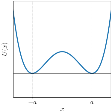
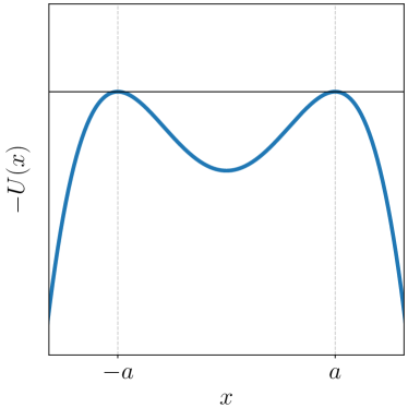
Figure 1: Left panel: double-well potential with two symmetric minima in $\pm a$. Right panel: the same potential after the change of sign.

For our present purposes, it will prove useful to obtain the result of App. A.2 in the context of the path integral formulation of quantum mechanics. In the case of one-dimensional ordinary quantum mechanics the path integral calculation turns out to be much more lengthy and complicated, but it has the advantage that it can be generalized to quantum field theory beyond the leading semi-classical approximation.

We will assume that the potential energy $U(x)$ has two degenerate minima at $x=\pm a$, and that $U^{\prime\prime}(\pm a)=m\omega^{2}$, where $m$ is the mass of the particle and $\omega$ a real constant. An explicit example of such a potential is

$$U(x)=\frac{m\omega^{2}}{8a^{2}}(x^{2}-a^{2})^{2}.$$ (2.8)

It will often be useful to refer to the specific example in Eq. (2.8), for which analytic calculations are possible. Our final result, however, applies to a more general class of one-dimensional potential energies with a symmetric double well. In particular, we will keep $U_{0}=U(\pm a)$ different from zero.

The first step is switching to imaginary time, $t=i\tau$. The Lagrange function reads

$$L(x,\dot{x})=-\frac{1}{2}m\dot{x}^{2}-U(x),$$ (2.9)

where $x$ is the position of the particle,

$$\dot{x}=\frac{dx(\tau)}{d\tau},$$ (2.10)

and the conjugate momentum to the coordinate $x$ is

$$p=\frac{\partial L(x,\dot{x})}{\partial\dot{x}}=-m\dot{x},$$ (2.11)

so that the Hamiltonian reads

$$H(x,p)=p\dot{x}-L(x,\dot{x})=-\frac{1}{2}m\dot{x}^{2}+U(x).$$ (2.12)

This is called the Euclidean Hamiltonian, because the Minkowski space with imaginary time has a Euclidean metric (this is a slight abuse of language: the Minkowski space-time is not relevant here, since we are in a non-relativistic context.)

We consider the probability amplitudes for the particle to start at $x=-a$ at $\tau=-\frac{T}{2}$ and end up at either $x=+a$ or $x=-a$ at $\tau=\frac{T}{2}$:

$$Z_{\pm}(T)=\langle\pm a|e^{-\frac{HT}{\hbar}}|-a\rangle,$$ (2.13)

where $|\pm a\rangle$ are position eigenstates with eigenvalues $\pm a$. Inserting a complete set $|n\rangle$ of energy eigenstates

$$H|n\rangle=E_{n}|n\rangle$$ (2.14)

we get

$$Z_{\pm}(T)=\sum_{n}e^{-\frac{E_{n}T}{\hbar}}\langle\pm a|n\rangle\langle n|-a\rangle.$$ (2.15)

If the potential barrier between the two minima is sufficiently high and broad, the two lowest levels $E_{1},E_{2}$ differ from the lowest level in the absence of tunnelling, $E_{0}=\frac{\hbar\omega}{2}+U_{0}$, by an amount which is much smaller than the separation of $E_{0}$ from higher levels, of order $\hbar\omega$. Hence, in the large-$T$ limit, the sum in Eq. (2.15) is dominated by the two lowest eigenstates:

$$Z_{-}(T) =e^{-\frac{E_{1}T}{\hbar}}\langle-a|1\rangle\langle 1|-a\rangle+e^{-\frac{E_{2}T}{\hbar}}\langle-a|2\rangle\langle 2|-a\rangle$$ (2.16)

$$Z_{+}(T) =e^{-\frac{E_{1}T}{\hbar}}\langle+a|1\rangle\langle 1|-a\rangle+e^{-\frac{E_{2}T}{\hbar}}\langle+a|2\rangle\langle 2|-a\rangle,$$ (2.17)

up to terms that vanish more rapidly as $T\to\infty$. Furthermore, the wave functions of states $|1\rangle$ and $|2\rangle$ in the position representation are even and odd, respectively; thus

$$\langle+a|1\rangle=\langle-a|1\rangle;\quad\langle+a|2\rangle=-\langle-a|2\rangle.$$ (2.18)

Finally,

$$|\langle 1|+a\rangle|^{2}=|\langle 2|+a\rangle|^{2}.$$ (2.19)

As a consequence,

$$Z_{-}(T) =|\langle 1|a\rangle|^{2}\left(e^{-\frac{E_{1}T}{\hbar}}+e^{-\frac{E_{2}T}{\hbar}}\right)$$ (2.20)

$$Z_{+}(T) =|\langle 1|a\rangle|^{2}\left(e^{-\frac{E_{1}T}{\hbar}}-e^{-\frac{E_{2}T}{\hbar}}\right)$$ (2.21)

and therefore, for large $T$,

$$\frac{Z_{-}(T)-Z_{+}(T)}{Z_{-}(T)+Z_{+}(T)}=e^{-\frac{(E_{2}-E_{1})T}{\hbar}},$$ (2.22)

or

$$E_{2}-E_{1}=-\hbar\lim_{T\to+\infty}\frac{1}{T}\log\frac{Z_{-}(T)-Z_{+}(T)}{Z_{-}(T)+Z_{+}(T)}.$$ (2.23)

Eq. (2.23) allows us to compute the energy splitting between the two lowest energy levels, provided the amplitudes $Z_{\pm}(T)$ can be computed in an independent way.

The path integral formalism provides such an independent calculation. Indeed, by standard path integral arguments it can be shown that

$$Z_{\pm}(T)=\int[dx]\,e^{-\frac{S[x]}{\hbar}},$$ (2.24)

where $[dx]$ is a functional measure, to be defined accurately below, over all paths $x(\tau)$ with

$$x\left(-\frac{T}{2}\right)=-a;\qquad x\left(\frac{T}{2}\right)=\pm a,$$ (2.25)

and $S[x]$ is the Euclidean action of the path:

$$S[x]=-\int_{-\frac{T}{2}}^{\frac{T}{2}}d\tau\,L(x,\dot{x})=\int_{-\frac{T}{2}}^{\frac{T}{2}}d\tau\,\left[\frac{1}{2}m\dot{x}^{2}+U(x)\right].$$ (2.26)

Let us now assume that $S[x]$ has a stationary point, i.e. a path $\overline{x}(\tau)$ such that $S[\overline{x}]$ is finite and stationary upon deformations around $\overline{x}(\tau)$. In this case, the path integral in Eq. (2.24) can be computed by means of a generalization of the saddle-point approximation technique. This is motivated by the observation that the exponent in the integrand of Eq. (2.24) is weighted by a factor of $\frac{1}{\hbar}$, which is large in the semi-classical limit $\hbar\to 0$; the contributions to the integral from field configurations far from the minimum configurations are therefore exponentially suppressed in this limit.

In the leading saddle-point approximation, the functional integral is simply given by the value of the integrand computed in correspondence of the path which minimizes $S[x]$, that is, a solution of the classical equations of motions. The next-to-leading correction involves a calculation of the first non-trivial fluctuations of the exponent around the stationary point; for this reason we need the idea of a functional Taylor expansion, and therefore of functional differentiation. Functional derivatives are defined by

$$\frac{\delta x(\tau)}{\delta x(\tau^{\prime})}=\delta(\tau-\tau^{\prime}),$$ (2.27)

together with the usual rules of differentiations of sums and products of ordinary functions. We find

$$\frac{\delta S[x]}{\delta x(\tau)} =\int_{-\frac{T}{2}}^{\frac{T}{2}}d\tau^{\prime}\,\left[m\frac{dx}{d\tau^{\prime}}\frac{d}{d\tau^{\prime}}\delta(\tau-\tau^{\prime})+U^{\prime}(x)\delta(\tau-\tau^{\prime})\right]$$

$$=-m\ddot{x}(\tau)+U^{\prime}(x(\tau)),$$ (2.28)

where we have used

$$\int_{-\frac{T}{2}}^{\frac{T}{2}}d\tau\,f(\tau)\frac{d^{n}}{d\tau^{n}}\delta(\tau)=(-1)^{n}\frac{d^{n}f(0)}{d\tau^{n}}.$$ (2.29)

The second functional derivative of the action is given by

$$\frac{\delta^{2}S[x]}{\delta x(\tau^{\prime})\delta x(\tau)} =-m\frac{d^{2}}{d\tau^{2}}\delta(\tau-\tau^{\prime})+U^{\prime\prime}(x)\delta(\tau-\tau^{\prime})$$

$$=\left[-m\frac{d^{2}}{d\tau^{2}}+U^{\prime\prime}(x)\right]\delta(\tau-\tau^{\prime})\equiv S^{\prime\prime}[x]\delta(\tau-\tau^{\prime}).$$ (2.30)

We now take the functional Taylor expansion of $S[x]$ in the vicinity of a solution $\overline{x}(\tau)$ of the classical equation of motion:

$$\left.\frac{\delta S[x]}{\delta x(\tau)}\right|_{x=\overline{x}}=-m\ddot{\overline{x}}+U^{\prime}(\overline{x})=0$$ (2.31)

with the boundary conditions Eq. (2.25). We find

$$S[x] =S[\overline{x}]+\frac{1}{2}\int_{-\frac{T}{2}}^{\frac{T}{2}}d\tau\,\int_{-\frac{T}{2}}^{\frac{T}{2}}d\tau^{\prime}\,\delta x(\tau)S^{\prime\prime}[\overline{x}]\delta(\tau-\tau^{\prime})\delta x(\tau^{\prime})+O((\delta x)^{3})$$

$$=S[\overline{x}]+\frac{1}{2}\int_{-\frac{T}{2}}^{\frac{T}{2}}d\tau\,\delta x(\tau)S^{\prime\prime}[\overline{x}]\delta x(\tau)+O((\delta x)^{3})$$ (2.32)

where $\delta x(\tau)=x(\tau)-\overline{x}(\tau)$.

As in the case of a finite-dimensional gaussian integral, it is convenient to introduce a set of eigenfunctions of $S^{\prime\prime}[\overline{x}]$:

$$S^{\prime\prime}[\overline{x}]\psi_{n}(\tau)=\left[-m\frac{d^{2}}{d\tau^{2}}+U^{\prime\prime}(\overline{x})\right]\psi_{n}(\tau)=\lambda_{n}\psi_{n}(\tau),$$ (2.33)

which can be taken to be orthogonal and normalized:

$$\int_{-\frac{T}{2}}^{\frac{T}{2}}d\tau\,\psi_{n}(\tau)\psi_{m}(\tau)=\delta_{nm};\qquad\psi_{n}\left(\pm\frac{T}{2}\right)=0.$$ (2.34)

A generic path can be parametrized as

$$x(\tau)=\overline{x}(\tau)+\sum_{n}c_{n}\psi_{n}(\tau).$$ (2.35)

The integration over all possible paths is therefore identified with an integration over all possible values of the coefficients $c_{n}$. This suggests that the functional measure $[dx]$ be defined by

$$[dx]=N\prod_{n}\frac{dc_{n}}{\sqrt{2\pi\hbar}}.$$ (2.36)

The factors of $\frac{1}{\sqrt{2\pi\hbar}}$ and the overall factor $N$ have been introduced for later convenience. The expansion of $S[x]$ around $\overline{x}$ to second order, Eq. (2.32), takes the form

$$S[x]=S[\overline{x}]+\frac{1}{2}\sum_{n}\lambda_{n}c_{n}^{2}+O(c_{n}^{3}),$$ (2.37)

and the path integral Eq. (2.24) can be computed as an infinite product of gaussian integrals:

$$Z_{\pm}(T) =Ne^{-\frac{S[\overline{x}]}{\hbar}}\prod_{n}\frac{1}{\sqrt{2\pi\hbar}}\int_{-\infty}^{+\infty}dc_{n}\,e^{-\frac{1}{2\hbar}\lambda_{n}c_{n}^{2}}$$

$$=Ne^{-\frac{S[\overline{x}]}{\hbar}}\prod_{n}\frac{1}{\sqrt{\lambda_{n}}}$$ (2.38)

(the dependence of the r.h.s. of Eq. (2.38) on the $\pm$ sign in the l.h.s. is hidden in the boundary values of the stationary path $\overline{x}$ and in the eigenvalues $\lambda_{n}$.) We now formally define the determinant of an operator on a space of functions, denoted by the symbol Det, as the product of its eigenvalues:

$$\mbox{Det}\,S^{\prime\prime}[\overline{x}]=\prod_{n}\lambda_{n},$$ (2.39)

so that, at least formally,

$$Z_{\pm}(T)=\frac{N}{\sqrt{\mbox{Det}\,S^{\prime\prime}[\overline{x}]}}e^{-\frac{S[\overline{x}]}{\hbar}}.$$ (2.40)

A few comments are in order.

• The result Eq. (2.40) holds provided all eigenvalues $\lambda_{n}$ are strictly positive. We will see that this is not the case in some relevant situations, including the present one. We will show later in this section how to deal with this difficulty.

• The determinant in Eq. (2.40) is divergent, since it is the infinite product of positive and growing numbers. This infinity is usually absorbed by a suitable definition of the constant $N$ in the functional integration measure. However, we shall not need an explicit expression of $N$, because it cancels in the calculation of the splitting between the two lowest energy eigenvalues.

• If there are more paths which minimize the Euclidean action, $x_{n}(\tau),n=0,1,\ldots$, the path integral receives one contribution Eq. (2.40) from each of them:

  $$Z_{\pm}(T)=N\sum_{n}\frac{1}{\sqrt{\mbox{Det}\,S^{\prime\prime}[\overline{x}_{n}]}}e^{-\frac{S[\overline{x}_{n}]}{\hbar}}.$$ (2.41)

In order to complete the calculation of the energy splitting $E_{2}-E_{1}$ from Eq. (2.23), we must therefore i) find all the minimum paths for the Euclidean action, and ii) learn how to compute determinants of operators on spaces of functions. Both steps are not trivial, and we will carefully go through the details.

2.2.1 Stationary paths

We first address the problem of finding all paths $\overline{x}(\tau)$ which minimize the Euclidean action. In order to help intuition, it is useful to view Eq. (2.31) as the equation of motion of a particle under the effect of the potential $-U(x)$ in real time (see the right panel of Fig. 1).

As far as $Z_{-}(T)$ is concerned, for which $x(T/2)=-a$, one solution is obviously

$$\overline{x}(\tau)=x_{0}(\tau)=-a$$ (2.42)

for all times $\tau$. We have

$$S[x_{0}]=U_{0}T;\qquad S^{\prime\prime}[x_{0}]=-m\frac{d^{2}}{d\tau^{2}}+m\omega^{2},$$ (2.43)

and the corresponding contribution to the path integral is

$$I[x_{0}]=\frac{N}{\sqrt{\mbox{Det}\,S^{\prime\prime}[x_{0}]}}e^{-\frac{S[x_{0}]}{\hbar}}.$$ (2.44)

The action $S[x_{0}]$ vanishes if we set the zero of the potential at $x=\pm a$, as in the case of Eq. (2.8). This is the choice adopted in Fig. 1 and in App. A.2. For the time being we keep however $U_{0}\neq 0$ for greater generality. Note that in this case $S[x_{0}]=U_{0}T$ is only finite for finite $T$.

In the case $x(T/2)=+a$, the particle starts from $x=-a$ at time $\tau=-T/2$ with zero velocity, and reaches $x=a$ at time $\tau=T/2$. This solution, which we will denote by $x_{1}(\tau)$, is usually called an instanton. The explicit form of $x_{1}(\tau)$ depends on the shape of the potential energy $U(x)$, but its main features follow from general considerations.

1. Because $U(x)$ is an even function, and the equation of motion is time-reversal invariant, we have $x_{1}(-\tau)=-x_{1}(\tau)$, and therefore $x_{1}(0)=0$.

2. From energy conservation,

   $$-\frac{1}{2}m\dot{x}_{1}^{2}+U(x_{1})=U_{0}$$ (2.45)

   we get

   $$\frac{dx_{1}(\tau)}{d\tau}=\sqrt{\frac{2[U(x_{1})-U_{0}]}{m}},$$ (2.46)

   where we have selected the positive sign because $x_{1}(\tau)$ is an increasing function of $\tau$. Eq. (2.46) implies that the particle spends most of the time close to either the initial position $x=-a$ or the final position $x=a$; the transition between these two values occurs within a short time interval of order $1/\omega$ (the instanton size) around $\tau=0$ (the instanton center).

3. When $T\to+\infty$, the instanton center can be located anywhere; hence, in this limit we must consider all solutions $x_{1}(\tau-\tau_{1})$ with $-\frac{T}{2}<\tau_{1}<\frac{T}{2}$. The one-instanton contribution is obtained by summing over all possible locations of the instanton center, i.e. by integrating over $\tau_{1}$ in this range:

   $$I[x_{1}]=\int_{-T/2}^{T/2}d\tau_{1}\,\frac{N}{\sqrt{\mbox{Det}\,S^{\prime\prime}[x_{1}]}}e^{-\frac{S[x_{1}]}{\hbar}}=\frac{N}{\sqrt{\mbox{Det}\,S^{\prime\prime}[x_{1}]}}Te^{-\frac{S[x_{1}]}{\hbar}}.$$ (2.47)

4. Using again Eq. (2.45), we find that the instanton action $S[x_{1}]$ can be expressed either in terms of the potential energy:

   $$S[x_{1}] =\int_{-T/2}^{T/2}d\tau\,2U(x_{1})-U_{0}T$$

   $$=\int_{-T/2}^{T/2}d\tau\,2[U(x_{1})-U_{0}]+U_{0}T$$

   $$=\int_{-a}^{a}dx\,\sqrt{2m[U(x)-U_{0}]}+S[x_{0}],$$ (2.48)

   or in terms of the kinetic energy:

   $$S[x_{1}]=\int_{-T/2}^{T/2}d\tau\,m\dot{x}_{1}^{2}+S[x_{0}].$$ (2.49)

   Both expressions will prove useful. Note that $S[x_{0}]$ (and therefore $S[x_{1}]$) is only finite for finite values of $T$, while the difference $S[x_{1}]-S[x_{0}]$ is finite even in the limit $T\to+\infty$.

We can check the above features of the instanton solution in the case of the potential Eq. (2.8). In this case, Eq. (2.46) can be integrated analytically:

$$x_{1}(\tau)=a\frac{e^{\omega\tau}-1}{e^{\omega\tau}+1}.$$ (2.50)

In this explicit example, $x_{1}(\tau)$ is close $\pm a$ for $|\tau|$ larger than a few times $\frac{1}{\omega}$; indeed $x_{1}(\pm 4/\omega)\simeq\pm 0.96\,a$. Hence, as anticipated, $x_{1}(\tau)$ differs sizeably from $\pm a$ only in an interval $-\delta<\tau<\delta$, with $\delta$ of order a few times $\omega^{-1}$. Furthermore, the instanton action can be computed analytically in this case. Using Eq. (2.48) and $S[x_{0}]=0$ we find

$$S[x_{1}]=\frac{m\omega}{2a}\int_{-a}^{a}dx\,(a^{2}-x^{2})=\frac{2ma^{2}\omega}{3}.$$ (2.51)

As anticipated, in the limit $T\to\infty$ the operator $S^{\prime\prime}[x_{1}]$ has a zero mode, that is, an eigenfunction with zero eigenvalue:

$$\psi_{0}(\tau)=C\frac{dx_{1}(\tau)}{d\tau},$$ (2.52)

where

$$C=\left[\int_{-\frac{T}{2}}^{\frac{T}{2}}d\tau\,\left|\frac{dx_{1}(\tau)}{d\tau}\right|^{2}\right]^{-\frac{1}{2}}=\sqrt{\frac{m}{S[x_{1}]-S[x_{0}]}}$$ (2.53)

by Eq. (2.49). Indeed,

$$\left[-m\frac{d^{2}}{d\tau^{2}}+U^{\prime\prime}(x_{1})\right]\frac{dx_{1}}{d\tau}=\frac{d}{d\tau}\left[-m\ddot{x}_{1}+U^{\prime}(x_{1})\right]=0$$ (2.54)

by the equation of motion. The presence of a zero mode implies that the integration over the corresponding coefficient $c_{0}$ leads to an infinity. Luckily, we do not need to perform this integration, because an infinitesimal change in $c_{0}$ is equivalent to an infinitesimal shift in the instanton center $\tau_{1}$:

$$\frac{dx(\tau)}{dc_{0}} =\psi_{0}(\tau)=\sqrt{\frac{m}{S[x_{1}]-S[x_{0}]}}\frac{dx_{1}}{d\tau}$$ (2.55)

$$\frac{dx(\tau)}{d\tau_{1}} =\frac{dx_{1}}{d\tau_{1}}=-\frac{dx_{1}}{d\tau},$$ (2.56)

or equivalently

$$\frac{dc_{0}}{\sqrt{2\pi\hbar}}=-\sqrt{\frac{S[x_{1}]-S[x_{0}]}{2\pi\hbar m}}d\tau_{1}.$$ (2.57)

Since we have already performed an integration over the instanton center $\tau_{1}$, we may simply omit the integration over $c_{0}$, which amounts to omitting the zero eigenvalue in the determinant, and multiply the result with the jacobain factor $\sqrt{\frac{S[x_{1}]-S[x_{0}]}{2\pi\hbar m}}$:

$$I[x_{1}]=\frac{N}{\sqrt{\mbox{Det}\,^{\prime}S^{\prime\prime}[x_{1}]}}\sqrt{\frac{S[x_{1}]-S[x_{0}]}{2\pi\hbar m}}Te^{-\frac{S[x_{1}]}{\hbar}}=I[x_{0}]KTe^{-\frac{S[x_{1}]-S[x_{0}]}{\hbar}}$$ (2.58)

where $I[x_{0}]$ is given in Eq. (2.44), we have defined

$$K=\sqrt{\frac{S[x_{1}]-S[x_{0}]}{2\pi\hbar m}}\sqrt{\frac{\mbox{Det}\,S^{\prime\prime}[x_{0}]}{\mbox{Det}\,^{\prime}S^{\prime\prime}[x_{1}]}}$$ (2.59)

and $\mbox{Det}\,^{\prime}$ stands for a determinant with the zero eigenvalue removed.

More approximate solutions of the equation of motion can be built out of the following observation. Given an instanton solution $x_{1}(\tau)$, then, by time reversal invariance,

$$x_{1}(-\tau)=-x_{1}(\tau)$$ (2.60)

is also a solution, with boundary conditions interchanged, and the same action as the instanton. This is called an anti-instanton. It follows that any sequence of an even [odd] number $n$ of alternate instanton and anti-instanton solutions contributes to the saddle-point estimate of $Z_{-}(T)$ [$Z_{+}(T)$]. We denote these solutions by $x_{n}(\tau)$.

In order to compute $S[x_{n}]$ we observe that, as in the single-instanton case, we may use energy conservation to obtain

$$S[x_{n}]=\int_{-T/2}^{T/2}d\tau\,m\dot{x}_{n}^{2}+S[x_{0}].$$ (2.61)

The function $x_{n}(\tau)$ is approximately equal to $\pm a$ almost everywhere in time, except for $n$ small intervals, of order $1/\omega$ in size, where it behaves as the single instanton or anti-instanton solutions. We may therefore approximate it by

$$x_{n}(\tau)\simeq x_{0}+\sum_{k=1}^{n}(-1)^{k+1}\left[x_{1}(\tau-\tau_{k})-x_{0}\right],$$ (2.62)

which gives

$$\dot{x}_{n}^{2}=\left[\sum_{k=1}^{n}(-1)^{k+1}\dot{x}_{1}(\tau-\tau_{k})\right]^{2}\simeq\sum_{k=1}^{n}\dot{x}^{2}_{1}(\tau-\tau_{k}),$$ (2.63)

where in the last step we have used the fact that $x_{1}(\tau-\tau_{k})$ is approximately constant for $\tau$ far from $\tau_{k}$. Hence, in the large-$T$ limit,

$$S[x_{n}]=n\left(S[x_{1}]-S[x_{0}]\right)+S[x_{0}],$$ (2.64)

and

$$I[x_{n}]=e^{-\frac{S[x_{0}]}{\hbar}}\left(e^{-\frac{S[x_{1}]-S[x_{0}]}{\hbar}}\right)^{n}\int[dx]\,\exp\left[-\frac{1}{2}\int_{-T/2}^{T/2}d\tau\,x(\tau)S^{\prime\prime}[x_{n}]x(\tau)\right].$$ (2.65)

In order to compute the functional integral, we observe that $S^{\prime\prime}[x_{n}]$ is approximately given by

$$S^{\prime\prime}[x_{n}]\simeq\left\{\begin{array}[]{ll}S^{\prime\prime}[x_{1}(\tau-\tau_{k})]&\tau_{k}-\delta<\tau<\tau_{k}+\delta\\ S^{\prime\prime}[x_{0}]&{\rm elsewhere}\end{array}\right.$$ (2.66)

where $k=1,\ldots,n$ and $\delta\sim\omega^{-1}$. This is a consequence of the fact that $x_{n}(\tau)$ is a multi-instanton solution in which the different instantons and anti-instantons are well separated from each other (this is usually called a dilute instanton gas; the validity of this assumption must be verified, which we will do in a moment.)

Let us now denote by $[dx]_{k}$ the functional integration measure over paths $x(\tau)$ that are sizably different from zero only in the range $\tau_{k}-\delta<\tau<\tau_{k}+\delta$, where $\tau_{k},k=1,\ldots,n$ are the centers of the $n$ instantons and anti-instantons. Using the approximation Eq. (2.66) we obtain

$$\int[dx]\,\exp\left[-\frac{1}{2}\int_{-T/2}^{T/2}d\tau\,x(\tau)S^{\prime\prime}[x_{n}]x(\tau)\right]$$

$$\qquad\qquad\simeq\int[dx]\,\exp\left[-\frac{1}{2}\int_{-T/2}^{T/2}d\tau\,x(\tau)S^{\prime\prime}[x_{0}]x(\tau)\right]$$

$$\qquad\qquad\times\prod_{k=1}^{n}\frac{\int[dx]_{k}\,\exp\left[-\frac{1}{2}\int_{-T/2}^{T/2}d\tau\,x(\tau)S^{\prime\prime}[x_{1}(\tau-\tau_{k})]x(\tau)\right]}{\int[dx]_{k}\,\exp\left[-\frac{1}{2}\int_{-T/2}^{T/2}d\tau\,x(\tau)S^{\prime\prime}[x_{0}])]x(\tau)\right]}.$$ (2.67)

The ratio under the product sign is in fact independent of $k$. Hence

$$\prod_{k=1}^{n}\frac{\int[dx]_{k}\,\exp\left[-\frac{1}{2}\int_{-T/2}^{T/2}d\tau\,x(\tau)S^{\prime\prime}[x_{1}(\tau-\tau_{k})]x(\tau)\right]}{\int[dx]_{k}\,\exp\left[-\frac{1}{2}\int_{-T/2}^{T/2}d\tau\,x(\tau)S^{\prime\prime}[x_{0}]x(\tau)\right]}$$

$$=\left[\frac{\int[dx]_{k}\,\exp\left[-\frac{1}{2}\int_{-T/2}^{T/2}d\tau\,x(\tau)S^{\prime\prime}[x_{1}(\tau-\tau_{k})]x(\tau)\right]}{\int[dx]_{k}\,\exp\left[-\frac{1}{2}\int_{-T/2}^{T/2}d\tau\,x(\tau)S^{\prime\prime}[x_{0}]x(\tau)\right]}\right]^{n}$$

$$=\left[\frac{\int[dx]\,\exp\left[-\frac{1}{2}\int_{-T/2}^{T/2}d\tau\,x(\tau)S^{\prime\prime}[x_{1}(\tau-\tau_{k})]x(\tau)\right]}{\int[dx]\,\exp\left[-\frac{1}{2}\int_{-T/2}^{T/2}d\tau\,x(\tau)S^{\prime\prime}[x_{0}]x(\tau)\right]}\right]^{n}$$ (2.68)

In the last step the functional integrals have been extended to all paths, not restricted by the condition of being different from zero only around $\tau_{k}$. This is allowed in the ratio, because $S^{\prime\prime}[x_{1}(\tau-\tau_{k})]$ and $S^{\prime\prime}[x_{0}]$ essentially coincide for $\tau$ not too close to $\tau_{k}$. Hence, leaving aside for the moment the problem of the zero mode of $S^{\prime\prime}[x_{1}]$, we find

$$\int[dx]\,\exp\left[-\frac{1}{2}\int_{-T/2}^{T/2}d\tau\,x(\tau)S^{\prime\prime}[x_{n}]x(\tau)\right]\simeq\frac{N}{\sqrt{\mbox{Det}\,S^{\prime\prime}[x_{0}]}}\left[\sqrt{\frac{\mbox{Det}\,S^{\prime\prime}[x_{0}]}{\mbox{Det}\,S^{\prime\prime}[x_{1}]}}\right]^{n}.$$ (2.69)

To complete the calculation of the $n$-instanton contribution, we must remove the zero eigenvalue from each factor of ${\rm det\,}S^{\prime\prime}[x_{1}]$, include $n$ jacobian factors

$$\sqrt{\frac{S[x_{1}]-S[x_{0}]}{2\pi\hbar m}}$$ (2.70)

and integrate over all possible locations $\tau_{1},\ldots,\tau_{n}$ of the instanton centers. This yields a factor of

$$\left[\sqrt{\frac{S[x_{1}]-S[x_{0}]}{2\pi\hbar m}}\right]^{n}\int_{-T/2}^{T/2}d\tau_{1}\int_{\tau_{1}}^{T/2}d\tau_{2}\ldots\int_{\tau_{n-1}}^{T/2}d\tau_{n}=\left[\sqrt{\frac{S[x_{1}]-S[x_{0}]}{2\pi\hbar m}}\right]^{n}\frac{T^{n}}{n!}.$$ (2.71)

So finally

$$I[x_{n}] =\frac{N}{\sqrt{\mbox{Det}\,S^{\prime\prime}[x_{0}]}}\frac{K^{n}T^{n}}{n!}e^{-\frac{n(S[x_{1}]-S[x_{0}])}{\hbar}}e^{-\frac{S[x_{0}]}{\hbar}}=I[x_{0}]\frac{1}{n!}\left[KTe^{-\frac{S[x_{1}]-S[x_{0}]}{\hbar}}\right]^{n}$$ (2.72)

with $K$ defined in Eq. (2.59). Note that our previous results Eqs. (2.44,2.58) are recovered for $n=0,1$ respectively.

We are now in a position to check the validity of the dilute instanton gas assumption. When all contributions $I[x_{n}]$ are summed up, the dominant contribution to the sum comes from values of $n$ for which

$$\frac{1}{n!}\left[KTe^{-\frac{S[x_{1}]-S[x_{0}]}{\hbar}}\right]^{n}\sim\frac{1}{(n-1)!}\left[KTe^{-\frac{S[x_{1}]-S[x_{0}]}{\hbar}}\right]^{n-1}$$ (2.73)

or

$$\frac{n}{T}\sim Ke^{-\frac{S[x_{1}]-S[x_{0}]}{\hbar}}.$$ (2.74)

We see that the instanton density $\frac{n}{T}$ for the relevant contributions is exponentially suppressed, as long as $S[x_{1}]-S[x_{0}]\gg\hbar$, which is the condition of validity of the semi-classical approximation (we will be able to check this statement in the explicit example of Eq. (2.8) after computing $K$.) This is an a posteriori confirmation of the reliability of our assumption that instantons and anti-instantons are well separated from each other in the relevant multi-instanton configurations.

2.2.2 Functional determinants

We now turn to the calculation of the ratio

$$\frac{\mbox{Det}\,S^{\prime\prime}[x_{0}]}{\mbox{Det}\,^{\prime}S^{\prime\prime}[x_{1}]}$$ (2.75)

which appears in the definition of $K$, Eq. (2.59). The procedure is illustrated in Ref. [10]; we will reproduce here the argument presented there, including some details which are omitted in Ref. [10]. We first show how to compute the ratio

$$\frac{\mbox{Det}\,O_{1}}{\mbox{Det}\,O_{2}},$$ (2.76)

where

$$O_{i}=-m\frac{d^{2}}{d\tau^{2}}+W_{i}(\tau);\qquad i=1,2$$ (2.77)

and $W_{i}(\tau)$ are arbitrary functions of $\tau$ in the range $-T/2\leq\tau\leq T/2$. Then, we remove the contribution of the minimum eigenvalue, which is different from zero as long as $T$ is kept finite, from the denominator of Eq. (2.76). Finally, we take the limit $T\to+\infty$.

Let us consider solutions $\phi^{(i)}_{\lambda}(\tau)$ of the Cauchy problem

$$O_{i}\phi^{(i)}_{\lambda}(\tau)=\lambda\phi^{(i)}_{\lambda}(\tau)$$ (2.78)

$$\phi^{(i)}_{\lambda}\left(-\frac{T}{2}\right)=0$$ (2.79)

$$\dot{\phi}^{(i)}_{\lambda}\left(-\frac{T}{2}\right)=1.$$ (2.80)

The important point here is that the function $\phi^{(i)}_{\lambda}(\tau)$, which certainly exists, because it is the unique solution to the Cauchy problem Eqs. (2.78, 2.79, 2.80), is not necessarily an eigenvector of $O_{i}$, because $\phi^{(i)}_{\lambda}(T/2)$ is in general different from zero. Also note that $\phi^{(i)}_{\lambda}(\tau)$ is not, in general, normalized to one.

We now define

$$F(\lambda)=\frac{\mbox{Det}\,(O_{1}-\lambda)}{\mbox{Det}\,(O_{2}-\lambda)};\qquad G(\lambda)=\frac{\phi^{(1)}_{\lambda}\left(\frac{T}{2}\right)}{\phi^{(2)}_{\lambda}\left(\frac{T}{2}\right)}.$$ (2.81)

The function $F(\lambda)$ has a simple zero whenever $\lambda$ is an eigenvalue $\lambda_{n}^{(1)}$ of $O_{1}$, and a simple pole whenever $\lambda$ is an eigenvalue $\lambda_{n}^{(2)}$ of $O_{2}$. The function $G(\lambda)$ has exactly the same poles and zeros. By Liouville’s theorem, the ratio $\frac{F(\lambda)}{G(\lambda)}$ is therefore a constant. Since both $F(\lambda)$ and $G(\lambda)$ tend to 1 as $\lambda\to\infty$ in any direction except the real axis, where both functions have simple poles, the constant is equal to one. Hence

$$F(\lambda)=G(\lambda)$$ (2.82)

in the whole complex plane $\lambda$. In particular, for $\lambda\to 0$,

$$\frac{\mbox{Det}\,O_{1}}{\mbox{Det}\,O_{2}}=\frac{\phi^{(1)}_{0}\left(\frac{T}{2}\right)}{\phi^{(2)}_{0}\left(\frac{T}{2}\right)},$$ (2.83)

which is the desired result.

We are interested in the case

$$O_{1}=S^{\prime\prime}[x_{0}]=-m\frac{d^{2}}{d\tau^{2}}+m\omega^{2}\qquad O_{2}=S^{\prime\prime}[x_{1}]=-m\frac{d^{2}}{d\tau^{2}}+U(x_{1}).$$ (2.84)

We need the solutions of the Cauchy problems

$$\left(-m\frac{d^{2}}{d\tau^{2}}+m\omega^{2}\right)\phi_{0}(\tau)=0;\qquad\phi_{0}\left(-\frac{T}{2}\right)=0;\qquad\dot{\phi}_{0}\left(-\frac{T}{2}\right)=1$$ (2.85)

$$\left(-m\frac{d^{2}}{d\tau^{2}}+U^{\prime\prime}(x_{1})\right)\psi_{0}(\tau)=0;\qquad\psi_{0}\left(-\frac{T}{2}\right)=0;\qquad\dot{\psi}_{0}\left(-\frac{T}{2}\right)=1.$$ (2.86)

The solution of Eq. (2.85) is easily found:

$$\phi_{0}(\tau)=\frac{e^{\omega(\tau+T/2)}-e^{-\omega(\tau+T/2)}}{2\omega}=\frac{1}{\omega}\sinh\omega\left(\tau+\frac{T}{2}\right).$$ (2.87)

Eq. (2.86) requires some work. We have

$$\psi_{0}(\tau)=c_{1}f(\tau)+c_{2}g(\tau),$$ (2.88)

where $f(\tau)$ and $g(\tau)$ are two independent solutions with constant Wronskian determinant $w(\tau)$. We may normalize them so that

$$w(\tau)=f(\tau)\dot{g}(\tau)-\dot{f}(\tau)g(\tau)=1.$$ (2.89)

The initial conditions

$$\psi_{0}\left(-\frac{T}{2}\right)=c_{1}f\left(-\frac{T}{2}\right)+c_{2}g\left(-\frac{T}{2}\right)=0$$ (2.90)

$$\dot{\psi}_{0}\left(-\frac{T}{2}\right)=c_{1}\dot{f}\left(-\frac{T}{2}\right)+c_{2}\dot{g}\left(-\frac{T}{2}\right)=1$$ (2.91)

give

$$c_{1}=-g\left(-\frac{T}{2}\right)\qquad c_{2}=f\left(-\frac{T}{2}\right)$$ (2.92)

with the choice Eq. (2.89). Since we are interested in $\psi_{0}(T/2)$ for large $T$, we only need the asymptotic behaviours of $f(\tau)$ and $g(\tau)$. We already know that $f(\tau)=\dot{x}_{1}(\tau)$. The asymptotic behaviour of $f(\tau)$ can be obtained from Eq. (2.46) and from the observation that $x_{1}\to a$ for $\tau\to+\infty$. In this limit

$$\frac{dx_{1}(\tau)}{d\tau}=\sqrt{\frac{2}{m}[U(x_{1})-U_{0}]}\simeq-\omega(x_{1}-a)\qquad{\rm for}\;\tau\to+\infty$$ (2.93)

which gives, in the same limit,

$$a-x_{1}(\tau)\simeq\hat{a}e^{-\omega\tau};\qquad f(\tau)=\dot{x}_{1}(\tau)\simeq\omega\hat{a}e^{-\omega\tau},$$ (2.94)

where $\hat{a}$ is a positive constant, which is determined as follows. We have

$$\tau=\sqrt{\frac{m}{2}}\int_{0}^{x_{1}}\frac{dx}{\sqrt{U(x)-U_{0}}}$$ (2.95)

from Eq. (2.46), and

$$\tau=-\frac{1}{\omega}\log\frac{\epsilon}{\hat{a}}+O(\epsilon^{2})$$ (2.96)

from Eq. (2.94), where $\epsilon=a-x_{1}$. Equating Eq. (2.95) and Eq. (2.96) we get

$$\hat{a}=\lim_{\epsilon\to 0}\epsilon\exp\left[m\omega\int_{0}^{a-\epsilon}\frac{dx}{\sqrt{2m[U(x)-U_{0}]}}\right].$$ (2.97)

The integral in the exponent in Eq. (2.97) is logarithmically divergent as $\epsilon\to 0$, due to the behaviour of the integrand at the upper integration bound:

$$U(x)-U_{0}=\frac{1}{2}m\omega^{2}(x-a)^{2}+O((x-a)^{3})).$$ (2.98)

We have

$$m\omega\int_{0}^{a-\epsilon}\frac{dx}{\sqrt{2m[U(x)-U_{0}]}} =\int_{0}^{a-\epsilon}dx\,\left[\frac{m\omega}{\sqrt{2m[U(x)-U_{0}]}}-\frac{1}{a-x}\right]+\int_{0}^{a-\epsilon}\frac{dx}{a-x}$$

$$=\int_{0}^{a-\epsilon}dx\,\left[\frac{m\omega}{\sqrt{2m[U(x)-U_{0}]}}-\frac{1}{a-x}\right]+\log\frac{a}{\epsilon},$$ (2.99)

and the integral is now convergent as $\epsilon\to 0$. Therefore

$$\hat{a}=a\exp\int_{0}^{a}dx\,\left[\frac{m\omega}{\sqrt{2m[U(x)-U_{0}]}}-\frac{1}{a-x}\right].$$ (2.100)

In the case of the potential in Eq. (2.8) we find

$$\sqrt{2m[U(x)-U_{0}]}=\frac{m\omega}{2a}(a^{2}-x^{2});\qquad\hat{a}=2a.$$ (2.101)

The asymptotic behaviour of $g(\tau)$ can now be obtained from Eq. (2.89), which can be rewritten

$$\frac{d}{d\tau}\frac{g(\tau)}{f(\tau)}=\frac{1}{f^{2}(\tau)}.$$ (2.102)

The solution for $\tau\to+\infty$ is

$$g(\tau)=\frac{1}{2\hat{a}\omega^{2}}e^{\omega\tau}\qquad{\rm for}\;\tau\to+\infty.$$ (2.103)

Hence, in the large-$T$ limit,

$$\psi_{0}\left(\frac{T}{2}\right) =-f\left(\frac{T}{2}\right)g\left(-\frac{T}{2}\right)+f\left(-\frac{T}{2}\right)g\left(\frac{T}{2}\right)$$

$$=\frac{1}{2\omega}\left[e^{-\frac{\omega T}{2}}e^{\frac{\omega T}{2}}+e^{\frac{\omega T}{2}}e^{-\frac{\omega T}{2}}\right]=\frac{1}{\omega}.$$ (2.104)

Using Eq. (2.87) we finally obtain

$$\frac{\mbox{Det}\,S^{\prime\prime}[x_{0}]}{\mbox{Det}\,S^{\prime\prime}[x_{1}]}=\frac{\phi_{0}\left(\frac{T}{2}\right)}{\psi_{0}\left(\frac{T}{2}\right)}=\sinh\omega T.$$ (2.105)

The next step is the removal of the smallest eigenvalue from the denominator of Eq. (2.105). To this purpose, we consider the differential equation

$$-m\ddot{\psi}_{\lambda}(\tau)+U^{\prime\prime}(\overline{x}_{1})\psi_{\lambda}(\tau)=\lambda\psi_{\lambda}(\tau);\quad\psi_{\lambda}\left(-\frac{T}{2}\right)=0;\quad\dot{\psi}_{\lambda}\left(-\frac{T}{2}\right)=1$$ (2.106)

and we take $\lambda$ to be small, because we know that the smallest eigenvalue is zero for large $T$:

$$\psi_{\lambda}(\tau)=\psi_{0}(\tau)+\lambda\eta(\tau)+O(\lambda^{2}).$$ (2.107)

Replacing in Eq. (2.106) and expanding to first order in $\lambda$ we get

$$-m\ddot{\eta}(\tau)+U^{\prime\prime}(x_{1})\eta(\tau)=\psi_{0}(\tau);\qquad\eta\left(-\frac{T}{2}\right)=\dot{\eta}\left(-\frac{T}{2}\right)=0.$$ (2.108)

This differential equation can be turned into an integral equation

$$\eta(\tau) =-\frac{1}{m}\int_{\frac{T}{2}}^{\tau}d\tau^{\prime\prime}\int_{-\frac{T}{2}}^{\tau^{\prime\prime}}d\tau^{\prime}\,\left[\psi_{0}(\tau^{\prime})-U^{\prime\prime}(x_{1})\eta(\tau^{\prime})\right]$$

$$=-\frac{1}{m}\int_{-\frac{T}{2}}^{\tau}d\tau^{\prime}(\tau-\tau^{\prime})\left[\psi_{0}(\tau^{\prime})-U^{\prime\prime}(x_{1})\eta(\tau^{\prime})\right]$$ (2.109)

and solved by iteration. The result has the form

$$\eta(\tau)=\int_{-\frac{T}{2}}^{\tau}d\tau^{\prime}\,k(\tau,\tau^{\prime})\psi_{0}(\tau^{\prime})$$ (2.110)

where the kernel $k(\tau,\tau^{\prime})$ is a solution of

$$\left(-m\frac{d^{2}}{d\tau^{2}}+U^{\prime\prime}(x_{1})\right)k(\tau,\tau^{\prime})=0;\quad k(\tau,\tau)=0;\quad\left[\frac{d}{d\tau}k(\tau,\tau^{\prime})\right]_{\tau^{\prime}=\tau}=-\frac{1}{m},$$ (2.111)

as one can check directly by replacing Eq. (2.110) in Eq. (2.108). Hence, $k(\tau,\tau^{\prime})$ is a linear combination of $f(\tau)$ and $g(\tau)$ with $\tau^{\prime}$-dependent coefficients. We find

$$k(\tau,\tau^{\prime})=\frac{1}{m}\left[f(\tau)g(\tau^{\prime})-g(\tau)f(\tau^{\prime})\right],$$ (2.112)

which obeys the relevant initial conditions thanks to the choice Eq. (2.89). So finally

$$\psi_{\lambda}(\tau)=\psi_{0}(\tau)+\frac{\lambda}{m}\int_{-\frac{T}{2}}^{\tau}d\tau^{\prime}\,\left[f(\tau)g(\tau^{\prime})-g(\tau)f(\tau^{\prime})\right]\psi_{0}(\tau^{\prime})+O(\lambda^{2}).$$ (2.113)

The smallest eigenvalue is determined by the condition $\psi_{\lambda}(T/2)=0$, which gives

$$\frac{1}{\omega}+\frac{\lambda}{m}\int_{-\frac{T}{2}}^{\frac{T}{2}}d\tau^{\prime}\,\left[f\left(\frac{T}{2}\right)g(\tau^{\prime})-g\left(\frac{T}{2}\right)f(\tau^{\prime})\right]\psi_{0}(\tau^{\prime})=0,$$ (2.114)

where we have used Eq. (2.104). For large $T$ the integrand reads

$$\left[f\left(\frac{T}{2}\right)g(\tau^{\prime})-g\left(\frac{T}{2}\right)f(\tau^{\prime})\right]\left[-g\left(-\frac{T}{2}\right)f(\tau^{\prime})+f\left(-\frac{T}{2}\right)g(\tau^{\prime})\right]$$

$$\simeq\left[\omega\hat{a}e^{-\frac{\omega T}{2}}g(\tau^{\prime})-\frac{1}{2\hat{a}\omega^{2}}e^{\frac{\omega T}{2}}f(\tau^{\prime})\right]\left[\frac{1}{2\hat{a}\omega^{2}}e^{\frac{\omega T}{2}}f(\tau^{\prime})+\omega\hat{a}e^{-\frac{\omega T}{2}}g(\tau^{\prime})\right]$$

$$\simeq-\frac{1}{4\omega^{4}\hat{a}^{2}}f^{2}(\tau^{\prime})e^{\omega T},$$ (2.115)

and therefore in this limit Eq. (2.114) becomes

$$1-\frac{\lambda}{m\omega^{3}}\frac{1}{4\hat{a}^{2}}e^{\omega T}\int_{-\frac{T}{2}}^{\frac{T}{2}}d\tau_{1}\,f^{2}(\tau_{1})=1-\frac{\lambda}{m\omega^{3}}\frac{1}{4\hat{a}^{2}}e^{\omega T}\frac{S[x_{1}]-S[x_{0}]}{m}=0,$$ (2.116)

where we have used Eq. (2.52). Thus

$$\lambda=\frac{4\hat{a}^{2}m^{2}\omega^{3}}{S[x_{1}]-S[x_{0}]}e^{-\omega T}.$$ (2.117)

Observe that the smallest eigenvalue tends to 0 as $T\to\infty$, as expected. We conclude that

$$\frac{\mbox{Det}\,S^{\prime\prime}[x_{0}]}{\mbox{Det}\,^{\prime}S^{\prime\prime}[x_{1}]}=\lambda\frac{\mbox{Det}\,S^{\prime\prime}[x_{0}]}{\mbox{Det}\,S^{\prime\prime}[x_{1}]}=\frac{4\hat{a}^{2}m^{2}\omega^{3}}{S[x_{1}]-S[x_{0}]}e^{-\omega T}\sinh\omega T,$$ (2.118)

which is finite and $T$ independent as $T\to+\infty$:

$$\lim_{T\to+\infty}\frac{\mbox{Det}\,S^{\prime\prime}[x_{0}]}{\mbox{Det}\,^{\prime}S^{\prime\prime}[x_{1}]}=\frac{2\hat{a}^{2}m^{2}\omega^{3}}{S[x_{1}]-S[x_{0}]}.$$ (2.119)

2.2.3 Energy splitting of the lowest energy levels

Collecting all our results, we find

$$Z_{-}(T)= \sum_{n\,{\rm even}}I[x_{n}]=I[x_{0}]\sum_{n\,{\rm even}}\frac{1}{n!}\left(KTe^{-\frac{S[x_{1}]-S[x_{0}]}{\hbar}}\right)^{n}$$

$$= I[x_{0}]\cosh\left(KTe^{-\frac{S[x_{1}]-S[x_{0}]}{\hbar}}\right)$$ (2.120)

$$Z_{+}(T)= \sum_{n\,{\rm odd}}I[x_{n}]=I[x_{0}]\sum_{n\,{\rm odd}}\frac{1}{n!}\left(KTe^{-\frac{S[x_{1}]-S[x_{0}]}{\hbar}}\right)^{n}$$

$$= I[x_{0}]\sinh\left(KTe^{-\frac{S[x_{1}]-S[x_{0}]}{\hbar}}\right)$$ (2.121)

where

$$K=\sqrt{\frac{S[x_{1}]-S[x_{0}]}{2\pi\hbar m}}\sqrt{\frac{\mbox{Det}\,S^{\prime\prime}[x_{0}]}{\mbox{Det}\,^{\prime}S^{\prime\prime}[x_{1}]}}=\hat{a}\omega\sqrt{\frac{m\omega}{\pi\hbar}}.$$ (2.122)

The energy splitting $E_{2}-E_{1}$ is given by Eq. (2.23), which reads

$$E_{2}-E_{1}=\hbar\omega\left[2\hat{a}\sqrt{\frac{m\omega}{\pi\hbar}}\right]e^{-\frac{S[x_{1}]-S[x_{0}]}{\hbar}}$$ (2.123)

where

$$S[x_{1}]-S[x_{0}]=\int_{-a}^{a}dx\,\sqrt{2m[U(x)-U_{0}]}.$$ (2.124)

Note that the result is independent of the constant $N$, which appears in the functional integration measure, and of $\mbox{Det}\,S^{\prime\prime}[x_{0}]$, because the factors of $I[x_{0}]$, cancel in the ratio.

Recalling the expression Eq. (2.74) for the instanton density in the dominant multi-instanton solutions, and the expression Eq. (2.51) for the instanton action, we obtain, in the case of the potential Eq. (2.8),

$$\frac{n}{T}=2\omega\sqrt{\frac{ma^{2}\omega}{\pi\hbar}}\exp\left(-\frac{2ma^{2}\omega}{3\hbar}\right),$$ (2.125)

which is exponentially small for $ma^{2}\omega\gg\hbar$, thus justifying the use of the dilute instanton gas approximation.

2.3 Decay of a metastable state

Although admittedly cumbersome, the procedure described in the previous subsection lends itself to an extension to the case of the decay probability per unit time of an unstable state. Let us consider a one-dimensional potential energy $U(x)$ with a narrow local minimum in $x=a$, with $U(a)=U_{0}$ and $U^{\prime\prime}(a)=m\omega^{2}$, separated from a lower, much broader minimum by a potential barrier. An example of such a potential is sketched in the left panel of Fig. 2. As in the case of the double potential well, if the barrier were infinitely broad and high, there would be two distinct sets of energy eigenstates. When tunnelling is taken into account, we expect the eigenstates of the potential well with a local minimum in $x=a$ to become unstable, or equivalently, the energy eigenvalues to acquire an imaginary part. We shall see that the path integral formulation of the problem confirms this expectation, and also allows us to compute the imaginary part of the lowest eigenvalue, which is related to the decay probability per unit time of the metastable ground state.

Figure 2: Left panel: potential of a metastable state. Right panel: the same potential after the change of sign.

The calculation is essentially the same as in the case of the double well, with a few modifications. We consider the amplitude

$$Z(T)=\langle a|e^{-\frac{HT}{\hbar}}|a\rangle=\sum_{n}e^{-\frac{E_{n}T}{\hbar}}|\langle a|n\rangle|^{2},$$ (2.126)

where $|n\rangle$ is a complete set of eigenstates of the Hamiltonian with tunnelling neglected. We expect $E_{0}$, the energy of the lowest-lying metastable state, to acquire a negative imaginary part when tunnelling is turned on:

$${\rm Im\,}E_{0}=-\frac{\Gamma}{2}$$ (2.127)

related to the decay probability $\gamma$ of the metastable ground state per unit time by $\Gamma=\hbar\gamma$.

The contribution to the amplitude Eq. (2.126) of the state with minimum real part of $E_{n}$ is isolated by taking the limit $T\to+\infty$. We find

$$E_{0}=-\hbar\lim_{T\to+\infty}\frac{1}{T}\log Z(T);\qquad\gamma=2{\rm Im\,}\lim_{T\to+\infty}\frac{1}{T}\log Z(T).$$ (2.128)

As in the previous case, the amplitude $Z(T)$ is given by

$$Z(T)=\int[dx]\,e^{-\frac{S[x]}{\hbar}},$$ (2.129)

and the functional integral can be computed by the saddle-point technique.

We therefore look for stationary points of the action, i.e. solutions $\overline{x}(\tau)$ of the classical equation of motion, with $\overline{x}(-T/2)=\overline{x}(T/2)=a$. One of them is the constant solution $x_{0}(\tau)=a$. Other solutions with the same boundary conditions are sequences of the so-called bounce solution, namely, a solution $x_{b}(\tau)$ which starts at $x=a$ in the remote Euclidean past $\tau=-T/2$ with zero velocity, reaches the point $x=b$ beyond the potential barrier with $U(b)=U(a)$ at time $\tau=0$, and bounces off to reach again $x=a$ at $\tau=T/2$. The path integral is given by the sum of saddle-point contributions around all multibounce solutions, sequences of $n$ bounces located at different instants, this time with no constraints on the parity of $n$, integrated over all possible locations of the $n$ bounces, in analogy to the case of the double potential well.

The details of the bounce solution obviously depend on the specific form of the potential energy $U(x)$; however, as in the case of the instanton, its general features are independent of the details. As in the case of the double-well, the behaviour of the bounce solution is better understood if the Euclidean equation of motion

$$\frac{d^{2}x}{d\tau^{2}}=U^{\prime}(x)$$ (2.130)

is viewed as the real-time equation of motion n a potential $-U(x)$ (see right panel of Fig. 2), which has therefore a maximum at $x=a$ and a well for $a<x<b$.

1. The bounce $x_{b}(\tau)$ actually equals $a$ only in the limit $\tau\to-\infty$. Indeed, since the bounce energy is $U(a)$, in the vicinity of $x=a$ we have

   $$\frac{dx_{b}}{d\tau}=\sqrt{\frac{2[U(x_{b})-U(a)]}{m}}\simeq\omega(x_{b}-a)$$ (2.131)

   with the solution

   $$x_{b}(\tau)=a+Ce^{\omega\tau},$$ (2.132)

   which approaches $a$ at $\tau\to-\infty$.

2. For the same reason, the bounce has zero velocity at time $\tau=0$, when it reaches the point $x=b$, where the potential energy has another zero:

   $$\left.\frac{dx_{b}(\tau)}{d\tau}\right|_{\tau=0}=\sqrt{\frac{2[U(b)-U(a)]}{m}}=0.$$ (2.133)

3. In the limit $T\to+\infty$, the bounce can reach $x=b$ at any time $\tau_{1}$. An integration over all possible values of $\tau_{1}$ is therefore necessary, in analogy with the integration over all possible instanton centers in the previous case.

Using the results of the previous section, we get

$$Z(T) =\frac{N}{\sqrt{\mbox{Det}\,S^{\prime\prime}[x_{0}]}}e^{-\frac{S[x_{0}]}{\hbar}}\sum_{n=0}^{\infty}\frac{K^{n}T^{n}}{n!}e^{-\frac{n(S[x_{b}]-S[x_{0}])}{\hbar}}$$

$$=\frac{N}{\sqrt{\mbox{Det}\,S^{\prime\prime}[x_{0}]}}e^{-\frac{S[x_{0}]}{\hbar}}\exp\left[KTe^{-\frac{S[x_{b}]-S[x_{0}]}{\hbar}}\right].$$ (2.134)

We now turn to a careful evaluation of $K$. A naive expectation would be an expression like Eq. (2.122), with the instanton solution $x_{1}(\tau)$ replaced by the bounce $x_{b}(\tau)$. There is however an important difference: because the bounce has zero velocity at $\tau=0$, the zero mode $\dot{x}_{b}(\tau)$ has a node, and therefore cannot be the eigenvector of $S^{\prime\prime}[x_{b}]$ with smallest eigenvalue (the eigenvalue equation for $S^{\prime\prime}[x_{b}]$ is formally the same as a time-independent Schrödinger equation in one dimension, and we can rely on well known results in that context.) This in turn implies that $S^{\prime\prime}[x_{b}]$ has an eigenvector with negative eigenvalue, and therefore its determinant (with the zero eigenvalue removed) is negative. This is expected, because as a consequence $K$ is purely imaginary, as appropriate for a metastable state. The contribution of the negative mode to the gaussian integral, however, requires some care.

Let us investigate in some more detail the origin of the negative eigenvalue of $S^{\prime\prime}[x_{b}]$. The presence of a negative eigenvalue means that $x_{b}$ is not a minimum of the Euclidean action in the space of paths, but rather a saddle point: there is a direction in the space of configurations along which the action $S[x]$ has a maximum at $x(\tau)=x_{b}(\tau)$. It is not difficult to identify this direction. Let us consider the value of the Euclidean action in correspondence of the sequence of paths $x(\tau)$ with $x(\pm\infty)=a$ and a maximum at $\tau=0$, and let us parametrise them by their value at the maximum, $c=x(0)$. Members of this family are the constant solution, $x_{0}(\tau)=a$, for which $c=a$, and the bounce, for which $c=b$ (we assume $b>a$ for definiteness). Other values of $c$ correspond to paths that either go back to $x=a$ without reaching the classically allowed region beyond the barrier (those with $c<b$) or go beyond the turning point, $c>b$. The Eulidean action, restricted to this family of paths, is an ordinary function $S(c)$ of $c$. We have

$$S(a)=S[x_{0}]=U(a)T,$$ (2.135)

which is a local minimum, because increasing $c$ with respect to $a$ increases both terms in the action. The action increases monotonically until $c=b$ (the bounce) is reached; in $c=b$ the action has a stationary point,

$$\left.\frac{dS(c)}{dc}\right|_{c=b}=0,$$ (2.136)

because the bounce is another solution of the equation of motion. If we now increase $c$ further, the action starts decreasing down to $-\infty$, because the path spends more and more time in the region where $U(x)<U(a)$. Hence, the path with $c=b$ (the bounce) must be a maximum, because there is no other stationary point. We conclude that the bounce is a minimum configuration among those paths which turn back at $x=b$, but a maximum in the direction of paths which turn back at different values (either larger or smaller than $b$). This clarifies the origin of the negative mode.

Since, however, the action goes to $-\infty$ as $c$ increases beyond $c=b$, the contribution of this direction to the gaussian integral is divergent. It must be defined by an analytic continuation from the case when $x=a$ is a global minimum, to the case of interest. Such an analytic continuation can be performed restricting ourselves to the direction in the configuration space which corresponds to a local maximum. Following Ref. [11], we may cast this contribution in the form of an integral over the parameter $c$:

$$J=\frac{1}{\sqrt{2\pi\hbar}}\int_{-\infty}^{+\infty}dc\,e^{-\frac{S(c)}{\hbar}}.$$ (2.137)

As long as the potential energy has an absolute minimum in $x=a$, $J$ is convergent and real. If we now continuously deform the potential energy so that a new, lower minimum appears for $x>b$, the integral is finite and real between $-\infty$ and $b$, but diverges between $b$ and $+\infty$ because $S(c)\to-\infty$. We may regularize the integral by deforming the integration path (the real $c$ axis) away from the real axis for ${\rm Re\,}c>b$. This gives $J$ an imaginary part, which can be evaluated by the steepest descent method:

$${\rm Im\,}J ={\rm Im\,}\frac{1}{\sqrt{2\pi\hbar}}\int_{b}^{b+i\infty}dc\,e^{-\frac{S(c)}{\hbar}}=\frac{1}{\sqrt{2\pi\hbar}}\int_{0}^{+\infty}dc\,e^{-\frac{S(b+ic)}{\hbar}}$$

$$\simeq\frac{e^{-\frac{S(b)}{\hbar}}}{\sqrt{2\pi\hbar}}\int_{0}^{+\infty}dc\,e^{\frac{S^{\prime\prime}(b)}{2\hbar}c^{2}}=\frac{1}{2}e^{-\frac{S(b)}{\hbar}}\frac{1}{\sqrt{|S^{\prime\prime}(b)|}}$$ (2.138)

where $S^{\prime\prime}(b)<0$. Note the factor of $\frac{1}{2}$, arising from the gaussian integration over one half of the gaussian peak. Taking this into account, the value of $K$ in the case of an unstable minimum is given by

$$K=\frac{i}{2}\sqrt{\frac{S[x_{b}]-S[x_{0}]}{2\pi\hbar m}}\frac{\sqrt{\mbox{Det}\,S^{\prime\prime}[x_{0}]}}{\sqrt{|\mbox{Det}\,^{\prime}S^{\prime\prime}[x_{b}]|}}.$$ (2.139)

We are now in a position to use Eq. (2.128) to compute the decay probability per unit time of the metastable ground state:

$$\gamma =2{\rm Im\,}\lim_{T\to+\infty}\frac{1}{T}\log Z(T)$$

$$=2{\rm Im\,}\lim_{T\to+\infty}\left[\frac{1}{T}\log\left(\frac{N}{\sqrt{\mbox{det}\,S^{\prime\prime}[x_{0}]}}e^{-\frac{S[x_{0}]}{\hbar}}\right)+Ke^{-\frac{S[x_{b}]-S[x_{0}]}{\hbar}}\right]$$

$$=\sqrt{\frac{S[x_{b}]-S[x_{0}]}{2\pi\hbar m}}\frac{\sqrt{\mbox{Det}\,S^{\prime\prime}[x_{0}]}}{\sqrt{|\mbox{Det}\,^{\prime}S^{\prime\prime}[x_{b}]|}}e^{-\frac{S[x_{b}]-S[x_{0}]}{\hbar}}$$

$$\equiv Ae^{-B}.$$ (2.140)

Note that the prefactor $A$ has the correct dimension of an inverse time:

$$[A]={\rm mass}^{-\frac{1}{2}}\times\left(\frac{\rm mass}{{\rm time}^{2}}\right)^{\frac{1}{2}}=\frac{1}{\rm time}.$$ (2.141)

The exponent

$$B=\frac{S[x_{b}]-S[x_{0}]}{\hbar}$$ (2.142)

in Eq. (2.140) can be computed in terms of the potential energy as in the case of the previous section, using

$$-\frac{1}{2}m\left(\frac{dx_{b}}{d\tau}\right)^{2}+U(x_{b})=U(a).$$ (2.143)

We find

$$S[x_{0}] =\int_{-T/2}^{T/2}d\tau\,\left[\frac{1}{2}m\left(\frac{dx_{0}}{d\tau}\right)^{2}+U(x_{0})\right]=U(a)T$$ (2.144)

$$S[x_{b}]-S[x_{0}] =\int_{-T/2}^{T/2}d\tau\,\left[\frac{1}{2}m\left(\frac{dx_{b}}{d\tau}\right)^{2}+U(x_{b})-U(a)\right]$$

$$=\int_{-T/2}^{T/2}d\tau\,2[U(x_{b})-U(a)].$$ (2.145)

The integral in the last line of Eq. (2.145) can be turned to a space integral, using Eq. (2.143) again, to obtain

$$B=\frac{2}{\hbar}\int_{a}^{b}dx\,\sqrt{2m[U(x)-U(a)]}.$$ (2.146)

Equations (2.140,2.146) are the main result of this section.

As a useful consistency check, we may compute the real part of $E_{0}$ by the same technique; we expect it to be $U(a)+\frac{\hbar\omega}{2}$, as appropriate for a potential well with a minimum in $x=a$ and $U^{\prime\prime}(a)=m\omega^{2}$. We find

$${\rm Re\,}E_{0} =-\hbar{\rm Re\,}\lim_{T\to\infty}\frac{1}{T}\log Z(T)$$

$$=-\hbar\lim_{T\to+\infty}\frac{1}{T}\left[\log N-\frac{1}{2}\log\mbox{Det}\,S^{\prime\prime}[x_{0}]-\frac{S[x_{0}]}{\hbar}\right].$$ (2.147)

The constant $N$ is $T$-independent, and disappears from this expression in the large-$T$ limit, while $S[x_{0}]=U(a)T$. Finally, $\mbox{Det}\,S^{\prime\prime}[x_{0}]$ is proportional to $\phi_{0}(T)$, given in Eq. (2.87). Hence

$${\rm Re\,}E_{0} =\,{\rm U}(a)+\frac{\hbar}{2}\lim_{T\to+\infty}\frac{1}{T}\log\frac{\sinh\omega T}{\omega}$$

$$=U(a)+\frac{\hbar\omega}{2}$$ (2.148)

as expected.

2.4 Tunnelling with many degrees of freedom

The extension of the above results to quantum systems with more than one degree of freedom was developed in Refs. [12, 13]. We consider a generic quantum system with $N$ degrees of freedom. The relevant generalized coordinates are collected in an $N$-dimensional vector x. The Lagrangian of the system is

$$L({\textbf{x}},\dot{{\textbf{x}}})=\frac{1}{2}\left|\frac{d{\textbf{x}}(t)}{dt}\right|^{2}-U({\textbf{x}})=\frac{1}{2}\left|\dot{{\textbf{x}}}(t)\right|^{2}-U({\textbf{x}})$$ (2.149)

(the generalized coordinates x are not necessarily cartesian coordinates, hence the absence of a factor of $m$ in the kinetic term.)

We assume that the potential energy $U({\textbf{x}})$ has a local minimum in ${\textbf{x}}={\textbf{a}}$, and that the system is initially in the ground state of the potential well in ${\textbf{x}}={\textbf{a}}$, whose energy $E$ differs from $U({\textbf{a}})$ by an amount of order $\hbar$. By tunnell effect, the system has a finite probability per unit time $\gamma$ to penetrate the potential barrier, escape from the local minimum, and emerge at some point ${\textbf{x}}={\textbf{b}}$ on a surface $\Sigma$ in the configuration space, defined implicitly by $U({\textbf{x}})=U({\textbf{a}})$ for all x on $\Sigma$. It is shown in Ref. [12] that

$$\gamma=Ae^{-B},$$ (2.150)

where the prefactor $A$ is not fixed in the leading semi-classical approximation, while the exponent $B$ can be written in analogy with the one-dimensional case:

$$B=\frac{2}{\hbar}\int_{0}^{s_{f}}ds\,\sqrt{2[U({\textbf{x}}(s))-E]}$$ (2.151)

where ${\textbf{x}}(s)$ is a path in configuration space which starts at the local minimum ${\textbf{x}}={\textbf{a}}$ and ends at a point b on the surface $\Sigma$:

$${\textbf{x}}(0)={\textbf{a}};\qquad{\textbf{x}}(s_{f})={\textbf{b}},$$ (2.152)

normalized so that

$$\left|\frac{d{\textbf{x}}(s)}{ds}\right|^{2}=\sum_{i}\frac{dx_{i}(s)}{ds}\frac{dx_{i}(s)}{ds}=1.$$ (2.153)

The path ${\textbf{x}}(s)$, including its endpoint b, must be such that the exponent $B$ is minimum, that is, tunnelling takes place along the path (or paths) with maximum decay probability. The problem is therefore reduced to the variational problem of finding those particular paths.

An analogous problem arises in classical mechanics, when one is interested in finding the trajectory of motion, with no reference to the time dependence of the generalized coordinates. The argument is reviewed in App. A.3; it is based on a modified version of Hamilton’s principle, sometimes called the Maupertuis principle. Here, we recall the relevant result. The action of the system is considered as a function of the configuration ${\textbf{x}}(t)$ at time $t$, and $t$ itself:

$$S({\textbf{x}}(t),t)=\int_{t_{0}}^{t}L({\textbf{x}}(t^{\prime}),\dot{{\textbf{x}}}(t^{\prime}))dt^{\prime},$$ (2.154)

where ${\textbf{x}}(t^{\prime})$ is a solution of the equations of motion with ${\textbf{x}}(t_{0})={\textbf{a}}$. If the energy $E$ of the system is conserved, one finds

$$S({\textbf{x}}(t),t)=S_{0}({\textbf{x}}(t))-E(t-t_{0}),$$ (2.155)

where

$$S_{0}({\textbf{x}})=\sum_{i}\int_{a_{i}}^{x_{i}}p_{i}({\textbf{x}}^{\prime})dx^{\prime}_{i}$$ (2.156)

and

$$p_{i}({\textbf{x}})=\frac{\partial L}{\partial x_{i}}$$ (2.157)

is the conjugate momentum of $x_{i}$. It can be shown that $S_{0}({\textbf{x}}(t))$, sometimes called the reduced action, is stationary upon variations of ${\textbf{x}}(t^{\prime})$ around a solution of the equations of motion with a and ${\textbf{x}}(t)$ kept fixed, but $t$ allowed to vary. Furthermore, it can be shown that

$$S_{0}({\textbf{x}}(t))=\int_{0}^{s_{f}}\sqrt{2[E-U({\textbf{x}}(s))]}\,ds,$$ (2.158)

where ${\textbf{x}}(s)$ is a parametrization of the physical trajectory normalized as in Eq. (2.153), with ${\textbf{b}}={\textbf{x}}(s_{f})={\textbf{x}}(t)$.

This variational problem differs from the one we would like to solve, namely the minimization of the exponent $B$, Eq. (2.151), in two respects. First, the quantities under square root in Eqs. (2.151) and (2.158) have opposite signs. This is expected, since the physical solution of the equations of motion refers to the classically allowed region $E\geq U({\textbf{x}})$, while the exponent $B$ depends on a path which is defined in the classically forbidden region $E\leq U({\textbf{x}})$. Second, the minimization of the exponent $B$ in Eq. (2.151) should be performed not only with respect to the path ${\textbf{x}}(s)$, but also with respect to its endpoint b, while the endpoint ${\textbf{x}}(t)$ is kept fixed in the minimization of $S_{0}({\textbf{x}}(t))$, Eq. (2.158).

Leaving aside for a while the problem of the endpoint, the two variational problems become exactly the same switching to imaginary (or Euclidean) time

$$t=i\tau.$$ (2.159)

The Lagrangian is transformed into

$$L({\textbf{x}},\dot{{\textbf{x}}})=-\frac{1}{2}\sum_{i}\frac{dx_{i}}{d\tau}\frac{dx_{i}}{d\tau}-U({\textbf{x}})=-\frac{1}{2}\left|\dot{{\textbf{x}}}(\tau)\right|^{2}-U({\textbf{x}}).$$ (2.160)

Correspondingly,

$$p_{i}=\frac{\partial L}{\partial\dot{x}_{i}}=-\dot{x}_{i}$$ (2.161)

and therefore

$$H({\textbf{p}},{\textbf{x}})=\sum_{i}p_{i}\dot{x}_{i}-L({\textbf{x}},\dot{{\textbf{x}}})=-\frac{1}{2}\sum_{i}\frac{dx_{i}}{d\tau}\frac{dx_{i}}{d\tau}+U({\textbf{x}})=E.$$ (2.162)

The Euclidean action is defined by

$$S({\textbf{x}}(\tau),\tau)=-\int_{\tau_{0}}^{\tau}L({\textbf{x}}(\tau^{\prime}),\dot{{\textbf{x}}}(\tau^{\prime})).d\tau^{\prime}$$ (2.163)

By the same procedure described in App. A.3 one finds

$$S({\textbf{x}}(\tau),\tau)=S_{0}({\textbf{x}}(\tau))+E(\tau-\tau_{0})$$ (2.164)

where $S_{0}({\textbf{x}}(\tau))$ is the reduced action:

$$S_{0}({\textbf{x}}(\tau))=-\sum_{i}\int_{a_{i}}^{x_{i}(\tau)}p_{i}dx_{i}=\int_{0}^{s_{f}}\sqrt{2[U({\textbf{x}}(s))-E]}\,ds=\frac{\hbar}{2}B.$$ (2.165)

Hence, the paths which minimize the exponent $B$ are the solutions of the equation of motion in Euclidean time [1]

$$\frac{d^{2}x_{i}}{d\tau^{2}}=+\frac{\partial U({\textbf{x}})}{\partial x_{i}}$$ (2.166)

with ${\textbf{x}}(\tau_{0})={\textbf{a}}$ and ${\textbf{x}}(\tau)={\textbf{b}}$, where b is some point such that $U({\textbf{b}})=U({\textbf{a}})$.

We now turn to the problem of minimizing the path with respect to its endpoint. We note that the reduced action, and hence the exponent $B$, is automatically minimized with respect to variations of the endpoint ${\textbf{b}}={\textbf{x}}(\tau)$ of the path ${\textbf{x}}(s)$. Indeed,

$$\frac{\partial}{\partial b_{i}}S_{0}({\textbf{b}})=-\sqrt{2[U({\textbf{b}})-E]}\left.\frac{dx_{i}(s)}{ds}\right|_{s=s_{f}}$$ (2.167)

which is zero for all points b on the surface $\Sigma$.

We now observe that Eq. (2.166) can be interpreted as an ordinary equation of motion (that is, in ordinary time) in a potential $\tilde{U}({\textbf{x}})=-U({\textbf{x}})$ which has a local maximum in ${\textbf{x}}={\textbf{a}}$. Of course, the explicit form of the solution of the equation of motion depends on the potential $U({\textbf{x}})$. Some of its features can however be obtained on general grounds:

1. The solution ${\textbf{x}}(\tau)$ can only start at a at $\tau_{0}=-\frac{T}{2}\to-\infty$. Indeed, the assumption that $U({\textbf{x}})$ has a minimum in ${\textbf{x}}={\textbf{a}}$ implies that

   $$U({\textbf{x}})=E+\frac{1}{2}\sum_{i,j}U_{ij}({\textbf{a}})(x_{i}-a_{i})(x_{j}-a_{j})+O(|{\textbf{x}}-{\textbf{a}}|^{3}),$$ (2.168)

   where the matrix $U_{ij}({\textbf{a}})$ has positive eigenvalues $\omega^{2}_{i}$. Hence, after a suitable rotation in the configuration space, the equations of motion for x close to a read

   $$\frac{d^{2}}{d\tau^{2}}(x_{i}-a_{i})=\omega^{2}_{i}(x_{i}-a_{i}),$$ (2.169)

   which has the general solution

   $$x_{i}(\tau)-a_{i}=A_{i}e^{\omega_{i}\tau}+B_{i}e^{-\omega_{i}\tau}.$$ (2.170)

   Hence, $x_{i}(\tau)\to 0$ for either $A_{i}=0,\tau\to+\infty$ or $B_{i}=0,\tau\to-\infty$. Since $\tau_{0}$ is the initial time, the only possibility is $\tau_{0}\to-\infty$.

2. Since $\tau_{0}=-\infty$, we may perform a time translation such that ${\textbf{x}}={\textbf{b}}$ at $\tau=0$.

3. The solution reaches ${\textbf{x}}={\textbf{b}}$ with zero velocity. Indeed, from Eq. (2.162),

   $$\left|\frac{d{\textbf{x}}(\tau)}{d\tau}\right|^{2}=2[U({\textbf{x}})-E],$$ (2.171)

   and $U({\textbf{x}})\to E$ for ${\textbf{x}}\to{\textbf{b}}$.

The exponent $B$ can be related to the action of a solution of the equation of motion computed over the whole Euclidean time range $-\infty<\tau<+\infty$. Indeed, by time reversal invariance, the time-reversed configuration ${\textbf{x}}(-\tau)$ is also a solution of the EoM, with the same action. Hence,

$${\textbf{x}}_{b}(\tau)={\textbf{x}}(\tau)+{\textbf{x}}(-\tau)$$ (2.172)

is a solution with

$${\textbf{x}}_{b}(\pm\infty)={\textbf{a}};\qquad{\textbf{x}}_{b}(0)={\textbf{b}};\qquad\dot{{\textbf{x}}}_{b}(0)=0$$ (2.173)

and Euclidean action

$$S[x_{b}]=2S[x]=2S_{0}[x]+ET.$$ (2.174)

In analogy with the one-dimensional case, such a solution is usually called a bounce, because it starts in the remote past $\tau=-\frac{T}{2}$ at ${\textbf{x}}_{b}={\textbf{a}}$, reaches ${\textbf{x}}_{b}={\textbf{b}}$ at $\tau=0$, and bounces back to ${\textbf{x}}_{b}={\textbf{a}}$ at $\tau=+\frac{T}{2}$.

The constant solution

$${\textbf{x}}_{0}(\tau)={\textbf{a}}$$ (2.175)

is also a solution of the equations of motion, with the same boundary conditions. The corresponding Euclidean action is

$$S[x_{0}]=ET$$ (2.176)

Hence

$$\lim_{T\to+\infty}\left(S[x_{B}]-S[x_{0}]\right)=\lim_{T\to+\infty}2S_{0}[x]=\hbar B.$$ (2.177)

Alternatively, one may choose the zero of the potential energy such that $U({\textbf{a}})=E=0$; in this case, $S=S_{0}$ for all solutions with zero energy, and $S[x_{B}]=\hbar B$, which is consistent with Eq. (2.177) since $S[x_{0}]=0$ in this case.

3 Tunnelling in quantum field theory

After reviewing barrier penetration in ordinary quantum mechanics, we now consider its generalization to quantum field theory. We will follow closely the approach of Ref. [1]. We will start by simply translating the results obtained in the previous section in the language of quantum field theory, and we will then focus on the physical interpretation of tunnelling processes. Specifically, we will pay special attention to the generalization of the concept of a potential barrier in quantum field theory. Unless explicitly stated, we will adopt the natural unit convention $\hbar=c=1$ from now on.

3.1 From quantum mechanics to quantum field theory

We consider the quantum theory of a real scalar field $\phi$, characterized by a scalar potential $V(\phi)$ with a local minimum in $\phi=\phi_{\rm FV}$ (the false vacuum) and a deeper, absolute minimum in $\phi=\phi_{\rm TV}$ (the true vacuum) as shown in the left panel of Fig. 3. In the example of Fig. 3 the scalar potential is defined so that $V(\phi_{\rm FV})=0$; this is a convenient choice in many respects, but we will keep $V(\phi_{\rm FV})\neq 0$ in our discussion for greater generality.

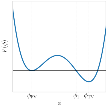
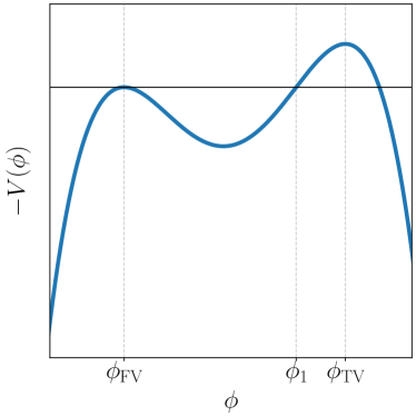
Figure 3: Left panel: asymmetric double-well potential with a local minimum in $\phi_{\rm FV}$ and a global one in $\phi_{\rm TV}$. Right panel: the same potential after the change of sign. $\phi_{1}$ labels the turning point.

Our goal is the computation of the probability per unit time $\gamma$ that the system, initially in the false vacuum configuration $\phi_{\rm FV}$, decays to the true vacuum configuration $\phi_{\rm TV}$. To this purpose, we consider our field theory as an ordinary quantum theory with an infinite number of degrees of freedom, labelled by points in three-dimensional space: $x_{i}(\tau)\rightarrow\phi_{{\textbf{x}}}(\tau)=\phi(\tau,{{\textbf{x}}})$. The formalism of Sect. 2.4 is readily generalized, to conclude that

$$\gamma=Ae^{-B},$$ (3.1)

where the overall factor $A$ is undetermined in the leading semi-classical approximation, while the exponent $B$ can be computed by a generalization of the argument presented in the previous section. In particular, we need bounce solutions $\phi_{b}(\tau,{\textbf{x}})$ to the Euclidean field equation

$$\left(\frac{\partial^{2}}{\partial\tau^{2}}+\bm{\nabla}^{2}\right)\phi_{b}(\tau,{\textbf{x}})=V^{\prime}(\phi_{b}),$$ (3.2)

with the boundary conditions

$$\lim_{\tau\to\pm\infty}\phi_{b}(\tau,{\textbf{x}})=\phi_{\rm FV}$$ (3.3)

$$\left.\frac{\partial\phi_{b}(\tau,{\textbf{x}})}{\partial\tau}\right|_{\tau=0}=0.$$ (3.4)

The exponent $B$ is then given by

$$B=S[\phi_{b}]-S[\phi_{\rm FV}],$$ (3.5)

where $S[\phi]$ is the Euclidean action of the theory,

$$S[\phi]=\int d^{4}x\,\left[\frac{1}{2}(\partial_{\mu}\phi)^{2}+V(\phi)\right].$$ (3.6)

By construction, the bounce solution $\phi_{b}$ approaches $\phi_{\rm FV}$, and hence $V(\phi_{b})\to V(\phi_{\rm FV})$, at infinite Euclidean time, see Eq. (3.3). By inspection of Eq. (3.5) we conclude that $\phi_{b}$ must approach $\phi_{\rm FV}$ also at space infinity, in order to keep the exponent $B$ finite:

$$\lim_{|\vec{x}|\to\infty}\phi_{b}(\tau,{\textbf{x}})=\phi_{\rm FV}.$$ (3.7)

The exponent $B$ can be written in a more compact form by using the virial theorem. Since the action, and hence $B$, is stationary in correspondence of solutions of the field equations, it will be stationary, in particular, upon variations of the following type:

$$\phi_{b}(x)\rightarrow\phi_{b}(ax).$$ (3.8)

After such transformations,

$$B\rightarrow B_{a} =\int d^{4}x\left[\frac{1}{2}\frac{\partial\phi_{b}(ax)}{\partial x_{\mu}}\frac{\partial\phi_{b}(ax)}{\partial x_{\mu}}+V(\phi_{b}(ax))-V(\phi_{\rm FV})\right]$$

$$=\frac{1}{a^{4}}\int d^{4}y\,\left[\frac{a^{2}}{2}\frac{\partial\phi_{b}(y)}{\partial y_{\mu}}\frac{\partial\phi_{b}(y)}{\partial y_{\mu}}+V(\phi_{b}(y))-V(\phi_{\rm FV})\right],$$ (3.9)

with the change of integration variable $y=ax$. The stationarity condition

$$\left.\frac{dB_{a}}{da}\right|_{a=1}=0$$ (3.10)

provides a relationship between the potential and the derivative terms in $B$, when computed at stationary points:

$$\int d^{4}x\,\frac{1}{2}\left(\partial_{\mu}\phi_{b}\right)^{2}=-2\int d^{4}x\,\left[V(\phi_{b})-V(\phi_{\rm FV})\right]$$ (3.11)

and therefore

$$B=-\int d^{4}x\,\left[V(\phi_{b})-V(\phi_{\rm FV})\right].$$ (3.12)

Before looking for an explicit bounce solution of the Euclidean field equation, it will be useful to illustrate its physical meaning. In ordinary quantum mechanics, the system initially occupies the false ground state; after an average time $T=1/\gamma$, the system simply makes a quantum jump and appears at the escape point beyond the barrier with zero kinetic energy (that is, the bounce configuration at time $\tau=0$). Afterwards, it evolves classically.

A similar picture holds in quantum field theory: at $\tau=0$ the field makes a quantum jump from the state in which it is uniformly equal to its false vacuum configuration, to the one described by the bounce solution, then it evolves classically. Therefore, the tunnelling process does not take place between two spatially uniform configurations, but rather from a spatially uniform one (the false vacuum) to a space-dependent one (the bounce), which, as we will see, has the shape of a bubble of true vacuum $\phi_{b}=\phi_{\rm TV}$ of finite radius, in a false vacuum $\phi_{b}=\phi_{\rm FV}$ background. Indeed, as we will show in more detail in Sect. 3.4, the tunnelling between two spatially homogeneous configurations would require penetration through an infinitely high potential energy barrier; the amplitude for such a process is zero. Instead we have a non-zero amplitude for the tunnelling between a spatially homogeneous configuration and one with a region of approximate true vacuum surrounded by a false vacuum background. This configuration then evolves classically, and eventually converts the false vacuum in the true vacuum everywhere in space. Since the bubble of true vacuum can appear anywhere, we expect the decay rate to be proportional to the volume of three-dimensional space $\mathcal{V}_{3}$.

The result, as described in Ref. [1], is closely similar to the boiling processes in a superheated fluid: the false vacuum corresponds to the superheated fluid state, while the true vacuum to the vapor state. Due to thermodynamical fluctuations, bubbles of vapor state appear at different points: when a bubble is large enough that the vapor pressure inside the bubble exceeds the external pressure plus the contribution of the surface tension, the bubble grows until it converts all the fluid into vapor, otherwise it shrinks back. By substituting thermodynamical fluctuations with quantum ones, this picture describes the decay of the false vacuum: once a bubble of true vacuum appears, large enough that its growth is energetically favourable, then it expands throughout the Universe, thereby achieving the transition to the true vacuum.

Let us go back to the problem of searching for a bounce solution of Eq. (3.2). It was shown in Ref. [14] that, if the field equation has bounce solutions, there always exists one bounce which is $\,{\rm O}(4)$ invariant, i.e. a function of

$$r=\sqrt{\tau^{2}+\left|{\textbf{x}}\right|^{2}}$$ (3.13)

alone, whose Euclidean action is smaller than that of any $\,{\rm O}(4)$ non-invariant bounce. We may therefore restrict our search to bounce solutions with $\,{\rm O}(4)$ invariance, $\phi_{b}(r)$. This simplifies considerably our task. Indeed, the field equation (3.2) becomes an ordinary differential equation:

$$\frac{d^{2}\phi_{b}}{dr^{2}}+\frac{3}{r}\frac{d\phi_{b}}{dr}=V^{\prime}(\phi_{b}),$$ (3.14)

while the two boundary conditions Eq. (3.3) and Eq. (3.7) combine into a single one:

$$\lim_{r\to\infty}\phi_{b}(r)=\phi_{\rm FV}.$$ (3.15)

Requiring that the solution is regular at ${\textbf{x}}=0$ we get the further boundary condition

$$\left.\frac{d\phi_{b}(r)}{dr}\right|_{r=0}=0.$$ (3.16)

3.2 Existence of a bounce solution

We now prove that a bounce solution with the correct boundary conditions actually exists in the case of an asymmetric double-well scalar potential $V(\phi)$ with a local minimum in $\phi=\phi_{\rm FV}$ and a global minimum in $\phi=\phi_{\rm TV}$. The proof was originally presented in Ref. [1]; here we reproduce the same argument almost word by word.

It is useful to view the field $\phi(r)$ as the position of a classical particle of unit mass in one dimension, as a function of the time $r$. Then the field equation, Eq. (3.14), can be regarded as the classical equation of motion of such a particle in a potential $-V$, which is further subject to a damping force with a time-dependent coefficient which decreases as $1/r$. The potential $-V$ is shown in the right panel of Fig. 3. We are looking for a solution $\phi_{b}(r)$ that starts at rest at $r=0$ from some initial value $\phi_{b}(0)$ and reaches $\phi_{b}=\phi_{\rm FV}$ with zero velocity at $r\to\infty$. We will demonstrate that such a solution exists by showing that if the initial position is too close to the left of $\phi_{\rm TV}$ then the particle passes through $\phi_{\rm FV}$ with non-zero velocity (the particle overshoots); if instead the initial position is too far to the left of from $\phi_{\rm TV}$, the particle does not reach $\phi_{\rm FV}$ (the particle undershoots). As a consequence, there must be an intermediate initial position such that the particle comes at rest exactly at $\phi_{\rm FV}$.

It is easy to demonstrate the undershoot: if the initial condition $\phi(0)$ is smaller than $\phi_{1}$, then the particle’s energy is smaller than the potential energy at $\phi=\phi_{\rm FV}$, which therefore cannot be reached. The presence of the viscous term just makes things worse by further lowering the energy; indeed, the energy $E$ is not conserved because of the viscous force, and

$$\frac{dE}{dr}=\frac{d}{dr}\left[\frac{1}{2}\left(\frac{d\phi}{dr}\right)^{2}-V(\phi)\right]=-\frac{3}{r}\left(\frac{d\phi}{dr}\right)^{2}<0$$ (3.17)

by the field equation.

The overshoot would also be obvious if we could neglect the damping force: the energy of a particle starting at rest with $\phi_{1}<\phi(0)<\phi_{\rm TV}$ would be larger than the potential energy at $\phi_{\rm FV}$, and would therefore reach $\phi_{\rm FV}$ with non-zero kinetic energy. The effect of the viscous term can be taken into account as follows. Let us take $\phi(0)$ to be close to $\phi_{\rm TV}$. For $\phi$ close to $\phi_{\rm TV}$ we may expand the potential in powers of $\phi-\phi_{\rm TV}$ up to second order:

$$V(\phi)=V(\phi_{\rm TV})+\frac{1}{2}\mu^{2}(\phi-\phi_{\rm TV})^{2}+O((\phi-\phi_{\rm TV})^{3}),$$ (3.18)

where $\mu^{2}=V^{\prime\prime}(\phi_{\rm TV})>0$. In this limit, Eq. (3.14) takes the form

$$\left(\frac{d^{2}}{dr^{2}}+\frac{3}{r}\frac{d}{dr}-\mu^{2}\right)\left[\phi(r)-\phi_{\rm TV}\right]=0.$$ (3.19)

It is easy to check that the solution of this equation is

$$\phi(r)-\phi_{\rm TV}=2\left[\phi(0)-\phi_{\rm TV}\right]\frac{I_{1}(\mu r)}{\mu r}$$ (3.20)

and $I_{1}(x)=-iJ_{1}(ix)$, where $J_{1}(x)$ is the Bessel function of order 1, solution of the differential equation

$$J_{1}^{\prime\prime}(x)+\frac{J_{1}^{\prime}(x)}{x}+\left(1-\frac{1}{x^{2}}\right)J_{1}(x)=0.$$ (3.21)

We see that, provided $\phi(0)$ is sufficiently close to $\phi_{\rm TV}$, the particle will spend an arbitrarily large amount of time in the vicinity of $\phi_{\rm TV}$. But after an arbitrarily large time $r$ the viscous term, which decreases as $r^{-1}$, becomes negligible, and in the absence of a damping force the particle overshoots. The announced result is therefore proved.

As an example, we have employed the overshoot-undershoot technique to find the bounce solution in the case of the scalar potential

$$V(\phi)=g\left[\frac{1}{4}\phi^{4}-\frac{1}{3}\phi^{3}(M+\phi_{\rm TV})+\frac{1}{2}\phi^{2}M\phi_{\rm TV}\right]$$ (3.22)

$$g>0;\qquad M=0.3\,\phi_{\rm TV},$$ (3.23)

which has a local minimum for $\phi=0$ and an absolute minimum for $\phi=\phi_{\rm TV}$. In fig. 4 we plot $h(x)=\frac{\phi(r)}{\phi_{\rm TV}}$ as a function of $x=\sqrt{g}r\phi_{\rm TV}$ for three different choices of $\phi(0)$. The first case is an undershoot: $\phi(0)$ is too much smaller than $\phi_{\rm TV}$, the particle gets close the false vacuum but then turns back and oscillates around $\phi=M$. Overshoot is shown in the second panel: the particle has too much energy to come at rest at $\phi=0$; it reaches the false vacuum with positive velocity, and goes on to negative values of the coordinate. In the third panel, $\phi(0)$ has the right value to reach the false-vacuum value $\phi=0$ at large $r$ with zero velocity.

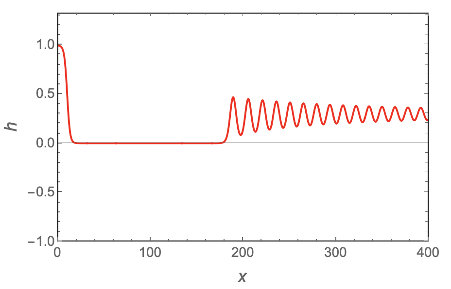
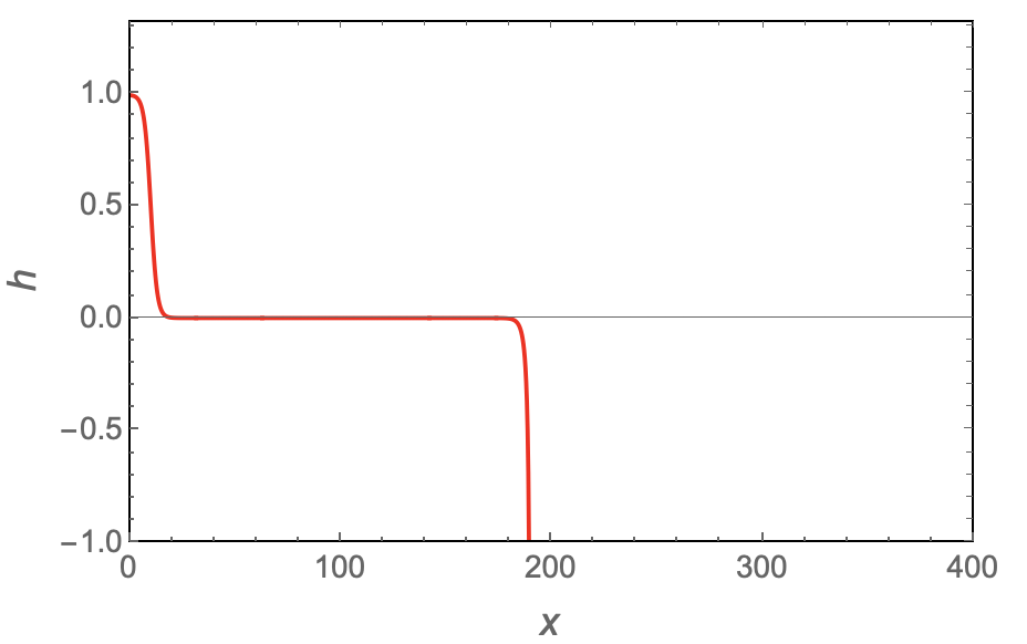
Figure 4: An example of the overshoot-undershoot mechanism.

The case when the two minima are nearly degenerate (in the above example, the case when $M$ is close to $\phi_{\rm TV}/2$) is especially interesting. This case corresponds to the so-called thin-wall approximation: the bounce is essentially a constant, equal to the true vacuum field value, for $r$ smaller than some value $R$, which is a function of the parameters in the theory. Then, within a small region around $r=R$ the bounce drops rapidly to the false vacuum field value. To an excellent approximation, the bounce is therefore a four-dimensional sphere of radius $R$ where the field takes the true-vacuum value, while $\phi=\phi_{\rm FV}$ in the rest of Euclidean space-time. In the thin-wall approximation, the calculation of the tunnelling rate can be carried on analytically; the leading semi-classical tunnelling rate (that is, the exponent $B$) was computed in the original Coleman’s paper [1], while a closed-form calculation at one loop in this limit has been presented recently [15].

To summarize, the decay probability per unit time of a metastable state in the leading semi-classical approximation is given by

$$\gamma=Ae^{-B}$$ (3.24)

where

$$B =S[\phi_{b}]-S[\phi_{\rm FV}]$$

$$=\int d^{4}x\,\left[\frac{1}{2}\partial_{\mu}\phi_{b}\partial_{\mu}\phi_{b}+V(\phi_{b})-V(\phi_{\rm FV})\right]$$

$$=-\int d^{4}x\,[V(\phi_{b})-V(\phi_{\rm FV})]$$ (3.25)

where $\phi_{b}(r)$ is the $O(4)$-invariant bounce. The overall factor $A$ is undetermined in the leading semi-classical limit; we expect it to be proportional to the three-dimensional volume ${\mathcal{V}}_{3}$ as a consequence of integration over the position of the true-vacuum bubble. This expectation will be confirmed by the inclusion of the first quantum corrections.

3.3 Time evolution of the true-vacuum bubble

The decay of the false vacuum takes place as illustrated in Sect. 3.1: at some Euclidean time, say $\tau=0$, and at some point x of three-dimensional space, an $O(4)$-symmetric bubble of true vacuum is formed in the false-vacuum background by quantum fluctuations:

$$\phi_{b}(|{\textbf{x}}|)=\phi_{\rm TV};\qquad\left.\frac{\partial}{\partial\tau}\phi_{b}\left(\sqrt{|{\textbf{x}}|^{2}+\tau^{2}}\right)\right|_{\tau=0}=0;\qquad\lim_{\tau\to\infty}\phi_{b}\left(\sqrt{|{\textbf{x}}|^{2}+\tau^{2}}\right)=\phi_{\rm FV}.$$ (3.26)

Then, the bubble evolves in real (i.e. Minkowski space) time according to the classical equations of motion. The qualitative behavior of the bubble is easy to obtain by analytical continuation of the bounce to Minkowski space:

$$\phi_{b}(\sqrt{|{\textbf{x}}|^{2}+\tau^{2}})\ \to\ \phi_{b}(\sqrt{|{\textbf{x}}|^{2}-t^{2}}).$$ (3.27)

To visualize the time evolution of the bubble, we may study the time dependence of the three-dimensional surface in space-time separating the true vacuum region from the false vacuum background, which in the thin-wall limit is the hyperbole

$$|{\textbf{x}}|^{2}-t^{2}=R^{2}.$$ (3.28)

We find that the bubble expands in three-dimensional space with velocity

$$v=\frac{1}{\sqrt{1+\frac{R^{2}}{t^{2}}}},$$ (3.29)

which approches the velocity of light as $t\to\infty$ quite rapidly: for example, we shall see that $R\sim 10^{-16}\,{\rm GeV}^{-1}\sim 10^{-40}\,{\rm s}$ in the case of the standard model.

3.4 Potential barriers in quantum field theory

This section is devoted to a discussion of a feature of tunnelling phenomena in quantum field theory which may appear as counter-intuitive, and deserves some comments. In some cases, tunnelling from a metastable ground state to a lower minimum configuration takes place even if the scalar potential of the theory, considered as an ordinary function of the scalar fields, has no barrier in the usual sense.

This apparent paradox can be explained by observing that the tunnelling process in quantum field theory does not take place between two spatially homogeneous field configurations, but rather through the formation of a bubble of true vacuum in a false-vacuum background. Such field configuration (the bounce) is therefore not spatially homogenous, and the gradient term in the potential energy gives a non-zero contribution to the full potential energy.

In order to identify a quantity with the same properties as a potential barrier in ordinary quantum mechanics, it will be useful to cast the exponent in the semi-classical decay rate

$$B=S[\phi_{b}]=\int d^{4}x\,\left[\frac{1}{2}\left(\partial_{\mu}\phi_{b}\right)^{2}+V(\phi_{b})\right]$$ (3.30)

(we are now taking $V(\phi_{\rm FV})=0$) in a form similar to the WKB formula for the exponential factor in quantum mechanics, Eq. (2.165),

$$B_{\rm QM}=2\int_{0}^{s_{f}}ds\,\sqrt{2U({\textbf{x}}(s))}$$ (3.31)

where $U({\textbf{x}})$ is the potential energy and the integral is taken over a a suitable path ${\textbf{x}}={\textbf{x}}(s)$ in configuration space, which connects the local minimum to a point beyond the potential barrier. This section is devoted to the identification of such a quantity, following an argument originally presented by K.M. Lee and E.J. Weinberg in Ref. [16].

Our starting point is the Lagrangian density of a scalar theory in Eucidean time

$${\mathcal{L}}=-\frac{1}{2}\left(\frac{\partial\phi}{\partial\tau}\right)^{2}-\frac{1}{2}\left(\bm{\nabla}\phi\right)^{2}-V(\phi)$$ (3.32)

and the corresponding Hamiltonian density

$${\mathcal{H}}=-\frac{1}{2}\left(\frac{\partial\phi}{\partial\tau}\right)^{2}+\frac{1}{2}\left(\bm{\nabla}\phi\right)^{2}+V(\phi).$$ (3.33)

We assume that the total energy

$$E[\phi]=\int d^{3}x\,{\mathcal{H}}$$ (3.34)

has a local minimum (the false vacuum) for a constant and uniform configuration of the field $\phi=\phi_{\rm FV}$. We define the potential energy $U[\phi]$ as the term in the total energy that does not contain time derivatives of the field:

$$U[\phi]=\int d^{3}x\,\left[\frac{1}{2}\left(\bm{\nabla}\phi\right)^{2}+V(\phi)\right],$$ (3.35)

which is a functional of the field $\phi$ and an ordinary function of the Euclidean time $\tau$. Then the Euclidean action can be written as

$$S[\phi]=-\int d^{3}x\,d\tau\,\mathcal{L}=\int d^{3}x\,\left\{\int_{-\infty}^{\infty}d\tau\,\frac{1}{2}\left(\frac{\partial\phi}{\partial\tau}\right)^{2}+\int_{-\infty}^{\infty}d\tau\,U[\phi]\right\}.$$ (3.36)

For $\phi=\phi_{b}$, this formula can be simplified by energy conservation: the total energy of the system in the false vacuum configuration must be the same as the energy in the bounce configuration:

$$E[\phi_{\rm FV}]=E[\phi_{b}],$$ (3.37)

which is zero by our choice of the additive constant in the scalar potential. Hence

$$E[\phi_{b}]=-\frac{1}{2}\int d^{3}x\,\left(\frac{\partial\phi_{b}}{\partial\tau}\right)^{2}+U[\phi_{b}]=0$$ (3.38)

which gives

$$U[\phi_{b}]=\frac{1}{2}\int d^{3}x\,\left(\frac{\partial\phi_{b}}{\partial\tau}\right)^{2}.$$ (3.39)

Thus,

$$S[\phi_{b}]=\int_{-\infty}^{\infty}d\tau\,2U[\phi_{b}].$$ (3.40)

To complete the analogy with Eq. (3.31), we perform a change of integration variable in Eq. (3.40) from $\tau$ to $s$, defined by

$$ds^{2}=\int d^{3}x\,\left[d\phi_{b}(x)\right]^{2},$$ (3.41)

in analogy with the infinitesimal path length defined in the case of quantum mechanics with many degrees of freedom,

$$\sum_{i}\frac{dx_{i}}{ds}\frac{dx_{i}}{ds}=1;\qquad ds^{2}=\sum_{i}dx_{i}^{2}.$$ (3.42)

We have therefore

$$\left(\frac{ds}{d\tau}\right)^{2}=\int d^{3}x\,\left(\frac{\partial\phi_{b}}{\partial\tau}\right)^{2}=2U[\phi_{b}],$$ (3.43)

where in the second step we have used Eq. (3.39). This allows us to write Eq. (3.40) as

$$S[\phi_{b}]=\int_{-\infty}^{\infty}d\tau\,2U[\phi_{b}]=2\int_{0}^{\infty}d\tau\,2U[\phi_{b}]=2\int_{\gamma}ds\,\frac{d\tau}{ds}2U[\phi_{b}]=2\int_{\gamma}ds\,\sqrt{2U[\phi_{b}]},$$ (3.44)

where $\gamma$ is the path in configuration space. We have therefore achieved our goal: we have written the Euclidean action as a line integral over a path in configuration space. Correspondingly, $U[\phi_{b}]$ can be considered as the quantum field theory generalization of the potential barrier of ordinary quantum mechanics, as one can check by comparison with Eq. (3.31). It is important to emphasize that the integral is independent of the parametrization chosen for the path, which is the one which minimizes the Euclidean action.

The potential energy $U[\phi_{b}]$ is the sum of a potential term $U_{V}[\phi_{b}]$ and a gradient term $U_{\nabla}[\phi_{b}]$:

$$U[\phi_{b}]=U_{\nabla}[\phi_{b}]+U_{V}[\phi_{b}]$$ (3.45)

$$U_{\nabla}[\phi_{b}]=\int d^{3}x\,\frac{1}{2}\left(\bm{\nabla}\phi_{b}\right)^{2}$$ (3.46)

$$U_{V}[\phi_{b}]=\int d^{3}x\,V(\phi_{b}).$$ (3.47)

The identification of $U[\phi_{b}]$ as the barrier in quantum field theory allows us to draw some interesting consequences.

• It is now clear why tunnelling in quantum field theory requires bounce solutions and cannot directly take place as a transition between spatially homogeneous configurations: the barrier associated with such a tunnelling process would be infinitely high. Specifically, in such cases we would find $U_{\nabla}[\phi_{b}]=0$ and $U_{V}[\phi_{b}]$ proportional to the space volume ${\mathcal{V}}_{3}$.

• The gradient and the potential terms may have opposite signs: even if the scalar potential has no barrier separating different minima, a potential energy barrier may appear because of the gradient term. An important examples of this class is the standard model, as we shall see in Sect. 5.6.

• The barrier penetration integral $B=S[\phi_{b}]$ is calculated as an integral over the three-dimensional space. In particular, the potential term is obtained by integrating the scalar potential, computed at the bounce configuration. Hence, the value of $S[\phi_{b}]$ is affected by all energy scales between $0$ and $\phi_{b}(0)$. We will come back to this issue in Sect. 5.6, when discussing the impact of non-standard physics on the metastability of the electroweak ground state.

3.5 Quantum corrections

The first quantum corrections to the leading semi-classical approximation of the decay rate of an unstable ground state are computed [2] by a generalization to quantum field theory of the analogous calculation, presented in Sect. 2.3, of the tunnelling rate in the case of an ordinary quantum theory with many degrees of freedom. This generalization is rather straightforward, except for a few differences, which must be taken into proper account.

3.5.1 Zero modes

In the case of ordinary quantum mechanics, a factor of $\sqrt{\frac{S[x_{b}]-S[x_{0}]}{2\pi\hbar m}}$ appears as a consequence of the presence of a zero mode in the spectrum of the second derivative of the action due time translation invariance. Here we have four such factors (with $m=1$), corresponding to one zero mode for translations in each space-time direction. Correspondingly, the integration over all possible bounce centers, which yields a factor of $T$ in the case of ordinary quantum mechanics in one space dimension, is now replaced by an integration over all possible bounce centers in space-time, yielding a factor of $T{\mathcal{V}}_{3}$, where ${\mathcal{V}}_{3}$ is the three-dimensional volume.

This is a good place for a more general discussion of zero modes of the second derivative of the action, which will turn out to play an important role in the application of the formalism to the standard model. In general, zero modes of $S^{\prime\prime}[\phi_{b}]$ appear whenever the theory has an invariance property under a class of transformations of the field which we define in infinitesimal form as

$$\phi(x)\to\phi^{\prime}(x)=\phi(x)+\epsilon\Delta\phi(x).$$ (3.48)

In such case,

$$\Delta\phi_{b}(x)=\frac{\partial\phi^{\prime}_{b}(x)}{\partial\epsilon}$$ (3.49)

is a zero mode of $S^{\prime\prime}[\phi_{b}]$. Here is the proof. As a consequence of the invariance of the theory upon the transformations Eq. (3.48), $\phi^{\prime}_{b}(x)$ is also a bounce solution, and $S[\phi_{b}^{\prime}]=S[\phi_{b}]$. Therefore

$$S^{\prime\prime}[\phi_{b}]\Delta\phi_{b}=S^{\prime\prime}[\phi^{\prime}_{b}]\frac{\partial\phi^{\prime}_{b}}{\partial\epsilon}=(-\partial^{2}+V^{\prime\prime}(\phi^{\prime}_{b}))\frac{\partial\phi^{\prime}_{b}}{\partial\epsilon}=\frac{\partial}{\partial\epsilon}(-\partial^{2}+V^{\prime}(\phi^{\prime}_{b}))\phi^{\prime}_{b}=0$$ (3.50)

by the field equations. For example, under an infinitesimal translation

$$x_{\mu}\to x_{\mu}+\epsilon_{\mu}$$ (3.51)

the bounce transforms as

$$\phi_{b}(x)\to\phi^{\prime}_{b}(x)=\phi_{b}(x+\epsilon)=\phi_{b}(x)+\epsilon_{\mu}\partial_{\mu}\phi_{b}(x).$$ (3.52)

If the theory is invariant under translations, then

$$\phi_{\mu}(x)=N\partial_{\mu}\phi_{b}(x)$$ (3.53)

are four zero modes of $S^{\prime\prime}[\phi_{b}]$. The normalization factor $N$ is finite: Eqs. (3.5, 3.11, 3.12) give

$$\int d^{4}x\,(\partial_{\mu}\phi_{b})^{2}=4\left(S[\phi_{b}]-S[\phi_{\rm FV}]\right),$$ (3.54)

so

$$N=\frac{1}{\sqrt{S[\phi_{b}]-S[\phi_{\rm FV}]}}.$$ (3.55)

From our experience in quantum mechanics, we know how to deal with these zero modes in the computation of the path integral: the calculation of the path integral is performed by integrating over all possible values of the coefficients $c_{i}$ of the expansion of the scalar field in the basis of orthonormal eigenfunctions of $S^{\prime\prime}[\phi]$, which includes normalized zero-modes:

$$\phi(x)=\phi_{b}(x)+\sum_{i}c_{i}\phi_{i}(x)=\phi_{b}(x)+c_{\mu}N\partial_{\mu}\phi_{b}(x)+\ldots.$$ (3.56)

As a consequence, integrating over $c_{\mu}$ is equivalent to integrating over all possible locations of the bounce center:

$$\frac{dc_{\mu}}{\sqrt{2\pi}}=\frac{1}{\sqrt{2\pi}}\frac{d\epsilon_{\mu}}{N}=\sqrt{\frac{S[\phi_{b}]-S[\phi_{\rm FV}]}{2\pi}}d\epsilon_{\mu}.$$ (3.57)

These integrations contribute to the path integral a factor of

$$\left[\sqrt{\frac{S[\phi_{b}]-S[\phi_{\rm FV}]}{2\pi}}\right]^{4}{\mathcal{V}}_{3}T$$ (3.58)

where ${\mathcal{V}}_{3}T$ is the space-time volume; note however that the integration in the directions of zero-modes can be converted into an integration over a collective coordinate (the bounce center in this case) only provided that the zero-modes are normalizable.

One might wonder whether analogous zero modes arise from Lorentz transformations, which in Eulidean space-time correspond to 4-dimensional rotations. The six functions

$$\phi_{\mu\nu}(x)=\left(x_{\mu}\partial_{\nu}-x_{\nu}\partial_{\mu}\right)\phi_{b}(x)$$ (3.59)

are in fact eigenfunction of $S^{\prime\prime}[\phi_{b}]$ with zero eigenvalues, as one can check directly. However, they vanish because of the above-mentioned $\,{\rm O}(4)$ invariance of the bounce.

To conclude this section we mention two more possible origins of zero modes; both will be discussed in more detail in Sect. 5. The first one is the presence of an internal symmetry. The simplest example is a complex scalar theory, invariant under $U(1)$ transformations

$$\phi(x)\to\phi^{\prime}(x)=\phi(x)+i\epsilon\phi(x).$$ (3.60)

In this case and $\Delta\phi_{b}(x)=i\phi_{b}(x)$ is a zero mode. The corresponding contribution to the path integral is obtained integrating over all possible $U(1)$ transformations:

$$\frac{dc}{\sqrt{2\pi}}=\frac{1}{\sqrt{2\pi}}\frac{d\epsilon}{N}=\frac{d\epsilon}{\sqrt{2\pi}}\left[\int d^{4}x\,|\phi_{b}(x)|^{2}\right]^{-\frac{1}{2}}.$$ (3.61)

The integration contributes to the path integral a factor of

$$\frac{{\mathcal{V}}}{\sqrt{2\pi}}\left[\int d^{4}x\,|\phi_{b}(x)|^{2}\right]^{-\frac{1}{2}}$$ (3.62)

where ${\mathcal{V}}=2\pi$ is the volume of the symmetry group. In this case, the bounce itself must be normalizable. A full discussion of the impact on the calculation of the path integral of internal symmetry zero modes is presented in Ref. [17]; quite obviously, they play a role in the case of the standard model.

As a final example, let us assume that the theory is invariant upon scale transformations, defined by

$$\phi(x)\to\phi^{\prime}(x)=e^{\epsilon d}\phi(e^{\epsilon}x),$$ (3.63)

where $d$ is the mass dimension of the field ($d=1$ for boson fields in four space-time dimensions). In infinitesimal form

$$\phi(x)\to\phi^{\prime}(x)=\phi(x)+\epsilon(1+x_{\mu}\partial_{\mu})\phi(x).$$ (3.64)

Then, by the argument given above,

$$\phi_{s}(x)=(1+x_{\mu}\partial_{\mu})\phi_{b}(x)$$ (3.65)

is a zero mode of $S^{\prime\prime}[\phi_{b}]$. This example is especially interesting, because the only scale-invariant theories of one scalar fields in four dimensions are specified by the scalar potential

$$V(\phi)=\frac{1}{4}\lambda\phi^{4},$$ (3.66)

with $\lambda$ a constant, which is an excellent approximation of the standard model scalar potential at large field values. Furthermore, the field equation for an $\,{\rm O}(4)$-invariant bounce,

$$\frac{d^{2}\phi_{b}(r)}{dr^{2}}+\frac{3}{r}\frac{d\phi_{b}(r)}{dr}=\lambda\phi_{b}^{3}(r)$$ (3.67)

has an analytical solution for $\lambda<0$:

$$\phi_{b}(r)=\frac{\phi_{b}(0)}{1+\frac{|\lambda|}{8}\phi_{b}^{2}(0)r^{2}},$$ (3.68)

usually referred to as the Fubini-Lipatov bounce, originally presented in Refs. [18, 19] (alternative derivations of Eq. (3.68) can be found in Ref. [16] and in Ref. [20]; the latter is reviewed in App. A.5.)

Unfortunately, the zero mode of scale transformations

$$\phi_{s}(r)=(1+x_{\mu}\partial_{\mu})\phi_{b}(x)=\phi_{b}(0)\frac{1-\frac{|\lambda|}{8}\phi_{b}^{2}(0)r^{2}}{\left(1+\frac{|\lambda|}{8}\phi_{b}^{2}(0)r^{2}\right)^{2}}$$ (3.69)

is not normalizable: $\phi^{2}_{s}(r)\sim r^{-4}$ for $r\to\infty$. It follows that the corresponding contribution to the path integral cannot be replaced by an integration over a collective coordinate, as in the case of translation zero modes.

3.5.2 Renormalization

A second important difference between quantum field theory and ordinary quantum mechanics is the appearance of ultraviolet divergences in the computation of the action beyond the semi-classical approximation. Ultraviolet divergences require the usual renormalization procedure; specifically, the classical action must be expressed in terms of renormalized fields and parameters, and supplemented by appropriate counterterms:

$$S[\phi]\to S[\phi]+\hbar S_{\rm ct}[\phi]$$ (3.70)

where $S_{\rm ct}[\phi]$ is the action induced by one-loop counterterms, and we have (temporarily) restored the dependence on $\hbar$ for later convenience. In general, the presence of the counterterms will modify the bounce solution:

$$\phi_{b}\to\phi_{b}+\hbar\phi_{\rm ct}$$ (3.71)

where $\phi_{b}$ is a bounce solution for $S[\phi]$:

$$\left.\frac{\delta S[\phi]}{\delta\phi}\right|_{\phi=\phi_{b}}=0.$$ (3.72)

However, to one-loop order, the explicit expression of the correction $\phi_{\rm ct}$ is not needed. Indeed,

$$S[\phi_{b}+\hbar\phi_{\rm ct}]+\hbar S_{\rm ct}[\phi_{b}+\hbar\phi_{\rm ct}]$$

$$=S[\phi_{b}]+\hbar\int d^{4}x\,\phi_{\rm ct}\left.\frac{\delta S[\phi]}{\delta\phi}\right|_{\phi=\phi_{b}}+\hbar S_{\rm ct}[\phi_{b}]+O(\hbar^{2})$$

$$=S[\phi_{b}]+\hbar S_{\rm ct}[\phi_{b}]+O(\hbar^{2}).$$ (3.73)

Taking these differences into proper account, and setting back $\hbar=1$, we obtain the following result for the decay probability per unit time and per unit volume $\gamma/{\mathcal{V}}_{3}$ of a metastable state:

$$\frac{\gamma}{{\mathcal{V}}_{3}}=\frac{\left(S[\phi_{b}]-S[\phi_{\rm FV}]\right)^{2}}{(2\pi)^{2}}\sqrt{\frac{\mbox{Det}\,S^{\prime\prime}[\phi_{\rm FV}]}{|\mbox{Det}\,^{\prime}S^{\prime\prime}[\phi_{b}]|}}e^{-\left(S[\phi_{b}]-S[\phi_{\rm FV}]\right)}e^{-\left(S_{\rm ct}[\phi_{b}]-S_{\rm ct}[\phi_{\rm FV}]\right)},$$ (3.74)

Eq. (3.74) is dimensionally correct: since there are four zero modes, the pre-exponential factor has the dimension of the square root of $S^{\prime\prime}[\phi]$ (an inverse length) to the fourth power.

4 The effective potential

The appropriate tool to determine the ground state of a quantum field theory beyond tree level is the effective potential [21, 22], since it automatically encodes radiative corrections while retaining the advantage of the semi-classical approximation, namely the possibility of simultaneously surveying all the vacua of the theory by minimizing a function in analogy to the tree-level potential. Furthermore, we have seen in the previous sections that functional methods are extremely useful in the study of the lifetime of metastable states in quantum field theory.

In this section we briefly review the effective action formalism and apply it to the case of the standard model of electroweak interactions, in order to study the possible instability of the ground state at large field values.

4.1 Effective action and effective potential

Let us consider the theory of a single real scalar field $\Phi$ described by the Lagrangian density $\mathcal{L}(\Phi,\partial_{\mu}\Phi)$ with a linear coupling of $\Phi(x)$ to an external source $J(x)$:

$$\mathcal{L}\to\mathcal{L}+J(x)\Phi(x).$$ (4.1)

The vacuum-to-vacuum transition amplitude $Z[J]$ is usually written in terms of a functional $W[J]$ as

$$Z[J]=\braket{0}{0}_{J}\equiv e^{iW[J]}=\int\mathcal{D}\Phi\,e^{i\int d^{4}x\,\left[\mathcal{L}(\Phi,\partial_{\mu}\Phi)+J\Phi\right]},$$ (4.2)

where in the last step we have employed the standard path integral representation. Functional derivatives of $W[J]$ with respect to $iJ$ at $J=0$ give the connected Green’s functions of the theory; for this reason, $W[J]$ is called the connected generating functional. $W[J]$ admits a functional Taylor expansion

$$W[J]=\sum_{n}\frac{i^{n}}{n!}\int d^{4}x_{1}\ \dots\ d^{4}x_{n}G^{(n)}(x_{1},\dots,x_{n})J(x_{1})\dots J(x_{n}),$$ (4.3)

where $G^{(n)}$ denotes the $n$-point connected Green’s functions. These, in turn, are computed in perturbation theory as the sum of all connected Feynman diagrams with $n$ external lines.

Next, one then defines the classical field $\phi_{c}(x)$ as

$$\phi_{c}(x)\equiv\frac{\delta W[J]}{\delta J(x)}=\frac{\bra{0}\Phi(x)\ket{0}_{J}}{\braket{0}{0}_{J}},$$ (4.4)

where the last expression follows from the path integral representation in Eq. (4.2). Note that $\phi_{c}(x)$ is by definition a functional of $J$; we are implicitly assuming that this functional is single-valued. This is related to the convexity issue of the effective potential, to be discussed in Sect. 4.6. We now introduce the effective action $\Gamma[\phi_{c}]$, defined by the functional Legendre transformation

$$\Gamma[\phi_{c}]=W[J]-\int d^{4}x\ J(x)\phi_{c}(x).$$ (4.5)

The effective action can be expanded in powers of the classical fields, in a way similar to Eq. (4.3), yielding

$$\Gamma[\phi_{c}]=\sum_{n=0}^{\infty}\frac{1}{n!}\int dx_{1}\dots dx_{n}\Gamma^{(n)}(x_{1},\dots,x_{n})\phi_{c}(x_{1})\dots\phi_{c}(x_{n}).$$ (4.6)

The coefficients $\Gamma^{(n)}$ can be shown to correspond to the one-particle-irreducible (1PI) Green’s functions of the theory (see for example Ref. [11]).

The functional $\Gamma[\phi_{c}]$ is the appropriate tool to study spontaneous symmetry breaking. Indeed, the condition for spontaneous symmetry breaking is that $\phi_{c}$ is different from zero even when the source $J$ is equal to zero, as can be read off Eq. (4.4). On the other hand, one has

$$\frac{\delta\Gamma[\phi_{c}]}{\delta\phi_{c}(x)}=\int d^{4}y\ \frac{\delta W[J]}{\delta J(y)}\frac{\delta J(y)}{\delta\phi_{c}(x)}-J(x)-\int d^{4}y\ \frac{\delta J(y)}{\delta\phi_{c}(x)}\phi_{c}(y)=-J(x),$$ (4.7)

or in other words

$$\left.\frac{\delta\Gamma[\phi_{c}]}{\delta\phi_{c}(x)}\right|_{J=0}=0.$$ (4.8)

We conclude that spontaneous symmetry breaking takes place when the classical field that minimizes the effective action is different from zero.

The effective action can be computed in perturbation theory by the usual technique of Feynman diagram. In particular, it can be shown that in the tree-level approximation the effective action coincides with the classical action:

$$\Gamma[\phi_{c}]=\int d^{4}x\,\left[{\mathcal{L}}(\phi_{c},\partial_{\mu}\phi_{c})+J\phi_{c}\right]+\text{loop corrections}.$$ (4.9)

In some cases, however, an expansion in powers of external momenta is more useful. To define such an expansion, we consider the Fourier transforms of the functions $\Gamma^{(n)}(x_{1},\dots,x_{n})$:

$$\Gamma^{(n)}(x_{1},\dots,x_{n}) =\int\frac{d^{4}p_{1}}{(2\pi)^{4}}\ldots\frac{d^{4}p_{n}}{(2\pi)^{4}}e^{i(p_{1}x_{1}+\dots+p_{n}x_{n})}$$

$$\times(2\pi)^{4}\delta(p_{1}+\ldots+p_{n})\tilde{\Gamma}^{(n)}(p_{1},\ldots,p_{n}),$$ (4.10)

and expand $\tilde{\Gamma}^{(n)}$ in powers of momenta around $p_{i}=0$:

$$\tilde{\Gamma}^{(n)}(p_{1},\ldots,p_{n})=\tilde{\Gamma}^{(n)}(0)+\ldots.$$ (4.11)

The effective action becomes

$$\Gamma[\phi_{c}] =\sum_{n=0}^{\infty}\frac{1}{n!}\int dx_{1}\dots dx_{n}\,\phi_{c}(x_{1})\dots\phi_{c}(x_{n})$$

$$\times\int\frac{d^{4}p_{1}}{(2\pi)^{4}}\ldots\frac{d^{4}p_{n}}{(2\pi)^{4}}e^{i(p_{1}x_{1}+\dots+p_{n}x_{n})}\int d^{4}x\,e^{-ix(p_{1}+\ldots+p_{n})}\left[\tilde{\Gamma}^{(n)}(0)+\ldots\right]$$

$$=\int d^{4}x\,\sum_{n=0}^{\infty}\frac{1}{n!}\tilde{\Gamma}^{(n)}(0)\phi^{n}_{c}(x)+\ldots.$$ (4.12)

The first term in this expansion is usually written as

$$-\int d^{4}x\,V_{\rm eff}(\phi_{c}),$$ (4.13)

where

$$V_{\rm eff}(\phi_{c})=-\sum_{n=0}^{\infty}\frac{1}{n!}\tilde{\Gamma}^{(n)}(0)\phi^{n}_{c}$$ (4.14)

is an ordinary function of $\phi_{c}$, usually called the effective potential of the theory, since it does not contain derivatives of the classical field. The following terms, originating from higher powers of momenta in the expansion of $\tilde{\Gamma}^{(n)}$, contain instead two or more derivatives of $\phi_{c}$.

If we require translational invariance of the vacuum state, then $\partial_{\mu}\phi_{c}=0$ for $J=0$, and the minimum condition Eq. (4.8) reduces to

$$\frac{dV_{\rm eff}(\phi_{c})}{d\phi_{c}}=0.$$ (4.15)

The advantage of Eq. (4.15) is that the ground state of the theory can be determined, including quantum corrections, via the minimization of a single ordinary function, the effective potential, in analogy with the tree-level case.

4.2 The background field method

The discussion of the previous section shows that efficient techniques for the computation of the effective potential are needed. A compact way to compute the loop-expanded effective potential is given by the background field method [23], which we review here for the one-loop case. Let us consider the Lagrangian density for a real scalar field $\Phi$:

$$\mathcal{L}(\Phi,\partial_{\mu}\Phi)=\frac{1}{2}\partial_{\mu}\Phi\partial^{\mu}\Phi-V(\Phi),$$ (4.16)

with $V(\Phi)$ denoting the tree-level scalar potential. We perform the following change of variable in the functional integral Eq. (4.2):

$$\Phi(x)=\phi_{c}(x)+\phi(x)\,$$ (4.17)

where $\phi_{c}(x)$ is a background field which we identify with the classical field of the previous section, while $\phi(x)$ is a dynamical (quantum) field. Organized in powers of $\phi$ (up to quadratic terms), the exponent of the r.h.s. of Eq. (4.2) takes the form

$$\int d^{4}x\,\left[\mathcal{L}(\phi_{c}+\phi)+J(\phi_{c}+\phi)\right]$$

$$\qquad=\int d^{4}x\,\left[\mathcal{L}(\phi_{c})+J\phi_{c}\right]+\int d^{4}x\,\phi(x)\left[\left.\frac{\delta\mathcal{L}}{\delta\Phi}\right|_{\Phi=\phi_{c}}+J\right]$$

$$\qquad+\frac{1}{2}\int d^{4}x\,d^{4}y\,\phi(x)i\mathscr{D}^{-1}(\phi_{c},x-y)\phi(y)+\mathcal{O}(\phi^{3}),$$ (4.18)

where

$$i\mathscr{D}^{-1}(\phi_{c},x-y) =\left.\frac{\delta}{\delta\Phi(x)}\frac{\delta}{\delta\Phi(y)}\int d^{4}z\,\left[\mathcal{L}(\Phi)+J(z)\Phi(z)\right]\right|_{\Phi=\phi_{c}}$$

$$=\left[-\partial^{2}-V^{\prime\prime}(\phi_{c}(x))\right]\delta^{(4)}(x-y)$$ (4.19)

is the inverse propagator in configuration space evaluated at $\Phi=\phi_{c}$. We can now explicitly perform the path integral in the gaussian approximation:

$$e^{iW[J]} \simeq e^{i\int d^{4}x\,\left[\mathcal{L}(\phi_{c})+J\phi_{c}\right]}\int\mathcal{D}\phi\,\exp{\left(\frac{i}{2}\int d^{4}x\,d^{4}y\,\phi(x)i\mathscr{D}^{-1}(\phi_{c},x-y)\phi(y)\right)}$$

$$=\mathcal{N}e^{i\int d^{4}x\,\left[\mathcal{L}(\phi_{c})+J\phi_{c}\right]}\left[\mbox{det}\,i\mathscr{D}^{-1}(\phi_{c},x-y)\right]^{-\frac{1}{2}},$$ (4.20)

up to an irrelevant normalization constant $\mathcal{N}$. The result Eq. (4.2) follows from the invariance of the path integral measure, $\mathcal{D}\Phi=\mathcal{D}\phi$, and the classical field equation $\left.\frac{\delta\mathcal{L}}{\delta\Phi}\right|_{\phi_{c}}+J=0$. The latter approximation is sufficient as long as we are interested in the one-loop effective action. After replacing Eq. (4.2) in the definition of the effective action, Eq. (4.5), we obtain

$$\Gamma[\phi_{c}]=S[\phi_{c}]+\frac{i}{2}\log\mbox{Det}\,i\mathscr{D}^{-1}(\phi_{c},x-y),$$ (4.21)

where

$$S[\phi_{c}]=\int d^{4}x\,\mathcal{L}(\phi_{c},\partial_{\mu}\phi_{c})$$ (4.22)

is the classical action. The calculation of one-loop corrections to the effective action involves the usual renormalization procedure: although not explicitly shown in Eq. (4.21), it is understood that the final result involves the choice of a regularization procedure and of a renormalization scheme, and the introduction of suitable counterterms. Typically, this results in the dependence of the renormalized parameters on an arbitrary energy scale, to compensate the explicit dependence of the correction term on the same scale.

The effective potential is now immediately obtained by evaluating Eq. (4.21) for a space-time-independent classical field configuration $\phi_{c}$ (see Eq. (4.1)). We get

$$-\mathcal{V}_{4}\ V_{\rm eff}(\phi_{c})=-\mathcal{V}_{4}\ V_{0}(\phi_{c})+\frac{i}{2}\log\mbox{Det}\,i\mathscr{D}^{-1}(\phi_{c},x-y),$$ (4.23)

where $\mathcal{V}_{4}\equiv\int d^{4}x$ denotes the space-time volume, originating from the fact that $\phi_{c}$ is space-time independent. The homogeneity of $\phi_{c}$ also allows for a simple evaluation of the functional determinant, through the identity

$$\log\mbox{Det}\,i\mathscr{D}^{-1}(\phi_{c},x-y)=\mbox{tr}\,\log i\mathscr{D}^{-1}(\phi_{c},x-y).$$ (4.24)

The functional trace, denoted by tr , is taken by setting $x=y$ and integrating over the space-time. This gives

$$\log\mbox{Det}\,i\mathscr{D}^{-1}(\phi_{c},x-y)=\mathcal{V}_{4}\log i\mathscr{D}^{-1}(\phi_{c},0)=\mathcal{V}_{4}\int\frac{d^{4}k}{(2\pi)^{4}}\log i\tilde{\mathscr{D}}^{-1}(\phi_{c},k),$$ (4.25)

where $\tilde{\mathscr{D}}^{-1}(\phi_{c},k)$ denotes the four-dimensional Fourier transform of $\mathscr{D}^{-1}(\phi_{c},x-y)$.

An explicit example is provided by a renormalizable scalar theory, with

$$V_{0}(\Phi)=\frac{1}{2}m^{2}\Phi^{2}+\frac{1}{4}\lambda\Phi^{4}.$$ (4.26)

In this case

$$i\mathscr{D}^{-1}(\phi_{c},x-y)=\left(-\partial_{\mu}\partial^{\mu}-m^{2}-3\lambda\phi_{c}^{2}\right)\delta^{(4)}(x-y)$$ (4.27)

and

$$i\tilde{\mathscr{D}}^{-1}(\phi_{c},k)=k^{2}-m^{2}-3\lambda\phi_{c}^{2}$$ (4.28)

The background field method can be consistently extended to include higher orders in the loop expansion (see e.g. Ref. [24] for a state-of-the-art calculation of the three-loop effective potential). In this review we will limit ourselves to the explicit calculation of the effective potential at one loop.

4.3 The one-loop effective potential of the standard model

The results of the previous section can be readily generalized to the case of a generic quantum field interacting with $\Phi$, thereby obtaining the following closed form for the one-loop effective potential:

$$V_{\rm eff}(\phi)=V_{0}(\phi)+i\sum_{n}\eta_{n}\int\frac{d^{4}k}{(2\pi)^{4}}{\rm Tr}\log i\tilde{\mathscr{D}}_{n}^{-1}(\phi,k),$$ (4.29)

where the sum is extended to all fields in the theory, labelled by the index $n$, and $i\tilde{\mathscr{D}}_{n}^{-1}(\phi_{c},k)$ denotes the corresponding inverse propagators of the dynamical fields after the background field $\phi_{c}$ shift in $\Phi$. The trace acts on all internal indices (e.g. Lorentz or gauge); it is therefore the conventional trace in finite-dimension linear spaces, and we denote it by the usual symbol $\rm Tr$ to distinguish it from the functional trace, denoted by tr . The factor $\eta_{n}$ is the power of the functional determinant due to the gaussian path integral; it takes the values $-\frac{1}{2}$ for bosonic fields, and $+1$ for fermionic fields (matter fermions or ghosts). Finally, we have denoted the classical field $\phi_{c}$ by $\phi$ to simplify notations.

We are now ready to apply the background field method to the calculation of the one-loop effective potential of the standard model of electroweak interactions. In order to set the notation, we split the classical Lagrangian density of the electroweak sector into a gauge term, a Higgs term and Yukawa term, the latter including only the leading contribution from the top quark:

$$\mathcal{L}_{\rm{C}}=\mathcal{L}_{\rm{YM}}+\mathcal{L}_{\rm{H}}+\mathcal{L}_{\rm{top}},$$ (4.30)

with

$$\mathcal{L}_{\rm{YM}} =-\frac{1}{4}\left(\partial_{\mu}W^{a}_{\nu}-\partial_{\nu}W^{a}_{\mu}+g\epsilon^{abc}W^{b}_{\mu}W^{c}_{\nu}\right)^{2}-\frac{1}{4}\left(\partial_{\mu}B_{\nu}-\partial_{\nu}B_{\mu}\right)^{2},$$ (4.31)

$$\mathcal{L}_{\rm{H}} =\left(D_{\mu}H\right)^{\dagger}\left(D^{\mu}H\right)-V(H),$$ (4.32)

$$\mathcal{L}_{\rm{top}} =\overline{Q}_{L}i\not{D}Q_{L}+\overline{t}_{R}i\not{D}t_{R}+\left(-y_{t}\overline{Q}_{L}\epsilon H^{*}t_{R}+\rm{h.c.}\right),$$ (4.33)

where $W^{a}_{\mu}$ ($a=1,2,3$) and $B_{\mu}$ are the $SU(2)_{L}$ and $U(1)_{Y}$ gauge fields, $H$ is the standard model Higgs doublet, $\epsilon=i\sigma^{2}$ is the $2\times 2$ antisymmetric matrix, and

$$Q_{L}=\left(\begin{array}[]{c}t_{L}\\ b_{L}\end{array}\right)$$ (4.34)

is the left-handed quark doublet of the third generation. QCD indices are suppressed in the quark sector. The covariant derivative is defined by

$$D_{\mu}=\partial_{\mu}-igT^{a}W^{a}_{\mu}-ig^{\prime}YB_{\mu},$$ (4.35)

where $T^{a}$ are the $SU(2)_{L}$ generators in the relevant representation ($T^{a}=\sigma^{a}/2$ with $\sigma^{a}$ the three Pauli matrices for doublets, $T^{a}=0$ for singlets), and $Y$ is the hypercharge of the standard model fields. We have $Y=Q-T^{3}$, where $Q$ is the electric charge in units of the proton charge, and hence $Y(H)=1/2$, $Y(Q_{L})=1/6$, $Y(t_{R})=2/3$. The Higgs potential is

$$V(H)=m^{2}H^{\dagger}H+\lambda(H^{\dagger}H)^{2},$$ (4.36)

with $m^{2}<0$. Gauge invariance allows us to perform the shift of the Higgs doublet, required by the background-field-method calculation of the effective potential, in a specific direction in the $SU(2)_{L}\times U(1)_{Y}$ space:

$$H(x)\rightarrow\frac{1}{\sqrt{2}}\left(\begin{array}[]{c}\chi^{1}(x)+i\chi^{2}(x)\\ \phi+h(x)+i\chi^{3}(x)\end{array}\right),$$ (4.37)

where $\phi$ denotes the classical background field, $h$ the physical Higgs field and $\chi^{a}$ ($a=1,2,3$) the Goldstone fields. At tree-level the effective potential simply reads

$$V_{0}(\phi)=\frac{1}{2}m^{2}\phi^{2}+\frac{1}{4}\lambda\phi^{4},$$ (4.38)

while in order to compute the one-loop quantum correction, $V_{1}(\phi)$, according to Eq. (4.29) one needs to work out the inverse propagators of the dynamical fields in the shifted standard model Lagrangian, including the gauge fixing term. Although the calculation is most easily carried out in the Landau gauge, it is instructive to discuss a more general gauge. A convenient choice is the so-called Fermi gauge in which the gauge fixing term is

$$\mathcal{L}^{\rm{Fermi}}_{\rm{g.f.}}=-\frac{1}{2\xi_{W}}\left(\partial^{\mu}W^{a}_{\mu}\right)^{2}-\frac{1}{2\xi_{B}}\left(\partial^{\mu}B_{\mu}\right)^{2}.$$ (4.39)

The Landau gauge is obtained for $\xi_{W}=\xi_{B}=0$. We start from the determination of the quadratic ($\phi$-dependent) term of the Lagrangian, $\mathcal{L}^{(2)}+\mathcal{L}^{\rm{Fermi}}_{\rm{g.f.}}$, after the shift in Eq. (4.37). A straightforward calculation yields

$$\mathcal{L}^{(2)}_{\rm{YM}} =\tfrac{1}{2}W^{a}_{\mu}\left(\partial^{2}\,g^{\mu\nu}-\partial^{\mu}\partial^{\nu}\right)\delta^{ab}W^{b}_{\nu}+\tfrac{1}{2}B_{\mu}\left(\partial^{2}\,g^{\mu\nu}-\partial^{\mu}\partial^{\nu}\right)B_{\nu},$$ (4.40)

$$\mathcal{L}^{(2)}_{\rm{H}} =\tfrac{1}{2}h\left(-\partial^{2}-\overline{m}_{h}^{2}\right)h+\tfrac{1}{2}\chi^{a}\left(-\partial^{2}-\overline{m}_{\chi}^{2}\right)\delta^{ab}\chi^{b}$$

$$+\tfrac{1}{2}\overline{m}_{W}^{2}W^{a}_{\mu}W^{a\mu}+\tfrac{1}{2}\overline{m}_{B}^{2}B_{\mu}B^{\mu}-\overline{m}_{W}\overline{m}_{B}W^{3}_{\mu}B^{\mu}$$

$$-\overline{m}_{W}\partial_{\mu}\chi^{1}W^{2\mu}-\overline{m}_{W}\partial_{\mu}\chi^{2}W^{1\mu}+\overline{m}_{W}\partial_{\mu}\chi^{3}W^{3\mu}-\overline{m}_{B}\partial_{\mu}\chi^{3}B^{\mu},$$ (4.41)

$$\mathcal{L}^{(2)}_{\rm{top}} =\overline{t}\left(i\not{\partial}-\overline{m}_{t}\right)t,$$ (4.42)

where we have defined $\phi$-dependent masses

$$\overline{m}_{h}^{2} =m^{2}+3\lambda\phi^{2},$$ (4.43)

$$\overline{m}_{\chi}^{2} =m^{2}+\lambda\phi^{2},$$ (4.44)

$$\overline{m}_{W} =\tfrac{1}{2}g\phi,$$ (4.45)

$$\overline{m}_{B} =\tfrac{1}{2}g^{\prime}\phi,$$ (4.46)

$$\overline{m}_{t} =\frac{y_{t}}{\sqrt{2}}\phi.$$ (4.47)

Note that $\mathcal{L}^{\rm{Fermi}}_{\rm{g.f.}}$ is already quadratic in the gauge boson fields, while bilinear ghost terms are $\phi$-independent. Hence, in the Fermi gauge the ghost contribution decouples from the one-loop effective potential.

A slight complication in the Fermi gauge arises in the Goldstone–gauge boson mixing in Eq. (4.3). To deal with it we define an extended field vector

$$X^{T}=\left(V^{T}_{\mu},\chi^{T}\right),$$ (4.48)

where

$$V^{T}_{\mu}=\left(W^{1}_{\mu},W^{2}_{\mu},W^{3}_{\mu},B_{\mu}\right),\qquad\chi^{T}=\left(\chi^{1},\chi^{2},\chi^{3}\right).$$ (4.49)

The quadratic part of the Goldstone–gauge sector can be cast into

$$\frac{1}{2}X^{T}\left(i\mathscr{D}_{X}^{-1}\right)X=\frac{1}{2}\left(V_{\mu}^{T},\chi^{T}\right)\left(\begin{array}[]{cc}i\left(\mathscr{D}^{-1}_{V}\right)^{\mu}_{\nu}&\overline{m}^{T}_{\text{mix}}\,\partial^{\mu}\\ -\overline{m}_{\text{mix}}\,\partial_{\nu}&i\mathscr{D}^{-1}_{\chi}\end{array}\right)\left(\begin{array}[]{c}V^{\nu}\\ \chi\end{array}\right),$$ (4.50)

with

$$\overline{m}_{\text{mix}}=\left(\begin{array}[]{cccc}0&-\overline{m}_{W}&0&0\\ -\overline{m}_{W}&0&0&0\\ 0&0&\overline{m}_{W}&-\overline{m}_{B}\end{array}\right).$$ (4.51)

After Fourier transformation ($\partial_{\mu}\rightarrow ik_{\mu}$) the inverse propagator matrix becomes

$$i\tilde{\mathscr{D}}_{X}^{-1}=\left(\begin{array}[]{cc}i(\tilde{\mathscr{D}}^{-1}_{V})^{\mu}_{\nu}&ik^{\mu}\overline{m}^{T}_{\text{mix}}\\ -ik_{\nu}\overline{m}_{\text{mix}}&i\tilde{\mathscr{D}}^{-1}_{\chi}\end{array}\right),$$ (4.52)

where $(\tilde{\mathscr{D}}^{-1}_{V})^{\mu}_{\nu}$ can be conveniently split into a transversal and a longitudinal part

$$(\tilde{\mathscr{D}}^{-1}_{V})^{\mu}_{\nu}=i\tilde{\mathscr{D}}^{-1}_{T}\,(\Pi_{T})^{\mu}_{\nu}+i\tilde{\mathscr{D}}^{-1}_{L}\,(\Pi_{L})^{\mu}_{\nu},$$ (4.53)

where

$$(\Pi_{T})^{\mu}_{\nu}=g^{\mu}_{\nu}-\frac{k^{\mu}k_{\nu}}{k^{2}},\qquad(\Pi_{L})^{\mu}_{\nu}=\frac{k^{\mu}k_{\nu}}{k^{2}},$$ (4.54)

and

$$i\tilde{\mathscr{D}}^{-1}_{T} =\left(\begin{array}[]{cccc}-k^{2}+\overline{m}_{W}^{2}&0&0&0\\ 0&-k^{2}+\overline{m}_{W}^{2}&0&0\\ 0&0&-k^{2}+\overline{m}_{W}^{2}&-\overline{m}_{W}\overline{m}_{B}\\ 0&0&-\overline{m}_{W}\overline{m}_{B}&-k^{2}+\overline{m}_{B}^{2}\end{array}\right),$$ (4.59)

$$i\tilde{\mathscr{D}}^{-1}_{L} =\left(\begin{array}[]{cccc}-\xi_{W}^{-1}k^{2}+\overline{m}_{W}^{2}&0&0&0\\ 0&-\xi_{W}^{-1}k^{2}+\overline{m}_{W}^{2}&0&0\\ 0&0&-\xi_{W}^{-1}k^{2}+\overline{m}_{W}^{2}&-\overline{m}_{W}\overline{m}_{B}\\ 0&0&-\overline{m}_{W}\overline{m}_{B}&-\xi_{B}^{-1}k^{2}+\overline{m}_{B}^{2}\end{array}\right).$$ (4.64)

The Goldstone boson, Higgs and top quark inverse propagators are

$$i\tilde{\mathscr{D}}^{-1}_{\chi} =\left(\begin{array}[]{ccc}k^{2}-\overline{m}_{\chi}^{2}&0&0\\ 0&k^{2}-\overline{m}_{\chi}^{2}&0\\ 0&0&k^{2}-\overline{m}_{\chi}^{2}\end{array}\right),$$ (4.68)

$$i\tilde{\mathscr{D}}^{-1}_{h} =k^{2}-\overline{m}_{h}^{2},$$ (4.69)

$$i\tilde{\mathscr{D}}^{-1}_{t} =\not{k}-\overline{m}_{t}.$$ (4.70)

The next step is the evaluation of $\log\mbox{det}\,i\tilde{\mathscr{D}}_{n}^{-1}$, for $n=X,h,t$. Let us express the determinant of the block matrix in Eq. (4.52) as

$$\mbox{det}\,i\tilde{\mathscr{D}}_{X}^{-1} =\mbox{det}\,i\tilde{\mathscr{D}}_{\chi}^{-1}\mbox{det}\,\left(i(\tilde{\mathscr{D}}^{-1}_{V})^{\mu}_{\nu}-k^{\mu}k_{\nu}\overline{m}^{T}_{\text{mix}}\left(i\tilde{\mathscr{D}}^{-1}_{\chi}\right)^{-1}\overline{m}_{\text{mix}}\right)$$ (4.71)

$$=\mbox{det}\,i\tilde{\mathscr{D}}_{\chi}^{-1}\mbox{det}\,\left(i\tilde{\mathscr{D}}^{-1}_{T}(\Pi_{T})^{\mu}_{\nu}+\left(i\tilde{\mathscr{D}}^{-1}_{L}-k^{2}\overline{m}^{T}_{\text{mix}}\left(i\tilde{\mathscr{D}}^{-1}_{\chi}\right)^{-1}\overline{m}_{\text{mix}}\right)(\Pi_{L})^{\mu}_{\nu}\right),$$

where in the last step we used the decomposition in Eq. (4.53). It is convenient to perform a Lorentz transformation in $d$ space-time dimensions, $k_{\mu}\rightarrow(k_{0},0,0,0,\ldots)$, such that $(\Pi_{L})^{\mu}_{\nu}\rightarrow{\rm diag}(1,0,0,0,\ldots)$ and $(\Pi_{T})^{\mu}_{\nu}\rightarrow\rm{diag}(0,1,1,1,\ldots)$. Then, using the Lorentz invariance of the determinant, we obtain

$$\log\mbox{det}\,i\tilde{\mathscr{D}}_{X}^{-1} =(d-1)\log\mbox{det}\,\tilde{\mathscr{D}}^{-1}_{T}$$

$$+\log\mbox{det}\,i\tilde{\mathscr{D}}_{\chi}^{-1}\mbox{det}\,\left(i\tilde{\mathscr{D}}^{-1}_{L}-k^{2}\overline{m}^{T}_{\text{mix}}\left(i\tilde{\mathscr{D}}^{-1}_{\chi}\right)^{-1}\overline{m}_{\text{mix}}\right).$$ (4.72)

The two terms in the r.h.s. of Eq. (4.3) yield respectively

$$\log\mbox{det}\,i\tilde{\mathscr{D}}^{-1}_{T}=2\log\left(-k^{2}+\overline{m}_{W}^{2}\right)+\log\left(-k^{2}+\overline{m}_{Z}^{2}\right)+\ldots$$ (4.73)

and

$$\log\mbox{det}\,i\tilde{\mathscr{D}}_{\chi}^{-1}\mbox{det}\,\left(i\tilde{\mathscr{D}}^{-1}_{L}-k^{2}\overline{m}^{T}_{\text{mix}}\left(i\tilde{\mathscr{D}}^{-1}_{\chi}\right)^{-1}\overline{m}_{\text{mix}}\right)$$ (4.74)

$$=2\log\left(k^{4}-k^{2}\overline{m}_{\chi}^{2}+\overline{m}_{\chi}^{2}\xi_{W}\overline{m}_{W}^{2}\right)+\log\left(k^{4}-k^{2}\overline{m}_{\chi}^{2}+\overline{m}_{\chi}^{2}(\xi_{W}\overline{m}_{W}^{2}+\xi_{B}\overline{m}_{B}^{2})\right)+\ldots$$

$$=2\log\left(k^{2}-\overline{m}_{A^{+}}^{2}\right)+2\log\left(k^{2}-\overline{m}_{A^{-}}^{2}\right)+\log\left(k^{2}-\overline{m}_{B^{+}}^{2}\right)+\log\left(k^{2}-\overline{m}_{B^{-}}^{2}\right)+\ldots,$$

where the ellipses stand for $\phi$-independent terms, and we have defined the additional $\phi$-dependent masses

$$\overline{m}_{Z}^{2} =\overline{m}_{W}^{2}+\overline{m}_{B}^{2},$$ (4.75)

$$\overline{m}_{A^{\pm}}^{2} =\frac{1}{2}\overline{m}_{\chi}\left(\overline{m}_{\chi}\pm\sqrt{\overline{m}_{\chi}^{2}-4\xi_{W}\overline{m}_{W}^{2}}\right),$$ (4.76)

$$\overline{m}_{B^{\pm}}^{2} =\frac{1}{2}\overline{m}_{\chi}\left(\overline{m}_{\chi}\pm\sqrt{\overline{m}_{\chi}^{2}-4(\xi_{W}\overline{m}_{W}^{2}+\xi_{B}\overline{m}_{B}^{2})}\right).$$ (4.77)

For the evaluation of the fermionic determinant of Eq. (4.70) it is sufficient to employ a naive treatment of $\gamma_{5}$ in dimensional regularization, i.e. $\{\gamma_{5},\gamma_{\mu}\}=0$ in $d$ dimensions, and make the standard choice $\mbox{Tr}\,\mathbf{1}_{\text{Dirac}}=4$ in $d$ dimensions. Explicitly, one has

$$\log\mbox{det}\,\left(\not{k}-\overline{m}_{t}\right) =\mbox{Tr}\,\log\left(\not{k}-\overline{m}_{t}\right)=\mbox{Tr}\,\log\gamma^{5}\left(\not{k}-\overline{m}_{t}\right)\gamma^{5}=\mbox{Tr}\,\log\left(-\not{k}-\overline{m}_{t}\right)$$

$$=\frac{1}{2}\left[\mbox{Tr}\,\log\left(\not{k}-\overline{m}_{t}\right)+\mbox{Tr}\,\log\left(-\not{k}-\overline{m}_{t}\right)\right]=\frac{1}{2}\mbox{Tr}\,\log\left(-k^{2}+\overline{m}_{t}^{2}\right)$$

$$=\frac{1}{2}4\times 3\log\left(-k^{2}+\overline{m}_{t}^{2}\right),$$ (4.78)

where the extra factors in the last step are due to the trace over Dirac and color indices.

Including all the relevant degrees of freedom and working in dimensional regularization with $d=4-2\epsilon$, the one-loop contribution to the effective potential Eq. (4.29) can be cast in the form

$$V_{1}(\phi,\epsilon) =-\frac{i}{2}\mu^{2\epsilon}\int\frac{d^{d}k}{(2\pi)^{d}}\left[-12\log\left(-k^{2}+\overline{m}_{t}^{2}\right)+(d-1)\left(2\log\left(-k^{2}+\overline{m}_{W}^{2}\right)\right.\right.$$

$$\left.+\log\left(-k^{2}+\overline{m}_{Z}^{2}\right)\right)+\log\left(k^{2}-\overline{m}_{h}^{2}\right)+2\log\left(k^{2}-\overline{m}_{A^{+}}^{2}\right)+2\log\left(k^{2}-\overline{m}_{A^{-}}^{2}\right)$$

$$\left.+\log\left(k^{2}-\overline{m}_{B^{+}}^{2}\right)+\log\left(k^{2}-\overline{m}_{B^{-}}^{2}\right)\right],$$ (4.79)

where we have introduced a mass parameter $\mu$ in order to keep the correct dimension of the scalar potential.

The loop integral is easily evaluated after Wick rotation, yielding (see for instance Ref. [26])

$$-\frac{i}{2}\mu^{2\epsilon}\int\frac{d^{d}k}{(2\pi)^{d}}\log(-k^{2}+m^{2})=\frac{1}{4}\frac{m^{4}}{(4\pi)^{2}}\left(\log\frac{m^{2}}{\mu^{2}}-\frac{3}{2}-\Delta_{\epsilon}\right),$$ (4.80)

where we have introduced the modified minimal subtraction ($\overline{\rm{MS}}$) term [27]

$$\Delta_{\epsilon}=\frac{1}{\epsilon}-\gamma_{E}+\log 4\pi.$$ (4.81)

After the $\epsilon$-expansion the one-loop contribution to the effective potential is given by

$$V_{1}(\phi,\epsilon)=V_{1}^{\rm pole}(\phi,\epsilon)+\frac{1}{4(4\pi)^{2}}\left[-12\overline{m}_{t}^{4}\left(\log\frac{\overline{m}_{t}^{2}}{\mu^{2}}-\frac{3}{2}\right)+6\overline{m}_{W}^{4}\left(\log\frac{\overline{m}_{W}^{2}}{\mu^{2}}-\frac{5}{6}\right)\right.$$

$$\left.+3\overline{m}_{Z}^{4}\left(\log\frac{\overline{m}_{Z}^{2}}{\mu^{2}}-\frac{5}{6}\right)+\overline{m}_{h}^{4}\left(\log\frac{\overline{m}_{h}^{2}}{\mu^{2}}-\frac{3}{2}\right)+2\overline{m}_{A^{+}}^{4}\left(\log\frac{\overline{m}_{A^{+}}^{2}}{\mu^{2}}-\frac{3}{2}\right)\right.$$

$$\left.+2\overline{m}_{A^{-}}^{4}\left(\log\frac{\overline{m}_{A^{-}}^{2}}{\mu^{2}}-\frac{3}{2}\right)+\overline{m}_{B^{+}}^{4}\left(\log\frac{\overline{m}_{B^{+}}^{2}}{\mu^{2}}-\frac{3}{2}\right)+\overline{m}_{B^{-}}^{4}\left(\log\frac{\overline{m}_{B^{-}}^{2}}{\mu^{2}}-\frac{3}{2}\right)\right],$$ (4.82)

where all divergent terms as $\epsilon\to 0$ are collected in $V_{1}^{\rm pole}(\phi,\epsilon)$, which can be expressed as a function of the standard model couplings as

$$V_{1}^{\rm pole}(\phi,\epsilon) =\frac{\Delta_{\epsilon}}{(4\pi)^{2}}\left[-m^{4}-\left(3\lambda-\frac{1}{8}\xi_{B}g^{\prime 2}-\frac{3}{8}\xi_{W}g^{2}\right)m^{2}\phi^{2}\right.$$ (4.83)

$$\left.+\left(-\frac{3}{64}g^{\prime 4}-\frac{3}{32}g^{\prime 2}g^{2}-\frac{9}{64}g^{4}+\frac{3}{4}y_{t}^{4}-3\lambda^{2}+\frac{1}{8}\xi_{B}g^{\prime 2}\lambda+\frac{3}{8}\xi_{W}g^{2}\lambda\right)\phi^{4}\right].$$

While the $m^{4}$-dependent pole in Eq. (4.83) can be always subtracted by a constant shift in the effective potential, the remaining divergences are cancelled by the multiplicative renormalization of the bare field and couplings appearing in $V^{(0)}_{\rm{eff}}$ (cf. Eq. (4.38)):

$$\phi_{0}=Z_{\phi}^{1/2}\phi,\qquad m^{2}_{0}=Z_{m^{2}}m^{2},\qquad\lambda_{0}=Z_{\lambda}\lambda,$$ (4.84)

where the renormalization constants can be conveniently computed in the unbroken phase of the standard model. Their expressions at one loop in the $\overline{\rm{MS}}$ scheme read (see e.g. [28, 29]):

$$Z_{\phi}^{1/2}=1+\frac{\Delta_{\epsilon}}{(4\pi)^{2}}\left(\frac{3}{8}g^{\prime 2}+\frac{9}{8}g^{2}-\frac{3}{2}y_{t}^{2}-\frac{1}{8}\xi_{B}g^{\prime 2}-\frac{3}{8}\xi_{W}g^{2}\right)$$ (4.85)

$$Z_{m^{2}}=1+\frac{\Delta_{\epsilon}}{(4\pi)^{2}}\left(-\frac{3}{4}g^{\prime 2}-\frac{9}{4}g^{2}+3y_{t}^{2}+6\lambda\right)$$ (4.86)

$$Z_{\lambda}=1+\frac{\Delta_{\epsilon}}{(4\pi)^{2}}\left(-\frac{3}{2}g^{\prime 2}-\frac{9}{2}g^{2}+6y_{t}^{2}+12\lambda+\frac{3}{16}\frac{g^{\prime 4}}{\lambda}+\frac{3}{8}\frac{g^{\prime 2}g^{2}}{\lambda}+\frac{9}{16}\frac{g^{4}}{\lambda}-3\frac{y_{t}^{4}}{\lambda}\right).$$ (4.87)

It is a simple exercise to check that the renormalization of the tree-level potential, via the renormalization constants in Eqs. (4.85)–(4.87), cancels the $\phi$-dependent poles in Eq. (4.83). We point out that in the Fermi gauge the field $\phi$ gets only multiplicatively renormalized by the wavefunction of the Higgs field, but this feature does not necessarily hold in other gauges.

After renormalization, the one-loop contribution to the effective potential in the $\overline{\rm{MS}}$ scheme reads

$$V_{1}(\phi) =\frac{1}{4(4\pi)^{2}}\left[-12\overline{m}_{t}^{4}\left(\log\frac{\overline{m}_{t}^{2}}{\mu^{2}}-\frac{3}{2}\right)+6\overline{m}_{W}^{4}\left(\log\frac{\overline{m}_{W}^{2}}{\mu^{2}}-\frac{5}{6}\right)\right.$$ (4.88)

$$\left.+3\overline{m}_{Z}^{4}\left(\log\frac{\overline{m}_{Z}^{2}}{\mu^{2}}-\frac{5}{6}\right)+\overline{m}_{h}^{4}\left(\log\frac{\overline{m}_{h}^{2}}{\mu^{2}}-\frac{3}{2}\right)+2\overline{m}_{A^{+}}^{4}\left(\log\frac{\overline{m}_{A^{+}}^{2}}{\mu^{2}}-\frac{3}{2}\right)\right.$$

$$\left.+2\overline{m}_{A^{-}}^{4}\left(\log\frac{\overline{m}_{A^{-}}^{2}}{\mu^{2}}-\frac{3}{2}\right)+\overline{m}_{B^{+}}^{4}\left(\log\frac{\overline{m}_{B^{+}}^{2}}{\mu^{2}}-\frac{3}{2}\right)+\overline{m}_{B^{-}}^{4}\left(\log\frac{\overline{m}_{B^{-}}^{2}}{\mu^{2}}-\frac{3}{2}\right)\right],$$

where the $\phi$-dependent mass terms are defined in Eqs. (4.43)–(4.47) and Eqs. (4.75)–(4.77). Note that at the tree-level minimum, $m^{2}=-\lambda\phi^{2}$, we have $\overline{m}_{\chi}=0$ and $\overline{m}_{A^{\pm}}=\overline{m}_{B^{\pm}}=0$, and the gauge dependence drops from $V_{1}(\phi)$. The meaning of the gauge dependence of the standard model effective potential will be discussed in Sect. 4.5. In particular, for $\xi_{W}=\xi_{B}=0$ one has $\overline{m}_{A^{+}}=\overline{m}_{B^{+}}=\overline{m}_{\chi}$ and $\overline{m}_{A^{-}}=\overline{m}_{B^{-}}=0$, so that Eq. (4.88) reproduces the well-known one-loop result in the Landau gauge [22].

4.4 Large-field behaviour of the standard model effective potential

We shall see that the analysis of the stability of the electroweak ground state requires the knowledge of the effective potential $V_{\rm eff}(\phi)$ at large values of the classical field $\phi$. In this limit, the terms proportional to $\log\frac{\phi}{\mu}$ appearing in the one-loop correction to the effective potential grow large, and eventually spoil the reliability of perturbation theory. Such large logarithms need resummation in this case. The standard technique to resum such logarithms is the renormalization group, which we review here.

For fixed values of the bare parameters, the effective potential $V_{\rm eff}(\phi)$, does not depend on the renormalization scale $\mu$ (see Eq. (4.14)). This is expressed by the renormalization group equation (RGE)

$$\left(\mu\frac{\partial}{\partial\mu}+\beta_{i}\frac{\partial}{\partial\lambda_{i}}-\gamma\phi\frac{\partial}{\partial\phi}\right)V_{\rm{eff}}(\mu,\phi)=0,$$ (4.89)

where we have made explicit the dependence of $V_{\rm eff}$ on the scale $\mu$ and on the parameters of the theory (couplings and masses), collectively denoted by $\lambda_{i}$.

The formal solution of the RGE in Eq. (4.89) can be obtained by the method of the characteristics [30]: the effective potential, as a function of $\mu$, is constant along the characteristic curves $\lambda_{i}=\lambda_{i}(\mu),\phi=\phi_{i}(\mu)$, solutions of the differential equations

$$\mu\frac{d\lambda_{i}(\mu)}{d\mu}=\beta_{i};\qquad\lambda_{i}(\mu_{0})=\lambda_{i}$$ (4.90)

$$\mu\frac{d\phi(\mu)}{d\mu}=-\gamma\phi(\mu);\qquad\phi(\mu_{0})=\phi.$$ (4.91)

The usefulness of the renormalization group is that $\mu$ can be chosen in such a way that the convergence of perturbation theory is improved. For instance, a standard choice in vacuum stability analyses is $\mu=\phi$. Without sticking, for the time being, to any specific choice of scale, the RG improved effective potential can be formally written as

$$V_{\rm{eff}}(\mu,\phi)=\Omega_{\rm{eff}}(\mu,\phi)+\frac{m_{\rm{eff}}^{2}(\mu,\phi)}{2}\phi^{2}+\frac{\lambda_{\rm{eff}}(\mu,\phi)}{4}\phi^{4}.$$ (4.92)

In the case of the standard model the full expressions of $\Omega_{\rm{eff}}$, $m_{\rm{eff}}^{2}$ and $\lambda_{\rm{eff}}$ in the Fermi gauge can be read off Eq. (4.88). We do not report those expressions explicitly here; we just observe that $\Omega_{\rm{eff}}$ and $m_{\rm{eff}}^{2}$ are proportional to $m^{4}(\mu)$ and $m^{2}(\mu)$, respectively, where $m(\mu)$ is the $\overline{\rm MS}$ renormalized parameter of the Higgs potential, essentially an electroweak mass scale up to logarithmic running. Hence, in the $\phi\gg m$ limit Eq. (4.92) takes the simplified form

$$V_{\rm{eff}}(\phi)\simeq\frac{1}{4}\lambda_{\rm{eff}}(\mu,\phi)\phi^{4},$$ (4.93)

where

$$\lambda_{\rm{eff}}(\mu,\phi)=e^{4\Gamma(\mu)}\left[\lambda(\mu)+\frac{1}{(4\pi)^{2}}\sum_{p}N_{p}\kappa_{p}^{2}(\mu)\left(\log\frac{\kappa_{p}(\mu)e^{2\Gamma(\mu)}\phi^{2}}{\mu^{2}}-C_{p}\right)\right]$$ (4.94)

and

$$\Gamma(\mu)=-\int_{\mu_{0}}^{\mu}\gamma\frac{d\mu^{\prime}}{\mu^{\prime}}.$$ (4.95)

The coefficients $N_{p}$, $C_{p}$ and $\kappa_{p}(\mu)$ appearing in Eq. (4.94) are listed in Table 1 in the Fermi gauge (the corresponding Landau-gauge values are obtained by taking $\xi_{W}=\xi_{B}=0$).

$p$	$t$	$W$	$Z$	$h$	$A^{\pm}$	$B^{\pm}$
$N_{p}$	$-12$	$6$	$3$	$1$	$2$	$1$
$C_{p}$	$3/2$	$5/6$	$5/6$	$3/2$	$3/2$	$3/2$
$\kappa_{p}$	$\frac{y_{t}^{2}}{2}$	$\frac{g^{2}}{4}$	$\frac{g^{2}+g^{\prime 2}}{4}$	$3\lambda$	$\frac{1}{2}\left(\lambda\pm\sqrt{\lambda^{2}-\lambda\xi_{W}g^{2}}\right)$	$\frac{1}{2}\left(\lambda\pm\sqrt{\lambda^{2}-\lambda(\xi_{W}g^{2}+\xi_{B}g^{\prime 2})}\right)$

Table 1: The $p$-coefficients entering the expression of $\lambda_{\rm{eff}}$ in Eq. (4.94) for the Fermi gauge.

Note that the gauge dependence of the RG improved effective potential is twofold: the gauge fixing parameters appear both in the couplings $\kappa_{p}$ (cf. Table 1), and in the anomalous dimension of $\phi$ (cf. Eq. (4.85)).

Eq. (4.93) can be further simplified by choosing $\mu\sim\phi$, so that the logarithms in the last term of Eq. (4.94) are small, and neglecting the RGE evolution of the field $\phi$, which amounts to taking $\Gamma(\mu)\sim 0$ (this is formally correct only at the LO). We hence obtain

$$V_{\rm eff}(\phi)\simeq\frac{1}{4}\lambda(\phi)\phi^{4}.$$ (4.96)

The RG evolution of $\lambda$ in the $\overline{\rm MS}$ scheme is displayed in the left panel of Fig. 5 for central values of the standard model parameters, employing one-, two- and three-loop beta functions and two-loop matching at the $M_{t}$ scale [31]. Similarly, in the right panel of Fig. 5 we show the extrapolation of the SM effective potential at high energies in the approximation of Eq. (4.96).

Note that within such an approximation the gauge dependence drops out, even though it is not perturbatively consistent to neglect the anomalous dimension and the fixed-order contribution of the effective potential in Eq. (4.94) when the running of $\lambda$ is considered beyond one loop. This notwithstanding, already at the one-loop level the above approximation captures the most important physical feature: around $\mu=10^{8}$ GeV the coupling $\lambda$ becomes negative, thus triggering the instability of the Higgs potential. The electroweak minimum (whose fine structure is not visible in Fig. 5) is not anymore the absolute minimum of the Higgs potential after considering radiative corrections. Since $\lambda$ keeps running negative at large field values, the effective potential must be ultraviolet completed in such a way that it is bounded from below and a second, deeper minimum arises. The latter might be due to Planck-scale physics or simply to the radiative self-completion of the SM, given the fact that $\lambda$ crosses again the zero at trans-planckian energies and grows positive due to the Landau pole of the hypercharge.

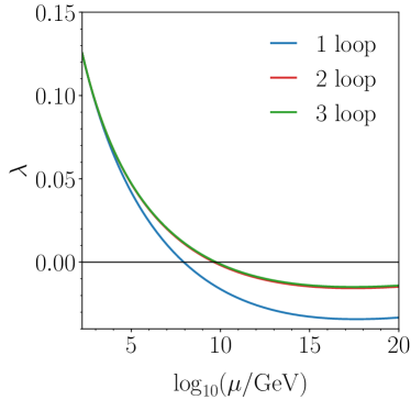
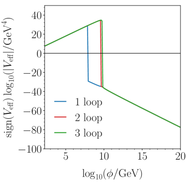
Figure 5: Left panel: RG evolution of $\lambda$ in the standard model at one, two and three loops (respectively in blue, red and green). Right panel: standard model effective potential in the approximation $V_{\rm eff}\simeq\lambda(\phi)\phi^{4}/4$.

4.5 Gauge dependence

Although the effective potential turns out to be a very useful tool for the study of spontaneous symmetry breaking, there are some subtleties related to its physical interpretation which are worth to be discussed. In particular, we are going to review here the role of the gauge dependence of the effective potential in the vacuum stability analysis and, in the next section, the so-called convexity and reality issues.

The gauge dependence of the effective potential raises the question of which are the physical observables entering the vacuum stability analysis. To fix the ideas, let us assume that all the parameters of the standard model are exactly determined, but the Higgs boson mass. After choosing the renormalization scale $\mu$, the RG improved effective potential, $V_{\rm{eff}}(\phi,M_{h};\xi)$, is a function of $\phi$, the Higgs pole mass $M_{h}$, and the gauge fixing parameters, collectively denoted by $\xi$. One can think of $M_{h}$ as an order parameter, whose variation modifies the shape of the effective potential, as sketched in Fig. 6.

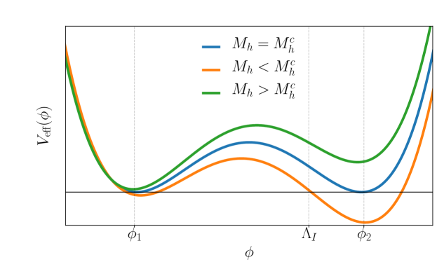
Figure 6: Schematic representation of the standard model effective potential for different values of the Higgs boson mass. For $M_{h}<M_{h}^{c}$, the electroweak vacuum is unstable.

The absolute stability bound on the Higgs boson mass is obtained by defining a “critical” mass, $M_{h}^{c}$, for which the value of the effective potential at the electroweak minimum, $\phi_{1}$, and at a second minimum, $\phi_{2}>\phi_{1}$, are the same. Analytically, this translates into the three conditions

$$V_{\rm{eff}}(\phi_{1},M_{h}^{c};\xi)-V_{\rm{eff}}(\phi_{2},M_{h}^{c};\xi)=0,$$ (4.97)

$$\left.\frac{\partial V_{\rm{eff}}}{\partial\phi}\right|_{\phi_{1},M_{h}^{c}}=\left.\frac{\partial V_{\rm{eff}}}{\partial\phi}\right|_{\phi_{2},M_{h}^{c}}=0.$$ (4.98)

We have seen in the previous section that, in the $\phi\gg\phi_{1}$ limit, the standard model effective potential is well approximated by Eq. (4.96),

$$V_{\rm{eff}}(\phi)\simeq\frac{1}{4}\lambda_{\rm{eff}}(\phi)\phi^{4}.$$ (4.99)

Hence, the absolute stability conditions in Eqs. (4.97)–(4.98) can be equivalently rewritten in the following way:

$$\lambda_{\rm{eff}}(\phi_{2},M_{h}^{c};\xi)=0,$$ (4.100)

$$\left.\frac{\partial\lambda_{\rm{eff}}}{\partial\phi}\right|_{\phi_{2},M_{h}^{c}}=0,$$ (4.101)

up to $(\phi_{1}/\phi_{2})^{2}\ll 1$ corrections.

On the other hand, due to the explicit presence of $\xi$ in the vacuum stability condition, it is not obvious a priori which are the physical (gauge-independent) observables entering the vacuum stability analysis. The basic tool, in order to capture the gauge-invariant content of the effective potential is given by the Nielsen identity [32]

$$\left(\frac{\partial}{\partial\xi}+C(\phi,\xi)\frac{\partial}{\partial\phi}\right)V_{\rm eff}(\phi,\xi)=0,$$ (4.102)

where $C(\phi,\xi)$ is a correlator involving the ghost fields and the gauge-fixing functional, whose explicit expression will not be needed for our argument. Eq. (4.102) is valid for the class of linear gauges and can be derived from the BRST non-invariance of a composite operator involving the ghost field and the gauge fixing functional (see e.g. [33]).

The identity in Eq. (4.102) has the following physical interpretation: the effective potential is gauge independent where it is stationary and hence spontaneous symmetry breaking is a gauge-invariant statement. We can actually use the Nielsen identity, in combination with the vacuum stability condition in Eqs. (4.97)–(4.98), to formally prove that the critical Higgs boson mass, $M_{h}^{c}$, is a gauge-independent quantity [34]. To this purpose, let us assume that simultaneously inverting Eqs. (4.97)–(4.98) would yield gauge dependent field values and critical Higgs boson mass: $\phi_{1}=\phi_{1}(\xi)$, $\phi_{2}=\phi_{2}(\xi)$ and $M_{h}^{c}=M_{h}^{c}(\xi)$. The total differential of Eq. (4.97) with respect to $\xi$ then reads

$$\left.\frac{\partial V_{\rm{eff}}}{\partial\phi}\right|_{\phi_{1},M_{h}^{c}}\frac{\partial\phi_{1}}{\partial\xi}+\left.\frac{\partial V_{\rm{eff}}}{\partial M_{h}}\right|_{\phi_{1},M_{h}^{c}}\frac{\partial M_{h}^{c}}{\partial\xi}+\left.\frac{\partial V_{\rm{eff}}}{\partial\xi}\right|_{\phi_{1},M_{h}^{c}}\\ =\left.\frac{\partial V_{\rm{eff}}}{\partial\phi}\right|_{\phi_{2},M_{h}^{c}}\frac{\partial\phi_{2}}{\partial\xi}+\left.\frac{\partial V_{\rm{eff}}}{\partial M_{h}}\right|_{\phi_{2},M_{h}^{c}}\frac{\partial M_{h}^{c}}{\partial\xi}+\left.\frac{\partial V_{\rm{eff}}}{\partial\xi}\right|_{\phi_{2},M_{h}^{c}}.$$ (4.103)

The first terms in both the l.h.s. and the r.h.s. of Eq. (4.103) vanish because of the stationary conditions in Eq. (4.98). The third terms in both the l.h.s. and the r.h.s. of Eq. (4.103) vanish for the same reason, after using the Nielsen identity. Hence, we are left with

$$\left(\left.\frac{\partial V_{\rm{eff}}}{\partial M_{h}}\right|_{\phi_{1},M_{h}^{c}}-\left.\frac{\partial V_{\rm{eff}}}{\partial M_{h}}\right|_{\phi_{2},M_{h}^{c}}\right)\frac{\partial M_{h}^{c}}{\partial\xi}=0.$$ (4.104)

Since the expression in the bracket of Eq. (4.104) is in general different from zero, one concludes that

$$\frac{\partial M_{h}^{c}}{\partial\xi}=0,$$ (4.105)

namely, the critical Higgs boson mass does not depend on the gauge-fixing parameters, and hence telling whether the electroweak minimum is absolutely stable or not is a physical statement. Note, however, that a non-consistent use of perturbation theory might still be responsible for a residual (spurious) gauge dependence in the determination of $M_{h}^{c}$ [35, 36].

On the other hand, field values (as for instance the instability scale) are essentially gauge-dependent quantities. The standard model vacuum instability scale is operatively defined as the field value $\phi=\Lambda_{I}$, for which the effective potential has the same depth as the electroweak minimum (see Fig. 6). This is analytically expressed by

$$V_{\rm eff}(\Lambda_{I};\xi)=V_{\rm eff}(\phi_{1};\xi).$$ (4.106)

The r.h.s. of Eq. (4.106) is a gauge-independent quantity, since $\phi_{1}$ is by definition a minimum and we can apply the Nielsen identity. Hence, by solving Eq. (4.106), one has in general $\Lambda_{I}=\Lambda_{I}(\xi)$. In particular, by taking the total differential of Eq. (4.106) with respect to $\xi$, we get

$$\left.\frac{\partial V_{\rm eff}}{\partial\phi}\right|_{\Lambda_{I}}\frac{\partial\Lambda_{I}}{\partial\xi}+\left.\frac{\partial V_{\rm eff}}{\partial\xi}\right|_{\Lambda_{I}}=0.$$ (4.107)

By using the Nielsen identity, we can substitute back the second term in Eq. (4.107), thus obtaining

$$\left(\frac{\partial\Lambda_{I}}{\partial\xi}-C(\Lambda_{I},\xi)\right)\left.\frac{\partial V_{\rm eff}}{\partial\phi}\right|_{\Lambda_{I}}=0.$$ (4.108)

Since, in general, $\Lambda_{I}$ is not an extremum of the effective potential, Eq. (4.108) yields

$$\frac{\partial\Lambda_{I}}{\partial\xi}=C(\Lambda_{I},\xi).$$ (4.109)

It turns out that by varying $\xi$ within its perturbative domain, the scale $\Lambda_{I}$ in the standard model suffers from a gauge-fixing uncertainty of up to one order of magnitude in the Fermi gauge [34]. Although $\Lambda_{I}$ is clearly unphysical, one can still identify some gauge-invariant scales related with the Higgs potential instability (see e.g. Ref. [37]).

4.6 Convexity and reality

The effective potential $V_{\rm eff}(\phi_{c})$, being defined as the Legendre transform of the generating functional of the connected Green’s functions, must be a convex function of its argument. Moreover, as we are going to show, it carries the following physical interpretation: it is the expectation value of the energy density $\langle\Psi|\mathcal{H}|\Psi\rangle$, for the lowest-energy state $|\Psi\rangle$, subject to the constraints $\langle\Psi|\Psi\rangle=1$ and $\langle\Psi|\phi(x)|\Psi\rangle=\phi_{c}$. This also implies that $V_{\rm eff}$ must be real.

These two properties of the effective potential are in apparent contrast with what done so far, since any scalar potential relevant for spontaneous symmetry breaking has non-convex regions. Moreover, the convexity and reality problems are closely related. In fact, the one-loop correction to $V_{\rm eff}$ is proportional to $[V^{\prime\prime}(\phi_{c})]^{2}\log V^{\prime\prime}(\phi_{c})$, so that non-convex regions ($V^{\prime\prime}(\phi_{c})<0$) lead to an imaginary part.

It is commonly understood that this paradox has nothing to do with the breakdown of perturbation theory, but it is rather an issue of terminology (see e.g. [38, 39, 40]). In the derivation of $V_{\rm eff}$ in Sect. 4.1 we have implicitly assumed that $\phi_{c}[J]$ (defined via the relation $\phi_{c}=\delta W/\delta J$) is a single-valued function. It can be shown that whenever the tree-level potential has non-convex regions, the relation between $\phi_{c}$ and $J$ becomes multi-valued and the standard one-loop derivation of what we improperly called the effective potential gets modified [38]. Specifically, the saddle point approximation employed in the background field method of Sect. 4.2 features multiple stationary points with respect to which the effective action should be expanded, and the true effective potential is obtained by summing over all of them.

It is therefore more appropriate to distinguish between two objects: $V_{\rm eff}$, defined in terms of the Legendre transform of the generating functional of connected Green’s functions, and $V_{\rm 1PI}$, defined as the negative of the spatially independent part of the generating functional of the 1PI Green’s functions (cf. Eq. (4.14)). The two generating functionals are related by (see e.g. [41])

$$\exp{\left[\frac{i}{\hbar}\left(W[J]+\mathcal{O}(\hbar)\right)\right]}=\mathcal{N}\int\mathcal{D}\phi_{c}\exp{\left[\frac{i}{\hbar}\left(\Gamma_{\rm 1PI}[\phi_{c}]+\int d^{4}x\,J(x)\phi_{c}(x)\right)\right]},$$ (4.110)

for some irrelevant normalization constant $\mathcal{N}$. In the semi-classical limit, $\hbar\to 0$, we can use the saddle point approximation to obtain

$$W[J]=\left.\left[\Gamma_{\rm 1PI}[\phi_{c}]+\int d^{4}x\,J(x)\phi_{c}(x)\right]\right|_{\frac{\delta\Gamma_{\rm 1PI}}{\delta\phi_{c}}=-J}.$$ (4.111)

Hence, $W[J]$ is the Legendre transform of $\Gamma_{\rm 1PI}[\phi_{c}]$. On the other hand, the effective action was defined as the Legendre transform of $W[J]$

$$\Gamma_{\rm eff}[\phi_{c}]=\left.\left[W[J]-\int d^{4}x\,J(x)\phi_{c}(x)\right]\right|_{\frac{\delta W}{\delta J}=\phi_{c}}.$$ (4.112)

Therefore $\Gamma_{\rm eff}[\phi_{c}]$ is the double Legendre transform of $\Gamma_{\rm 1PI}[\phi_{c}]$. From the properties of Legendre transforms it follows that $\Gamma_{\rm eff}[\phi_{c}]$ is the convex envelope of $\Gamma_{\rm 1PI}[\phi_{c}]$. In turn, this implies that $V_{\rm eff}$ is the convex envelope of $V_{\rm 1PI}$.

Note that the formalism behind $V_{\rm eff}$ is defined in the thermodynamical limit, where the system has relaxed on the ground state after an infinite amount of time. On the other hand, in most applications, we are rather interested in metastable regimes described by field configurations localized around a local minimum. The goal of this section is to show that $V_{\rm 1PI}$ is actually the appropriate object in order to describe this physical situation.

Following Coleman [10], we start by considering the quantum mechanical problem of constructing a state $|a\rangle$ that is a stationary state of the quadratic form $\langle a|H|a\rangle$, subject to the constraints $\langle a|a\rangle=1$ and $\langle a|A|a\rangle=A_{c}$, for some Hermitian operator $A$. This can be cast in the variational problem $\delta\langle a|H-E-JA|a\rangle=0$, where $E$ and $J$ are Lagrangian multipliers. The variational equation leads to

$$[H-E-JA]|a\rangle=0,$$ (4.113)

from which we see that $|a\rangle$ is an eigenstate of the perturbed Hamiltonian $H-JA$, with energy $E$. Eq. (4.113) allows us to express $|a\rangle=|a(E,J)\rangle$ and, further using the normalization condition, we can express $E$ in terms of $J$. Since we are eventually interested in the dependence on $A_{c}$, the relation between $J$ and $A_{c}$ can be obtained via standard perturbation theory

$$A_{c}(J)=\langle a(J)|A|a(J)\rangle=-\frac{dE}{dJ}.$$ (4.114)

Hence, we conclude that $|a\rangle$ is the stationary state of the quantity

$$\langle a(J)|H|a(J)\rangle=E(J)+JA_{c}=E(J)-J\frac{dE}{dJ}.$$ (4.115)

The generalization to quantum field theory is obtained by replacing: $|a\rangle\to|\Psi\rangle$, $H\to\mathcal{H}$, $A\to\phi$, $A_{c}\to\phi_{c}$, $E\to W$, which corresponds to the definition of the effective action in Eq. (4.112). Hence, we conclude that

$$V_{\rm eff}(\phi_{c})=\langle\Psi|\mathcal{H}|\Psi\rangle,$$ (4.116)

for a state $|\Psi\rangle$ such that $\delta\langle\Psi|\mathcal{H}|\Psi\rangle=0$, under the constraints $\langle\Psi|\Psi\rangle=1$ and $\langle\Psi|\phi(x)|\Psi\rangle=\phi_{c}$.

To investigate this further, let us consider for definiteness the case of the double-well potential $V(\phi)=-\frac{1}{2}\mu^{2}\phi^{2}+\frac{1}{4}\lambda\phi^{4}$ with minima in $\phi=\pm\sigma\equiv\sqrt{\mu^{2}/\lambda}$ (cf. Fig. 7).

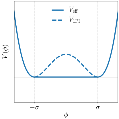
Figure 7: Example of a non-convex tree-level potential. The true effective potential ($V_{\rm eff}$) is the convex envelope of $V_{\rm 1PI}$.

The classical potential is clearly non-convex in the region $\phi<\left|\sigma\right|$. Following Weinberg and Wu [42], the main features of the effective potential can be understood via a classical argument. Let us consider the classical analog of $\langle\Psi|\phi(x)|\Psi\rangle$ to be the spatial average of $\phi$, denoted by $\overline{\phi}$. Using the physical interpretation of the effective potential, the classical analog of the effective potential, $V_{c}$, is the minimum value of the energy density among all the states with a given value of $\overline{\phi}$. For $\phi>|\sigma|$ the energy density

$$\mathcal{H}=\frac{1}{2}\dot{\phi}^{2}+\frac{1}{2}(\bm{\nabla}\phi)^{2}+V(\phi),$$ (4.117)

is mimimized by a static homogeneous configuration with $\phi(x)=\overline{\phi}$ everywhere, and $V_{c}$ is equal to $V(\phi)$. If $\phi<|\sigma|$, there is a non-trivial way in which the energy density can be minimized, namely via an inhomogeneous state

$$\phi(x)=\left\{\begin{array}[]{l}+\sigma\quad\text{for a fraction $f$ of space}\\ -\sigma\quad\text{otherwise}\end{array}\right.$$ (4.118)

where $0\leq f\leq 1$ is fixed by requiring that the spatial average of $\phi(x)$, $\sigma f-\sigma(1-f)$, is equal to $\overline{\phi}$, which yields $f=(\overline{\phi}+\sigma)/(2\sigma)$. Hence, in the $\phi<|\sigma|$ region the energy density is $V(\pm\sigma)<V(\phi)$. Note that the gradient term relevant at the boundaries of the two domains can be neglected in the infinite volume limit. $V_{c}$ is thus flat in the region between the two minima, and corresponds to the convex envelop of the $V(\phi)$. In the quantum theory, the main difference is that the state which minimizes the energy density is not a spatially inhomogeneous mixture of two phases but rather a quantum superposition of two vacuum states.

If one is interested only in homogeneous states, i.e. states in which the field is concentrated about a specific value, then the effective potential is not the appropriate quantity to describe the region $\phi<|\sigma|$. In that case one would need a modified effective potential which might be defined as the expectation value of the energy density in a state $|\Psi\rangle$ which minimizes $\langle\Psi|\mathcal{H}|\Psi\rangle$ subject to the condition $\langle\Psi|\phi(x)|\Psi\rangle=\phi_{c}$ and to the further restriction that the wave functional for $|\Psi\rangle$ be concentrated on configurations with $\phi(x)\approx\phi_{c}$. Hence, to leading order the minimum energy density is $V(\phi_{c})$ which does not need to be convex. Zero point fluctuations are further taken into account by $V_{\rm 1PI}(\phi_{c})$, whose real part provides the relevant potential to address localized field configurations prior to a phase transition. Note that the restriction to localized configurations does not commute with the Hamiltonian (e.g. in the case if the double-well potential the energy eigenstates are even/odd linear combinations of the states localized in $\pm\sigma$), thus these configurations are unstable and can be interpreted as imaginary contributions to the energy [42]. This instability, related to the imaginary part of the perturbatively computed $V_{\rm 1PI}$, should not to be confused with the non-perturbative decay of the false vacuum itself (for instance, one could consider a non-convex $V_{\rm 1PI}$ with field configurations localized around the true vacuum).

Following a standard terminology, we will keep to refer to $V_{\rm eff}$ as the (localized) effective potential.

5 Decay of the standard model vacuum

The stability of the electroweak ground state is a time-honoured subject [43, 44, 45, 46, 47, 48, 49, 50, 40, 51, 52]. Prior to the Higgs discovery in 2012 [53, 54] it served as a theoretical tool to set a lower bound on the Higgs boson mass [55, 56, 57, 58, 3, 59, 60]. Recently, the analysis of the standard model vacuum stability has reached a higher level of complexity (see e.g. [61, 62, 63, 31, 64, 65, 66, 67]). In this section we describe the basic aspects of the calculation of the standard model vacuum decay rate and we introduce the so-called standard model phase diagram, namely the parameter space region in the standard model for which the electroweak vacuum is absolutely stable, metastable (i.e. with a sufficiently long lifetime compared to the age of the Universe) or worryingly unstable.

5.1 The origin of the standard model instability

The case of the standard model of electroweak interactions is different from the simple examples described in Sect. 3. Indeed, the tree-level scalar potential of the standard model

$$V_{0}(\phi)=\frac{1}{2}m^{2}\phi^{2}+\frac{1}{4}\lambda\phi^{4}$$ (5.1)

with $m^{2}<0$ and $\lambda>0$ has a local maximum at $\phi=0$, an absolute minimum at $\phi=\sqrt{-\frac{m^{2}}{\lambda}}=v$ (the electroweak minimum), with $v\sim 246$ GeV, and no other stationary points. Hence, at the classical level, there is no instability of the ground state.

The situation changes when loop corrections are included. As we have seen in the previous section, the effective potential behaves as $\lambda(\phi)\phi^{4}$ for large values of the classical field $\phi$, and the running coupling $\lambda(\mu)$ becomes negative at $\mu=\Lambda_{I}\sim 10^{10}$ GeV if the top quark is sufficiently heavy. If this is the case, the electroweak minimum is not the absolute minimum of the effective potential: a second, deeper minimum, located somewhere between $10^{10}$ GeV and the position of the Landau singularity, must therefore exist, and quantum fluctuations may induce tunnelling from the electroweak minimum to the absolute minimum.

The study of the instability of the electroweak ground state must therefore be carried on consistently at the level of loop corrections.

Since such large energy scales and field values are involved, the calculation of the tunnelling probability is in general influenced by the ultraviolet completion of the standard model (if any), and by gravitational effects; it is however reasonable to take a conservative point of view, and perform a calculation of the false vacuum lifetime under the assumption that the standard model is a correct description of our Universe up to scales of the order of the Planck mass.

5.2 The standard model bounce

We have seen in Sect. 3 that the calculation of the decay rate of an unstable ground state in quantum field theory is based on an $\,{\rm O}(4)$-invariant bounce, $\phi(x)=\phi_{b}(r)$, solution of the field equation

$$\phi^{\prime\prime}_{b}(r)+\frac{3}{r}\phi_{b}^{\prime}(r)=V^{\prime}(\phi_{b})$$ (5.2)

where $V(\phi)$ is the scalar potential expressed in terms of renormalized parameters, with boundary conditions

$$\lim_{r\to\infty}\phi_{b}(r) =v,$$ (5.3)

$$\phi_{b}^{\prime}(0) =0.$$ (5.4)

In the case of the standard model the value of $\phi$ (which denotes the Higgs background field, see Eqs. (4.36)–(4.37)) at the true minimum of the scalar potential is typically many orders of magnitudes larger that the electroweak order parameter, $v\sim 246$ GeV. It seems therefore appropriate to simply neglect the finite value of $v$ with respect to the typical energy scales involved in the problem of the quantum stability of the electroweak ground state. We will therefore adopt the boundary condition

$$\lim_{r\to\infty}\phi_{b}(r)=0,$$ (5.5)

and we will approximate the scalar potential in the unstable region by

$$V(\phi)=\frac{1}{4}\lambda(\phi)\phi^{4},$$ (5.6)

with the renormalized coupling $\lambda(\mu)$ computed at a scale $\mu\sim\phi$ to reduce the impact of large logarithms. Eq. (5.2) takes the form

$$\phi^{\prime\prime}_{b}+\frac{3}{r}\phi^{\prime}_{b}=\phi_{b}^{3}\left[\lambda(\phi_{b})+\frac{1}{4}\beta(\lambda(\phi_{b}))\right],$$ (5.7)

where

$$\beta(\lambda(\mu))=\mu\frac{d\lambda(\mu)}{d\mu}.$$ (5.8)

(Although not explicitly indicated, the function $\beta(\lambda)$ actually depends on all coupling constants in the theory, and in particular on the top Yukawa coupling, which drives $\lambda$ to negative values, as we have seen in Sect. 4.) A bounce solution of Eq. (5.7), that is, a solution with $\phi^{\prime}_{b}(0)=\phi_{b}(\infty)=0$, certainly exists, because the scalar potential Eq. (5.6) has a local minimum in $\phi=0$ and an absolute minimum at some very large value of $\phi$, and the undershoot-overshoot argument of Sect. 3.2 can be applied. We recall that, by the same argument, the value of the bounce at $r=0$ is larger than the position of the first zero of $\lambda(\mu)$, $\mu\sim\Lambda_{I}=10^{10}$ GeV. At such large values of the classical field, the use of the approximation (5.6) is largely justified; the mass term would induce a correction

$$\frac{\Delta\phi(0)}{\phi(0)}<\frac{v}{\Lambda_{I}}\sim 10^{-8}.$$ (5.9)

An analytic solution of Eq. (5.7) cannot be found. However, it can be checked that the dependence of the combination

$$\lambda(\phi)+\frac{1}{4}\beta(\lambda(\phi))$$ (5.10)

on $\phi$ in the region where $\lambda(\phi)<0$ is very weak: it is only logarithmic, and it is suppressed by powers of the coupling constants. An approximate solution can therefore be found by replacing the r.h.s. of Eq. (5.7) by a negative constant $\lambda$. As we are going to show below, a good approximation is obtained by fixing $\lambda=\lambda(\overline{\mu})$ where $\overline{\mu}$ is such that $\beta(\lambda(\overline{\mu}))=0$. Eq. (5.7) then becomes

$$\phi^{\prime\prime}_{b}(r)+\frac{3}{r}\phi^{\prime}_{b}(r)=\lambda\phi_{b}^{3}(r).$$ (5.11)

(Incidentally, we note that we are now precisely in the situation described in Sect. 3.4, namely a scalar potential with no barrier.) As anticipated in Sect. 3.5.1 and shown explicitly in App. A.5, Eq. (5.11) with the boundary conditions (5.4, 5.5) can be solved analytically. There is in fact an infinity of solutions:

$$\phi_{b}(r)=\frac{\phi_{b}(0)}{1+\frac{|\lambda|}{8}\phi_{b}^{2}(0)r^{2}},$$ (5.12)

parametrized by $\phi_{b}(0)$, which can take any positive value. Eq. (5.12) is often rewritten in terms of a length scale $R$, rather than by its value at $r=0$:

$$\phi_{b}(r)=\sqrt{\frac{8}{|\lambda|}}\frac{R}{r^{2}+R^{2}}.$$ (5.13)

The parameter $R$ can be physically interpreted as the approximate radius of the bubble, in three dimensional space, where the system has jumped from the false-vacuum configuration $\phi_{b}=0$ to a non-zero value beyond the barrier. Indeed, $\phi_{b}(r)$ has its maximum in $r=0$:

$$\phi_{b}(0)=\sqrt{\frac{8}{|\lambda|}}\frac{1}{R},$$ (5.14)

and drops to zero for $r\gg R$. Note that $\phi_{b}(R)=\frac{\phi_{b}(0)}{2}$, which justifies our definition of $R$ as the radius of the bubble.

As already noted in Sect. 3.5.1, this degeneracy is a consequence of scale invariance. Indeed, the underlying action functional

$$S[\phi]=\int d^{4}x\,\left[\frac{1}{2}(\partial_{\mu}\phi)^{2}+\frac{1}{4}\lambda\phi^{4}\right]$$ (5.15)

is invariant upon scale transformations:

$$\phi(r)\to a\phi(ar),$$ (5.16)

since it does not contain any dimensionful parameter. The proof is straightforward:

$$S[a\phi(ar)]=\int d^{4}x\,\left[\frac{a^{2}}{2}\left(\frac{\partial\phi(ar)}{\partial x_{\mu}}\right)^{2}+\frac{a^{4}}{4}\lambda\phi^{4}(ar)\right]=S[\phi]$$ (5.17)

after the integration variable change $y=ax$. As a consequence, if $\phi(r)$ is a solution of Eq. (5.11), than $a\phi(ar)$ is also a solution, for any choice of the scale factor $a$:

$$\left(\frac{d^{2}}{dr^{2}}+\frac{3}{r}\frac{d}{dr}\right)[a\phi(ar)]=a^{3}\left[\phi^{\prime\prime}(ar)+\frac{3}{ar}\phi^{\prime}(ar)\right]=\lambda[a\phi(ar)]^{3}.$$ (5.18)

The transformation $\phi(r)\to a\phi(ar)$ on Eq. (5.12) amounts to rescaling

$$\phi_{b}(0)\to a\phi_{b}(0).$$ (5.19)

However, the scale invariance of Eq. (5.11) is not a feature of our original problem, but rather a consequence of our approximations. The original field equation, Eq. (5.7), is not scale-invariant, even when mass terms are neglected, because of renormalization; therefore, its bounce solution has a definite value at $r=0$. Unfortunately, the correct value of $\phi_{b}(0)$ cannot be determined analytically. A numerical study of the bounce solution to Eq. (5.7) was presented for instance in Ref. [20] based on the shooting method reviewed in App. A.6. The results show that the commonly adopted approximation in Eq. (5.11) is rather accurate. However, its application in the calculation of the first quantum corrections requires some care, as discussed below in Sect. 5.4.

We conclude this section by computing the action of the Fubini-Lipatov bounces Eq. (5.12), which enters the calculation of the decay rate of the metastable ground state. The action is easily computed using Eq. (3.12):

$$S[\phi_{b}]=-\int d^{4}x\,V(\phi_{b}(x))=-2\pi^{2}\int_{0}^{+\infty}dr\,r^{3}V(\phi_{b}(r)),$$ (5.20)

where in the last step we have used the $\,{\rm O}(4)$ invariance of the bounce solution. We find

$$S[\phi_{b}]=\frac{8\pi^{2}}{3|\lambda|},$$ (5.21)

independently of the value of $\phi_{b}(0)$, as expected.

5.3 A digression on scale transformations

In this section we collect some considerations about the role of scale invariance (or non-invariance) in the search for bounce solutions of the field equations. Let us consider a generic scalar field theory, with scalar potential $V(\phi)$, and let us assume that the action $S[\phi]$ is stationary around $\phi=\phi_{b}$. Then, in particular, it will be stationary upon infinitesimal scale transformations, that is we expect

$$\Delta B=\Delta\left(S[\phi_{b}]-S[\phi_{\rm FV}]\right)=0$$ (5.22)

upon a variation

$$\Delta\phi=(1+x_{\rho}\partial_{\rho})\phi_{b}$$ (5.23)

around a solution of the field equation. A straightforward calculation gives

$$\Delta B=\int d^{4}x\,\left[\phi V^{\prime}(\phi_{b})-4V(\phi_{b})+4V(\phi_{\rm FV})\right].$$ (5.24)

The r.h.s. of Eq. (5.24) is obviously zero for

$$V(\phi)=\frac{1}{4}\lambda\phi^{4}+V(\phi_{\rm FV}),$$ (5.25)

because the integrand vanishes identically in this case. We already know that in this case bounce solutions of the field equation exist if $\lambda<0$.

It is easy to find examples of scalar potentials that do not admit any bounce solution of the field equation. Consider for instance

$$V(\phi)=\frac{1}{4}\lambda\phi^{4}+\frac{1}{2}m^{2}\phi^{2}$$ (5.26)

with $\lambda<0$ and constant $m^{2}$, either positive or negative. In this case,

$$\Delta B=\Delta S[\phi]=-m^{2}\int d^{4}x\,\phi^{2}(x),$$ (5.27)

which vanishes only for $\phi(x)=0$.

There are however intermediate cases, that is, non-scale-invariant scalar potentials that admit a bounce solution of the field equation. For example

$$V(\phi)=g\left[\frac{1}{4}\phi^{4}-\frac{1}{3}\phi^{3}(M+\phi_{\rm TV})+\frac{1}{2}\phi^{2}M\phi_{\rm TV}\right]$$ (5.28)

with $g>0$ and

$$0<M<\frac{\phi_{\rm TV}}{2}$$ (5.29)

has a local minimum for $\phi=0$ and an absolute minimum for $\phi=\phi_{\rm TV}$, separated by a barrier with its maximum for $\phi=M$. A plot of $\frac{V(\phi)}{g\phi_{\rm TV}^{4}}$ as a function of $h=\frac{\phi}{\phi_{\rm TV}}$ for different values of $m=\frac{M}{\phi_{\rm TV}}$ is shown in Fig. 8.

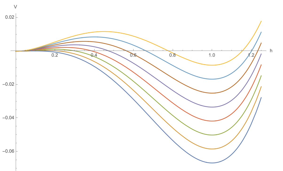
Figure 8: The scalar potential Eq. (5.28), normalized to $g\phi_{\rm TV}^{4}$, for different values of $m$. From top to bottom, $m=0.45,0.4,0.35,0.3,0.25,0.2,0.15,0.1$.

In this case the field equation

$$\phi^{\prime\prime}+\frac{3}{r}\phi^{\prime}=g\phi(\phi-M)(\phi-\phi_{\rm TV})$$ (5.30)

cannot be solved analytically. We know, however, that it must have a bounce solution, as a consequence of the overshoot-undershoot argument illustrated in Sect. 3.2. It is possible to solve the field equation numerically; the bounce $h(x)$ as a function of $x=\sqrt{g}\phi_{\rm TV}r$ is plotted in Fig. 9 for different values of $m$.

Figure 9: Bounce solutions relative to the scalar potential in Eq. (5.28) for different values of $m$.

Note that $h(0)$ gets close to 1, i.e. $\phi(0)$ close to $\phi_{\rm TV}$, as $m\to\frac{1}{2}$, where the two minima are degenerate. Also note that the solution is unique, as a consequence of the explicit breaking of scale invariance, contrary to what happens for the scale-invariant potential Eq. (5.25): the condition

$$\Delta B=g\int d^{4}x\,\left[\frac{1}{3}\phi_{b}^{3}(M+\phi_{\rm TV})-\phi_{b}^{2}M\phi_{\rm TV}\right]=0$$ (5.31)

fixes the value of the bounce at $r=0$. It can be shown that in this case the bounce is well approximated by a gaussian

$$\phi_{b}(r)=\phi_{0}e^{-\frac{r^{2}}{R^{2}}},$$ (5.32)

in the sense that values of the parameters $\phi_{0}$ and $R$ can be found, such that the true bounce action is accurately reproduced.

The standard model scalar potential with the mass term neglected and the running coupling computed at $\mu\sim\phi$,

$$V(\phi)=\frac{1}{4}\lambda(\phi)\phi^{4};\qquad\mu\frac{d\lambda}{d\mu}=\beta(\lambda)$$ (5.33)

also belongs to the same class: it has a local minimum at $\phi=0$, increases with $\phi$, then starts decreasing when $\lambda(\phi)$ becomes negative. We have argued in the previous section that in this case the bounce is well approximated by the Fubini-Lipatov bounce; the value of $\phi(0)$ is determined by the condition of stationarity of the action upon scale transformations,

$$\Delta B=\frac{1}{4}\int d^{4}x\,\beta(\lambda(\phi_{b}))\phi_{b}^{4}=0.$$ (5.34)

An analytical estimate of $\phi_{b}(0)$ in this case is presented in Ref. [68]: for values of $\phi$ not too far from the value of the scale $\overline{\mu}$ where $\lambda(\overline{\mu})$ has a minimum we have

$$\lambda(\phi)=\lambda(\overline{\mu})+\frac{1}{2}\left.\frac{d\beta(\lambda(\phi))}{d\log\phi}\right|_{\phi=\overline{\mu}}\log^{2}\frac{\phi}{\overline{\mu}}+O\left(\log^{3}\frac{\phi}{\overline{\mu}}\right)$$ (5.35)

and therefore

$$\beta(\lambda(\phi))=\left.\frac{d\beta(\lambda(\phi))}{d\log\phi}\right|_{\phi=\overline{\mu}}\log\frac{\phi}{\overline{\mu}}+O\left(\log^{2}\frac{\phi}{\overline{\mu}}\right).$$ (5.36)

Neglecting terms of order $\log^{2}\frac{\phi}{\overline{\mu}}$, the stationarity condition in Eq. (5.34) yields

$$\int d^{4}x\,\phi_{b}^{4}(r)\log\phi_{b}(r)=\log\overline{\mu}\int d^{4}x\,\phi_{b}^{4}(r).$$ (5.37)

The two integrals are easily computed with $\phi(r)$ replaced by the Fubini-Lipatov bounce Eq. (5.12). We get

$$\log\frac{\phi_{b}(0)}{\overline{\mu}}\int\frac{r^{3}dr}{\left(1+\frac{|\lambda|}{8}\phi^{2}_{b}(0)r^{2}\right)^{4}}=\int\frac{r^{3}dr}{\left(1+\frac{|\lambda|}{8}\phi_{b}^{2}(0)r^{2}\right)^{4}}\log\left(1+\frac{|\lambda|}{8}\phi_{b}^{2}(0)r^{2}\right)$$ (5.38)

or

$$\phi_{b}(0)=\overline{\mu}e^{\frac{5}{6}}.$$ (5.39)

The result in Eq. (5.39) can be turned into an estimate of the bounce size $R$, defined by Eq. (5.14). We obtain

$$R=\sqrt{\frac{8}{|\lambda(\overline{\mu})|}}\frac{1}{\phi_{b}(0)}\sim\frac{10}{\overline{\mu}}$$ (5.40)

for $|\lambda(\overline{\mu})|\sim 0.013$. Because $\overline{\mu}\sim 10^{17}$ GeV, Eq. (5.39) is an a-posteriori confirmation that the mass term in the potential can be safely neglected.

For earlier work discussing the breaking of scale invariance due to the running of $\lambda$ in the context of the standard model vacuum tunnelling calculation see also Refs. [51, 52].

5.4 First quantum corrections

The calculation of the first quantum corrections to the decay rate of the standard model vacuum is presented in Ref. [3]. The calculation is performed by the procedure illustrated in Sect. 3.5, which produces the result

$$\frac{\gamma}{{\mathcal{V}}_{3}}=\frac{\left(S[\phi_{b}]-S[\phi_{\rm FV}]\right)^{2}}{(2\pi)^{2}}\sqrt{\frac{\mbox{Det}\,S^{\prime\prime}[\phi_{\rm FV}]}{|\mbox{Det}\,^{\prime}S^{\prime\prime}[\phi_{b}]|}}e^{-\left(S[\phi_{b}]-S[\phi_{\rm FV}]\right)}e^{-\left(S_{\rm ct}[\phi_{b}]-S_{\rm ct}[\phi_{\rm FV}]\right)},$$ (5.41)

for the decay rate per unit volume of the metastable ground state.

In the case of the standard model, the calculation of the pre-exponential factor is complicated by the presence of fermion and vector degrees of freedom in the theory, which contribute fluctuations around the bounce configuration. We will not reproduce here the full calculation; we limit ourselves to pointing out a few important features.

The first point is the choice of a suitable basis for the space of eigenfunctions of $S^{\prime\prime}[\phi]$ for the evaluation of ratios of functional determinants

$$\frac{\mbox{Det}\,S^{\prime\prime}[\phi_{b}]}{\mbox{Det}\,S^{\prime\prime}[\phi_{\rm FV}]}.$$ (5.42)

This requires solving eigenvalue equations of the type

$$S^{\prime\prime}[\phi]\,u=[-\partial^{2}+W(\phi)]u=\lambda u,$$ (5.43)

where $u$ generically denotes scalar, fermion or gauge fields, and the function $W(\phi)$ takes different forms for each contribution.

Because $W(\phi)$ in (5.43) depends only on the radial coordinate $r$, it is convenient to decompose the various fields in eigenstates of the four-dimensional angular momentum operator $L^{2}=L_{\mu\nu}L_{\mu\nu}$, where

$$L_{\mu\nu}=\frac{i}{\sqrt{2}}\left(x_{\mu}\partial_{\nu}-x_{\nu}\partial_{\mu}\right).$$ (5.44)

The Laplace operator takes the form

$$\partial^{2}=\partial_{\mu}\partial_{\mu}=\frac{d^{2}}{dr^{2}}+\frac{3}{r}\frac{d}{dr}-\frac{L^{2}}{r^{2}}.$$ (5.45)

In the case of scalar fields, the eigenfunctions of $L^{2}$ are the four-dimensional spherical harmonics $Y_{j}(\theta)$ (where $\theta$ collectively denotes the 3 polar angles) with eigenvalues $4j(j+1)$, and degeneracy $(2j+1)^{2}$, where $j$ takes integer and semi-integer values. In this basis, $S^{\prime\prime}[\phi_{b}]$ is block-diagonal, with blocks $\left(S^{\prime\prime}[\phi_{b}]\right)_{j}$ labelled by $j$; therefore

$$\log\mbox{Det}\,S^{\prime\prime}[\phi_{b}]=\sum_{j}\log\mbox{Det}\,(S^{\prime\prime}[\phi_{b}])_{j}.$$ (5.46)

The situation is slightly more complicated for fermion and vector fields; details can be found in Ref. [3].

As illustrated in Sect. 2.2.2, in order to compute the ratio in Eq. (5.42) it is only necessary to solve Eq. (5.43) for $\lambda=0$:

$$\rho_{j}\equiv\frac{\mbox{Det}\,\left[-\partial^{2}+W(\phi_{b})\right]}{\mbox{Det}\,\left[-\partial^{2}+W(\phi_{\rm FV})\right]}=\lim_{r\to\infty}\frac{\mbox{det}\,u^{j}_{\phi_{b}}(r)}{\mbox{det}\,u^{j}_{\phi_{\rm FV}}(r)},$$ (5.47)

where $u^{j}_{\phi}(r)$ are solutions of

$$[-\partial^{2}+W(\phi)]\,u^{j}_{\phi}(r)=0.$$ (5.48)

The symbol det in Eq. (5.47) stands for the ordinary determinant over residual (spinorial, gauge group, etc.) indices of these solutions.

The second important point is the subtraction of ultraviolet divergences. The ultraviolet behaviour of the functional determinant is encoded in the behaviour of the determinants for $j\to\infty$; as a consequence, the sum over $j$ in Eq. (5.46) is not convergent, and the usual renormalization procedure is needed. The counterterm action $S_{\rm ct}$ removes the ultraviolet divergences that arise in the calculation of the functional determinants. Indeed,

$$\sqrt{\mbox{Det}\,S^{\prime\prime}[\phi]}e^{S[\phi]+S_{\rm ct}[\phi]}=e^{S[\phi]+S_{\rm ct}[\phi]+\frac{1}{2}\log{\rm Det}\,S^{\prime\prime}[\phi]}=e^{\Gamma[\phi]},$$ (5.49)

where $\Gamma[\phi]$ is the one-loop effective action, defined in Sect. 4. For example, in the $\overline{\rm MS}$ scheme (dimensional regularization with $\overline{\rm MS}$ subtraction) the renormalized one-loop action can be written as

$$\Gamma[\phi]=S^{\overline{\rm MS}}[\phi]+\left[\Delta S[\phi]-\left(\Delta S[\phi]\right)_{\rm pole}\right],$$ (5.50)

where $S^{\overline{\rm MS}}[\phi]$ is the lowest-order action expressed in terms of the renormalized $\overline{\rm MS}$ couplings, and $\left(\Delta S\right)_{\rm pole}$ is the divergent part of $\Delta S$ defined according to the $\overline{\rm MS}$ renormalization prescription. The calculation of the full determinant in $d=4-2\epsilon$ dimensions can be avoided by observing that the ultraviolet divergences are all contained in $\Delta S^{[2]}$, defined as the expansion of $\Delta S$ up to second order in $W$:

$$\Delta S^{[2]}[\phi]=\frac{1}{2}\left[\log\mbox{SDet}\,\left(-\partial^{2}+W(\phi)\right)\right]_{O(W^{2})},$$ (5.51)

where ${\rm SDet}\,O={\rm Det}\,O$ or ${\rm SDet}\,O=({\rm Det}\,O)^{-2}$ depending on whether the operator $O$ acts on boson or fermion fields. This is easily seen in the case of scalar degrees of freedom, when

$$W_{\rm scalar}(\phi)=V^{\prime\prime}(\phi).$$ (5.52)

In renormalizable theories, the second derivative of the scalar potential is a polynomial of degree 2 in the field, while counterterms are a polynomial of degree 4. Hence the difference $\Delta S-\Delta S^{[2]}$ is ultraviolet-finite. Eq. (5.50) can be rewritten as

$$\Gamma[\phi]=S^{\overline{\rm MS}}[\phi]+\bigg{[}\Delta S[\phi]-\Delta S^{[2]}[\phi]\bigg{]}+\bigg{[}\Delta S^{[2]}[\phi]-\left(\Delta S[\phi]\right)_{\rm pole}\bigg{]},$$ (5.53)

where the two terms in square brackets are separately finite. The advantage of this last expression is that $\Delta S^{[2]}[\phi]$ can be computed either as a (divergent) sum of terms corresponding to different values of the angular momentum, which gives a finite result when subtracted from $\Delta S[\phi]$, or by standard diagrammatic techniques in $4-2\epsilon$ dimensions.

The details of the calculation of one-loop contributions to $\Gamma[\phi_{b}]$ from field fluctuations in the different sectors of the theory described in Ref. [3] is performed in terms of the Fubini-Lipatov bounce, Eq. (5.12) or Eq. (5.13), with $\phi_{b}(0)$, or equivalently $R$, fixed as described at the end of Sect. 5.3. In this approximation, the zero mode of scale invariance in the scalar sector is not normalizable, as shown Sect. 3.5.1. This is however an artifact of our approximations: the bounce is a solution of Eq. (5.11), rather than Eq. (5.7). This difficulty is overcome by removing the zero eigenvalue of dilatations from the functional determinant, and replacing it by a slightly negative eigenvalue, induced by radiative corrections.

Additional zero modes of $S^{\prime\prime}[\phi_{b}]$ arise because of the gauge symmetry; the corresponding contributions to the path integral must be removed and replaced by an integration over suitable collective coordinates. This procedure is described in Ref. [17], and involves a jacobian factor proportional to

$$\int d^{4}x\,\phi_{b}^{2}(r)$$ (5.54)

(see Eq. (3.62)), which is infrared divergent in the case of the Fubini-Lipatov bounce. Again, this is a consequence of our approximation of neglecting mass terms, and hence the nonvanishing vacuum expectation value of the Higgs field, in the scalar potential; in the real world, the Higgs mass acts as a regulator of the infrared divergence of Eq. (5.54). To see how this works we consider the field equation

$$\phi^{\prime\prime}_{b}(r)+\frac{3}{r}\phi^{\prime}_{b}(r)=V^{\prime}(\phi_{b})$$ (5.55)

in the large-$r$ limit. In this region, $\phi_{b}(r)\to\phi_{\rm FV}$, which is different from zero if the mass term is not neglected. In this limit, the field equation can be linearized by expanding the scalar potential in powers of $\phi_{b}-\phi_{\rm FV}$:

$$V(\phi_{b})=V(\phi_{\rm FV})+\frac{1}{2}V^{\prime\prime}(\phi_{\rm FV})(\phi_{b}-\phi_{\rm FV})^{2}+\,{\rm O}\left((\phi_{b}-\phi_{\rm FV})^{3}\right),$$ (5.56)

where $V^{\prime\prime}(\phi_{\rm FV})=m^{2}$ is a positive constant, related to the physical Higgs squared mass. Neglecting terms of order $(\phi_{b}-\phi_{\rm FV})^{3}$, Eq. (5.55) becomes

$$(\phi_{b}(r)-\phi_{\rm FV})^{\prime\prime}+\frac{3}{r}(\phi_{b}(r)-\phi_{\rm FV})^{\prime}=m^{2}(\phi_{b}(r)-\phi_{\rm FV}),$$ (5.57)

and can be solved analytically. In terms of the dimensionless quantities

$$x=rm;\qquad f(x)=r(\phi_{b}(r)-\phi_{\rm FV})$$ (5.58)

Eq. (5.57) reads

$$x^{2}f^{\prime\prime}(x)+xf^{\prime}(x)-(1+x^{2})f(x)=0,$$ (5.59)

which is solved by a linear combination of modified Bessel functions

$$f(x)=\alpha K_{1}(x)+\beta I_{1}(x),$$ (5.60)

where

$$I_{1}(x) =\frac{x}{2}\sum_{n=0}^{\infty}\frac{1}{n!(n+1)!}\left(\frac{x^{2}}{4}\right)^{n}$$ (5.61)

$$K_{1}(x) =\left(\log\frac{x}{2}+\gamma\right)I_{1}(x)+\frac{1}{x}+\frac{x}{4}\sum_{n=0}^{\infty}\frac{1}{n!(n+1)!}\left(\sum_{k=1}^{n+1}\frac{1}{k}+\sum_{k=1}^{n}\frac{1}{k}\right)\left(\frac{x^{2}}{4}\right)^{n}.$$ (5.62)

The large-$x$ behaviors of $I_{1}(x),K_{1}(x)$ are as follows:

$$I_{1}(x) \sim\frac{1}{\sqrt{2\pi x}}e^{x}$$ (5.63)

$$K_{1}(x) \sim\sqrt{\frac{\pi}{x}}e^{-x}.$$ (5.64)

The condition $\phi_{b}(r)-\phi_{\rm FV}\to 0$ for $r\to\infty$ gives $\beta=0$, and therefore in this limit

$$\phi_{b}(r)-\phi_{\rm FV}\simeq\alpha m\frac{K_{1}(rm)}{rm}\sim\frac{1}{(rm)^{3/2}}e^{-rm}.$$ (5.65)

This shows that $\phi^{2}_{b}(r)$ is integrable, if the finite value of the Higgs mass is taken into account.

The final result for the tunnelling rate of the metastable ground state can now be written as

$$\frac{\gamma}{{\mathcal{V}}_{3}}=\frac{1}{{\mathcal{V}}_{3}T}\frac{e^{-\Gamma[\phi_{b}]}}{e^{-\Gamma[\phi_{\rm FV}]}};$$ (5.66)

the space-time volume factor ${\mathcal{V}}_{3}T$ is cancelled by the exclusion of zero eigenvalues, as we have seen.

The final result is expressed in terms of the renormalized parameters $\lambda,\leavevmode\nobreak\ y_{t}$ and $g_{i}$, whose definitions depend on the renormalization scheme. Of course, the scheme dependence disappears once these couplings are re-expressed in terms of physical observables, such as Higgs and top pole masses. In practice, however, in the case of the gauge couplings it turns out to be more convenient to directly use the $\overline{\rm MS}$ definitions, since these parameters are accurately determined by fitting multiple observables.

An updated next-to-leading order analysis of the tunnelling rate of the standard model vacuum yields [66]

$$\tau_{\rm SM}=\left(\frac{\gamma_{\rm SM}}{\mathcal{V}_{3}}\right)^{-1/4}=10^{161^{+160}_{-59}}\ \text{yr}$$ (5.67)

at $68\%$ confidence level, where the uncertainty is roughly due in equal parts to the uncertainty on the value of the top quark mass and the strong-coupling constant and the theory uncertainty from threshold corrections at the top mass scale. Even taking into account these uncertainties, the lifetime of the standard model vacuum easily complies with the age of the Universe $\tau_{U}\approx 13.8\times 10^{9}$ yr.

5.5 The standard model phase diagram

We now come to a discussion of the stability of the standard model ground state in the light of our present knowledge of the relevant parameters. The most relevant parameters in the calculation of the decay rate of the standard model vacuum are the value of the top quark mass $M_{t}$, which is responsible for the negative value of the beta function for $\lambda(\mu)$, the Higgs boson mass $M_{h}$, which determines the value of $\lambda(\mu)$ at the electroweak scale, and the strong coupling $\alpha_{s}(M_{Z})$, which affects indirectly the calculation of the beta function. Traditionally, the result of the calculation if the vacuum decay rate are displayed in the $(M_{h},M_{t})$ plane (cf. Fig. 10), often referred to as the standard model phase diagram.

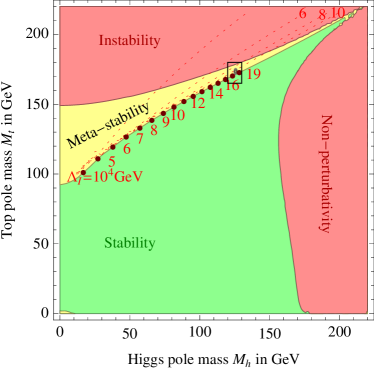
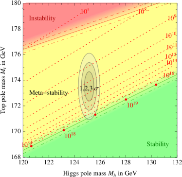
Figure 10: The standard model phase diagram in the $(M_{h},M_{t})$ plane. Images taken from Ref. [31].

Let us describe how the standard model phase diagram (which by definition assumes the standard model in isolation) is obtained and comment on possible interpretations of the fact that the experimental values of the standard model parameters seem to lie at the boundary between the stability and metastability region.

Instability/Metastability boundary

The probability of nucleating a bubble of true vacuum during the history of the Universe can be estimated as

$$p=\frac{\gamma}{{\mathcal{V}}_{3}}\left({\mathcal{V}_{3}}T\right)_{\rm light-cone},$$ (5.68)

with the space-time volume of our past light-cone given by [31]

$$\left({\mathcal{V}_{3}}T\right)_{\rm light-cone}\approx\frac{0.15}{H_{0}^{4}},$$ (5.69)

and $H_{0}=1.44\times 10^{-42}$ GeV being the present Hubble constant. The boundary region between instability (red) and metastability (yellow) in Fig. 10 is obtained by setting $p=1$ as a function of the top and Higgs pole masses.

Metastability/Stability boundary

The absolute stability condition was already discussed in Sect. 4.5 (cf. Eqs. (4.97)–(4.98) and Eqs. (4.100)–(4.100)) and reads

$$\lambda_{\rm eff}(\mu_{c})=\beta_{\lambda_{\rm eff}}(\mu_{c})=0,$$ (5.70)

where $\beta_{\lambda_{\rm eff}}=\mu\frac{d\lambda_{\rm eff}}{d\mu}$ and we have neglected small corrections of order $(v/\mu_{c})^{2}\approx 10^{-30}$ which corresponds to approximating $V_{\rm eff}(\phi)=\frac{1}{4}\lambda_{\rm eff}(\phi)\phi^{4}$. A more accurate stability criterium, which takes into account the consistent use of the $\hbar$ expansion of the standard model effective potential, was formulated in Ref. [36].

The critical line between metastability (yellow) and stability (green) in Fig. 10 is obtained by selecting the region in the $(M_{h},M_{t})$ plane where Eq. (5.70) holds. The technical tools entering the high-energy extrapolation of the standard model effective potential have been developed dramatically after the Higgs discovery and involve the calculation of beta functions [69, 29, 28, 70], threshold corrections at the $M_{t}$ mass scale [61, 62, 31, 71] and the fixed-order standard model effective potential [72, 73, 74]. With these ingredients at hand, one arrives to the remarkable conclusion that the electroweak vacuum is near-critical. While the central values of the standard model parameters point to the metastability region, with a lifetime way larger than the age of the Universe, absolute stability is excluded only between 2 and 3$\sigma$ confidence level (cf. right panel in Fig. 10). At the moment the leading uncertainty is of experimental nature and is due to the uncertainty on $M_{t}$ and $\alpha_{s}(M_{Z})$.

The main message of the standard model phase diagram is that the standard model can be consistently extrapolated up to the Planck scale. Pushing its interpretation even further, the apparent near-criticality of the standard model vacuum has triggered many speculations about the possible dynamics behind that (see e.g. [31, 75]).

5.6 Ultraviolet sensitivity and new physics

Physical degrees of freedom beyond those present in the standard model are expected, both on the basis of some experimental observations (massive neutrinos, dark matter, etc.) and of theoretical considerations (e.g. the naturalness problem). The presence of extra degrees of freedom can in general affect the standard model effective potential, possibly modifying, or even invalidating, the conclusions of the previous sections about the stability of the electroweak ground state. In such cases, the study of the electroweak vacuum lifetime is still a useful tool in order to constrain extensions of the standard model: non-standard physics should not make the electroweak vacuum too unstable.

The lifetime of the electroweak vacuum is obviously sensitive to new physics if its mass scale is $M<\overline{\mu}\approx 10^{17}$ GeV, since the standard model bounce gets directly affected. On the other hand, also new physics with $M\gg\overline{\mu}$ can enhance the tunnelling rate, e.g. by opening new decay channels for the electroweak vacuum [4, 76, 77, 78, 20, 79].

Such non-decoupling behaviour of ultraviolet physics might appear counter-intuitive. In quantum mechanics the shape of the potential beyond the barrier does not affect the tunnelling rate through the barrier itself. The case of quantum field theory is different. As shown in Sect. 3.4, the generalization of the potential barrier in quantum field theory involves a space-time integral of the scalar potential evaluated at the bounce configuration $\phi_{b}(r)$; as a consequence, all energy scales between 0 and $\phi_{b}(0)$ are relevant.

The impact of non-standard physics on the ground state lifetime can be assessed parametrizing new physics effects on the scalar potential by non-renormalizable operators. For example, in Ref. [4] it was proposed to modify the standard model scalar potential as

$$V(\phi)=\frac{1}{4}\lambda\phi^{4}+\frac{\lambda_{6}}{6M^{2}}\phi^{6}+\frac{\lambda_{8}}{8M^{4}}\phi^{8},$$ (5.71)

where $\lambda$ is the standard Higgs self-coupling, $\lambda_{6},\lambda_{8}$ are assumed to be of order one, and $M$ is the energy scale at which new physics effects become relevant. The potential in Eq. (5.71) is not meant to be a realistic ultraviolet completion of the standard model. From an effective field theory perspective, for instance, a more realistic picture would be obtained by considering a full tower of higher dimensional operators, including derivative operators as well. In the present discussion, we do not address the question of how specific models can affect the standard model vacuum lifetime, but just use the potential in Eq. (5.71) as a toy model in order to parametrize new physics effects.

The inclusion of two non-renormalizable terms in Eq. (5.71) does not allow us anymore to find an analytical solution of the bounce equation and one has to proceed numerically. The sensitivity of the tunnelling rate to new physics at very large energy scales can be assessed by comparing the potential energy barrier obtained with the potential in Eq. (5.71) with the one in the pure standard model. Following the definitions in Eqs. (3.45)–(3.47), for the standard model case with $\lambda<0$ one finds:

$$U_{\nabla}[\phi_{b}]=\phantom{-}\frac{2\pi^{2}}{\left|\lambda\right|R}\left(\frac{1}{1+\frac{\tau^{2}}{R^{2}}}\right)^{\frac{3}{2}},\qquad U_{V}[\phi_{b}]=-\frac{2\pi^{2}}{\left|\lambda\right|R}\left(\frac{1}{1+\frac{\tau^{2}}{R^{2}}}\right)^{\frac{5}{2}},$$ (5.72)

which have opposite sign, while their sum

$$U[\phi_{b}]=U_{\nabla}[\phi_{b}]+U_{V}[\phi_{b}]=\frac{2\pi^{2}}{\left|\lambda\right|R}\left(\frac{1}{1+\frac{\tau^{2}}{R^{2}}}\right)^{\frac{3}{2}}\frac{\frac{\tau^{2}}{R^{2}}}{1+\frac{\tau^{2}}{R^{2}}},$$ (5.73)

is positive, thus providing a true potential barrier.

The potential barrier in the presence of non-renormalizable terms in the scalar potential as in Eq. (5.71) can be computed by solving numerically the bounce equation. In Fig. 11 we compare the barrier $U[\phi_{b}]$ in the presence of new physics (orange) and in the pure standard model (blue). We have chosen $\lambda=\lambda(\overline{\mu})\simeq-0.01345$ (corresponding to the minimum of $\lambda(\mu)$ in the standard model), $\lambda_{6}=-2$ and $\lambda_{8}=2.1$, and we have set $M=M_{\rm Pl}$ for the scale of new physics. While the two barriers have comparable heights, the area under the curve which corresponds to the inclusion of new physics in this case is considerably smaller, which results in a much shorter lifetime of the metastable ground state for this particular choice of the parameters.

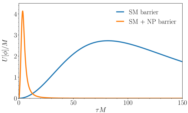
Figure 11: Potential barrier with and without the contribution of new physics. The values chosen for the new physics parameters are $\lambda_{6}=-2$, $\lambda_{8}=2.1$.

The above discussion can be generalized to the case of more non-renormalizable terms, including derivative operators, or even renormalizable ultraviolet completions of the standard model (see also [78, 80]). On the other hand, specific embeddings of the standard model into ultraviolet theories at the Planck scale can help in taming new instabilities of the Higgs potential [81].

Summarizing, while new physics at scales $M<\overline{\mu}\approx 10^{17}$ GeV can affect the decay rate of the standard model vacuum in any direction (possibly stabilizing the electroweak vacuum), modifications of the standard model potential at scales $M\gg\overline{\mu}\approx 10^{17}$ can only shorten the lifetime of the electroweak vacuum, whenever they lead to a new bounce solution which is related to a new, deeper minimum around the scale $M$.

6 Gravitational effects on vacuum decay

We have seen that very high energy scales are involved in the study of the metastability of the standard model ground state: the running coupling constant of the Higgs boson, $\lambda(\mu)$ becomes negative at $\mu\sim 10^{10}$ GeV, and reaches its maximum negative value (which determines the ground state lifetime) at $\mu=\overline{\mu}\approx 10^{17}$ GeV. It is therefore natural to ask whether gravitational effects become relevant in this regime. Indeed, the typical scale of gravitational interactions, the Planck mass $M_{\rm Pl}=1.22\times 10^{19}$ GeV, is only a couple of orders of magnitude larger than $\overline{\mu}$.

This issue was first addressed by Coleman and De Luccia in Ref. [5], where they considered the effects of gravity on the decay of a metastable vacuum in quantum field theory. In this section we will review their work, which allows us to introduce the relevant formalism. Next, following Ref. [6], we will apply the formalism of Coleman and De Luccia to the standard model. More recent developments on vacuum decay in the presence of gravity can be found e.g. in Refs. [82, 83].

6.1 The tunnelling rate in the presence of gravity

The inclusion of gravity in the calculation of the decay rate of the standard model vacuum is in principle straightforward: one must find a configuration $\phi_{b}(x)$ of the Higgs field which is a stationary point of the Euclidean Einstein-Hilbert action

$$S_{g}=\int d^{4}x\,\sqrt{g}\left[\frac{1}{2}\partial_{\mu}\phi_{b}\,\partial_{\nu}\phi_{b}\,g^{\mu\nu}+V(\phi_{b})-\frac{\mathcal{R}}{2\kappa}\right],$$ (6.1)

where $\mathcal{R}$ is the Riemann curvature, and

$$\kappa=8\pi G_{N}=\frac{8\pi}{M_{\rm Pl}^{2}},$$ (6.2)

where $G_{N}$ is the Newton constant and $M_{\rm Pl}=1.22\times 10^{19}$ GeV is the Planck mass. We will limit ourselves to the case of minimal coupling to gravity, which formally corresponds to the leading order in the $M_{\rm Pl}$ expansion. The impact on the tunnelling rate of unknown non-minimal coupling terms in the Einstein-Hilbert-Higgs action was addressed e.g. in Refs. [84, 85].

A difficulty immediately arises: contrary to the case of a flat spacetime, there is no guarantee that the bounce solution is $\,{\rm O}(4)$ invariant. We will make this assumption, which simplifies considerably the problem, but it should be kept in mind that a bounce solution with a smaller value of the action and no $\,{\rm O}(4)$ symmetry might in principle exist, although no example has been exhibited so far. We will therefore look for an $\,{\rm O}(4)$ invariant metric

$$ds^{2}=dr^{2}+\rho^{2}(r)d\Omega^{2}_{3},$$ (6.3)

where $d\Omega_{3}^{2}$ is the element of distance on a unit three-sphere,

$$d\Omega^{2}_{3}=d\chi^{2}+\sin^{2}\chi d\theta^{2}+\sin^{2}\theta d\phi^{2},$$ (6.4)

and an $\,{\rm O}(4)$ invariant bounce $\phi_{b}(r)$, which obeys the field equations

$$\phi_{b}^{\prime\prime}+\frac{3\rho^{\prime}}{\rho}\phi_{b}^{\prime}=V^{\prime}(\phi_{b}),$$ (6.5)

$${\rho^{\prime}}^{2}=1+\frac{1}{3}\kappa\rho^{2}\left(\frac{1}{2}{\phi_{b}^{\prime}}^{2}-V(\phi_{b})\right).$$ (6.6)

The boundary conditions for the field equations depend on the topology of the solution, which cannot be specified in advance. Since we are mainly interested in the problem of the stability of the standard model vacuum, we can neglect the small positive cosmological constant and assume a Minkowski-like background metric in the false vacuum. In such a case the bounce solution is non-compact, and $r\to\infty$. The boundary conditions leading to a finite bounce action are then

$$\phi_{b}^{\prime}(0)=0,\qquad\phi_{b}(\infty)=0,\qquad\rho(0)=0,\qquad\rho(\infty)=r,$$ (6.7)

where both the false vacuum and the value of the potential on the false vacuum are set to zero and the metric is asymptotically Minkowski-like. The condition $\rho(0)=0$ is less obvious and comes from the fact that $\rho(r)$ must have at least one zero which can be set to $r=0$ by translational invariance [7]. The Euclidean action Eq. (6.1) takes the form

$$S_{g}[\phi_{b},g]=2\pi^{2}\int_{0}^{\infty}dr\,\left[\rho^{3}\left(\frac{{\phi_{b}^{\prime}}^{2}}{2}+V(\phi_{b})\right)+\frac{3}{\kappa}\left(\rho^{2}\rho^{\prime\prime}+\rho{\rho^{\prime}}^{2}-\rho\right)\right].$$ (6.8)

The bounce action can be rewritten in a simpler form by a generalization of the virial theorem, proven in Sect. 3.1 in the flat-space case. Let us assume that the action is stationary upon variations of $\phi_{b}(x)$ and $g^{\mu\nu}(x)$; then in particular it should be stationary upon the transformations

$$\phi_{b}(x)\to\phi_{b}(bx),$$ (6.9)

$$g^{\mu\nu}(x)\to g^{\mu\nu}(bx),$$ (6.10)

which imply

$${\mathcal{R}}(x)\to b^{2}{\mathcal{R}}(bx).$$ (6.11)

We find

$$S_{g}\to S_{g}(b),$$ (6.12)

where

$$S_{g}(b) =\int d^{4}x\,\sqrt{g(bx)}\Bigg{[}\frac{1}{2}\frac{\partial\phi_{b}(bx)}{\partial x^{\mu}}\frac{\partial\phi_{b}(bx)}{\partial x^{\nu}}g^{\mu\nu}(bx)-\frac{b^{2}{\mathcal{R}}(bx)}{2\kappa}+V(\phi_{b}(bx))\Bigg{]}$$

$$=\int d^{4}x\,\sqrt{g(x)}\Bigg{[}\frac{1}{2b^{2}}\frac{\partial\phi_{b}(x)}{\partial x^{\mu}}\frac{\partial\phi_{b}(x)}{\partial x^{\nu}}g^{\mu\nu}(x)-\frac{{\mathcal{R}}(x)}{2b^{2}\kappa}+\frac{1}{b^{4}}V(\phi_{b}(x))\Bigg{]}.$$ (6.13)

The stationarity condition

$$\left.\frac{dS_{g}(b)}{db}\right|_{b=1}=0$$ (6.14)

gives a relationship between the derivative terms and the potential term in the action:

$$\int d^{4}x\,\sqrt{g(x)}\left[\frac{1}{2}\frac{\partial\phi_{b}(x)}{\partial x^{\mu}}\frac{\partial\phi_{b}(x)}{\partial x^{\nu}}g^{\mu\nu}(x)-\frac{{\mathcal{R}}(x)}{2\kappa}\right]=-2\int d^{4}x\,\sqrt{g(x)}V(\phi_{b}(x)).$$ (6.15)

Hence

$$S_{g}[\phi_{b},g]=-\int d^{4}x\,\sqrt{g(x)}V(\phi_{b}(x)).$$ (6.16)

In the flat-space limit this expression reproduces the standard virialized form of the action [2]. Assuming an $\,{\rm O}(4)$ invariant metric, Eq. (6.16) becomes (see also [85])

$$S_{g}[\phi_{b},g]=-2\pi^{2}\int_{0}^{\infty}dr\,\rho^{3}(r)V(\phi_{b}(r)).$$ (6.17)

Eq. (6.17) turns out to be much more useful than the equivalent form Eq. (6.8) in numerical estimates of the tunnelling rate, because the last two terms in Eq. (6.8) are both divergent for $r\to\infty$, while their difference is finite.

6.2 Perturbative solution of the field equations

The field equations (6.5, 6.6) cannot be solved analytically. Since the effects of gravity are typically small, it is tempting to look for a solution as an expansion in powers of $\kappa$, as suggested in Ref. [6], and to neglect systematically all terms of order $\kappa^{2}$ and higher. To this purpose, one must expand $\phi_{b}$ to order $\kappa$ and $\rho$ to order $\kappa^{2}$, because of the $\kappa^{-1}$ coefficient in the Einstein-Hilbert action:

$$\phi_{b}=\phi_{b0}+\kappa\phi_{b1}+O(\kappa^{2}),$$ (6.18)

$$\rho=\rho_{0}+\kappa\rho_{1}+\kappa^{2}\rho_{2}+O(\kappa^{3}),$$ (6.19)

where $\phi_{b0}$ is the bounce in the absence of gravity, and

$$\rho_{0}(r)=r,$$ (6.20)

as appropriate for a flat metric. The two equations for the order-$\kappa$ corrections:

$$\phi_{b1}^{\prime\prime}+\frac{3}{r}\phi_{b1}^{\prime}+\frac{3}{r}\left(\rho_{1}^{\prime}-\frac{\rho_{1}}{r}\right)\phi_{b0}^{\prime}=V^{\prime\prime}(\phi_{b0})\phi_{b1}$$ (6.21)

$$\rho_{1}^{\prime}=\frac{1}{12}r^{2}\left({\phi_{b0}^{\prime}}^{2}-2V(\phi_{b0})\right)$$ (6.22)

are no longer coupled to each other.

It is interesting to note that, to order $\kappa$, the correction terms $\phi_{b1}$ and $\rho_{2}$ do not affect the Euclidean action. Indeed, the first term in Eq. (6.8) becomes

$$\rho^{3}\left(\frac{{\phi_{b}^{\prime}}^{2}}{2}+V(\phi_{b})\right)=r^{3}\left(\frac{{\phi_{b0}^{\prime}}^{2}}{2}+V(\phi_{b0})\right)$$

$$\qquad+\kappa\left[3r^{2}\rho_{1}\left(\frac{{\phi_{b0}^{\prime}}^{2}}{2}+V(\phi_{b0})\right)+r^{3}\left(\phi_{b1}^{\prime}\phi_{b0}^{\prime}+\phi_{b1}V^{\prime}(\phi_{b0})\right)\right]+O(\kappa^{2}).$$ (6.23)

We now observe that

$$r^{3}\left(\phi_{b1}^{\prime}\phi_{b0}^{\prime}+\phi_{b1}V^{\prime}(\phi_{b0})\right)=\frac{d}{dr}\left(r^{3}\phi_{b1}\phi_{b0}^{\prime}\right),$$ (6.24)

where we have used the flat-space field equation for $\phi_{b0}$

$$\phi_{b0}^{\prime\prime}+\frac{3}{r}\phi_{b0}^{\prime}=V^{\prime}(\phi_{b0})$$ (6.25)

to eliminate $V^{\prime}(\phi_{b0})$. Hence, the last term in Eq. (6.23) gives no contribution to the action, provided

$$\lim_{r\to 0}\left(r^{3}\phi_{b1}\phi_{b0}^{\prime}\right)=\lim_{r\to+\infty}\left(r^{3}\phi_{b1}\phi_{b0}^{\prime}\right)=0.$$ (6.26)

Furthermore, expanding $\rho$ to order $\kappa^{2}$ we find

$$\rho^{2}\rho^{\prime\prime}+\rho{\rho^{\prime}}^{2}-\rho=\kappa\frac{d}{dr}\left(r^{2}\rho_{1}^{\prime}\right)+\kappa^{2}\frac{d}{dr}\left(r^{2}\rho_{2}^{\prime}\right)+\kappa^{2}\left(2\rho_{1}\rho_{1}^{\prime}+2r\rho_{1}\rho_{1}^{\prime\prime}+r{\rho_{1}^{\prime}}^{2}\right).$$ (6.27)

The only $\rho_{2}$-dependent term vanishes upon integration. Therefore, the bounce action depends only on $\phi_{b0},\rho_{0},\rho_{1}$, up to corrections of order $\kappa^{2}$:

$$S_{g}[\phi_{b},g] =2\pi^{2}\int_{0}^{\infty}dr\,\Bigg{[}r^{3}\left(\frac{{\phi_{b0}^{\prime}}^{2}}{2}+V(\phi_{b0})\right)+3\kappa r^{2}\rho_{1}\left(\frac{{\phi_{b0}^{\prime}}^{2}}{2}+V(\phi_{b0})\right)$$

$$+3\kappa\left(2\rho_{1}\rho_{1}^{\prime}+2r\rho_{1}\rho_{1}^{\prime\prime}+r{\rho_{1}^{\prime}}^{2}\right)\Bigg{]}+O(\kappa^{2}).$$ (6.28)

6.3 Decay of the standard model vacuum in the presence of gravity

The formalism outlined in the previous sections can be applied to the standard model [6]. As in the case of a flat space-time, we approximate the standard model scalar potential by

$$V(\phi)=\frac{1}{4}\lambda\phi^{4},$$ (6.29)

with $\lambda=\lambda(\overline{\mu})<0$. The linearized field equations, Eqs. (6.21)–(6.22), take the form

$$\phi_{b1}^{\prime\prime}+\frac{3}{r}\phi_{b1}^{\prime}+\frac{3}{r}\left(\rho_{1}^{\prime}-\frac{\rho_{1}}{r}\right)\phi_{b0}^{\prime}=3\lambda\phi_{b0}^{2}\phi_{b1}$$ (6.30)

$$\rho_{1}^{\prime}=\frac{1}{12}r^{2}\left({\phi_{b0}^{\prime}}^{2}-\frac{\lambda}{2}\phi_{b0}^{4}\right),$$ (6.31)

where $\phi_{b0}$ is the bounce in the absence of gravity, the Fubini-Lipatov bounce Eq. (5.12) or (5.13). We have shown in the previous section that the first order correction to the bounce, $\phi_{b1}(r)$, does not affect the value of the bounce action. On the other hand, Eq. (6.22) is immediately integrated, to give

$$\rho_{1}(r)=\frac{1}{3|\lambda|R}\frac{(1+x^{2})^{2}\arctan x+x(x^{2}-1)}{(1+x^{2})^{2}};\qquad x=\frac{r}{R}.$$ (6.32)

This is sufficient to make an estimate of the impact of gravitational interactions on the decay rate of the standard model vacuum, to first order in $\kappa$. One finds that the value of the effective bounce action is shifted by

$$\Delta\Gamma[\phi_{b}]=\frac{256\pi^{3}}{45(RM_{\rm Pl}\lambda)^{2}}.$$ (6.33)

There is however a difficulty that arises in the computation of higher-order corrections, as pointed out in Ref. [86], which is again related to the transformation properties of the action upon scale transformations. Adopting the approximate form of the scalar potential Eq. (6.29) a scale transformation

$$\phi_{b}(x)\to a\phi_{b}(ax),$$ (6.34)

$$g^{\mu\nu}(x)\to g^{\mu\nu}(ax),$$ (6.35)

$${\mathcal{R}}(x)\to a^{2}{\mathcal{R}}(ax)$$ (6.36)

transforms the action as

$$S_{g}\to S_{g}(a),$$ (6.37)

where

$$S_{g}(a) =\int d^{4}x\,\sqrt{g(ax)}\left[\frac{a^{2}}{2}\frac{\partial\phi_{b}(ax)}{\partial x^{\mu}}\frac{\partial\phi_{b}(ax)}{\partial x^{\nu}}g^{\mu\nu}(ax)+\frac{a^{4}\lambda}{4}\phi_{b}^{4}(ax)-\frac{a^{2}{\mathcal{R}}(ax)}{2\kappa}\right]$$

$$=\int d^{4}x\,\sqrt{g(x)}\left[\frac{1}{2}\frac{\partial\phi_{b}(x)}{\partial x^{\mu}}\frac{\partial\phi_{b}(x)}{\partial x^{\nu}}g^{\mu\nu}(x)+\frac{\lambda}{4}\phi_{b}^{4}(x)-\frac{{\mathcal{R}}(x)}{2a^{2}\kappa}\right].$$ (6.38)

The stationarity condition

$$a\left.\frac{dS_{g}(a)}{da}\right|_{a=1}=\int d^{4}x\,\sqrt{g(x)}\frac{{\mathcal{R}}(x)}{\kappa}=0$$ (6.39)

can only be satisfied in the flat limit $\mathcal{R}(y)=0$, or equivalently $\rho(r)=r$. But in this case Eq. (6.6) gives

$$\frac{1}{2}{\phi_{b}^{\prime}}^{2}-V(\phi_{b})=\frac{1}{2}{\phi_{b}^{\prime}}^{2}+\frac{|\lambda|}{4}\phi_{b}^{4}=0,$$ (6.40)

which is only possible if $\phi_{b}(r)=0$, similarly to what happens in the flat-space-time case with the introduction of a mass term in the scalar potential Eq. (6.29): the breaking of scale invariance leads to the disappearance of the bounce. This is confirmed by an explicit calculation of the order-$\kappa$ correction to the bounce. Eq. (6.30) can be solved analytically [84], with the following result:

$$\phi_{b1}(r) =\frac{1}{3R^{3}|\lambda|^{3/2}}\frac{4\sqrt{2}}{(1+x^{2})^{2}}\Bigg{[}c_{1}(x^{2}-1)+c_{2}\frac{1-17x^{2}-x^{2}(1-x^{2})(x^{2}+12\log x)}{2x^{2}}$$

$$+\frac{1}{15x^{2}}\frac{1+x^{2}(7-9x^{2})}{1+x^{2}}-x\arctan x+\frac{2}{5}(1-x^{2})\log\frac{1+x^{2}}{x^{2}}\Bigg{]},$$ (6.41)

where $c_{1}$ and $c_{2}$ are arbitrary constants. Since $\phi_{b0}(r)$ obeys the required asymptotic conditions for $\phi_{b}(r)$, namely $\phi_{b}^{\prime}(0)=\phi_{b}(\infty)=0$, the same conditions must also apply to $\phi_{b1}(r)$. We find

$$\lim_{r\to\infty}\phi_{b1}(r)=\frac{2\sqrt{2}}{3R^{3}|\lambda|^{3/2}}c_{2}$$ (6.42)

and

$$\phi_{b1}(r)\sim\frac{1}{R^{3}|\lambda|^{3/2}}\frac{4\sqrt{2}}{3}\left(\frac{c_{2}}{2}+\frac{1}{15}\right)\left(\frac{1}{x^{2}}-12\log x\right)+\text{regular terms}$$ (6.43)

for $r$ close to zero. Hence, the two boundary conditions cannot be satisfied simultaneously.

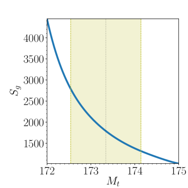
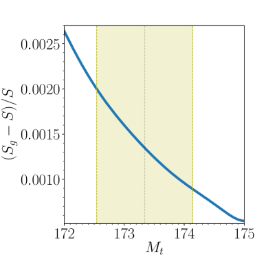
Figure 12: Left panel: value of the action as a function of the top quark mass, including gravitational effects. Right panel: fractional difference between the action including or neglecting gravity. Displayed are also the central value of the top mass and its $1$-$\sigma$ uncertainty, $M_{t}=173.34\pm 0.8$.

On the other hand, when the scale dependence of the renormalized coupling is taken into account, the stationarity condition upon scale transformations becomes

$$a\left.\frac{dS_{g}(a)}{da}\right|_{a=1}=\int d^{4}x\,\sqrt{g(x)}\left[\frac{{\mathcal{R}}(x)}{\kappa}+\frac{1}{4}\beta(\lambda(\phi_{b}))\phi_{b}^{4}\right]=0,$$ (6.44)

and a non-vanishing bounce solution of the field equation can be found. We have checked that this is indeed the case by a numerical calculation (numerical methods to find the bounce in the presence of gravity are also reviewed in App. A.6). Comparing the action computed taking gravity into account, $S_{g}$, with the action computed in a flat space-time, $S$, we notice that gravity stabilizes the ground state, thus making its lifetime slightly longer.

Since one of the most important parameters describing the running of the coupling constant $\lambda$ is the mass of the top quark $M_{t}$, it is interesting to study how the lifetime of the ground state is modified by varying $M_{t}$ within its experimental uncertainty. In the left panel of Fig. 12 we represent the value of the action in the presence of gravity as a function of the top quark mass. As in the flat space-time case, a lower value for the top quark stabilizes the potential, making the ground state lifetime longer.

Furthermore, from the fractional difference between the action including or neglecting gravity in the right panel of Fig. 12 one can see that (especially for lower values of the top quark mass) the bounce action becomes larger in the presence of gravity and hence the vacuum lifetime is longer. The reason of this phenomenon can be better understood by thinking at the running of $\lambda$. A lower mass for the top quark means a larger energy scale involved in the tunnelling process since the zero of $\beta_{\lambda}$ is shifted at higher values, and hence gravitational effects are more important.

Finally, we remark that in the presence of new Planck-scale suppressed effective operators (cf. Sect. 5.6) the tunnelling rate might still be strongly enhanced, even after taking into account gravitational effects [87].

7 Conclusions

In this work, we have reviewed the phenomenon of quantum tunnelling both in ordinary quantum mechanics and quantum field theory. In particular, we have applied the formalism to the relevant case of the stability of the electroweak ground state in the standard model, which presents several subtle aspects related to the radiative instability of the Higgs potential and the approximate scale invariance of the electroweak theory at high-energy scales.

The present situation regarding the phase diagram of the standard model vacuum is represented in Fig. 10 (from Ref. [31]). Given the present value of the top quark mass, the standard model vacuum is metastable (with a lifetime much larger than the age of the Universe), although remarkably close to the absolute stability boundary which can be reached at the 2-3$\sigma$ level, depending on the uncertainty on the top quark mass. Future improvements on the measurement of the top quark mass, which may be decisively achieved with a dedicated top-threshold lepton collider [88], will be crucial in order to establish whether the electroweak ground state is metastable or absolutely stable.

The fate of the standard model vacuum is also deeply intertwined with the cosmological evolution of the Universe, a fascinating subject that we have completely omitted in this introductory review. For instance, the electroweak vacuum instability might have played an important role for the evolution of the Higgs field during inflation (see e.g. [89]). Moreover, finite temperature effects might enhance the decay rate due to thermal fluctuations which should be taken into account for the vacuum stability analysis in the early Universe (see e.g. [90]).

Although the vacuum decay rate in quantum field theory is inherently ultraviolet sensitive (new physics in the deep ultraviolet can always enhance the decay rate), the apparent near-criticality of the standard model vacuum (under the conservative hypothesis of no new physics between the electroweak and the Planck scale) hints to a deeper structure, that is possibly related to the hidden meaning of the standard model itself.

Appendix A Appendices

A.1 The semi-classical approximation in quantum mechanics

We consider a particle of mass $m$ moving in one space dimension: $x$ is the space coordinate, $p$ its conjugate momentum, and $U(x)$ the potential energy. The Hamiltonian is

$$H(p,x)=\frac{p^{2}}{2m}+U(x).$$ (A.1)

In classical physics, the particle’s motion is only allowed in the region defined by $E\geq U(x)$, where $E$ is the total particle energy. The values of $x$ for which $U(x)=E$ are usually called turning points, for obvious reasons.

In ordinary quantum mechanics one looks for stationary states $\psi(x)$, solutions of the time-independent Schrödinger equation

$$-\frac{\hbar^{2}}{2m}\psi^{\prime\prime}(x)+U(x)\psi(x)=E\psi(x)$$ (A.2)

(primes denote differentiation with respect to the argument.) Apart from a few simple cases, the stationary state wave functions can be only be determined in the context of some approximation framework. In the case of barrier penetration, the so-called semi-classical approximation proves especially useful [8, 9, 91].

The classical limit of quantum mechanics, $\hbar\to 0$, is a singular limit of Eq. (A.2): for $\hbar=0$ the derivative term disappears, and the equation has a different space of solutions. The correct way to take the classical limit is the following: the wave function is written

$$\psi(x)=\exp\left[i\frac{\sigma(x)}{\hbar}\right],$$ (A.3)

where $\sigma(x)$ is a complex function. In this way, all terms in Eq. (A.2) are of the same order as $\hbar\to 0$, because

$$\psi^{\prime\prime}(x)=-\frac{1}{\hbar^{2}}\left[{\sigma^{\prime}}^{2}(x)-i\hbar\sigma^{\prime\prime}(x)\right]\psi(x).$$ (A.4)

Eq. (A.2) takes the form

$${\sigma^{\prime}}^{2}(x)-i\hbar\sigma^{\prime\prime}(x)=2m\left[E-U(x)\right].$$ (A.5)

The complex function $\sigma(x)$ is assumed to have a power expansion in $\hbar$:

$$\sigma(x)=\sigma_{0}(x)+\frac{\hbar}{i}\sigma_{1}(x)+\left(\frac{\hbar}{i}\right)^{2}\sigma_{2}(x)+O(\hbar^{3}).$$ (A.6)

Replacing Eq. (A.6) in Eq. (A.5) we obtain a tower of differential equations for the coefficients $\sigma_{n}(x)$. To lowest order we get

$${\sigma_{0}^{\prime}}^{2}(x)=2m\left[E-U(x)\right],$$ (A.7)

which is immediately integrated:

$$\sigma_{0}(x)=\pm\int dx\,p(x),$$ (A.8)

where

$$p(x)=+\sqrt{2m\left[E-U(x)\right]}$$ (A.9)

is the classical particle momentum. Note that the term proportional to $\hbar$ in the l.h.s. of Eq. (A.5) can be neglected provided

$$|{\sigma^{\prime}}^{2}(x)|\gg\hbar|\sigma^{\prime\prime}(x)|,$$ (A.10)

or

$$\left|\hbar\frac{d}{dx}\frac{1}{\sigma^{\prime}(x)}\right|\simeq\left|\frac{d}{dx}\frac{\hbar}{p(x)}\right|\ll 1,$$ (A.11)

which means that the approximation is only valid where the particle wavelength $\lambda=\frac{h}{p}$ does not vary too much over distances of its same order. This is clearly not the case in the vicinity of turning points, where $p(x)=0$ and $\lambda\to\infty$.

Including one more term in the $\hbar$ expansion we get

$$2\sigma_{1}^{\prime}(x)\sigma_{0}^{\prime}(x)+\sigma_{0}^{\prime\prime}(x)=0,$$ (A.12)

which gives

$$\sigma_{1}^{\prime}(x)=-\frac{1}{2}\frac{\sigma_{0}^{\prime\prime}(x)}{\sigma_{0}^{\prime}(x)}=-\frac{p^{\prime}(x)}{2p(x)};\qquad\sigma_{1}(x)=\log\frac{1}{\sqrt{|p(x)|}}$$ (A.13)

up to an arbitrary integration constant. Hence, the wave function in the semi-classical approximation, including corrections up to order $\hbar$ in $\sigma(x)$, is given by

$$\psi(x)=\frac{C_{1}}{\sqrt{p(x)}}e^{\frac{i}{\hbar}\int_{a}^{x}p(x^{\prime})dx^{\prime}}+\frac{C_{2}}{\sqrt{p(x)}}e^{-\frac{i}{\hbar}\int_{a}^{x}p(x^{\prime})dx^{\prime}}$$ (A.14)

in the classically allowed regions, where $p(x)$ is real and positive, and

$$\psi(x)=\frac{D_{1}}{\sqrt{|p(x)|}}e^{-\frac{1}{\hbar}\int_{a}^{x}|p(x^{\prime})|dx^{\prime}}+\frac{D_{2}}{\sqrt{|p(x)|}}e^{\frac{1}{\hbar}\int_{a}^{x}|p(x^{\prime})|dx^{\prime}}$$ (A.15)

in the classically forbidden ones, where $p(x)$ is purely imaginary. In the latter case, when $x\to\pm\infty$ only one of the two terms must be retained, to ensure normalizability of the wave function. Otherwise, one of the two terms is exponentially suppressed with respect to the other, and must be consistently neglected. In Eqs. (A.14, A.15), $a$ is an arbitrary reference point on the $x$ axis. A different choice of $a$ can be absorbed in a redefinition of the constants $C_{i},D_{i}$. Higher-order terms in the expansion of $\sigma(x)$ in powers of $\hbar$ are very rarely needed.

The constants $C_{1},C_{2},D_{1},D_{2}$ must be fixed on the basis of normalization and continuity of the wave function and its first derivative at turning points. This is not a trivial task, because the semi-classical approximation does not hold in the vicinity of a turning point. A way to circumvent this difficulty is the following. To be definite, let us assume that $x=a$ is a turning point, with $E<U(x)$ for $x>a$. Then

$$\psi(x)=\left\{\begin{array}[]{ll}\frac{C_{1}}{\sqrt{p(x)}}e^{\frac{i}{\hbar}\int_{a}^{x}p(x^{\prime})dx^{\prime}}+\frac{C_{2}}{\sqrt{p(x)}}e^{-\frac{i}{\hbar}\int_{a}^{x}p(x^{\prime})dx^{\prime}}&x\ll a\\ \frac{D}{\sqrt{|p(x)|}}e^{-\frac{1}{\hbar}\int_{a}^{x}|p(x^{\prime})|dx^{\prime}}&x\gg a\end{array}\right..$$ (A.16)

Our task is relating $D$ to $C_{1}$ and $C_{2}$ by requiring the continuity of the wave function and its first derivative at $x=a$. These conditions cannot be imposed directly on $\psi(x)$ as given in Eq. (A.16), because the semi-classical approximation fails in the vicinity of a turning point. We will instead continue analytically $\psi(x)$ in the complex plane $x$ from the real axis to the right of the turning point, ${\rm Re\,}x>a$, to the real axis to the left ${\rm Re\,}x<a$, following a path which is never too close to the turning point. For example, we may choose a half-circle with center $a$ and radius $r$, in the upper or in the lower complex half-plane, provided $r$ is large enough for the semi-classical approximation to hold. We further assume that we can choose $r$ so that the potential energy $U(x)$ can be reliably expanded in Taylor series to first order in $x-a$ for all complex $x$ with $|x-a|=r$:

$$U(x)=U(a)+U^{\prime}(a)(x-a)+O(r^{2})=E-F(x-a)+O(r^{2}),$$ (A.17)

with $F=-U^{\prime}(a)<0$ by assumption. Neglecting terms of order $r^{2}$ and higher in $U(x)$ the exponent of $\psi(x)$ for $x>a$ reads

$$\frac{i}{\hbar}\sigma_{0}(x)=-\frac{1}{\hbar}\int_{a}^{x}|p(x^{\prime})|dx^{\prime}=-\frac{2}{3\hbar}\sqrt{2m|F|}(x-a)^{\frac{3}{2}}.$$ (A.18)

We now set

$$x=a+re^{i\theta}$$ (A.19)

and continue analytically the wave function following the half-circle in the upper complex plane. We get

$$\frac{i}{\hbar}\sigma_{0}(x)=-\frac{2}{3\hbar}\sqrt{2m|F|}r^{\frac{3}{2}}e^{\frac{3}{2}i\theta};\qquad 0\leq\theta\leq\pi.$$ (A.20)

For $\theta=\pi$

$$\frac{i}{\hbar}\sigma_{0}(x)=\frac{2i}{3\hbar}\sqrt{2m|F|}r^{\frac{3}{2}}=-\frac{i}{\hbar}\int_{a}^{x}p(x^{\prime})dx^{\prime},$$ (A.21)

which is the exponent of the term proportional to $C_{2}$ in Eq. (A.16). On the other hand,

$$\frac{1}{\sqrt{|p(x)|}}=\frac{1}{(2m|F|)^{\frac{1}{4}}}(x-a)^{-\frac{1}{4}}$$ (A.22)

which, by the same argument, is continued to

$$\frac{1}{(2m|F|)^{\frac{1}{4}}}r^{-\frac{1}{4}}e^{-\frac{1}{4}i\pi}=\frac{1}{\sqrt{p(x)}}e^{-\frac{1}{4}i\pi}.$$ (A.23)

We therefore conclude that

$$C_{2}=De^{-\frac{1}{4}i\pi}.$$ (A.24)

Following the half-circle in the lower half-plane we obtain, by an analogous argument,

$$C_{1}=De^{\frac{1}{4}i\pi}.$$ (A.25)

Finally,

$$\psi(x)=\left\{\begin{array}[]{ll}\frac{2D}{\sqrt{p(x)}}\cos\left[\frac{1}{\hbar}\int_{a}^{x}p(x^{\prime})dx^{\prime}+\frac{\pi}{4}\right]&x\ll a\\ \frac{D}{\sqrt{|p(x)|}}e^{-\frac{1}{\hbar}\int_{a}^{x}|p(x^{\prime})|dx^{\prime}}&x\gg a\end{array}\right..$$ (A.26)

This formula was obtained in the case when the region $x>a$ is classically forbidden; it is easy to show that in the general case

$$\psi(x)=\left\{\begin{array}[]{ll}\frac{2D}{\sqrt{p(x)}}\cos\left[\frac{1}{\hbar}\left|\int_{a}^{x}p(x^{\prime})dx^{\prime}\right|-\frac{\pi}{4}\right]&U(x)<E\\ \frac{D}{\sqrt{|p(x)|}}e^{-\frac{1}{\hbar}\left|\int_{a}^{x}p(x^{\prime})dx^{\prime}\right|}&U(x)>E\end{array}\right..$$ (A.27)

A.2 Double-well potential in the semi-classical approximation

In Sect. 2.2 we have discussed how the double-well potential can be studied in the path integral formalism. In this Appendix, we review the standard formulation of the same problem in the semi-classical approximation. We will follow the discussion presented in Ref. [8].

We consider again the hamiltonian of a particle moving in one dimension under the effect of a potential with two degenerate minima:

$$H=\frac{1}{2}m\left(\frac{dx}{dt}\right)^{2}+U(x),$$ (A.28)

where $U(x)$ is an even function, with two minima at $x=\pm a$ and a local maximum at $x=0$. We further assume $U(\pm a)=0$, and define $U^{\prime\prime}(\pm a)=m\omega^{2}$. An example of a potential energy with these features is

$$U(x)=\frac{m\omega^{2}}{8a^{2}}(x^{2}-a^{2})^{2},$$ (A.29)

but the discussion can be kept at a general level, and reference to a specific form of the potential is not needed.

If the potential energy barrier separating the two minima were infinitely high and broad, there would be two identical towers of energy eigenvalues and eigenstates, corresponding to the two potential wells at $x=\pm a$. The wave functions $\psi(\pm x)$ of the fundamental states, with energy $E_{0}$, are strongly peaked around $x=\pm a$, and decrease exponentially away from the potential minima. The function $\psi(x)$ is a solution of

$$-\frac{\hbar^{2}}{2m}\psi^{\prime\prime}(x)+U(x)\psi(x)=E_{0}\psi(x).$$ (A.30)

We now take quantum tunnelling into account, under the assumption that the semi-classical approximation is reliable. Because the potential is parity-even, the wave functions of the two lowest-energy states are

$$\psi_{1}(x)=\frac{1}{\sqrt{2}}\left[\psi(x)+\psi(-x)\right]$$ (A.31)

$$\psi_{2}(x)=\frac{1}{\sqrt{2}}\left[\psi(x)-\psi(-x)\right]$$ (A.32)

with energies $E_{1}$ and $E_{2}$ respectively:

$$-\frac{\hbar^{2}}{2m}\psi_{1}^{\prime\prime}(x)+U(x)\psi_{1}(x)=E_{1}\psi_{1}(x)$$ (A.33)

$$-\frac{\hbar^{2}}{2m}\psi_{2}^{\prime\prime}(x)+U(x)\psi_{2}(x)=E_{2}\psi_{2}(x),$$ (A.34)

and $E_{1}<E_{2}$ because $\psi_{2}(x)$ has a node in $x=0$. Furthermore, the two wave functions are approximately normalized, because $\psi(x)$ has almost no overlap with $\psi(-x)$. Eqs. (A.30, A.33, A.34) can be combined and integrated, to obtain

$$-\frac{\hbar^{2}}{2m}\int_{0}^{+\infty}dx\,\left[\psi_{1}(x)\psi^{\prime\prime}(x)-\psi_{1}^{\prime\prime}(x)\psi(x)\right] =(E_{0}-E_{1})\int_{0}^{+\infty}dx\,\psi(x)\psi_{1}(x)$$ (A.35)

$$-\frac{\hbar^{2}}{2m}\int_{0}^{+\infty}dx\,\left[\psi_{2}(x)\psi^{\prime\prime}(x)-\psi_{2}^{\prime\prime}(x)\psi(x)\right] =(E_{0}-E_{2})\int_{0}^{+\infty}dx\,\psi(x)\psi_{2}(x).$$ (A.36)

The integrals are readily performed by means of Eqs. (A.31, A.32), which give $\psi^{\prime}_{1}(0)=\psi_{2}(0)=0$. We obtain

$$E_{1} =E_{0}-\frac{\hbar^{2}}{m}\psi(0)\psi^{\prime}(0)$$ (A.37)

$$E_{2} =E_{0}+\frac{\hbar^{2}}{m}\psi^{\prime}(0)\psi(0)$$ (A.38)

and therefore

$$E_{2}-E_{1}=\frac{2\hbar^{2}}{m}\psi(0)\psi^{\prime}(0).$$ (A.39)

It is at this point that the semi-classical approximation comes into play. The value of the wave function at the origin can be computed using the approximate expression Eq. (A.27) for the wave function; we find

$$\psi(0)=\frac{D}{\sqrt{|p(0)|}}e^{-\frac{1}{\hbar}\int_{0}^{x_{-}}dx\,|p(x)|},\qquad\psi^{\prime}(0)=\frac{D\sqrt{|p(0)|}}{\hbar}e^{-\frac{1}{\hbar}\int_{0}^{x_{-}}dx\,|p(x)|}$$ (A.40)

where $x_{\pm}$ are the classical turning points corresponding to the energy $E_{0}$ for the potential well at $x=a$:

$$U(x_{\pm})=E_{0};\qquad x_{\pm}>0.$$ (A.41)

Therefore

$$E_{2}-E_{1}=\frac{2\hbar}{m}D^{2}e^{-\frac{1}{\hbar}\int_{-x_{-}}^{x_{-}}dx\,|p(x)|}$$ (A.42)

where we have used $U(x)=U(-x)$.

The constant $D$ can be obtained from the normalization condition of the wave function. Neglecting the exponentially suppressed contributions from the classically forbidden regions, we get

$$\int_{-\infty}^{+\infty}|\psi(x)|^{2}dx=4D^{2}\int_{x_{-}}^{x_{+}}dx\,\frac{1}{p(x)}\cos^{2}\left[\frac{1}{\hbar}\left|\int_{x_{-}}^{x}p(x^{\prime})dx^{\prime}\right|-\frac{\pi}{4}\right]=1.$$ (A.43)

We may replace the cosine squared in the integrand by its average over a period of the classical motion, $1/2$, to obtain

$$2D^{2}\int_{x_{-}}^{x_{+}}\frac{dx}{p(x)}=1.$$ (A.44)

Furthermore,

$$\int_{x_{-}}^{x_{+}}\frac{dx}{p(x)}=\int_{t_{1}}^{t_{2}}\frac{dx}{dt}\frac{dt}{p(x)}=\frac{1}{m}(t_{2}-t_{1})=\frac{\pi}{m\omega},$$ (A.45)

which gives

$$D^{2}=\frac{m\omega}{2\pi}$$ (A.46)

and

$$E_{2}-E_{1}=\frac{\hbar\omega}{\pi}e^{-\frac{1}{\hbar}\int_{-x_{-}}^{x_{-}}dx\,|p(x)|};\qquad|p(x)|=\sqrt{2m(U(x)-E_{0})};\qquad U(x_{-})=E_{0}.$$ (A.47)

This is how the result is usually presented in textbooks (see e.g. [8]).

Since

$$U(x)=\frac{1}{2}m\omega^{2}(x-a)^{2}+O((x-a)^{3})$$ (A.48)

in the vicinity of $x=a$, we have

$$E_{0}\simeq\frac{\hbar\omega}{2};\qquad x_{\pm}\simeq a\pm\sqrt{\frac{\hbar}{m\omega}},$$ (A.49)

and the exponent of Eq. (A.47) reads

$$F(\hbar)=-\frac{2}{\hbar}\int_{0}^{a-\sqrt{\frac{\hbar}{m\omega}}}dx\,\sqrt{2mU(x)-\hbar m\omega}$$ (A.50)

The exponent $F(\hbar)$ is singular as $\log\hbar$ as $\hbar\to 0$, as can be seen by observing that, for small $\hbar$, the integration variable $x$ is close to $a$ at the upper integration bound, and $U(x)\sim\frac{1}{2}m\omega^{2}(a-x)^{2}$ in this region. In order take this singularity into account, we split the integration range in Eq. (A.50):

$$F(\hbar)=-\frac{2}{\hbar}\int_{0}^{a-\epsilon}dx\,\sqrt{2mU(x)-\hbar m\omega}-\frac{2}{\hbar}\int_{a-\epsilon}^{a-\sqrt{\frac{\hbar}{m\omega}}}dx\,\sqrt{2mU(x)-\hbar m\omega},$$ (A.51)

where $\epsilon$ is an arbitrary constant in the range $\sqrt{\frac{\hbar}{m\omega}}<\epsilon<a$. The integration range in the first integral now does not contain the singular point, and we may expand the integrand in powers of $\hbar$ to first order, while in the second integral we may approximate $U(x)$ as in Eq. (A.48) if $\epsilon$ is not too large. We get

$$F(\hbar)= -\frac{2}{\hbar}\int_{0}^{a-\epsilon}dx\,\sqrt{2mU(x)}+m\omega\int_{0}^{a-\epsilon}\frac{dx}{\sqrt{2mU(x)}}$$

$$-\frac{2m\omega}{\hbar}\int_{a-\epsilon}^{a-\sqrt{\frac{\hbar}{m\omega}}}dx\,\sqrt{(a-x)^{2}-\frac{\hbar}{m\omega}}+O(\hbar).$$ (A.52)

The last integral can be computed analytically. Neglecting $O(\hbar)$ corrections, and using Eq. (A.48) again whenever allowed, we get

$$F(\hbar)= -\frac{2}{\hbar}\int_{0}^{a}dx\,\sqrt{2mU(x)}-\frac{2m\omega}{\hbar}\int_{a}^{a-\epsilon}dx\,(a-x)$$

$$+\int_{0}^{a-\epsilon}dx\,\left[\frac{m\omega}{\sqrt{2mU(x)}}-\frac{1}{a-x}\right]+\int_{0}^{a-\epsilon}dx\,\frac{1}{a-x}$$

$$-\log\left[\sqrt{\frac{m\omega}{\hbar}}\left(\epsilon-\sqrt{\epsilon^{2}-\frac{\hbar}{m\omega}}\right)\right]-\frac{m\omega}{\hbar}\epsilon\sqrt{\epsilon^{2}-\frac{\hbar}{m\omega}}$$

$$= -\frac{2}{\hbar}\int_{0}^{a}dx\,\sqrt{2mU(x)}+\int_{0}^{a-\epsilon}dx\,\left[\frac{m\omega}{\sqrt{2mU(x)}}-\frac{1}{a-x}\right]$$

$$-\log\left[\frac{\epsilon^{2}}{a}\sqrt{\frac{m\omega}{\hbar}}\left(1-\sqrt{1-\frac{\hbar}{m\omega\epsilon^{2}}}\right)\right]+\frac{m\omega\epsilon^{2}}{\hbar}\left(1-\sqrt{1-\frac{\hbar}{m\omega\epsilon^{2}}}\right).$$ (A.53)

In the semi-classical limit $\hbar\ll\epsilon^{2}m\omega$ we have

$$1-\sqrt{1-\frac{\hbar}{m\omega\epsilon^{2}}}=\frac{\hbar}{2m\omega\epsilon^{2}}+O(\hbar^{2}),$$ (A.54)

so that

$$F(\hbar)=-\frac{2}{\hbar}\int_{0}^{a}dx\,\sqrt{2mU(x)}+\int_{0}^{a-\epsilon}dx\,\left[\frac{m\omega}{\sqrt{2mU(x)}}-\frac{1}{a-x}\right]+\log\left[2a\sqrt{\frac{m\omega}{\hbar}}\right]+\frac{1}{2}.$$ (A.55)

The only residual dependence on the arbitrary parameter $\epsilon$ is in the upper integration bound of the second integral, where it has a negligible effect because the integrand is essentially zero in the range $a-\epsilon<x<a$. We have therefore

$$E_{2}-E_{1}=\frac{\hbar\omega}{\pi}\exp F(\hbar)=\sqrt{\frac{e}{\pi}}\hbar\omega\left[2\hat{a}\sqrt{\frac{m\omega}{\pi\hbar}}\right]\exp\left[-\frac{1}{\hbar}\int_{-a}^{a}dx\,\sqrt{2mU(x)}\right],$$ (A.56)

where

$$\hat{a}=a\exp\int_{0}^{a}dx\,\left[\frac{m\omega}{\sqrt{2mU(x)}}-\frac{1}{a-x}\right].$$ (A.57)

The result Eqs. (A.56, A.57) must be compared with the result Eqs. (2.123, 2.124) with $U_{0}=0$, obtained with the path integral method. We see that the two expressions differ by a factor

$$\sqrt{\frac{e}{\pi}}\sim 0.93.$$ (A.58)

This small discrepancy can be removed by a more accurate treatment of the matching of the wave function at classical turning points in the semi-classical approximation, see for example [9].

A.3 The Maupertuis principle

The Maupertuis principle is a modified version of Hamilton’s principle of classical mechanics, which allows one to determine the trajectory of the actual motion (with no reference to the time dependence of the coordinates), when energy is conserved.

We consider the action of a system with $N$ degrees of freedom as a function of the generalized coordinates at the final time $t$, ${\textbf{x}}(t)$ and of $t$ itself:

$$S({\textbf{x}}(t),t)=\int_{t_{0}}^{t}dt^{\prime}\,L({\textbf{x}}(t^{\prime}),\dot{{\textbf{x}}}(t^{\prime}))=\int_{t_{0}}^{t}dt^{\prime}\,\left[\frac{1}{2}\dot{x}_{i}\dot{x}_{i}-U({\textbf{x}})\right],$$ (A.59)

where a sum over the repeated index $i$ is understood. Here ${\textbf{x}}(t^{\prime})$ is a solution of the equation of motion, with ${\textbf{x}}(t_{0})={\textbf{a}}$. We find

$$\frac{\partial}{\partial x_{i}(t)}S({\textbf{x}}(t),t) =\int_{t_{0}}^{t}dt^{\prime}\,\left[\frac{\partial L}{\partial x_{j}(t^{\prime})}\frac{\partial x_{j}(t^{\prime})}{\partial x_{i}(t)}+\frac{\partial L}{\partial\dot{x}_{j}(t^{\prime})}\frac{d}{dt^{\prime}}\frac{\partial x_{j}(t^{\prime})}{\partial x_{i}(t)}\right]$$ (A.60)

$$=\int_{t_{0}}^{t}dt^{\prime}\,\left[\frac{\partial L}{\partial x_{j}(t^{\prime})}-\frac{d}{dt^{\prime}}\frac{\partial L}{\partial\dot{x}_{j}(t^{\prime})}\right]\frac{\partial x_{j}(t^{\prime})}{\partial x_{i}(t)}+\left.\frac{\partial L}{\partial\dot{x}_{j}(t^{\prime})}\frac{\partial x_{j}(t^{\prime})}{\partial x_{i}(t)}\right|_{t_{0}}^{t}.$$

Since ${\textbf{x}}(t^{\prime})$ is assumed to be a solution of the Euler-Lagrange equations, the integrand in the first term vanishes identically, and we are left with the result

$$\frac{\partial}{\partial x_{i}(t)}S({\textbf{x}}(t),t)=p_{i}(t)$$ (A.61)

where

$$p_{i}(t)=\frac{\partial L}{\partial\dot{x}_{i}(t)}=\dot{x}_{i}(t)$$ (A.62)

is the conjugate momentum of $x_{i}$ at time $t$. Also,

$$\frac{d}{dt}S({\textbf{x}}(t),t) =\frac{\partial}{\partial t}S({\textbf{x}}(t),t)+\frac{\partial S({\textbf{x}}(t),t)}{\partial x_{i}(t)}\frac{dx_{i}(t)}{dt}$$

$$=\frac{\partial}{\partial t}S({\textbf{x}}(t),t)+p_{i}\dot{x}_{i}(t).$$ (A.63)

On the other hand, by definition,

$$\frac{d}{dt}S({\textbf{x}}(t),t)=L({\textbf{x}}(t),\dot{{\textbf{x}}}(t)).$$ (A.64)

By comparison,

$$\frac{\partial}{\partial t}S({\textbf{x}}(t),t)=L({\textbf{x}}(t),\dot{{\textbf{x}}}(t))-p_{i}(t)\dot{x}_{i}(t)=-H({\textbf{p}}(t),{\textbf{x}}(t)).$$ (A.65)

The action can therefore be written

$$S({\textbf{x}}(t),t)=S_{0}({\textbf{x}}(t))-\int_{t_{0}}^{t}dt^{\prime}\,H({\textbf{p}}(t^{\prime}),{\textbf{x}}(t^{\prime})),$$ (A.66)

where

$$S_{0}({\textbf{x}}(t))=\sum_{i}\int_{a_{i}}^{x_{i}(t)}p_{i}dx_{i}$$ (A.67)

is sometimes called the reduced action, and a is a reference point in configuration space. When $H$ is constant in time,

$$H(p_{i}(t),x_{i}(t))=\frac{1}{2}\sum_{i}\frac{dx_{i}}{dt}\frac{dx_{i}}{dt}+U({\textbf{x}})=E,$$ (A.68)

we get

$$S({\textbf{x}}(t),t)=S_{0}({\textbf{x}}(t))-E(t-t_{0}).$$ (A.69)

We know that the action $S$ is stationary in correspondence of the solutions of the equations of motion, provided the variation is performed with ${\textbf{x}}(t_{0})$, ${\textbf{x}}(t)$ and $t-t_{0}$ fixed. If we now allow the time interval to vary as well, we obtain, from the above argument,

$$\delta S=-E\delta t.$$ (A.70)

On the other hand, from Eq. (A.69) we get

$$\delta S=\delta S_{0}-E\delta t,$$ (A.71)

and hence, comparing Eqs. (A.70) and (A.71),

$$\delta S_{0}=0.$$ (A.72)

Thus we have shown that the reduced action is stationary in correspondence of the solutions of the equations of motion if energy is conserved.

We may now choose a parametrization of the trajectory, ${\textbf{x}}={\textbf{x}}(s)$, with $0\leq s\leq s_{f}$, ${\textbf{x}}(0)={\textbf{x}}_{0},{\textbf{x}}(s_{f})={\textbf{X}}$, such that

$$\left|\frac{d{\textbf{x}}(s)}{ds}\right|^{2}=\sum_{i}\frac{dx_{i}(s)}{ds}\frac{dx_{i}(s)}{ds}=1$$ (A.73)

or equivalently

$$\sum_{i}\frac{dx_{i}}{dt}\frac{dx_{i}}{dt}=\sum_{i}\frac{dx_{i}}{ds}\frac{dx_{i}}{ds}\left(\frac{ds}{dt}\right)^{2}=\left(\frac{ds}{dt}\right)^{2}.$$ (A.74)

Using Eq. (A.68),

$$\frac{ds}{dt}=\sqrt{2[E-U({\textbf{x}})]}.$$ (A.75)

Then

$$S_{0}({\textbf{x}}(t),t) =\sum_{i}\int_{a_{i}}^{x_{i}(t)}p_{i}dx_{i}=\int_{0}^{s_{f}}\left(\sum_{i}\frac{dx_{i}}{ds}\frac{dx_{i}}{ds}\right)\frac{ds}{dt}ds$$

$$=\int_{0}^{s_{f}}\sqrt{2[E-U({\textbf{x}}(s))]}ds,$$ (A.76)

where we have used Eq. (A.75) and Eq. (A.73).

A.4 Legendre transforms

Given a function $f$ of a single variable $x$, its Legendre transform, denoted by $g(p)$, is defined as

$$g(p)=\underset{x}{\text{max}}\left[px-f(x)\right].$$ (A.77)

Graphically this corresponds to drawing a line through the origin with slope $p$ and taking a point $x=x_{0}(p)$ such that the vertical distance between $f(x)$ and the line $px$ is maximized. The maximization of the function $px-f(x)$ implies:

$$\left.\frac{df}{dx}\right|_{x=x_{0}}=p\qquad\text{and}\qquad\left.\frac{d^{2}f}{dx^{2}}\right|_{x=x_{0}}\geq 0,$$ (A.78)

so that we can equivalently rewrite

$$g(p)=x_{0}(p)p-f(x_{0}(p)),$$ (A.79)

whose form resembles that of the effective action, after the proper generalization to a functional space (cf. Eq. (4.5)). The first equation in (A.78) implies that the line tangent to $f$ at the point $x_{0}$ must have slope $p$, i.e. it must be parallel to the line $px$. Note that if $f(x)$ is convex ($f^{\prime\prime}(x)\geq 0$ everywhere) there will be only one value of $x_{0}$, otherwise there might be several and one has to pick up that which maximizes $px-f(x)$.

The Legendre transform has the following properties (which we report without proof):

• $g$ is always a convex function (even if $f$ is non convex).

• the double Legendre transform of a convex function $f$ is $f$ itself. If $f$ is non convex, the double Legendre transform of $f$ is its convex envelope.

A.5 The Fubini-Lipatov bounce

Solutions of the second-order differential equation

$$\phi^{\prime\prime}(r)+\frac{3}{r}\phi^{\prime}(r)=\lambda\phi^{3}(r)$$ (A.80)

with $\phi(0)>0,\phi^{\prime}(0)=0,\phi(\infty)=0$ can be found in the form of a Taylor expansion around $r=0$:

$$\phi(r)=\sum_{k=0}^{\infty}A_{k}r^{k}$$ (A.81)

with $A_{0}>0$. Eq. (A.80) takes the form of a recurrence relation for the coefficients $A_{k}$:

$$\frac{3A_{1}}{r}+\sum_{k=0}^{\infty}(k+2)(k+4)A_{k+2}r^{k}=\lambda\sum_{k=0}^{\infty}r^{k}\sum_{i=0}^{k}\sum_{j=0}^{k-i}A_{i}A_{j}A_{k-i-j}.$$ (A.82)

It follows that

$$A_{1}=0.$$ (A.83)

The first derivative of the solution at $r=0$ vanishes as a consequence of the assumption Eq. (A.81). The remaining coefficients are given by

$$A_{k+2}=\frac{\lambda}{(k+2)(k+4)}\sum_{i=0}^{k}\sum_{j=0}^{k-i}A_{i}A_{j}A_{k-i-j}.$$ (A.84)

The coefficients $A_{k}$ with $k$ odd are zero: indeed, when $k$ is odd, at least one of the three summation indices $i,j,k-i-j$ is also odd. Hence $A_{1}=0$ implies $A_{3}=0$, and so on. Thus, we may rewrite Eq. (A.81) as

$$\phi(r)=\sum_{k=0}^{\infty}a_{k}r^{2k};\qquad a_{k}=A_{2k},$$ (A.85)

and the recurrence relation for the coefficients becomes

$$a_{k+1}=\frac{\lambda}{8}\frac{2}{(k+1)(k+2)}\sum_{i=0}^{k}\sum_{j=0}^{k-i}a_{i}a_{j}a_{k-i-j}.$$ (A.86)

The coefficients $a_{k}$ are determined by the single number $a_{0}$, the value of $\phi(r)$ at $r=0$. We now show that

$$a_{j}=\left(\frac{\lambda}{8}\right)^{j}a_{0}^{2j+1}.$$ (A.87)

The proof is by induction. For $k=0$ Eq. (A.86) gives

$$a_{1}=\frac{\lambda}{8}a_{0}^{3}.$$ (A.88)

We now assume that Eq. (A.87) holds for $0\leq j\leq k$. Then

$$a_{k+1}= \frac{\lambda}{8}\frac{2}{(k+1)(k+2)}\sum_{i=0}^{k}\sum_{j=0}^{k-i}a_{i}a_{j}a_{k-i-j}$$

$$= \frac{\lambda}{8}\frac{2}{(k+1)(k+2)}\sum_{i=0}^{k}\sum_{j=0}^{k-i}\left(\frac{\lambda}{8}\right)^{k}a_{0}^{2k+3}=\left(\frac{\lambda}{8}\right)^{k+1}a_{0}^{2k+3}$$ (A.89)

which is what we set out to prove. The Taylor expansion in Eq. (A.85) can now be summed. We find

$$\phi(r)=a_{0}\sum_{k=0}^{\infty}\left(\frac{\lambda}{8}\right)^{k}a_{0}^{2k}r^{2k}=\frac{a_{0}}{1-\frac{\lambda}{8}a_{0}^{2}r^{2}}.$$ (A.90)

The series has convergence radius

$$R=\sqrt{\frac{8}{|\lambda|}}\frac{1}{a_{0}}.$$ (A.91)

If $\lambda<0$ the sum can be analytically continued to the whole positive real axis, and vanishes as $r\to\infty$. Finally, we note that for $\lambda<0$ the bounce in Eq. (A.90) coincides with the solution given in Eq. (5.13), with $R$ as in Eq. (A.91). The above construction shows that, given the value of the bounce at the origin and the requirement of regularity in the range $0<r<\infty$, the solution is unique. An alternative derivation of the result Eq. (A.90) is given in Ref. [16].

A.6 Numerical methods for the bounce equation

Some of the results presented in this review have been obtained by numerical methods. This Appendix contains an illustration of the techniques adopted for the numerical determination of the bounce solutions for a generic potential, both in the flat and curved space-time cases.

A.6.1 Flat space

It is convenient to introduce dimensionless variables:

$$x=Mr\,;\hskip 42.67912pt\tilde{\phi}(x)=\frac{\phi(r)}{M}\,;\hskip 42.67912pt\tilde{V}(\tilde{\phi})=\frac{V(\phi)}{M^{4}},$$ (A.92)

where $M$ is an arbitrary mass scale. It will prove convenient to choose $M$ of the same order of magnitude as the value of the bounce in its centre, $M\simeq\phi(0)$, in order to keep the value of $\tilde{\phi}$ of order one.

In terms of dimensionless variables, the field equation reads

$$\tilde{\phi}^{\prime\prime}(x)+\frac{3}{x}\tilde{\phi}^{\prime}(x)=\tilde{V}^{\prime}(\tilde{\phi}),$$ (A.93)

while the boundary conditions become

$$\lim_{x\to\infty}\tilde{\phi}(x)=\frac{\phi_{\rm FV}}{M}$$ (A.94)

$$\left.\frac{d\tilde{\phi}(x)}{dx}\right|_{x=0}=0,$$ (A.95)

$\phi_{\rm FV}$ being the value of the field in the false vacuum configuration.

Finding a numerical solution of Eq. (A.93) is not straightforward since the boundary conditions Eqs. (A.94)–(A.95) do not define a Cauchy problem, but rather a boundary value problem. The solution can be found via a shooting method. We define a Cauchy problem choosing as boundary conditions Eq. (A.95) and

$$\tilde{\phi}(0)=a.$$ (A.96)

This problem has a unique solution, which can be found by means of available numerical routines, as a function of the parameter $a$. Next, the value of $a$ is adjusted so that the boundary condition Eq. (A.94) is fulfilled.

Note that the origin $x=0$ is a singular point for Eq. (A.93): thus, the numerical solution must be looked for in a range $x_{\rm min}\leq x\leq x_{\rm max}$ with $x_{\rm min}>0$. As a consequence, we need the initial conditions at $x=x_{\rm min}$ which correspond to those at $x=0$. To this purpose, we relate $\phi(x_{\rm min})$ to $\phi(0)$ by a Taylor expansion:

$$\tilde{\phi}(x_{\rm min})=a+\tilde{\phi}^{\prime}(0)x_{\rm min}+\frac{1}{2}\tilde{\phi}^{\prime\prime}(0)x_{\rm min}^{2}+O(x_{\rm min}^{3})=a+\frac{1}{2}\tilde{\phi}^{\prime\prime}(0)x_{\rm min}^{2}+O(x_{\rm min}^{3}),$$ (A.97)

where we have used Eq. (A.95). The field equation Eq. (A.93) gives

$$\tilde{\phi}^{\prime\prime}(0)=\tilde{V}(\tilde{\phi}(0))-\left.\frac{3}{x}\tilde{\phi}^{\prime}(x)\right|_{x=0}=\tilde{V}(a)-3\tilde{\phi}^{\prime\prime}(0),$$ (A.98)

which gives

$$\tilde{\phi}^{\prime\prime}(0)=\frac{1}{4}\tilde{V}^{\prime}(a).$$ (A.99)

So finally

$$\tilde{\phi}(x_{\rm min})=a+\frac{1}{8}\tilde{V}^{\prime}(a)x_{\rm min}^{2}+O(x_{\rm min}^{3})$$ (A.100)

$$\tilde{\phi}^{\prime}(x_{\rm min})=\frac{1}{4}\tilde{V}^{\prime}(a)x_{\rm min}+O(x_{\rm min}^{3}).$$ (A.101)

The Cauchy problem which determines the bounce can now be solved numerically.

From the numerical point of view, the calculation of the Euclidean action is most conveniently performed by means of Eq. (3.12). Exploiting the $\,{\rm O}(4)$ symmetry of the bounce, we find

$$S_{E}=-2\pi^{2}\int_{x_{\rm min}}^{x_{\rm max}}dx\,x^{3}\tilde{V}(\tilde{\phi}(x)).$$ (A.102)

As a final step, one iterates the procedure decreasing $x_{\rm min}$ and increasing $x_{\rm max}$ until the result is numerically stable.

A.6.2 Curved space

In the presence of gravitational effects, the algorithm closely follows the one described in the case of flat space-time. We have now to solve the coupled Eqs. (6.5)–(6.6). A complication immediately arises, due to the square root ambiguity in Eq. (6.6). To get rid of it we differentiate Eq. (6.6) with respect to $r$ [92]. We get

$$\rho^{\prime\prime}=-\frac{\kappa}{3}\rho(\phi_{b}^{\prime 2}+V(\phi_{b})).$$ (A.103)

Following the same strategy as in the flat case, we introduce the dimensionless variables

$$x=Mr\,;\qquad\tilde{\phi}(x)=\frac{\phi_{b}(r)}{M}\,;\qquad\tilde{V}(\tilde{\phi})=\frac{V(\phi_{b})}{M^{4}};\qquad\tilde{\rho}(x)=\rho(r),$$ (A.104)

where $M$ is an arbitrary mass scale. In terms of the new variables, the system of differential equations becomes

$$\tilde{\phi}^{\prime\prime}=-3\frac{\tilde{\rho}^{\prime}}{\tilde{\rho}}\tilde{\phi}^{\prime}+\frac{d\tilde{V}}{d\tilde{\phi}},$$ (A.105)

$$\tilde{\rho}^{\prime\prime}=-\frac{8\pi}{3}\epsilon^{2}\tilde{\rho}\left(\tilde{\phi}^{\prime 2}+\tilde{V}\right),$$ (A.106)

where $\kappa=8\pi/M_{\rm Pl}^{2}$, $\epsilon=M/M_{\rm Pl}$.

The boundary conditions for $\phi$ are the same as in flat space. Thus it is not a Cauchy problem and we have to apply a shooting algorithm similarly to the case in absence of gravity.

On the other hand the boundary condition for the function $\rho$ are

$$\rho^{\prime}(0)=1,$$ (A.107)

$$\rho(0)=0$$ (A.108)

from Eq. (6.6) and Eq. (6.7).

The boundary conditions in terms of dimensionless variables read

$$\lim_{x\to\infty}\tilde{\phi}(x)=\frac{\phi_{\rm FV}}{M},$$ (A.109)

$$\frac{d\tilde{\phi}(x)}{dx}\Bigg{|}_{x=0}=0,$$ (A.110)

$$\tilde{\rho}(0)=0,$$ (A.111)

$$\tilde{\rho}^{\prime}(0)=1.$$ (A.112)

Proceeding as in the previous case, we solve numerically the two differential equations Eqs. (A.105)–(A.106) in the range $(x_{\rm min},x_{\rm max})$ with initial conditions

$$\tilde{\phi}(x_{\rm min})=a+\frac{1}{8}\left.\frac{d\tilde{V}}{d\tilde{\phi}}\right|_{\tilde{\phi}=a}x_{\rm min}^{2}+\mathcal{O}(x_{\rm min}^{4}),$$ (A.113)

$$\tilde{h}^{\prime}(x_{\rm min})=\frac{1}{4}\left.\frac{d\tilde{V}}{d\tilde{\phi}}\right|_{\tilde{h}=a}x_{\rm min}+\mathcal{O}(x_{\rm min}^{3}),$$ (A.114)

$$\tilde{\rho}(x_{\rm min})=x_{\rm min},$$ (A.115)

$$\tilde{\rho}^{\prime}(x_{\rm min})=1.$$ (A.116)

and we adjust the value of $a$ so that Eq. (A.109) is fulfilled. The algorithm is iterated lowering $x_{\rm min}$ and increasing $x_{\rm max}$, until the desired level of accuracy is achieved.

A.7 Gravitational field equations

In this Appendix we provide some details about the field equations in the case of a scalar field minimally coupled to gravity. Following Ref. [5], we add the Euclidean version of the Einstein-Hilbert action to the action of the scalar field:

$$S[\phi,g]=S_{g}[g]+S_{\phi}[\phi,g],$$ (A.117)

with

$$S_{g}[g] =\int d^{4}x\,\sqrt{g}\left[-\frac{1}{2\kappa}\mathcal{R}\right],$$ (A.118)

$$S_{\phi}[\phi,g] =\int d^{4}x\,\sqrt{g}\left[\frac{1}{2}g^{\mu\nu}\partial_{\mu}\phi\partial_{\nu}\phi+V(\phi)\right],$$ (A.119)

where $\kappa=8\pi G_{N}=8\pi/M_{\rm Pl}^{2}$, $\mathcal{R}$ is the Riemann curvature, and the metric tensor $g_{\mu\nu}$ is understood to have a positive-definite Euclidean signature. Note that, for a scalar field, there is no difference between ordinary and covariant derivative: $\nabla_{\mu}\phi=\partial_{\mu}\phi$.

There is an important difference with respect to the flat space-time case: without gravity, an additive constant to the scalar potential has no effect on the field equations. When gravity is taken into account, instead, a constant term in the scalar potential contributes with a term proportional $\sqrt{g}$ to the action integrand, which results in a contribution to the field equations via a cosmological constant. Remarkably, vacuum decay affects gravitation itself: when tunnelling takes place, the value of the potential at the minimum (and hence the cosmological constant) gets modified.

We first derive the Euclidean field equations in the presence of gravity. By taking the variation of $S[\phi,g]$ with respect to the metric we obtain the Einstein equations

$$\mathcal{G}_{\mu\nu}=-\kappa\mathcal{T}_{\mu\nu},$$ (A.120)

where $\mathcal{G}_{\mu\nu}$ is the Einstein tensor

$$\mathcal{G}_{\mu\nu}=\mathcal{R}_{\mu\nu}-\frac{1}{2}\mathcal{R}\,g_{\mu\nu},$$ (A.121)

and $\mathcal{T}_{\mu\nu}$ the stress-energy tensor

$$\mathcal{T}_{\mu\nu}=-\frac{2}{\sqrt{g}}\frac{\delta S_{\phi}}{\delta g^{\mu\nu}}=-\partial_{\mu}\phi\partial_{\nu}\phi+g_{\mu\nu}\left[\frac{1}{2}g^{\rho\sigma}\partial_{\rho}\phi\partial_{\sigma}\phi+V(\phi)\right].$$ (A.122)

The minus sign in Eq. (A.120) is due to the fact that the metric is Euclidean.

The field equation for the scalar field is obtained by taking the variation with respect to $\phi$:

$$\delta_{\phi}S[\phi,g] =\int d^{4}x\,\sqrt{g}\left[\frac{dV}{d\phi}\delta\phi+\frac{1}{2}g^{\mu\nu}\frac{\partial(\partial_{\mu}\phi\partial_{\nu}\phi)}{\partial\partial_{\rho}\phi}\delta(\partial_{\rho}\phi)\right]$$

$$=\int d^{4}x\,\sqrt{g}\left[\frac{dV}{d\phi}+g^{\mu\nu}(\partial_{\mu}\phi)\partial_{\nu}\right]\delta\phi$$

$$=\int d^{4}x\,\left[\sqrt{g}\frac{dV}{d\phi}-\partial_{\nu}(\sqrt{g}g^{\mu\nu}(\partial_{\mu}\phi))\right]\delta\phi+\text{surface term}$$

$$=\int d^{4}x\,\sqrt{g}\left[\frac{dV}{d\phi}-\frac{1}{\sqrt{g}}\partial_{\mu}(\sqrt{g}(\partial^{\mu}\phi))\right]\delta\phi+\text{surface term},$$ (A.123)

which yields

$$\frac{1}{\sqrt{g}}\partial_{\mu}(\sqrt{g}\partial^{\mu}\phi)=\frac{dV}{d\phi}.$$ (A.124)

To find the bounce we thus have to solve the two coupled equations Eq. (A.120) and Eq. (A.124) for the field $\phi$ and the metric $g$. The solution, once replaced in Eq. (A.117), gives the value of the bounce action, relevant for the calculation of the tunnelling rate.

References

- [1] S. R. Coleman, “The Fate of the False Vacuum. 1. Semiclassical Theory,” Phys.Rev. D15 (1977) 2929–2936.
- [2] J. Callan, Curtis G. and S. R. Coleman, “The Fate of the False Vacuum. 2. First Quantum Corrections,” Phys.Rev. D16 (1977) 1762–1768.
- [3] G. Isidori, G. Ridolfi, and A. Strumia, “On the metastability of the standard model vacuum,” Nucl.Phys. B609 (2001) 387–409, arXiv:hep-ph/0104016 [hep-ph].
- [4] V. Branchina and E. Messina, “Stability, Higgs Boson Mass and New Physics,” Phys.Rev.Lett. 111 (2013) 241801, arXiv:1307.5193 [hep-ph].
- [5] S. R. Coleman and F. De Luccia, “Gravitational Effects on and of Vacuum Decay,” Phys. Rev. D21 (1980) 3305.
- [6] G. Isidori, V. S. Rychkov, A. Strumia, and N. Tetradis, “Gravitational corrections to standard model vacuum decay,” Phys. Rev. D77 (2008) 025034, arXiv:0712.0242 [hep-ph].
- [7] E. J. Weinberg, Classical solutions in quantum field theory: Solitons and Instantons in High Energy Physics. Cambridge Monographs on Mathematical Physics. Cambridge University Press, 9, 2012.
- [8] L. Landau and E. Lifshitz, Quantum Mechanics: Non-Relativistic Theory. Teoreticheskaia fizika. Elsevier Science, 2013.
- [9] K. Konishi and G. Paffuti, Quantum mechanics. Oxford Univ. Pr., Oxford, UK, 2009.
- [10] S. Coleman, Aspects of Symmetry. Cambridge University Press, Cambridge, U.K., 1985.
- [11] S. Weinberg, The quantum theory of fields. Vol. 2: Modern applications. Cambridge University Press, 2013.
- [12] T. Banks, C. M. Bender, and T. T. Wu, “Coupled anharmonic oscillators. 1. Equal mass case,” Phys. Rev. D8 (1973) 3346–3378.
- [13] T. Banks and C. M. Bender, “Coupled anharmonic oscillators. ii. unequal-mass case,” Phys. Rev. D8 (1973) 3366–3378.
- [14] S. R. Coleman, V. Glaser, and A. Martin, “Action Minima Among Solutions to a Class of Euclidean Scalar Field Equations,” Commun.Math.Phys. 58 (1978) 211.
- [15] A. Ivanov, M. Matteini, M. Nemevsek, and L. Ubaldi, “Analytic thin wall false vacuum decay rate,” JHEP 03 (2022) 209, arXiv:2202.04498 [hep-th].
- [16] K.-M. Lee and E. J. Weinberg, “Tunneling without barriers,” Nucl.Phys. B267 (1986) 181.
- [17] A. Kusenko, K.-M. Lee, and E. J. Weinberg, “Vacuum decay and internal symmetries,” Phys. Rev. D 55 (1997) 4903–4909, arXiv:hep-th/9609100.
- [18] S. Fubini, “A New Approach to Conformal Invariant Field Theories,” Nuovo Cim. A34 (1976) 521.
- [19] L. N. Lipatov, “Divergence of the Perturbation Theory Series and the Quasiclassical Theory,” Sov. Phys. JETP 45 (1977) 216–223. [Zh. Eksp. Teor. Fiz.72,411(1977)].
- [20] L. Di Luzio, G. Isidori, and G. Ridolfi, “Stability of the electroweak ground state in the Standard Model and its extensions,” Phys. Lett. B 753 (2016) 150–160, arXiv:1509.05028 [hep-ph].
- [21] G. Jona-Lasinio, “Relativistic field theories with symmetry breaking solutions,” Nuovo Cim. 34 (1964) 1790–1795.
- [22] S. R. Coleman and E. J. Weinberg, “Radiative Corrections as the Origin of Spontaneous Symmetry Breaking,” Phys. Rev. D7 (1973) 1888–1910.
- [23] R. Jackiw, “Functional evaluation of the effective potential,” Phys. Rev. D9 (1974) 1686.
- [24] S. P. Martin, “Effective potential at three loops,” Phys. Rev. D96 no. 9, (2017) 096005, arXiv:1709.02397 [hep-ph].
- [25] J. C. Collins, Renormalization, vol. 26 of Cambridge Monographs on Mathematical Physics. Cambridge University Press, Cambridge, 1986.
- [26] M. E. Peskin and D. V. Schroeder, An Introduction to quantum field theory. Addison-Wesley, Reading, USA, 1995.
- [27] W. A. Bardeen, A. J. Buras, D. W. Duke, and T. Muta, “Deep Inelastic Scattering Beyond the Leading Order in Asymptotically Free Gauge Theories,” Phys. Rev. D18 (1978) 3998.
- [28] K. G. Chetyrkin and M. F. Zoller, “Three-loop -functions for top-Yukawa and the Higgs self-interaction in the Standard Model,” JHEP 06 (2012) 033, arXiv:1205.2892 [hep-ph].
- [29] L. N. Mihaila, J. Salomon, and M. Steinhauser, “Renormalization constants and beta functions for the gauge couplings of the Standard Model to three-loop order,” Phys. Rev. D86 (2012) 096008, arXiv:1208.3357 [hep-ph].
- [30] C. Ford, D. R. T. Jones, P. W. Stephenson, and M. B. Einhorn, “The Effective potential and the renormalization group,” Nucl. Phys. B395 (1993) 17–34, arXiv:hep-lat/9210033 [hep-lat].
- [31] D. Buttazzo, G. Degrassi, P. P. Giardino, G. F. Giudice, F. Sala, A. Salvio, and A. Strumia, “Investigating the near-criticality of the Higgs boson,” JHEP 12 (2013) 089, arXiv:1307.3536 [hep-ph].
- [32] N. K. Nielsen, “On the Gauge Dependence of Spontaneous Symmetry Breaking in Gauge Theories,” Nucl. Phys. B101 (1975) 173–188.
- [33] D. Metaxas and E. J. Weinberg, “Gauge independence of the bubble nucleation rate in theories with radiative symmetry breaking,” Phys. Rev. D53 (1996) 836–843, arXiv:hep-ph/9507381 [hep-ph].
- [34] L. Di Luzio and L. Mihaila, “On the gauge dependence of the Standard Model vacuum instability scale,” JHEP 06 (2014) 079, arXiv:1404.7450 [hep-ph].
- [35] A. Andreassen, W. Frost, and M. D. Schwartz, “Consistent Use of Effective Potentials,” Phys. Rev. D91 no. 1, (2015) 016009, arXiv:1408.0287 [hep-ph].
- [36] A. Andreassen, W. Frost, and M. D. Schwartz, “Consistent Use of the Standard Model Effective Potential,” Phys.Rev.Lett. 113 no. 24, (2014) 241801, arXiv:1408.0292 [hep-ph].
- [37] J. R. Espinosa, M. Garny, T. Konstandin, and A. Riotto, “Gauge-Independent Scales Related to the Standard Model Vacuum Instability,” Phys. Rev. D95 no. 5, (2017) 056004, arXiv:1608.06765 [hep-ph].
- [38] Y. Fujimoto, L. O’Raifeartaigh, and G. Parravicini, “Effective Potential for Nonconvex Potentials,” Nucl. Phys. B212 (1983) 268–300.
- [39] A. Dannenberg, “Dysfunctional Methods and the Effective Potential,” Phys. Lett. B202 (1988) 110–116.
- [40] M. Sher, “Electroweak Higgs Potentials and Vacuum Stability,” Phys. Rept. 179 (1989) 273–418.
- [41] R. H. Brandenberger, “Quantum Field Theory Methods and Inflationary Universe Models,” Rev. Mod. Phys. 57 (1985) 1.
- [42] E. J. Weinberg and A.-q. Wu, “Understanding Complex Perturbative Effective Potentials,” Phys. Rev. D36 (1987) 2474.
- [43] I. V. Krive and A. D. Linde, “On the Vacuum Stability Problem in Gauge Theories,” Nucl. Phys. B117 (1976) 265–268.
- [44] N. V. Krasnikov, “Restriction of the Fermion Mass in Gauge Theories of Weak and Electromagnetic Interactions,” Yad. Fiz. 28 (1978) 549–551.
- [45] L. Maiani, G. Parisi, and R. Petronzio, “Bounds on the Number and Masses of Quarks and Leptons,” Nucl. Phys. B136 (1978) 115–124.
- [46] H. D. Politzer and S. Wolfram, “Bounds on Particle Masses in the Weinberg-Salam Model,” Phys. Lett. 82B (1979) 242–246. [Erratum: Phys. Lett.83B,421(1979)].
- [47] P. Q. Hung, “Vacuum Instability and New Constraints on Fermion Masses,” Phys. Rev. Lett. 42 (1979) 873.
- [48] N. Cabibbo, L. Maiani, G. Parisi, and R. Petronzio, “Bounds on the Fermions and Higgs Boson Masses in Grand Unified Theories,” Nucl. Phys. B158 (1979) 295–305.
- [49] A. D. Linde, “Vacuum Instability, Cosmology and Constraints on Particle Masses in the Weinberg-Salam Model,” Phys. Lett. 92B (1980) 119–121.
- [50] M. Lindner, M. Sher, and H. W. Zaglauer, “Probing Vacuum Stability Bounds at the Fermilab Collider,” Phys. Lett. B228 (1989) 139–143.
- [51] P. B. Arnold, “Can the Electroweak Vacuum Be Unstable?,” Phys. Rev. D40 (1989) 613.
- [52] P. B. Arnold and S. Vokos, “Instability of hot electroweak theory: bounds on m(H) and M(t),” Phys. Rev. D44 (1991) 3620–3627.
- [53] ATLAS Collaboration, G. Aad et al., “Observation of a new particle in the search for the Standard Model Higgs boson with the ATLAS detector at the LHC,” Phys. Lett. B716 (2012) 1–29, arXiv:1207.7214 [hep-ex].
- [54] CMS Collaboration, S. Chatrchyan et al., “Observation of a new boson at a mass of 125 GeV with the CMS experiment at the LHC,” Phys. Lett. B716 (2012) 30–61, arXiv:1207.7235 [hep-ex].
- [55] M. Sher, “Precise vacuum stability bound in the standard model,” Phys. Lett. B317 (1993) 159–163, arXiv:hep-ph/9307342 [hep-ph]. [Addendum: Phys. Lett.B331,448(1994)].
- [56] G. Altarelli and G. Isidori, “Lower limit on the Higgs mass in the standard model: An Update,” Phys. Lett. B337 (1994) 141–144.
- [57] J. A. Casas, J. R. Espinosa, and M. Quiros, “Improved Higgs mass stability bound in the standard model and implications for supersymmetry,” Phys. Lett. B342 (1995) 171–179, arXiv:hep-ph/9409458 [hep-ph].
- [58] J. R. Espinosa and M. Quiros, “Improved metastability bounds on the standard model Higgs mass,” Phys. Lett. B353 (1995) 257–266, arXiv:hep-ph/9504241 [hep-ph].
- [59] J. R. Espinosa, G. F. Giudice, and A. Riotto, “Cosmological implications of the Higgs mass measurement,” JCAP 0805 (2008) 002, arXiv:0710.2484 [hep-ph].
- [60] J. Ellis, J. R. Espinosa, G. F. Giudice, A. Hoecker, and A. Riotto, “The Probable Fate of the Standard Model,” Phys. Lett. B679 (2009) 369–375, arXiv:0906.0954 [hep-ph].
- [61] F. Bezrukov, M. Yu. Kalmykov, B. A. Kniehl, and M. Shaposhnikov, “Higgs Boson Mass and New Physics,” JHEP 10 (2012) 140, arXiv:1205.2893 [hep-ph]. [,275(2012)].
- [62] G. Degrassi, S. Di Vita, J. Elias-Miro, J. R. Espinosa, G. F. Giudice, G. Isidori, and A. Strumia, “Higgs mass and vacuum stability in the Standard Model at NNLO,” JHEP 08 (2012) 098, arXiv:1205.6497 [hep-ph].
- [63] I. Masina, “Higgs boson and top quark masses as tests of electroweak vacuum stability,” Phys. Rev. D 87 no. 5, (2013) 053001, arXiv:1209.0393 [hep-ph].
- [64] A. V. Bednyakov, B. A. Kniehl, A. F. Pikelner, and O. L. Veretin, “Stability of the Electroweak Vacuum: Gauge Independence and Advanced Precision,” Phys. Rev. Lett. 115 no. 20, (2015) 201802, arXiv:1507.08833 [hep-ph].
- [65] G. Iacobellis and I. Masina, “Stationary configurations of the Standard Model Higgs potential: electroweak stability and rising inflection point,” Phys. Rev. D 94 no. 7, (2016) 073005, arXiv:1604.06046 [hep-ph].
- [66] A. Andreassen, W. Frost, and M. D. Schwartz, “Scale Invariant Instantons and the Complete Lifetime of the Standard Model,” Phys. Rev. D97 no. 5, (2018) 056006, arXiv:1707.08124 [hep-ph].
- [67] S. Chigusa, T. Moroi, and Y. Shoji, “State-of-the-Art Calculation of the Decay Rate of Electroweak Vacuum in the Standard Model,” Phys. Rev. Lett. 119 no. 21, (2017) 211801, arXiv:1707.09301 [hep-ph].
- [68] J. R. Espinosa, “Vacuum Decay in the Standard Model: Analytical Results with Running and Gravity,” JCAP 06 (2020) 052, arXiv:2003.06219 [hep-ph].
- [69] L. N. Mihaila, J. Salomon, and M. Steinhauser, “Gauge Coupling Beta Functions in the Standard Model to Three Loops,” Phys. Rev. Lett. 108 (2012) 151602, arXiv:1201.5868 [hep-ph].
- [70] K. G. Chetyrkin and M. F. Zoller, “-function for the Higgs self-interaction in the Standard Model at three-loop level,” JHEP 04 (2013) 091, arXiv:1303.2890 [hep-ph]. [Erratum: JHEP09,155(2013)].
- [71] B. A. Kniehl, A. F. Pikelner, and O. L. Veretin, “Two-loop electroweak threshold corrections in the Standard Model,” Nucl. Phys. B896 (2015) 19–51, arXiv:1503.02138 [hep-ph].
- [72] S. P. Martin, “Three-loop Standard Model effective potential at leading order in strong and top Yukawa couplings,” Phys. Rev. D89 no. 1, (2014) 013003, arXiv:1310.7553 [hep-ph].
- [73] S. P. Martin, “Four-Loop Standard Model Effective Potential at Leading Order in QCD,” Phys. Rev. D92 no. 5, (2015) 054029, arXiv:1508.00912 [hep-ph].
- [74] S. P. Martin and H. H. Patel, “Two-loop effective potential for generalized gauge fixing,” Phys. Rev. D98 no. 7, (2018) 076008, arXiv:1808.07615 [hep-ph].
- [75] J. M. Cline and J. R. Espinosa, “Axionic landscape for Higgs coupling near-criticality,” Phys. Rev. D97 no. 3, (2018) 035025, arXiv:1801.03926 [hep-ph].
- [76] V. Branchina, E. Messina, and A. Platania, “Top mass determination, Higgs inflation, and vacuum stability,” JHEP 09 (2014) 182, arXiv:1407.4112 [hep-ph].
- [77] V. Branchina, E. Messina, and M. Sher, “Lifetime of the electroweak vacuum and sensitivity to Planck scale physics,” Phys.Rev. D91 no. 1, (2015) 013003, arXiv:1408.5302 [hep-ph].
- [78] V. Branchina and E. Messina, “Stability and UV completion of the Standard Model,” EPL 117 no. 6, (2017) 61002, arXiv:1507.08812 [hep-ph].
- [79] A. Andreassen, D. Farhi, W. Frost, and M. D. Schwartz, “Precision decay rate calculations in quantum field theory,” Phys. Rev. D95 no. 8, (2017) 085011, arXiv:1604.06090 [hep-th].
- [80] H. H. Patel and B. Radovcic, “On the Decoupling Theorem for Vacuum Metastability,” Phys. Lett. B773 (2017) 527–533, arXiv:1704.00775 [hep-ph].
- [81] V. Branchina, F. Contino, and A. Pilaftsis, “Protecting the stability of the electroweak vacuum from Planck-scale gravitational effects,” Phys. Rev. D 98 no. 7, (2018) 075001, arXiv:1806.11059 [hep-ph].
- [82] J. K. Ghosh, E. Kiritsis, F. Nitti, and L. T. Witkowski, “Revisiting Coleman-de Luccia transitions in the AdS regime using holography,” JHEP 09 (2021) 065, arXiv:2102.11881 [hep-th].
- [83] J. R. Espinosa, J. F. Fortin, and J. Huertas, “Exactly solvable vacuum decays with gravity,” Phys. Rev. D 104 no. 6, (2021) 065007, arXiv:2106.15505 [hep-th].
- [84] A. Rajantie and S. Stopyra, “Standard Model vacuum decay with gravity,” Phys. Rev. D 95 no. 2, (2017) 025008, arXiv:1606.00849 [hep-th].
- [85] A. Salvio, A. Strumia, N. Tetradis, and A. Urbano, “On gravitational and thermal corrections to vacuum decay,” JHEP 09 (2016) 054, arXiv:1608.02555 [hep-ph].
- [86] V. Branchina, E. Messina, and D. Zappala, “Impact of Gravity on Vacuum Stability,” EPL 116 no. 2, (2016) 21001, arXiv:1601.06963 [hep-ph].
- [87] E. Bentivegna, V. Branchina, F. Contino, and D. Zappalà, “Impact of New Physics on the EW vacuum stability in a curved spacetime background,” JHEP 12 (2017) 100, arXiv:1708.01138 [hep-ph].
- [88] R. Franceschini, A. Strumia, and A. Wulzer, “The collider landscape: which collider for establishing the SM instability?,” arXiv:2203.17197 [hep-ph].
- [89] J. R. Espinosa, G. F. Giudice, E. Morgante, A. Riotto, L. Senatore, A. Strumia, and N. Tetradis, “The cosmological Higgstory of the vacuum instability,” JHEP 09 (2015) 174, arXiv:1505.04825 [hep-ph].
- [90] L. Delle Rose, C. Marzo, and A. Urbano, “On the fate of the Standard Model at finite temperature,” JHEP 05 (2016) 050, arXiv:1507.06912 [hep-ph].
- [91] D. Griffiths and D. Schroeter, Introduction to Quantum Mechanics. Cambridge University Press, 2018.
- [92] A. Rajantie and S. Stopyra, “Standard Model vacuum decay with gravity,” Phys. Rev. D95 no. 2, (2017) 025008, arXiv:1606.00849 [hep-th].
- [93] V. Branchina, E. Bentivegna, F. Contino, and D. Zappalà, “Direct Higgs-gravity interaction and stability of our Universe,” Phys. Rev. D 99 no. 9, (2019) 096029, arXiv:1905.02975 [hep-ph].