Rapidity evolution of TMDs with running coupling

Abstract

The scale of a coupling constant for rapidity-only evolution of transverse-momentum dependent (TMD) operators in the Sudakov kinematic region is calculated using the Brodsky-Lepage-Mackenzie (BLM) optimal scale setting Brodsky:1982gc . The effective argument of a coupling constant is halfway in the logarithmical scale between the transverse momentum and energy of TMD distribution. The resulting rapidity-only evolution equation is solved for quark and gluon TMDs.

I Introduction

The transverse-momentum dependent parton distributions (TMDs) Collins:1981uw ; Collins:1984kg ; Ji:2004wu ; GarciaEchevarria:2011rb have been widely used in the analysis of processes such as semi-inclusive deep inelastic scattering or particle production in hadron-hadron collisions (for a review, see Ref. Collins:2011zzd ). The typical kinematics of TMD applications corresponds to the case of Bjorken $x\sim 1$. However, in recent years there is a surge of interest in a possible extension of TMD formalism to small-$x$ processes. Moreover, the future EIC accelerator will study particle production in the whole region of kinematics between moderate $x$ and small $x$. To this end, it is desirable to have an adequate TMD formalism that smoothly interpolates between those regions. Unfortunately, the classical Collins-Soper-Sterman (CSS) approach cannot be extended to low $x$ since it was designed to describe the fixed-angle rather than the Regge limit of large momenta.

In a series of recent papers Balitsky:2015qba ; Balitsky:2016dgz ; Balitsky:2019ayf the evolution of TMDs was studied by small-$x$ methods. It was demonstrated that using a small-$x$-inspired rapidity-only cutoff for TMD operators one can obtain an evolution equation that smoothly interpolates between the linear case at moderate $x$ and nonlinear evolution at small $x$. The obtained rapidity evolution equation correctly reproduces three different limits: Dokshitzer-Gribov-Lipatov-Altarelli-Parisi (DGLAP), Balitsky-Fadin-Kuraev-Lipatov (BFKL), and Sudakov evolutions, but unfortunately in the intermediate region this equation is very complicated and not very practical. Another disadvantage of rapidity-only evolution is that the argument of the coupling constant is not fixed by the leading-order equation and can be obtained only after next-to-leading order (NLO) calculation. This is quite in contrast with the usual DGLAP evolution (or CSS one) where the argument of the coupling constant is assigned by renormgroup even in the leading order. The rapidity-only evolution of TMDs in the Sudakov region was obtained in Refs. Balitsky:2015qba ; Balitsky:2016dgz and studied in Ref. Balitsky:2019ayf where it was demonstrated that the leading-order TMD evolution was conformally invariant given the proper choice of rapidity cutoff. To use this equation in real QCD one needs to fix somehow the argument of the coupling constant. In this paper, the argument of the coupling constant is determined by the BLM approach Brodsky:1982gc (see also Beneke:1994qe for higher-order analysis and Brodsky:1998kn for small-$x$ application similar to what is considered here). The essence of the BLM approach is to calculate the small part of the NLO result, namely the quark loop contribution to a gluon propagator, and promote $-{1\over 6\pi}n_{f}$ to the full $b_{0}={11\over 12\pi}N_{c}-{1\over 6\pi}n_{f}$. This procedure was successfully used for studies of small-$x$ evolution of color dipoles where the argument of the coupling constant was fixed using NLO calculation and renormalon/BLM considerations, (see Refs. Balitsky:2006wa ; Kovchegov:2006vj ).

The paper is organized as follows. Section II is devoted to the leading-order calculation of rapidity evolution of quark TMDs and discusses the choice of rapidity-only cutoff. In Section III we obtain the quark loop correction to this evolution. Section IV is about the TMDs with gauge links out to $+\infty$. We derive the one-loop evolution for gluon TMDs in Section V and discuss conclusions in Section VI. The necessary technical details and sidelined explanations are presented in the appendices.

II Rapidity evolution of quark TMDs

We will start with the discussion of the evolution of quark TMD operators. For definiteness, we consider quark TMDs with gauge links going to $-\infty$ in the “+” direction which appear in the description of particle production in hadron-hadron collisions. The typical example is the Drell-Yan (DY) process of production of the $\mu^{+}\mu^{-}$ pair in the so-called Sudakov region where the invariant mass of $\mu^{+}\mu^{-}$ pair $Q$ is much greater than the sum of their transverse momenta $q_{\perp}$. In that region the DY hadronic tensor $W_{\mu\nu}(q)$ can be represented in a standard TMD-factorized way Collins:2011zzd ; Collins:2014jpa ,

$$W_{\mu\nu}(q)~{}=~{}\sum_{\rm flavors}e_{f}^{2}\!\int\!d^{2}k_{\perp}{\cal D}_{f/A}^{(i)}(x_{A},k_{\perp}){\cal D}_{f/B}^{(i)}(x_{B},q_{\perp}-k_{\perp})C_{\mu\nu}(q,k_{\perp})~{}+~{}{\rm power~{}corrections}~{}+~{}{\rm Y-terms}$$ (1)

where ${\cal D}_{f/A}(x_{A},k_{\perp})$ is the TMD density of a quark $f$ in hadron $A$ with fraction of momentum $x_{A}$ and transverse momentum $k_{\perp}$, ${\cal D}_{f/B}(x_{B},q_{\perp}-k_{\perp})$ is a similar quantity for hadron $B$, and coefficient functions $C_{i}(q,k)$ are determined by the cross section $\sigma(ff\rightarrow\mu^{+}\mu^{-})$ of production of DY pair of invariant mass $q^{2}$ in the scattering of two quarks.

The TMD densities ${\cal D}_{f/A}(x_{A},k_{\perp})$ and ${\cal D}_{f/B}(x_{B},k_{\perp})$are defined by quark-antiquark operators with gauge links going to $-\infty$. For example, the TMD $f_{1}$ responsible for the total DY cross section for unpolarized hadrons is defined by

$$f_{1}^{f}(x_{B},k_{\perp})~{}=~{}{1\over 16\pi^{3}}\!\int\!dz_{+}d^{2}z_{\perp}~{}e^{-ix_{B}z^{+}\sqrt{s\over 2}+i(k,z)_{\perp}}\langle p_{N}|{\bar{\psi}}_{f}(z_{+},z_{\perp})[z,z-\infty n]\not{n}\psi_{f}(0)|p_{N}\rangle$$ (2)

where $|p_{N}\rangle$ is an unpolarized nucleon with momentum $p_{N}\simeq p_{N}^{-}$ and $n=({1\over\sqrt{2}},0,0,{1\over\sqrt{2}})$ is a lightlike vector in the “+” direction (almost) collinear to vector $p_{A}$. Hereafter we use the notation

$$~{}[x,y]~{}\equiv~{}{\rm P}e^{ig\int\!du~{}(x-y)^{\mu}A_{\mu}(ux+(1-u)y)}$$ (3)

for a straight-line gauge link connecting points $x$ and $y$. The infinite lightlike gauge links are sometimes called Wilson lines and we will use this terminology. Note also that the operator in the right-hand side (RHS) of Eq (2) is not time ordered.

In this paper we will study the rapidity-only evolution of the operators

$${\bar{\psi}}(x^{+},x_{\perp})[x,x\pm\infty n]~{}[\pm\infty n+x_{\perp},\pm\infty n+y_{\perp}]\Gamma[\pm\infty n+y,y]\psi(y^{+},y_{\perp})$$ (4)

for quark TMDs, and

$$F^{-i}(x^{+},x_{\perp})[x,x\pm\infty n][\pm\infty n+x_{\perp},\pm\infty n+y_{\perp}][\pm\infty n+y,y]F^{-j}(y^{+},y_{\perp})$$ (5)

for the gluon ones. Here $\Gamma$ is one of the matrices $\gamma^{-},\gamma^{-}\gamma_{5},\gamma^{-}\gamma_{\perp}$ so we single out “good” projections in the light-cone language. Note that we do not multiply operators (4) by the square root of the soft factor so, strictly speaking, our operators (4) enter the “old version” of TMD factorization Collins:1984kg ; Collins:2011zzd such as

$$W_{\mu\nu}(q)~{}=~{}\sum_{\rm flavors}e_{f}^{2}\!\int\!d^{2}k_{\perp}~{}S(q_{\perp},k_{\perp})\tilde{\cal D}_{f/A}^{(i)}(x_{A},k_{\perp})\tilde{\cal D}_{f/B}^{(i)}(x_{B},q_{\perp}-k_{\perp})C_{\mu\nu}(q,k_{\perp})~{}+~{}\dots$$ (6)

where $S(q_{\perp},k_{\perp})$ is a soft factor. After assigning the square root of a soft factor to each TMD one gets the “new” version Collins:2003fm of TMD factorization (1). Since the soft factor is a correlation function of semi-infinite Wilson lines, it will be affected by using rapidity-only cutoffs. We postpone the calculation of soft (and hard) factors in Eq. (1) until future publication and right now concentrate on the rapidity-only evolution of the operator (4) per se.

II.1 Leading-order evolution of quark TMDs

We will start with TMD operators (4) with gauge links going to $-\infty$. It is well known that TMDs (4) exhibit rapidity divergences due to infinitely long gauge links. The rapidity-only cutoff corresponds to restricting the $+$ component of gluons emitted by Wilson lines,

$$A^{\sigma}_{\mu}(x)~{}=~{}\int\!{d^{4}k\over 16\pi^{4}}~{}\theta\big{(}\sigma{\varrho}-|k^{+}|\big{)}e^{-ik\cdot x}A_{\mu}(k)$$ (7)

where we use the notation $\varrho\equiv\sqrt{s\over 2}$. (Actually, as we will see below, it is more convenient to use smooth cutoff in $|k^{+}|$ instead of a rigid one imposed by $\theta$-function). As mentioned in the Introduction, the goal of this paper is to find the evolution of the TMD operator (4) with respect to the rapidity cutoff $\sigma$ in the “Sudakov region” $\sigma x_{B}s\gg k_{\perp}^{2}\sim q_{\perp}^{2}$.

As usual, to find the evolution kernel we need to integrate over gluons with $\sigma>k^{+}/{\varrho}>\sigma^{\prime}$ and temporarily freeze the fields with $k^{+}/{\varrho}<\sigma^{\prime}$. The result will be some kernel multiplied by TMD operators with rapidity cutoff $\sigma^{\prime}$. To get the evolution kernel in the leading order, we need to calculate one-loop diagrams for the “matrix element” of the operator (4) in the background fields

$$\langle{\bar{\psi}}(x^{+},x_{\perp})[x^{+},-\infty^{+}]_{x}[x_{\perp}-\infty^{+},y_{\perp}-\infty^{+}][-\infty^{+},y^{+}]_{y}\Gamma\psi(y^{+},y_{\perp})\rangle_{\Psi,A}$$ (8)

where $\Psi$ and $A$ are quarks and gluons with small $k^{+}<\sigma{\varrho}$. Hereafter we denote lightlike gauge links by

$$[x^{+},y^{+}]_{z}~{}\equiv~{}[x^{+}+z_{\perp},y^{+}+z_{\perp}]$$ (9)

for brevity. As discussed in Refs. Balitsky:2015qba ; Balitsky:2016dgz ; Balitsky:2017flc ; Balitsky:2017gis , in the leading order one can take $\Psi$ and $A$ fields with $k^{+}=0$ which means background fields $\Psi(x^{+},x_{\perp})$ and $A(x^{+},x_{\perp})$. Also, it is convenient to use the $A^{-}=0$ gauge for background fields.

Since the operator in Eq. (8) is not time ordered we need to insert a full set of states at $t=\infty$ so the matrix element (8) will be represented as a double functional integral for “cut diagrams” in these background fields. The self-consistency condition is that the background field should be the same to the left of the cut and to the right of the cut. Indeed, summation over the full set of intermediate states corresponds to the boundary conditions that the fields to the left and to the right of the cut coincide at $t=\infty$. Since the background fields do not depend on $x^{-}$, if they coincide at $x^{+}=\infty$, they have to be equal everywhere (see the discussion in Refs. Balitsky:2017flc ; Balitsky:2017gis ). We choose the $A^{-}=0$ gauge for background gluon fields so an extra background gluon line would mean an extra $F_{\mu\nu}$. This gives a higher-twist contribution which we neglect in this paper (see the discussion in Refs.Balitsky:2017flc ; Balitsky:2020jzt ).

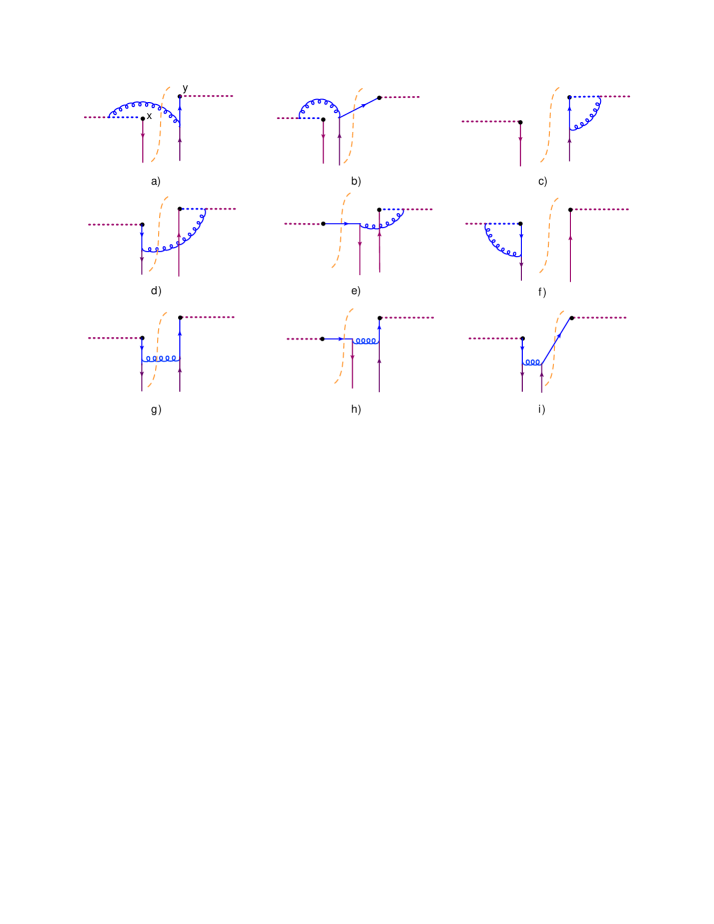
Figure 1: One-loop diagrams for TMD operator (4) in the background quark field. The dashed lines denote gauge links.

For quantum gluons, we use the background-Feynman gauge which reduces to the usual Feynman gauge in diagrams without background gluons. It is well-known that in such a gauge the contribution of the gauge link at infinity $[x_{\perp}-\infty n,y_{\perp}-\infty n]$ can be neglected, and we get diagrams shown in Fig. 1.

We will use Sudakov variables $\alpha\equiv p^{+}/{\varrho}$ and $\beta\equiv p^{-}/{\varrho}$ so that $p=\alpha p_{1}+\beta p_{2}+p_{\perp}$ where $p_{1}=n{\varrho}$ and $p_{2}$ is a lightlike vector close to $p_{B}$ so that $p_{B}=x_{B}p_{B}^{+}+p_{B_{\perp}}$. In these variables $p\cdot q~{}=~{}(\alpha_{p}\beta_{q}+\alpha_{q}\beta_{p}){s\over 2}-(p,q)_{\perp}$ where $(p,q)_{\perp}\equiv-p_{i}q^{i}$. Throughout the paper, the sum over the Latin indices $i$, $j,\dots$, runs over the two transverse components while the sum over Greek indices runs over the four components as usual.

It is convenient to define Fourier transforms of the background fields $\Psi$,

$$\Psi(\beta_{B},p_{B_{\perp}})~{}=~{}\varrho\!\int\!dz^{+}dz_{\perp}~{}\Psi(z^{+},z_{\perp})e^{i\varrho\beta_{B}z^{+}-i(p_{B},z)_{\perp}},~{}~{}~{}{\bar{\Psi}}(\beta^{\prime}_{B},p^{\prime}_{B_{\perp}})~{}=~{}\varrho\!\int\!dz^{+}dz_{\perp}~{}{\bar{\Psi}}(z^{+},z_{\perp})e^{i\varrho\beta^{\prime}_{B}z^{+}-i(p^{\prime}_{B},z)_{\perp}}$$ (10)

Hereafter we will use the notation $\beta_{B}\equiv x_{B}$ since we will calculate integrals using Sudakov variables.

Note that as discussed in Refs. Balitsky:2015qba ; Balitsky:2016dgz ; Balitsky:2017flc ; Balitsky:2017gis , in a general gauge one should replace

$$\Psi(z^{+},z_{\perp})~{}\rightarrow~{}[-\infty^{+},z^{+}]_{z}\Psi(z^{+},z_{\perp}),~{}~{}~{}~{}~{}~{}{\bar{\Psi}}(z^{+},z_{\perp})~{}\rightarrow~{}{\bar{\Psi}}(z^{+},z_{\perp})[z^{+},-\infty^{+}]_{z}$$ (11)

in the case of evolution equations for the operator (8), and

$$\Psi(z^{+},z_{\perp})~{}\rightarrow~{}[\infty^{+},z^{+}]_{z}\Psi(z^{+},z_{\perp}),~{}~{}~{}~{}~{}~{}{\bar{\Psi}}(z^{+},z_{\perp})~{}\rightarrow~{}{\bar{\Psi}}(z^{+},z_{\perp})[z^{+},\infty^{+}]_{z}$$ (12)

for evolution equations of operators (4) with gauge links out to $+\infty$.

II.2 Diagrams in Figs. 1(a)-1(c)

II.2.1 A choice of rapidity cutoff

Let us start with the diagram in Fig. 1(c) where all propagators are of Feynman type. Note that a possible diagram with Fig. 1(c) topology and with a three-gluon vertex in the left sector vanishes since the background field $\Psi(\beta_{B},p_{B_{\perp}})$ cannot produce any real particles. Also, we do not draw the diagrams with self-energy insertions in quark tails since they are not relevant for rapidity evolution. Simple calculation yields

$$\langle{\rm T}\{[-\infty,y^{+}]_{y}\Gamma\psi(y^{+},y_{\perp})\}\rangle_{\Psi}^{\rm Fig.\ref{fig:kvdiagrams}c}~{}=~{}-ig^{2}c_{F}\!\int\!{\textstyle d}\lower 0.12915pt\hbox{\kern-3.80005pt${}^{\scriptstyle-}$}\kern-0.50003pt{}\beta_{B}{\textstyle d}\lower 0.12915pt\hbox{\kern-3.80005pt${}^{\scriptstyle-}$}\kern-0.50003pt{}p_{B_{\perp}}$$

$$\times~{}e^{-ip_{B}y}\!\int\!{\textstyle d}\lower 0.12915pt\hbox{\kern-3.80005pt${}^{\scriptstyle-}$}\kern-0.50003pt{}\alpha{\textstyle d}\lower 0.12915pt\hbox{\kern-3.80005pt${}^{\scriptstyle-}$}\kern-0.50003pt{}\beta{\textstyle d}\lower 0.12915pt\hbox{\kern-3.80005pt${}^{\scriptstyle-}$}\kern-0.50003pt{}p_{\perp}{1\over\beta+{i\epsilon}}{\theta(\sigma-|\alpha|)\over\alpha\beta s-p_{\perp}^{2}+{i\epsilon}}{s(\beta-\beta_{B})\over\alpha(\beta-\beta_{B})s-(p-p_{B})_{\perp}^{2}+{i\epsilon}}\Gamma\Psi(\beta_{B},p_{B_{\perp}})$$

$$=~{}-g^{2}c_{F}\!\int\!{\textstyle d}\lower 0.12915pt\hbox{\kern-3.80005pt${}^{\scriptstyle-}$}\kern-0.50003pt{}\beta^{\prime}_{B}{\textstyle d}\lower 0.12915pt\hbox{\kern-3.80005pt${}^{\scriptstyle-}$}\kern-0.50003pt{}p_{B_{\perp}}e^{-ip_{B}y}\!\int_{0}^{\sigma}\!{\textstyle d}\lower 0.12915pt\hbox{\kern-3.80005pt${}^{\scriptstyle-}$}\kern-0.50003pt{}\alpha\!\int\!{\textstyle d}\lower 0.12915pt\hbox{\kern-3.80005pt${}^{\scriptstyle-}$}\kern-0.50003pt{}p_{\perp}{\beta_{B}s\over p_{\perp}^{2}[\alpha\beta_{B}s-(p-p_{B})_{\perp}^{2}+{i\epsilon}]}\Gamma\Psi(\beta_{B},p_{B_{\perp}})$$ (13)

Hereafter we use space-saving $\hbar$-inspired notations ${\textstyle d}\lower 0.12915pt\hbox{\kern-3.80005pt${}^{\scriptstyle-}$}\kern-0.50003pt{}^{n}p\equiv{d^{n}p\over(2\pi)^{n}}$. Note that the integral in the RHS of Eq. (13) diverges as $p_{\perp}\rightarrow 0$, but one should expect that this divergence cancels with the contribution of diagrams in Figs. 1a,b.

Next we calculate the diagrams in Figs. 1(a) and 1(b) with a combination of Feynman, complex conjugate, and cut propagators. One obtains

$$\langle[x^{+},-\infty]_{x}\Gamma\psi(y^{+},y_{\perp})\rangle_{\Psi}^{\rm Fig.\ref{fig:kvdiagrams}a,b}$$

$$=~{}g^{2}c_{F}\!\int\!{\textstyle d}\lower 0.12915pt\hbox{\kern-3.80005pt${}^{\scriptstyle-}$}\kern-0.50003pt{}\beta^{\prime}_{B}{\textstyle d}\lower 0.12915pt\hbox{\kern-3.80005pt${}^{\scriptstyle-}$}\kern-0.50003pt{}p_{B_{\perp}}e^{-i(p_{B},y)}\!\int\!{\textstyle d}\lower 0.12915pt\hbox{\kern-3.80005pt${}^{\scriptstyle-}$}\kern-0.50003pt{}\alpha{\textstyle d}\lower 0.12915pt\hbox{\kern-3.80005pt${}^{\scriptstyle-}$}\kern-0.50003pt{}\beta{\textstyle d}\lower 0.12915pt\hbox{\kern-3.80005pt${}^{\scriptstyle-}$}\kern-0.50003pt{}p_{\perp}\Big{[}2\pi\delta(\alpha(\beta-\beta_{B})s-(p-p_{B})_{\perp}^{2})(\beta-\beta_{B})s\theta(\alpha){1\over\alpha\beta s-p_{\perp}^{2}-{i\epsilon}}$$

$$\hskip 62.59605pt+~{}{(\beta-\beta_{B})s\over\alpha(\beta-\beta_{B})s-(p-p_{B})_{\perp}^{2}+{i\epsilon}}2\pi\delta(\alpha\beta s-p_{\perp}^{2})\theta(\alpha)\Big{]}{\theta(\sigma-|\alpha|)\over\beta+{i\epsilon}}e^{-i\beta{\varrho}\Delta^{+}+i(p,\Delta)_{\perp}}\Gamma\Psi(\beta_{B},p_{B_{\perp}})$$

$$=~{}g^{2}c_{F}\!\int\!{\textstyle d}\lower 0.12915pt\hbox{\kern-3.80005pt${}^{\scriptstyle-}$}\kern-0.50003pt{}\beta_{B}{\textstyle d}\lower 0.12915pt\hbox{\kern-3.80005pt${}^{\scriptstyle-}$}\kern-0.50003pt{}p_{B_{\perp}}\psi(\beta_{B},p_{B_{\perp}})e^{-ip_{B}y}\!\int_{0}^{\sigma}\!{{\textstyle d}\lower 0.12915pt\hbox{\kern-3.80005pt${}^{\scriptstyle-}$}\kern-0.50003pt{}\alpha\over\alpha}\!\int\!{\textstyle d}\lower 0.12915pt\hbox{\kern-3.80005pt${}^{\scriptstyle-}$}\kern-0.50003pt{}p_{\perp}e^{i(p,\Delta)_{\perp}}\Big{[}{(\alpha\beta_{B}s-p_{\perp}^{2})e^{-i{p_{\perp}^{2}\over\alpha s}{\varrho}\Delta^{+}}\over p_{\perp}^{2}[\alpha\beta_{B}s+(p-p_{B})_{\perp}^{2}-p_{\perp}^{2}-{i\epsilon}]}$$

$$\hskip 62.59605pt+~{}{(p-p_{B})_{\perp}^{2}e^{-i(\beta_{B}+{(p-p_{B})_{\perp}^{2}\over\alpha s}){\varrho}\Delta^{+}}\over[\alpha\beta_{B}s+(p-p_{B})_{\perp}^{2}+{i\epsilon}][\alpha\beta_{B}s+(p-p_{B})_{\perp}^{2}-p_{\perp}^{2}-{i\epsilon}]}\Big{]}\Gamma\Psi(\beta_{B},p_{B_{\perp}})$$ (14)

Hereafter we use the notation $\Delta\equiv x-y$ for brevity. The dimension of the transverse space is $d-2=2+2{\varepsilon}$ (or $d=2$ if we do not need dimensional regularization).

It is convenient to rewrite Eq. (14) as a sum of two terms

$$\langle[x^{+},-\infty]_{x}\Gamma\psi(y^{+},y_{\perp})\rangle_{\Psi}~{}=~{}\langle[x^{+},-\infty]_{x}\Gamma\psi(y^{+},y_{\perp})\rangle_{\Psi}^{(1)}+\langle[x^{+},-\infty]_{x}\Gamma\psi(y^{+},y_{\perp})\rangle_{\Psi}^{(2)}$$ (15)

where

$$\langle[x^{+},-\infty]_{x}\Gamma\psi(y^{+},y_{\perp})\rangle_{\Psi}^{(1)}~{}$$

$$\hskip 62.59605pt=~{}g^{2}c_{F}\!\int\!{\textstyle d}\lower 0.12915pt\hbox{\kern-3.80005pt${}^{\scriptstyle-}$}\kern-0.50003pt{}\beta_{B}{\textstyle d}\lower 0.12915pt\hbox{\kern-3.80005pt${}^{\scriptstyle-}$}\kern-0.50003pt{}p_{B_{\perp}}\Gamma\Psi(\beta_{B},p_{B_{\perp}})e^{-ip_{B}y}\!\int_{0}^{\sigma}\!{\textstyle d}\lower 0.12915pt\hbox{\kern-3.80005pt${}^{\scriptstyle-}$}\kern-0.50003pt{}\alpha\!\int\!{{\textstyle d}\lower 0.12915pt\hbox{\kern-3.80005pt${}^{\scriptstyle-}$}\kern-0.50003pt{}p_{\perp}\over p_{\perp}^{2}}{\beta_{B}se^{-i{p_{\perp}^{2}\over\alpha s}{\varrho}\Delta^{+}+i(p,\Delta)}\over\alpha\beta_{B}s+(p-p_{B})_{\perp}^{2}+{i\epsilon}},$$ (16)

$$\langle[x^{+},-\infty]_{x}\Gamma\psi(y^{+},y_{\perp})\rangle_{\Psi}^{(2)}~{}=~{}g^{2}c_{F}\!\int\!{\textstyle d}\lower 0.12915pt\hbox{\kern-3.80005pt${}^{\scriptstyle-}$}\kern-0.50003pt{}\beta_{B}{\textstyle d}\lower 0.12915pt\hbox{\kern-3.80005pt${}^{\scriptstyle-}$}\kern-0.50003pt{}p_{B_{\perp}}\Gamma\Psi(\beta_{B},p_{B_{\perp}})e^{-ip_{B}y}$$

$$\hskip 62.59605pt\times~{}\!\int_{0}^{\sigma}\!{{\textstyle d}\lower 0.12915pt\hbox{\kern-3.80005pt${}^{\scriptstyle-}$}\kern-0.50003pt{}\alpha\over\alpha}\!\int\!{\textstyle d}\lower 0.12915pt\hbox{\kern-3.80005pt${}^{\scriptstyle-}$}\kern-0.50003pt{}p_{\perp}{(p-p_{B})_{\perp}^{2}e^{i(p,\Delta)_{\perp}}\big{[}e^{-i(\beta_{B}+{(p-p_{B})_{\perp}^{2}\over\alpha s}){\varrho}\Delta^{+}}-e^{-i{p_{\perp}^{2}\over\alpha s}{\varrho}\Delta^{+}}\big{]}\over[\alpha\beta_{B}s+(p-p_{B})_{\perp}^{2}+{i\epsilon}][\alpha\beta_{B}s+(p-p_{B})_{\perp}^{2}-p_{\perp}^{2}]}$$ (17)

The integral in the RHS of Eq. (17) is convergent while the one in the RHS of Eq. (16) diverges as $p_{\perp}\rightarrow 0$. As we mentioned above, one should expect that this divergence cancels with the contribution (13) of diagram in Figs. 1(c). Indeed, this divergence comes from the infinite length of gauge links in Eqs. (10). As $p_{\perp}\rightarrow 0$ the integral (14) behaves in the same way as such an integral at $x_{\perp}=y_{\perp}$ so the contributions of infinite gauge links should cancel

$$\langle[x^{+},-\infty^{+}]_{y}[-\infty^{+},y^{+}]_{y}\Gamma\psi(y^{+},y_{\perp})\rangle_{\Psi}~{}=~{}\langle[x^{+},y^{+}]_{y}\Gamma\psi(y^{+},y_{\perp})\rangle_{\Psi}$$ (18)

Unfortunately, “rigid” cutoff $\sigma>|\alpha|$ does not provide this property–the sum of Eqs. (13) and (16) is still divergent as $p_{\perp}\rightarrow 0$. To ensure IR cancellations, we use a “smooth” cutoff in $\alpha$ imposed by point-splitting regularization $\psi(y^{+},y_{\perp})\rightarrow\psi(y^{+},y_{\perp},y^{-})$. We get then

$$\langle{\rm T}\{[-\infty,y^{+}]_{y}\Gamma\psi(y^{+},y_{\perp},-\delta^{-})\}\rangle_{\Psi}^{\rm Fig.\ref{fig:kvdiagrams}c}~{}=~{}-ig^{2}c_{F}\!\int\!{\textstyle d}\lower 0.12915pt\hbox{\kern-3.80005pt${}^{\scriptstyle-}$}\kern-0.50003pt{}\beta_{B}{\textstyle d}\lower 0.12915pt\hbox{\kern-3.80005pt${}^{\scriptstyle-}$}\kern-0.50003pt{}p_{B_{\perp}}$$

$$\times~{}e^{-ip_{B}y}\!\int\!{\textstyle d}\lower 0.12915pt\hbox{\kern-3.80005pt${}^{\scriptstyle-}$}\kern-0.50003pt{}\alpha{\textstyle d}\lower 0.12915pt\hbox{\kern-3.80005pt${}^{\scriptstyle-}$}\kern-0.50003pt{}\beta{\textstyle d}\lower 0.12915pt\hbox{\kern-3.80005pt${}^{\scriptstyle-}$}\kern-0.50003pt{}p_{\perp}{1\over\beta+{i\epsilon}}{e^{-i\alpha{\varrho}\delta^{-}}\over\alpha\beta s-p_{\perp}^{2}+{i\epsilon}}{s(\beta-\beta_{B})\over\alpha(\beta-\beta_{B})s-(p-p_{B})_{\perp}^{2}+{i\epsilon}}\Gamma\Psi(\beta_{B},p_{B_{\perp}})$$

$$=~{}g^{2}c_{F}\!\int\!{\textstyle d}\lower 0.12915pt\hbox{\kern-3.80005pt${}^{\scriptstyle-}$}\kern-0.50003pt{}\beta_{B}{\textstyle d}\lower 0.12915pt\hbox{\kern-3.80005pt${}^{\scriptstyle-}$}\kern-0.50003pt{}p_{B_{\perp}}e^{-ip_{B}y}\!\int_{-\infty}^{0}\!{\textstyle d}\lower 0.12915pt\hbox{\kern-3.80005pt${}^{\scriptstyle-}$}\kern-0.50003pt{}\alpha\!\int\!{\textstyle d}\lower 0.12915pt\hbox{\kern-3.80005pt${}^{\scriptstyle-}$}\kern-0.50003pt{}p_{\perp}{\beta_{B}s\over p_{\perp}^{2}[\alpha\beta_{B}s+(p-p_{B})_{\perp}^{2}-{i\epsilon}]}\Gamma\Psi(\beta_{B},p_{B_{\perp}})e^{-i{\alpha\over\sigma}}$$

$$=~{}-g^{2}c_{F}\!\int\!{\textstyle d}\lower 0.12915pt\hbox{\kern-3.80005pt${}^{\scriptstyle-}$}\kern-0.50003pt{}\beta_{B}{\textstyle d}\lower 0.12915pt\hbox{\kern-3.80005pt${}^{\scriptstyle-}$}\kern-0.50003pt{}p_{B_{\perp}}e^{-ip_{B}y}\Gamma\Psi(\beta_{B},p_{B_{\perp}})\!\int_{0}^{\infty}\!{\textstyle d}\lower 0.12915pt\hbox{\kern-3.80005pt${}^{\scriptstyle-}$}\kern-0.50003pt{}\alpha\!\int\!{\textstyle d}\lower 0.12915pt\hbox{\kern-3.80005pt${}^{\scriptstyle-}$}\kern-0.50003pt{}p_{\perp}{\beta_{B}s\over p_{\perp}^{2}[\alpha\beta_{B}s+(p-p_{B})_{\perp}^{2}+{i\epsilon}]}e^{-i{\alpha\over\sigma}}$$ (19)

where

$$\sigma\equiv{1\over{\varrho}\delta^{-}}>0.$$ (20)

Note that to get the last line in Eq. (19), we turned the contour of integration over $\alpha$ on angle $\pi$ in the lower half-plane of complex $\alpha$. At $\beta_{B}>0$ the singularity at $\alpha={(p-p_{B})_{\perp}^{2}\over\beta_{B}s}+{i\epsilon}$ does not affect the rotation, while at $\beta_{B}<0$ the rotation pushes the singularity over $\alpha$ up to $+{i\epsilon}$.

For the diagrams in Figs. 1(a) and 1(b) with point splitting one obtains

$$\langle[x^{+},-\infty]_{x}\Gamma\psi(y^{+},y_{\perp},-\delta^{-})\rangle_{\Psi}^{(1)}$$

$$\hskip 62.59605pt=~{}g^{2}c_{F}\!\int\!{\textstyle d}\lower 0.12915pt\hbox{\kern-3.80005pt${}^{\scriptstyle-}$}\kern-0.50003pt{}\beta_{B}{\textstyle d}\lower 0.12915pt\hbox{\kern-3.80005pt${}^{\scriptstyle-}$}\kern-0.50003pt{}p_{B_{\perp}}e^{-ip_{B}y}\Gamma\Psi(\beta_{B},p_{B_{\perp}})\!\int_{0}^{\infty}\!{\textstyle d}\lower 0.12915pt\hbox{\kern-3.80005pt${}^{\scriptstyle-}$}\kern-0.50003pt{}\alpha\!\int\!{{\textstyle d}\lower 0.12915pt\hbox{\kern-3.80005pt${}^{\scriptstyle-}$}\kern-0.50003pt{}p_{\perp}\over p_{\perp}^{2}}{\beta_{B}se^{-i{p_{\perp}^{2}\over\alpha s}{\varrho}\Delta^{+}+i(p,\Delta)}\over\alpha\beta_{B}s+(p-p_{B})_{\perp}^{2}+{i\epsilon}}e^{-i{\alpha\over\sigma}},$$ (21)

$$\langle[x^{+},-\infty]_{x}\Gamma\psi(y^{+},y_{\perp},-\delta^{-})\rangle_{\Psi}^{(2)}~{}=~{}g^{2}c_{F}\!\int\!{\textstyle d}\lower 0.12915pt\hbox{\kern-3.80005pt${}^{\scriptstyle-}$}\kern-0.50003pt{}\beta_{B}{\textstyle d}\lower 0.12915pt\hbox{\kern-3.80005pt${}^{\scriptstyle-}$}\kern-0.50003pt{}p_{B_{\perp}}\Gamma\Psi(\beta_{B},p_{B_{\perp}})e^{-ip_{B}y}$$

$$\hskip 62.59605pt\times~{}\!\int_{0}^{\infty}\!{{\textstyle d}\lower 0.12915pt\hbox{\kern-3.80005pt${}^{\scriptstyle-}$}\kern-0.50003pt{}\alpha\over\alpha}\!\int\!{\textstyle d}\lower 0.12915pt\hbox{\kern-3.80005pt${}^{\scriptstyle-}$}\kern-0.50003pt{}p_{\perp}{(p-p_{B})_{\perp}^{2}e^{i(p,\Delta)_{\perp}}\big{[}e^{-i(\beta_{B}+{(p-p_{B})_{\perp}^{2}\over\alpha s}){\varrho}\Delta^{+}}-e^{-i{p_{\perp}^{2}\over\alpha s}{\varrho}\Delta^{+}}\big{]}\over[\alpha\beta_{B}s+(p-p_{B})_{\perp}^{2}+{i\epsilon}][\alpha\beta_{B}s+(p-p_{B})_{\perp}^{2}-p_{\perp}^{2}]}e^{-i{\alpha\over\sigma}}$$ (22)

Now we see that the sum of Eqs. (19), (21), and (22)

$$\langle[x^{+},-\infty]_{x}[-\infty,y^{+}]_{y}\Gamma\psi(y^{+},y_{\perp},-\delta^{-})\rangle_{\Psi}^{\rm Fig.\ref{fig:kvdiagrams}a-c}$$

$$\hskip 62.59605pt=~{}g^{2}c_{F}\!\int\!{\textstyle d}\lower 0.12915pt\hbox{\kern-3.80005pt${}^{\scriptstyle-}$}\kern-0.50003pt{}\beta_{B}{\textstyle d}\lower 0.12915pt\hbox{\kern-3.80005pt${}^{\scriptstyle-}$}\kern-0.50003pt{}p_{B_{\perp}}e^{-ip_{B}y}\Gamma\Psi(\beta_{B},p_{B_{\perp}})\!\int_{0}^{\infty}\!{\textstyle d}\lower 0.12915pt\hbox{\kern-3.80005pt${}^{\scriptstyle-}$}\kern-0.50003pt{}\alpha~{}e^{-i{\alpha\over\sigma}}\!\int\!{\textstyle d}\lower 0.12915pt\hbox{\kern-3.80005pt${}^{\scriptstyle-}$}\kern-0.50003pt{}p_{\perp}~{}\bigg{(}{\beta_{B}s\big{(}e^{-i{p_{\perp}^{2}\over\alpha s}{\varrho}\Delta^{+}+i(p,\Delta)_{\perp}}-1\big{)}\over p_{\perp}^{2}[\alpha\beta_{B}s+(p-p_{B})_{\perp}^{2}+{i\epsilon}]}$$

$$\hskip 125.19212pt+~{}{(p-p_{B})_{\perp}^{2}e^{i(p,\Delta)_{\perp}}\big{[}e^{-i(\beta_{B}+{(p-p_{B})_{\perp}^{2}\over\alpha s}){\varrho}\Delta^{+}}-e^{-i{p_{\perp}^{2}\over\alpha s}{\varrho}\Delta^{+}}\big{]}\over\alpha[\alpha\beta_{B}s+(p-p_{B})_{\perp}^{2}+{i\epsilon}][\alpha\beta_{B}s+(p-p_{B})_{\perp}^{2}-p_{\perp}^{2}]}\bigg{)}$$ (23)

is given by a convergent integral. It should be emphasized that $\delta^{-}<0$; otherwise, we would not be able to make the rotation of the contour in the last line in Eq. (19) and the cancellation of IR divergences would not happen. The reason for that is that all quantum operators in $[-\infty,y^{+}]_{y}\psi(y^{+},y_{\perp})$ commute since they are on the light ray, and to preserve this commutation property [which is necessary for using Feynman propagators in Eq. (19)] we should shift $\psi(y^{+},y_{\perp})$ to a point separated by a spacelike distance from operators in the gauge link $[-\infty,y^{+}]_{y}$ (see the discussion in Appendix VII.1).

It should be emphasized that we do not suggest the nonperturbative studies of TMDs with our “point splitting” and the reason is that objects such as

$$\langle p_{N}|{\bar{\psi}}\big{(}x^{+},x_{\perp},-{1\over{\varrho}\sigma^{\prime}}\big{)}[x^{+},-\infty]_{x}[-\infty,y^{+}]_{y}\Gamma\psi\big{(}y^{+},y_{\perp},-{1\over{\varrho}\sigma}\big{)}|p_{N}\rangle$$ (24)

are meaningless since the operator is not gauge invariant. Our message is that the longitudinal integrals in the perturbative diagrams for TMDs

$$\langle p_{N}|{\bar{\psi}}\big{(}x^{+},x_{\perp}\big{)}[x^{+},-\infty]_{x}[-\infty,y^{+}]_{y}\Gamma\psi(y^{+},y_{\perp})|p_{N}\rangle$$ (25)

should be cut from above in a smooth way respecting unitarity and causality, and a mnemonic rule how to choose the proper sign of the cutoff $e^{\pm i{\alpha/\sigma}}$ is to consider the point-splitting (24). Also, the point splitting representation of rapidity cutoff in $\alpha$ helps to visualize the coordinate space approximations that we make (see Fig. 2).

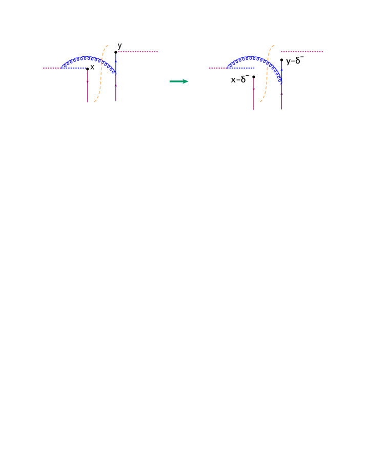
Figure 2: Point-splitting regularization of rapidity divergence.

Thus, we will be using expressions such as (24) and defining rapidity-regularized operators by

$${\bar{\psi}}^{\sigma}(x^{+},x_{\perp})~{}\equiv~{}{\bar{\psi}}\big{(}x^{+},x_{\perp},-{1\over\rho\sigma}\big{)}[x^{+},-\infty]_{x},~{}~{}~{}~{}\psi^{\sigma}(y^{+},y_{\perp})~{}\equiv~{}[-\infty,y^{+}]_{y}\psi\big{(}y^{+},y_{\perp},-{1\over\rho\sigma}\big{)},$$ (26)

but only for the perturbative calculations. In this paper we perform calculations in the (background) Feynman gauge, but in the Appendix VII.2 we demonstrate that for other gauges like Landau gauge the extra terms in gluon propagator lead to power corrections $\sim{q_{\perp}^{2}\over\beta_{B}\sigma_{t}s}\ll 1$.

It should be mentioned that the standard regularization of TMD operator (25) at moderate $x$ is a combination of UV and rapidity cutoffs, (see Ref. Collins:2011zzd ). We discuss the relation of that regularization to our rapidity-only cutoff in Appendix VII.6.

II.2.2 Rapidity evolution of diagrams in Figs. 1(a)-1(c)

In this section we will calculate the $\sigma$ dependence of the integral (23)

$$\sigma{d\over d\sigma}\!\int_{0}^{\infty}\!{\textstyle d}\lower 0.12915pt\hbox{\kern-3.80005pt${}^{\scriptstyle-}$}\kern-0.50003pt{}\alpha~{}e^{-i{\alpha\over\sigma}}\!\int\!{\textstyle d}\lower 0.12915pt\hbox{\kern-3.80005pt${}^{\scriptstyle-}$}\kern-0.50003pt{}p_{\perp}\bigg{(}{\beta_{B}s\big{(}e^{-i{p_{\perp}^{2}\over\alpha s}{\varrho}\Delta^{+}+i(p,\Delta)_{\perp}}-1\big{)}\over p_{\perp}^{2}[\alpha\beta_{B}s+(p-p_{B})_{\perp}^{2}+{i\epsilon}]}+~{}{(p-p_{B})_{\perp}^{2}e^{i(p,\Delta)_{\perp}}\big{[}e^{-i(\beta_{B}+{(p-p_{B})_{\perp}^{2}\over\alpha s}){\varrho}\Delta^{+}}-e^{-i{p_{\perp}^{2}\over\alpha s}{\varrho}\Delta^{+}}\big{]}\over\alpha[\alpha\beta_{B}s+(p-p_{B})_{\perp}^{2}+{i\epsilon}][\alpha\beta_{B}s+(p-p_{B})_{\perp}^{2}-p_{\perp}^{2}]}\bigg{)}\,.$$ (27)

First, note that the second term in the RHS does not contribute to the evolution. Indeed, characteristic $\alpha$’s in that term are $\sim{m_{\perp}^{2}\over\beta_{B}s}$ where $m_{\perp}^{2}\sim\Delta_{\perp}^{-2}\sim p_{B_{\perp}}^{2}$ so we can expand $e^{-i{\alpha\over\sigma}}$ and get approximately

$$\!\int_{0}^{\infty}\!{\textstyle d}\lower 0.12915pt\hbox{\kern-3.80005pt${}^{\scriptstyle-}$}\kern-0.50003pt{}\alpha~{}\!\int\!{\textstyle d}\lower 0.12915pt\hbox{\kern-3.80005pt${}^{\scriptstyle-}$}\kern-0.50003pt{}p_{\perp}~{}\Big{[}1-i{\alpha\over\sigma}\theta(\sigma-\alpha)\Big{]}{(p-p_{B})_{\perp}^{2}e^{i(p,\Delta)_{\perp}}\big{[}e^{-i(\beta_{B}+{(p-p_{B})_{\perp}^{2}\over\alpha s}){\varrho}\Delta^{+}}-e^{-i{p_{\perp}^{2}\over\alpha s}{\varrho}\Delta^{+}}\big{]}\over\alpha[\alpha\beta_{B}s+(p-p_{B})_{\perp}^{2}+{i\epsilon}][\alpha\beta_{B}s+(p-p_{B})_{\perp}^{2}-p_{\perp}^{2}]}\,.$$ (28)

The first term is a convergent integral independent of $\sigma$ while the second is of order of ${m_{\perp}^{2}\over\sigma\beta_{B}s}\ln{\sigma\beta_{B}s\over m_{\perp}^{2}}$ so it is a power correction that we neglect.

Next, we study the dependence of the first term in the RHS of Eq. (27) on $\Delta^{+}$. From TMD factorization (1) and definition (2) we see that we need operator (4) in the region $\Delta^{+}{\varrho}\beta_{B}\sim 1$. Let us demonstrate that in this region one can neglect $\Delta^{+}$. Indeed,

$$\!\int\!{\textstyle d}\lower 0.12915pt\hbox{\kern-3.80005pt${}^{\scriptstyle-}$}\kern-0.50003pt{}p_{\perp}~{}e^{i(p,\Delta)_{\perp}}\bigg{[}\!\int_{0}^{{p_{\perp}^{2}\over s}{\varrho}|\Delta^{+}|}\!d\alpha+\!\int_{{p_{\perp}^{2}\over s}{\varrho}|\Delta^{+}|}^{\infty}\!d\alpha\bigg{]}e^{-i{\alpha\over\sigma}}{\beta_{B}s\big{(}e^{-i{p_{\perp}^{2}\over\alpha s}{\varrho}\Delta^{+}}-1\big{)}\over p_{\perp}^{2}[\alpha\beta_{B}s+(p-p_{B})_{\perp}^{2}+{i\epsilon}]}$$ (29)

$$\simeq~{}\!\int\!{\textstyle d}\lower 0.12915pt\hbox{\kern-3.80005pt${}^{\scriptstyle-}$}\kern-0.50003pt{}p_{\perp}e^{i(p,\Delta)_{\perp}}\bigg{[}\!\int_{0}^{{p_{\perp}^{2}\over s}{\varrho}|\Delta^{+}|}\!d\alpha{\beta_{B}s\big{(}e^{-i{p_{\perp}^{2}\over\alpha s}{\varrho}\Delta^{+}}-1\big{)}\over p_{\perp}^{2}[\alpha\beta_{B}s+(p-p_{B})_{\perp}^{2}+{i\epsilon}]}-\!\int_{{p_{\perp}^{2}\over s}{\varrho}|\Delta^{+}|}^{\infty}\!{d\alpha\over\alpha}{i\beta_{B}\rho\Delta^{+}\over\alpha\beta_{B}s+(p-p_{B})_{\perp}^{2}+{i\epsilon}}\bigg{]}~{}+~{}O\big{(}{m_{\perp}^{2}\over\sigma\beta_{B}s}\big{)}$$

which is a sum of terms independent of $\sigma$ and power corrections.

Thus, we need to consider only

$$\!\int_{0}^{\infty}\!{\textstyle d}\lower 0.12915pt\hbox{\kern-3.80005pt${}^{\scriptstyle-}$}\kern-0.50003pt{}\alpha\!\int\!{{\textstyle d}\lower 0.12915pt\hbox{\kern-3.80005pt${}^{\scriptstyle-}$}\kern-0.50003pt{}p_{\perp}\over p_{\perp}^{2}}{\beta_{B}se^{-i{\alpha\over\sigma}}\big{(}e^{i(p,\Delta)_{\perp}}-1\big{)}\over\alpha\beta_{B}s+(p-p_{B})_{\perp}^{2}+{i\epsilon}}=~{}\!\int_{0}^{\infty}\!{\textstyle d}\lower 0.12915pt\hbox{\kern-3.80005pt${}^{\scriptstyle-}$}\kern-0.50003pt{}\alpha~{}e^{-i{\alpha\over\sigma}}\!\int\!{{\textstyle d}\lower 0.12915pt\hbox{\kern-3.80005pt${}^{\scriptstyle-}$}\kern-0.50003pt{}p_{\perp}\over p_{\perp}^{2}}{\beta_{B}s\big{(}e^{i(p,\Delta)_{\perp}}-1\big{)}\over\alpha\beta_{B}s+p_{\perp}^{2}+{i\epsilon}}\Big{[}1-{p_{\perp}^{2}-(p-p_{B})_{\perp}^{2}\over\alpha\beta_{B}s+(p-p_{B})_{\perp}^{2}+{i\epsilon}}\Big{]}$$

$$=~{}\!\int_{0}^{\infty}\!{\textstyle d}\lower 0.12915pt\hbox{\kern-3.80005pt${}^{\scriptstyle-}$}\kern-0.50003pt{}\alpha~{}e^{-i{\alpha\over\sigma}}\!\int\!{{\textstyle d}\lower 0.12915pt\hbox{\kern-3.80005pt${}^{\scriptstyle-}$}\kern-0.50003pt{}p_{\perp}\over p_{\perp}^{2}}{\beta_{B}s\big{(}e^{i(p,\Delta)_{\perp}}-1\big{)}\over\alpha\beta_{B}s+p_{\perp}^{2}+{i\epsilon}}~{}+~{}\!\int\!{{\textstyle d}\lower 0.12915pt\hbox{\kern-3.80005pt${}^{\scriptstyle-}$}\kern-0.50003pt{}p_{\perp}\over p_{\perp}^{2}}\big{(}e^{i(p,\Delta)_{\perp}}-1\big{)}\ln{p_{\perp}^{2}\over(p-p_{B})_{\perp}^{2}}~{}+~{}O\big{(}{m_{\perp}^{2}\over\sigma\beta_{B}s}\Big{)}$$ (30)

where we neglected the $e^{-i{\alpha\over\sigma}}$ cutoff in the second integral since it converges at $\alpha\sim{m_{\perp}^{2}\over\sigma|\beta_{B}|s}$.

The $\sigma$ dependence comes only from the first term in the RHS of Eq. (30) calculated in Appendix VII.3 [see Eq. (156)] so from Eq. (158) we get

$$\sigma{d\over d\sigma}\langle[x^{+},-\infty]_{x}[-\infty,y^{+}]_{y}\Gamma\psi(y^{+},y_{\perp},-{1\over{\varrho}\sigma})\rangle_{\Psi}$$

$$\hskip 5.69054pt=~{}-{g^{2}\over 8\pi^{2}}c_{F}\!\int\!{\textstyle d}\lower 0.12915pt\hbox{\kern-3.80005pt${}^{\scriptstyle-}$}\kern-0.50003pt{}\beta_{B}{\textstyle d}\lower 0.12915pt\hbox{\kern-3.80005pt${}^{\scriptstyle-}$}\kern-0.50003pt{}p_{B_{\perp}}\Gamma\Psi(\beta_{B},y_{\perp})e^{-ip_{B}y}\ln\Big{(}-{i\over 4}(\beta_{B}+{i\epsilon})\sigma s\Delta_{\perp}^{2}e^{\gamma}\Big{)}~{}+~{}O\big{(}{m_{\perp}^{2}\over\beta_{B}\sigma s}\big{)}$$

$$\hskip 5.69054pt=~{}-{g^{2}\over 8\pi^{2}}c_{F}\!\int\!{\textstyle d}\lower 0.12915pt\hbox{\kern-3.80005pt${}^{\scriptstyle-}$}\kern-0.50003pt{}\beta_{B}\Gamma\Psi(\beta_{B},y_{\perp})e^{-i\beta_{B}{\varrho}y^{+}}\ln\Big{(}-{i\over 4}(\beta_{B}+{i\epsilon})\sigma s\Delta_{\perp}^{2}e^{\gamma}\Big{)}~{}+~{}O\big{(}{m_{\perp}^{2}\over\beta_{B}\sigma s}\big{)}$$ (31)

where $\gamma\simeq 0.577$ is the Euler constant and $\Psi(\beta_{B},y_{\perp})={\varrho}\int\!dy^{+}e^{i\beta_{B}{\varrho}y^{+}}\Psi(y^{+},y_{\perp})$, see Eq. (10).

II.3 Diagrams in Figs. 1(d)-1(i)

The calculation of diagrams in Fig. 1(d)-1(f) repeats that of Fig. 1(a)-1(c) with minimal changes. Let us start with the diagram shown in Fig. 1f

$$\langle\tilde{\rm T}\{{\bar{\psi}}(x^{+},x_{\perp},-\delta^{-})\Gamma[x^{+},-\infty]_{x}\}\rangle_{{\bar{\Psi}}}^{\rm Fig.\ref{fig:kvdiagrams}f}~{}=~{}ig^{2}c_{F}\!\int\!{\textstyle d}\lower 0.12915pt\hbox{\kern-3.80005pt${}^{\scriptstyle-}$}\kern-0.50003pt{}\beta_{B}{\textstyle d}\lower 0.12915pt\hbox{\kern-3.80005pt${}^{\scriptstyle-}$}\kern-0.50003pt{}p_{B_{\perp}}{\bar{\Psi}}(\beta_{B},p_{B_{\perp}})\Gamma$$

$$\times~{}e^{-ip_{B}x}\!\int\!{\textstyle d}\lower 0.12915pt\hbox{\kern-3.80005pt${}^{\scriptstyle-}$}\kern-0.50003pt{}\alpha{\textstyle d}\lower 0.12915pt\hbox{\kern-3.80005pt${}^{\scriptstyle-}$}\kern-0.50003pt{}\beta{\textstyle d}\lower 0.12915pt\hbox{\kern-3.80005pt${}^{\scriptstyle-}$}\kern-0.50003pt{}p_{\perp}{1\over\beta-{i\epsilon}}{e^{-i\alpha{\varrho}\delta^{-}}\over\alpha\beta s-p_{\perp}^{2}-{i\epsilon}}{s(\beta+\beta_{B})\over\alpha(\beta+\beta_{B})s-(p+p_{B})_{\perp}^{2}-{i\epsilon}}$$

$$=~{}g^{2}c_{F}\!\int\!{\textstyle d}\lower 0.12915pt\hbox{\kern-3.80005pt${}^{\scriptstyle-}$}\kern-0.50003pt{}\beta_{B}{\textstyle d}\lower 0.12915pt\hbox{\kern-3.80005pt${}^{\scriptstyle-}$}\kern-0.50003pt{}p_{B_{\perp}}e^{-ip_{B}y}{\bar{\Psi}}(\beta_{B},p_{B_{\perp}})\Gamma\!\int_{-\infty}^{0}\!{\textstyle d}\lower 0.12915pt\hbox{\kern-3.80005pt${}^{\scriptstyle-}$}\kern-0.50003pt{}\alpha\!\int\!{\textstyle d}\lower 0.12915pt\hbox{\kern-3.80005pt${}^{\scriptstyle-}$}\kern-0.50003pt{}p_{\perp}{\beta_{B}s\over p_{\perp}^{2}[\alpha\beta_{B}s-(p+p_{B})_{\perp}^{2}-{i\epsilon}]}e^{-i{\alpha\over\sigma}}$$

$$=~{}-g^{2}c_{F}\!\int\!{\textstyle d}\lower 0.12915pt\hbox{\kern-3.80005pt${}^{\scriptstyle-}$}\kern-0.50003pt{}\beta_{B}{\textstyle d}\lower 0.12915pt\hbox{\kern-3.80005pt${}^{\scriptstyle-}$}\kern-0.50003pt{}p_{B_{\perp}}e^{-ip_{B}y}{\bar{\Psi}}(\beta_{B},p_{B_{\perp}})\Gamma\!\int_{0}^{\infty}\!{\textstyle d}\lower 0.12915pt\hbox{\kern-3.80005pt${}^{\scriptstyle-}$}\kern-0.50003pt{}\alpha\!\int\!{\textstyle d}\lower 0.12915pt\hbox{\kern-3.80005pt${}^{\scriptstyle-}$}\kern-0.50003pt{}p_{\perp}{\beta_{B}s\over p_{\perp}^{2}[\alpha\beta_{B}s-(p+p_{B})_{\perp}^{2}+{i\epsilon}]}e^{i{\alpha\over\sigma}}$$ (32)

Similar to Eq. (19), to get the last line we rotated the contour of integration over $\alpha$ in the upper half-plane of complex $\alpha$. Next, the contribution of diagrams in Figs. 1(d) and 1(e) is

$$\langle{\bar{\psi}}(x^{+},x_{\perp},-\delta^{-})[-\infty,y^{+}]_{y}\Gamma\rangle_{\Psi}^{\rm Fig.\ref{fig:kvdiagrams}d,e}~{}$$

$$=~{}g^{2}c_{F}\!\int\!{\textstyle d}\lower 0.12915pt\hbox{\kern-3.80005pt${}^{\scriptstyle-}$}\kern-0.50003pt{}\beta^{\prime}_{B}{\textstyle d}\lower 0.12915pt\hbox{\kern-3.80005pt${}^{\scriptstyle-}$}\kern-0.50003pt{}p_{B_{\perp}}e^{-i(p_{B},x)}{\bar{\Psi}}(\beta_{B},p_{B_{\perp}})\Gamma\!\int\!{\textstyle d}\lower 0.12915pt\hbox{\kern-3.80005pt${}^{\scriptstyle-}$}\kern-0.50003pt{}\alpha{\textstyle d}\lower 0.12915pt\hbox{\kern-3.80005pt${}^{\scriptstyle-}$}\kern-0.50003pt{}\beta{\textstyle d}\lower 0.12915pt\hbox{\kern-3.80005pt${}^{\scriptstyle-}$}\kern-0.50003pt{}p_{\perp}\Big{[}{1\over\alpha\beta s-p_{\perp}^{2}+{i\epsilon}}2\pi\delta(\alpha(\beta+\beta_{B})s-(p+p_{B})_{\perp}^{2})(\beta+\beta_{B})s\theta(\alpha)$$

$$\hskip 62.59605pt+~{}{(\beta+\beta_{B})s\over\alpha(\beta+\beta_{B})s-(p+p_{B})_{\perp}^{2}-{i\epsilon}}2\pi\delta(\alpha\beta s-p_{\perp}^{2})\theta(\alpha)\Big{]}{e^{i\alpha{\varrho}\delta^{-}}\over\beta-{i\epsilon}}e^{-i\beta\Delta+i(p,\Delta)_{\perp}}$$

$$=~{}g^{2}c_{F}\!\int\!{\textstyle d}\lower 0.12915pt\hbox{\kern-3.80005pt${}^{\scriptstyle-}$}\kern-0.50003pt{}\beta_{B}{\textstyle d}\lower 0.12915pt\hbox{\kern-3.80005pt${}^{\scriptstyle-}$}\kern-0.50003pt{}p_{B_{\perp}}\epsilon^{-ip_{B}x}\Gamma{\bar{\Psi}}(\beta_{B},p_{B_{\perp}})\!\int_{0}^{\infty}\!{{\textstyle d}\lower 0.12915pt\hbox{\kern-3.80005pt${}^{\scriptstyle-}$}\kern-0.50003pt{}\alpha\over\alpha}e^{i{\alpha\over\sigma}}\!\int\!{\textstyle d}\lower 0.12915pt\hbox{\kern-3.80005pt${}^{\scriptstyle-}$}\kern-0.50003pt{}p_{\perp}e^{i(p,\Delta)_{\perp}}\bigg{[}{(\alpha\beta_{B}s+p_{\perp}^{2})e^{-i{p_{\perp}^{2}\over\alpha s}{\varrho}\Delta^{+}}\over p_{\perp}^{2}[\alpha\beta_{B}s-(p+p_{B})_{\perp}^{2}+{i\epsilon}]}$$

$$\hskip 62.59605pt+~{}{(p+p_{B})_{\perp}^{2}e^{i(\beta_{B}-{(p+p_{B})_{\perp}^{2}\over\alpha s}){\varrho}\Delta^{+}}\over[\alpha\beta_{B}s-(p+p_{B})_{\perp}^{2}+{i\epsilon}][\alpha\beta_{B}s-(p+p_{B})_{\perp}^{2}+p_{\perp}^{2}]}\bigg{]}$$ (33)

The sum of Eqs. (32) and (33) can be rewritten as

$$\langle{\bar{\psi}}(x^{+},x_{\perp},-\delta^{-})[-\infty,y^{+}]_{y}\Gamma\rangle_{\Psi}^{\rm Fig.\ref{fig:kvdiagrams}d-f}~{}$$

$$=~{}g^{2}c_{F}\!\int\!{\textstyle d}\lower 0.12915pt\hbox{\kern-3.80005pt${}^{\scriptstyle-}$}\kern-0.50003pt{}\beta_{B}{\textstyle d}\lower 0.12915pt\hbox{\kern-3.80005pt${}^{\scriptstyle-}$}\kern-0.50003pt{}p_{B_{\perp}}\epsilon^{-ip_{B}x}\Gamma{\bar{\Psi}}(\beta_{B},p_{B_{\perp}})\!\int_{0}^{\infty}\!{\textstyle d}\lower 0.12915pt\hbox{\kern-3.80005pt${}^{\scriptstyle-}$}\kern-0.50003pt{}\alpha~{}e^{i{\alpha\over\sigma}}\!\int\!{\textstyle d}\lower 0.12915pt\hbox{\kern-3.80005pt${}^{\scriptstyle-}$}\kern-0.50003pt{}p_{\perp}e^{i(p,\Delta)_{\perp}}\bigg{[}{\beta_{B}s\big{(}e^{-i{p_{\perp}^{2}\over\alpha s}{\varrho}\Delta^{+}}-1\big{)}\over p_{\perp}^{2}[\alpha\beta_{B}s-(p+p_{B})_{\perp}^{2}+{i\epsilon}]}$$

$$\hskip 62.59605pt+~{}{(p+p_{B})_{\perp}^{2}\big{[}e^{i(\beta_{B}-{(p+p_{B})_{\perp}^{2}\over\alpha s}){\varrho}\Delta^{+}}-e^{-i{p_{\perp}^{2}\over\alpha s}{\varrho}\Delta^{+}}\big{]}\over\alpha[\alpha\beta_{B}s-(p+p_{B})_{\perp}^{2}+{i\epsilon}][\alpha\beta_{B}s-(p+p_{B})_{\perp}^{2}+p_{\perp}^{2}]}\bigg{]}$$ (34)

Now, the integral

$$\!\int_{0}^{\infty}\!{\textstyle d}\lower 0.12915pt\hbox{\kern-3.80005pt${}^{\scriptstyle-}$}\kern-0.50003pt{}\alpha~{}e^{i{\alpha\over\sigma}}\!\int\!{\textstyle d}\lower 0.12915pt\hbox{\kern-3.80005pt${}^{\scriptstyle-}$}\kern-0.50003pt{}p_{\perp}e^{i(p,\Delta)_{\perp}}\bigg{[}{\beta_{B}s\big{(}e^{-i{p_{\perp}^{2}\over\alpha s}{\varrho}\Delta^{+}}-1\big{)}\over p_{\perp}^{2}[\alpha\beta_{B}s-(p+p_{B})_{\perp}^{2}+{i\epsilon}]}+{(p+p_{B})_{\perp}^{2}\big{[}e^{i(\beta_{B}-{(p+p_{B})_{\perp}^{2}\over\alpha s}){\varrho}\Delta^{+}}-e^{-i{p_{\perp}^{2}\over\alpha s}{\varrho}\Delta^{+}}\big{]}\over\alpha[\alpha\beta_{B}s-(p+p_{B})_{\perp}^{2}+{i\epsilon}][\alpha\beta_{B}s-(p+p_{B})_{\perp}^{2}+p_{\perp}^{2}]}\bigg{]}$$ (35)

differs from the corresponding integral in Eq. (23) by complex conjugation and replacements $x\leftrightarrow y$, $p_{B}\leftrightarrow-p_{B}$ so we get the result obtained from Eq. (31) by the same manipulations

$$\sigma^{\prime}{d\over d\sigma^{\prime}}\langle{\bar{\psi}}(x^{+},x_{\perp},-\delta^{\prime-})\Gamma[x^{+},-\infty]_{x}[-\infty,y^{+}]_{y}\rangle_{\Psi}^{\rm Fig.\ref{fig:kvdiagrams}d-f}$$

$$\hskip 5.69054pt=~{}-{g^{2}\over 8\pi^{2}}c_{F}\!\int\!{\textstyle d}\lower 0.12915pt\hbox{\kern-3.80005pt${}^{\scriptstyle-}$}\kern-0.50003pt{}\beta_{B}{\bar{\Psi}}(\beta_{B},x_{\perp})\Gamma e^{-ip_{B}{\varrho}x^{+}}\ln\Big{(}-{i\over 4}(\beta_{B}+{i\epsilon})\sigma^{\prime}s\Delta_{\perp}^{2}e^{\gamma}\Big{)}~{}+~{}O\big{(}{m_{\perp}^{2}\over\beta_{B}\sigma^{\prime}s}\big{)}$$ (36)

Finally, let us discuss diagrams in Fig. 1(g)-1(i). Since the separation between operators ${\bar{\psi}}(x)$ and $\psi(y)$ is spacelike, we can replace the product of operators by the T-product and get

$$\langle{\rm T}\{{\bar{\psi}}(x^{+},x_{\perp},-{\delta^{\prime}}^{-})\Gamma\psi(y^{+},y_{\perp},-\delta^{-})\}\rangle_{\Psi}^{\rm Fig.\ref{fig:kvdiagrams}g-i}~{}$$ (37)

$$=~{}g^{2}c_{F}\int\!{\textstyle d}\lower 0.12915pt\hbox{\kern-3.80005pt${}^{\scriptstyle-}$}\kern-0.50003pt{}\beta_{B}\beta^{\prime}_{B}{\textstyle d}\lower 0.12915pt\hbox{\kern-3.80005pt${}^{\scriptstyle-}$}\kern-0.50003pt{}p_{B_{\perp}}{\textstyle d}\lower 0.12915pt\hbox{\kern-3.80005pt${}^{\scriptstyle-}$}\kern-0.50003pt{}p^{\prime}_{B_{\perp}}e^{-ip^{\prime}_{B}x-ip_{B}y}\!\int\!{\textstyle d}\lower 0.12915pt\hbox{\kern-3.80005pt${}^{\scriptstyle-}$}\kern-0.50003pt{}p~{}e^{i{\varrho}\alpha(\delta^{\prime}-\delta)_{-}+i{\varrho}\beta\Delta_{+}-i(p,\Delta)_{\perp}}{{\bar{\Psi}}(p_{B})\gamma_{\xi}({\not\!p}-{\not\!p}_{B})\Gamma({\not\!p}+{\not\!p}^{\prime}_{B})\gamma^{\xi}\Psi(p^{\prime}_{B})\over(p^{2}+{i\epsilon})[(p-p_{B})^{2}+{i\epsilon}][(p+p^{\prime}_{B})^{2}+{i\epsilon}]}$$

Here we introduced two different point splittings $\delta^{-}$ and ${\delta^{\prime}}^{-}$. This is a temporary auxiliary construction that simplifies solution of the differential evolution equations obtained below. In the final results we take ${\delta^{\prime}}^{-}=\delta^{-}={1\over\rho\sigma}$ where $\sigma$ is our rapidity cutoff in $\alpha$.

Let us demonstrate that the integral (37) does not depend on $\delta^{-},{\delta^{\prime}}^{-}$ in the region

$$\Delta_{\perp}^{2}\gg\Delta^{+}\delta^{-},\Delta^{+}{\delta^{\prime}}^{-}~{}~{}\Leftrightarrow~{}~{}\sigma\beta_{B}s,\sigma^{\prime}\beta_{B}s\gg m_{\perp}^{2}$$ (38)

Consider

$$\!\int\!{\textstyle d}\lower 0.12915pt\hbox{\kern-3.80005pt${}^{\scriptstyle-}$}\kern-0.50003pt{}p~{}e^{ip\cdot\tilde{\Delta}}{({\not\!p}-{\not\!p}_{B})\Gamma({\not\!p}+{\not\!p}^{\prime}_{B})\over(p^{2}+{i\epsilon})[(p-p_{B})^{2}+{i\epsilon}][(p+p^{\prime}_{B})^{2}+{i\epsilon}]}$$ (39)

$$=~{}{s\over 2}\!\int\!{\textstyle d}\lower 0.12915pt\hbox{\kern-3.80005pt${}^{\scriptstyle-}$}\kern-0.50003pt{}\alpha{\textstyle d}\lower 0.12915pt\hbox{\kern-3.80005pt${}^{\scriptstyle-}$}\kern-0.50003pt{}\beta{\textstyle d}\lower 0.12915pt\hbox{\kern-3.80005pt${}^{\scriptstyle-}$}\kern-0.50003pt{}p_{\perp}~{}e^{i\alpha{\varrho}(\delta^{\prime}-\delta)^{-}+i\beta{\varrho}\Delta^{+}}{e^{-i(p,\Delta)_{\perp}}[(\beta-\beta_{B}){\not\!p}_{2}+(p-p_{B})_{\perp}]\Gamma[(\beta+\beta^{\prime}_{B}){\not\!p}_{2}+(p+p^{\prime}_{B})_{\perp}]\over(\alpha\beta s-p_{\perp}^{2}+{i\epsilon})[\alpha(\beta-\beta_{B})s-(p-p_{B})_{\perp}^{2}+{i\epsilon}][\alpha(\beta+\beta^{\prime}_{B})s-(p+p^{\prime}_{B})_{\perp}^{2}+{i\epsilon}]}$$

where $\tilde{\Delta}=({\delta^{\prime}}^{-}-\delta^{-},\Delta^{+},\Delta_{\perp})$. Since due to Eq. (38) $\tilde{\Delta}^{2}=-\Delta_{\perp}^{2}+2\Delta^{+}(\delta-\delta^{\prime})^{-}\neq 0$, there is no overall divergence and the integral in the left-hand-side (LHS) is UV convergent. Also, since $p_{B_{\perp}},p^{\prime}_{B_{\perp}}\neq 0$ the integral in the LHS of Eq. (39) is IR convergent. Now, let us expand the RHS of this equation in powers of $(\delta-\delta^{\prime})^{-}$. The first term of the expansion is the integral (39) with $\tilde{\Delta}$ replaced by $\Delta$ which is also convergent since $\Delta^{2}=-\Delta_{\perp}^{2}<0$. Moreover, if one takes three residues over $\beta$ in the RHS [corresponding to three diagrams in Figs. 1(g), 1(h), and 1(i)] one gets integrals over $\alpha$ which converge at $\alpha\sim{m_{\perp}^{2}\over\beta_{B}s}$. Next, the integral over $\alpha$ in the second term of the expansion has an extra $\alpha$ but is still convergent so $\alpha{\varrho}(\delta^{\prime}-\delta)^{-}\sim{m_{\perp}^{2}\over\sigma\beta_{B}s}$ due to Eq. (38). Thus, the expansion of $e^{i\alpha{\varrho}(\delta^{\prime}-\delta)^{-}}$ gives the $\sigma,\sigma^{\prime}$-independent term plus power corrections that we neglect. In other words, the diagrams in Figs. 1(g)-1(i) do not contribute to the rapidity evolution in the Sudakov region.

Thus, the result of the calculation of diagrams in Fig. 1 reads

$$\Big{(}\sigma{d\over d\sigma}+\sigma^{\prime}{d\over d\sigma^{\prime}}\Big{)}\langle{\bar{\psi}}^{\sigma^{\prime}}\big{(}x^{+},x_{\perp}\big{)}[x^{+},-\infty]_{x}[-\infty,y^{+}]_{y}\Gamma\psi^{\sigma}\big{(}y^{+},y_{\perp}\big{)}\rangle_{\Psi}$$

$$\hskip 5.69054pt=~{}-{\alpha_{s}\over 2\pi}c_{F}\!\int\!{\textstyle d}\lower 0.12915pt\hbox{\kern-3.80005pt${}^{\scriptstyle-}$}\kern-0.50003pt{}\beta_{B}{\textstyle d}\lower 0.12915pt\hbox{\kern-3.80005pt${}^{\scriptstyle-}$}\kern-0.50003pt{}\beta^{\prime}_{B}{\bar{\Psi}}(\beta^{\prime}_{B},x_{\perp})\Gamma\Psi(\beta_{B},y_{\perp})e^{-i\beta^{\prime}_{B}{\varrho}x^{+}-i\beta_{B}{\varrho}y^{+}}$$

$$\hskip 5.69054pt\times~{}\Big{[}\ln\Big{(}-{i\over 4}(\beta_{B}+{i\epsilon})\sigma sb_{\perp}^{2}e^{\gamma}\Big{)}+\ln\Big{(}-{i\over 4}(\beta^{\prime}_{B}+{i\epsilon})\sigma^{\prime}sb_{\perp}^{2}e^{\gamma}\Big{)}\Big{]}~{}+~{}O\Big{(}{m_{\perp}^{2}\over\beta_{B}\sigma s},{m_{\perp}^{2}\over\beta^{\prime}_{B}\sigma^{\prime}s}\Big{)}$$ (40)

where $b_{\perp}\equiv\Delta_{\perp}$ is a standard notation for the transverse separation of the TMD operator.

II.4 Evolution equations for quark TMDs

Promoting background fields in the RHS of Eq. (40) to operators, one obtains the leading-order evolution equation of quark TMD operators in the form

$$\Big{(}\sigma{d\over d\sigma}+\sigma^{\prime}{d\over d\sigma^{\prime}}\Big{)}{\bar{\psi}}^{\sigma^{\prime}}(\beta^{\prime}_{B},x_{\perp})\Gamma\psi^{\sigma}(\beta_{B},y_{\perp})$$

$$\hskip 5.69054pt=~{}-{\alpha_{s}\over 2\pi}c_{F}{\bar{\psi}}^{\sigma^{\prime}}(\beta^{\prime}_{B},x_{\perp})\Gamma\psi^{\sigma}(\beta_{B},y_{\perp})\Big{[}\ln\Big{(}-{i\over 4}(\beta^{\prime}_{B}+{i\epsilon})\sigma^{\prime}s\Delta_{\perp}^{2}e^{\gamma}\Big{)}+\ln\Big{(}-{i\over 4}(\beta_{B}+{i\epsilon})\sigma s\Delta_{\perp}^{2}e^{\gamma}\Big{)}\Big{]}$$ (41)

where standard TMD gauge links are assumed . The solution of the evolution equation (41) reads

$${\bar{\psi}}^{\sigma^{\prime}}(\beta^{\prime}_{B},x_{\perp})\Gamma\psi^{\sigma}(\beta_{B},y_{\perp})$$ (42)

$$=~{}e^{-{\alpha_{s}c_{F}\over 4\pi}\ln{\sigma^{\prime}\over\sigma^{\prime}_{0}}\big{[}\ln{\sigma^{\prime}\sigma^{\prime}_{0}}+2\ln\big{(}-{i\over 4}(\beta^{\prime}_{B}+{i\epsilon})s\Delta_{\perp}^{2}e^{\gamma}\big{)}\big{]}}{\bar{\psi}}^{\sigma^{\prime}_{0}}(\beta^{\prime}_{B},x_{\perp})\Gamma\psi^{\sigma_{0}}(\beta_{B},y_{\perp})e^{-{\alpha_{s}c_{F}\over 4\pi}\ln{\sigma\over\sigma_{0}}\big{[}\ln{\sigma\sigma_{0}}+2\ln\big{(}-{i\over 4}(\beta^{\prime}_{B}+{i\epsilon})s\Delta_{\perp}^{2}e^{\gamma}\big{)}\big{]}}$$

It appears that two exponential factors in the RHS describe two independent evolutions of operators (26). Of course, this is not quite right since the left and right exponents come not only from “virtual” corrections of Fig. 1(c) type but also from “emission” diagrams of Fig. 1(a) and 1(b) type which is reflected in the $\Delta_{\perp}$ dependence of these factors. Still, as we will see below, this “factorized” structure persists to quark-loop corrections.

II.4.1 Leading-order evolution in the coordinate space and conformal invariance

The evolution equation in the coordinate space is easily obtained by the Fourier transformation of Eq. (41)

$$\Big{(}\sigma{d\over d\sigma}+\sigma^{\prime}{d\over d\sigma^{\prime}}\Big{)}{\bar{\psi}}^{\sigma^{\prime}}(x^{+},x_{\perp})\Gamma\psi^{\sigma}(y^{+},y_{\perp})$$

$$\hskip 5.69054pt=~{}{\alpha_{s}\over 4\pi^{2}}c_{F}\!\int\!dz^{+}~{}\Big{\{}\Big{[}i{\ln{\varrho}(-x^{+}+z^{+}+{i\epsilon})-\ln{\sigma b_{\perp}^{2}s\over 4}e^{\gamma}\over-x^{+}+z^{+}+{i\epsilon}}+{\rm c.c.}\Big{]}{\bar{\psi}}^{\sigma^{\prime}}(z^{+},x_{\perp}\big{)}\Gamma\psi^{\sigma}(y^{+},y_{\perp})$$

$$\hskip 5.69054pt+~{}\Big{[}i{\ln{\varrho}(-y^{+}+w^{+}+{i\epsilon})-\ln{\sigma^{\prime}b_{\perp}^{2}s\over 4}e^{\gamma}\over-y^{+}+w^{+}+{i\epsilon}}+{\rm c.c.}\Big{]}{\bar{\psi}}^{\sigma^{\prime}}(x^{+},x_{\perp})\Gamma\psi^{\sigma}(y^{+},y_{\perp})\Big{\}}$$ (43)

Note the “causality”: $z^{+}\leq x^{+}$ and $w^{+}\leq y^{+}$: the evolved ${\bar{\psi}}$, $\psi$ operators lag behind the original ones, similar to the case of power corrections to TMD factorization where the emission of additional projectile/target gluons also lags behind the original quark operators (see Refs. Balitsky:2017gis ; Balitsky:2020jzt ).

The solution of this equation has the form

$${\bar{\psi}}^{\sigma^{\prime}}(x^{+},x_{\perp})\Gamma\psi^{\sigma}(y^{+},y_{\perp})~{}=~{}e^{-{\alpha_{s}c_{F}\over 4\pi}\big{(}\ln{\sigma^{\prime}\over\sigma^{\prime}_{0}}\ln{\sigma^{\prime}\sigma^{\prime}_{0}}+\ln{\sigma\over\sigma_{0}}\ln{\sigma\sigma_{0}}\big{)}}$$

$$\hskip 113.81102pt\times~{}\int\!dz^{+}\bigg{[}{i\Gamma\big{(}1-{\alpha_{s}c_{F}\over 2\pi}\ln{\sigma^{\prime}\over\sigma^{\prime}_{0}}\big{)}\over(z^{+}-x^{+}+{i\epsilon})^{1-{\alpha_{s}c_{F}\over 2\pi}\ln{\sigma^{\prime}\over\sigma^{\prime}_{0}}}}+{\rm c.c.}\bigg{]}\int\!dw^{+}\bigg{[}{i\Gamma\big{(}1-{\alpha_{s}c_{F}\over 2\pi}\ln{\sigma\over\sigma_{0}}\big{)}\over(w^{+}-y^{+}+{i\epsilon})^{1-{\alpha_{s}c_{F}\over 2\pi}\ln{\sigma\over\sigma_{0}}}}+{\rm c.c.}\bigg{]}$$

$$\hskip 113.81102pt\times~{}{1\over 4\pi^{2}}\big{(}b_{\perp}^{2}e^{\gamma}\sqrt{s/8}\big{)}^{-{\alpha_{s}c_{F}\over 2\pi}\big{(}\ln{\sigma^{\prime}\over\sigma^{\prime}_{0}}+\ln{\sigma\over\sigma_{0}}\big{)}}{\bar{\psi}}^{\sigma^{\prime}_{0}}(z^{+},x_{\perp})\Gamma\psi^{\sigma_{0}}(w^{+},y_{\perp})$$ (44)

In the leading order one does not take into account QCD running coupling so one should expect some symmetries related to conformal invariance. Indeed, if we take $\sigma=\sigma^{\prime}={\varsigma\sqrt{2}\over{\varrho}|\Delta_{\perp}|}$ where $\varsigma$ is an evolution parameter, the evolution (44) is invariant under a certain subgroup of conformal group SO(2,4) (see the discussion in Ref. Balitsky:2019ayf ).

III Quark loop correction

It is well-known that the argument of the coupling constant in the LO rapidity evolution equations [(41) or (42)] cannot be determined. As we mentioned above, we will use the BLM method to fix the argument of the running coupling constant. According to the BLM procedure, we need to calculate the contribution of the first quark loop to our TMD evolution (40) and promote $-{1\over 6\pi}n_{f}$ to full $b_{0}={11\over 12\pi}N_{c}-{1\over 6\pi}n_{f}$. Each gluon propagator in diagrams in Fig. 1 should be replaced by a one-loop correction, i.e.

$${1\over p^{2}+{i\epsilon}}~{}~{} \rightarrow ~{}~{}{1\over p^{2}+{i\epsilon}}\Big{(}1+b_{0}\alpha_{s}(\mu)\ln{\tilde{\mu}^{2}\over-p^{2}-{i\epsilon}}\Big{)}$$

$${1\over p^{2}-{i\epsilon}}~{}~{} \rightarrow ~{}~{}{1\over p^{2}-{i\epsilon}}\Big{(}1+b_{0}\alpha_{s}(\mu)\ln{\tilde{\mu}^{2}\over-p^{2}+{i\epsilon}}\Big{)}$$

$$2\pi\delta(p^{2})\theta(p_{0})~{}~{} \rightarrow ~{}~{}{i\theta(p_{0})\over p^{2}+{i\epsilon}}\Big{(}1+b_{0}\alpha_{s}(\mu)\ln{\tilde{\mu}^{2}\over-p^{2}-{i\epsilon}}\Big{)}-{i\theta(p_{0})\over p^{2}-{i\epsilon}}\Big{(}1+b_{0}\alpha_{s}(\mu)\ln{\tilde{\mu}^{2}\over-p^{2}+{i\epsilon}}\Big{)}$$ (45)

where $\tilde{\mu}^{2}\equiv\bar{\mu}^{2}_{\rm MS}e^{5/3}$. The first two lines are trivial while the third line corresponds to the sum of the diagrams shown in Fig. 3.

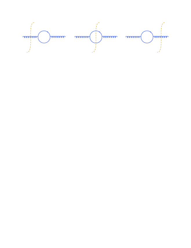
Figure 3: Quark loop correction to cut gluon propagator.

First, note that the convergence of integral (37) representing diagrams in Fig. 1(h)-1(i) is not affected by extra $\ln{\tilde{\mu}^{2}\over-p^{2}-{i\epsilon}}$. Repeating the arguments after Eq. (37) we see that the contribution of diagrams in Fig. 1(h)-1(i) with extra quark loops is still a power correction ${m_{\perp}^{2}\over\sigma\beta_{B}s}$ (multiplied by an extra log). Thus, we need to consider diagrams in Figs. 1(a)-1(c) and Figs. 1(d)-1(f).

It is convenient to start again with the diagram in Fig. 1(c). Replacing Feynman gluon propagator ${1\over p^{2}+{i\epsilon}}$ in Eq. (19) by the $\alpha_{s}$ correction from the first line in Eq. (45) we get

$$\langle{\rm T}\{[-\infty,y^{+}]_{y}\Gamma\psi(y^{+},y_{\perp},-\delta^{-})\}\rangle_{\Psi}^{\rm loop~{}1c}~{}=~{}-i4\pi b_{0}\alpha_{s}^{2}(\mu)c_{F}\!\int\!{\textstyle d}\lower 0.12915pt\hbox{\kern-3.80005pt${}^{\scriptstyle-}$}\kern-0.50003pt{}\beta_{B}{\textstyle d}\lower 0.12915pt\hbox{\kern-3.80005pt${}^{\scriptstyle-}$}\kern-0.50003pt{}p_{B_{\perp}}$$

$$\times~{}e^{-ip_{B}y}\!\int\!{\textstyle d}\lower 0.12915pt\hbox{\kern-3.80005pt${}^{\scriptstyle-}$}\kern-0.50003pt{}\alpha{\textstyle d}\lower 0.12915pt\hbox{\kern-3.80005pt${}^{\scriptstyle-}$}\kern-0.50003pt{}\beta{\textstyle d}\lower 0.12915pt\hbox{\kern-3.80005pt${}^{\scriptstyle-}$}\kern-0.50003pt{}p_{\perp}{1\over\beta+{i\epsilon}}e^{-i\alpha{\varrho}\delta^{-}}{\ln{\tilde{\mu}^{2}\over p_{\perp}^{2}-\alpha\beta s-{i\epsilon}}\over\alpha\beta s-p_{\perp}^{2}+{i\epsilon}}{s(\beta-\beta_{B})\over\alpha(\beta-\beta_{B})s-(p-p_{B})_{\perp}^{2}+{i\epsilon}}\Gamma\Psi(\beta_{B},p_{B_{\perp}})$$

$$=~{}4\pi b_{0}\alpha_{s}^{2}(\mu)c_{F}\!\int\!{\textstyle d}\lower 0.12915pt\hbox{\kern-3.80005pt${}^{\scriptstyle-}$}\kern-0.50003pt{}\beta_{B}{\textstyle d}\lower 0.12915pt\hbox{\kern-3.80005pt${}^{\scriptstyle-}$}\kern-0.50003pt{}p_{B_{\perp}}e^{-ip_{B}y}\!\int_{-\infty}^{0}\!{\textstyle d}\lower 0.12915pt\hbox{\kern-3.80005pt${}^{\scriptstyle-}$}\kern-0.50003pt{}\alpha\!\int\!{\textstyle d}\lower 0.12915pt\hbox{\kern-3.80005pt${}^{\scriptstyle-}$}\kern-0.50003pt{}p_{\perp}{\beta_{B}s\ln{\tilde{\mu}^{2}\over p_{\perp}^{2}}\over p_{\perp}^{2}[\alpha\beta_{B}s+(p-p_{B})_{\perp}^{2}-{i\epsilon}]}\Gamma\Psi(\beta_{B},p_{B_{\perp}})e^{-i{\alpha\over\sigma}}$$

$$=~{}-4\pi b_{0}\alpha_{s}^{2}(\mu)c_{F}\!\int\!{\textstyle d}\lower 0.12915pt\hbox{\kern-3.80005pt${}^{\scriptstyle-}$}\kern-0.50003pt{}\beta_{B}{\textstyle d}\lower 0.12915pt\hbox{\kern-3.80005pt${}^{\scriptstyle-}$}\kern-0.50003pt{}p_{B_{\perp}}e^{-ip_{B}y}\!\int_{0}^{\infty}\!{\textstyle d}\lower 0.12915pt\hbox{\kern-3.80005pt${}^{\scriptstyle-}$}\kern-0.50003pt{}\alpha\!\int\!{\textstyle d}\lower 0.12915pt\hbox{\kern-3.80005pt${}^{\scriptstyle-}$}\kern-0.50003pt{}p_{\perp}{\beta_{B}s\ln{\tilde{\mu}^{2}\over p_{\perp}^{2}}\over p_{\perp}^{2}[\alpha\beta_{B}s+(p-p_{B})_{\perp}^{2}+{i\epsilon}]}\Gamma\Psi(\beta_{B},p_{B_{\perp}})e^{-i{\alpha\over\sigma}}$$ (46)

where we made the same rotation of contour over $\alpha$ on angle $\pi$ in the lower complex half-plane as in Eq. (19). We get

$$\sigma{d\over d\sigma}\langle{\rm T}\{[-\infty,y^{+}]_{y}\Gamma\psi(y^{+},y_{\perp},-\delta^{-})\}\rangle_{\Psi}^{\rm loop~{}1c}$$

$$=~{}-i4\pi b_{0}\alpha_{s}^{2}(\mu)c_{F}{1\over\sigma}\!\int\!{\textstyle d}\lower 0.12915pt\hbox{\kern-3.80005pt${}^{\scriptstyle-}$}\kern-0.50003pt{}\beta_{B}{\textstyle d}\lower 0.12915pt\hbox{\kern-3.80005pt${}^{\scriptstyle-}$}\kern-0.50003pt{}p_{B_{\perp}}e^{-ip_{B}y}\!\int_{0}^{\infty}\!{\textstyle d}\lower 0.12915pt\hbox{\kern-3.80005pt${}^{\scriptstyle-}$}\kern-0.50003pt{}\alpha\!\int\!{\textstyle d}\lower 0.12915pt\hbox{\kern-3.80005pt${}^{\scriptstyle-}$}\kern-0.50003pt{}p_{\perp}{\alpha\beta_{B}s\ln{\tilde{\mu}^{2}\over p_{\perp}^{2}}\over p_{\perp}^{2}[\alpha\beta_{B}s+(p-p_{B})_{\perp}^{2}+{i\epsilon}]}\Gamma\Psi(\beta_{B},p_{B_{\perp}})e^{-i{\alpha\over\sigma}}$$ (47)

Next, consider diagrams in Figs. 1(a) and 1(b). Using Eqs. (45) for various gluon propagators, we obtain the correction in the form

$$\langle[x^{+},-\infty]_{x}\Gamma\psi(y^{+},y_{\perp},-\delta^{-})\rangle_{\Psi}^{\rm loop~{}1a,b}~{}=~{}4\pi b_{0}\alpha_{s}^{2}(\mu)c_{F}\!\int\!{\textstyle d}\lower 0.12915pt\hbox{\kern-3.80005pt${}^{\scriptstyle-}$}\kern-0.50003pt{}\beta^{\prime}_{B}{\textstyle d}\lower 0.12915pt\hbox{\kern-3.80005pt${}^{\scriptstyle-}$}\kern-0.50003pt{}p_{B_{\perp}}e^{-i(p_{B},y)}\Gamma\Psi(\beta_{B},p_{B_{\perp}})$$

$$\times~{}\!\int\!{\textstyle d}\lower 0.12915pt\hbox{\kern-3.80005pt${}^{\scriptstyle-}$}\kern-0.50003pt{}\alpha{\textstyle d}\lower 0.12915pt\hbox{\kern-3.80005pt${}^{\scriptstyle-}$}\kern-0.50003pt{}\beta{\textstyle d}\lower 0.12915pt\hbox{\kern-3.80005pt${}^{\scriptstyle-}$}\kern-0.50003pt{}p_{\perp}\bigg{[}\bigg{(}{i\theta(\alpha)\over\alpha(\beta-\beta_{B})s-(p-p_{B})_{\perp}^{2}+{i\epsilon}}-{i\theta(\alpha)\over\alpha(\beta-\beta_{B})s-(p-p_{B})_{\perp}^{2}-{i\epsilon}}\bigg{)}{(\beta-\beta_{B})\ln{\tilde{\mu}^{2}\over p_{\perp}^{2}-\alpha\beta s+{i\epsilon}}\over\alpha\beta s-p_{\perp}^{2}-{i\epsilon}}$$

$$+~{}{i(\beta-\beta_{B})s\theta(\alpha)\over\alpha(\beta-\beta_{B})s-(p-p_{B})_{\perp}^{2}+{i\epsilon}}\bigg{(}{\ln{\tilde{\mu}^{2}\over p_{\perp}^{2}-\alpha\beta s-{i\epsilon}}\over\alpha\beta s-p_{\perp}^{2}+{i\epsilon}}-{\ln{\tilde{\mu}^{2}\over p_{\perp}^{2}-\alpha\beta s+{i\epsilon}}\over\alpha\beta s-p_{\perp}^{2}-{i\epsilon}}\bigg{)}\bigg{]}{1\over\beta+{i\epsilon}}e^{-i{\alpha\over\sigma}-i\beta{\varrho}\Delta^{+}+i(p,\Delta)_{\perp}}$$

$$=~{}4\pi b_{0}\alpha_{s}^{2}(\mu)c_{F}\!\int\!{\textstyle d}\lower 0.12915pt\hbox{\kern-3.80005pt${}^{\scriptstyle-}$}\kern-0.50003pt{}\beta^{\prime}_{B}{\textstyle d}\lower 0.12915pt\hbox{\kern-3.80005pt${}^{\scriptstyle-}$}\kern-0.50003pt{}p_{B_{\perp}}e^{-i(p_{B},y)}\Gamma\Psi(\beta_{B},p_{B_{\perp}})\!\int\!{\textstyle d}\lower 0.12915pt\hbox{\kern-3.80005pt${}^{\scriptstyle-}$}\kern-0.50003pt{}\alpha{\textstyle d}\lower 0.12915pt\hbox{\kern-3.80005pt${}^{\scriptstyle-}$}\kern-0.50003pt{}\beta{\textstyle d}\lower 0.12915pt\hbox{\kern-3.80005pt${}^{\scriptstyle-}$}\kern-0.50003pt{}p_{\perp}e^{-i{\alpha\over\sigma}-i\beta{\varrho}\Delta^{+}+i(p,\Delta)_{\perp}}~{}{1\over\beta+{i\epsilon}}$$

$$\times~{}\bigg{[}{i(\beta-\beta_{B})s\theta(\alpha)\ln{\tilde{\mu}^{2}\over p_{\perp}^{2}-\alpha\beta s-{i\epsilon}}\over[\alpha(\beta-\beta_{B})s-(p-p_{B})_{\perp}^{2}+{i\epsilon}](\alpha\beta s-p_{\perp}^{2}+{i\epsilon})}-{i(\beta-\beta_{B})s\theta(\alpha)\ln{\tilde{\mu}^{2}\over p_{\perp}^{2}-\alpha\beta s+{i\epsilon}}\over[\alpha(\beta-\beta_{B})s-(p-p_{B})_{\perp}^{2}-{i\epsilon}](\alpha\beta s-p_{\perp}^{2}-{i\epsilon})}\bigg{]}\,,$$ (48)

where the second line comes from the Fig. 1(b) diagram while the third line from Fig. 1(a) diagram. The $\sigma$ evolution reads

$$\sigma{d\over d\sigma}\langle[-\infty,x^{+}]_{x}\Gamma\psi(y^{+},y_{\perp},\delta^{-})\rangle_{\Psi}^{\rm loop~{}1a,b}$$

$$=~{}i4\pi b_{0}\alpha_{s}^{2}(\mu)c_{F}{1\over\sigma}\!\int\!{\textstyle d}\lower 0.12915pt\hbox{\kern-3.80005pt${}^{\scriptstyle-}$}\kern-0.50003pt{}\beta_{B}{\textstyle d}\lower 0.12915pt\hbox{\kern-3.80005pt${}^{\scriptstyle-}$}\kern-0.50003pt{}p_{B_{\perp}}e^{-i(p_{B},y)}\Gamma\Psi(\beta_{B},p_{B_{\perp}})\!\int\!{\textstyle d}\lower 0.12915pt\hbox{\kern-3.80005pt${}^{\scriptstyle-}$}\kern-0.50003pt{}\alpha{\textstyle d}\lower 0.12915pt\hbox{\kern-3.80005pt${}^{\scriptstyle-}$}\kern-0.50003pt{}\beta{\textstyle d}\lower 0.12915pt\hbox{\kern-3.80005pt${}^{\scriptstyle-}$}\kern-0.50003pt{}p_{\perp}e^{-i{\alpha\over\sigma}-i\beta{\varrho}\Delta^{+}+i(p,\Delta)_{\perp}}~{}{1\over\beta+{i\epsilon}}$$

$$\times~{}\bigg{[}{i\alpha(\beta-\beta_{B})s\theta(\alpha)\ln{\tilde{\mu}^{2}\over p_{\perp}^{2}-\alpha\beta s-{i\epsilon}}\over[\alpha(\beta-\beta_{B})s-(p-p_{B})_{\perp}^{2}+{i\epsilon}](\alpha\beta s-p_{\perp}^{2}+{i\epsilon})}-{i\alpha(\beta-\beta_{B})s\theta(\alpha)\ln{\tilde{\mu}^{2}\over p_{\perp}^{2}-\alpha\beta s+{i\epsilon}}\over[\alpha(\beta-\beta_{B})s-(p-p_{B})_{\perp}^{2}-{i\epsilon}](\alpha\beta s-p_{\perp}^{2}-{i\epsilon})}\bigg{]}$$ (49)

Now we shall prove that the dependence of RHS on $\Delta^{+}$ is a power correction. It is convenient to consider the derivative with respect to $x^{+}$

$$\Delta^{+}{d\over dx^{+}}\sigma{d\over d\sigma}\langle[-\infty,x^{+}]_{x}\Gamma\psi(y^{+},y_{\perp},-\delta^{-})\rangle_{\Psi}^{\rm loop~{}1a,b}$$

$$=~{}4\pi b_{0}\alpha_{s}^{2}(\mu)c_{F}\!\int\!{\textstyle d}\lower 0.12915pt\hbox{\kern-3.80005pt${}^{\scriptstyle-}$}\kern-0.50003pt{}\beta^{\prime}_{B}{\textstyle d}\lower 0.12915pt\hbox{\kern-3.80005pt${}^{\scriptstyle-}$}\kern-0.50003pt{}p_{B_{\perp}}e^{-i(p_{B},y)}\Gamma\Psi(\beta_{B},p_{B_{\perp}}){{\varrho}\Delta^{+}\over\sigma}\!\int\!{\textstyle d}\lower 0.12915pt\hbox{\kern-3.80005pt${}^{\scriptstyle-}$}\kern-0.50003pt{}\alpha{\textstyle d}\lower 0.12915pt\hbox{\kern-3.80005pt${}^{\scriptstyle-}$}\kern-0.50003pt{}\beta{\textstyle d}\lower 0.12915pt\hbox{\kern-3.80005pt${}^{\scriptstyle-}$}\kern-0.50003pt{}p_{\perp}e^{-i{\alpha\over\sigma}-i\beta{\varrho}\Delta^{+}+i(p,\Delta)_{\perp}}~{}$$

$$\times\bigg{[}{i\alpha(\beta-\beta_{B})s\theta(\alpha)\ln{\tilde{\mu}^{2}\over p_{\perp}^{2}-\alpha\beta s-{i\epsilon}}\over[\alpha(\beta-\beta_{B})s-(p-p_{B})_{\perp}^{2}+{i\epsilon}](\alpha\beta s-p_{\perp}^{2}+{i\epsilon})}-{i\alpha(\beta-\beta_{B})s\theta(\alpha)\ln{\tilde{\mu}^{2}\over p_{\perp}^{2}-\alpha\beta s+{i\epsilon}}\over[\alpha(\beta-\beta_{B})s-(p-p_{B})_{\perp}^{2}-{i\epsilon}](\alpha\beta s-p_{\perp}^{2}-{i\epsilon})}\bigg{]}$$ (50)

Let us consider case $\Delta^{+}>0$. The second term in the square brackets in the RHS of Eq. (50) vanishes while the first one can be rewritten as

$${{\varrho}\Delta^{+}\over\sigma}\!\int\!{\textstyle d}\lower 0.12915pt\hbox{\kern-3.80005pt${}^{\scriptstyle-}$}\kern-0.50003pt{}\alpha{\textstyle d}\lower 0.12915pt\hbox{\kern-3.80005pt${}^{\scriptstyle-}$}\kern-0.50003pt{}\beta{\textstyle d}\lower 0.12915pt\hbox{\kern-3.80005pt${}^{\scriptstyle-}$}\kern-0.50003pt{}p_{\perp}e^{-i{\alpha\over\sigma}-i\beta{\varrho}\Delta^{+}+i(p,\Delta)_{\perp}}~{}{i\alpha(\beta-\beta_{B})s\theta(\alpha)\ln{\tilde{\mu}^{2}\over p_{\perp}^{2}-\alpha\beta s-{i\epsilon}}\over[\alpha(\beta-\beta_{B})s-(p-p_{B})_{\perp}^{2}+{i\epsilon}](\alpha\beta s-p_{\perp}^{2}+{i\epsilon})}$$ (51)

$$=~{}{{\varrho}\Delta^{+}\over\sigma}\!\int\!{\textstyle d}\lower 0.12915pt\hbox{\kern-3.80005pt${}^{\scriptstyle-}$}\kern-0.50003pt{}\alpha{\textstyle d}\lower 0.12915pt\hbox{\kern-3.80005pt${}^{\scriptstyle-}$}\kern-0.50003pt{}\beta{\textstyle d}\lower 0.12915pt\hbox{\kern-3.80005pt${}^{\scriptstyle-}$}\kern-0.50003pt{}p_{\perp}e^{-i{\alpha\over\sigma}-i\beta{\varrho}\Delta^{+}+i(p,\Delta)_{\perp}}~{}\theta(\alpha)\bigg{[}{\ln{\tilde{\mu}^{2}\over p_{\perp}^{2}-\alpha\beta s-{i\epsilon}}\over\alpha\beta s-p_{\perp}^{2}+{i\epsilon}}+{i(p-p_{B})_{\perp}^{2}\ln{\tilde{\mu}^{2}\over p_{\perp}^{2}-\alpha\beta s-{i\epsilon}}\over[\alpha(\beta-\beta_{B})s-(p-p_{B})_{\perp}^{2}+{i\epsilon}](\alpha\beta s-p_{\perp}^{2}+{i\epsilon})}\bigg{]}$$

The first term in the RHS can easily be calculated

$${2{\varrho}\Delta^{+}\over\sigma s}\!\int{\textstyle d}\lower 0.12915pt\hbox{\kern-3.80005pt${}^{\scriptstyle-}$}\kern-0.50003pt{}^{4}p~{}{\ln{\tilde{\mu}^{2}\over-p^{2}-{i\epsilon}}\over p^{2}+{i\epsilon}}e^{-ip\cdot\tilde{\Delta}}~{}=~{}{2\beta_{B}{\varrho}\Delta^{+}\over\sigma\beta_{B}s}{\ln(-\tilde{\Delta}^{2}\mu^{2}+{i\epsilon})\over 4\pi^{2}(-\tilde{\Delta}^{2}+{i\epsilon})}~{}\simeq~{}{2\beta_{B}{\varrho}\Delta^{+}\over\sigma\beta_{B}s}{\ln(\Delta_{\perp}^{2}\mu^{2}+{i\epsilon})\over 4\pi^{2}\Delta_{\perp}^{2}}~{}\sim~{}\beta_{B}{\varrho}\Delta^{+}\times O\Big{(}{m_{\perp}^{2}\over\sigma\beta_{B}s}\Big{)}$$ (52)

where $\tilde{\Delta}^{2}=-2\Delta^{+}\delta^{-}-\Delta_{\perp}^{2}\simeq-\Delta_{\perp}^{2}$. Since, as discussed in the Introduction, we consider $\beta{\varrho}\Delta^{+}\sim 1$, this term is a power correction $\sim{m_{\perp}^{2}\over\sigma\beta_{B}s}$. As to the second term in the RHS of Eq. (51), it can be estimated as follows: since the integral over $p_{\perp}$ is convergent at $p_{\perp}\sim\Delta_{\perp}^{-1}\sim m_{\perp}$, one can replace $(p-p_{B})_{\perp}^{2}$ in the numerator approximately by $m_{\perp}^{2}$ and get

$${\varrho}\Delta^{+}{2m_{\perp}^{2}\over\sigma s}\!\int{\textstyle d}\lower 0.12915pt\hbox{\kern-3.80005pt${}^{\scriptstyle-}$}\kern-0.50003pt{}^{4}p~{}{\ln{\tilde{\mu}^{2}\over-p^{2}-{i\epsilon}}\over(p^{2}+{i\epsilon})[(p-p_{B})_{\perp}^{2}+{i\epsilon}]}e^{-ip\cdot\tilde{\Delta}}~{}\sim~{}\beta_{B}{\varrho}\Delta^{+}O\Big{(}{m_{\perp}^{2}\over\sigma\beta_{B}s}\Big{)}$$ (53)

Indeed, the integral over momenta in the RHS. can be represented as (${\bar{u}}\equiv 1-u$)

$$\!\int{{\textstyle d}\lower 0.12915pt\hbox{\kern-3.80005pt${}^{\scriptstyle-}$}\kern-0.50003pt{}^{4}p\over i}~{}{\ln{\tilde{\mu}^{2}\over-p^{2}-{i\epsilon}}\over(p^{2}+{i\epsilon})[(p-p_{B})_{\perp}^{2}+{i\epsilon}]}e^{-ip\cdot\tilde{\Delta}}~{}=~{}\int_{0}^{1}\!du~{}e^{iu(p_{B}\cdot\Delta)_{\perp}}\!\int{{\textstyle d}\lower 0.12915pt\hbox{\kern-3.80005pt${}^{\scriptstyle-}$}\kern-0.50003pt{}^{4}p\over i}e^{-ip\cdot\tilde{\Delta}}{1+\ln{\bar{u}}-\ln(p_{B_{\perp}}^{2}{\bar{u}}u-p^{2}-{i\epsilon})/\tilde{\mu}^{2}\over(p_{B_{\perp}}^{2}{\bar{u}}u-p^{2}-{i\epsilon})^{2}}$$

$$\simeq~{}{1\over 16\pi^{2}}\!\int_{0}^{1}\!du~{}e^{iu(p_{B},\Delta)_{\perp}}\Big{(}\ln{\Delta_{\perp}^{2}\tilde{\mu}^{2}\over 4}-\ln{p_{B_{\perp}}^{2}\over\mu^{2}}+2\gamma+\ln{{\bar{u}}\over u}\Big{)}K_{0}\big{(}\sqrt{p_{B_{\perp}}^{2}\Delta_{\perp}^{2}{\bar{u}}u}\big{)}$$ (54)

where we used $\tilde{\Delta}^{2}\simeq-\Delta_{\perp}^{2}$. This integral is obviously $O(1)$ at $p_{B_{\perp}}^{2}\sim\Delta_{\perp}^{-2}\sim m_{\perp}^{2}$.

Summarizing, we proved that at $\Delta^{+}>0$ the RHS of integral (50) is a power correction. Also, at $\Delta^{+}<0$ only the second term in square brackets in the RHS of integral (50) contributes, and similar calculation shows that Eq. (50) is a power correction. Thus, with power accuracy $O\Big{(}{m_{\perp}^{2}\over\sigma\beta_{B}s}\Big{)}$ we can set $\Delta^{+}=0$.

Returning to Eq. (49) and taking $\Delta^{+}=0$ we get

$$\sigma{d\over d\sigma}\langle[-\infty,x^{+}]_{x}\Gamma\psi(y^{+},y_{\perp},-\delta^{-})\rangle_{\Psi}^{\rm loop~{}1a,b}$$

$$=~{}i4\pi b_{0}\alpha_{s}^{2}(\mu)c_{F}{1\over\sigma}\!\int\!{\textstyle d}\lower 0.12915pt\hbox{\kern-3.80005pt${}^{\scriptstyle-}$}\kern-0.50003pt{}\beta^{\prime}_{B}{\textstyle d}\lower 0.12915pt\hbox{\kern-3.80005pt${}^{\scriptstyle-}$}\kern-0.50003pt{}p_{B_{\perp}}e^{-i(p_{B},y)}\Gamma\Psi(\beta_{B},p_{B_{\perp}})\!\int\!{\textstyle d}\lower 0.12915pt\hbox{\kern-3.80005pt${}^{\scriptstyle-}$}\kern-0.50003pt{}\alpha{\textstyle d}\lower 0.12915pt\hbox{\kern-3.80005pt${}^{\scriptstyle-}$}\kern-0.50003pt{}\beta{\textstyle d}\lower 0.12915pt\hbox{\kern-3.80005pt${}^{\scriptstyle-}$}\kern-0.50003pt{}p_{\perp}e^{-i{\alpha\over\sigma}+i(p,\Delta)_{\perp}}~{}{1\over\beta+{i\epsilon}}$$

$$\times\bigg{[}{i\alpha(\beta-\beta_{B})s\theta(\alpha)\ln{\tilde{\mu}^{2}\over p_{\perp}^{2}-\alpha\beta s-{i\epsilon}}\over[\alpha(\beta-\beta_{B})s-(p-p_{B})_{\perp}^{2}+{i\epsilon}](\alpha\beta s-p_{\perp}^{2}+{i\epsilon})}-{i\alpha(\beta-\beta_{B})s\theta(\alpha)\ln{\tilde{\mu}^{2}\over p_{\perp}^{2}-\alpha\beta s+{i\epsilon}}\over[\alpha(\beta-\beta_{B})s-(p-p_{B})_{\perp}^{2}-{i\epsilon}](\alpha\beta s-p_{\perp}^{2}-{i\epsilon})}\bigg{]}$$

$$=~{}i4\pi b_{0}\alpha_{s}^{2}(\mu)c_{F}{1\over\sigma}\!\int\!{\textstyle d}\lower 0.12915pt\hbox{\kern-3.80005pt${}^{\scriptstyle-}$}\kern-0.50003pt{}\beta_{B}{\textstyle d}\lower 0.12915pt\hbox{\kern-3.80005pt${}^{\scriptstyle-}$}\kern-0.50003pt{}p_{B_{\perp}}e^{-ip_{B}y}\Gamma\Psi(\beta_{B},p_{B_{\perp}})\!\int_{0}^{\infty}\!{\textstyle d}\lower 0.12915pt\hbox{\kern-3.80005pt${}^{\scriptstyle-}$}\kern-0.50003pt{}\alpha\!\int\!{\textstyle d}\lower 0.12915pt\hbox{\kern-3.80005pt${}^{\scriptstyle-}$}\kern-0.50003pt{}p_{\perp}{\alpha\beta_{B}s\ln{\tilde{\mu}^{2}\over p_{\perp}^{2}}\over p_{\perp}^{2}[\alpha\beta_{B}s+(p-p_{B})_{\perp}^{2}+{i\epsilon}]}e^{-i{\alpha\over\sigma}}$$ (55)

The total contribution of diagrams in Figs. 1(a)-1(c) is a sum of Eqs. (47) and (55)

$$\sigma{d\over d\sigma}\langle[-\infty,y^{+}]_{y}\Gamma\psi(y^{+},y_{\perp},-\delta^{-})\rangle_{\Psi}^{\rm Fig1a-c~{}loop}$$

$$=~{}i4\pi b_{0}\alpha_{s}^{2}(\mu)c_{F}\!\int\!{\textstyle d}\lower 0.12915pt\hbox{\kern-3.80005pt${}^{\scriptstyle-}$}\kern-0.50003pt{}\beta_{B}{\textstyle d}\lower 0.12915pt\hbox{\kern-3.80005pt${}^{\scriptstyle-}$}\kern-0.50003pt{}p_{B_{\perp}}e^{-ip_{B}y}\Gamma\Psi(\beta_{B},p_{B_{\perp}})\!\int_{0}^{\infty}\!{{\textstyle d}\lower 0.12915pt\hbox{\kern-3.80005pt${}^{\scriptstyle-}$}\kern-0.50003pt{}\alpha\over\sigma}e^{-i{\alpha\over\sigma}}\!\int\!{\textstyle d}\lower 0.12915pt\hbox{\kern-3.80005pt${}^{\scriptstyle-}$}\kern-0.50003pt{}p_{\perp}{\big{(}e^{i(p,\Delta)_{\perp}}-1\big{)}\alpha\beta_{B}s\ln{\tilde{\mu}^{2}\over p_{\perp}^{2}}\over p_{\perp}^{2}[\alpha\beta_{B}s+(p-p_{B})_{\perp}^{2}+{i\epsilon}]}$$ (56)

Next, similar to Eq. (30) one can demonstrate that $p_{B_{\perp}}$ dependence in the integral in the RHS can be omitted with power accuracy. Indeed,

$$\!\int_{0}^{\infty}\!{{\textstyle d}\lower 0.12915pt\hbox{\kern-3.80005pt${}^{\scriptstyle-}$}\kern-0.50003pt{}\alpha\over\sigma}e^{-i{\alpha\over\sigma}}\!\int\!{\textstyle d}\lower 0.12915pt\hbox{\kern-3.80005pt${}^{\scriptstyle-}$}\kern-0.50003pt{}p_{\perp}\big{(}e^{i(p,\Delta)_{\perp}}-1\big{)}\alpha\beta_{B}s\ln{\tilde{\mu}^{2}\over p_{\perp}^{2}}\Big{[}{1\over\alpha\beta_{B}s+(p-p_{B})_{\perp}^{2}+{i\epsilon}}-{1\over\alpha\beta_{B}s+p_{\perp}^{2}+{i\epsilon}}\Big{]}$$ (57)

$$\simeq~{}\!\int\!{\textstyle d}\lower 0.12915pt\hbox{\kern-3.80005pt${}^{\scriptstyle-}$}\kern-0.50003pt{}p_{\perp}\big{(}e^{i(p,\Delta)_{\perp}}-1\big{)}\ln{\tilde{\mu}^{2}\over p_{\perp}^{2}}\!\int_{0}^{\sigma}\!{{\textstyle d}\lower 0.12915pt\hbox{\kern-3.80005pt${}^{\scriptstyle-}$}\kern-0.50003pt{}\alpha\over\sigma}\Big{[}{p_{\perp}^{2}\over\alpha\beta_{B}s+p_{\perp}^{2}+{i\epsilon}}-{(p-p_{B})_{\perp}^{2}\over\alpha\beta_{B}s+(p-p_{B})_{\perp}^{2}+{i\epsilon}}\Big{]}$$

$$=~{}{1\over 2\pi}\!\int\!{\textstyle d}\lower 0.12915pt\hbox{\kern-3.80005pt${}^{\scriptstyle-}$}\kern-0.50003pt{}p_{\perp}\big{(}1-e^{i(p,\Delta)_{\perp}}\big{)}\ln{\tilde{\mu}^{2}\over p_{\perp}^{2}}\Big{[}{(p-p_{B})_{\perp}^{2}\over\sigma\beta_{B}s}\ln{\sigma\beta_{B}s+(p-p_{B})_{\perp}^{2}+{i\epsilon}\over(p-p_{B})_{\perp}^{2}}-(p_{B_{\perp}}\rightarrow 0)\Big{]}~{}\sim~{}O\Big{(}{m_{\perp}^{2}\over\sigma\beta_{B}s}\ln{\sigma\beta_{B}s\over m_{\perp}^{2}}\Big{)}$$

Thus, we get

$$\sigma{d\over d\sigma}\langle[-\infty,y^{+}]_{y}\Gamma\psi(y^{+},y_{\perp},-\delta^{-})\rangle_{\Psi}^{\rm Fig1a-c~{}loop}$$

$$=~{}i4\pi b_{0}\alpha_{s}^{2}(\tilde{\mu})c_{F}\!\int\!{\textstyle d}\lower 0.12915pt\hbox{\kern-3.80005pt${}^{\scriptstyle-}$}\kern-0.50003pt{}\beta_{B}{\textstyle d}\lower 0.12915pt\hbox{\kern-3.80005pt${}^{\scriptstyle-}$}\kern-0.50003pt{}p_{B_{\perp}}e^{-ip_{B}y}\Gamma\Psi(\beta_{B},p_{B_{\perp}})\!\int_{0}^{\infty}\!{{\textstyle d}\lower 0.12915pt\hbox{\kern-3.80005pt${}^{\scriptstyle-}$}\kern-0.50003pt{}\alpha\over\sigma}e^{-i{\alpha\over\sigma}}\!\int\!{\textstyle d}\lower 0.12915pt\hbox{\kern-3.80005pt${}^{\scriptstyle-}$}\kern-0.50003pt{}p_{\perp}{\big{(}e^{i(p,\Delta)_{\perp}}-1\big{)}\alpha\beta_{B}s\ln{\tilde{\mu}^{2}\over p_{\perp}^{2}}\over p_{\perp}^{2}[\alpha\beta_{B}s+p_{\perp}^{2}+{i\epsilon}]}$$ (58)

The integral in the RHS of this equation is calculated in Appendix VII.3 [see Eq. (161)], so we get the result with one-loop accuracy in the form

$$\sigma{d\over d\sigma}\langle[x^{+},-\infty]_{x}[-\infty,y^{+}]_{y}\Gamma\psi(y^{+},y_{\perp},-\delta^{-})\rangle_{\Psi}^{\rm Fig1a-c~{}loop}$$ (59)

$$\hskip 5.69054pt=~{}-{\alpha_{s}(\tilde{\mu})\over 2\pi}c_{F}\!\int\!{\textstyle d}\lower 0.12915pt\hbox{\kern-3.80005pt${}^{\scriptstyle-}$}\kern-0.50003pt{}\beta_{B}{\textstyle d}\lower 0.12915pt\hbox{\kern-3.80005pt${}^{\scriptstyle-}$}\kern-0.50003pt{}p_{B_{\perp}}\Gamma\Psi(\beta_{B},p_{B_{\perp}})e^{-ip_{B}y}\Big{\{}\ln\big{[}-{i\over 4}(\beta_{B}+{i\epsilon})\sigma s\Delta_{\perp}^{2}e^{\gamma}\big{]}$$

$$\hskip 5.69054pt+~{}{b_{0}\over 2}\alpha_{s}(\tilde{\mu})\Big{[}\big{(}\ln{\Delta_{\perp}^{2}\tilde{\mu}^{4}/4\over-i\sigma(\beta_{B}+{i\epsilon})s}+3\gamma\big{)}\ln\big{[}-{i\over 4}(\beta_{B}+{i\epsilon})\sigma s\Delta_{\perp}^{2}e^{\gamma}\big{]}-{\pi^{2}\over 2}\Big{]}\Big{\}}~{}+~{}O\big{(}{m_{\perp}^{2}\over\beta_{B}\sigma s}\big{)}$$

$$\hskip 5.69054pt=~{}-{\alpha_{s}(\mu_{\sigma})\over 2\pi}c_{F}\!\int\!{\textstyle d}\lower 0.12915pt\hbox{\kern-3.80005pt${}^{\scriptstyle-}$}\kern-0.50003pt{}\beta_{B}\Gamma\Psi(\beta_{B},y_{\perp})e^{-i\beta_{B}{\varrho}y^{+}}\big{\{}\ln\big{[}-{i\over 4}(\beta_{B}+{i\epsilon})\sigma s\Delta_{\perp}^{2}e^{\gamma}\big{]}+O\big{(}\alpha_{s}(\mu_{\sigma})\big{)}\big{\}}~{}+~{}O\big{(}{m_{\perp}^{2}\over\beta_{B}\sigma s}\big{)}$$

where $\mu^{2}_{\sigma}\equiv\sqrt{\sigma|\beta_{B}|s\over\Delta_{\perp}^{2}}$. Thus, the BLM scale for Sudakov evolution is halfway between the transverse momentum and the energy scale of TMD.

Performing a similar calculation of the loop contribution to diagrams in Figs. 1(d)-1(f) we obtain

$$\sigma^{\prime}{d\over d\sigma^{\prime}}\langle{\bar{\psi}}(x^{+},x_{\perp},-{\delta^{\prime}}^{-})\Gamma[x^{+},-\infty]_{x}[-\infty,y^{+}]_{y}\rangle_{\Psi}^{\rm Fig1d-f}$$ (60)

$$\hskip 5.69054pt=~{}-{\alpha_{s}(\mu^{\prime}_{\sigma})\over 2\pi}c_{F}\!\int\!{\textstyle d}\lower 0.12915pt\hbox{\kern-3.80005pt${}^{\scriptstyle-}$}\kern-0.50003pt{}\beta^{\prime}_{B}\Gamma{\bar{\Psi}}(\beta^{\prime}_{B},x_{\perp})e^{-i\beta^{\prime}_{B}{\varrho}x^{+}}\big{\{}\ln\big{[}-{i\over 4}(\beta^{\prime}_{B}+{i\epsilon})\sigma^{\prime}s\Delta_{\perp}^{2}e^{\gamma}\big{]}+O\big{(}(\alpha_{s}(\mu^{\prime}_{\sigma})\big{)}]\big{\}}~{}+~{}O\big{(}{m_{\perp}^{2}\over\beta_{B}\sigma^{\prime}s}\big{)}$$

where $\mu^{2}_{\sigma^{\prime}}\equiv\sqrt{\sigma^{\prime}|\beta^{\prime}_{B}|s\over\Delta_{\perp}^{2}}$.

Combining Eqs. (59), (60) and promoting background fields to operators we obtain the evolution equation for the TMD operator in the form

$$\Big{(}\sigma{d\over d\sigma}+\sigma^{\prime}{d\over d\sigma^{\prime}}\Big{)}{\bar{\psi}}^{\sigma^{\prime}}(\beta^{\prime}_{B},x_{\perp})\Gamma\psi^{\sigma}(\beta_{B},y_{\perp})$$ (61)

$$\hskip 5.69054pt=~{}-{c_{F}\over 2\pi}{\bar{\psi}}^{\sigma^{\prime}}(\beta^{\prime}_{B},x_{\perp})\Gamma\psi^{\sigma}(\beta_{B},y_{\perp})\Big{[}\alpha_{s}(\mu_{\sigma^{\prime}})\ln\Big{(}-{i\over 4}(\beta^{\prime}_{B}+{i\epsilon})\sigma^{\prime}sb_{\perp}^{2}e^{\gamma}\Big{)}+\alpha_{s}(\mu_{\sigma})\ln\Big{(}-{i\over 4}(\beta_{B}+{i\epsilon})\sigma sb_{\perp}^{2}e^{\gamma}\Big{)}\Big{]}$$

where $b_{\perp}\equiv\Delta_{\perp}=(x-y)_{\perp}$ We see that in the Sudakov region we can define TMD operator (4) with two independent “left” and “right” cutoffs $\sigma$ and $\sigma^{\prime}$ defined in Eqs. (26) and the evolutions with respect to those cutoffs are independent [except for $b_{\perp}=(x-y)_{\perp}$].

We can solve evolution equation (61) by replacing $\sigma{d\over d\sigma}=-{b_{0}\over 2}\alpha^{2}(\mu_{\sigma}){d\over d\alpha(\mu_{\sigma})}$ (and similarly for $\sigma^{\prime}{d\over d\sigma^{\prime}}$). We get then

$$\Big{(}\alpha^{2}(\mu_{\sigma}){d\over d\alpha(\mu_{\sigma})}+\alpha^{2}(\mu_{\sigma^{\prime}}){d\over d\alpha(\mu_{\sigma^{\prime}})}\Big{)}{\bar{\psi}}^{\sigma^{\prime}}(\beta^{\prime}_{B},x_{\perp})\Gamma\psi^{\sigma}(\beta_{B},y_{\perp})$$ (62)

$$=~{}{c_{F}\over\pi b_{0}}\Big{[}\alpha_{s}(\mu_{\sigma^{\prime}})\ln\Big{(}-{i\over 4}(\beta^{\prime}_{B}+{i\epsilon})\sigma^{\prime}sb_{\perp}^{2}e^{\gamma}\Big{)}+\alpha_{s}(\mu_{\sigma})\ln\Big{(}-{i\over 4}(\beta_{B}+{i\epsilon})\sigma sb_{\perp}^{2}e^{\gamma}\Big{)}\Big{]}{\bar{\psi}}^{\sigma^{\prime}}(\beta^{\prime}_{B},x_{\perp})\Gamma\psi^{\sigma}(\beta_{B},y_{\perp})$$

$$=~{}-{2c_{F}\over\pi b_{0}^{2}}\Big{\{}{\alpha_{s}(\mu_{\sigma^{\prime}})\over\alpha_{s}(\tilde{b}_{\perp}^{-1})}+{\alpha_{s}(\mu_{\sigma})\over\alpha_{s}(\tilde{b}_{\perp}^{-1})}-2-{b_{0}\alpha_{s}(\mu_{\sigma^{\prime}})\over 2}\ln[-i(\tau^{\prime}_{B}+{i\epsilon})]-{b_{0}\alpha_{s}(\mu_{\sigma})\over 2}\ln[-i(\tau_{B}+{i\epsilon})]\Big{\}}{\bar{\psi}}^{\sigma^{\prime}}(\beta^{\prime}_{B},x_{\perp})\Gamma\psi^{\sigma}(\beta_{B},y_{\perp})$$

where $\tilde{b}_{\perp}^{2}={b_{\perp}^{2}\over 2}e^{\gamma/2}$ and $\tau_{B}={\beta_{B}\over|\beta_{B}|},\tau^{\prime}_{B}={\beta^{\prime}_{B}\over|\beta^{\prime}_{B}|}$. Note that formally $\alpha_{s}\ln[-i(\tau_{B}+{i\epsilon})]$ exceeds our accuracy but we keep to ensure the correct causal structure in the coordinate space, similar to the leading order evolution (43).

The solution of Eq. (61) has the form

$${\bar{\psi}}^{\sigma^{\prime}}(\beta^{\prime}_{B},x_{\perp})\Gamma\psi^{\sigma}(\beta_{B},y_{\perp})~{}=~{}e^{-{2c_{F}\over\pi b_{0}^{2}}\big{[}\big{(}{1\over\alpha_{s}(\tilde{b}_{\perp}^{-1})}-{b_{0}\over 2}\ln[-i(\tau^{\prime}_{B}+{i\epsilon})]\big{)}\ln{\alpha_{s}(\mu_{\sigma^{\prime}})\over\alpha_{s}(\mu_{\sigma^{\prime}_{0}})}+{1\over\alpha_{s}(\mu_{\sigma^{\prime}})}-{1\over\alpha_{s}(\mu_{\sigma^{\prime}_{0}})}\big{]}}$$

$$\times~{}e^{-{2c_{F}\over\pi b_{0}^{2}}\big{[}\big{(}{1\over\alpha_{s}(\tilde{b}_{\perp}^{-1})}-{b_{0}\over 2}\ln[-i(\tau_{B}+{i\epsilon})]\big{)}\ln{\alpha_{s}(\mu_{\sigma})\over\alpha_{s}(\mu_{\sigma_{0}})}+{1\over\alpha_{s}(\mu_{\sigma})}-{1\over\alpha_{s}(\mu_{\sigma_{0}})}\big{]}}{\bar{\psi}}^{\sigma^{\prime}_{0}}(\beta^{\prime}_{B},x_{\perp})\Gamma\psi^{\sigma_{0}}(\beta_{B},y_{\perp})$$ (63)

Using the expansion

$$\Big{(}{1\over\alpha_{s}(\tilde{b}_{\perp}^{-1})}-{b_{0}\over 2}\ln[-i(\tau^{\prime}_{B}+{i\epsilon})]\Big{)}\ln{\alpha_{s}(\mu_{\sigma^{\prime}})\over\alpha_{s}(\mu_{\sigma^{\prime}_{0}})}+{1\over\alpha_{s}(\mu_{\sigma^{\prime}})}-{1\over\alpha_{s}(\mu_{\sigma^{\prime}_{0}})}$$ (64)

$$=~{}{b_{0}^{2}\over 4}\alpha_{s}\ln{\sigma\over\sigma_{0}}\Big{[}\ln\Big{(}-{i\over 4}(\beta_{B}+{i\epsilon})\sigma sb_{\perp}^{2}e^{\gamma}\Big{)}+{1\over 2}\ln\sigma\sigma_{0}\Big{]}~{}+~{}O(\alpha_{s}^{2}),$$

it is easy to check that at the leading order we obtain the LO equation (42).

Note that, as in the leading order, the structure of Sudakov evolution (63) looks like two independent exponential factors which describe two independent evolutions of operators (26) [see the discussion below Eq. (42)]. Of course, one should not expect this property beyond the Sudakov region.

Let us present the final result for the rapidity evolution of quark TMDs with running coupling

$${\bar{\psi}}^{\sigma}(\beta^{\prime}_{B},x_{\perp})\Gamma\psi^{\sigma}(\beta_{B},y_{\perp})~{}=~{}e^{-{2c_{F}\over\pi b_{0}^{2}}\big{[}\big{(}{1\over\alpha_{s}(\tilde{b}_{\perp}^{-1})}-{b_{0}\over 2}\ln[-i(\tau^{\prime}_{B}+{i\epsilon})]\big{)}\ln{\alpha_{s}(\mu_{\sigma^{\prime}})\over\alpha_{s}(\mu_{\sigma^{\prime}_{0}})}+{1\over\alpha_{s}(\mu_{\sigma^{\prime}})}-{1\over\alpha_{s}(\mu_{\sigma^{\prime}_{0}})}\big{]}}$$

$$\times~{}e^{-{2c_{F}\over\pi b_{0}^{2}}\big{[}\big{(}{1\over\alpha_{s}(\tilde{b}_{\perp}^{-1})}-{b_{0}\over 2}\ln[-i(\tau_{B}+{i\epsilon})]\big{)}\ln{\alpha_{s}(\mu_{\sigma})\over\alpha_{s}(\mu_{\sigma_{0}})}+{1\over\alpha_{s}(\mu_{\sigma})}-{1\over\alpha_{s}(\mu_{\sigma_{0}})}\big{]}}{\bar{\psi}}^{\sigma_{0}}(\beta^{\prime}_{B},x_{\perp})\Gamma\psi^{\sigma_{0}}(\beta_{B},y_{\perp})$$ (65)

where $\mu^{2}_{\sigma}\equiv b_{\perp}^{-1}\sqrt{\sigma|\beta_{B}|s}$, $\mu^{2}_{\sigma}\equiv b_{\perp}^{-1}\sqrt{\sigma|\beta^{\prime}_{B}|s}$, $\tilde{b}_{\perp}^{2}={b_{\perp}^{2}\over 2}e^{\gamma/2}$ and $\tau_{B}={\beta_{B}\over|\beta_{B}|},\tau^{\prime}_{B}={\beta^{\prime}_{B}\over|\beta^{\prime}_{B}|}$. Equation (65) is one of the main results of this paper, another being the similar Eq. (130) for gluon TMDs.

III.1 Quark loop contribution from light-cone expansion

There is a simple way to check Eq. (59). First, note that knowing the result (59), we can take $p_{B_{\perp}}=0$ from the beginning. This means that our external field is on the mass shell so we can use the light-cone expansion (see e.g., Ref. Balitsky:1987bk ). Second, as we demonstrated above, the $x^{+}$ dependence of LHS. of Eq. (59) is power suppressed so we can take $x^{+}=y^{+}$ from the beginning:

$$\sigma{d\over d\sigma}\langle[y^{+},-\infty]_{x}[-\infty,y^{+}]_{y}\Gamma\psi(y^{+},y_{\perp},-\delta^{-})\rangle_{\Psi}~{}=~{}-\delta^{-}{d\over d\delta^{-}}\langle[y^{+},-\infty]_{x}[-\infty,y^{+}]_{y}\Gamma\psi(y^{+},y_{\perp},-\delta^{-})\rangle_{\Psi}^{\rm Fig1a-c~{}loop}$$ (66)

In this case, all relevant distances are spacelike so we can replace the product of operators in the matrix element in the LHS. by the T-product. Also, it is convenient to take $y_{\perp}=0$ and $y^{+}=0$. Thus, we need to calculate

$${1\over b\alpha_{s}^{2}c_{F}}\delta^{-}{d\over d\delta^{-}}\langle{\rm T}\{[0^{+},-\infty]_{x}[-\infty,0^{+}]_{0}\Gamma\psi(0^{+},0_{\perp},-\delta^{-})\}\rangle_{\Psi}^{\rm Fig1a-c~{}loop}$$

$$=~{}2\delta^{-}{d\over d\delta^{-}}\Big{[}\!\int_{-\infty}^{0}\!dz^{+}(z^{+},x_{\perp}|{\ln{\tilde{\mu}^{2}\over-p^{2}}\over p^{2}}\Gamma\Psi{p^{-}\over p^{2}}|0^{+},-\delta^{-},0_{\perp})~{}-~{}({x_{\perp}\rightarrow 0})\Big{]}$$ (67)

in the background field

$$\Psi(z^{+})~{}=~{}\int\!{\textstyle d}\lower 0.12915pt\hbox{\kern-3.80005pt${}^{\scriptstyle-}$}\kern-0.50003pt{}\beta_{B}~{}e^{-i{\varrho}\beta_{B}z^{+}}\Psi(\beta_{B})$$

where we used the BLM prescription (45) for the Feynman gluon propagator. Hereafter we use Schwinger’s notations defined as

$$(x|f(p)|y)=\int\!{\textstyle d}\lower 0.12915pt\hbox{\kern-3.80005pt${}^{\scriptstyle-}$}\kern-0.50003pt{}p~{}e^{-ip(x-y)}f(p),~{}~{}~{}~{}~{}(x|\Psi|y)=\Psi(x)\delta(x-y)$$ (68)

and similarly $(x|A|y)=A(x)\delta(x-y)$ for future calculations in the gluon background. The relevant diagrams are shown in Fig. 4.

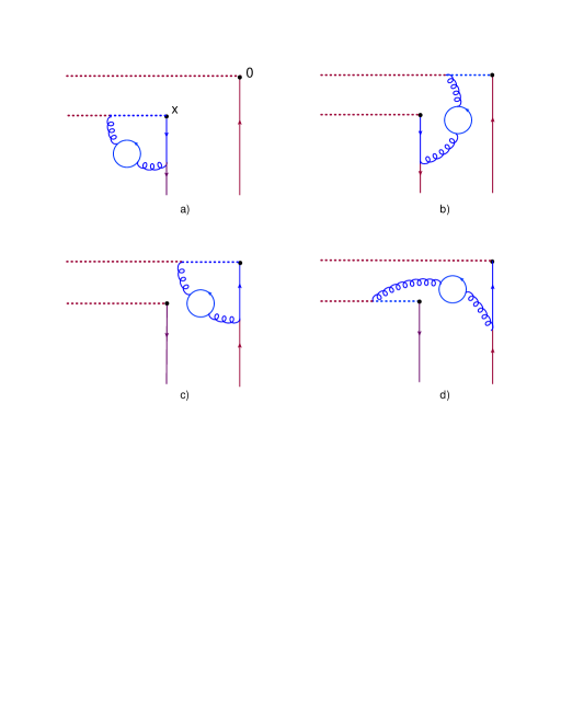
Figure 4: Quark loop correction to quark TMD evolution.

It is convenient to rewrite Eq. (67) as follows

$${\rm RHS~{}of~{}Eq.~{}(\ref{klico1})}~{}=~{}-2i\delta^{-}{d\over d\delta^{-}}\Big{[}\!\int_{-\infty}^{0}\!dz^{+}(z^{+},x_{\perp}|{\ln{\tilde{\mu}^{2}\over-p^{2}}\over p^{2}}\partial^{-}\Psi{1\over p^{2}}|0^{+},-\delta^{-},0_{\perp})~{}-~{}({x_{\perp}\rightarrow 0})\Big{]}$$

$$~{}+2i\delta^{-}{d\over d\delta^{-}}\Big{[}(0^{+},x_{\perp}|{\ln{\tilde{\mu}^{2}\over-p^{2}}\over p^{2}}\Psi{1\over p^{2}}|0^{+},-\delta^{-},0_{\perp})~{}-~{}({x_{\perp}\rightarrow 0})\Big{]}$$ (69)

Since $\partial^{2}\Psi(x^{+})=0$ we can use light-cone expansion (163) from Sec. VII.4. First, note that the second term in the RHS of Eq. (69) can be omitted since the light-cone expansion of the expression in the square brackets depends only on $x_{\perp}^{2}$ and does not depend on $\delta^{-}$. Second, using Eq. (167) for the first line in Eq. (69) we get

$${\rm RHS~{}of~{}Eq.~{}(\ref{klico1})}~{}=~{}\delta^{-}{d\over d\delta^{-}}\Big{[}\!\int_{-\infty}^{0}\!dz^{+}~{}{\Gamma\big{(}{\varepsilon})\over 8\pi^{d\over 2}(x_{\perp}^{2}-2z^{+}\delta^{-})^{\varepsilon}}$$ (70)

$$\times~{}\Big{(}\big{[}\ln{\tilde{\mu}^{2}(x_{\perp}^{2}-2z^{+}\delta^{-})\over 4}+{1\over{\varepsilon}}-\psi(1+{\varepsilon})+\gamma\big{]}\!\int_{0}^{1}\!du~{}\partial^{-}\Psi(uz^{+})+\!\int_{0}^{1}\!du~{}\ln{\bar{u}}~{}\partial^{-}\Psi(uz^{+})\Big{)}~{}-~{}({x_{\perp}\rightarrow 0})\Big{]}$$

Next, using formulas (169) and (170) one obtains

$${\rm RHS~{}of~{}Eq.~{}(\ref{klico1})}~{}=~{}-{1\over 8\pi^{d\over 2}}\!\int_{-\infty}^{0}\!dz^{+}~{}{\Gamma\big{(}{\varepsilon})\over(x_{\perp}^{2}-2z^{+}\delta^{-})^{\varepsilon}}\Big{[}\ln{-\tilde{\mu}^{2}(x_{\perp}^{2}-2z^{+}\delta^{-})\over 4}+{1\over{\varepsilon}}-\psi(1+{\varepsilon})-\psi(1)$$ (71)

$$-\!\int_{0}^{1}{dt\over 1-t}\ln{x_{\perp}^{2}-{2\over t}{x^{\prime}}^{+}\delta^{-}\over x_{\perp}^{2}-2{x^{\prime}}^{+}\delta^{-}}\Big{]}\partial^{-}\Psi(z^{+})~{}-~{}({x_{\perp}\rightarrow 0})$$

$$=~{}{1\over 8\pi^{d\over 2}}\!\int_{-\infty}^{0}\!dz^{+}~{}{\partial\Psi(z^{+})\over\partial z^{+}}\Big{[}{1\over 2}\ln^{2}(x_{\perp}^{2}-2z^{+}\delta^{-})+\ln(x_{\perp}^{2}-2z^{+}\delta^{-})\big{(}\ln{\tilde{\mu}^{2}\over 4}+2\gamma\big{)}-{\rm Li}_{2}\Big{(}{x_{\perp}^{2}\over x_{\perp}^{2}-2z^{+}\delta^{-}}\Big{)}\Big{]}~{}-~{}({x_{\perp}\rightarrow 0})$$

$$=~{}{1\over 16\pi^{d\over 2}}\!\int_{-\infty}^{0}\!dz^{+}~{}{\partial\Psi(z^{+})\over\partial z^{+}}\Big{[}\ln{x_{\perp}^{2}-2z^{+}\delta^{-}\over-2z^{+}\delta^{-}}\Big{(}\ln\tilde{\mu}^{2}{x_{\perp}^{2}-2z^{+}\delta^{-}\over 4}+\ln\tilde{\mu}^{2}{-2z^{+}\delta^{-}\over 4}+4\gamma\Big{)}-2{\rm Li}_{2}\Big{(}{x_{\perp}^{2}\over x_{\perp}^{2}-2z^{+}\delta^{-}}\Big{)}\Big{]}$$

To compare to Eq. (59) we should take $\Psi(z^{+})=\int\!{\textstyle d}\lower 0.12915pt\hbox{\kern-3.80005pt${}^{\scriptstyle-}$}\kern-0.50003pt{}\beta_{B}e^{-i{\varrho}\beta_{B}z^{+}}\Psi(\beta_{B})$. After some algebra we get

$$-i{\varrho}\beta_{B}\!\int_{-\infty}^{0}\!dz^{+}~{}e^{-i{\varrho}\beta_{B}z^{+}}\Big{[}{1\over 2}\ln^{2}(-2z^{+}\delta^{-})+\ln(-2z^{+}\delta^{-})\big{(}\ln{\tilde{\mu}^{2}\over 4}+2\gamma\big{)}\Big{]}$$

$$=~{}-\big{[}\ln{-i\beta_{B}+\epsilon\over 2\delta^{-}}{\varrho}+\gamma\big{]}\big{(}\ln{\tilde{\mu}^{2}\over 4}+2\gamma\big{)}+{1\over 2}[\ln{(-i\beta_{B}+\epsilon){\varrho}\over 2\delta^{-}}+\gamma]^{2}+{\pi^{2}\over 12}$$ (72)

Also,

$$-i{\varrho}\beta_{B}\!\int_{-\infty}^{0}\!dz^{+}~{}e^{-i{\varrho}\beta_{B}z^{+}}\Big{[}{1\over 2}\ln^{2}(x_{\perp}^{2}-2z^{+}\delta^{-})+\ln(x_{\perp}^{2}-2z^{+}\delta^{-})\big{(}\ln{\tilde{\mu}^{2}\over 4}+2\gamma\big{)}-{\rm Li}_{2}\Big{(}{x_{\perp}^{2}\over x_{\perp}^{2}-2z^{+}\delta^{-}}\Big{)}\Big{]}$$

$$=~{}{1\over 2}\ln^{2}x_{\perp}^{2}+\ln x_{\perp}^{2}\big{(}\ln{\tilde{\mu}^{2}\over 4}+2\gamma\big{)}-{\pi^{2}\over 6}~{}+~{}O\big{(}{\delta^{-}\over{\varrho}x_{\perp}^{2}\beta_{B}}\big{)}$$ (73)

where we used the fact that ${2z^{+}\delta^{-}\over x_{\perp}^{2}}\sim{1\over\sigma\beta_{B}s}\sim{m_{\perp}^{2}\over\sigma\beta_{B}s}\ll 1$.

Using these two integrals for Eq. (71) we get

$$\delta^{-}{d\over d\delta^{-}}\langle{\rm T}\{[0^{+},-\infty]_{x}[-\infty,0^{+}]_{0}\Gamma\psi(0^{+},0_{\perp},-\delta^{-})\}\rangle_{\Psi}^{\rm Fig1a-c~{}loop}$$

$$=~{}{b\alpha_{s}^{2}c_{F}\over 16\pi^{2}}\!\int\!{\textstyle d}\lower 0.12915pt\hbox{\kern-3.80005pt${}^{\scriptstyle-}$}\kern-0.50003pt{}\beta_{B}\Psi(\beta_{B})\Big{[}\big{(}\ln{x_{\perp}^{2}{\varrho}\over 2\delta^{-}}[-i\beta_{B}+\epsilon]+\gamma\big{)}\big{(}\ln{x_{\perp}^{2}\tilde{\mu}^{4}\delta^{-}\over 8(-i\beta_{B}+\epsilon){\varrho}}+3\gamma\big{)}-{\pi^{2}\over 2}~{}+~{}O\big{(}{\delta^{-}\over{\varrho}x_{\perp}^{2}\beta_{B}}\big{)}\Big{]}$$ (74)

which agrees with Eq. (59). We will use this method for calculation of quark loops in the gluon case below.

IV Evolution of quark TMDs with gauge links out to $+\infty$

The calculation of diagrams with Wilson lines going to $+\infty$ repeats that the of $-\infty$ case. For the diagrams Fig. 1(a)-1(c) with gauge links out to $+\infty$, instead of Eq. (19), we get

$$\langle[\infty,y^{+}]_{y}\Gamma\psi(y^{+},y_{\perp},\delta^{-})\rangle_{\Psi}^{\rm Fig1c~{}loop}~{}=~{}-ig^{2}c_{F}\!\int\!{\textstyle d}\lower 0.12915pt\hbox{\kern-3.80005pt${}^{\scriptstyle-}$}\kern-0.50003pt{}\beta_{B}{\textstyle d}\lower 0.12915pt\hbox{\kern-3.80005pt${}^{\scriptstyle-}$}\kern-0.50003pt{}p_{B_{\perp}}$$

$$\times~{}e^{-ip_{B}y}\!\int\!{\textstyle d}\lower 0.12915pt\hbox{\kern-3.80005pt${}^{\scriptstyle-}$}\kern-0.50003pt{}\alpha{\textstyle d}\lower 0.12915pt\hbox{\kern-3.80005pt${}^{\scriptstyle-}$}\kern-0.50003pt{}\beta{\textstyle d}\lower 0.12915pt\hbox{\kern-3.80005pt${}^{\scriptstyle-}$}\kern-0.50003pt{}p_{\perp}{1\over\beta-{i\epsilon}}{e^{i\alpha{\varrho}\delta^{-}}\over\alpha\beta s-p_{\perp}^{2}+{i\epsilon}}{s(\beta-\beta_{B})\over\alpha(\beta-\beta_{B})s-(p-p_{B})_{\perp}^{2}+{i\epsilon}}\Gamma\Psi(\beta_{B},p_{B_{\perp}})$$

$$=~{}-g^{2}c_{F}\!\int\!{\textstyle d}\lower 0.12915pt\hbox{\kern-3.80005pt${}^{\scriptstyle-}$}\kern-0.50003pt{}\beta_{B}{\textstyle d}\lower 0.12915pt\hbox{\kern-3.80005pt${}^{\scriptstyle-}$}\kern-0.50003pt{}p_{B_{\perp}}e^{-ip_{B}y}\!\int_{0}^{\infty}\!{\textstyle d}\lower 0.12915pt\hbox{\kern-3.80005pt${}^{\scriptstyle-}$}\kern-0.50003pt{}\alpha\!\int\!{\textstyle d}\lower 0.12915pt\hbox{\kern-3.80005pt${}^{\scriptstyle-}$}\kern-0.50003pt{}p_{\perp}{\beta_{B}se^{i{\alpha\over\sigma}}\over p_{\perp}^{2}[\alpha\beta_{B}s+(p-p_{B})_{\perp}^{2}-{i\epsilon}]}\Gamma\Psi(\beta_{B},p_{B_{\perp}})$$ (75)

and in place of Eq. (14) or Eqs. (21) and (22)

$$\langle[x^{+},\infty]_{x}\Gamma\psi(y^{+},y_{\perp},\delta^{-})\rangle_{\Psi}^{\rm Fig1a,b~{}loop}~{}$$

$$=~{}g^{2}c_{F}\!\int\!{\textstyle d}\lower 0.12915pt\hbox{\kern-3.80005pt${}^{\scriptstyle-}$}\kern-0.50003pt{}\beta_{B}{\textstyle d}\lower 0.12915pt\hbox{\kern-3.80005pt${}^{\scriptstyle-}$}\kern-0.50003pt{}p_{B_{\perp}}e^{-i(p_{B},y)}\!\int\!{\textstyle d}\lower 0.12915pt\hbox{\kern-3.80005pt${}^{\scriptstyle-}$}\kern-0.50003pt{}\alpha{\textstyle d}\lower 0.12915pt\hbox{\kern-3.80005pt${}^{\scriptstyle-}$}\kern-0.50003pt{}\beta{\textstyle d}\lower 0.12915pt\hbox{\kern-3.80005pt${}^{\scriptstyle-}$}\kern-0.50003pt{}p_{\perp}\Big{[}2\pi\delta(\alpha(\beta-\beta_{B})s-(p-p_{B})_{\perp}^{2})(\beta-\beta_{B})s\theta(\alpha){1\over\alpha\beta s-p_{\perp}^{2}-{i\epsilon}}$$

$$\hskip 62.59605pt+~{}{(\beta-\beta_{B})s\over\alpha(\beta-\beta_{B})s-(p-p_{B})_{\perp}^{2}+{i\epsilon}}2\pi\delta(\alpha\beta s-p_{\perp}^{2})\theta(\alpha)\Big{]}{e^{i\alpha{\varrho}\delta^{-}}\over\beta-{i\epsilon}}e^{-i\beta\Delta+i(p,\Delta)_{\perp}}\Gamma\Psi(\beta_{B},p_{B_{\perp}})$$

$$=~{}g^{2}c_{F}\!\int\!{\textstyle d}\lower 0.12915pt\hbox{\kern-3.80005pt${}^{\scriptstyle-}$}\kern-0.50003pt{}\beta_{B}{\textstyle d}\lower 0.12915pt\hbox{\kern-3.80005pt${}^{\scriptstyle-}$}\kern-0.50003pt{}p_{B_{\perp}}\psi(\beta_{B},p_{B_{\perp}})e^{-ip_{B}y}\!\int_{0}^{\infty}\!{\textstyle d}\lower 0.12915pt\hbox{\kern-3.80005pt${}^{\scriptstyle-}$}\kern-0.50003pt{}\alpha~{}e^{i{\alpha\over\sigma}}\!\int\!{\textstyle d}\lower 0.12915pt\hbox{\kern-3.80005pt${}^{\scriptstyle-}$}\kern-0.50003pt{}p_{\perp}~{}\bigg{(}{\beta_{B}s\big{(}e^{-i{p_{\perp}^{2}\over\alpha s}{\varrho}\Delta^{+}+i(p,\Delta)_{\perp}}-1\big{)}\over p_{\perp}^{2}[\alpha\beta_{B}s+(p-p_{B})_{\perp}^{2}-{i\epsilon}]}$$

$$\hskip 125.19212pt+~{}{(p-p_{B})_{\perp}^{2}e^{i(p,\Delta)_{\perp}}\big{[}e^{-i(\beta_{B}+{(p-p_{B})_{\perp}^{2}\over\alpha s}){\varrho}\Delta^{+}}-e^{-i{p_{\perp}^{2}\over\alpha s}{\varrho}\Delta^{+}}\big{]}\over\alpha[\alpha\beta_{B}s+(p-p_{B})_{\perp}^{2}+{i\epsilon}][\alpha\beta_{B}s+(p-p_{B})_{\perp}^{2}-p_{\perp}^{2}]}\bigg{)}\Gamma\Psi(\beta_{B},p_{B_{\perp}})\,.$$ (76)

Note that for gauge links out to $+\infty$ the sign of cutoff $\delta^{-}$ does not matter: the IR cancellation occurs at whatever $\delta$. As discussed above, we choose the sign of splitting in such a way that all relevant distances in the operators are spacelike. With this sign of point splitting in the “$-$” direction we can use the complex conjugate versions of integrals (156)-(161) in the Appendix VII.3.

Similarly, one can easily demonstrate that the contribution of diagrams in Fig.1(d)-1(f) with gauge links out to $+\infty$ differs from Eq. (36) by replacements $\beta_{B}+{i\epsilon}\rightarrow\beta_{B}-{i\epsilon}$ and $\sigma\rightarrow-\sigma$. Repeating the analysis of Sec. II and using (complex conjugate) integral (158) from Appendix VII.3 we get the evolution equation for quark TMDs with gauge links out to $+\infty$ in the form

$$\Big{(}\sigma{d\over d\sigma}+\sigma^{\prime}{d\over d\sigma^{\prime}}\Big{)}{\bar{\psi}}^{\sigma^{\prime}}(\beta^{\prime}_{B},x_{\perp})\Gamma\psi^{\sigma}(\beta_{B},y_{\perp})$$

$$\hskip 5.69054pt=~{}-{g^{2}\over 8\pi^{2}}c_{F}\!\int\!{\textstyle d}\lower 0.12915pt\hbox{\kern-3.80005pt${}^{\scriptstyle-}$}\kern-0.50003pt{}\beta_{B}{\textstyle d}\lower 0.12915pt\hbox{\kern-3.80005pt${}^{\scriptstyle-}$}\kern-0.50003pt{}\beta^{\prime}_{B}{\textstyle d}\lower 0.12915pt\hbox{\kern-3.80005pt${}^{\scriptstyle-}$}\kern-0.50003pt{}p_{B_{\perp}}{\textstyle d}\lower 0.12915pt\hbox{\kern-3.80005pt${}^{\scriptstyle-}$}\kern-0.50003pt{}p^{\prime}_{B_{\perp}}{\bar{\psi}}^{\sigma^{\prime}}(\beta^{\prime}_{B},x_{\perp})\Gamma\psi^{\sigma}(\beta_{B},y_{\perp})e^{-i\beta^{\prime}_{B}{\varrho}x^{+}-i\beta_{B}{\varrho}y^{+}}$$

$$\hskip 5.69054pt\times~{}\Big{[}\ln\Big{(}{i\over 4}(\beta_{B}-{i\epsilon})\sigma sb_{\perp}^{2}e^{\gamma}\Big{)}+\ln\Big{(}{i\over 4}(\beta^{\prime}_{B}-{i\epsilon})\sigma^{\prime}sb_{\perp}^{2}e^{\gamma}\Big{)}\Big{]}~{}+~{}O\Big{(}{m_{\perp}^{2}\over\beta_{B}\sigma s},{m_{\perp}^{2}\over\beta^{\prime}_{B}\sigma^{\prime}s}\Big{)}$$ (77)

and the solution is

$${\bar{\psi}}^{\sigma^{\prime}}(\beta^{\prime}_{B},x_{\perp})\Gamma\psi^{\sigma}(\beta_{B},y_{\perp})$$ (78)

$$=~{}e^{-{\alpha_{s}c_{F}\over 4\pi}\ln{\sigma^{\prime}\over\sigma^{\prime}_{0}}\big{[}\ln{\sigma^{\prime}\sigma^{\prime}_{0}}+2\ln\big{(}{i\over 4}(\beta^{\prime}_{B}-{i\epsilon})sb_{\perp}^{2}e^{\gamma}\big{)}\big{]}}{\bar{\psi}}^{\sigma^{\prime}_{0}}(\beta^{\prime}_{B},x_{\perp})\Gamma\psi^{\sigma_{0}}(\beta_{B},y_{\perp})e^{-{\alpha_{s}c_{F}\over 4\pi}\ln{\sigma\over\sigma_{0}}\big{[}\ln{\sigma\sigma_{0}}+2\ln\big{(}{i\over 4}(\beta^{\prime}_{B}-{i\epsilon})sb_{\perp}^{2}e^{\gamma}\big{)}\big{]}}$$

where ${\bar{\psi}}^{\sigma^{\prime}}(\beta^{\prime}_{B},x_{\perp})$ and $\psi^{\sigma}(\beta_{B},y_{\perp})$ are given by formulas (26) with gauge links out to $+\infty$:

$${\bar{\psi}}^{\sigma}(x^{+},x_{\perp})~{}\equiv~{}{\bar{\psi}}\big{(}x^{+},x_{\perp},-{1\over\rho\sigma}\big{)}[x^{+},-\infty]_{x},~{}~{}~{}~{}\psi^{\sigma}(y^{+},y_{\perp})~{}\equiv~{}[-\infty,y^{+}]_{y}\psi\big{(}y^{+},y_{\perp},-{1\over\rho\sigma}\big{)},$$ (79)

In the coordinate space Eq. (78) corresponds to

$${\bar{\psi}}^{\sigma^{\prime}}(x^{+},x_{\perp})\Gamma\psi^{\sigma}(y^{+},y_{\perp})~{}=~{}{1\over 4\pi^{2}}e^{-{\alpha_{s}c_{F}\over 4\pi}\big{(}\ln{\sigma^{\prime}\over\sigma^{\prime}_{0}}\ln{\sigma^{\prime}\sigma^{\prime}_{0}}+\ln{\sigma\over\sigma_{0}}\ln{\sigma\sigma_{0}}\big{)}}$$ (80)

$$\times~{}\int\!dz^{+}\bigg{[}{i\Gamma\big{(}1-{\alpha_{s}c_{F}\over 2\pi}\ln{\sigma^{\prime}\over\sigma^{\prime}_{0}}\big{)}\over(x^{+}-z^{+}+{i\epsilon})^{1-{\alpha_{s}c_{F}\over 2\pi}\ln{\sigma^{\prime}\over\sigma^{\prime}_{0}}}}+{\rm c.c.}\bigg{]}\int\!dw^{+}\bigg{[}{i\Gamma\big{(}1-{\alpha_{s}c_{F}\over 2\pi}\ln{\sigma\over\sigma_{0}}\big{)}\over(y^{+}-w^{+}+{i\epsilon})^{1-{\alpha_{s}c_{F}\over 2\pi}\ln{\sigma\over\sigma_{0}}}}+{\rm c.c.}\bigg{]}{\bar{\psi}}^{\sigma^{\prime}_{0}}(x^{+},x_{\perp})\Gamma\psi^{\sigma_{0}}(y^{+},y_{\perp})$$

Now we have $z^{+}\geq x^{+}$ and $w^{+}\geq y^{+}$ so the evolution goes out to $+\infty$.

For completeness, let us present the final result for the evolution with running coupling which is obtained from Eq. (65) by replacement $-i\tau_{B}+\epsilon$ to $i\tau_{B}+\epsilon$

$${\bar{\psi}}^{\sigma}(\beta^{\prime}_{B},x_{\perp})\Gamma\psi^{\sigma}(\beta_{B},y_{\perp})~{}=~{}e^{-{2c_{F}\over\pi b_{0}^{2}}\big{[}\big{(}{1\over\alpha_{s}(\tilde{b}_{\perp}^{-1})}-{b_{0}\over 2}\ln[i(\tau^{\prime}_{B}-{i\epsilon})]\big{)}\ln{\alpha_{s}(\mu_{\sigma^{\prime}})\over\alpha_{s}(\mu_{\sigma^{\prime}_{0}})}+{1\over\alpha_{s}(\mu_{\sigma^{\prime}})}-{1\over\alpha_{s}(\mu_{\sigma^{\prime}_{0}})}\big{]}}$$

$$\times~{}e^{-{2c_{F}\over\pi b_{0}^{2}}\big{[}\big{(}{1\over\alpha_{s}(\tilde{b}_{\perp}^{-1})}-{b_{0}\over 2}\ln[i(\tau_{B}-{i\epsilon})]\big{)}\ln{\alpha_{s}(\mu_{\sigma})\over\alpha_{s}(\mu_{\sigma_{0}})}+{1\over\alpha_{s}(\mu_{\sigma})}-{1\over\alpha_{s}(\mu_{\sigma_{0}})}\big{]}}{\bar{\psi}}^{\sigma_{0}}(\beta^{\prime}_{B},x_{\perp})\Gamma\psi^{\sigma_{0}}(\beta_{B},y_{\perp})$$ (81)

V Rapidity evolution of gluon TMDs

V.1 Leading-order contribution

The gluon TMD is defined by the operator (5)

$$F^{-i}(x^{+},x_{\perp})[x,x\pm\infty n]~{}[x_{\perp},y_{\perp}]_{\pm\infty n}[\pm\infty n+y,y]F^{-j}(y^{+},y_{\perp})$$ (82)

The typical process determined by gluon TMD (with gauge links out to $-\infty$) is Higgs production by gluon-gluon fusion in the Sudakov region. If one approximates $t$-quark loop by a point vertex, the differential cross section is determined by the “hadronic tensor” given by the formula similar to Eq. (1) with gluon TMDs Mulders:2000sh

$$G(x_{B},z_{\perp},\eta)~{}=~{}{-x_{B}^{-1}\over 2\pi p^{-}}\!\int\!dz^{+}~{}e^{-ix_{B}p^{-}z^{+}}\langle P|F^{-i,a}(z^{+},z_{\perp})([z,z\pm\infty n]~{}[z_{\perp},0_{\perp}]_{\pm\infty n}[\pm\infty n,0])^{ab}F^{-,b}_{~{}~{}i}(0)|P\rangle$$ (83)

in place of quark ones (see the discussion in Ref. Balitsky:2017flc ).

The leading-order rapidity evolution was found in Ref. Balitsky:2019ayf . Here we first repeat the LO derivation and then obtain the running-coupling correction by the BLM prescription. Similar to the quark case, we define rapidity-regularized operators by

$$\tilde{\mathscr{F}}^{\sigma,a}_{i}(x_{\perp},x^{+})~{}=~{}(F^{-}_{~{}~{}i})^{b}(x^{+},x_{\perp},-\delta^{-})[x^{+},-\infty]_{x}^{ba},~{}~{}~{}~{}~{}\mathscr{F}^{\sigma,a}_{i}(y_{\perp},y^{+})~{}=~{}[-\infty,y^{+}]_{y}^{ab}(F^{-}_{~{}~{}i})^{b}(x^{+},x_{\perp},-\delta^{\prime-})$$ (84)

where $\delta^{-}={1\over{\varrho}\sigma}$. Let us emphasize again that we use the point-splitting operators in the RHSs only for the perturbative calculations.

Similar to the quark case considered above, to find the LO evolution equation we calculate diagrams in the background field $A^{\rm ext}_{\mu}(x_{+},x_{\perp})$ and use point splitting for regularization of rapidity divergences,

$$\Big{(}\sigma{d\over d\sigma}+\sigma^{\prime}{d\over d\sigma^{\prime}}\Big{)}\langle F^{-i,a}(x^{+},x_{\perp},-\delta^{\prime-})[x^{+},-\infty]_{x}^{ab}~{}[x_{\perp},y_{\perp}]_{-\infty^{+}}^{bc}[-\infty,y^{+}]_{y}^{cd}F^{-,d}_{~{}~{}i}(y^{+},y_{\perp},-\delta^{-})\rangle_{\cal A}\,.$$ (85)

Also, we use the $A^{-}_{\rm ext}=0$ gauge for the background field and background-Feynman (bF) gauge for quantum gluons. As we mentioned above, in such a gauge the contribution of gauge link $[x_{\perp},y_{\perp}]_{-\infty^{+}}$ can be neglected. Moreover, in the bF gauge the product $gA^{\rm ext}_{\mu}$ is renorm invariant so there is no need to consider self-energy diagrams, and the one-loop evolution of the operator (5) looks the same as in Fig. 1 but with gluons instead of quarks. We will also use the notation ${\cal A}_{\mu}\equiv gA^{\rm ext}_{\mu}$ and ${\cal F}_{\mu\nu}=\partial_{\mu}{\cal A}_{\nu}-\partial_{\nu}{\cal A}_{\mu}-i[{\cal A}_{\mu},{\cal A}_{\nu}]$.

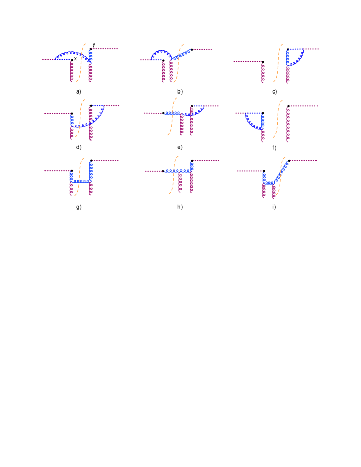
Figure 5: One-loop diagrams for gluon TMD operator (5) in the background gluon field.

Gluon propagators in the bF gauge are

$$\langle{\rm T}\{A^{a}_{\mu}(x)A^{b}_{\nu}(y)\}\rangle~{}=~{}(x|{-i\over{\cal P}^{2}g_{\mu\nu}+2i{\cal F}_{\mu\nu}+{i\epsilon}}|y)^{ab}~{}=~{}(x|{-ig_{\mu\nu}g^{ab}\over p^{2}+{i\epsilon}}|y)-2(x|{1\over p^{2}+{i\epsilon}}{\cal F}^{ab}_{\mu\nu}{1\over p^{2}+{i\epsilon}}|y)~{}+~{}O({\cal F}^{2})$$

$$\langle\tilde{\rm T}\{A^{a}_{\mu}(x)A^{b}_{\nu}(y)\}\rangle~{}=~{}(x|{i\over{\cal P}^{2}g_{\mu\nu}+2i{\cal F}_{\mu\nu}-{i\epsilon}}|y)^{ab}~{}=~{}(x|{ig_{\mu\nu}g^{ab}\over p^{2}-{i\epsilon}}|y)+2(x|{1\over p^{2}-{i\epsilon}}{\cal F}^{ab}_{\mu\nu}{1\over p^{2}-{i\epsilon}}|y)~{}+~{}O({\cal F}^{2})$$

$$\langle A^{a}_{\mu}(x)A^{b}_{\nu}(y)\rangle~{}=~{}-(x|{1\over{\cal P}^{2}g_{\mu\xi}+2i{\cal F}_{\mu\xi}-{i\epsilon}}p^{2}{\textstyle\delta}\lower 0.12915pt\hbox{\kern-3.80005pt${}^{\scriptstyle-}$}\kern-0.50003pt{}(p^{2})\theta(p_{0})p^{2}{1\over{\cal P}^{2}g_{\xi\nu}+2i{\cal F}_{\xi\nu}+{i\epsilon}}|y)^{ab}$$ (86)

$$=~{}-g_{\mu\nu}g^{ab}(x|2\pi\delta(p^{2})\theta(p_{0})|y)+4\pi i(x|{1\over p^{2}-{i\epsilon}}\big{[}{\cal F}_{\mu\nu}^{ab}\delta(p^{2})\theta(p_{0})+\delta(p^{2})\theta(p_{0}){\cal F}^{ab}_{\mu\nu}\big{]}{1\over p^{2}+{i\epsilon}}|y)~{}+~{}O({\cal F}^{2})$$

Here $a$ and $b$ are adjoint indices and

$$(x|f(p)|y)=\int\!{\textstyle d}\lower 0.12915pt\hbox{\kern-3.80005pt${}^{\scriptstyle-}$}\kern-0.50003pt{}p~{}e^{-p(x-y)}f(p),~{}~{}~{}~{}~{}(x|f({\cal A})|y)=f({\cal A}(x))\delta(x-y)$$

are Schwinger’s notations for propagators in background fields.

Let us start with diagrams in Fig. 5(a)-5(c). The contribution of the virtual diagram in Fig. 5(c) is

$$\langle\mathscr{F}^{\sigma,a}(y^{+},y_{\perp})\rangle_{\cal A}^{\rm Fig.~{}\ref{fig:gldiagrams}c}~{}=~{}-ig^{2}\!\int_{-\infty}^{y^{+}}\!dy^{\prime+}\langle A^{-,ab}(y^{\prime+},y_{\perp})(D^{-}A^{j,b}-D^{j}A^{-,b})(y^{+},y_{\perp},-\delta^{-})\rangle_{\cal A}$$ (87)

$$=~{}-2g^{2}N_{c}\!\int_{-\infty}^{y^{+}}\!\!dy^{\prime+}{\varrho}~{}(y^{\prime+},y_{\perp}|{1\over p^{2}+{i\epsilon}}{\cal F}^{-j,a}{1\over p^{2}+{i\epsilon}}p^{-}|y^{+},y_{\perp},-\delta^{-})$$

$$=-2ig^{2}N_{c}(y|{1\over\beta+{i\epsilon}}{1\over p^{2}+{i\epsilon}}{\cal F}^{-j,a}{\beta\over p^{2}+{i\epsilon}}|y-\delta^{-})$$

$$=~{}-isg^{2}N_{c}\!\int\!{\textstyle d}\lower 0.12915pt\hbox{\kern-3.80005pt${}^{\scriptstyle-}$}\kern-0.50003pt{}\beta_{B}{\textstyle d}\lower 0.12915pt\hbox{\kern-3.80005pt${}^{\scriptstyle-}$}\kern-0.50003pt{}p_{B_{\perp}}{\cal F}^{-j,a}(\beta_{B},p_{B_{\perp}})e^{-ip_{B}y}\!\int\!{\textstyle d}\lower 0.12915pt\hbox{\kern-3.80005pt${}^{\scriptstyle-}$}\kern-0.50003pt{}\alpha{{\textstyle d}\lower 0.12915pt\hbox{\kern-3.80005pt${}^{\scriptstyle-}$}\kern-0.50003pt{}\beta\over\beta+{i\epsilon}}~{}\!\int\!{\textstyle d}\lower 0.12915pt\hbox{\kern-3.80005pt${}^{\scriptstyle-}$}\kern-0.50003pt{}p_{\perp}{(\beta-\beta_{B})e^{-i\alpha{\varrho}\delta^{-}}\over(\alpha\beta s-p_{\perp}^{2}+{i\epsilon})(\alpha(\beta-\beta_{B})s-(p-p_{B})_{\perp}^{2}+{i\epsilon})}$$

where ${\cal F}^{-i}(\beta_{B},p_{B_{\perp}})$ is the Fourier transform of the background field:

$${\cal F}^{-i}(\beta_{B},p_{B_{\perp}})~{}=~{}\!\int\!dz^{+}dz_{\perp}~{}{\cal F}^{-i}(z^{+},z_{\perp})~{}e^{i\beta_{B}{\varrho}z^{+}-i(p_{B},z)_{\perp}}.~{}~{}~{}~{}~{}~{}~{}$$ (88)

It is worth noting that similar to the quark case, in a general gauge one should replace background fields by

$${\cal F}^{a}_{-i}(z^{+},z_{\perp})~{}\rightarrow~{}[z^{+},\pm\infty^{+}]^{ab}{\cal F}^{b}_{-i}(z^{+},z_{\perp})$$ (89)

where the direction of Wilson lines corresponds to the choice of $\pm\infty$ in Eq. (82).

The integral over momenta in Eq. (87) is the same as in Eq. (19) so we get

$$\langle\mathscr{F}^{\sigma,a}_{j}(y_{\perp},y^{\perp})\rangle^{\rm Fig.~{}\ref{fig:gldiagrams}c}_{\cal A}~{}=~{}-ig^{2}\!\int_{-\infty}^{y^{+}}\!dy^{\prime+}~{}A^{-,ab}(y^{\prime+},y_{\perp},-\delta^{-})(D^{-}A^{j,b}-D^{j}A^{-,b})(y^{+},y_{\perp},-\delta^{-})$$ (90)

$$=~{}-g^{2}N_{c}\!\int\!{\textstyle d}\lower 0.12915pt\hbox{\kern-3.80005pt${}^{\scriptstyle-}$}\kern-0.50003pt{}\beta_{B}{\textstyle d}\lower 0.12915pt\hbox{\kern-3.80005pt${}^{\scriptstyle-}$}\kern-0.50003pt{}p_{B_{\perp}}e^{-ip_{B}y}{\cal F}^{-j,a}(\beta_{B},p_{B_{\perp}})\!\int_{0}^{\infty}\!{\textstyle d}\lower 0.12915pt\hbox{\kern-3.80005pt${}^{\scriptstyle-}$}\kern-0.50003pt{}\alpha\!\int\!{\textstyle d}\lower 0.12915pt\hbox{\kern-3.80005pt${}^{\scriptstyle-}$}\kern-0.50003pt{}p_{\perp}{\beta_{B}s\over p_{\perp}^{2}[\alpha\beta_{B}s+(p-p_{B})_{\perp}^{2}+{i\epsilon}]}e^{-i{\alpha\over\sigma}}$$ (91)

Next, consider diagrams in Fig. 5(a) and 5(b)

$$\langle[x^{+},-\infty]_{x}^{ba}F^{-j,a}(y^{+},y_{\perp},-\delta^{-})\rangle_{\cal A}^{\rm Fig.~{}\ref{fig:gldiagrams}a,b}~{}=~{}ig^{2}\!\int_{-\infty}^{x^{+}}\!dx^{\prime+}~{}A^{-,ba}(x^{\prime+},x_{\perp})(D^{-}A^{j,a}-D^{j}A^{-,a})(y^{+},y_{\perp},-\delta^{-})$$

$$=~{}-2ig^{2}N_{c}\!\int_{-\infty}^{x^{+}}\!\!dx^{\prime+}(x^{\prime}|\big{(}{1\over p^{2}-{i\epsilon}}{\cal F}^{-j,b}2\pi\delta(p^{2})\theta(p_{0})+2\pi\delta(p^{2})\theta(p_{0}){\cal F}^{-j,b}{1\over p^{2}+{i\epsilon}}\big{)}p^{-}|y)$$

$$=~{}2g^{2}N_{c}(x|{1\over\beta+{i\epsilon}}\big{(}{1\over p^{2}-{i\epsilon}}{\cal F}^{-j,b}{\textstyle\delta}\lower 0.12915pt\hbox{\kern-3.80005pt${}^{\scriptstyle-}$}\kern-0.50003pt{}(p^{2})\theta(p_{0})\beta+{\textstyle\delta}\lower 0.12915pt\hbox{\kern-3.80005pt${}^{\scriptstyle-}$}\kern-0.50003pt{}(p^{2})\theta(p_{0}){\cal F}^{-j,b}{\beta\over p^{2}+{i\epsilon}}\big{)}|y)$$

$$=~{}sg^{2}N_{c}\!\!\int\!\!{\textstyle d}\lower 0.12915pt\hbox{\kern-3.80005pt${}^{\scriptstyle-}$}\kern-0.50003pt{}\beta_{B}{\textstyle d}\lower 0.12915pt\hbox{\kern-3.80005pt${}^{\scriptstyle-}$}\kern-0.50003pt{}p_{B_{\perp}}{\cal F}^{-j,b}(\beta_{B},p_{B_{\perp}}\!)e^{-ip_{B}y}\!\!\int\!\!{\textstyle d}\lower 0.12915pt\hbox{\kern-3.80005pt${}^{\scriptstyle-}$}\kern-0.50003pt{}\alpha{{\textstyle d}\lower 0.12915pt\hbox{\kern-3.80005pt${}^{\scriptstyle-}$}\kern-0.50003pt{}\beta\over\beta+{i\epsilon}}~{}e^{-i\beta{\varrho}\Delta^{+}}$$

$$\times~{}\int\!{\textstyle d}\lower 0.12915pt\hbox{\kern-3.80005pt${}^{\scriptstyle-}$}\kern-0.50003pt{}p_{\perp}~{}e^{i(p,\Delta)_{\perp}}\Big{[}{(\beta-\beta_{B})\theta(\alpha)\over\alpha\beta s-p_{\perp}^{2}-{i\epsilon}}2\pi\delta[(\beta-\beta_{B})\alpha s-(p-p_{B})_{\perp}^{2}]+{(\beta-\beta_{B})\theta(\alpha)2\pi\delta(\alpha\beta s-p_{\perp}^{2})\over\alpha(\beta-\beta_{B})s-(p-p_{B})_{\perp}^{2}+{i\epsilon}}\Big{]}$$ (92)

The integral over momenta is the same as in the quark case [see Eq. (14)] so similar to Eqs. (21) and (22) we get

$$\langle[x^{+},-\infty]_{x}^{ba}F^{-j,a}(y^{+},y_{\perp},-\delta^{-})\rangle_{\cal A}$$

$$=~{}g^{2}N_{c}\!\!\int\!\!{\textstyle d}\lower 0.12915pt\hbox{\kern-3.80005pt${}^{\scriptstyle-}$}\kern-0.50003pt{}\beta_{B}{\textstyle d}\lower 0.12915pt\hbox{\kern-3.80005pt${}^{\scriptstyle-}$}\kern-0.50003pt{}p_{B_{\perp}}{\cal F}^{-j,b}(\beta_{B},p_{B_{\perp}}\!)e^{-ip_{B}y}\!\int_{0}^{\infty}\!{\textstyle d}\lower 0.12915pt\hbox{\kern-3.80005pt${}^{\scriptstyle-}$}\kern-0.50003pt{}\alpha\!\int\!{\textstyle d}\lower 0.12915pt\hbox{\kern-3.80005pt${}^{\scriptstyle-}$}\kern-0.50003pt{}p_{\perp}\Big{\{}{\beta_{B}se^{-i{p_{\perp}^{2}\over\alpha s}{\varrho}\Delta^{+}+i(p,\Delta)}\over p_{\perp}^{2}[\alpha\beta_{B}s+(p-p_{B})_{\perp}^{2}+{i\epsilon}[}e^{-i{\alpha\over\sigma}}$$

$$+~{}{(p-p_{B})_{\perp}^{2}e^{i(p,\Delta)_{\perp}}\big{[}e^{-i(\beta_{B}+{(p-p_{B})_{\perp}^{2}\over\alpha s}){\varrho}\Delta^{+}}-e^{-i{p_{\perp}^{2}\over\alpha s}{\varrho}\Delta^{+}}\big{]}\over[\alpha\beta_{B}s+(p-p_{B})_{\perp}^{2}+{i\epsilon}][\alpha\beta_{B}s+(p-p_{B})_{\perp}^{2}-p_{\perp}^{2}]}e^{-i{\alpha\over\sigma}}\Big{\}}$$ (93)

and therefore

$$\langle[x^{+},-\infty]_{x}^{ab}[-\infty,y^{+}]_{y}^{bc}F^{-j,c}(y^{+},y_{\perp},-\delta^{-})\rangle_{\cal A}^{\rm Fig.~{}\ref{fig:gldiagrams}a-c}$$ (94)

$$\hskip 62.59605pt=~{}g^{2}N_{c}\!\!\int\!\!{\textstyle d}\lower 0.12915pt\hbox{\kern-3.80005pt${}^{\scriptstyle-}$}\kern-0.50003pt{}\beta_{B}{\textstyle d}\lower 0.12915pt\hbox{\kern-3.80005pt${}^{\scriptstyle-}$}\kern-0.50003pt{}p_{B_{\perp}}{\cal F}^{-j,b}(\beta_{B},p_{B_{\perp}}\!)e^{-ip_{B}y}\!\int_{0}^{\infty}\!{\textstyle d}\lower 0.12915pt\hbox{\kern-3.80005pt${}^{\scriptstyle-}$}\kern-0.50003pt{}\alpha~{}e^{-i{\alpha\over\sigma}}\!\int\!{\textstyle d}\lower 0.12915pt\hbox{\kern-3.80005pt${}^{\scriptstyle-}$}\kern-0.50003pt{}p_{\perp}~{}\bigg{(}{\beta_{B}s\big{(}e^{-i{p_{\perp}^{2}\over\alpha s}{\varrho}\Delta^{+}+i(p,\Delta)_{\perp}}-1\big{)}\over p_{\perp}^{2}[\alpha\beta_{B}s+(p-p_{B})_{\perp}^{2}+{i\epsilon}]}$$

$$\hskip 125.19212pt+~{}{(p-p_{B})_{\perp}^{2}e^{i(p,\Delta)_{\perp}}\big{[}e^{-i(\beta_{B}+{(p-p_{B})_{\perp}^{2}\over\alpha s}){\varrho}\Delta^{+}}-e^{-i{p_{\perp}^{2}\over\alpha s}{\varrho}\Delta^{+}}\big{]}\over\alpha[\alpha\beta_{B}s+(p-p_{B})_{\perp}^{2}+{i\epsilon}][\alpha\beta_{B}s+(p-p_{B})_{\perp}^{2}-p_{\perp}^{2}]}\bigg{)}$$

The integral is the same as in Eq. (23) for the quark case, so similar to Eq. (31) we get the contribution of diagrams in Fig. 5(a)-5(c) in the form

$$\sigma{d\over d\sigma}\langle[x^{+},-\infty]_{x}^{ab}[-\infty,y^{+}]_{y}^{bc}gF^{-j,c}\big{(}y^{+},y_{\perp},-{1\over{\varrho}\sigma}\big{)}\rangle_{\cal A}^{\rm Fig.~{}\ref{fig:gldiagrams}a-c}$$

$$\hskip 5.69054pt=~{}-{g^{2}\over 8\pi^{2}}N_{c}\!\int\!{\textstyle d}\lower 0.12915pt\hbox{\kern-3.80005pt${}^{\scriptstyle-}$}\kern-0.50003pt{}\beta_{B}~{}{\cal F}^{-j,b}(\beta_{B},y_{\perp})e^{-i\beta_{B}{\varrho}y^{+}}\ln\Big{(}-{i\over 4}(\beta_{B}+{i\epsilon})\sigma s\Delta_{\perp}^{2}e^{\gamma}\Big{)}~{}+~{}O\big{(}{m_{\perp}^{2}\over\beta_{B}\sigma s}\big{)}$$ (96)

where

$${\cal F}^{-i}(\beta_{B},z_{\perp})~{}=~{}\!\int\!dz^{+}~{}{\cal F}^{-i}(z^{+},z_{\perp})e^{i\beta_{B}{\varrho}z^{+}}~{}~{}~{}~{}~{}~{}~{}$$ (97)

in accordance with Eq. (88).

A similar calculation of diagrams in Fig. 5(d)-5(f) yields

$$\langle F^{-i,a}(x^{+},x_{\perp},-\delta^{\prime-})[x^{+},-\infty]_{x}^{ab}[-\infty,y^{+}]_{y}^{bc}\rangle_{\cal A}$$

$$=~{}\langle(D^{-}A^{i,a}-D^{i}A^{-,a})(x^{+},x_{\perp},-\delta^{\prime-})ig^{2}\bigg{[}\!\int_{-\infty}^{x^{+}}\!dx^{\prime+}A^{-,ac}(x^{+},x_{\perp})-\!\int_{-\infty}^{y^{+}}\!dy^{\prime+}A^{-,ac}(y^{+},y_{\perp})\bigg{]}\rangle_{\cal A}$$ (98)

$$\hskip 31.29802pt=~{}g^{2}N_{c}\!\int\!{\textstyle d}\lower 0.12915pt\hbox{\kern-3.80005pt${}^{\scriptstyle-}$}\kern-0.50003pt{}\beta_{B}{\textstyle d}\lower 0.12915pt\hbox{\kern-3.80005pt${}^{\scriptstyle-}$}\kern-0.50003pt{}p_{B_{\perp}}e^{-ip_{B}x}g{\cal F}^{-i,c}(\beta_{B},p_{B_{\perp}})\!\int\!{\textstyle d}\lower 0.12915pt\hbox{\kern-3.80005pt${}^{\scriptstyle-}$}\kern-0.50003pt{}p_{\perp}\!\int_{0}^{\infty}\!{\textstyle d}\lower 0.12915pt\hbox{\kern-3.80005pt${}^{\scriptstyle-}$}\kern-0.50003pt{}\alpha~{}e^{i{\alpha\over\sigma^{\prime}}}\bigg{(}{\beta_{B}s\big{(}e^{i(p,\Delta)_{\perp}-i{p_{\perp}^{2}\over\alpha s}{\varrho}\Delta^{+}}-1\big{)}\over\alpha\beta_{B}s-(p+p_{B})_{\perp}^{2}+{i\epsilon}}$$

$$\hskip 62.59605pt+~{}{(p+p_{B})_{\perp}^{2}\big{[}e^{i(p,\Delta)_{\perp}}e^{-i{(p+p_{B})_{\perp}^{2}\over\alpha s}{\varrho}\Delta^{+}+i\beta_{B}{\varrho}\Delta^{+}}-e^{-i{p_{\perp}^{2}\over\alpha s}{\varrho}\Delta^{+}}\big{]}\over\alpha[\alpha\beta_{B}s+p_{\perp}^{2}-(p+p_{B})_{\perp}^{2}+{i\epsilon}][\alpha\beta_{B}s-(p+p_{B})_{\perp}^{2}+{i\epsilon}]}\bigg{)}$$ (99)

and therefore [see Eq. (36)] we get

$$\sigma^{\prime}{d\over d\sigma^{\prime}}\langle gF^{-i,a}\big{(}x^{+},x_{\perp},-{1\over{\varrho}\sigma^{\prime}}\big{)}[x^{+},-\infty]_{x}[-\infty,y^{+}]_{y}\rangle_{\Psi}^{\rm Fig.~{}\ref{fig:gldiagrams}d-f}$$

$$\hskip 5.69054pt=~{}-{g^{2}\over 8\pi^{2}}N_{c}\!\int\!{\textstyle d}\lower 0.12915pt\hbox{\kern-3.80005pt${}^{\scriptstyle-}$}\kern-0.50003pt{}\beta_{B}{\cal F}^{-i,c}(\beta_{B},x_{\perp})e^{-i\beta_{B}{\varrho}x^{+}}\ln\Big{(}-{i\over 4}(\beta_{B}+{i\epsilon})\sigma^{\prime}s\Delta_{\perp}^{2}e^{\gamma}\Big{)}~{}+~{}O\big{(}{m_{\perp}^{2}\over\beta_{B}\sigma^{\prime}s}\big{)}$$ (100)

Finally, let us discuss “handbag” diagrams in Figs. 5(g)-5(i). Similar to the quark case, since the separation between $x$ and $y$ is spacelike we can replace the product of operators in Eq. (85) by the T-product and get

$$\langle{\rm T}\{F^{-i,a}(x^{+},x_{\perp},-\delta^{\prime-})F^{-,a}_{~{}~{}i}(y^{+},y_{\perp},-\delta^{-})\}\rangle_{\cal A}~{}=-i(x|({\cal P}^{-}\delta^{i}_{\xi}-{\cal P}^{i}\delta^{-}_{\xi}){1\over{\cal P}^{2}g_{\xi\eta}+2ig{\cal F}_{\xi\eta}+{i\epsilon}}({\cal P}^{-}g_{i\eta}-{\cal P}_{i}\delta^{-}_{\eta})|y)^{aa}_{\rm Fig.\ref{fig:gldiagrams}g-i}$$

$$=~{}2g^{2}(x|{\cal P}^{i}{1\over{\cal P}^{2}+{i\epsilon}}{\cal F}^{-i}{1\over{\cal P}^{2}+{i\epsilon}}{\cal F}^{-}_{~{}~{}i}{1\over{\cal P}^{2}+{i\epsilon}}|y)^{aa}=~{}-4g^{2}N_{c}\!\int\!{\textstyle d}\lower 0.12915pt\hbox{\kern-3.80005pt${}^{\scriptstyle-}$}\kern-0.50003pt{}\beta_{B}{\textstyle d}\lower 0.12915pt\hbox{\kern-3.80005pt${}^{\scriptstyle-}$}\kern-0.50003pt{}p_{B_{\perp}}{\textstyle d}\lower 0.12915pt\hbox{\kern-3.80005pt${}^{\scriptstyle-}$}\kern-0.50003pt{}\beta^{\prime}_{B}{\textstyle d}\lower 0.12915pt\hbox{\kern-3.80005pt${}^{\scriptstyle-}$}\kern-0.50003pt{}{p^{\prime}}_{B_{\perp}}e^{-ip^{\prime}_{B}x-ip_{B}y}{\cal F}^{-i,a}(\beta^{\prime}_{B},p^{\prime}_{B_{\perp}})$$

$$\times~{}{\cal F}^{-,a}_{~{}~{}i}(\beta_{B},p_{B_{\perp}})(x|{(p+p^{\prime}_{B})^{i}\over(p+p_{B})^{2}+{i\epsilon}}{1\over p^{2}+{i\epsilon}}{(p-p_{B})_{i}\over(p-p_{B})^{2}+{i\epsilon}}|y)$$

$$=~{}-2sg^{2}N_{c}\!\int\!{\textstyle d}\lower 0.12915pt\hbox{\kern-3.80005pt${}^{\scriptstyle-}$}\kern-0.50003pt{}\beta_{B}{\textstyle d}\lower 0.12915pt\hbox{\kern-3.80005pt${}^{\scriptstyle-}$}\kern-0.50003pt{}p_{B_{\perp}}{\textstyle d}\lower 0.12915pt\hbox{\kern-3.80005pt${}^{\scriptstyle-}$}\kern-0.50003pt{}\beta^{\prime}_{B}{\textstyle d}\lower 0.12915pt\hbox{\kern-3.80005pt${}^{\scriptstyle-}$}\kern-0.50003pt{}{p^{\prime}}_{B_{\perp}}e^{-ip^{\prime}_{B}x-ip_{B}y}{\cal F}^{-i,a}(\beta^{\prime}_{B},p^{\prime}_{B_{\perp}}){\cal F}^{-,a}_{~{}~{}i}(\beta_{B},p_{B_{\perp}})$$

$$\times~{}\!\int\!{\textstyle d}\lower 0.12915pt\hbox{\kern-3.80005pt${}^{\scriptstyle-}$}\kern-0.50003pt{}\alpha{\textstyle d}\lower 0.12915pt\hbox{\kern-3.80005pt${}^{\scriptstyle-}$}\kern-0.50003pt{}\beta{\textstyle d}\lower 0.12915pt\hbox{\kern-3.80005pt${}^{\scriptstyle-}$}\kern-0.50003pt{}p_{\perp}~{}e^{i\alpha{\varrho}(\delta^{\prime}-\delta)^{-}+i\beta{\varrho}\Delta^{+}}{e^{-i(p,\Delta)_{\perp}}(p+p^{\prime}_{B})^{i}(p-p_{B})_{i}\over(\alpha\beta s-p_{\perp}^{2}+{i\epsilon})[\alpha(\beta-\beta_{B})s-(p-p_{B})_{\perp}^{2}+{i\epsilon}][\alpha(\beta+\beta^{\prime}_{B})s-(p+p^{\prime}_{B})_{\perp}^{2}+{i\epsilon}]}$$

The integral in the RHS is the same as for one of the terms in Eq. (39), namely the $\sim\gamma_{i}\Gamma\gamma_{j}$ term. As discussed below Eq. (39), it is a sum of contributions independent of $\delta,\delta^{\prime}$ and power corrections so it can be neglected for the evolution with respect to $\sigma$ and $\sigma^{\prime}$.

Thus, similar to the quark case (41), we get the leading-order evolution equation for gluon TMD in the form

$$\Big{(}\sigma{d\over d\sigma}+\sigma^{\prime}{d\over d\sigma^{\prime}}\Big{)}\mathscr{F}^{i,a;\sigma^{\prime}}(\beta^{\prime}_{B},x_{\perp})\mathscr{F}^{a:\sigma}_{~{}~{}i}(\beta_{B},y_{\perp})$$

$$\hskip 5.69054pt=~{}-{\alpha_{s}\over 2\pi}N_{c}\mathscr{F}^{i,a;\sigma^{\prime}}(\beta^{\prime}_{B},x_{\perp})\mathscr{F}^{a:\sigma}_{~{}~{}i}(\beta_{B},y_{\perp})\Big{[}\ln\Big{(}-{i\over 4}(\beta^{\prime}_{B}+{i\epsilon})\sigma^{\prime}sb_{\perp}^{2}e^{\gamma}\Big{)}+\ln\Big{(}-{i\over 4}(\beta_{B}+{i\epsilon})\sigma sb_{\perp}^{2}e^{\gamma}\Big{)}\Big{]}$$ (101)

and the solution is

$$\mathscr{F}^{i,a;\sigma^{\prime}}(\beta^{\prime}_{B},x_{\perp})\mathscr{F}^{a:\sigma}_{~{}~{}i}(\beta_{B},y_{\perp})$$ (102)

$$=~{}e^{-{\alpha_{s}c_{F}\over 4\pi}\ln{\sigma^{\prime}\over\sigma^{\prime}_{0}}\big{[}\ln{\sigma^{\prime}\sigma^{\prime}_{0}}+2\ln\big{(}-{i\over 4}(\beta^{\prime}_{B}+{i\epsilon})s\Delta_{\perp}^{2}e^{\gamma}\big{)}\big{]}}\mathscr{F}^{i,a;\sigma^{\prime}_{0}}(\beta^{\prime}_{B},x_{\perp})\mathscr{F}^{a:\sigma_{0}}_{~{}~{}i}(\beta_{B},y_{\perp})e^{-{\alpha_{s}c_{F}\over 4\pi}\ln{\sigma\over\sigma_{0}}\big{[}\ln{\sigma\sigma_{0}}+2\ln\big{(}-{i\over 4}(\beta^{\prime}_{B}+{i\epsilon})s\Delta_{\perp}^{2}e^{\gamma}\big{)}\big{]}}$$

where again $b_{\perp}\equiv\Delta_{\perp}$. The only difference between the evolution of quark and gluon TMDs at the leading order is the replacement $c_{F}\leftrightarrow N_{c}$. Also, the leading-order evolution of gluon TMDs in the coordinate space has the same conformal form as Eq. (44) with the $c_{F}\rightarrow N_{c}$ replacement (see the discussion in Ref. Balitsky:2019ayf ).

V.2 Quark loop contribution from light-cone expansion

As we saw in Sec. III, while the diagrams for quark TMDs in the external field depend on virtualities of background-field gluons, the rapidity evolution of these diagrams does not. It is natural to assume that the same will happen for gluon TMDs. In this section we will calculate the quark-loop contribution to the rapidity evolution of gluon TMDs using light-cone expansion of quark and gluon propagators. Similar to the calculations in Sec. III.1, we assume that the background-field gluons are on the mass shell and that $x^{+}=y^{+}$. As we discussed, at $x^{+}=y^{+}$ all relevant operators are at spacelike separations so we can calculate ordinary Feynman diagrams (instead of cut diagrams depicted in Fig. 5); see Fig. 6.

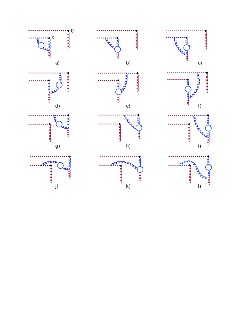
Figure 6: Quark loop correction to gluon TMD evolution.

fffff The quark-loop contribution to the gluon propagator in the bF gauge has the form

$$\langle{\rm T}\{A^{a}_{\mu}(x)A^{b}_{\nu}(y)\}\rangle_{\rm quark~{}loop}$$

$$=~{}\int\!dz_{1}dz_{2}(x|{1\over P^{2}g_{\mu\alpha}+2i{\cal F}_{\mu\alpha}}|z_{1})^{am}{\rm Tr}~{}t^{m}\gamma_{\alpha}(z_{1}|{1\over\not{P}}|z_{2})t^{n}\gamma_{\beta}(z_{2}|{1\over\not{P}}|z_{1})(z_{2}|{1\over P^{2}g_{\beta\nu}+2i{\cal F}_{\beta\nu}}|y)^{nb}$$ (103)

which we need to calculate near the light cone $(x-y)^{2}=0$ in the background field with the only component

$${\cal F}^{-i}(x^{+})$$ (104)

with one-${\cal F}$ accuracy. The relevant diagrams for the gluon propagator are shown in Fig. 7.

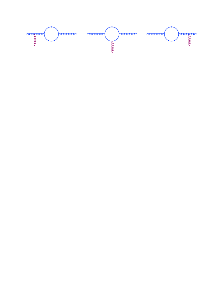
Figure 7: Quark loop correction to the gluon propagator in the background field.

We start from the calculation of the light-cone expansion of the quark loop. Using light-cone expansion of a quark propagator Balitsky:1987bk

$$(z_{1}|{1\over\hat{P}}|z_{2})$$

$$=~{}{\not{z}_{12}\Gamma\big{(}{d\over 2}\big{)}[z_{1},z_{2}]\over 2\pi^{2}(-\Delta^{2})^{d\over 2}}+{g\Gamma\big{(}{d\over 2}-1\big{)}\over 16\pi^{2}(-z_{12}^{2})^{{d\over 2}-1}}\!\int_{0}^{1}\!du~{}[z_{1},z_{u}]\big{(}{\bar{u}}\not{z}_{12}\sigma{\cal F}(z_{u})+u\sigma{\cal F}(z_{u})\not{z}_{12}\big{)}[z_{u},z_{2}]~{}+~{}O(D^{\mu}{\cal F}_{\mu\nu},{\cal F}^{2})$$ (105)

where ${\bar{u}}\equiv 1-u$ and $z_{u}\equiv uz_{1}+{\bar{u}}z_{2}$, we get

$${\rm Tr}~{}t^{a}\gamma_{\alpha}(z_{1}|{1\over\hat{P}}|z_{2})t^{b}\gamma_{\beta}(z_{2}|{1\over\hat{P}}|z_{1})~{}$$

$$=~{}i{B\big{(}{d\over 2},{d\over 2}\big{)}\over 4\pi^{d\over 2}4^{-{\varepsilon}}}[z_{1},z_{2}]^{ab}(z_{1}|(p^{2}g_{\alpha\beta}-p_{\alpha}p_{\beta}){\Gamma(-{\varepsilon})\over(-p^{2})^{-{\varepsilon}}}|z_{2})~{}$$

$$+~{}{B\big{(}{d\over 2},{d\over 2}-1\big{)}\over 8\pi^{d}}{g\Gamma(d-1)\over(-z_{12}^{2})^{d-1}}\!\int_{0}^{1}\!du~{}\Big{(}[z_{1},z_{u}]z_{12}^{\xi}z_{12}^{\eta}\big{(}2i{\bar{u}}g_{\alpha\xi}{\cal F}_{\beta\eta}(z_{u})-2iug_{\beta\xi}{\cal F}_{\alpha\eta}(z_{u})+iz_{12}^{2}{\cal F}_{\alpha\beta}(z_{u})\big{)}[z_{u},z_{2}]\Big{)}^{ab}$$ (106)

where $B(a,b)=\Gamma(a)\Gamma(b)/\Gamma(a+b)$ and ${\varepsilon}\equiv{d\over 2}-2$. To perform integration over $z_{1}$ and $z_{2}$ in Eq. (103), it is convenient to use Eq. (175) from the Appendix VII.4 (at $a=-{\varepsilon}$) and represent Eq. (106) as follows

$${\rm Tr}~{}t^{a}\gamma_{\alpha}(x|{1\over\hat{P}}|0)t^{b}\gamma_{\beta}(0|{1\over\hat{P}}|x)~{}=~{}$$

$$=~{}i{B\big{(}{d\over 2},{d\over 2}\big{)}\over\pi^{d\over 2}4^{1+{\varepsilon}}}\Big{\{}(z_{1}|(P^{2}g_{\alpha\beta}{\Gamma(-{\varepsilon})\over(-P^{2})^{-{\varepsilon}}}-P_{\alpha}{\Gamma\big{(}-{\varepsilon})\over(-P^{2})^{-{\varepsilon}}}P_{\beta})|z_{2})~{}$$

$$+~{}ig(z_{1}|{\Gamma(-{\varepsilon})\over(-p^{2})^{-{\varepsilon}}}|0)\!\int_{0}^{1}\!du~{}{\cal F}_{\alpha\beta}(z_{u})\Big{[}d-2+{d-4\over 2(d-2)}\Big{]}+{gd\over d-2}(z_{1}|{p^{\xi}\Gamma(1-{\varepsilon})\over(-p^{2})^{1-{\varepsilon}}}|z_{2})\!\int_{0}^{1}\!du~{}{\bar{u}}u(D_{\alpha}{\cal F}_{\beta\xi}(z_{u})+\alpha\leftrightarrow\beta)$$

$$+~{}{2ig\over d-2}\!\int_{0}^{1}\!du~{}\Big{[}-up^{\xi}\Big{(}{\cal F}_{\alpha\xi}(z_{u})(z_{1}|{\Gamma(1-{\varepsilon})\over(-p^{2})^{1+{\varepsilon}}}|z_{2})\Big{)}\stackrel{{\scriptstyle\leftarrow}}{{p}}_{\beta}+{\bar{u}}p_{\alpha}\Big{(}{\cal F}_{\beta\xi}(z_{u})(z_{1}|{\Gamma(1-{\varepsilon})p^{\xi}\over(-p^{2})^{1-{\varepsilon}}}|z_{2})\Big{)}\Big{]}\Big{\}}~{}+~{}O(D{\cal F},{\cal F}^{2})$$ (107)

Subtracting the counterterm

$${1\over 2}\delta Z_{3}^{F}A^{a\mu}\big{(}D^{2}g_{\mu\nu}-2i{\cal F}_{\mu\nu}-D_{\mu}D_{\nu}\big{)}^{ab}A^{b}_{\nu}$$

where $\delta Z_{3}^{F}={g^{2}\over 24\pi^{2}{\varepsilon}}$, we get

$$g^{2}{\rm Tr}~{}t^{a}\gamma_{\alpha}(z_{1}|{1\over\hat{P}}|z_{2})t^{b}\gamma_{\beta}(z_{2}|{1\over\hat{P}}|z_{1})~{}-~{}{\rm counterterm}$$ (108)

$$=~{}{ig^{2}\over 4\pi^{2}}\Big{\{}g_{\alpha\beta}(z_{1}|P^{2}\ln{\tilde{\mu}^{2}\over-P^{2}}|z_{2})-(z_{1}|P_{\alpha}\ln{\tilde{\mu}^{2}\over-P^{2}}P_{\beta}|z_{2})+ig\!\int_{0}^{1}\!du~{}\Big{[}u\Big{(}{\cal F}_{\alpha\xi}(z_{u})(z_{1}|{p^{\xi}\over p^{2}}|z_{2})\Big{)}\stackrel{{\scriptstyle\leftarrow}}{{P}}_{\beta}$$

$$\hskip 5.69054pt-P_{\alpha}\Big{(}{\bar{u}}{\cal F}_{\beta\xi}(z_{u})(z_{1}|{p^{\xi}\over p^{2}}|z_{2})\Big{)}+~{}(z_{1}|2\ln{\tilde{\mu}^{2}\over-p^{2}}-{5\over 2}|z_{2}){\cal F}_{\alpha\beta}(z_{u})+2i{\bar{u}}u(z_{1}|{p^{\xi}\over p^{2}}|z_{2})(D_{\alpha}{\cal F}_{\beta\xi}(z_{u})+\alpha\leftrightarrow\beta)\Big{]}\Big{\}}$$

(recall that $\tilde{\mu}^{2}\equiv\bar{\mu}^{2}_{\rm MS}e^{5/3}$). Substituting this expression to Eq. (103), we obtain

$$\langle{\rm T}\{A^{a}_{\mu}(x)A^{b}_{\nu}(y)\}\rangle_{\rm quark~{}loop}~{}=~{}{g^{2}\over 24\pi^{2}}\Big{\{}ig_{\mu\nu}(x|{\ln-\tilde{\mu}^{2}/P^{2}\over P^{2}}|y)-i(x|P_{\mu}{\ln-\tilde{\mu}^{2}/P^{2}\over P^{4}}P_{\nu}|y)+2g(x|{1\over p^{2}}\big{\{}{\cal F}_{\mu\nu},\ln{\tilde{\mu}^{2}\over-p^{2}}\big{\}}{1\over p^{2}}|y)$$

$$\hskip 14.22636pt+~{}g\!\int\!dz_{1}dz_{2}\!\int_{0}^{1}\!du~{}\Big{[}-u(x|{1\over p^{2}}]z_{1}){\cal F}_{\mu\xi}(z_{u})(z_{1}|{p^{\xi}\over p^{2}}|z_{2})(z_{2}|{p_{\nu}\over p^{2}}|y)+{\bar{u}}(x|{p_{\mu}\over p^{2}}]z_{1}){\cal F}_{\nu\xi}(z_{u})(z_{1}|{p^{\xi}\over p^{2}}|z_{2})(z_{2}|{1\over p^{2}}|y)$$

$$\hskip 28.45274pt-~{}(x|{1\over p^{2}}|z_{1})\Big{(}2i{\bar{u}}u(z_{1}|{p^{\xi}\over p^{2}}|z_{2})(D_{\mu}{\cal F}_{\nu\xi}(z_{u})+\mu\leftrightarrow\nu)+(z_{1}|2\ln{\tilde{\mu}^{2}\over-p^{2}}-{5\over 2}|z_{2}){\cal F}_{\mu\nu}(z_{u})\Big{)}(z_{2}|{1\over p^{2}}|y)\Big{]}\Big{\}}$$ (109)

for one flavor of massless quarks. We will need also

$$\langle{\rm T}\{A^{a}_{\alpha}(x)F^{b}_{\mu\nu}(y)\}\rangle_{\rm quark~{}loop}~{}=~{}{g^{2}\over 24\pi^{2}}\Big{\{}-g_{\alpha\nu}(x|{\ln{\tilde{\mu}^{2}\over-P^{2}}\over P^{2}}P_{\mu}|y)+2ig(x|{1\over p^{2}}\big{\{}{\cal F}_{\alpha\nu},\ln{\tilde{\mu}^{2}\over-p^{2}}\big{\}}{p_{\mu}\over p^{2}}|y)$$

$$\hskip 14.22636pt+~{}{ig\over 2}(x|p_{\alpha}{\ln{\tilde{\mu}^{2}\over-p^{2}}\over p^{4}}{\cal F}_{\mu\nu}|y)+~{}\!\int\!dz_{1}dz_{2}\!\int_{0}^{1}\!du~{}\Big{[}i{\bar{u}}(x|{p_{\alpha}\over p^{2}}]z_{1}){\cal F}_{\nu\xi}(z_{u})(z_{1}|{p^{\xi}\over p^{2}}|z_{2})(z_{2}|{p_{\mu}\over p^{2}}|y)$$ (110)

$$\hskip 28.45274pt-~{}ig(x|{1\over p^{2}}|z_{1})\Big{(}2i{\bar{u}}u(z_{1}|{p^{\xi}\over p^{2}}|z_{2})(D_{\alpha}{\cal F}_{\nu\xi}(z_{u})+\alpha\leftrightarrow\nu)+(z_{1}|2\ln{\tilde{\mu}^{2}\over-p^{2}}-{5\over 2}|z_{2}){\cal F}_{\alpha\nu}(z_{u})\Big{)}(z_{2}|{p_{\mu}\over p^{2}}|y)\Big{]}\Big{\}}-\mu\leftrightarrow\nu$$

Let us calculate now the quark-loop contribution to Eq. (85). As we discussed above, we can put $x^{+}=y^{+}=0$ and $y_{\perp}=0$,

$$\delta^{-}{d\over d\delta^{-}}\langle{\rm T}\{F^{-i,a}(0^{+},x_{\perp},-\delta^{\prime-})[x^{+},-\infty^{+}]_{x}^{ac}[-\infty^{+},0^{+}]^{cd}F^{-,d}_{~{}~{}i}(0^{+},0_{\perp},-\delta^{-})\}\rangle_{\cal A}$$ (111)

We start with the term coming from the diagram in Fig. 6(j)-6(l);

$$\delta^{-}{d\over d\delta^{-}}\langle{\rm T}\{[0^{+},-\infty^{+}]_{x}^{ac}~{}[-\infty^{+},0^{+}]^{cd}F^{-,d}_{~{}~{}i}(0^{+},0_{\perp},-\delta^{-})\}\rangle_{\cal A}$$

$$\hskip 14.22636pt=~{}-gf^{abc}\delta^{-}{d\over d\delta^{-}}\!\int_{-\infty}^{0}\!dz^{+}\langle A^{-b}(z^{+},0^{-},x_{\perp})F^{-,c}_{~{}~{}i}(0^{+},0_{\perp},-\delta^{-})~{}-~{}(x_{\perp}\rightarrow 0)\rangle_{\cal A}$$ (112)

First, let us demonstrate that the terms in the second line in Eq. (110) do not contribute to Eq. (112). Indeed, consider, for example, the first term

$$\delta^{-}{d\over d\delta^{-}}\!\int_{-\infty}^{0}\!dz^{+}(0^{-},z^{+},x^{\perp}|p^{-}{\ln{\tilde{\mu}^{2}\over-p^{2}}\over p^{4}}|0^{+},y_{\perp},-\delta^{-}){\cal F}^{-}_{~{}i}(0^{+},y_{\perp})-(x_{\perp}\rightarrow 0)$$

$$\hskip 14.22636pt=~{}\delta^{-}{d\over d\delta^{-}}(0^{-},0^{+},x^{\perp}|{\ln{\tilde{\mu}^{2}\over-p^{2}}\over p^{4}}|0^{+},0_{\perp},-\delta^{-}){\cal F}^{-}_{~{}i}(0^{+},0_{\perp})-(x_{\perp}\rightarrow 0)~{}=~{}0$$ (113)

because $(0,0^{+},x^{\perp}|{\ln{\tilde{\mu}^{2}\over-p^{2}}\over p^{4}}|0^{+},0_{\perp},-\delta^{-})$ does not depend on $\delta^{-}$. Similarly, for the second term in the second line of Eq. (110) one gets

$$\delta^{-}{d\over d\delta^{-}}\!\int_{-\infty}^{0}\!dz^{+}\!\int_{0}^{1}\!du~{}{\bar{u}}\Big{[}(0^{-},z^{+},x^{\perp}|{p^{-}\over p^{2}}]z_{1}){\cal F}_{\nu\xi}(z_{u})(z_{1}|{p^{\xi}\over p^{2}}|z_{2})(z_{2}|{p_{\mu}\over p^{2}}|0^{+},0_{\perp},-\delta^{-})~{}-~{}(\mu\leftrightarrow\nu)-(x_{\perp}\rightarrow 0)\Big{]}$$

$$=~{}\delta^{-}{d\over d\delta^{-}}\!\int_{0}^{1}\!du~{}{\bar{u}}\Big{[}(0^{-},0^{+},x^{\perp}|{1\over p^{2}}]z_{1}){\cal F}_{\nu\xi}(z_{u})(z_{1}|{p^{\xi}\over p^{2}}|z_{2})(z_{2}|{p_{\mu}\over p^{2}}|0^{+},0_{\perp},-\delta^{-})~{}-~{}(\mu\leftrightarrow\nu)~{}-~{}(x_{\perp}\rightarrow 0)\Big{]}$$

$$=~{}\delta^{-}{d\over d\delta^{-}}\Big{[}{i(x_{\perp}+\delta^{-})_{\mu}(x_{\perp}+\delta^{-})^{\xi}\over 16\pi^{2}x_{\perp}^{2}}\!\int_{0}^{1}\!du~{}u\ln u~{}{\cal F}_{\nu\xi}(0^{+})~{}-~{}(\mu\leftrightarrow\nu)+{i\over 32\pi^{d\over 2}}{\Gamma({\varepsilon})\over(x_{\perp}^{2})^{{\varepsilon}}}\!\int_{0}^{1}\!du~{}(\ln u+{\bar{u}}u)~{}{\cal F}_{\mu\nu}(0)$$

$$~{}-~{}(x_{\perp}\rightarrow 0)\Big{]}~{}=~{}~{}-{1\over 64\pi^{2}}{\cal F}_{\nu j}(0)\delta^{-}{d\over d\delta^{-}}\Big{[}{i(x_{\perp}+\delta^{-})_{\mu}x_{\perp}^{j}\over x_{\perp}^{2}}~{}-~{}(\mu\leftrightarrow\nu)\Big{]}$$ (114)

where we used Eq. (185) from the Appendix VII.5 and the fact that $D^{\xi}{\cal F}_{\nu\xi}=0$ for our background field. Now, we have either ($\mu=i,\nu=-$) or vice versa. In the first case nothing in square brackets depends on $\delta^{-}$ while in the second case ${\cal F}_{ij}=0$ for our background field (104).

Thus, the second line in Eq. (110) can be ignored and we get

$$\delta^{-}{d\over d\delta^{-}}g\langle{\rm T}\{[x^{+},-\infty]_{x}^{ac}[-\infty,y^{+}]_{y}^{cd}F^{-i,d}(0^{+},0_{\perp},-\delta^{-})\}\rangle_{\cal A}$$

$$=~{}{g^{2}\over 24\pi^{2}}iN_{c}\delta^{-}{d\over d\delta^{-}}\!\int_{-\infty}^{0}\!dz^{+}\Big{\{}2i(z^{+},x_{\perp},0^{-}|{1\over p^{2}}\big{\{}{\cal F}^{-i,a},\ln{\tilde{\mu}^{2}\over-p^{2}}\big{\}}{p^{-}\over p^{2}}|y_{\delta})$$

$$-~{}\!\int\!dz_{1}dz_{2}\!\int_{0}^{1}\!du~{}(z^{+},x_{\perp},0^{-}|{1\over p^{2}}|z_{1})\Big{[}i(z_{1}|2\ln{\tilde{\mu}^{2}\over-p^{2}}-{5\over 2}|z_{2}){\cal F}^{-i,a}(z_{u})(z_{2}|{p^{-}\over p^{2}}|y_{\delta})$$

$$+~{}2{\bar{u}}u(z_{1}|{p^{+}\over p^{2}}|z_{2})D^{-}{\cal F}^{-,i}(z_{u})(z_{2}|{p^{-}\over p^{2}}|y_{\delta})+~{}4{\bar{u}}u(z_{1}|{p_{j}\over p^{2}}|z_{2})D^{-}{\cal F}^{-j,a}(z_{u})(z_{2}|{p^{i}\over p^{2}}|y_{\delta})\Big{]}~{}-~{}(x_{\perp}\rightarrow 0)$$ (115)

where $|y_{\delta})\equiv|0^{+},0_{\perp},-\delta^{-})$.

The first contribution to RHS of Eq. (115) is proportional to

$$\delta^{-}{d\over d\delta^{-}}\!\int_{-\infty}^{0}\!dz^{+}\Big{(}2i(z^{+},x_{\perp},0^{-}|{1\over p^{2}}\big{\{}{\cal F}^{-,i},\ln{\tilde{\mu}^{2}\over-p^{2}}\big{\}}{p^{-}\over p^{2}}|0^{+},0_{\perp},-\delta^{-})$$ (116)

$$-~{}i\!\int\!dz_{1}dz_{2}\!\int_{0}^{1}\!du~{}(z^{+},x_{\perp},0^{-}|{1\over p^{2}}|z_{1})(z_{1}|2\ln{\tilde{\mu}^{2}\over-p^{2}}-{5\over 2}|z_{2}){\cal F}^{-,i}(z_{u})(z_{2}|{p^{-}\over p^{2}}|0^{+},0_{\perp},-\delta^{-})~{}-~{}(x_{\perp}\rightarrow 0)\Big{)}$$

$$~{}=~{}\delta^{-}{d\over d\delta^{-}}\Big{[}-2(0^{+},x_{\perp},0^{-}|{1\over p^{2}}\big{\{}{\cal F}^{-,i},\ln{\tilde{\mu}^{2}\over-p^{2}}\big{\}}{1\over p^{2}}|0^{+},0_{\perp},-\delta^{-})$$

$$+~{}\!\int\!dz_{1}dz_{2}\!\int_{0}^{1}\!du~{}(0^{+},x_{\perp},0^{-}|{1\over p^{2}}|z_{1})(z_{1}|2\ln{\tilde{\mu}^{2}\over-p^{2}}-{5\over 2}|z_{2}){\cal F}^{-,i}(z_{u})(z_{2}|{1\over p^{2}}|0^{+},0_{\perp},-\delta^{-})~{}-~{}(x_{\perp}\rightarrow 0)\Big{]}$$

$$+~{}\delta^{-}{d\over d\delta^{-}}\!\int_{-\infty}^{0}\!dz^{+}\Big{(}2(z^{+},x_{\perp},0^{-}|{1\over p^{2}}\big{\{}D^{-}{\cal F}^{-,i},\ln{\tilde{\mu}^{2}\over-p^{2}}\big{\}}{1\over p^{2}}|0^{+},0_{\perp},-\delta^{-})$$

$$-~{}\!\int\!dz_{1}dz_{2}\!\int_{0}^{1}\!du~{}(z^{+},x_{\perp},0^{-}|{1\over p^{2}}|z_{1})(z_{1}|2\ln{\tilde{\mu}^{2}\over-p^{2}}-{5\over 2}|z_{2})D^{-}{\cal F}^{-,i}(z_{u})(z_{2}|{1\over p^{2}}|0^{+},0_{\perp},-\delta^{-})~{}-~{}(x_{\perp}\rightarrow 0)\Big{)}\,,$$

where we used Eq. (190). Similar to Eq. (113), the first term in the RHS vanishes since the expression in the square brackets does not actually depend on $\delta^{-}$. Using Eqs. (177), (178), and (169), the second term can be rewritten as

$${\rm RHS~{}of~{}Eq.~{}(\ref{firstem1})}~{}=~{}\delta^{-}{d\over d\delta^{-}}\!\int_{-\infty}^{0}\!dz^{+}\!\int_{0}^{1}\!du\Big{[}(z^{+},x_{\perp},0^{-}|{2\ln{\tilde{\mu}^{2}\over-p^{2}}+{9\over 2}\over p^{4}}|0^{+},0_{\perp},-\delta^{-})~{}D^{-}{\cal F}^{-,i}(uz^{+})~{}-~{}(x_{\perp}\rightarrow 0)\Big{]}$$

$$=~{}-\!\int_{-\infty}^{0}\!dz^{+}D^{-}{\cal F}^{-,i}(z^{+})\Big{[}(z^{+},x_{\perp},0^{-}|{2\ln{\tilde{\mu}^{2}\over-p^{2}}+{9\over 2}\over p^{4}}|0^{+},0_{\perp},-\delta^{-})~{}-~{}(x_{\perp}\rightarrow 0)\Big{]}$$

$$=~{}-{i\over 8\pi^{2}}\!\int_{-\infty}^{0}\!dz^{+}D^{-}{\cal F}^{-,i}(z^{+})\Big{[}{\Gamma({\varepsilon})\over(x_{\perp}^{2}-2z^{+}\delta^{-})^{\varepsilon}}\Big{(}{1\over{\varepsilon}}+\ln{\tilde{\mu}^{2}(x_{\perp}^{2}-2z^{+}\delta^{-})\over 4}~{}-~{}\psi(1+{\varepsilon})+\gamma+{5\over 4}\Big{)}~{}-~{}(x_{\perp}\rightarrow 0)\Big{]}$$

$$=~{}{i\over 16\pi^{2}}\!\int_{-\infty}^{0}\!dz^{+}D^{-}{\cal F}^{-,i}(z^{+})\ln{x_{\perp}^{2}-2z^{+}\delta^{-}\over-2z^{+}\delta^{-}}\Big{[}\ln\tilde{\mu}^{2}{x_{\perp}^{2}-2z^{+}\delta^{-}\over 4}+\ln\tilde{\mu}^{2}{-2z^{+}\delta^{-}\over 4}+4\gamma+{5\over 2}\Big{]}$$ (117)

We get

$${g^{2}\over 24\pi^{2}}iN_{c}\delta^{-}{d\over d\delta^{-}}\!\int_{-\infty}^{0}\!dz^{+}\Big{[}2i(z^{+},x_{\perp},0^{-}|{1\over p^{2}}\big{\{}{\cal F}^{-,i},\ln{\tilde{\mu}^{2}\over-p^{2}}\big{\}}{p^{-}\over p^{2}}|y_{\delta})$$

$$-~{}i\!\int\!dz_{1}dz_{2}\!\int_{0}^{1}\!du~{}(z^{+},x_{\perp},0^{-}|{1\over p^{2}}|z_{1})(z_{1}|2\ln{\tilde{\mu}^{2}\over-p^{2}}-{5\over 2}|z_{2}){\cal F}^{-,i}(z_{u})(z_{2}|{p^{-}\over p^{2}}|y_{\delta})~{}-~{}(x_{\perp}\rightarrow 0)\Big{]}$$

$$=~{}-{g^{2}N_{c}\over 384\pi^{2}}\!\int_{-\infty}^{0}\!dz^{+}D^{-}{\cal F}^{-i}(z^{+})\ln{x_{\perp}^{2}-2z^{+}\delta^{-}\over-2z^{+}\delta^{-}}\Big{[}\ln\tilde{\mu}^{2}{x_{\perp}^{2}-2z^{+}\delta^{-}\over 4}+\ln\tilde{\mu}^{2}{-2z^{+}\delta^{-}\over 4}+4\gamma+{5\over 2}\Big{]}$$ (118)

Let us now consider the two remaining terms in the RHS of Eq. (115). With our accuracy the last term in the RHS of Eq. (115) reduces to

$$\delta^{-}{d\over d\delta^{-}}\!\int_{-\infty}^{0}\!dz^{+}\!\int\!dz_{1}dz_{2}\!\int_{0}^{1}\!du~{}{\bar{u}}u(z^{+},x_{\perp},0^{-}|{1\over p^{2}}|z_{1})(z_{1}|{p^{j}\over p^{2}}|z_{2})D^{-}{\cal F}_{-j}(z_{u})(z_{2}|{p^{i}\over p^{2}}|0^{+},0_{\perp},-\delta^{-})~{}-~{}(x_{\perp}\rightarrow 0)$$

$$=~{}-i{\partial\over\partial y_{i}}\delta^{-}{d\over d\delta^{-}}\!\int_{-\infty}^{0}\!dz^{+}\!\int\!dz_{1}dz_{2}\!\int_{0}^{1}\!du~{}{\bar{u}}u(z^{+},x_{\perp},0^{-}|{1\over p^{2}}|z_{1})(z_{1}|{p_{j}\over p^{2}}|z_{2})D^{-}{\cal F}^{-j}(z_{u})(z_{2}|{1\over p^{2}}|0^{+},y_{\perp},-\delta^{-})\Big{|}_{y_{\perp}=0}$$

$$~{}-~{}(x_{\perp}\rightarrow 0)$$

$$=~{}i{1\over 64\pi^{d\over 2}}\delta^{-}{d\over d\delta^{-}}\!\int_{-\infty}^{0}\!dz^{+}\!\int_{0}^{1}\!du~{}{\bar{u}}u\Big{[}{g_{ij}\Gamma({\varepsilon})\over(x_{\perp}^{2}-2z^{+}\delta^{-})^{\varepsilon}}+{2x_{i}x_{j}\over x_{\perp}^{2}-2z^{+}\delta^{-}}\Big{]}D^{-}{\cal F}^{-j}(uz^{+})~{}-~{}(x_{\perp}\rightarrow 0)$$

$$=~{}i{1\over 64\pi^{2}}\!\int_{-\infty}^{0}\!dz^{+}\!\int_{0}^{1}\!du~{}\Big{[}{g_{ij}{\bar{u}}ux_{\perp}^{2}\over ux_{\perp}^{2}-2z^{+}\delta^{-}}+2u(1-2u){x_{i}x_{j}\over ux_{\perp}^{2}-2z^{+}\delta^{-}}\Big{]}D^{-}{\cal F}^{-j}(z^{+})$$ (119)

where we used Eq. (181) to get the fourth line and Eq. (186) to get the last line. As we discussed above, the characteristic $z^{+}$ are $z^{+}_{\rm char}\sim{1\over\beta_{B}{\varrho}}$ so $x_{\perp}^{2}\gg 2z^{+}_{\rm char}\delta^{-}$, and we get

$${g^{2}\over 24\pi^{2}}iN_{c}\delta^{-}{d\over d\delta^{-}}\!\int_{-\infty}^{0}\!dz^{+}\!\int\!dz_{1}dz_{2}\!\int_{0}^{1}\!du~{}\Big{[}4{\bar{u}}u(z_{1}|{p_{j}\over p^{2}}|z_{2})(D^{-}{\cal F}^{-j}(z_{u})(z_{2}|{p^{i}\over p^{2}}|y_{\delta})~{}-~{}(x_{\perp}\rightarrow 0)\Big{]}$$

$$=~{}-{g^{2}N_{c}\over 768\pi^{2}}\!\int_{-\infty}^{0}\!dz^{+}D^{-}{\cal F}^{-i}(z^{+})~{}+~{}O\Big{(}{z^{+}_{\rm char}\delta^{-}\over x_{\perp}^{2}}\Big{)}=~{}-{g^{2}N_{c}\over 768\pi^{2}}{\cal F}^{-i}(0^{+})~{}+~{}O\Big{(}{m_{\perp}^{2}\over\sigma\beta_{B}s}\Big{)}$$ (120)

Finally, from Eq. (189) we get

$$\delta^{-}{d\over d\delta^{-}}\!\int_{-\infty}^{0}\!dz^{+}\!\int\!dz_{1}dz_{2}\!\int_{0}^{1}\!du~{}{\bar{u}}u(z^{+},x_{\perp},0^{-}|{1\over p^{2}}|z_{1})(z_{1}|{p^{+}\over p^{2}}|z_{2})D^{-}{\cal F}^{-,i}(z_{u})(z_{2}|{p^{-}\over p^{2}}|0^{+},0_{\perp},-\delta^{-})~{}-~{}(x_{\perp}\rightarrow 0)$$

$$=~{}-i{\partial\over\partial y^{+}}\delta^{-}{d\over d\delta^{-}}\!\int_{-\infty}^{0}\!dz^{+}\!\int\!dz_{1}dz_{2}\!\int_{0}^{1}\!du~{}{\bar{u}}u(z^{+},x_{\perp},0^{-}|{1\over p^{2}}|z_{1})(z_{1}|{p^{+}\over p^{2}}|z_{2})D^{-}{\cal F}^{-,i}(z_{u})$$

$$\hskip 62.59605pt\times~{}(z_{2}|{1\over p^{2}}|y^{+},0_{\perp},-\delta^{-})\Big{|}_{y^{+}=0}~{}-~{}(x_{\perp}\rightarrow 0)$$

$$=~{}-i{\partial\over\partial y^{+}}\delta^{-}{d\over d\delta^{-}}\!\int_{-\infty}^{0}\!dz^{+}\!\int_{0}^{1}\!du~{}{\bar{u}}u~{}(z^{+},x_{\perp},0^{-}|{p^{+}\over p^{6}}|y^{+},0_{\perp},-\delta^{-})D^{-}{\cal F}^{-,i}(uz^{+}+{\bar{u}}y^{+})\Big{|}_{y^{+}=0}~{}-~{}(x_{\perp}\rightarrow 0)$$

$$=~{}i\delta^{-}{d\over d\delta^{-}}\!\int_{-\infty}^{0}\!dz^{+}{\partial\over\partial z^{+}}\!\int_{0}^{1}\!du~{}{\bar{u}}u~{}(z^{+},x_{\perp},0^{-}|{p^{+}\over p^{6}}|0^{+},0_{\perp},-\delta^{-})D^{-}{\cal F}^{-,i}(uz^{+})~{}-~{}(x_{\perp}\rightarrow 0)$$

$$-~{}i\delta^{-}{d\over d\delta^{-}}\!\int_{-\infty}^{0}\!dz^{+}\!\int_{0}^{1}\!du~{}{\bar{u}}u~{}(z^{+},x_{\perp},0^{-}|{p^{+}\over p^{6}}|0^{+},0_{\perp},-\delta^{-})(D^{-})^{2}{\cal F}^{-,i}(uz^{+})~{}-~{}(x_{\perp}\rightarrow 0)$$

$$=~{}-~{}i\delta^{-}{d\over d\delta^{-}}\!\int_{-\infty}^{0}\!dz^{+}\!\int_{0}^{1}\!du~{}{\bar{u}}u~{}(z^{+},x_{\perp},0^{-}|{p^{+}\over p^{6}}|0^{+},0_{\perp},-\delta^{-})(D^{-})^{2}{\cal F}^{-,i}(uz^{+})~{}-~{}(x_{\perp}\rightarrow 0)$$ (121)

because the term in the fifth line vanishes similar to Eq. (113). Using the first of Eqs. (186) with ${\cal O}(uz^{+})=uz^{+}(D^{-})^{2}{\cal F}^{-,i}(uz^{+})$, we obtain

$${\rm RHS~{}of~{}Eq.~{}(\ref{poldela})}~{}=~{}-i{1\over 64\pi^{2}}\!\int_{-\infty}^{0}\!dz^{+}(D^{-})^{2}{\cal F}^{-,i}(z^{+})\!\int_{0}^{1}\!du~{}z_{+}\ln{ux_{\perp}^{2}-2z^{+}\delta^{-}\over-2z^{+}\delta^{-}}$$

$$=~{}{i\over 64\pi^{2}}\!\int_{-\infty}^{0}\!dz^{+}D^{-}{\cal F}^{-,i}(z^{+})\!\int_{0}^{1}\!du~{}\Big{[}\ln{ux_{\perp}^{2}-2z^{+}\delta^{-}\over-2z^{+}\delta^{-}}-{ux_{\perp}^{2}\over ux_{\perp}^{2}-2z^{+}\delta^{-}}\Big{]}$$

$$=~{}{i\over 64\pi^{2}}\!\int_{-\infty}^{0}\!dz^{+}D^{-}{\cal F}^{-,i}(z^{+})\Big{[}\ln{x_{\perp}^{2}\over-2z^{+}\delta^{-}}-2\Big{]}~{}+~{}O\Big{(}{m_{\perp}^{2}\over\sigma\beta_{B}s}\Big{)}$$ (122)

because the characteristic $z^{+}$ are $\sim{1\over\beta_{B}{\varrho}}$. Thus, the first term in the last line in Eq. (115) is

$${g^{2}\over 24\pi^{2}}iN_{c}\delta^{-}{d\over d\delta^{-}}\!\int_{-\infty}^{0}\!dz^{+}\!\int\!dz_{1}dz_{2}\!\int_{0}^{1}\!du~{}2{\bar{u}}u(z_{1}|{p^{+}\over p^{2}}|z_{2})(D^{-}{\cal F}^{-,i}(z_{u})(z_{2}|{p^{-}\over p^{2}}|0^{+},0_{\perp},-\delta^{-})~{}-~{}(x_{\perp}\rightarrow 0)$$

$$=~{}-{g^{2}N_{c}\over 768\pi^{4}}\!\int_{-\infty}^{0}\!dz^{+}D^{-}{\cal F}^{-i}(z^{+})\Big{[}\ln{x_{\perp}^{2}\over-2z^{+}\delta^{-}}-2\Big{]}~{}+~{}O\Big{(}{m_{\perp}^{2}\over\sigma\beta_{B}s}\Big{)}$$ (123)

Let us now assemble the result for the contribution (112) given by a sum of Eqs. (118), (123), and (120)

$$\delta^{-}{d\over d\delta^{-}}\langle{\rm T}\{[0^{+},-\infty]_{x}^{ac}~{}[-\infty,0^{+}]_{0}^{cd}F^{-,d}_{~{}~{}i}(0^{+},0_{\perp},-\delta^{-})\}\rangle_{\cal A}$$ (124)

$$=-{g^{2}N_{c}\over 384\pi^{4}}\!\int_{-\infty}^{0}\!\!dz^{+}D^{-}{\cal F}^{-i,a}(z^{+})\Big{\{}\ln{x_{\perp}^{2}-2z^{+}\delta^{-}\over-2z^{+}\delta^{-}}\Big{[}\ln\tilde{\mu}^{2}{x_{\perp}^{2}-2z^{+}\delta^{-}\over 4}+\ln\tilde{\mu}^{2}{-2z^{+}\delta^{-}\over 4}+4\gamma+3\Big{]}-{1\over 2}\Big{\}}~{}+~{}O\Big{(}{m_{\perp}^{2}\over\sigma\beta_{B}s}\Big{)}$$

Note that double-log terms are the same as in the quark case, see Eq. (71).

Performing Fourier transformation using Eqs. (72) and (73) we get

$$\delta^{-}{d\over d\delta^{-}}\langle{\rm T}\{[x^{+},-\infty]_{x}^{ab}[-\infty,0^{+}]_{0}^{bc}F^{-j,c}\big{(}0^{+},0_{\perp},-{1\over{\varrho}\sigma}\big{)}\}\rangle_{\cal A}^{\rm Fig.~{}\ref{fig:gldiagrams}a-c~{}loop}~{}=~{}-{g^{2}N_{c}\over 384\pi^{4}}\!\int\!{\textstyle d}\lower 0.12915pt\hbox{\kern-3.80005pt${}^{\scriptstyle-}$}\kern-0.50003pt{}\beta_{B}~{}e^{-i\beta_{B}{\varrho}y^{+}}$$ (125)

$$\hskip 5.69054pt\times~{}\Big{\{}\Big{(}\ln{x_{\perp}^{2}{\varrho}\over 2\delta^{-}}[-i\beta_{B}+\epsilon]+\gamma\Big{)}\Big{(}\ln{x_{\perp}^{2}\tilde{\mu}^{4}\delta^{-}\over 8{\varrho}(-i\beta_{B}+\epsilon)}+3\gamma+3\Big{)}-{1\over 2}-{\pi^{2}\over 6}~{}+~{}O\Big{(}{m_{\perp}^{2}\over\beta_{B}\sigma s}\Big{)}\Big{\}}{\cal F}^{-i,a}(\beta_{B},0_{\perp})$$

Recall that we calculated the contribution due to one quark flavor, so for $n_{f}$ flavors we should multiply Eq. (125) by $n_{f}$, and to use the BLM prescription we must replace $-{1\over 6\pi}n_{f}$ by $b_{0}={11\over 12\pi}N_{c}-{1\over 6\pi}n_{f}$. We obtain then

$$\sigma^{-}{d\over d\sigma^{-}}\langle{\rm T}\{[x^{+},-\infty]_{x}^{ab}[-\infty,0^{+}]_{0}^{bc}F^{-j,c}\big{(}0^{+},0_{\perp},-{1\over{\varrho}\sigma}\big{)}\}\rangle_{\cal A}^{\rm Fig.~{}\ref{fig:gldiagrams}a-c~{}loop}~{}=~{}-{g^{2}N_{c}b_{0}\over 64\pi^{3}}\!\int\!{\textstyle d}\lower 0.12915pt\hbox{\kern-3.80005pt${}^{\scriptstyle-}$}\kern-0.50003pt{}\beta_{B}~{}e^{-i\beta_{B}{\varrho}y^{+}}$$ (126)

$$\hskip 5.69054pt\times~{}\Big{\{}\Big{(}\ln{x_{\perp}^{2}\sigma s\over 4}[-i\beta_{B}+\epsilon]+\gamma\Big{)}\Big{(}\ln{x_{\perp}^{2}\tilde{\mu}^{4}\over 4\sigma s(-i\beta_{B}+\epsilon)}+3\gamma+3\Big{)}-{1\over 2}-{\pi^{2}\over 6}~{}+~{}O\Big{(}{m_{\perp}^{2}\over\beta_{B}\sigma s}\Big{)}\Big{\}}{\cal F}^{-i,a}(\beta_{B},0_{\perp})$$

Adding the leading-order term and restoring $y^{+},y_{\perp}$ we get

$$\sigma{d\over d\sigma}\langle{\rm T}\{[x^{+},-\infty]_{x}^{ab}[-\infty,y^{+}]_{y}^{bc}F^{-j,c}\big{(}y^{+},y_{\perp},-{1\over{\varrho}\sigma}\big{)}\}\rangle_{\cal A}^{\rm Fig.~{}\ref{fig:gldiagrams}a-c~{}+~{}loop}$$ (127)

$$\hskip 5.69054pt=~{}-{\alpha_{s}(\tilde{\mu})\over 2\pi}N_{c}\!\int\!{\textstyle d}\lower 0.12915pt\hbox{\kern-3.80005pt${}^{\scriptstyle-}$}\kern-0.50003pt{}\beta_{B}~{}{\cal F}^{-j,b}(\beta_{B},y_{\perp})e^{-i\beta_{B}{\varrho}y^{+}}\Big{\{}\ln\Big{(}{\Delta_{\perp}^{2}\over 4}(-i\beta_{B}+\epsilon)\sigma se^{\gamma}\Big{)}~{}+~{}O\big{(}{m_{\perp}^{2}\over\beta_{B}\sigma s}\big{)}$$

$$+~{}{b\alpha_{s}(\tilde{\mu})\over 8\pi}\Big{\{}\Big{(}\ln{\Delta_{\perp}^{2}\sigma s\over 4}[-i\beta_{B}+\epsilon]+\gamma\Big{)}\Big{(}\ln{\Delta_{\perp}^{2}\tilde{\mu}^{4}\over 4\sigma s(-i\beta_{B}+\epsilon)}+3\gamma+3\Big{)}-{1\over 2}-{\pi^{2}\over 6}~{}+~{}O\Big{(}{m_{\perp}^{2}\over\beta_{B}\sigma s}\Big{)}\Big{\}}$$

$$\hskip 5.69054pt=~{}-{\alpha_{s}(\mu_{\sigma})\over 2\pi}N_{c}\!\int\!{\textstyle d}\lower 0.12915pt\hbox{\kern-3.80005pt${}^{\scriptstyle-}$}\kern-0.50003pt{}\beta_{B}{\cal F}^{-j,b}(\beta_{B},y_{\perp})e^{-i\beta_{B}{\varrho}y^{+}}\big{\{}\ln\big{[}-{i\over 4}(\beta_{B}+{i\epsilon})\sigma s\Delta_{\perp}^{2}e^{\gamma}\big{]}+O\big{(}\alpha_{s}(\mu_{\sigma})\big{)}\big{\}}~{}+~{}O\big{(}{m_{\perp}^{2}\over\beta_{B}\sigma s}\big{)}$$

where $\mu^{2}_{\sigma}\equiv\sqrt{\sigma|\beta_{B}|s\over\Delta_{\perp}^{2}}$.

We see that the result is the same as Eq. (59) for tquark TMD up to the replacement $c_{F}\rightarrow N_{c}$ and $O\big{(}\alpha_{s}(\mu_{\sigma})\big{)}$ corrections. Because of that, we can just recycle all formulas for the evolution from the quark TMD case replacing $c_{F}\rightarrow N_{c}$ when appropriate. The evolution equation for gluon TMDs will be

$$\Big{(}\sigma{d\over d\sigma}+\sigma^{\prime}{d\over d\sigma^{\prime}}\Big{)}\mathscr{F}^{i,a;\sigma^{\prime}}(\beta^{\prime}_{B},x_{\perp})\mathscr{F}^{a;\sigma}_{~{}~{}i}(\beta_{B},y_{\perp})$$ (128)

$$\hskip 5.69054pt=~{}-{N_{c}\over 2\pi}\mathscr{F}^{i,a;\sigma^{\prime}}(\beta^{\prime}_{B},x_{\perp})\mathscr{F}^{a;\sigma}_{~{}~{}i}(\beta_{B},y_{\perp})\Big{[}\alpha_{s}(\mu_{\sigma^{\prime}})\ln\Big{(}-{i\over 4}(\beta^{\prime}_{B}+{i\epsilon})\sigma^{\prime}sb_{\perp}^{2}e^{\gamma}\Big{)}+\alpha_{s}(\mu_{\sigma})\ln\Big{(}-{i\over 4}(\beta_{B}+{i\epsilon})\sigma sb_{\perp}^{2}e^{\gamma}\Big{)}\Big{]}$$

where $b_{\perp}\equiv\Delta_{\perp}$ as usual. The solution of this equation is the same as (63) with $c_{F}\rightarrow N_{c}$ replacement

$$\mathscr{F}^{i,a;\sigma^{\prime}}(\beta^{\prime}_{B},x_{\perp})\mathscr{F}^{a;\sigma}_{~{}~{}i}(\beta_{B},y_{\perp})~{}=~{}e^{-{2N_{c}\over\pi b_{0}^{2}}\big{[}\ln{\alpha_{s}(\mu_{\sigma^{\prime}})\over\alpha_{s}(\mu_{\sigma^{\prime}_{0}})}\big{(}{1\over\alpha_{s}(\tilde{b}_{\perp}^{-1})}+\ln[-i(\tau^{\prime}_{B}+{i\epsilon})]\big{)}+{1\over\alpha_{s}(\mu_{\sigma^{\prime}})}-{1\over\alpha_{s}(\mu_{\sigma^{\prime}_{0}})}\big{]}}$$

$$\times~{}e^{-{2N_{c}\over\pi b_{0}^{2}}\big{[}\ln{\alpha_{s}(\mu_{\sigma})\over\alpha_{s}(\mu_{\sigma_{0}})}\big{(}{1\over\alpha_{s}(\tilde{b}_{\perp}^{-1})}+\ln[-i(\tau_{B}+{i\epsilon})]\big{)}+{1\over\alpha_{s}(\mu_{\sigma})}-{1\over\alpha_{s}(\mu_{\sigma_{0}})}\big{]}}\mathscr{F}^{i,a;\sigma^{\prime}_{0}}(\beta^{\prime}_{B},x_{\perp})\mathscr{F}^{a;\sigma_{0}}_{~{}~{}i}(\beta_{B},y_{\perp})$$ (129)

Let us now set $\sigma^{\prime}=\sigma$ and present the final form of the evolution with the rapidity cutoff (cf. Eq. (65))

$$\mathscr{F}^{i,a;\sigma}(\beta^{\prime}_{B},x_{\perp})\mathscr{F}^{a;\sigma}_{~{}~{}i}(\beta_{B},y_{\perp})~{}=~{}e^{-{2N_{c}\over\pi b_{0}^{2}}\big{[}\ln{\alpha_{s}(\mu_{\sigma^{\prime}})\over\alpha_{s}(\mu_{\sigma^{\prime}_{0}})}\big{(}{1\over\alpha_{s}(\tilde{b}_{\perp}^{-1})}+\ln[-i(\tau^{\prime}_{B}+{i\epsilon})]\big{)}+{1\over\alpha_{s}(\mu_{\sigma^{\prime}})}-{1\over\alpha_{s}(\mu_{\sigma^{\prime}_{0}})}\big{]}}$$

$$\times~{}e^{-{2N_{c}\over\pi b_{0}^{2}}\big{[}\ln{\alpha_{s}(\mu_{\sigma})\over\alpha_{s}(\mu_{\sigma_{0}})}\big{(}{1\over\alpha_{s}(\tilde{b}_{\perp}^{-1})}+\ln[-i(\tau_{B}+{i\epsilon})]\big{)}+{1\over\alpha_{s}(\mu_{\sigma})}-{1\over\alpha_{s}(\mu_{\sigma_{0}})}\big{]}}\mathscr{F}^{i,a;\sigma^{\prime}_{0}}(\beta^{\prime}_{B},x_{\perp})\mathscr{F}^{a;\sigma_{0}}_{~{}~{}i}(\beta_{B},y_{\perp})$$ (130)

It should also be mentioned that the result for the evolution of gluon TMDs with gauge links out to $+\infty$ is Eq. (130) with the replacement $-i(\tau_{B}+{i\epsilon})\rightarrow i(\tau_{B}-{i\epsilon})$, the same as in Eq. (81) for quark TMDs.

VI Conclusions

This paper was devoted to the study of the rapidity evolution of quark and gluon TMDs using the small-$x$ methods. As customary for studies of small-$x$ amplitudes, we used a rapidity-only cutoff for longitudinal divergences due to infinite gauge links. With such cutoff for TMDs, there is only one evolution parameter–this rapidity cutoff. However, as we mentioned in the Introduction, the argument the of coupling constant in such an evolution is undetermined at the leading order. To fix it, one needs to go beyond the leading order and employ some additional BLM/renormalon considerations, as was done for NLO BK evolution in Refs. Balitsky:2006wa ; Kovchegov:2006vj . In this paper, we have done such BLM analysis for both quark and gluon TMDs, and the result is very simple: the effective BLM scale for Sudakov evolution is halfway (in the logarithmical scale) between transverse momentum and longitudinal “energy” of TMD.

Let us present the final form of the running-coupling evolution for the cutoff $\varsigma$ such that $\sigma=\sigma^{\prime}={\varsigma\sqrt{2}\over{\varrho}|\Delta_{\perp}|}$. As we mentioned above, in the leading order the evolution with such a cutoff is conformally invariant, see Eq. (44). With the running coupling, the evolution equation for quark TMDs reads ($b_{\perp}\equiv x_{\perp}-y_{\perp}$)

$$\varsigma{d\over d\varsigma}{\bar{\psi}}^{\varsigma}(\beta^{\prime}_{B},x_{\perp})\Gamma\psi^{\varsigma}(\beta_{B},y_{\perp})$$ (131)

$$\hskip 5.69054pt=~{}-{c_{F}\over 2\pi}{\bar{\psi}}^{\varsigma}(\beta^{\prime}_{B},x_{\perp})\Gamma\psi^{\varsigma}(\beta_{B},y_{\perp})\Big{[}\alpha_{s}(\mu^{\prime}_{\varsigma})\ln\Big{(}-{i\over\sqrt{2}}(\beta^{\prime}_{B}+{i\epsilon})\varsigma{\varrho}b_{\perp}e^{\gamma}\Big{)}+\alpha_{s}(\mu_{\varsigma})\ln\Big{(}-{i\over\sqrt{2}}(\beta_{B}+{i\epsilon})\varsigma{\varrho}b_{\perp}e^{\gamma}\Big{)}\Big{]}$$

where $\mu_{\varsigma}=b_{\perp}^{-1}\big{(}|\beta_{B}|{\varrho}\varsigma\sqrt{2}\big{)}^{1/4},~{}\mu^{\prime}_{\varsigma}=b_{\perp}^{-1}\big{(}|\beta^{\prime}_{B}|{\varrho}\varsigma\sqrt{2}\big{)}^{1/4}$ and the solution has the form

$${\bar{\psi}}^{\varsigma}(\beta^{\prime}_{B},x_{\perp})\Gamma\psi^{\varsigma}(\beta_{B},y_{\perp})~{}=~{}e^{-{2c_{F}\over\pi b_{0}^{2}}\big{[}\ln{\alpha_{s}(\mu^{\prime}_{\varsigma})\over\alpha_{s}(\mu^{\prime}_{\varsigma_{0}})}\big{(}{1\over\alpha_{s}(\tilde{b}_{\perp}^{-1})}+\ln[-i\tau^{\prime}_{B}+\epsilon]\big{)}+{1\over\alpha_{s}(\mu^{\prime}_{\varsigma})}-{1\over\alpha_{s}(\mu^{\prime}_{\varsigma_{0}})}\big{]}}$$

$$\times~{}e^{-{2c_{F}\over\pi b_{0}^{2}}\big{[}\ln{\alpha_{s}(\mu_{\varsigma})\over\alpha_{s}(\mu_{\varsigma_{0}})}\big{(}{1\over\alpha_{s}(\tilde{b}_{\perp}^{-1})}+\ln[-i\tau_{B}+\epsilon]\big{)}+{1\over\alpha_{s}(\mu_{\varsigma})}-{1\over\alpha_{s}(\mu_{\varsigma_{0}})}\big{]}}{\bar{\psi}}^{\varsigma_{0}}(\beta^{\prime}_{B},x_{\perp})\Gamma\psi^{\varsigma_{0}}(\beta_{B},y_{\perp})$$ (132)

where $\tilde{b}_{\perp}^{2}={b_{\perp}^{2}\over 2}e^{\gamma/2}$ and $\tau_{B}={\beta_{B}\over|\beta_{B}|},\tau^{\prime}_{B}={\beta^{\prime}_{B}\over|\beta^{\prime}_{B}|}$. As we mentioned above, although formally $\alpha_{s}\ln[-i\tau_{B}+\epsilon]$ exceeds our accuracy, it determines the direction of evolution of operators in the coordinate space: $+$ positions of operators move to the left as a result of evolution, see the discussion after Eq. (43). Consequently, the evolution of quark TMDs with gauge links out to $+\infty$ has the same form (132) but with $\ln[i\tau_{B}+\epsilon]$ [see Eq. (80)], and $+$ positions of operators move to the right.

Another result of our paper is that with BLM scale setting and the rapidity evolution of gluon TMDs has the same form as the one for quark TMDs with trivial replacement $c_{F}\rightarrow N_{c}$ [see e.g., Eq. (130)].

It should be noted that, although we used the small-$x$ methods (rapidity-only factorization, etc.), our results (131) and (132) are correct at any $x_{B}\equiv\beta_{B}$ as long as $\sigma x_{B}s\gg\sim b_{\perp}^{-2}$. The difference between moderate and small $x$ comes at the end point of evolution. As discussed in Ref. Balitsky:2019ayf , the double-log logarithmical evolution ((63) or (130)) can be used until $\sigma x_{B}s\sim b_{\perp}^{-2}$. At this point, if $x_{B}\sim 1$, the situation is similar to Deep Inelastic Scattering (DIS) at moderate $x$ so one should use single-log DGLAP evolution plus some phenomenological models for TMDs based on relations to ordinary PDFs Collins:1984kg ; Collins:2017oxh If, however, $x_{B}\ll 1$, the situation is more like DIS at small $x$ so the BFKL/Balitsky-Kovchegov (BK) evolution should be applicable. A plausible scenario of matching these evolutions is discussed in Appendix VII.7.

Also, we saw that one should be very careful with rapidity cutoff in order not to spoil analytic properties of Feynman diagrams which may bring out the noncancellation of IR divergences. While the “rigid cutoff” $\sigma\gg\alpha$ did not cause any IR problems in the analysis of dipole evolution, we saw that in such an analysis of TMD evolution it is not applicable and one should use “smooth cutoff” $e^{\pm i\alpha/\sigma}$ to avoid IR divergence.

Finally, an obvious outlook is to study the TMD factorization with rapidity-only cutoffs and find the cross section of the Higgs production or the Drell-Yan process at $q_{\perp}\sim$ few GeV in the one-loop approximation using Eq. (130) and the would-be result for the one-loop “coefficient factor”. In addition, at that point it would be possible to compare our result with the two-loop results obtained by CSS method Gutierrez-Reyes:2017glx ; Li:2016axz ; Gehrmann:2014yya ; Gutierrez-Reyes:2018iod . The study is in progress.

VII Appendix

VII.1 Rapidity cutoff and causality

In this appendix we discuss the effects of rapidity cutoff on general properties of Feynman diagrams. As we saw in Sect. II.2, the rigid cutoff does not ensure cancellation between real and virtual gluon emissions while point-splitting cutoff preserves this cancellation. Thus, one should be very careful imposing cutoffs on Feynman diagrams since one may violate properties of causality and unitarity build-in into Feynman diagrams.

It is a textbook subject that perturbative series in a quantum field theory preserve causality so if one calculates diagrams for some commutator at spacelike distances one should get zero as a result. (Some caution must be applied in a gauge theory where this property is correct for gauge-invariant operators.) Similarly, one should expect the same property in a quantum theory in the background field, namely diagrams in the background field for the commutator at spacelike distances should sum up to zero. Let us check this causality property for our typical commutators and discuss whether this property survives our rapidity cutoff for Feynman diagrams.

To avoid the above-mentioned specific complications in gauge theories, we consider a massless scalar theory in the background field described by the Lagrangian

$$L~{}=~{}{1\over 2}\partial^{\mu}{\varphi}\partial_{\mu}{\varphi}+{\lambda\over 2}{\varphi}^{2}{\bar{\phi}}$$

where ${\bar{\phi}}(x)~{}=~{}{\bar{\phi}}(x^{+},x_{\perp})$ is a background scalar field which does not depend on $x^{-}$. Let us calculate the expectation value of the commutator $[\phi(x_{\perp},x^{+}),\phi(y_{\perp},y^{+})]$ in this theory. A simple calculation yields

$$\theta(x^{+}-y^{+})\langle[\phi(x^{+},x_{\perp}),{\varphi}(y^{+},y_{\perp})]\rangle_{\bar{\phi}}~{}=~{}\theta(x^{+}-y^{+})\Big{(}\langle{\varphi}(x^{+},x_{\perp}){\varphi}(y^{+},y_{\perp})\rangle_{\bar{\phi}}-\langle\tilde{\rm T}\{{\varphi}(x^{+},x_{\perp}){\varphi}(y^{+},y_{\perp})\rangle\Big{)}$$ (133)

$$=~{}\int\!dz\big{[}-i\langle\tilde{\rm T}\{{\varphi}(x){\varphi}(z)\}\rangle{\bar{\phi}}(z)\langle{\varphi}(z){\varphi}(y)\rangle+i\langle{\varphi}(x){\varphi}(z)\rangle{\bar{\phi}}(z)\langle{\rm T}\{\varphi(z)\varphi(y)\}\rangle$$

$$\hskip 31.29802pt-~{}i\langle{\varphi}(x){\varphi}(z)\rangle{\bar{\phi}}(z)\langle{\varphi}(y){\varphi}(z)\rangle+i\langle\tilde{\rm T}\{{\varphi}(x){\varphi}(z)\rangle\phi(z)\}\langle\tilde{\rm T}\{{\varphi}(z){\varphi}(y)\}\rangle\big{]}$$

$$=~{}{\lambda s^{2}\over 4}\!\int\!dz\!\int\!{\textstyle d}\lower 0.12915pt\hbox{\kern-3.80005pt${}^{\scriptstyle-}$}\kern-0.50003pt{}\alpha{\textstyle d}\lower 0.12915pt\hbox{\kern-3.80005pt${}^{\scriptstyle-}$}\kern-0.50003pt{}\beta{\textstyle d}\lower 0.12915pt\hbox{\kern-3.80005pt${}^{\scriptstyle-}$}\kern-0.50003pt{}p_{\perp}~{}\!\int\!{\textstyle d}\lower 0.12915pt\hbox{\kern-3.80005pt${}^{\scriptstyle-}$}\kern-0.50003pt{}\alpha^{\prime}{\textstyle d}\lower 0.12915pt\hbox{\kern-3.80005pt${}^{\scriptstyle-}$}\kern-0.50003pt{}\beta^{\prime}{\textstyle d}\lower 0.12915pt\hbox{\kern-3.80005pt${}^{\scriptstyle-}$}\kern-0.50003pt{}p^{\prime}_{\perp}~{}e^{-i\alpha{\varrho}(z-z^{\prime})^{-}-i\beta^{\prime}{\varrho}(x-z)^{+}+i(p^{\prime},x-z)_{\perp}}e^{-i\beta{\varrho}(z-y)^{+}+i(p,z-y)_{\perp}}$$

$$\hskip 62.59605pt\times~{}\bigg{[}-{1\over\alpha^{\prime}\beta^{\prime}s-{p^{\prime}_{\perp}}^{2}-{i\epsilon}}{\textstyle\delta}\lower 0.12915pt\hbox{\kern-3.80005pt${}^{\scriptstyle-}$}\kern-0.50003pt{}(\alpha\beta s-p_{\perp}^{2})\theta(\alpha)-~{}{\textstyle\delta}\lower 0.12915pt\hbox{\kern-3.80005pt${}^{\scriptstyle-}$}\kern-0.50003pt{}(\alpha^{\prime}\beta^{\prime}s-{p^{\prime}_{\perp}}^{2}){1\over\alpha\beta s-p_{\perp}^{2}+{i\epsilon}}\theta(\alpha^{\prime})$$

$$\hskip 125.19212pt-~{}i{1\over\alpha^{\prime}\beta^{\prime}s-{p^{\prime}_{\perp}}^{2}-{i\epsilon}}{1\over\alpha\beta s-p_{\perp}^{2}-{i\epsilon}}\bigg{]}{\bar{\phi}}(z^{+},z_{\perp})$$

$$\hskip 31.29802pt=~{}{-i\lambda\over 4{\varrho}}\!\int\!dz^{+}d^{2}z_{\perp}~{}{\bar{\phi}}(z^{+},z_{\perp})\!\int\!{{\textstyle d}\lower 0.12915pt\hbox{\kern-3.80005pt${}^{\scriptstyle-}$}\kern-0.50003pt{}\alpha\over\alpha^{2}}\!\int\!{\textstyle d}\lower 0.12915pt\hbox{\kern-3.80005pt${}^{\scriptstyle-}$}\kern-0.50003pt{}p_{\perp}{\textstyle d}\lower 0.12915pt\hbox{\kern-3.80005pt${}^{\scriptstyle-}$}\kern-0.50003pt{}p^{\prime}_{\perp}~{}~{}e^{-i{{p^{\prime}}_{\perp}^{2}\over\alpha s}{\varrho}(x-z)^{+}+i(p^{\prime},x-z)_{\perp}-i{p_{\perp}^{2}\over\alpha s}{\varrho}(z-y)^{+}+i(p,z-y)_{\perp}}$$

$$\hskip 82.51299pt\times~{}\big{[}\theta(\alpha)\theta(z-x)^{+}-\theta(\alpha)\theta(z-y)^{+}-\theta(-\alpha)\theta(x-z)^{+}\theta(z-y)^{+}\big{]}$$

$$\hskip 125.19212pt=~{}{i\lambda\over 32\pi^{2}s{\varrho}}\!\int^{x^{+}}_{y^{+}}\!dz^{+}\!\int\!d^{2}z_{\perp}~{}{{\bar{\phi}}(z^{+},z_{\perp})\over(x-z)^{+}(z-y)^{+}}\!\int\!{\textstyle d}\lower 0.12915pt\hbox{\kern-3.80005pt${}^{\scriptstyle-}$}\kern-0.50003pt{}\alpha~{}e^{i\alpha{\varrho}\big{[}{(x-z)_{\perp}^{2}\over 2(x-z)^{+}}+{(y-z)_{\perp}^{2}\over 2(z-y)^{+}}\big{]}}~{}=~{}0~{}$$

because the expression is square brackets in the exponent is strictly positive.

Similarly,

$$\theta(y^{+}-x^{+})\langle[\phi(x^{+},x_{\perp}),{\varphi}(y^{+},y_{\perp})]\rangle_{\bar{\phi}}~{}=~{}\theta(y^{+}-x^{+})\big{(}\langle{\varphi}(x^{+},x_{\perp}){\varphi}(y^{+},y_{\perp})\rangle_{\bar{\phi}}-\langle{\rm T}\{{\varphi}(x^{+},x_{\perp}){\varphi}(y^{+},y_{\perp})\rangle_{\bar{\phi}}\big{)}~{}=~{}$$

$$\hskip 31.29802pt=~{}{-i\lambda\over 4{\varrho}}\!\int\!dz^{+}d^{2}z_{\perp}~{}{\bar{\phi}}(z^{+},z_{\perp})\!\int\!{{\textstyle d}\lower 0.12915pt\hbox{\kern-3.80005pt${}^{\scriptstyle-}$}\kern-0.50003pt{}\alpha\over\alpha^{2}}\!\int\!{\textstyle d}\lower 0.12915pt\hbox{\kern-3.80005pt${}^{\scriptstyle-}$}\kern-0.50003pt{}p_{\perp}{\textstyle d}\lower 0.12915pt\hbox{\kern-3.80005pt${}^{\scriptstyle-}$}\kern-0.50003pt{}p^{\prime}_{\perp}~{}~{}e^{-i{{p^{\prime}}_{\perp}^{2}\over\alpha s}{\varrho}(x-z)^{+}+i(p^{\prime},x-z)_{\perp}-i{p_{\perp}^{2}\over\alpha s}{\varrho}(z-y)^{+}+i(p,z-y)_{\perp}}$$

$$\hskip 82.51299pt\times~{}\big{[}\theta(\alpha)\theta(z-x)^{+}-\theta(\alpha)\theta(z-y)^{+}+\theta(-\alpha)\theta(y-z)^{+}\theta(z-x)^{+}\big{]}$$

$$\hskip 125.19212pt=~{}{-i\lambda\over 32\pi^{2}s}\!\int_{x^{+}}^{y^{+}}\!dz_{\ast}\!\int\!d^{2}z_{\perp}~{}{{\bar{\phi}}(z^{+},z_{\perp})\over(y-z)_{\ast}(z-x)_{\ast}}\!\int\!{\textstyle d}\lower 0.12915pt\hbox{\kern-3.80005pt${}^{\scriptstyle-}$}\kern-0.50003pt{}\alpha~{}e^{-i\alpha{\varrho}\big{[}{(z-x)_{\perp}^{2}\over 2(z-x)^{+}}+{(y-z)_{\perp}^{2}\over 2(y-z)^{+}}\big{]}}~{}=~{}0$$ (134)

We see that without rapidity cutoff we have causality. However, if we adopt a rigid cutoff $\sigma>|\alpha|$, we get an integral

$${1\over\sigma}\!\int_{\sigma}^{\sigma}\!{\textstyle d}\lower 0.12915pt\hbox{\kern-3.80005pt${}^{\scriptstyle-}$}\kern-0.50003pt{}\alpha~{}e^{i\alpha{\varrho}\big{[}{(x-z)_{\perp}^{2}\over 2(x-z)^{+}}+{(y-z)_{\perp}^{2}\over 2(z-y)^{+}}\big{]}}~{}=~{}{2\over{\varrho}\sigma}\Big{[}{(x-z)_{\perp}^{2}\over 2(x-z)^{+}}+{(y-z)_{\perp}^{2}\over 2(z-y)^{+}}\Big{]}^{-1}\sin{\varrho}\sigma\Big{[}{(x-z)_{\perp}^{2}\over 2(x-z)^{+}}+{(y-z)_{\perp}^{2}\over 2(z-y)^{+}}\Big{]}$$ (135)

which does not vanish. Thus, rigid cutoff violates analytical properties of Feynman diagrams and hence there is no surprise that there is no cancellation between “real and virtual emissions” represented by the fifth and the sixth lines in Eq. (133), respectively.

Let us now introduce a “point-splitting cutoff” $\delta^{-}$ such that the separation between $x$ and $y^{\delta}=y-\delta^{-}$ is spacelike. We get

$$\theta(x^{+}-y^{+})\langle[\phi(x^{+},x_{\perp}),{\varphi}(y^{+},y_{\perp},\delta^{-})]\rangle_{\bar{\phi}}$$

$$=~{}{i\lambda\over 32\pi^{2}s{\varrho}}\theta(x^{+}-y^{+})\!\int^{x^{+}}_{y^{+}}\!dz^{+}\!\int\!d^{2}z_{\perp}~{}{{\bar{\phi}}(z^{+},z_{\perp})\over(x-z)^{+}(z-y)^{+}}\!\int\!{\textstyle d}\lower 0.12915pt\hbox{\kern-3.80005pt${}^{\scriptstyle-}$}\kern-0.50003pt{}\alpha~{}e^{i\alpha{\varrho}\big{[}{(x-z)_{\perp}^{2}\over 2(x-z)^{+}}+{(y-z)_{\perp}^{2}\over 2(z-y)^{+}}+\delta^{-}\big{]}}$$ (136)

and

$$\theta(y^{+}-x^{+})\langle[\phi(x^{+},x_{\perp}),{\varphi}(y^{+},y_{\perp},-\delta^{-})]\rangle_{\bar{\phi}}$$ (137)

$$=~{}-~{}{i\lambda\over 32\pi^{2}s}\theta(y^{+}-x^{+})\!\int_{x^{+}}^{y^{+}}\!dz^{+}\!\int\!d^{2}z_{\perp}~{}{{\bar{\phi}}(z^{+},z_{\perp})\over(y-z)^{+}(z-x)^{+}}\!\int\!{\textstyle d}\lower 0.12915pt\hbox{\kern-3.80005pt${}^{\scriptstyle-}$}\kern-0.50003pt{}\alpha~{}e^{-i\alpha{\varrho}\big{[}{(z-x)_{\perp}^{2}\over 2(z-x)^{+}}+{(y-z)_{\perp}^{2}\over 2(y-z)^{+}}+\delta^{-}\big{]}}~{}=~{}0$$

We see that the sign of $\delta^{-}$ matters and should be chosen in such a way that $(x-y^{\delta})^{2}=(x^{+}-y^{+})(\pm\delta^{-})-(x-y)_{\perp}^{2}<0$. In this paper we use such a point-splitting cutoff for perturbative calculations [see the discussion after Eq. (24)].

VII.2 Gauge invariance of rapidity-only evolution equations

The proof of gauge invariance of evolution equations follows from Ward identities for propagators in the background field and for Wilson lines. In this appendix we will demonstrate that the use of background-Lorenz gauge for gluon propagators leads to the same evolution equation.

Let us start with the diagrams for leading-order evolution of quark TMDs. As we discussed above, with our point-splitting cutoff (26), all relevant distances are spacelike so we can replace the product of operators in the matrix element in the LHS. by the T-product. The gluon propagator in the Lorenz gauge has the form:

$$i\langle{\rm T}A_{\mu}(x)A_{\nu}(y)\rangle~{}=~{}(x|\big{(}g_{\mu\alpha}-P_{\mu}{1\over P^{2}}P_{\alpha}\big{)}{1\over P^{2}g_{\alpha\beta}+2iF_{\alpha\beta}}\big{(}g_{\beta\nu}-P_{\beta}{1\over P^{2}}P_{\nu}\big{)}|y)^{ab}$$ (138)

where all singularities are of the form ${1\over P^{2}+{i\epsilon}}$. For calculation of logarithmic part of evolution of quark TMD we can neglect extra $F_{\alpha\beta}$ and use

$$i\langle{\rm T}A_{\mu}(x)A_{\nu}(y)\rangle~{}=~{}(x|{g_{\mu\nu}\over P^{2}}-P_{\mu}{1\over P^{2}}P_{\nu}|y)^{ab}$$ (139)

We will demonstrate that the contribution of the second term

$$i\langle{\rm T}A_{\mu}(x)A_{\nu}(y)\rangle^{\rm gauge}~{}\equiv~{}(x|P_{\mu}{-1\over P^{2}}P_{\nu}|y)^{ab}$$ (140)

to

$$\langle{\rm T}{\bar{\psi}}\big{(}x^{+},x_{\perp},-{\delta^{\prime}}^{-})[x^{+},-\infty]_{x}[-\infty,y^{+}]_{y}\Gamma\psi\big{(}y^{+},y_{\perp},-\delta^{-}\big{)}\rangle$$ (141)

leads to power corrections $\sim{q_{\perp}^{2}\over\alpha_{A}\sigma ts}$ to the evolution equation.

The relevant diagrams are shown in Fig. 8 where the wavy line denotes the gauge contribution to the gluon propagator (140).

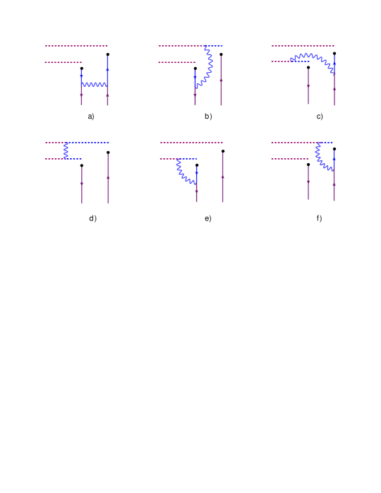
Figure 8: Diagrams with the gauge-dependent part of gluon propagator (denoted by wavy line)

Let us start with the “handbag” diagram in Fig. 8(a). Using standard Ward identities and the equation of motion for background fields ${\bar{\Psi}}\stackrel{{\scriptstyle\leftarrow}}{{\not{P}}}=\not{P}\Psi=0$, we get

$$(y|{1\over\not{P}}|z)\gamma^{\mu}t^{b}\Psi(z)\big{(}\!-i\overleftarrow{D}^{z}_{\mu}\big{)}^{ba}~{}=~{}\delta^{(4)}(z-y)t^{a}\Psi(y),~{}~{}~{}~{}~{}(iD_{\mu}^{z})^{ab}{\bar{\Psi}}(z)t^{b}\gamma^{\mu}(z|{1\over\not{P}}|x)~{}=~{}\delta^{(4)}(z-x){\bar{\Psi}}(x)t^{a}$$ (142)

and therefore the contribution of gauge part of gluon propagator (140) takes the form

$$\langle{\bar{\psi}}(x-{\delta^{\prime}}^{-})\Gamma\psi(y-\delta^{-})\rangle^{\rm gauge}~{}=~{}-ig^{2}\!\int\!dz_{1}dz_{2}\Gamma(y-\delta^{-}|{1\over\not{P}}|z_{1})\gamma^{\mu}t^{a}\Psi(z_{1})(z_{1}|P^{\mu}{1\over P^{4}}P^{\nu}|z_{2})^{ab}{\bar{\Psi}}(z_{2})\gamma_{\nu}t^{b}(z_{2}|{1\over\not{P}}|x-\delta^{-})$$

$$=~{}ig^{2}{\bar{\Psi}}(x-\delta^{-})t^{a}(x|{1\over P^{4}}|y-\delta^{-})t^{a}\Gamma\Psi(y-\delta^{-})~{}\simeq~{}ig^{2}c_{F}{\bar{\Psi}}(x-\delta^{-})(x-\delta^{-}|{1\over p^{4}}|y-\delta^{-})\Gamma\Psi(y-\delta^{-})$$ (143)

where $x=x_{\perp}+x^{+}$, $y=y_{\perp}+y^{+}$, and superscript “gauge” means the contribution of the gauge part of the gluon propagator (140). Next, let us consider diagram in Fig. 8(b). Using Eq. (142) and a similar formula for Wilson lines

$$\!\int_{-\infty}^{y^{+}}\!d{y^{\prime}}^{+}(z|P_{\mu}{1\over P^{4}}P^{-}|{y^{\prime}})^{ab}t~{}=~{}-i\!\int_{-\infty}^{y^{+}}\!\!d{y^{\prime}}^{+}{d\over d{y^{\prime}}^{+}}(z|P_{\mu}{1\over P^{4}}|{y^{\prime}}^{+}+{y^{\prime}}_{\perp})^{ab}=~{}-i(z|P_{\mu}{1\over P^{4}}|y^{+}+y_{\perp})^{ab}$$ (144)

we obtain

$${\bar{\psi}}(x-\delta^{-})[-\infty^{+},y^{+}]_{y}\Gamma\Psi(y-\delta^{-})~{}\stackrel{{\scriptstyle\rm gauge}}{{=}}~{}-g^{2}\!\int\!dz~{}{\bar{\Psi}}(z)\gamma^{\mu}t^{a}(z|{1\over\not{P}}|x-\delta^{-})(z|P_{\mu}{1\over P^{4}}P^{-}|y^{\prime}+y_{\perp})^{ab}t^{b}\Gamma\Psi(y-\delta^{-})$$

$$=~{}-ig^{2}{\bar{\Psi}}(x-\delta^{-})t^{a}t^{b}(x-\delta^{-}|{1\over P^{4}}|y^{\prime}+y_{\perp})^{ab}\Gamma\Psi(y-\delta^{-})~{}\simeq~{}-ig^{2}c_{F}{\bar{\Psi}}(x-\delta^{-})\Gamma\Psi(y-\delta^{-})(x-\delta^{-}|{1\over p^{4}}|y^{\prime}+y_{\perp})$$

(145)

(recall that we use $A^{+}=0$ gauge for background fields). Similarly, for the diagram in Fig. 8(c) we get

$${\bar{\Psi}}(x-\delta^{-})\Gamma[x^{+},-\infty^{+}]_{x}\psi(y-\delta^{-})~{}\stackrel{{\scriptstyle\rm gauge}}{{=}}~{}g^{2}\!\int_{-\infty}^{x^{+}}\!d{x^{\prime}}^{+}{\bar{\Psi}}(x-\delta^{-})\Gamma t^{a}(y-\delta^{-}|{1\over\not{P}}|z)t^{b}\gamma^{\mu}\Psi(z)({x^{\prime}}^{+}+x_{\perp}|P^{-}{1\over P^{4}}P_{\mu}|z)^{ab}$$

$$=~{}-ig^{2}{\bar{\Psi}}(x-\delta^{-})\Gamma t^{a}t^{b}\Psi(y-\delta^{-})(x^{+}+x_{\perp}|{1\over P^{4}}|y-\delta^{-})^{ab}~{}=~{}-ig^{2}c_{F}{\bar{\Psi}}(x-\delta^{-})\Gamma\Psi(y-\delta^{-})(x^{+}+x_{\perp}|{1\over p^{4}}|y-\delta^{-})$$

(146)

where we used Eq. (142) and the formula

$$\!\int_{-\infty}^{x^{+}}\!d{x^{\prime}}^{+}({x^{\prime}}^{+}+x_{\perp}|P^{-}{1\over P^{4}}P_{\mu}|z)^{ab}~{}=~{}i\!\int_{-\infty}^{x^{+}}\!\!d{x^{\prime}}^{+}{d\over d{x^{\prime}}^{+}}({x^{\prime}}^{+}+x_{\perp}|{1\over P^{4}}P_{\mu}|z)^{ab}=~{}i({x}^{+}+x_{\perp}|{1\over P^{4}}P_{\mu}|z)^{ab}$$ (147)

Next, the contribution of the diagram in Fig. 8(d) can be obtained using Eqs. (144) and (147):

$${\bar{\Psi}}(x-\delta^{-})\Gamma[x^{+},-\infty^{+}]_{x}[-\infty^{+},y^{+}]_{y}\Psi(y-\delta^{-})$$ (148)

$$\stackrel{{\scriptstyle\rm gauge}}{{=}}~{}ig^{2}{\bar{\Psi}}(x-\delta^{-})\Gamma t^{a}t^{b}\Psi(y-\delta^{-})\!\int_{-\infty}^{x^{+}}\!d{x^{\prime}}^{+}\!\int_{-\infty}^{y^{+}}\!d{y^{\prime}}^{+}({x^{\prime}}^{+}+x_{\perp}|P^{-}{1\over P^{4}}P^{-}|{y^{\prime}}^{+}+y_{\perp})^{ab}$$

$$=~{}ig^{2}c_{F}{\bar{\Psi}}(x-\delta^{-})\Gamma\Psi(y-\delta^{-})({x}^{+}+x_{\perp}|{1\over p^{4}}|{y}^{+}+y_{\perp})$$ (149)

Finally, let us consider diagrams in Fig. 8(e) and 8(f) . The result for the diagram in Fig. 8(e) can be obtained by taking $x=y$ in Eq. (145):

$${\bar{\psi}}(x-\delta^{-})[x^{+},-\infty^{+}]_{x}\Gamma\Psi(y-\delta^{-})~{}\stackrel{{\scriptstyle\rm gauge}}{{=}}~{}ig^{2}c_{F}{\bar{\Psi}}(x-\delta^{-})\Gamma\Psi(y-\delta^{-})(x^{+}+x_{\perp}-\delta^{-}|{1\over p^{4}}|x^{+}+x_{\perp})$$ (150)

The integral in the RHS is a pure divergence which does not depend on $\delta^{-}$ and should be set to $0$ in the dimensional regularization framework. Similarly, the contribution of the diagram in Fig. 8(f) vanishes.

Thus, the sum of diagrams in Fig. 8 takes the form

$${\bar{\psi}}(x-\delta^{-})\Gamma[x^{+},-\infty^{+}]_{x}[-\infty^{+},y^{+}]_{y}\psi(y-\delta^{-})$$ (151)

$$=~{}ig^{2}c_{F}{\bar{\Psi}}(x-\delta^{-})\Gamma\Psi(y-\delta^{-})\bigg{[}({x}^{+}+x_{\perp}|{1\over p^{4}}|{y}^{+}+y_{\perp})-(x^{+}+x_{\perp}|{1\over p^{4}}|y^{+}+y_{\perp}-\delta^{-})$$

$$-~{}(x^{+}+x_{\perp}-\delta^{-}|{1\over p^{4}}|y^{\prime}+y_{\perp})+(x^{+}+x_{\perp}-\delta^{-}|{1\over p^{4}}|y^{+}+y_{\perp}-\delta^{-})\bigg{]}$$

$$=~{}{g^{2}c_{F}\over 16\pi^{2}}{\bar{\Psi}}(x-\delta^{-})\Gamma\Psi(y-\delta^{-})\Big{[}\ln\Delta_{\perp}^{2}-\ln\big{(}\Delta_{\perp}^{2}-\Delta^{+}\delta^{-}\big{)}-\ln\big{(}\Delta_{\perp}^{2}+\Delta^{+}{\delta^{\prime}}^{-}\big{)}+\ln\big{(}\Delta_{\perp}^{2}+\Delta^{+}({\delta^{\prime}}^{-}-\delta^{-})\big{)}\Big{]}$$

$$=~{}{g^{2}c_{F}\over 16\pi^{2}}{\bar{\Psi}}(x-\delta^{-})\Gamma\Psi(y-\delta^{-})\Big{[}-\ln\Big{(}1-{\Delta^{+}\delta^{-}\over\Delta_{\perp}^{2}}\Big{)}-\ln\Big{(}1+{\Delta^{+}{\delta^{\prime}}^{-}\over\Delta_{\perp}^{2}}\Big{)}+\ln\Big{(}1+{\Delta^{+}({\delta^{\prime}}^{-}-\delta^{-})\over\Delta_{\perp}^{2}}\Big{)}\Big{]}$$

Since ${\Delta^{+}\delta^{-}\over\Delta_{\perp}^{2}}\sim{q_{\perp}^{2}\over\beta_{B}\sigma s}\ll 1$, the sum (151) is a power correction so the leading-order evolution equation (41) is gauge invariant.

Let us discuss now the invariance of the one-loop quark correction. Since the effect of the one-loop correction reduces to replacement ${1\over p^{2}}\rightarrow-{b\alpha_{s}\over 4\pi}{1\over p^{2}}\ln(-p^{2}/\tilde{\mu}^{2})$, the corresponding contribution of “gauge correction diagrams” in Fig. 8 with the extra quark loop is

$$-ig^{2}c_{F}{b\alpha_{s}\over 4\pi}{\bar{\Psi}}(x-\delta^{-})\Gamma\Psi(y-\delta^{-})\bigg{[}({x}^{+}+x_{\perp}|{\ln{-p^{2}\over\tilde{\mu}^{2}}\over p^{4}}|{y}^{+}+y_{\perp})-(x^{+}+x_{\perp}|{\ln{-p^{2}\over\tilde{\mu}^{2}}\over p^{4}}|y^{+}+y_{\perp}-\delta^{-})$$

$$-~{}(x^{+}+x_{\perp}-\delta^{-}|{\ln{-p^{2}\over\tilde{\mu}^{2}}\over p^{4}}|y^{\prime}+y_{\perp})+(x^{+}+x_{\perp}-\delta^{-}|{\ln{-p^{2}\over\tilde{\mu}^{2}}\over p^{4}}|y^{+}+y_{\perp}-\delta^{-})\bigg{]}$$

$$=~{}{g^{2}c_{F}\over 16\pi^{2}}{\bar{\Psi}}(x-\delta^{-})\Gamma\Psi(y-\delta^{-})\Big{[}\ln^{2}\Delta_{\perp}^{2}\tilde{\mu}^{2}-\ln^{2}\big{(}\Delta_{\perp}^{2}-\Delta^{+}\delta^{-}\big{)}\tilde{\mu}^{2}$$

$$-~{}\ln^{2}\big{(}\Delta_{\perp}^{2}+\Delta^{+}{\delta^{\prime}}^{-}\big{)}\tilde{\mu}^{2}+\ln^{2}\big{(}\Delta_{\perp}^{2}+\Delta^{+}({\delta^{\prime}}^{-}-\delta^{-})\big{)}\tilde{\mu}^{2}\Big{]}$$ (152)

which is again a power correction due to ${\Delta^{+}\delta^{-}\over\Delta_{\perp}^{2}}\ll 1$. Consequently, the running-coupling evolution equation (61) is gauge invariant. In a similar way one can prove gauge invariance of the evolution equation of gluon TMD operators.

VII.3 Necessary integrals

In this appendix we calculate some integrals used in the main text. Let us start with the integral

$$16\pi^{2}\!\int\!{{\textstyle d}\lower 0.12915pt\hbox{\kern-3.80005pt${}^{\scriptstyle-}$}\kern-0.50003pt{}p_{\perp}\over p_{\perp}^{2}}\!\int_{0}^{\infty}\!{\textstyle d}\lower 0.12915pt\hbox{\kern-3.80005pt${}^{\scriptstyle-}$}\kern-0.50003pt{}\alpha~{}e^{-i{\alpha\over\sigma}}{\big{(}1-e^{i(p,\Delta)_{\perp}}\big{)}\beta_{B}s\over\alpha\beta_{B}s+(p-p_{B})_{\perp}^{2}+{i\epsilon}}\,.$$ (153)

At $\beta_{B}>0$ we get

$$16\pi^{2}\!\int\!{{\textstyle d}\lower 0.12915pt\hbox{\kern-3.80005pt${}^{\scriptstyle-}$}\kern-0.50003pt{}p_{\perp}\over p_{\perp}^{2}}\!\int_{0}^{\infty}\!{\textstyle d}\lower 0.12915pt\hbox{\kern-3.80005pt${}^{\scriptstyle-}$}\kern-0.50003pt{}\alpha~{}e^{-i{\alpha\over\sigma}}{\big{(}1-e^{i(p,\Delta)_{\perp}}\big{)}\beta_{B}s\over\alpha\beta_{B}s+p_{\perp}^{2}}~{}\stackrel{{\scriptstyle\Lambda\equiv\sigma\beta_{B}s}}{{=}}~{}8\pi\!\int\!{{\textstyle d}\lower 0.12915pt\hbox{\kern-3.80005pt${}^{\scriptstyle-}$}\kern-0.50003pt{}p_{\perp}\over p_{\perp}^{2}}\!\int_{0}^{\infty}\!dt~{}e^{-i{t\over\Lambda}}{\big{(}1-e^{i(p,\Delta)_{\perp}}\big{)}\over t+p_{\perp}^{2}}~{}=~{}$$

$$=~{}2\!\int_{0}^{\infty}\!{dt\over t}e^{-i{t\over\Lambda}}\Big{[}\ln{t\Delta_{\perp}^{2}\over 4}+2\gamma+2K_{0}\big{(}\sqrt{t\Delta_{\perp}^{2}}\big{)}\Big{]}~{}=~{}\ln^{2}\Big{(}-{i\over 4}\sigma\beta_{B}s\Delta_{\perp}^{2}e^{\gamma}\Big{)}+{\pi^{2}\over 2}~{}+~{}O\big{(}{\Delta_{\perp}^{-2}\over\sigma\beta_{B}s}\big{)}$$ (154)

while at $\beta_{B}<0$ we can rotate the contour of integration over $\alpha$ in the lower half-plane of complex $\alpha$ and get

$$16\pi^{2}\!\int\!{{\textstyle d}\lower 0.12915pt\hbox{\kern-3.80005pt${}^{\scriptstyle-}$}\kern-0.50003pt{}p_{\perp}\over p_{\perp}^{2}}\!\int_{0}^{\infty}\!{\textstyle d}\lower 0.12915pt\hbox{\kern-3.80005pt${}^{\scriptstyle-}$}\kern-0.50003pt{}\alpha~{}e^{-i{\alpha\over\sigma}}{\big{(}1-e^{i(p,\Delta)_{\perp}}\big{)}\beta_{B}s\over\alpha\beta_{B}s+p_{\perp}^{2}+{i\epsilon}}~{}=~{}16\pi^{2}\!\int\!{{\textstyle d}\lower 0.12915pt\hbox{\kern-3.80005pt${}^{\scriptstyle-}$}\kern-0.50003pt{}p_{\perp}\over p_{\perp}^{2}}\!\int_{0}^{\infty}\!{\textstyle d}\lower 0.12915pt\hbox{\kern-3.80005pt${}^{\scriptstyle-}$}\kern-0.50003pt{}\alpha~{}e^{i{\alpha\over\sigma}}{\big{(}1-e^{i(p,\Delta)_{\perp}}\big{)}|\beta_{B}|s\over\alpha|\beta_{B}|s+p_{\perp}^{2}}$$

$$=~{}\ln^{2}\Big{(}{i\over 4}\sigma|\beta_{B}|s\Delta_{\perp}^{2}e^{\gamma}\Big{)}+{\pi^{2}\over 2}~{}+~{}O\big{(}{\Delta_{\perp}^{-2}\over\sigma|\beta_{B}|s}\big{)}\,.$$ (155)

The combination of Eqs. (154) and (155) can be written as

$$16\pi^{2}\!\int\!{{\textstyle d}\lower 0.12915pt\hbox{\kern-3.80005pt${}^{\scriptstyle-}$}\kern-0.50003pt{}p_{\perp}\over p_{\perp}^{2}}\!\int_{0}^{\infty}\!{\textstyle d}\lower 0.12915pt\hbox{\kern-3.80005pt${}^{\scriptstyle-}$}\kern-0.50003pt{}\alpha~{}e^{-i{\alpha\over\sigma}}{\big{(}1-e^{i(p,\Delta)_{\perp}}\big{)}\beta_{B}s\over\alpha\beta_{B}s+p_{\perp}^{2}+{i\epsilon}}~{}=~{}\ln^{2}\Big{(}-{i\over 4}(\beta_{B}+{i\epsilon})\sigma s\Delta_{\perp}^{2}e^{\gamma}\Big{)}+{\pi^{2}\over 2}~{}+~{}O\big{(}{m_{\perp}^{2}\over\beta_{B}\sigma s}\big{)}$$ (156)

which reflects the “causal” structure discussed after Eq. (43). From Eq. (30) we get

$$16\pi^{2}\!\int\!{{\textstyle d}\lower 0.12915pt\hbox{\kern-3.80005pt${}^{\scriptstyle-}$}\kern-0.50003pt{}p_{\perp}\over p_{\perp}^{2}}\!\int_{0}^{\infty}\!{\textstyle d}\lower 0.12915pt\hbox{\kern-3.80005pt${}^{\scriptstyle-}$}\kern-0.50003pt{}\alpha~{}e^{-i{\alpha\over\sigma}}{\big{(}1-e^{i(p,\Delta)_{\perp}}\big{)}\beta_{B}s\over\alpha\beta_{B}s+(p-p_{B})_{\perp}^{2}+{i\epsilon}}$$

$$=~{}\ln^{2}\Big{(}-{i\over 4}(\beta_{B}+{i\epsilon})\sigma s\Delta_{\perp}^{2}e^{\gamma}\Big{)}+{\pi^{2}\over 2}-8\pi\!\int\!{{\textstyle d}\lower 0.12915pt\hbox{\kern-3.80005pt${}^{\scriptstyle-}$}\kern-0.50003pt{}p_{\perp}\over p_{\perp}^{2}}\big{(}1-e^{i(p,\Delta)_{\perp}}\big{)}\ln{(p-p_{B})_{\perp}^{2}\over p_{\perp}^{2}}~{}+~{}O\big{(}{m_{\perp}^{2}\over\beta_{B}\sigma s}\big{)}$$ (157)

so

$$\sigma{d\over d\sigma}\!\int_{0}^{\infty}\!{\textstyle d}\lower 0.12915pt\hbox{\kern-3.80005pt${}^{\scriptstyle-}$}\kern-0.50003pt{}\alpha~{}e^{-i{\alpha\over\sigma}}\!\int\!{{\textstyle d}\lower 0.12915pt\hbox{\kern-3.80005pt${}^{\scriptstyle-}$}\kern-0.50003pt{}p_{\perp}\over p_{\perp}^{2}}{\beta_{B}s\big{(}e^{i(p,\Delta)_{\perp}}-1\big{)}\over\alpha(\beta_{B}+{i\epsilon})s+p_{\perp}^{2}}~{}=~{}{\alpha_{s}\over 2\pi}\ln\Big{(}-{i\over 4}(\beta_{B}+{i\epsilon})\sigma s\Delta_{\perp}^{2}e^{\gamma}\Big{)}$$ (158)

Now let us consider the integral with an extra $\ln{\tilde{\mu}^{2}\over p_{\perp}^{2}}$ in Eq. (56),

$$\!\int_{0}^{\infty}\!{{\textstyle d}\lower 0.12915pt\hbox{\kern-3.80005pt${}^{\scriptstyle-}$}\kern-0.50003pt{}\alpha\over\sigma}e^{-i{\alpha\over\sigma}}\!\int\!{\textstyle d}\lower 0.12915pt\hbox{\kern-3.80005pt${}^{\scriptstyle-}$}\kern-0.50003pt{}p_{\perp}{\big{(}e^{i(p,\Delta)_{\perp}}-1\big{)}\alpha\beta_{B}s\ln{\tilde{\mu}^{2}\over p_{\perp}^{2}}\over p_{\perp}^{2}[\alpha\beta_{B}s+p_{\perp}^{2}+{i\epsilon}]}~{}=~{}\!\int_{0}^{\infty}\!{{\textstyle d}\lower 0.12915pt\hbox{\kern-3.80005pt${}^{\scriptstyle-}$}\kern-0.50003pt{}\alpha\over\sigma}e^{-i{\alpha\over\sigma}}\!\int\!{\textstyle d}\lower 0.12915pt\hbox{\kern-3.80005pt${}^{\scriptstyle-}$}\kern-0.50003pt{}p_{\perp}\big{(}e^{i(p,\Delta)_{\perp}}-1\big{)}\Big{[}{1\over p_{\perp}^{2}}-{1\over\alpha\beta_{B}s+p_{\perp}^{2}+{i\epsilon}}\Big{]}\ln{\tilde{\mu}^{2}\over p_{\perp}^{2}}$$

$$=~{}\!\int_{0}^{\infty}\!{{\textstyle d}\lower 0.12915pt\hbox{\kern-3.80005pt${}^{\scriptstyle-}$}\kern-0.50003pt{}\alpha\over\sigma}e^{-i{\alpha\over\sigma}}\!\int\!{\textstyle d}\lower 0.12915pt\hbox{\kern-3.80005pt${}^{\scriptstyle-}$}\kern-0.50003pt{}p_{\perp}\Big{[}{e^{i(p,\Delta)_{\perp}}-1\over p_{\perp}^{2}}+{1\over\alpha\beta_{B}s+p_{\perp}^{2}+{i\epsilon}}\Big{]}\ln{\tilde{\mu}^{2}\over p_{\perp}^{2}}-\!\int_{0}^{\infty}\!{{\textstyle d}\lower 0.12915pt\hbox{\kern-3.80005pt${}^{\scriptstyle-}$}\kern-0.50003pt{}\alpha\over\sigma}e^{-i{\alpha\over\sigma}}\!\int\!{\textstyle d}\lower 0.12915pt\hbox{\kern-3.80005pt${}^{\scriptstyle-}$}\kern-0.50003pt{}p_{\perp}{e^{i(p,\Delta)_{\perp}}\over\alpha\beta_{B}s+p_{\perp}^{2}+{i\epsilon}}\ln{\tilde{\mu}^{2}\over p_{\perp}^{2}}$$ (159)

It is easy to see that the last term in the RHS is actually a power correction:

$$\!\int_{0}^{\infty}\!{{\textstyle d}\lower 0.12915pt\hbox{\kern-3.80005pt${}^{\scriptstyle-}$}\kern-0.50003pt{}\alpha\over\sigma}e^{-i{\alpha\over\sigma}}\!\int\!{\textstyle d}\lower 0.12915pt\hbox{\kern-3.80005pt${}^{\scriptstyle-}$}\kern-0.50003pt{}p_{\perp}{e^{i(p,\Delta)_{\perp}}\over\alpha\beta_{B}s+p_{\perp}^{2}+{i\epsilon}}\ln{\tilde{\mu}^{2}\over p_{\perp}^{2}}~{}=~{}\!\int\!{\textstyle d}\lower 0.12915pt\hbox{\kern-3.80005pt${}^{\scriptstyle-}$}\kern-0.50003pt{}p_{\perp}~{}e^{i(p,\Delta)_{\perp}}\ln{\tilde{\mu}^{2}\over p_{\perp}^{2}}\!\int_{0}^{\infty}\!{{\textstyle d}\lower 0.12915pt\hbox{\kern-3.80005pt${}^{\scriptstyle-}$}\kern-0.50003pt{}\alpha\over\sigma\beta_{B}s}e^{-i{\alpha\over\sigma}}{d\over d\alpha}\ln{\alpha\beta_{B}s+p_{\perp}^{2}+{i\epsilon}\over\tilde{\mu}^{2}}$$

$$\simeq~{}{1\over\sigma\beta_{B}s}\!\int\!{\textstyle d}\lower 0.12915pt\hbox{\kern-3.80005pt${}^{\scriptstyle-}$}\kern-0.50003pt{}p_{\perp}~{}e^{i(p,\Delta)_{\perp}}\ln{p_{\perp}^{2}\over\tilde{\mu}^{2}}\Big{[}{1\over 2\pi}\ln{p_{\perp}^{2}\over\tilde{\mu}^{2}}+i\!\int_{0}^{\sigma}\!{{\textstyle d}\lower 0.12915pt\hbox{\kern-3.80005pt${}^{\scriptstyle-}$}\kern-0.50003pt{}\alpha\over\sigma}\ln{\alpha\beta_{B}s+p_{\perp}^{2}+{i\epsilon}\over\tilde{\mu}^{2}}\Big{]}~{}\sim~{}O\Big{(}{m_{\perp}^{2}\over\sigma\beta_{B}s}\Big{)}$$ (160)

As to the first term in the RHS of Eq. (159), it is easily calculated using standard trick $\big{(}{p^{2}\over\tilde{\mu}^{2}}\big{)}^{\delta}=1+\delta\ln{p^{2}\over\tilde{\mu}^{2}}+O(\delta^{2})$

$$\!\int_{0}^{\infty}\!{{\textstyle d}\lower 0.12915pt\hbox{\kern-3.80005pt${}^{\scriptstyle-}$}\kern-0.50003pt{}\alpha\over\sigma}e^{-i{\alpha\over\sigma}}\!\int\!{\textstyle d}\lower 0.12915pt\hbox{\kern-3.80005pt${}^{\scriptstyle-}$}\kern-0.50003pt{}p_{\perp}\Big{[}{e^{i(p,\Delta)_{\perp}}-1\over p_{\perp}^{2}}+{1\over\alpha\beta_{B}s+p_{\perp}^{2}+{i\epsilon}}\Big{]}\ln{\tilde{\mu}^{2}\over p_{\perp}^{2}}$$

$$=~{}{i\over 16\pi^{2}}\Big{[}\big{(}\ln{\Delta_{\perp}^{2}\tilde{\mu}^{2}\over 4}+2\gamma\big{)}^{2}-\big{(}\ln{-i\sigma(\beta_{B}+{i\epsilon})s\over\tilde{\mu}^{2}}-\gamma\big{)}^{2}-{\pi^{2}\over 2}\Big{]}$$

$$=~{}{i\over 16\pi^{2}}\Big{[}\big{(}\ln{\Delta_{\perp}^{2}\over 4}[-i\sigma(\beta_{B}+{i\epsilon})s]+\gamma\big{)}\big{(}\ln{\Delta_{\perp}^{2}\tilde{\mu}^{4}/4\over-i\sigma(\beta_{B}+{i\epsilon})s}+3\gamma\big{)}-{\pi^{2}\over 2}\Big{]}$$ (161)

This gives us Eq. (59).

VII.4 The light-cone expansion of propagators

In this appendix we derive the light-cone expansion of various propagators in the first order in the background field with one (quark) loop accuracy. First, we present necessary formulas for quark propagators. The typical integral appears as

$$(x|{\Gamma(a)\over(-p^{2}-{i\epsilon})^{a}}\Phi{\Gamma(b)\over(-p^{2}-{i\epsilon})^{b}}|0)~{}=~{}i^{a+b}\int_{0}^{\infty}\!ds~{}s^{a+b-1}\!\int_{0}^{1}\!du~{}{\bar{u}}^{a-1}u^{b-1}(x|e^{is{\bar{u}}p^{2}}\Phi e^{isup^{2}}|0)$$ (162)

where $\Phi(z)$ is some operator, such as $\Psi(z)$ or ${\cal F}_{\mu\nu}(z)$. Using expansion in powers of proper time $s$ Balitsky:1987bk ,

$$(x|e^{is{\bar{u}}p^{2}}\Phi e^{isup^{2}}|0)~{}=~{}(x|e^{isp^{2}}|0)\Big{[}\!\int_{0}^{1}\!du~{}\Phi(ux)-is\!\int_{0}^{1}\!du~{}{\bar{u}}u\partial^{2}\Phi(ux)~{}+~{}O(s^{2})\Big{]}$$ (163)

we get the light-cone expansion

$$(x|{\Gamma(a)\over(-p^{2})^{a}}\Phi{\Gamma(b)\over(-p^{2})^{b}}|0)~{}=~{}(x|{\Gamma(a+b)\over(-p^{2})^{a+b}}|0)\!\int_{0}^{1}\!du~{}{\bar{u}}^{a-1}u^{b-1}\Phi(ux)-(x|{\Gamma(a+b+1)\over(-p^{2})^{a+b+1}}|0)\!\int_{0}^{1}\!du~{}{\bar{u}}^{a}u^{b}\partial^{2}\Phi(ux)~{}+~{}...$$ (164)

For our background fields that depend only on $x^{+}$ we need only the first term of this expansion since $\partial^{2}\Phi(x^{+})=0$ so

$$(x|{\Gamma(a)\over(-p^{2})^{a}}\Phi{\Gamma(b)\over(-p^{2})^{b}}|0)~{}=~{}(x|{\Gamma(a+b)\over(-p^{2})^{a+b}}|0)\!\int_{0}^{1}\!du~{}{\bar{u}}^{a-1}u^{b-1}\Phi(ux)$$ (165)

This is our master formula for light-cone expansions. In this appendix we discuss only Feynman propagators so $p^{2}$ always means $p^{2}+{i\epsilon}$.

Let us start from the light-cone expansion of Eq. (67). Using standard trick

$$(x|{\ln{\tilde{\mu}^{2}\over-p^{2}}\over p^{2}}\Phi{1\over p^{2}}|0)~{}=~{}\bigg{[}(x|{\tilde{\mu}^{2\lambda}\over(-p^{2})^{1+\lambda}}\Phi{1\over(-p^{2})}|0)\bigg{]}_{\lambda}$$ (166)

where $\big{[}\dots\big{]}_{\lambda}$ denotes the first nontrivial term in the expansion in powers of $\lambda$, we obtain

$$(x|{\ln{\tilde{\mu}^{2}\over-p^{2}}\over p^{2}}\Phi{1\over p^{2}}|0)~{}=~{}(x|{\ln{\tilde{\mu}^{2}\over-p^{2}}\over p^{4}}|0)\!\int_{0}^{1}\!du~{}\Phi(ux)+(x|{1\over p^{4}}|0)\!\int_{0}^{1}\!du~{}(1+\ln{\bar{u}})\Phi(ux)$$

$$=~{}{i\Gamma\big{(}{\varepsilon})\over 16\pi^{d\over 2}(-x^{2})^{\varepsilon}}\Big{(}\big{[}\ln{-\tilde{\mu}^{2}x^{2}\over 4}+{1\over{\varepsilon}}-\psi(1+{\varepsilon})+\gamma\big{]}\!\int_{0}^{1}\!du~{}\Phi(ux)+\!\int_{0}^{1}\!du~{}\ln{\bar{u}}\Phi(ux)\Big{)}$$ (167)

where we used Eq. (165).

Restoring the end point $y$ we obtain

$$(x|{1\over p^{2}}\Phi{\ln{\tilde{\mu}^{2}\over-p^{2}}\over p^{2}}|y)~{}=~{}(x|{\ln{\tilde{\mu}^{2}\over-p^{2}}\over p^{4}}|y)\!\int_{0}^{1}\!du~{}\Phi(x_{u})+(x|{1\over p^{4}}|y)\!\int_{0}^{1}\!du~{}(1+\ln u)\Phi(x_{u})$$

$$(x|{\ln{\tilde{\mu}^{2}\over-p^{2}}\over p^{2}}\Phi{1\over p^{2}}|y)~{}=~{}(x|{\ln{\tilde{\mu}^{2}\over-p^{2}}\over p^{4}}|y)\!\int_{0}^{1}\!du~{}\Phi(x_{u})+(x|{1\over p^{4}}|y)\!\int_{0}^{1}\!du~{}(1+\ln{\bar{u}})\Phi(x_{u})$$ (168)

where $x_{u}=ux+{\bar{u}}y$ as usual.

We will also need formulas for differentiation with respect to the point-splitting cutoff. The master formula is

$$-\delta^{-}{d\over d\delta^{-}}\!\int_{-\infty}^{0}\!dz^{+}~{}f(x_{\perp}^{2}-2z^{+}\delta^{-})\!\int_{0}^{t}\!du~{}\Phi(uz^{+})~{}\stackrel{{\scriptstyle 1>t>0}}{{=}}~{}\int_{-\infty}^{0}\!dz^{+}\Phi(z^{+})f\big{(}x_{\perp}^{2}-{2\over t}z^{+}\delta^{-}\big{)}$$ (169)

and corollaries

$$\delta^{-}{d\over d\delta^{-}}\!\int_{-\infty}^{0}\!dz^{+}~{}f(x_{\perp}^{2}-2z^{+}\delta^{-})\!\int_{0}^{1}\!du~{}\ln u~{}\Phi(uz^{+})~{}=~{}\int_{-\infty}^{0}\!dz^{+}\Phi(z^{+})\int_{0}^{1}\!{dt\over t}~{}f\big{(}x_{\perp}^{2}-{2\over t}z^{+}\delta^{-}\big{)}$$ (170)

$$\delta^{-}{d\over d\delta^{-}}\!\int_{-\infty}^{0}\!dz^{+}~{}f(x_{\perp}^{2}-2z^{+}\delta^{-})\!\int_{0}^{1}\!du~{}\ln{\bar{u}}~{}\Phi(uz^{+})~{}=~{}\int_{-\infty}^{0}\!dz^{+}\Phi(z^{+})\int_{0}^{1}\!{dt\over 1-t}~{}\Big{[}f\big{(}x_{\perp}^{2}-2z^{+}\delta^{-}\big{)}-f\big{(}x_{\perp}^{2}-{2\over t}z^{+}\delta^{-}\big{)}\Big{]}$$

Next, let us present formulas relevant for the gluon propagator (109) (see Fig. 7):

$$\langle A^{a}_{\mu}(x)A^{b}_{\nu}(y)\rangle_{\rm quark~{}loop}~{}=~{}{g^{2}\over 24\pi^{2}}\Big{\{}ig_{\mu\nu}(x|{\ln-\tilde{\mu}^{2}/P^{2}\over P^{2}}|y)-i(x|P_{\mu}{\ln-\tilde{\mu}^{2}/P^{2}\over P^{4}}P_{\nu}|y)+2(x|{1\over p^{2}}\big{\{}{\cal F}_{\mu\nu},\ln{\tilde{\mu}^{2}\over-p^{2}}\big{\}}{1\over p^{2}}|y)$$

$$\hskip 14.22636pt-~{}\!\int\!dz_{1}dz_{2}\!\int_{0}^{1}\!du~{}\Big{[}u(x|{1\over p^{2}}]z_{1}){\cal F}_{\mu\xi}(z_{u})(z_{1}|{p^{\xi}\over p^{2}}|z_{2})(z_{2}|{p_{\nu}\over p^{2}}|y)-{\bar{u}}(x|{p_{\mu}\over p^{2}}]z_{1}){\cal F}_{\nu\xi}(z_{u})(z_{1}|{p^{\xi}\over p^{2}}|z_{2})(z_{2}|{1\over p^{2}}|y)$$

$$\hskip 28.45274pt-~{}(x|{1\over p^{2}}|z_{1})\Big{(}2i{\bar{u}}u(z_{1}|{p^{\xi}\over p^{2}}|z_{2})(D_{\mu}{\cal F}_{\nu\xi}(z_{u})+\mu\leftrightarrow\nu)+(z_{1}|2\ln{\tilde{\mu}^{2}\over-p^{2}}-{5\over 2}|z_{2}){\cal F}_{\mu\nu}(z_{u})\Big{)}(z_{2}|{1\over p^{2}}|y)\Big{]}\Big{\}}$$ (171)

To get the light-cone expansion of the gluon propagator we need a formula

$$(x|e^{isP^{2}}|y)~{}=~{}(x|e^{isp^{2}}|y)\Big{(}[x,y]+s\!\int_{0}^{1}\!du~{}{\bar{u}}u[x,x_{u}]D^{\mu}{\cal F}_{\mu x}(x_{u})[x_{u},y]$$

$$+~{}2i\!\int_{0}^{1}\!du\!\int_{0}^{u}\!dv~{}{\bar{u}}v[x,x_{u}]{\cal F}_{\mu x}(x_{u})[x_{u},x_{v}]{\cal F}^{\mu}_{~{}x}(x_{v})[vx,y]~{}+~{}O(s^{2})\Big{)}~{}=~{}(x|e^{isp^{2}}|y)[x,y]~{}+~{}O(D{\cal F},{\cal F}^{2})$$ (172)

(where ${\cal F}_{\mu x}\equiv x^{\xi}{\cal F}_{\mu\xi}$) and therefore

$$(x|f(P^{2})|y)~{}=~{}[x,y](x|f(p^{2})|y)$$ (173)

in our approximation. Hereafter $+~{}O(D{\cal F},{\cal F}^{2})$ is assumed in all equations. By differentiation of gauge link $[x,y]$ using formulas

$$i{\partial\over\partial x_{\mu}}[ux+{\bar{u}}y,vx+{\bar{v}}y]~{}=~{}-uA_{\mu}(x_{u})[x_{u},x_{v}]+[x_{u},x_{v}]vA_{\mu}(x_{v})+\!\int_{v}^{u}\!dt~{}t[x_{u},x_{t}]{\cal F}_{x\mu}(x_{t})[x_{t},x_{v}]$$

$$[ux+{\bar{u}}y,vx+{\bar{v}}y]\big{(}-i\stackrel{{\scriptstyle\leftarrow}}{{\partial\over\partial y_{\nu}}}\big{)}~{}=~{}{\bar{u}}A_{\nu}(x_{u})[x_{u},x_{v}]-[x_{u},x_{v}]{\bar{v}}A_{\nu}(x_{v})-\!\int_{v}^{u}\!dt~{}{\bar{t}}[x_{u},x_{t}]{\cal F}_{x\nu}(x_{t})[x_{t},x_{v}]$$ (174)

(where $x_{t}=tx+{\bar{t}}y$ as usual) one obtains

$$(x|g_{\mu\nu}{\Gamma(a)\over(-P^{2})^{a-1}}+P_{\mu}{\Gamma(a)\over(-P^{2})^{a}}P_{\nu}|y)~{}=~{}~{}[x,y](x|g_{\mu\nu}{\Gamma(a)\over(-p^{2})^{a-1}}+p_{\mu}{\Gamma(a)\over(-p^{2})^{a}}p_{\nu}|y)$$

$$+~{}\!\int_{0}^{1}\!du~{}\Big{(}u[x,x_{u}]{\cal F}_{x\mu}(x_{u})[x_{u},y](x|{p_{\nu}\Gamma(a)\over(-p^{2})^{a}}|y)-{\bar{u}}[x,x_{u}]{\cal F}_{x\nu}(x_{u})[x_{u},y](x|{p_{\mu}\Gamma(a)\over(-p^{2})^{a}}|y)$$

$$-~{}{i\over 2}(x|{\Gamma(a)\over(-p^{2})^{a}}|y)\!\int_{0}^{1}\!du~{}[x,x_{u}]\Big{(}{\cal F}_{\mu\nu}(x_{u})-{\bar{u}}u(D_{\mu}{\cal F}_{\nu x}(x_{u})+\mu\leftrightarrow\nu)\Big{)}[x_{u},y]~{}+~{}O(D{\cal F},{\cal F}^{2})$$

$$\hskip 14.22636pt=~{}[x,y](x|(p_{\mu}p_{\nu}-p^{2}g_{\mu\nu}){\Gamma(a)\over(-p^{2})^{a}}|y)-{2\Gamma\big{(}{d\over 2}-a+1\big{)}\over 4^{a}\pi^{d\over 2}(-\Delta^{2})^{{d\over 2}-a+1}}\!\int_{0}^{1}\!du~{}[x,x_{u}]\big{(}u\Delta_{\nu}{\cal F}_{\Delta\mu}(x_{u})-{\bar{u}}\Delta_{\mu}{\cal F}_{\Delta\nu}(x_{u})\big{)}[x_{u},y]$$

$$\hskip 31.29802pt+~{}{\Gamma\big{(}{d\over 2}-a\big{)}\over 4^{a}\pi^{d\over 2}(-\Delta^{2})^{{d\over 2}-a}}{1\over 2}\!\int_{0}^{1}\!du[x,x_{u}]\big{(}{\cal F}_{\mu\nu}(x_{u})-{\bar{u}}u(D_{\mu}{\cal F}_{\nu\Delta}(x_{u})+\mu\leftrightarrow\nu)\big{)}[x_{u},y]~{}+~{}O(D{\cal F},{\cal F}^{2})$$ (175)

where $\Delta\equiv x-y$. Using this formula it is easy to get the first term in Eq. (171),

$$ig_{\mu\nu}(x|{\ln-\tilde{\mu}^{2}/P^{2}\over P^{2}}|y)-i(x|P_{\mu}{\ln-\tilde{\mu}^{2}/P^{2}\over P^{4}}P_{\nu}|0)~{}=~{}i(x|g_{\mu\nu}{\ln-\tilde{\mu}^{2}/p^{2}\over p^{2}}-p_{\mu}p_{\nu}{\ln-\tilde{\mu}^{2}/p^{2}\over p^{4}}|y)$$

$$+~{}{i\over 8\pi^{2+{\varepsilon}}}{\Gamma(1+{\varepsilon})\over(-\Delta^{2})^{1+{\varepsilon}}}\big{[}\ln{-\tilde{\mu}^{2}\Delta^{2}\over 4}-\psi(1+{\varepsilon})-\psi(2)\big{]}\!\int_{0}^{1}\!du~{}\big{(}u\Delta_{\nu}{\cal F}_{\Delta\mu}(x_{u})-{\bar{u}}\Delta_{\mu}{\cal F}_{\Delta\nu}(x_{u})\big{)}$$

$$-~{}{i\Gamma\big{(}{\varepsilon})\over 32\pi^{d\over 2}(-\Delta^{2})^{\varepsilon}}\Big{[}{1\over{\varepsilon}}+\ln{-\tilde{\mu}^{2}\Delta^{2}\over 4}-\psi(1+{\varepsilon})-\psi(2)\Big{]}\!\int_{0}^{1}\!du~{}\big{(}{\cal F}_{\mu\nu}(x_{u})-{\bar{u}}u(D_{\mu}{\cal F}_{\nu\Delta}(x_{u})+\mu\leftrightarrow\nu)\big{)}$$ (176)

Hereafter we drop gauge links for brevity.

The last term in the first line of Eq. (171) follows easily from Eq. (168):

$$(x|{1\over p^{2}}\big{\{}{\cal F}_{\mu\nu},\ln{\tilde{\mu}^{2}\over-p^{2}}\big{\}}{1\over p^{2}}|y)~{}=~{}2(x|{\ln{\tilde{\mu}^{2}\over-p^{2}}\over p^{4}}|y)\!\int_{0}^{1}\!du~{}{\cal F}_{\mu\nu}(x_{u})+(x|{1\over p^{4}}|y)\!\int_{0}^{1}\!du~{}(2+\ln{\bar{u}}u){\cal F}_{\mu\nu}(x_{u})$$

$$=~{}{i\Gamma\big{(}{\varepsilon})\over 8\pi^{d\over 2}(-\Delta^{2})^{\varepsilon}}\Big{(}\big{[}\ln{-\tilde{\mu}^{2}\Delta^{2}\over 4}+{1\over{\varepsilon}}-\psi(1+{\varepsilon})+\gamma\big{]}\!\int_{0}^{1}\!du~{}{\cal F}_{\mu\nu}(x_{u})+{1\over 2}\!\int_{0}^{1}\!du~{}\ln{\bar{u}}u~{}{\cal F}_{\mu\nu}(x_{u})\Big{)}$$ (177)

To calculate terms in the second and third lines of Eq. (171) we use formulas

$$(x|{1\over p^{2}}|z_{1})(z_{1}|{\Gamma(a)\over(-p^{2})^{a}}|z_{2})\!\int_{0}^{1}\!du~{}{\cal F}_{\alpha\beta}(uz_{1}+{\bar{u}}z_{2})(z_{2}|{1\over p^{2}}|y)=~{}-i^{a}\!\int_{0}^{\infty}\!ds_{1}ds_{2}\!\int_{0}^{s_{1}}\!\int_{0}^{s_{2}}{dt_{1}dt_{2}\over(t_{1}+t_{2})^{2-a}}$$

$$\hskip 31.29802pt\times~{}(x|e^{is_{1}p^{2}}{\cal F}_{\alpha\beta}e^{is_{2}p^{2}}p_{\beta}|y)~{}=~{}-{i^{a}\over a(a-1)}\!\int_{0}^{\infty}\!ds_{1}ds_{2}\big{[}(s_{1}+s_{2})^{a}-s_{1}^{a}-s_{2}^{a}\big{]}(x|e^{is_{1}p^{2}}{\cal F}_{\alpha\xi}e^{is_{2}p^{2}}p_{\beta}|y)$$

$$\hskip 62.59605pt=~{}{1\over a(a-1)}(x|{\Gamma(a+2)\over(-p^{2})^{a+2}}|y)\!\int_{0}^{1}\!du\big{[}1-{\bar{u}}^{a}-u^{a}\big{]}{\cal F}_{\alpha\beta}(ux+{\bar{u}}y)$$ (178)

and

$$(x|{p^{\xi}\over p^{2}}|z_{1})(z_{1}|{\Gamma(a)\over(-p^{2})^{a}}|z_{2})\!\int_{0}^{1}\!du~{}u{\cal F}_{\alpha\xi}(uz_{1}+{\bar{u}}z_{2})(z_{2}|{p_{\beta}\over p^{2}}|y)$$ (179)

$$=~{}-i^{a}\!\int_{0}^{\infty}\!ds_{1}ds_{2}\!\int_{0}^{s_{1}}\!\int_{0}^{s_{2}}{t_{2}dt_{1}dt_{2}\over(t_{1}+t_{2})^{3-a}}(x|p^{\xi}e^{is_{1}p^{2}}{\cal F}_{\alpha\xi}e^{is_{2}p^{2}}p_{\beta}|y)$$

$$=~{}{i^{a}\over a(a-1)(a-2)}\!\int_{0}^{\infty}\!ds_{1}ds_{2}\big{[}(s_{1}+s_{2})^{a}-as_{2}(s_{1}+s_{2})^{a-1}-s_{1}^{a}-s_{2}^{a}+as_{2}^{a}\big{]}(x|p^{\xi}e^{is_{1}p^{2}}{\cal F}_{\alpha\xi}e^{is_{2}p^{2}}p_{\beta}|y)$$

$$=~{}{1\over a(2-a)}\!\int_{0}^{1}\!du\Big{[}-u+u^{a}+{\bar{u}}{1-{\bar{u}}^{a-1}\over a-1}\Big{]}\Big{[}{\cal F}_{\alpha\xi}(ux+{\bar{u}}y)(x|{\Gamma(a+2)p^{\xi}p_{\beta}\over(-p^{2})^{a+2}}|y)-i{\bar{u}}D_{\beta}{\cal F}_{\alpha\xi}(ux+{\bar{u}}y)(x|{\Gamma(a+2)p^{\xi}\over(-p^{2})^{a+2}}|y)\Big{]}$$

where we neglected $D^{\xi}{\cal F}_{\alpha\xi}$ as usual. Similarly

$$(x|{p_{\alpha}\over p^{2}}|z_{1})(z_{1}|{\Gamma(a)\over(-p^{2})^{a}}|z_{2})\!\int_{0}^{1}\!du~{}{\bar{u}}{\cal F}_{\beta\xi}(uz_{1}+{\bar{u}}z_{2})(z_{2}|{p^{\xi}\over p^{2}}|y)$$ (180)

$$=~{}{1\over a(2-a)}\!\int_{0}^{1}\!du\big{[}-{\bar{u}}+{\bar{u}}^{a}+u{1-u^{a-1}\over a-1}\big{]}\Big{[}{\cal F}_{\beta\xi}(ux+{\bar{u}}y)(x|{p_{\alpha}p^{\xi}\Gamma(a+2)\over(-p^{2})^{a+2}}|y)+iuD_{\alpha}{\cal F}_{\beta\xi}(ux+{\bar{u}}y)(x|{p^{\xi}\Gamma(a+2)\over(-p^{2})^{a+2}}|y)\Big{]}$$

and

$$(x|{1\over p^{2}}|z_{1})(z_{1}|{p^{\xi}\Gamma(a)\over(-p^{2})^{a}}|z_{2})\!\int_{0}^{1}\!du~{}{\bar{u}}uD_{\alpha}{\cal F}_{\beta\xi}(uz_{1}+{\bar{u}}z_{2})(z_{2}|{1\over p^{2}}|y)$$

$$=~{}-{1\over a(2-a)(3-a)}(x|{p^{\xi}\Gamma(a+2)\over(-p^{2})^{a+2}}|y)\!\int_{0}^{1}\!du\big{[}1-{\bar{u}}^{a}-u^{a}-a{\bar{u}}u\big{]}D_{\alpha}{\cal F}_{\beta\xi}(ux+{\bar{u}}y)$$ (181)

Using the above formulas, we obtain

$$-\!\int\!dz_{1}dz_{2}\!\int_{0}^{1}\!du~{}\Big{[}u(x|{1\over p^{2}}]z_{1}){\cal F}_{\mu\xi}(z_{u})(z_{1}|{p^{\xi}\over p^{2}}|z_{2})(z_{2}|{p_{\nu}\over p^{2}}|y)-{\bar{u}}(x|{p_{\mu}\over p^{2}}]z_{1}){\cal F}_{\nu\xi}(z_{u})(z_{1}|{p^{\xi}\over p^{2}}|z_{2})(z_{2}|{1\over p^{2}}|y)$$

$$\hskip 28.45274pt+2i{\bar{u}}u(z_{1}|{p^{\xi}\over p^{2}}|z_{2})(D_{\mu}{\cal F}_{\nu\xi}(z_{u})+\mu\leftrightarrow\nu)\Big{)}(z_{2}|{1\over p^{2}}|y)\Big{]}\Big{\}}$$

$$=~{}-{i\over 16\pi^{2}\Delta^{2}}\!\int_{0}^{1}\!du~{}\big{[}{\bar{u}}\ln{\bar{u}}~{}\Delta_{\nu}{\cal F}_{\mu\Delta}(x_{u})-u\ln u~{}\Delta_{\mu}{\cal F}_{\nu\Delta}(x_{u}))\big{]}+{i\over 32\pi^{d\over 2}}{\Gamma({\varepsilon})\over(-\Delta^{2})^{{\varepsilon}}}\!\int_{0}^{1}\!du~{}(u\ln u+{\bar{u}}\ln{\bar{u}}){\cal F}_{\mu\nu}(x_{u})$$

$$-~{}{i\over 32\pi^{d\over 2}}{\Gamma({\varepsilon})\over(-\Delta^{2})^{{\varepsilon}}}\!\int_{0}^{1}\!du~{}\big{[}u^{2}\ln uD_{\mu}{\cal F}_{\nu\Delta}(x_{u})+{\bar{u}}^{2}\ln{\bar{u}}D_{\nu}{\cal F}_{\mu\Delta}(x_{u})+{\bar{u}}u\big{(}D_{\mu}{\cal F}_{\nu\Delta}(x_{u})+\mu\leftrightarrow\nu\big{)}\big{]}$$ (182)

and

$$\!\int\!dz_{1}dz_{2}\!\int_{0}^{1}\!du~{}(x|{1\over p^{2}}|z_{1})(z_{1}|2\ln{\tilde{\mu}^{2}\over-p^{2}}-{5\over 2}|z_{2}){\cal F}_{\mu\nu}(z_{u})(z_{2}|{1\over p^{2}}|y)$$

$$\hskip 31.29802pt=~{}{i\Gamma\big{(}{\varepsilon})\over 8\pi^{d\over 2}(-\Delta^{2})^{\varepsilon}}\Big{(}\big{[}\ln{-\tilde{\mu}^{2}\Delta^{2}\over 4}+{1\over{\varepsilon}}-\psi(1+{\varepsilon})+\gamma-{5\over 4}\big{]}\!\int_{0}^{1}\!du~{}{\cal F}_{\mu\nu}(x_{u})+\!\int_{0}^{1}\!du~{}\ln{\bar{u}}u~{}{\cal F}_{\mu\nu}(x_{u})\Big{)}$$ (183)

Let us present the final formula for the one-loop correction to the gluon propagator in the background field (${\varepsilon}={d\over 2}-2$):

$$\langle A^{a}_{\mu}(x)A^{b}_{\nu}(y)\rangle_{\rm quark~{}loop}^{ab}~{}=~{}{g^{2}\over 24\pi^{2}}\bigg{\{}i(x|g_{\mu\nu}{\ln-\tilde{\mu}^{2}/p^{2}\over p^{2}}-p_{\mu}p_{\nu}{\ln-\tilde{\mu}^{2}/p^{2}\over p^{4}}|y)$$

$$+~{}{i\over 8\pi^{2}}{1\over\Delta^{2}}\big{[}\ln{-\tilde{\mu}^{2}\Delta^{2}\over 4}-1+2\gamma\big{]}\!\int_{0}^{1}\!du~{}\big{(}u\Delta_{\nu}{\cal F}_{\mu\Delta}(x_{u})-{\bar{u}}\Delta_{\mu}{\cal F}_{\nu\Delta}(x_{u})\big{)}$$

$$-~{}{i\over 16\pi^{2}\Delta^{2}}\!\int_{0}^{1}\!du~{}\big{[}{\bar{u}}\ln{\bar{u}}~{}\Delta_{\nu}{\cal F}_{\mu\Delta}(x_{u})-u\ln u~{}\Delta_{\mu}{\cal F}_{\nu\Delta}(x_{u}))\big{]}$$

$$+~{}{i\Gamma\big{(}{\varepsilon})\over 32\pi^{d\over 2}(-\Delta^{2})^{\varepsilon}}\!\int_{0}^{1}\!du~{}{\cal F}_{\mu\nu}(x_{u})\Big{(}-{1\over{\varepsilon}}-\ln{-\tilde{\mu}^{2}\Delta^{2}\over 4}+\psi(1+{\varepsilon})-\gamma+6-4\ln{\bar{u}}u+u\ln u+{\bar{u}}\ln{\bar{u}}\Big{)}$$

$$+~{}{i\Gamma\big{(}{\varepsilon})\over 32\pi^{d\over 2}(-\Delta^{2})^{\varepsilon}}\Big{[}{1\over{\varepsilon}}+\ln{-\tilde{\mu}^{2}\Delta^{2}\over 4}-\psi(1+{\varepsilon})-2+\gamma\Big{]}\!\int_{0}^{1}\!du~{}{\bar{u}}u(D_{\mu}{\cal F}_{\nu\Delta}(x_{u})+\mu\leftrightarrow\nu)$$

$$-~{}{i\over 32\pi^{d\over 2}}{\Gamma({\varepsilon})\over(-\Delta^{2})^{{\varepsilon}}}\!\int_{0}^{1}\!du~{}\big{[}u^{2}\ln uD_{\mu}{\cal F}_{\nu\Delta}(x_{u})+{\bar{u}}^{2}\ln{\bar{u}}D_{\nu}{\cal F}_{\mu\Delta}(x_{u})\big{]}\bigg{\}}^{ab}~{}+~{}O\big{(}D^{\mu}{\cal F}_{\mu\nu},{\cal F}_{\mu\nu}{\cal F}^{\alpha\beta}\big{)}$$ (184)

As usual, the lightlike gauge links are implied.

VII.5 Formulas for the light-cone expansions in Sect. V.2

In principle, we can use Eq. (184) to find e.g. Eq. (112), but calculations are greatly simplified by using some intermediate results such as Eq. (110) since many of the terms in Eq. (184) cancel after differentiation. To use Eq. (110), we need some additional formulas listed here.

First, similar to Eq. (180) one obtains

$$\!\int\!dz_{1}dz_{2}\!\int_{0}^{1}\!du~{}{\bar{u}}(x|{1\over p^{2}}]z_{1}){\cal F}_{\nu\xi}(z_{u})(z_{1}|{p^{\xi}\over p^{2}}|z_{2})(z_{2}|{p_{\mu}\over p^{2}}|y)~{}-~{}(\mu\leftrightarrow\nu)=~{}{i\Delta_{\mu}\over 16\pi^{d\over 2}\Delta^{2}}\!\int_{0}^{1}\!du~{}u\ln u~{}{\cal F}_{\nu\Delta}(x_{u})$$

$$+~{}{i\over 32\pi^{d\over 2}}{\Gamma({\varepsilon})\over(-\Delta^{2})^{{\varepsilon}}}\!\int_{0}^{1}\!du~{}u\ln u~{}{\cal F}_{\mu\nu}(x_{u})+{i\over 32\pi^{d\over 2}}{\Gamma({\varepsilon})\over(-\Delta^{2})^{{\varepsilon}}}\!\int_{0}^{1}\!du~{}{\bar{u}}u\ln u~{}D_{\mu}{\cal F}_{\nu\Delta}(x_{u})~{}-~{}(\mu\leftrightarrow\nu)$$

$$=~{}{i\Delta_{\mu}\over 16\pi^{d\over 2}\Delta^{2}}\!\int_{0}^{1}\!du~{}u\ln u~{}{\cal F}_{\nu\Delta}(x_{u})~{}-~{}(\mu\leftrightarrow\nu)+~{}{i\over 32\pi^{d\over 2}}{\Gamma({\varepsilon})\over(-\Delta^{2})^{{\varepsilon}}}\!\int_{0}^{1}\!du~{}(\ln u+{\bar{u}}u)~{}{\cal F}_{\mu\nu}(x_{u})$$ (185)

Second, we need formulas

$$\delta^{-}{d\over d\delta^{-}}\!\int_{-\infty}^{0}\!dz^{+}~{}{\Gamma(a)\over(x_{\perp}^{2}-2z^{+}\delta^{-}\big{)}^{a}}\!\int_{0}^{1}\!du~{}{\bar{u}}~{}{\cal O}(uz^{+})~{}=~{}-\int_{0}^{1}\!du\!\int_{-\infty}^{0}\!dz^{+}{\cal O}(z^{+}){\Gamma(a)\over(x_{\perp}^{2}-{2\over u}z^{+}\delta^{-})^{a}}$$

$$\delta^{-}{d\over d\delta^{-}}\!\int_{-\infty}^{0}\!dz^{+}~{}{\Gamma(a)\over(x_{\perp}^{2}-2z^{+}\delta^{-}\big{)}^{a}}\!\int_{0}^{1}\!du~{}{\bar{u}}u~{}{\cal O}(uz^{+})~{}=~{}\int_{0}^{1}\!dt~{}(1-2t)\!\int_{-\infty}^{0}\!dz^{+}{\cal O}(z^{+}){\Gamma(a)\over(x_{\perp}^{2}-{2\over t}z^{+}\delta^{-})^{a}}$$

$$=~{}\!\int_{-\infty}^{0}\!dz^{+}{\cal O}(z^{+})\!\int_{0}^{1}\!du~{}{{\bar{u}}\over u}{2z^{+}\delta^{-}\Gamma(a+1)\over(x_{\perp}^{2}-{2\over u}z^{+}\delta^{-})^{a+1}}$$ (186)

which follow from Eq. (169), and

$$\!\int\!dz_{1}dz_{2}\!\int_{0}^{1}\!du~{}(x|{1\over p^{2}}|z_{1})(z_{1}|{p^{j}\over p^{2}}|z_{2})\!\int_{0}^{1}\!du~{}{\bar{u}}uD^{-}{\cal F}^{-,j}(uz_{1}+{\bar{u}}z_{2})(z_{2}|{p_{i}\over p^{2}}|y)$$

$$=~{}(x|{p_{i}p_{j}\over(p^{2})^{3}}|y)\!\int_{0}^{1}\!du~{}{\bar{u}}uD^{-}{\cal F}^{-,j}(ux+{\bar{u}}y)=~{}i\!\int_{0}^{1}\!du~{}{\bar{u}}u~{}D^{-}{\cal F}^{-,j}(ux+{\bar{u}}y)\Big{(}{g_{ij}\Gamma({\varepsilon})\over 64\pi^{d\over 2}(-\Delta^{2})^{\varepsilon}}-{\Delta_{i}\Delta_{j}\over 32\pi^{2}x^{2}}\Big{)}$$ (187)

which is obtained by differentiation of Eq. (181). Also, from the general formula

$$\!\int\!dz_{1}dz_{2}\!\int_{0}^{1}\!du~{}(x|{1\over p^{2}}|z_{1})(z_{1}|{p_{\mu}\Gamma(a)\over(-p^{2})^{a}}|z_{2})\!\int_{0}^{1}\!du~{}{\bar{u}}u~{}{\cal O}(uz_{1}+{\bar{u}}z_{2})(z_{2}|{1\over p^{2}}|y)$$

$$=~{}-{1\over a(2-a)(3-a)}(x|{p_{\mu}\Gamma(a+2)\over(-p^{2})^{a+2}}|y)\!\int_{0}^{1}\!du\big{[}1-{\bar{u}}^{a}-u^{a}-a{\bar{u}}u\big{]}{\cal O}(ux+{\bar{u}}y)$$

$$-~{}i(x{\Gamma(a+2)\over(-p^{2})^{a+2}}|y)\!\int_{0}^{1}\!du~{}{(a-4)({\bar{u}}^{a+1}-u^{a+1})-(a-2)({\bar{u}}^{a}-u^{a})+2({\bar{u}}-u)\over a(a-2)(a-3)(a-4)}\partial_{\mu}{\cal O}(ux+{\bar{u}}y)$$ (188)

we get

$$\!\int\!dz_{1}dz_{2}\!\int_{0}^{1}\!du~{}(x|{1\over p^{2}}|z_{1})(z_{1}|{p_{\mu}\over p^{2}}|z_{2})\!\int_{0}^{1}\!du~{}{\bar{u}}u~{}{\cal O}(uz_{1}+{\bar{u}}z_{2})(z_{2}|{1\over p^{2}}|y)~{}=~{}(x|{p_{\mu}\over p^{6}}|y)\!\int_{0}^{1}\!du~{}{\bar{u}}u~{}{\cal O}(ux+{\bar{u}}y)$$ (189)

in agreement with Eq. (181). Finally, we used

$$\!\int_{0}^{1}\!du~{}(x|{1\over p^{2}}|z_{1})(z_{1}|f(p^{2})|z_{2}){\cal O}(z_{u})(z_{2}|{p^{-}\over p^{2}}|y)$$

$$=~{}\!\int_{0}^{1}\!du~{}(x|{p^{-}\over p^{2}}|z_{1})(z_{1}|f(p^{2})|z_{2}){\cal O}(z_{u})(z_{2}|{1\over p^{2}}|y)-\!\int_{0}^{1}\!du~{}(x|{1\over p^{2}}|z_{1})(z_{1}|f(p^{2})|z_{2})i\partial^{-}{\cal O}(z_{u})(z_{2}|{1\over p^{2}}|y)$$ (190)

VII.6 Rapidity-only cutoff vs UV+rapidity regularization

In this appendix we discuss the comparison between the small-$x$ inspired rapidity-only cutoff used in this paper and the combination of UV and rapidity cutoffs characteristic for the CSS approach. Consider the typical contribution to the quark TMD operator shown in Fig. 9 at $x^{+}=0$ and $p_{B_{\perp}}=0$. As discussed above, at such a separation we can use Feynman diagrams instead of cut diagrams,

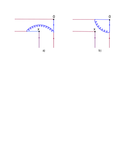
Figure 9: Typical diagrams for one-loop evolution of the quark TMD operator.

$$\langle{\rm T}[0^{+},-\infty]_{x}[-\infty,0^{+}]_{0}\Gamma\psi(0)\rangle_{\Psi}^{\rm Fig.\ref{fig:compare}}~{}=~{}g^{2}c_{F}\!\int\!{\textstyle d}\lower 0.12915pt\hbox{\kern-3.80005pt${}^{\scriptstyle-}$}\kern-0.50003pt{}\beta_{B}{\textstyle d}\lower 0.12915pt\hbox{\kern-3.80005pt${}^{\scriptstyle-}$}\kern-0.50003pt{}p_{B_{\perp}}\Gamma\Psi(\beta_{B})I(\beta_{B},x_{\perp}),$$

$$I(\beta_{B},x_{\perp})~{}=~{}-i\!\int\!{\textstyle d}\lower 0.12915pt\hbox{\kern-3.80005pt${}^{\scriptstyle-}$}\kern-0.50003pt{}\alpha{\textstyle d}\lower 0.12915pt\hbox{\kern-3.80005pt${}^{\scriptstyle-}$}\kern-0.50003pt{}\beta{\textstyle d}\lower 0.12915pt\hbox{\kern-3.80005pt${}^{\scriptstyle-}$}\kern-0.50003pt{}p_{\perp}{1\over\beta+{i\epsilon}}{e^{-i\alpha{\varrho}\delta^{-}}\over\alpha\beta s-p_{\perp}^{2}+{i\epsilon}}{s(\beta-\beta_{B})\over\alpha(\beta-\beta_{B})s-p_{\perp}^{2}+{i\epsilon}}\big{(}1-e^{i(p,x)_{\perp}}\big{)}\Gamma\Psi(\beta_{B})$$ (191)

Without the cutoff in $\alpha$, the integral

$$I(\beta_{B},x_{\perp})~{}=~{}-i\mu^{-2{\varepsilon}}\!\int\!{\textstyle d}\lower 0.12915pt\hbox{\kern-3.80005pt${}^{\scriptstyle-}$}\kern-0.50003pt{}\alpha{\textstyle d}\lower 0.12915pt\hbox{\kern-3.80005pt${}^{\scriptstyle-}$}\kern-0.50003pt{}\beta{\textstyle d}\lower 0.12915pt\hbox{\kern-3.80005pt${}^{\scriptstyle-}$}\kern-0.50003pt{}p_{\perp}{1\over\beta+{i\epsilon}}{1\over\alpha\beta s-p_{\perp}^{2}+{i\epsilon}}{s(\beta_{B}-\beta)\over\alpha(\beta_{B}-\beta)s+p_{\perp}^{2}-{i\epsilon}}\big{(}1-e^{i(p,x)_{\perp}}\big{)}$$

$$=~{}-\mu^{-2{\varepsilon}}\!\int\!{{\textstyle d}\lower 0.12915pt\hbox{\kern-3.80005pt${}^{\scriptstyle-}$}\kern-0.50003pt{}p_{\perp}\over p_{\perp}^{2}}\big{(}1-e^{i(p,x)_{\perp}}\big{)}\!\int_{0}^{\beta_{B}}{\!{\textstyle d}\lower 0.12915pt\hbox{\kern-3.80005pt${}^{\scriptstyle-}$}\kern-0.50003pt{}\beta\over\beta_{B}}{\beta_{B}-\beta\over\beta+{i\epsilon}}~{}=~{}{1\over 8\pi^{2}}{\Gamma({\varepsilon})\over(x_{\perp}^{2}\mu^{2})^{\varepsilon}}\!\int_{0}^{\beta_{B}}\!{d\beta\over\beta_{B}}{\beta_{B}-\beta\over\beta}$$ (192)

diverges as $\beta\rightarrow 0$ even at ${\varepsilon}\neq 0$. The so-called $\delta$-regularization with $A^{-}(z^{+})\rightarrow A^{-}(z^{+})e^{\pm\delta z^{+}}$ gives

$$[0^{+},-\infty]_{x}[-\infty,0^{+}]_{0}~{}\rightarrow~{}i\!\int_{-\infty}^{0}\!dz^{+}[-A^{-}(z^{+},x_{\perp})+A^{-}(z^{+},0_{\perp})]e^{\delta z^{+}}$$ (193)

so that

$$I^{\delta}(\beta_{B},x_{\perp})~{}=~{}{1\over 8\pi^{2}}{\Gamma({\varepsilon})\over(x_{\perp}^{2}\mu^{2})^{\varepsilon}}\!\int_{0}^{\beta_{B}}\!{d\beta\over\beta_{B}}{\beta_{B}-\beta\over\beta+i\delta}~{}\simeq~{}-{1\over 8\pi^{2}}\Big{(}-{1\over{\varepsilon}}+\ln{\mu^{2}x_{\perp}^{2}\over 4}+\gamma\Big{)}\big{(}\ln{\beta_{B}\over i\delta}-1\big{)}$$ (194)

which gives

$$I^{\delta}(\beta_{B},x_{\perp})~{}=~{}{1\over 8\pi^{2}}{\Gamma({\varepsilon})\over(x_{\perp}^{2}\mu^{2})^{\varepsilon}}\!\int_{0}^{\beta_{B}}\!{d\beta\over\beta_{B}}{\beta_{B}-\beta\over\beta-i\delta}~{}\simeq~{}-{1\over 8\pi^{2}}\Big{(}\ln{\mu^{2}x_{\perp}^{2}\over 4}+\gamma\Big{)}\big{(}\ln{\beta_{B}\over i\delta}-1\big{)}$$ (195)

after subtraction of the counterterm.

On the other hand, the rapidity-only cutoff $\delta^{-}={1\over{\varrho}\sigma}$ gives [see Eq. (156)]

$$I^{\sigma}(\beta_{B},x_{\perp})~{}=~{}-i\!\int\!{\textstyle d}\lower 0.12915pt\hbox{\kern-3.80005pt${}^{\scriptstyle-}$}\kern-0.50003pt{}\alpha{\textstyle d}\lower 0.12915pt\hbox{\kern-3.80005pt${}^{\scriptstyle-}$}\kern-0.50003pt{}\beta{\textstyle d}\lower 0.12915pt\hbox{\kern-3.80005pt${}^{\scriptstyle-}$}\kern-0.50003pt{}p_{\perp}{1\over\beta+{i\epsilon}}{e^{-i{\alpha\over\sigma}}\over\alpha\beta s-p_{\perp}^{2}+{i\epsilon}}{s(\beta-\beta_{B})\over\alpha(\beta-\beta_{B})s-p_{\perp}^{2}+{i\epsilon}}\big{(}1-e^{i(p,x)_{\perp}}\big{)}$$

$$=~{}\!\int\!{{\textstyle d}\lower 0.12915pt\hbox{\kern-3.80005pt${}^{\scriptstyle-}$}\kern-0.50003pt{}p_{\perp}\over p_{\perp}^{2}}\big{(}1-e^{i(p,x)_{\perp}}\big{)}\!\int_{0}^{\infty}\!{\textstyle d}\lower 0.12915pt\hbox{\kern-3.80005pt${}^{\scriptstyle-}$}\kern-0.50003pt{}\alpha{\beta_{B}s\over\alpha\beta_{B}s+p_{\perp}^{2}}e^{-i{\alpha\over\sigma}}~{}=~{}-{1\over 16\pi^{2}}\ln^{2}\big{(}-i\beta_{B}\sigma s{x_{\perp}^{2}\over 4}e^{\gamma}\big{)}$$ (196)

The integrals (195) and (196) coincide when $\mu^{2}$ is two times BLM scale $\mu^{2}=2\mu_{\sigma}^{2}=2x_{\perp}^{-1}\sqrt{\beta_{B}\sigma s}$ and $\delta={4\over\sigma sx_{\perp}^{2}}$. Hopefully, the double evolution Echevarria:2015usa along the line $\mu^{2}x^{2}\sqrt{\delta}=4\sqrt{\beta}_{B}$ will produce results compatible with Eq. (132).

VII.7 Rapidity-only evolution beyond Sudakov region at small and moderate $x$

As we demonstrated in this paper, the Sudakov double logs are universal and the evolution of quark and gluon TMDs is the same for low and moderate $x$ until $\sigma\beta_{B}s\sim b_{\perp}^{-2}\sim q_{\perp}^{2}$. From that point, the evolution (or the lack of it) depends on $\beta_{B}=x_{B}$ and $q_{\perp}^{2}$. There are three different scenarios. We will consider them for the case of gluon TMDs since we can use the explicit formulas for the leading-order rapidity evolution at arbitrary $\beta_{B}=x_{B}$ from Ref. Balitsky:2015qba .

First, if $x_{B}\sim 1$ and $q_{\perp}^{2}\gtrsim m_{N}^{2}$, there is no room for any evolution and one should turn to phenomenological models of TMDs such as the replacement of $b$ by $b_{\ast}$ in Refs. Collins:1984kg ; Collins:2017oxh .

If $x_{B}\sim 1$ and $q_{\perp}^{2}\gg m_{N}^{2}$, there is room for DGLAP-type evolution summing logs $\big{(}\alpha_{s}\ln{q_{\perp}^{2}/m_{N}^{2}}\big{)}^{n}$. The rapidity evolution in this case has the form Balitsky:2015qba

$$\sigma{d\over d\sigma}\langle p_{N}|\mathscr{F}^{i,a;\sigma}(\beta_{B},x_{\perp})\mathscr{F}^{a;\sigma}_{~{}~{}i}(\beta_{B},0_{\perp})|p_{N}\rangle$$ (197)

$$\hskip 5.69054pt=~{}4\alpha_{s}N_{c}\!\int\!dk_{\perp}~{}\bigg{\{}e^{i(k,x)_{\perp}}\langle p_{N}|\mathscr{F}^{i,a;\sigma}\big{(}\beta_{B}+{k_{\perp}^{2}\over\sigma s},x_{\perp}\big{)}\mathscr{F}^{a;\sigma}_{~{}~{}i}\big{(}\beta_{B}+{k_{\perp}^{2}\over\sigma s},0_{\perp}\big{)}|p_{N}\rangle\theta\big{(}1-\beta_{B}-{k_{\perp}^{2}\over\sigma s}\big{)}$$

$$\times~{}\Big{[}{1\over k_{\perp}^{2}}-{2\over\sigma\beta_{B}s+k_{\perp}^{2}}+{(\sigma\beta_{B}s)^{2}\over(\sigma\beta_{B}s+k_{\perp}^{2})^{4}}\Big{]}-{\sigma\beta_{B}s\over k_{\perp}^{2}(\sigma\beta_{B}s+k_{\perp}^{2})}\langle p_{N}|\mathscr{F}^{i,a;\sigma}(\beta_{B},x_{\perp})\mathscr{F}^{a;\sigma}_{~{}~{}i}(\beta_{B},y_{\perp})|p_{N}\rangle\bigg{\}}$$

Note that if $\sigma\beta_{B}s\gg x_{\perp}^{-2}$ we get leading-order equation (101) at $\beta=\beta^{\prime}$. On the other hand, as demonstrated in Ref. Balitsky:2015qba , if $\sigma\ll{q_{\perp}^{2}\over\beta_{B}s}$ the factor $e^{i(k,x)_{\perp}}$ in the RHS of Eq. (197) can be neglected and we have the leading-order DGLAP equation with identification $\mu^{2}_{\rm DGLAP}=\sigma\beta_{B}s$. The result of this DGLAP evolution should be convoluted with Eq. (130) using full Eq. (197) for proper matching.

Similarly, if $x_{B}=\beta_{B}\ll 1$, even at $\beta_{B}\sigma s=q_{\perp}^{2}$ there is room for BFKL-type evolution from $\sigma={q_{\perp}^{2}\over\beta_{B}s}$ to $\sigma={q_{\perp}^{2}\over s}$ which corresponds to summing logs $(\alpha_{s}\ln x_{B})^{n}$. The leading-order rapidity equation at arbitrary $\beta_{B}$ has the form Balitsky:2015qba

$$\sigma{d\over d\sigma}\langle p_{N}|\mathscr{F}^{i,a;\sigma}(\beta_{B},x_{\perp})\mathscr{F}^{a;\sigma}_{~{}~{}i}(\beta_{B},0_{\perp})|p_{N}\rangle$$ (198)

$$\hskip 5.69054pt=~{}4\alpha_{s}\!\int\!dk_{\perp}~{}\bigg{[}\theta\big{(}1-\beta_{B}-{k_{\perp}^{2}\over\sigma s}\big{)}\langle p_{N}|N_{c}\mathscr{F}^{i,a;\sigma}\big{(}\beta_{B}+{k_{\perp}^{2}\over\sigma s},x_{\perp}\big{)}\mathscr{F}^{a;\sigma}_{~{}~{}i}\big{(}\beta_{B}+{k_{\perp}^{2}\over\sigma s},0_{\perp}\big{)}|p_{N}\rangle{e^{i(k,x)_{\perp}}\over k_{\perp}^{2}}$$

$$-4N_{c}{\sigma\beta_{B}s\over k_{\perp}^{2}(\sigma\beta_{B}s+k_{\perp}^{2})}\langle p_{N}|\mathscr{F}^{i,a;\sigma}(\beta_{B},x_{\perp})\mathscr{F}^{a;\sigma}_{~{}~{}i}(\beta_{B},y_{\perp})|p_{N}\rangle-\theta\big{(}1-\beta_{B}-{k_{\perp}^{2}\over\sigma s}\big{)}$$

$$\times~{}\langle p_{N}|{\rm Tr}(x_{\perp}|U{p_{j}\over\sigma\beta_{B}s+p_{\perp}^{2}}U^{\dagger}\mathscr{F}^{i,a;\sigma}\big{(}\beta_{B}+{k_{\perp}^{2}\over\sigma s}\big{)}|k_{\perp})(k_{\perp}|\mathscr{F}^{a;\sigma}_{~{}~{}i}\big{(}\beta_{B}+{k_{\perp}^{2}\over\sigma s}\big{)}U{p^{j}\over\sigma\beta_{B}s+p_{\perp}^{2}}U^{\dagger}|y_{\perp})|p_{N}\rangle+~{}\dots$$

where $U(x_{\perp})\equiv[x_{\perp}-\infty^{+},x_{\perp}+\infty^{+}]$ is a Wilson line (infinite gauge link) and dots stand for a number of nonlinear terms similar to the last one [see Eq. (5.5) from Ref. Balitsky:2015qba ]. The small-$x$ evolution is relevant from $\sigma={q_{\perp}^{2}\over\beta_{B}s}$ to $\sigma={q_{\perp}^{2}\over s}$. As demonstrated in Ref. Balitsky:2015qba , at $\sigma\ll{q_{\perp}^{2}\over\beta_{B}s}$ the evolution equation (198) reduces to the BK equation which can be studied using standard small-$x$ methods. After that, the matching of the double-log Sudakov evolution (102) to a single-log BK evolution should be done using full nonlinear equation (198).

References

- (1)
- (2) S. J. Brodsky, G. P. Lepage and P. B. Mackenzie, Phys. Rev. D 28, 228 (1983) doi:10.1103/PhysRevD.28.228
- (3) J. C. Collins and D. E. Soper, Nucl. Phys. B 194, 445-492 (1982) doi:10.1016/0550-3213(82)90021-9
- (4) J. C. Collins, D. E. Soper and G. F. Sterman, Nucl. Phys. B 250, 199-224 (1985) doi:10.1016/0550-3213(85)90479-1
- (5) X. d. Ji, J. p. Ma and F. Yuan, Phys. Rev. D 71, 034005 (2005) doi:10.1103/PhysRevD.71.034005 [arXiv:hep-ph/0404183 [hep-ph]].
- (6) M. G. Echevarria, A. Idilbi and I. Scimemi, JHEP 07, 002 (2012) doi:10.1007/JHEP07(2012)002 [arXiv:1111.4996 [hep-ph]].
- (7) J. Collins, Camb. Monogr. Part. Phys. Nucl. Phys. Cosmol. 32, 1-624 (2011)
- (8) J. C. Collins, Acta Phys. Polon. B 34, 3103 (2003) [arXiv:hep-ph/0304122 [hep-ph]].
- (9) I. Balitsky and A. Tarasov, JHEP 10, 017 (2015) doi:10.1007/JHEP10(2015)017 [arXiv:1505.02151 [hep-ph]].
- (10) I. Balitsky and A. Tarasov, JHEP 06, 164 (2016) doi:10.1007/JHEP06(2016)164 [arXiv:1603.06548 [hep-ph]].
- (11) I. Balitsky and G. A. Chirilli, Phys. Rev. D 100, no.5, 051504 (2019) doi:10.1103/PhysRevD.100.051504 [arXiv:1905.09144 [hep-ph]].
- (12) M. Beneke and V. M. Braun, Phys. Lett. B 348, 513-520 (1995) doi:10.1016/0370-2693(95)00184-M [arXiv:hep-ph/9411229 [hep-ph]].
- (13) S. J. Brodsky, V. S. Fadin, V. T. Kim, L. N. Lipatov and G. B. Pivovarov, JETP Lett. 70, 155-160 (1999) doi:10.1134/1.568145 [arXiv:hep-ph/9901229 [hep-ph]].
- (14) I. Balitsky, Phys. Rev. D 75, 014001 (2007) doi:10.1103/PhysRevD.75.014001 [arXiv:hep-ph/0609105 [hep-ph]].
- (15) Y. V. Kovchegov and H. Weigert, Nucl. Phys. A 784, 188-226 (2007) doi:10.1016/j.nuclphysa.2006.10.075 [arXiv:hep-ph/0609090 [hep-ph]].
- (16) J. Collins and T. Rogers, Phys. Rev. D 91, no.7, 074020 (2015) doi:10.1103/PhysRevD.91.074020 [arXiv:1412.3820 [hep-ph]].
- (17) I. Balitsky and A. Tarasov, JHEP 07, 095 (2017) doi:10.1007/JHEP07(2017)095 [arXiv:1706.01415 [hep-ph]].
- (18) I. Balitsky and A. Tarasov, JHEP 05, 150 (2018) doi:10.1007/JHEP05(2018)150 [arXiv:1712.09389 [hep-ph]].
- (19) I. Balitsky, JHEP 05, 046 (2021) doi:10.1007/JHEP05(2021)046 [arXiv:2012.01588 [hep-ph]].
- (20) I. Balitsky and G. A. Chirilli, Phys. Rev. D 77, 014019 (2008) doi:10.1103/PhysRevD.77.014019 [arXiv:0710.4330 [hep-ph]].
- (21) I. Balitsky and G. A. Chirilli, Nucl. Phys. B 822, 45-87 (2009) doi:10.1016/j.nuclphysb.2009.07.003 [arXiv:0903.5326 [hep-ph]].
- (22) I. I. Balitsky and V. M. Braun, Nucl. Phys. B 311, 541-584 (1989) doi:10.1016/0550-3213(89)90168-5
- (23) P. J. Mulders and J. Rodrigues, Phys. Rev. D 63, 094021 (2001) doi:10.1103/PhysRevD.63.094021 [arXiv:hep-ph/0009343 [hep-ph]].
- (24) A. H. Mueller, B. W. Xiao and F. Yuan, Phys. Rev. Lett. 110, no.8, 082301 (2013) doi:10.1103/PhysRevLett.110.082301 [arXiv:1210.5792 [hep-ph]].
- (25) A. H. Mueller, B. W. Xiao and F. Yuan, Phys. Rev. D 88, no.11, 114010 (2013) doi:10.1103/PhysRevD.88.114010 [arXiv:1308.2993 [hep-ph]].
- (26) D. Gutiérrez-Reyes, I. Scimemi and A. A. Vladimirov, Phys. Lett. B 769, 84-89 (2017) doi:10.1016/j.physletb.2017.03.031 [arXiv:1702.06558 [hep-ph]].
- (27) Y. Li, D. Neill and H. X. Zhu, Nucl. Phys. B 960, 115193 (2020) doi:10.1016/j.nuclphysb.2020.115193 [arXiv:1604.00392 [hep-ph]].
- (28) T. Gehrmann, T. Luebbert and L. L. Yang, JHEP 06, 155 (2014) doi:10.1007/JHEP06(2014)155 [arXiv:1403.6451 [hep-ph]].
- (29) D. Gutierrez-Reyes, I. Scimemi and A. Vladimirov, JHEP 07, 172 (2018) doi:10.1007/JHEP07(2018)172 [arXiv:1805.07243 [hep-ph]].
- (30) M. G. Echevarria, I. Scimemi and A. Vladimirov, Phys. Rev. D 93, no.1, 011502 (2016) [erratum: Phys. Rev. D 94, no.9, 099904 (2016)] doi:10.1103/PhysRevD.93.011502 [arXiv:1509.06392 [hep-ph]].
- (31) J. Collins and T. C. Rogers, Phys. Rev. D 96, no.5, 054011 (2017) doi:10.1103/PhysRevD.96.054011 [arXiv:1705.07167 [hep-ph]].