Search for new cosmic-ray acceleration sites within the 4FGL catalog Galactic plane sources

Abstract

Cosmic rays are mostly composed of protons accelerated to relativistic speeds. When those protons encounter interstellar material, they produce neutral pions which in turn decay into gamma rays. This offers a compelling way to identify the acceleration sites of protons. A characteristic hadronic spectrum, with a low-energy break around 200 MeV, was detected in the gamma-ray spectra of four Supernova Remnants (SNRs), IC 443, W44, W49B and W51C, with the Fermi Large Area Telescope. This detection provided direct evidence that cosmic-ray protons are (re-)accelerated in SNRs. Here, we present a comprehensive search for low-energy spectral breaks among 311 4FGL catalog sources located within 5^∘ from the Galactic plane. Using 8 years of data from the Fermi Large Area Telescope between 50 MeV and 1 GeV, we find and present the spectral characteristics of 56 sources with a spectral break confirmed by a thorough study of systematic uncertainty. Our population of sources includes 13 SNRs for which the proton-proton interaction is enhanced by the dense target material; the high-mass $\gamma$-ray binary LS I +61 303; the colliding wind binary $\eta$ Carinae; and the Cygnus star-forming region. This analysis better constrains the origin of the $\gamma$-ray emission and enlarges our view to potential new cosmic-ray acceleration sites.

1 Introduction

The acceleration site of protons, the main components of cosmic rays, is one of the most fundamental topics of high energy astrophysics. The strong shocks associated with supernova remnants (SNRs) are widely believed to accelerate the bulk of Galactic cosmic rays (E $<10^{15}$ eV) through the diffusive shock acceleration mechanism (e.g. Drury, 1983). Indeed, accelerated cosmic rays interact with surrounding matter and produce $\pi^{0}$ mesons which usually quickly decay into two gamma rays, each having an energy of $67.5$ MeV in the rest frame of the neutral pion. In turn, the gamma-ray number spectrum $F(E)$ is symmetric at this same energy in log-log representation (Stecker, 1971) which then leads to a $\gamma$-ray spectrum in the usual $E^{2}F(E)$ representation rising below 200 MeV and approximately tracing the energy distribution of parent protons at energies greater than a few GeV. This characteristic spectral feature, often referred to as the ”pion-decay bump”, uniquely identifies proton acceleration since leptonic $\gamma$-ray production mechanisms such as bremsstrahlung and inverse Compton (IC) emission require fine tuning to produce a similar feature. Esposito et al. (1996) explored this hypothesis by studying the $\gamma$-ray emission from SNRs, and potential associations of $\gamma$-ray sources with five radio-bright shell-type SNRs were reported using data taken by the EGRET instrument on board the Compton Gamma Ray Observatory. More recently, this signature of protons was detected in five SNRs interacting with molecular clouds (MCs) and detected at gamma-ray energies by Fermi-LAT: IC 443 and W44 (Giuliani et al., 2011; Ackermann et al., 2013), W49B (H. E. S. S. Collaboration et al., 2018a), W51C (Jogler & Funk, 2016) and HB 21 (Ambrogi et al., 2019), although in this last source both the leptonic and hadronic processes are able to reproduce the $\gamma$-ray emission. Finally, the young SNR Cassiopeia A was also analyzed at low energy and Yuan et al. (2013) derived an energy break at $1.72^{+1.35}_{-0.89}$ GeV which is better reproduced by a hadronic scenario. More details on this characteristic feature observed in the gamma-ray emission are provided in Appendix A, showing a stronger signature for a soft proton injection index ($\Gamma=2.5$) than for a hard index ($\Gamma=1.5$).

Electrons can also radiate at gamma-ray energies via the inverse Compton scattering and bremsstrahlung processes. It has been demonstrated, for the supernova remnants interacting with molecular clouds cited above, that the large gamma-ray luminosity is difficult to explain via inverse Compton scattering. In addition, the steep gamma-ray spectrum detected at low energy requires additional breaks in the electron spectrum if we consider a model in which electron bremsstrahlung is dominant. Accurate estimation of the spectral characteristics of a $\gamma$-ray source at low energy is therefore crucial since it probes the nature of the particles (electrons or protons) emitting these gamma rays. However, the analysis of sources below 100 MeV is complicated due to large uncertainties in the arrival directions of the gamma rays, which lead to confusion among point sources and difficulties in separating point sources from diffuse emission. Thus, catalogs released by the Fermi-LAT Collaboration have focused on energies greater than 100 MeV until the 4FGL catalog (Abdollahi et al., 2020) expanded the lower bound to 50 MeV. This allows better constraint of low-energy spectra, but since the 4FGL upper energy bound is 1 TeV, the spectral model for most sources is dominated by data with energies above a few hundred MeV. In addition, the spectral representation of sources in the 4FGL catalog considered three spectral models: power law (PL), power law with sub-exponential cutoff, and log-normal (or log-parabola, hereafter called LP). This means that any source presenting a spectral break will be represented by a log-normal shape which may not adequately represent the low-energy behavior. Similarly, sources presenting two spectral breaks, as it is the case for W49B (H. E. S. S. Collaboration et al., 2018a) will be represented with a log-normal shape that better describes the high-energy interval due to the better angular resolution and increased effective area at these high energies. This directly implies that the description of the low-energy spectral parameters of a source requires a dedicated spectral analysis.

In this paper we use 8 years of Pass 8 data to analyse 311 Galactic sources detected in the 4FGL catalog and search for significant spectral breaks between 50 MeV and 1 GeV. The paper is organized as follows: Section 2 describes the LAT and the observations used, Section 3 presents our systematic methods for analyzing LAT sources in the plane at low energy, Section 4 discusses the main results and a summary is provided in Section 5.

2 Fermi-LAT description and observations

2.1 Fermi-LAT

The Fermi-LAT is a $\gamma$-ray telescope which detects photons with energies from 20 MeV to more than 500 GeV by conversion into electron-positron pairs, as described in Atwood et al. (2009). The LAT is composed of three primary detector subsystems: a high-resolution converter/tracker (for direction measurement of the incident $\gamma$ rays), a CsI(Tl) crystal calorimeter (for energy measurement), and an anti-coincidence detector to identify the background of charged particles. Since the launch of the spacecraft in June 2008, the LAT event-level analysis has been upgraded several times to take advantage of the increasing knowledge of how the Fermi-LAT functions as well as the environment in which it operates. Following the Pass 7 data set, released in August 2011, Pass 8 is the latest version of the Fermi-LAT data. Its development is the result of a long-term effort aimed at a comprehensive revision of the entire event-level analysis and comes closer to realizing the full scientific potential of the LAT (Atwood et al., 2013). The current version of the LAT data is Pass 8 P8R3 (Atwood et al., 2013; Bruel et al., 2018). It offers 20% more acceptance than P7REP (Bregeon et al., 2013). We used the SOURCE class event selection, with the Instrument Response Functions (IRFs) P8R3_SOURCE_V3.

2.2 Data selection and reduction

We used exactly the same dataset as that used to derive the 4FGL catalog of sources, namely 8 years (2008 August 4 to 2016 August 2) of Pass 8 SOURCE class photons. This means that similarly to the 4FGL dataset, our data were filtered removing time periods when the rocking angle was greater than 90^∘ and intervals around solar flares and bright GRBs were excised.
Pass 8 introduced a new partition of the events, called PSF event types, based on the quality of the angular reconstruction, with approximately equal effective area in each event type at all energies. Due to the very low signal to noise ratio at low energy, the angular resolution is critical to distinguish point sources from the background and we decided to use only PSF3 events (the best-quality events) below 100 MeV. We add PSF2 events between 100 MeV and 1 GeV. This high energy bound was selected since middle-aged SNRs commonly exhibit a high energy spectral break at around 1–10 GeV which would then bias our low energy analysis (Uchiyama et al., 2010). For both PSF3 and PSF2 events, we excised photons detected with zenith angles larger than 80^∘ to limit the contamination from $\gamma$ rays generated by cosmic-ray interactions in the upper layers of the atmosphere. That procedure eliminates the need for a specific Earth limb component in the model.
The data reduction and exposure calculations are performed using the LAT $fermitools$ version 1.2.23 and $fermipy$ (Wood et al., 2017) version 0.19.0. We used only binned likelihood analysis because unbinned mode is much more CPU intensive and does not support energy dispersion.
We accounted for the effect of energy dispersion (reconstructed event energy not equal to the true energy of the incoming $\gamma$ ray) which becomes significant at low energies (see below). To do so, we used edisp_bins=-3 which means that the energy dispersion correction operates on the spectra with three extra bins below and above the threshold of the analysis.
Our binned analysis includes three logarithmically spaced energy bins between 50 MeV and 100 MeV, and 9 energy bins between 100 MeV and 1 GeV. The Galactic diffuse emission was modeled by the standard file gll_iem_v07.fits and the residual background and extragalactic radiation were described by an isotropic component (depending on the PSF event type) with the spectral shape in the tabulated model iso_P8R3_SOURCE_V3_PSF(3/2)_v1.txt. The models are available from the Fermi Science Support Center (FSSC). In the following, we fit the normalizations of the Galactic diffuse and the isotropic components.

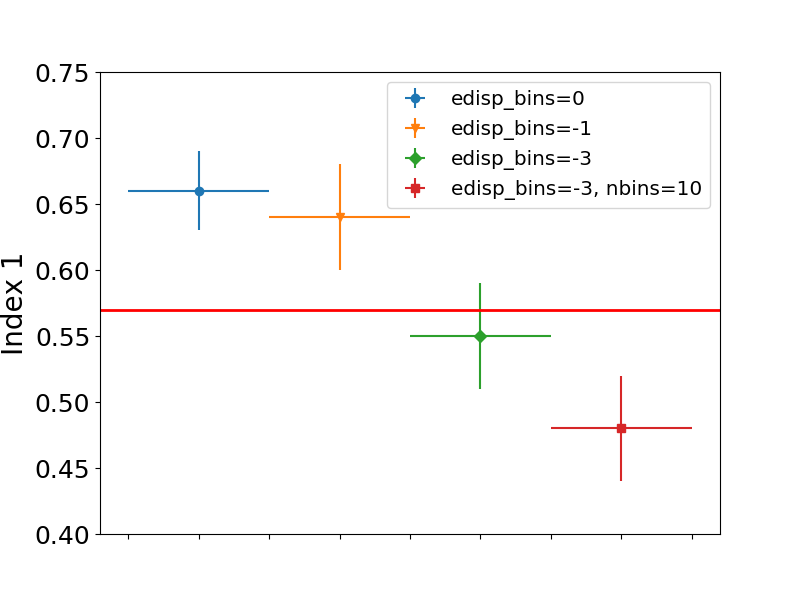
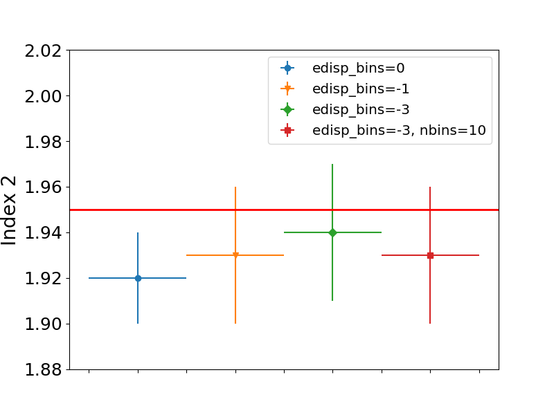
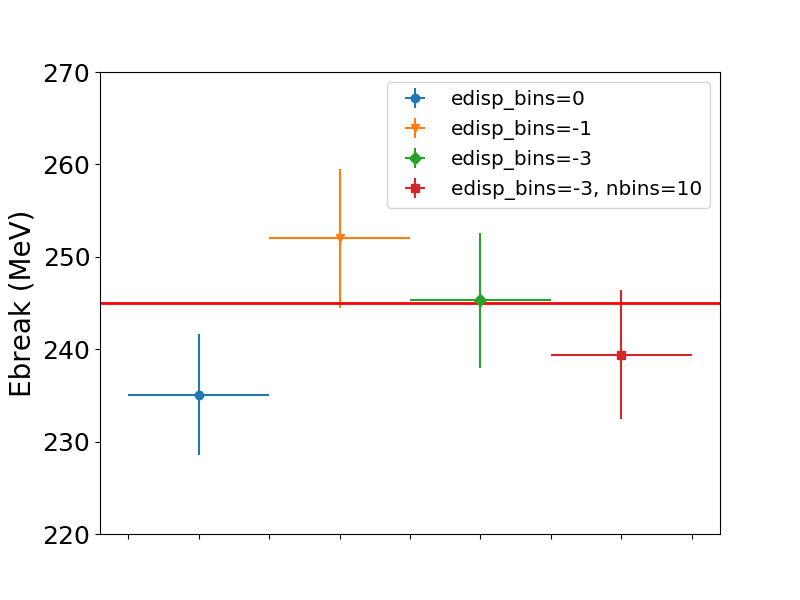
Figure 1: Effect of the number of energy bins and value of edisp_bins on the reconstructed values of the spectral index $\Gamma_{1}$ (left), $\Gamma_{2}$ (middle) and the break energy (right) of the broken power-law model of IC 443. Four configurations are tested: 12 energy bins and edisp_bins = 0 (blue circle), 12 energy bins and edisp_bins = $-1$ (orange triangle), 12 energy bins and edisp_bins = $-3$ (green diamond), 10 energy bins and edisp_bins = $-3$ (red square).

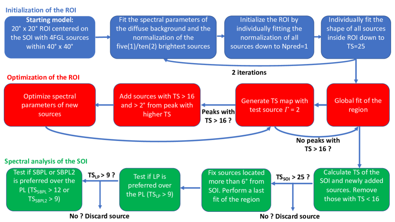
Figure 2: Flow chart illustrating the individual analysis procedure of each source of interest (SOI) located in a $20^{\circ}\times 20^{\circ}$ region of interest. See text for further details.

2.3 Effect of the energy dispersion

A crucial point that needs to be considered when analyzing LAT data at low energies is the effect of energy dispersion. For Pass 8, the energy resolution is $<10$% between 1 GeV and 100 GeV but it worsens below 1 GeV. It is $\sim 20$% at 100 MeV and $\sim 28$% at 30 MeV. The combination of energy dispersion and the rapidly changing effective area below 100 MeV could result in biased measurements of flux and spectral index of the source under study. In order to quantify the effects of energy dispersion, 200 simulations of the spectrum of IC 443 as published by Ackermann et al. (2013) were performed for a 8-year observation time using the $gtobssim$ tool included in the LAT $fermitools$. For these simulations, we assumed a point source spatial model located at (RA, Dec (J2000): 94.51^∘, 22.66^∘) and a smooth broken power-law spectral model of the form:

$$\frac{dN}{dE}=N_{0}(E/E_{0})^{-\Gamma_{1}}(1+(E/E_{\rm br})^{(\Gamma_{2}-\Gamma_{1})/\alpha})^{-\alpha},$$ (1)

where $\alpha=0.1$, the break energy $E_{\rm br}=245$ MeV and the spectral indices $\Gamma_{1}=0.57$, $\Gamma_{2}=1.95$. These simulations include the effect of energy dispersion. The analysis of these simulations was performed with the exact same configuration (region size, PSF components used, spatial bin size, energy interval) as the one used for real data. The only two parameters that have been varied in this study are the number of energy intervals and the value of the parameter edisp_bins as discussed in Section 2.2. For each combination of (energy bins, edisp_bins), we analyzed the 200 simulations, plotted the distributions of the reconstructed values of the break energy, $\Gamma_{1}$ and $\Gamma_{2}$ and fitted a Gaussian on each distribution.
The centroid of the Gaussian fit together with their size are reported in Figure 1 for the four tests performed: (12 energy bins, edisp_bins = 0), (12 energy bins, edisp_bins = $-1$), (12 energy bins, edisp_bins = $-3$), (10 energy bins, edisp_bins = $-3$). As can be seen on this Figure, the main effect is on $\Gamma_{1}$, as expected. If the energy dispersion is not taken into account (edisp_bins = 0), the spectrum is less steeply falling at low energy and the spectral index $\Gamma_{1}$ is reconstructed with a value 0.1 higher than the simulated value set in the simulations. This is also true if the energy dispersion is taken into account with only one extra bin (edisp_bins = -1) which is not sufficient to properly take into account the effect of energy dispersion at these low energies even if this configuration has the advantage to reproduce slightly more accurately the value of the break energy. Even with a configuration using edisp_bins=-3, if the number of bins is too small, the reconstructed value of $\Gamma_{1}$ will be biased towards lower value which will create artificially a stronger break at low energy. This is directly due to the fact that the energy resolution varies with energy. This imposes to choose an energy binning that is fine enough to capture this energy dependence.
The best compromise that was found between good reconstruction and computation time (since higher values of edisp_bins or of the number of energy bins increase the CPU time) was obtained for a configuration using edisp_bins=-3 and 12 energy bins between 50 MeV and 1 GeV. This configuration was used for all results presented in the following.

3 Detection of spectral breaks

3.1 List of candidates

This analysis intends to find new cosmic-ray acceleration sites in our Galaxy. When cosmic-ray protons accelerated by a source penetrate into high density clouds, the gamma-ray emission is expected to be enhanced relative to the interstellar medium because of the more frequent proton-proton interactions. Targeting the presence of such clouds, we restricted our search to sources within $5^{\circ}$ from the Galactic plane. In addition, we removed from our list all identified pulsars and active galactic nuclei. For AGNs, we removed all subclasses, namely flat-spectrum radio quasars (FSRQs), BL Lac-type objects (BLLs), blazar candidates of uncertain type (BCUs), radio galaxies (RDGs), narrow-line Seyfert 1 (NLSY1s), steep spectrum radio quasars (SSRQs), Seyfert galaxies (SEYs) or simply AGNs. Finally, to ensure that the source is significant in the low energy domain covered by our analysis, we removed all sources with a significance below $3\sigma$ between 300 MeV and 1 GeV as reported in the 4FGL catalog. In the end, these selection criteria provide us with a list of 311 candidates reported in the Appendix B.

3.2 Input source model construction

We perform an independent analysis of the 311 candidates selected in Section 3.1. The procedure followed is inspired by the Fermi High-Latitude Extended Sources Catalog (Ackermann et al., 2018), which already used the functions provided by $fermipy$.
For each source of interest, we define a $20^{\circ}\times 20^{\circ}$ region and include in our baseline model all 4FGL sources located in a $40^{\circ}\times 40^{\circ}$ region centered on our source of interest. We model each 4FGL source using the same spectral parameterization as used in the 4FGL. For extended sources, we use the spatial models from the 4FGL and keep them as fixed parameters since the angular resolution between 50 MeV and 1 GeV does not allow us to perform a morphological analysis. Similarly the positions of all point sources are fixed at their 4FGL values.
Starting from the baseline model, we proceed to optimize the model using the optimize function provided by $fermipy$. In this optimization step, we first fit the spectral parameters of the Galactic interstellar emission model and residual background together with the normalization of the five brightest sources.
Then, we individually fit the normalizations of all sources inside the region of interest (ROI) that were not included in the first step in the order of their total predicted counts in the model (Npred) down to Npred = 1. The optimization is concluded by individually fitting the index and normalization parameters of all sources with a test statistic (${\rm TS}$) value above 25 starting from the highest TS sources. This ${\rm TS}$ value is determined from the first two steps of the ROI optimization by ${\rm TS}=2(\ln\mathcal{L}_{1}-\ln\mathcal{L}_{0})$, where $\mathcal{L}_{0}$ and $\mathcal{L}_{1}$ are the likelihoods of the background (null hypothesis) and the hypothesis being tested (source plus background). This optimization is followed by a second one where the number of bright sources fit together with the diffuse backgrounds is increased to 10. This allows a better convergence for complex regions containing a large number of bright sources.
After optimizing the parameters of the baseline model components, we then perform a fit of the region by leaving free the normalization of all sources within $2^{\circ}$ of the source of interest, their spectral shape if their ${\rm TS}$ value is above 16, the normalization of all sources with ${\rm TS}>100$ in the ROI and the spectral shape of all sources in the ROI with ${\rm TS}>200$. If the number of degrees of freedom (Ndof) is above 100, we increase the two last ${\rm TS}$ criteria by 100 until Ndof becomes smaller than 100.
Once this complete fit of the ROI is performed, we further refine the model by identifying and adding new point source candidates. We identify candidates by generating a TS map for a point source that has a PL spectrum with an index $\Gamma=2$. When generating the TS map, we fix the parameters of the background sources and fit only the amplitude of the test source. We add a source at every peak in the TS map with ${\rm TS}>16$ that is at least $2^{\circ}$ from a peak with higher TS due to the poor angular resolution at these low energies. New source candidates are modeled with a PL whose normalization and index are fit in this procedure. We then generate a new TS map after adding the point sources to the model and repeat the procedure until no candidates with ${\rm TS}>16$ are found. Though we do not expect to find a large number of additional sources, this step is crucial since we are not using the weights, first introduced for the 4FGL Catalog (Abdollahi et al., 2020). Indeed, the generation of the candidate list for the Catalog is done above 100 MeV (instead of 50 MeV for our analysis) and each candidate is kept if the TS value obtained via a weighted maximum likelihood fit is above 25. These weights mitigate the effect of systematic errors due to our imperfect knowledge of the Galactic diffuse emission. As a consequence, the TS value of soft sources decreases.
In the final pass of the analysis, a second general fit of the ROI is performed using the same criteria as above to free the spectral parameters of all sources. If sources added previously by using the TS map fall down below ${\rm TS}>16$, they are removed from the model. If their ${\rm TS}$ value is above 16 and they are located at a distance smaller than $5^{\circ}$ from our source of interest, we test iteratively for each of them the improvement of the log-normal representation with respect to the power-law model. The log parabola model is defined as:

$$\frac{dN}{dE}=N_{0}\left(\frac{E}{E_{0}}\right)^{-\left(\alpha+\beta\log\left(E/E_{0}\right)\right)},$$ (2)

where $N_{0}$ is the overall normalisation factor to scale the observed brightness of a source, $E_{0}$ is a fixed scale energy (kept at 300 MeV in our analysis), and $\alpha$, $\beta$ are left free, which adds one degree of freedom with respect to the power-law representation. The improvement of the log-parabola model (LP) with respect to the power law one (PL) is performed by determining ${\rm TS_{LP}}=2(\ln\mathcal{L}_{\rm LP}-\ln\mathcal{L}_{\rm PL})$. If ${\rm TS_{LP}}$ is above 9 (which corresponds to a $3\sigma$ improvement for one additional degree of freedom), we switch to the log-normal representation. The spectral parameters of all added sources located within $5^{\circ}$ of a candidate are reported in Table 1. As can be seen, the curvature index $\beta$ is hard to constrain for the additional faint sources, even if the log-parabola model significantly improves the fit. It is also clear that several added sources are located within the Vela and Cygnus regions for which the morphological templates used for the Vela-X PWN or the Cygnus Cocoon are not precise enough to characterize properly the region. Because the 4FGL Catalog rejects most point sources found inside extended sources, this leaves many residuals which translate into sources.

Table 1: Localization and TS value of added sources localized within 5^∘ of a confirmed candidate with a significant spectral break (the reference energy $E_{0}$ is fixed at 300 MeV in all cases)

Name	RA, Dec	TS value	${\rm TS_{LP}}$	Prefactor	Index	$\beta$
	(∘), (∘)			($10^{-11}$ cm-2s-1MeV-1)
PS J0216.4+6213	34.12, 62.23	31	1	2.1 $\pm$ 0.6	1.8 $\pm$ 0.3
PS J0327.6+5329	51.92, 53.49	30	5	1.0 $\pm$ 0.3	1.7 $\pm$ 0.3
PS J0533.7+2501	83.45, 25.03	72	3	0.8 $\pm$ 0.2	4.2 $\pm$ 0.2
PS J0845.8$-$4448	131.46, $-$44.81	30	4	3.0 $\pm$ 0.7	2.3 $\pm$ 0.2
PS J0838.1$-$4212	129.55, $-$42.21	66	16	5.2 $\pm$ 0.9	2.0 $\pm$ 0.3	1.0
PS J0856.8$-$4245	134.21, $-$42.76	59	5	2.6 $\pm$ 0.2	1.9 $\pm$ 0.1
PS J0900.7$-$4438	135.20, $-$44.64	92	5	2.8 $\pm$ 0.2	1.5 $\pm$ 0.1
PS J1558.2$-$5029	239.56, $-$50.50	51	28	5.5 $\pm$ 0.7	2.7 $\pm$ 0.2	1.0
PS J1603.6$-$4621	240.92, $-$46.35	35	10	2.5 $\pm$ 0.4	2.0 $\pm$ 0.2	1.0
PS J1632.5$-$4221	248.14, $-$42.35	39	7	1.7 $\pm$ 0.3	1.9 $\pm$ 0.1
PS J1642.0$-$4802	250.50, $-$48.05	32	2	3.6 $\pm$ 0.9	2.2 $\pm$ 0.2
PS J1816.9$-$1619	274.23, $-$16.32	46	8	4.9 $\pm$ 0.9	1.8 $\pm$ 0.2
PS J2026.4+4004	306.62, 40.07	88	0	5.7 $\pm$ 0.1	1.8 $\pm$ 0.2
PS J2032.0+3935	308.02, 39.59	131	7	6.6 $\pm$ 0.7	1.9 $\pm$ 0.1
PS J2038.7+4114	309.70, 41.24	87	10	7.4 $\pm$ 0.7	1.8 $\pm$ 0.2	0.7 $\pm$ 0.2
PS J2035.7+4242	308.94, 42.71	50	0	3.5 $\pm$ 0.4	1.7 $\pm$ 0.1
PS J2018.8+4112	304.70, 41.20	74	12	8.9 $\pm$ 1.0	3.0 $\pm$ 0.2	0.5 $\pm$ 0.1
PS J2045.5+4205	311.38, 42.10	48	9	4.9 $\pm$ 0.8	2.0 $\pm$ 0.3	1.0
PS J2045.9+5044	311.48, 50.74	32	4	2.5 $\pm$ 0.5	1.8 $\pm$ 0.2
PS J2047.9+4456	311.99, 44.94	47	6	2.4 $\pm$ 0.4	1.8 $\pm$ 0.2

Note. — Columns 2 and 3 provide the Right Ascension, Declination of the added source and its ${\rm TS}$ value. Column 4 gives the improvement of the lognormal representation with respect to the power-law model ${\rm TS_{LP}}$ as defined in Section 3.2. If ${\rm TS_{LP}}>9$, a lognormal representation is favoured and the Index provided in Column 5 corresponds to the spectral parameter $\alpha$ in Equation 2, while $\beta$ is indicated in Column 6 in such cases. No errors on $\beta$ are reported when it hits the boundary of 1.0.

3.3 Spectral energy breaks

Once the ROI is well characterized, we first test the ${\rm TS}$ value of our source of interest in our energy range (50 MeV to 1 GeV). If it is below 25, we stop the analysis for this source since it is not significantly detected in our pipeline. It is the case for 64 sources among the 311 selected and their ${\rm TS}$ value is reported in Table 8. If the ${\rm TS}$ of the source of interest is above 25, we move on and we fix all sources located more than $5^{\circ}$ from the source of interest and we test the spectral curvature of our source of interest.
To ensure that the curvature is real and affects several energy bins as it would be the case for a “pion-decay bump” signature, we first test a log-normal representation for the source as defined in Equation 2. If ${\rm TS_{LP}}$ is below 9, we consider that no significant curvature is detected by our pipeline, we report this value in Table 8 and we stop the analysis of this source. It is the case for 167 sources in our sample.
If the value is above 9, we then test a smoothly broken power law following Equation 1 where $N_{0}$ is the differential flux at $E_{0}=300$ MeV and $\alpha=0.1$, as was done previously for the cases of IC 443 and W44 (Ackermann et al., 2013). This adds two additional degrees of freedom with respect to the power-law model (the break energy $E_{\rm br}$ and a second spectral index $\Gamma_{2}$). The improvement with respect to the power law one is determined by ${\rm TS_{SBPL}}=2(\ln\mathcal{L}_{\rm SBPL}-\ln\mathcal{L}_{\rm PL})$. Since this test requires the addition of two degrees of freedom to the fit and diffusive shock acceleration predicts $\Gamma_{2}\sim 2$, we also test the improvement of the smooth broken power law with the second index fixed at 2 with respect to the power law one ${\rm TS_{SBPL2}}=2(\ln\mathcal{L}_{\rm SBPL2}-\ln\mathcal{L}_{\rm PL})$. We require ${\rm TS_{SBPL}}>12$ or ${\rm TS_{SBPL2}}>9$ (implying a $3\sigma$ improvement for 2 and 1 additional degrees of freedom respectively) to keep the source in the significant energy break list reported in Table 2. We switch to the SBPL parameterization for all sources detected in this list. This means that, when a source located within $5^{\circ}$ shows a significant energy break, we re-optimize the ROI and we re-do the whole process as illustrated in the flow chart in Figure 2. This procedure allowed the detection of 77 sources presenting a significant energy break in their low-energy spectrum. The values of ${\rm TS_{LP}}$, ${\rm TS_{SBPL}}$, ${\rm TS_{SBPL2}}$ for each of them is reported in Table 8.

3.4 Diffuse and IRF Systematics

The primary source of systematic error in this low energy analysis is the Galactic interstellar emission model (IEM). Our nominal Galactic IEM is the recommended one for PASS 8 source analysis. It represents the first major update to the LAT Collaboration’s IEM since the model for the 3FGL catalog analysis gll_iem_v05.fits, developed for Pass 7 Source class, and later rescaled for Pass 8 Source as gll_iem_v06.fits. The development of the new model is described in more detail (including illustrations of the templates and residuals) online. The new model has higher resolution and correspondingly greater contrast but some shortcomings in the new Galactic IEM have been recognized when producing the 4FGL catalog.
To quantify the impact of diffuse systematics, we repeated our analysis for the 77 sources listed in Table 2 using the old diffuse rescaled for Pass 8 Source gll_iem_v06.fits. This alternative analysis means that the whole flow chart in Figure 2 was performed again, from the optimization of the ROI to the source finding algorithm, up to the determination of the spectral curvature. Performing the same complete analysis with the eight alternate diffuse models from Acero et al. (2016) would have become extremely CPU time consuming and this is why the old diffuse model only is tested. Here, since we already know that the source presents a break with the new model, we directly tested if ${\rm TS_{SBPL}}>12$ or ${\rm TS_{SBPL2}}>9$. If it was not the case, then this source was discarded from the final list of sources presenting significant energy break.

Table 2: Results of the systematic studies

4FGL Name	$\rm TS_{SBPL}$	$\rm TS_{SBPL2}$	$\rm TS_{SBPL}$	$\rm TS_{SBPL2}$	$\rm TS_{SBPL}$	$\rm TS_{SBPL2}$
	diffuse	diffuse	Aeff min	Aeff min	Aeff max	Aeff max
$\star$4FGL J0222.4+6156e	24.3	16.5	34.9	27.5	35.1	27.7
$\star$4FGL J0240.5+6113	170.7	143.5	127.5	123.9	124.0	123.2
$\star$4FGL J0330.7+5845	13.8	7.7	15.8	12.5	16.0	12.5
$\star$4FGL J0340.4+5302	81.6	67.5	147.0	143.5	140.1	138.5
$\star$4FGL J0426.5+5434	13.0	6.9	26.3	21.0	25.6	20.4
$\star$4FGL J0500.3+4639e	12.2	8.1	15.2	14.5	14.9	14.2
$\star$4FGL J0540.3+2756e	12.7	8.0	10.8	10.6	10.7	10.6
$\star$4FGL J0609.0+2006	14.7	6.6	17.6	14.0	17.1	14.1
$\star$4FGL J0617.2+2234e	103.7	81.1	96.5	79.3	95.2	79.5
4FGL J0618.7+1211	10.4	5.7	16.5	9.3	15.2	9.5
$\star$4FGL J0620.4+1445	13.5	6.0	14.0	9.2	14.2	9.3
$\star$4FGL J0634.2+0436e	26.3	21.3	17.6	17.6	10.5	10.6
$\star$4FGL J0639.4+0655e	33.3	28.9	44.8	39.3	45.0	39.4
$\star$4FGL J0709.1$-$1034	26.5	14.6	19.5	13.0	19.4	13.0
4FGL J0722.7$-$2309	11.1	5.5	21.5	10.6	21.6	10.7
4FGL J0731.5$-$1910	9.4	5.1	16.4	9.4	16.3	9.4
$\star$4FGL J0844.1$-$4330	27.1	13.2	38.9	13.2	32.7	11.2
$\star$4FGL J0850.8$-$4239	15.2	9.0	27.4	19.7	27.7	19.9
$\star$4FGL J0904.7$-$4908c	15.8	9.4	11.8	9.7	12.5	10.0
4FGL J0911.6$-$4738	11.8	7.1	11.8	9.7	10.8	8.2
4FGL J0924.1$-$5202	11.9	6.6	16.8	9.2	18.5	9.3
$\star$4FGL J1008.1$-$5706c	21.5	9.9	25.7	20.6	25.7	20.8
$\star$4FGL J1018.9$-$5856	14.7	5.2	28.9	27.9	28.5	28.2
$\star$4FGL J1045.1$-$5940	25.6	19.8	15.2	15.0	17.0	16.9
4FGL J1244.3$-$6233	11.4	8.0	30.9	10.8	31.2	11.1
$\star$4FGL J1351.6$-$6142	13.6	5.7	15.7	14.1	17.9	16.2
$\star$4FGL J1358.3$-$6026	21.7	6.1	22.1	12.8	22.5	13.1
$\star$4FGL J1405.1$-$6119	23.6	16.2	25.1	20.1	25.1	20.1
4FGL J1408.9$-$5845	10.3	5.4	11.5	9.0	11.9	9.1
$\star$4FGL J1442.2$-$6005	15.1	6.5	16.3	12.0	16.6	12.2
$\star$4FGL J1447.4$-$5757	15.4	7.7	18.1	14.4	18.3	14.6
4FGL J1501.0$-$6310e	7.9	3.2	17.8	10.0	18.4	10.1
$\star$4FGL J1514.2$-$5909e	14.0	11.3	34.1	27.8	32.9	29.1
$\star$4FGL J1534.0$-$5232	12.2	5.3	13.6	8.5	13.9	8.4
$\star$4FGL J1547.5$-$5130	17.0	12.9	32.8	16.3	30.8	18.3
$\star$4FGL J1552.9$-$5607e	12.0	7.9	11.5	10.9	11.9	10.9
4FGL J1553.8$-$5325e	7.9	4.1	73.5	63.2	74.0	64.6
4FGL J1556.0$-$4713	9.8	5.8	11.4	4.8	10.2	4.6
$\star$4FGL J1601.3$-$5224	34.2	21.9	42.9	36.9	44.6	36.5
$\star$4FGL J1608.8$-$4803	20.4	13.7	30.8	13.2	30.7	13.4
$\star$4FGL J1626.6$-$4251	20.8	13.9	18.2	8.7	15.2	8.8
$\star$4FGL J1633.0$-$4746e	12.8	8.5	37.2	36.4	38.1	37.1
4FGL J1639.3$-$5146	7.2	4.0	17.2	6.4	18.1	7.1
4FGL J1645.8$-$4533	8.9	6.6	28.9	10.5	30.9	14.6
4FGL J1708.6$-$4312	10.4	6.8	19.6	9.2	19.9	9.4
4FGL J1730.1$-$3422	9.8	1.5	35.6	13.8	35.9	14.1
4FGL J1734.5$-$2818	8.7	4.0	29.9	14.7	35.9	14.1
$\star$4FGL J1742.8$-$2246	18.3	6.8	15.2	8.4	19.5	10.1
4FGL J1743.4$-$2406	7.0	3.8	14.7	5.3	14.9	6.5
4FGL J1759.7$-$2141	10.2	6.0	17.7	6.9	18.0	7.1
$\star$4FGL J1801.3$-$2326e	89.1	83.5	173.9	146.6	175.5	147.6
$\star$4FGL J1808.2$-$1055	13.3	7.9	14.6	10.0	14.6	10.1
$\star$4FGL J1812.2$-$0856	13.8	7.4	15.8	7.8	16.0	13.6
$\star$4FGL J1813.1$-$1737e	17.7	12.9	25.0	18.4	27.5	14.9
$\star$4FGL J1814.2$-$1012	17.7	7.8	20.2	11.1	17.4	11.0
$\star$4FGL J1839.4$-$0553	14.0	9.7	22.2	20.4	22.6	20.9
$\star$4FGL J1852.4+0037e	14.1	4.5	20.3	19.4	22.1	19.9
$\star$4FGL J1855.2+0456	20.8	9.7	31.7	12.2	31.9	12.0
$\star$4FGL J1855.9+0121e	90.0	82.3	91.1	91.5	94.3	94.8
4FGL J1856.2+0749	8.5	4.5	21.1	19.5	19.3	14.8
$\star$4FGL J1857.7+0246e	12.0	5.6	24.4	20.5	24.9	19.1
$\star$4FGL J1906.9+0712	11.3	10.9	28.1	18.7	28.0	19.8
$\star$4FGL J1908.7+0812	15.8	10.3	62.3	41.8	62.9	42.1
$\star$4FGL J1911.0+0905	14.4	10.4	27.8	27.6	27.8	27.4
4FGL J1912.5+1320	7.9	4.0	21.2	14.0	21.8	14.1
$\star$4FGL J1923.2+1408e	23.0	17.7	20.8	20.7	22.3	22.1
$\star$4FGL J1931.1+1656	13.5	7.0	23.1	17.0	23.3	17.3
$\star$4FGL J1934.3+1859	28.4	12.5	31.1	15.6	30.5	14.5
4FGL J1952.8+2924	8.0	4.0	20.6	12.4	21.0	12.6
4FGL J2002.3+3246	8.3	4.1	14.3	11.2	14.3	10.4
$\star$4FGL J2021.0+4031e	31.6	14.6	25.6	10.2	25.8	10.2
$\star$4FGL J2028.6+4110e	49.2	34.3	94.5	91.8	132.9	129.9
$\star$4FGL J2032.6+4053	13.6	15.2	21.3	19.0	22.2	19.2
$\star$4FGL J2038.4+4212	17.0	9.4	14.4	10.3	14.5	10.3
$\star$4FGL J2045.2+5026e	24.6	15.4	37.4	25.7	37.3	26.0
$\star$4FGL J2056.4+4351c	17.2	11.0	18.9	10.0	18.1	10.2
$\star$4FGL J2108.0+5155	13.5	7.1	18.2	12.3	18.3	12.4

Note. — Columns 2 and 3 are obtained with the galactic diffuse background rescaled for Pass 8 Source (gll_iem_v06.fits) and provide values of the improvement of the smooth broken power-law representation with respect to the power-law model ${\rm TS_{SBPL}}$ and the improvement of the smooth broken power-law representation when fixing $\Gamma_{2}=2$ called ${\rm TS_{SBPL2}}$ as defined in Section 3.2. Columns 4, 5, 6 and 7 provide the same values of ${\rm TS_{SBPL}}$ and ${\rm TS_{SBPL2}}$ for the two bracketing IRFs. Stars $\star$ denote spectral breaks that are robust to all tests. See Section 3.4 for more details.

The second source of systematic error in our analysis is the instrument response functions (IRFs) and especially the inaccuracies in the effective area. Following the standard method (Ackermann et al. 2012a), we estimated the systematic error associated with the effective area by calculating uncertainties in the IRFs which symmetrically bracket the standard effective area and flip from one extrema to the other at the measured value of the break energy. Here we started from the best fit model obtained with the standard IRF which is optimized before running the final spectral fit of each candidate with each of the two bracketing IRFs. The source finding algorithm was not relaunched in this case since these changes mainly affect the spectral parameters of the source and will not produce extra sources in the field of view.
A third source of systematic error that can affect the presence or absence of a spectral break for the source of interest is related to the inaccuracy of the emission models of nearby point sources. A thorough investigation of this effect is beyond the scope of this paper but we included in Table 3, for each candidate, the distance of the nearest source as well as the relative contribution of photons from the neighboring sources and from the diffuse backgrounds. Those values show that the diffuse background impacts the sources much more than their neighbors, with the exception of 4FGL J2021.0+4031e around the bright PSR J2021+4026.

Table 3: Fractions of photons from neighboring sources and diffuse background affecting all confirmed sources showing a significant break

4FGL Name	Distance (∘)	$\rm N_{soi}/N_{diff}$	$\rm N_{soi}/N_{srcs}$
4FGL J0222.4+6156e	0.76	0.85	3.61
4FGL J0240.5+6113	1.28	7.34	112.58
4FGL J0330.7+5845	2.51	0.14	22.24
4FGL J0340.4+5302	1.39	0.86	38.35
4FGL J0426.5+5434	0.99	0.68	311.20
4FGL J0500.3+4639e	1.31	0.17	7.70
4FGL J0540.3+2756e	1.35	0.08	1.99
4FGL J0609.0+2006	0.48	0.20	1.78
4FGL J0617.2+2234e	0.40	5.40	28.79
4FGL J0620.4+1445	1.03	0.16	1.56
4FGL J0634.2+0436e	1.29	0.22	2.74
4FGL J0639.4+0655e	1.47	0.09	0.85
4FGL J0709.1$-$1034	1.42	0.25	10.44
4FGL J0844.1$-$4330	0.85	0.25	0.22
4FGL J0850.8$-$4239	0.68	0.29	0.80
4FGL J0904.7$-$4908c	0.66	0.18	1.60
4FGL J1008.1$-$5706c	0.59	0.19	2.76
4FGL J1018.9$-$5856	0.33	2.28	3.39
4FGL J1045.1$-$5940	0.52	1.39	2.76
4FGL J1351.6$-$6142	0.72	0.25	1.78
4FGL J1358.3$-$6026	0.48	0.27	1.32
4FGL J1405.1$-$6119	0.48	0.51	1.51
4FGL J1442.2$-$6005	0.24	0.17	0.95
4FGL J1447.4$-$5757	1.28	0.28	2.97
4FGL J1514.2$-$5909e	0.69	0.24	1.06
4FGL J1534.0$-$5232	1.23	0.12	2.98
4FGL J1547.5$-$5130	0.66	0.17	2.28
4FGL J1552.9$-$5607e	2.25	0.15	6.69
4FGL J1601.3$-$5224	1.46	0.14	3.64
4FGL J1608.8$-$4803	1.30	0.15	1.92
4FGL J1626.6$-$4251	0.75	0.12	1.33
4FGL J1633.0$-$4746e	0.28	0.32	2.44
4FGL J1742.8$-$2246	1.00	0.20	1.22
4FGL J1801.3$-$2326e	0.08	0.70	2.83
4FGL J1808.2$-$1055	1.14	0.17	1.38
4FGL J1812.2$-$0856	1.36	0.21	3.33
4FGL J1813.1$-$1737e	0.50	0.20	2.43
4FGL J1814.2$-$1012	1.29	0.16	1.20
4FGL J1839.4$-$0553	0.28	0.45	0.87
4FGL J1852.4+0037e	0.76	0.15	0.87
4FGL J1855.2+0456	1.25	0.16	2.01
4FGL J1855.9+0121e	0.44	1.25	5.17
4FGL J1857.7+0246e	0.45	0.22	1.34
4FGL J1906.9+0712	0.23	0.26	0.65
4FGL J1908.7+0812	0.94	0.20	1.54
4FGL J1911.0+0905	0.21	0.49	2.81
4FGL J1923.2+1408e	0.35	0.91	3.27
4FGL J1931.1+1656	0.74	0.22	1.92
4FGL J1934.3+1859	0.55	0.21	0.72
4FGL J2021.0+4031e	0.12	0.79	0.19
4FGL J2028.6+4110e	0.73	0.16	0.43
4FGL J2032.6+4053	0.57	0.22	0.46
4FGL J2038.4+4212	0.71	0.24	1.09
4FGL J2045.2+5026e	0.32	0.32	1.77
4FGL J2056.4+4351c	1.07	0.18	3.63
4FGL J2108.0+5155	1.14	0.19	15.44

Note. — Column 1 indicates the distance (in degrees) of the nearest neighboring source. Columns 2 and 3 report the ratio, in the pixel at the source position, between the predicted number of photons from the source of interest with respect to those of the galactic and isotropic diffuse background ($\rm N_{soi}/N_{diff}$), and to those of all neighboring sources $\rm N_{soi}/N_{srcs}$, respectively.

Overall, 56 sources among the 77 sources detected with the standard IEM and IRFs are confirmed with our systematic studies. The 21 candidates rejected are all sources that do not meet the ${\rm TS_{SBPL}}$ or ${\rm TS_{SBPL2}}$ criteria when using the old diffuse model, while the inaccuracy in the effective area has a minor effect in our analysis as can be seen in Table 2. The spectral parameters of the confirmed sources are reported in Table 4. As can be seen in this Table, even if the old diffuse background detects a significant energy break, the energy of this break can be significantly different than with the standard IEM, leading to large systematics as well on $\Gamma_{1}$. However, the value of $\Gamma_{2}$ is much more robust.
In addition to performing a spectral fit over the entire energy range, we computed an SED by fitting the flux of the source independently in 10 energy bins spaced uniformly in log space from 50 MeV to 1 GeV. During this fit, we fixed the spectral index of the source at 2 as well as the model of background sources to the best fit obtained in the whole energy range except the normalizations of the Galactic diffuse and isotropic backgrounds. We determined the flux in an energy bin when TS $\geq 1$ and otherwise computed a 95% confidence level Bayesian flux upper limit, assuming a uniform prior on flux following Helene (1983). The systematic studies with the old diffuse and bracketing IRFs were also computed on all SED points for the 56 confirmed sources and the two uncertainties were added in quadrature. When an upper limit was derived, the maximal and minimal upper limits derived in this energy interval are plotted to indicate the systematics related to this data point.

Table 4: Spectral parameters of all confirmed sources showing a significant break

4FGL Name	$\rm I(50-1000)$	$\rm\Delta I(50-1000)$	$\rm E_{break}$	$\rm\Delta E_{break}$	$\rm\Gamma_{1}$	$\rm\Delta\Gamma_{1}$	$\rm\Gamma_{2}$	$\rm\Delta\Gamma_{2}$
	$10^{-6}$ (MeV/cm2/s)	stat/syst	(MeV)	stat/syst		stat/syst		stat/syst
4FGL J0222.4+6156e	47.8	2.7/0.6	465	78/40	1.35	0.14/0.03	2.34	0.21/0.14
4FGL J0240.5+6113	237.6	1.9/6.6	142	10/74	1.63	0.03/0.36	2.10	0.02/0.10
4FGL J0330.7+5845	3.2	0.5/0.3	367	38/52	$-$0.68	0.75/0.81	3.42	0.64/0.21
4FGL J0340.4+5302	34.1	1.3/5.8	284	43/116	1.60	0.14/0.38	3.27	0.23/0.35
4FGL J0426.5+5434	15.1	0.8/0.9	338	47/80	1.25	0.16/0.35	2.50	0.18/0.07
4FGL J0500.3+4639e	11.6	1.0/1.6	252	43/107	0.14	0.61/1.06	2.17	0.19/0.08
4FGL J0540.3+2756e	14.8	1.5/4.8	493	82/146	0.90	0.25/0.54	2.64	0.52/0.37
4FGL J0609.0+2006	4.7	0.7/0.8	499	134/59	0.11	0.67/0.56	3.52	0.66/0.35
4FGL J0617.2+2234e	122.5	2.4/1.1	276	19/3	1.06	0.05/0.03	1.75	0.03/0.03
4FGL J0620.4+1445	3.2	0.6/0.4	355	36/55	0.26	0.44/0.36	4.03	0.71/0.63
4FGL J0634.2+0436e	24.1	1.4/15.5	243	41/121	1.07	0.13/0.50	2.00	0.13/0.26
4FGL J0639.4+0655e	36.6	3.3/19.2	233	31/167	$-$0.13	0.66/0.95	2.51	0.23/0.59
4FGL J0709.1$-$1034	5.1	0.8/2.2	351	57/23	0.06	0.90/0.25	3.40	0.56/0.36
4FGL J0844.1$-$4330	15.2	2.6/2.4	159	28/76	0.35	0.19/0.46	3.28	0.20/0.41
4FGL J0850.8$-$4239	10.8	1.4/1.7	424	83/26	1.24	0.12/0.11	3.71	0.30/0.03
4FGL J0904.7$-$4908c	10.6	0.7/1.4	402	12/173	1.10	0.07/1.19	2.99	0.16/0.71
4FGL J1008.1$-$5706c	12.3	1.6/5.1	409	76/37	0.96	0.43/0.55	3.40	0.64/0.33
4FGL J1018.9$-$5856	130.0	3.4/11.9	73	1/24	0.32	0.02/0.31	1.98	0.02/0.05
4FGL J1045.1$-$5940	49.8	2.3/6.0	525	26/178	1.12	0.05/0.17	2.12	0.11/0.14
4FGL J1351.6$-$6142	26.9	2.7/12.5	125	8/22	$-$0.87	0.17/0.59	2.37	0.12/0.30
4FGL J1358.3$-$6026	20.8	1.5/2.3	131	4/28	$-$0.63	0.05/0.52	2.55	0.07/0.13
4FGL J1405.1$-$6119	61.9	2.7/9.2	110	2/14	0.06	0.02/0.44	2.14	0.03/0.05
4FGL J1442.2$-$6005	21.3	1.7/6.9	126	2/21	$-$1.10	0.03/0.73	2.58	0.07/0.44
4FGL J1447.4$-$5757	12.2	1.4/9.1	303	42/164	0.72	0.27/0.71	2.56	0.24/0.41
4FGL J1514.2$-$5909e	38.4	3.2/10.4	116	9/27	1.08	0.10/0.69	2.92	0.10/0.05
4FGL J1534.0$-$5232	4.5	0.9/3.3	375	30/161	0.68	0.29/0.47	3.95	0.24/0.79
4FGL J1547.5$-$5130	12.8	2.8/1.1	349	331/47	1.31	0.09/0.49	4.68	0.14/0.18
4FGL J1552.9$-$5607e	8.9	0.8/8.9	386	38/87	0.04	0.09/1.15	2.15	0.26/0.09
4FGL J1601.3$-$5224	26.1	2.4/3.2	356	23/177	1.19	0.17/0.77	3.78	0.32/0.89
4FGL J1608.8$-$4803	11.3	4.0/1.3	346	112/188	1.51	0.95/2.20	3.36	0.22/0.52
4FGL J1626.6$-$4251	4.5	0.7/1.0	354	16/32	0.63	0.31/0.28	4.57	0.15/0.58
4FGL J1633.0$-$4746e	78.1	1.9/21.9	517	18/152	1.19	0.04/2.28	2.11	0.15/0.12
4FGL J1742.8$-$2246	5.7	0.7/0.8	364	22/44	0.28	0.17/0.32	3.40	0.15/0.30
4FGL J1801.3$-$2326e	135.2	11.8/2.6	401	138/150	1.33	0.06/0.40	2.14	0.79/0.28
4FGL J1808.2$-$1055	3.5	1.4/1.9	354	6/39	0.22	0.51/0.67	2.81	0.75/0.31
4FGL J1812.2$-$0856	8.2	0.7/0.8	284	7/107	0.55	0.05/0.88	3.11	0.11/0.30
4FGL J1813.1$-$1737e	56.0	3.1/12.4	154	3/84	0.22	0.41/0.25	2.17	0.03/0.42
4FGL J1814.2$-$1012	5.5	0.7/0.5	471	50/10	0.19	0.42/0.53	4.25	0.17/0.34
4FGL J1839.4$-$0553	62.4	3.8/8.4	86	3/30	$-$0.29	0.33/0.30	1.94	0.04/0.10
4FGL J1852.4+0037e	43.4	2.5/7.9	119	2/18	$-$1.19	0.51/0.91	2.41	0.05/0.33
4FGL J1855.2+0456	13.5	3.1/0.1	379	157/56	0.53	0.12/0.44	3.76	0.25/0.44
4FGL J1855.9+0121e	184.1	2.5/7.7	347	5/62	1.03	0.04/0.05	1.91	0.02/0.07
4FGL J1857.7+0246e	37.7	0.8/17.7	615	20/284	1.51	0.04/1.58	2.45	0.12/0.24
4FGL J1906.9+0712	28.6	2.0/8.2	134	3/21	$-$0.69	0.06/0.70	2.44	0.07/0.15
4FGL J1908.7+0812	30.6	1.1/17.5	137	3/170	$-$1.19	0.05/1.54	2.75	0.08/0.88
4FGL J1911.0+0905	38.8	1.9/12.0	364	11/73	0.51	0.16/0.19	2.01	0.06/0.17
4FGL J1923.2+1408e	93.6	2.1/3.9	381	14/131	1.39	0.01/0.51	2.11	0.04/0.11
4FGL J1931.1+1656	17.1	2.1/9.9	203	8/19	$-$0.60	0.10/0.59	2.64	0.10/0.04
4FGL J1934.3+1859	15.9	2.0/3.5	211	23/11	0.17	0.38/0.23	3.13	0.27/0.12
4FGL J2021.0+4031e	119.8	4.3/15.9	147	7/31	1.64	0.05/0.18	2.55	0.05/0.05
4FGL J2028.6+4110e	201.5	5.2/77.9	383	13/138	1.00	0.02/0.37	2.23	0.06/0.24
4FGL J2032.6+4053	22.6	4.9/0.9	561	217/21	1.90	0.16/0.07	4.48	0.47/0.23
4FGL J2038.4+4212	20.2	2.0/4.3	152	22/187	0.65	0.23/0.29	2.29	0.14/0.31
4FGL J2045.2+5026e	35.6	1.9/13.0	397	24/155	1.09	0.09/0.29	2.44	0.13/0.38
4FGL J2056.4+4351c	9.0	1.1/5.2	183	5/65	0.02	0.04/0.29	2.52	0.07/0.22
4FGL J2108.0+5155	9.8	1.7/0.4	451	77/247	1.09	0.30/0.18	2.68	0.68/0.70

Note. — Results of the maximum likelihood spectral fits for sources showing significant breaks confirmed by the systematic studies. These results are obtained using a smooth broken power law representation. Columns 2, 4, 6 and 8 report the integrated flux, the break energy and the photon indices $\Gamma_{1}$ and $\Gamma_{2}$ of the source fit in the energy range from 50 MeV to 1 GeV following Equation 1. Columns 3, 5, 7 and 9 report the statistic and systematic uncertainties on these spectral parameters.

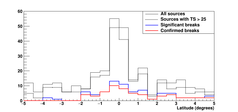
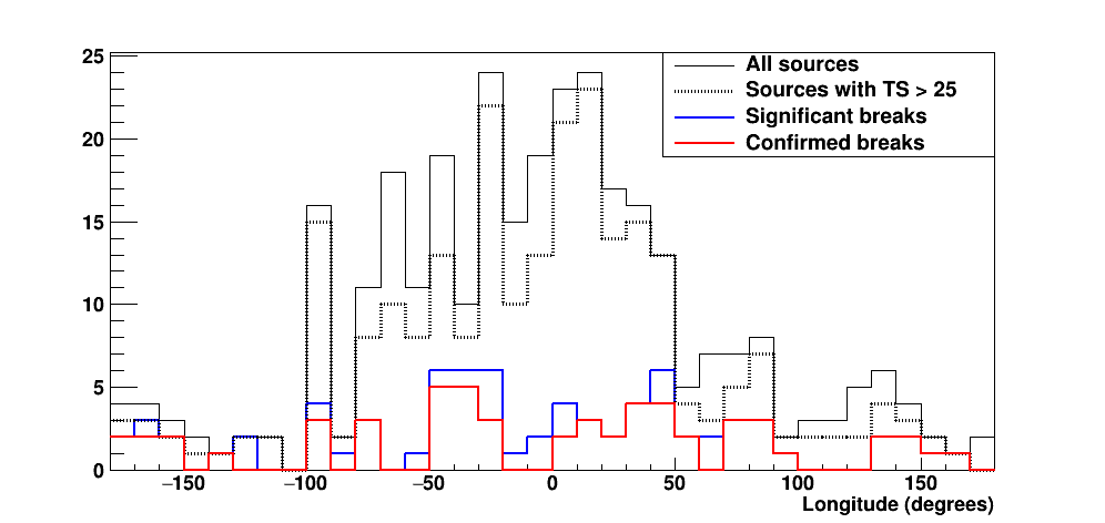
Figure 3: Latitude (top) and longitude (bottom) distributions of the 311 sources selected (black line), the 247 sources with $TS>25$ in our pipeline (black dashed line), the 77 sources with significant breaks (blue line) and the 56 confirmed cases by our studies of systematics (red line).

Table 5: Summary of source classes

Source class	Analyzed	Confirmed
Supernova remnant (SNR)	23	13
Pulsar wind nebulae (PWN)	4	2
Supernova remnant / Pulsar wind nebula (SPP)	37	6
Star-forming region (SFR)	1	1
Unknown (UNK)	31	4
Binary/High-mass binary (BIN/HMB)	5	4
Unidentified (UNID)	210	26

Note. — For the source classes SNR, PWN, SPP, SFR, BIN and HMB, we add both the firm identifications reported in the 4FGL catalog as well as the associations (capital and lower case letters as seen in Column 6 of Table 8)

4 Discussion

4.1 Population study

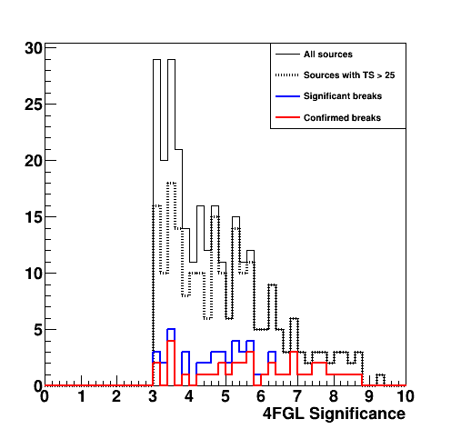
Figure 4: Distribution of the 4FGL significance between 300 MeV and 1 GeV for the 311 sources selected (black line), the 247 sources with $TS>25$ in our pipeline (black dashed line), the 77 sources with significant breaks (blue line) and the 56 confirmed cases by our studies of systematics (red line).

We detected 56 4FGL $\gamma$-ray sources showing a significant energy break in their spectrum between 50 MeV and 1 GeV confirmed by our studies of systematics. As can be seen in Figure 3, the distribution of sources showing a significant break in their low-energy spectrum is more uniform in both latitude and longitude than the parent distribution even if there remains a peak at latitude 0 and in the Galactic Ridge.
The sources that we detect significantly with our analysis (${\rm TS}>25$) follow the same trend except for the region at $\sim 300^{\circ}$ longitude which contains more faint sources than the other regions of the plane. Figure 4 clearly shows that the sources that we do not detect with ${\rm TS}>25$ in our pipeline have predominantly low significance in the 4FGL catalog in the 300 MeV – 1 GeV energy band, which is reassuring. However, there is no correlation between the significance value in the 4FGL catalog and the detection of a break with our pipeline. It can be seen in this same Figure since the distribution for the sources presenting a significant break is uniform.

The association summary is given in Table 5 and is illustrated by the pie charts in Figure 5. Out of 311 candidates, 210 are unidentified, representing 67.5% of the sources analyzed. It is striking to see that only 26 UNIDs show a spectral break confirmed with our systematic studies (which represents 46.4% of the sources with significant breaks). The 30 remaining candidates out of 56 confirmed cases present an association reported by the 4FGL Catalog listed in Table 6.
On the other hand, the fraction of sources associated with supernova remnants (SNRs) increases from 7.4% (23 out of 311 sources) to 23.2% (13 out of 56 sources). This makes SNRs the dominant class of sources with significant low-energy spectral break. Similarly, the fraction of sources associated with binaries increases from 1.6% (5 out of 311) to 7.1% (4 out of 56), showing that almost all binaries except 4FGL J1826.2$-$1450 (also known as LS 5039), show a significant spectral break. Despite their small fractions, binaries could contribute significantly to our population of sources with low-energy spectral breaks; however it should be noted here that the spectral analysis is performed over 8 years and these sources often present variable $\gamma$-ray emission. A more thorough analysis of these sources would need to be done. Finally, only one star-forming region is analyzed (and confirmed) which prevents us from drawing a firm conclusion on this source class.
Figure 6 illustrates the distribution over the sky of the 56 4FGL $\gamma$-ray sources showing a significant energy break. The lack of these sources at latitude smaller than $-2^{\circ}$ appears clearly. One can also note a large fraction of unidentified sources at longitude comprised between $-50^{\circ}$ and $50^{\circ}$. These sources are part of the large fraction of 4FGL unassociated sources located less than $10^{\circ}$ away from the Galactic plane with a wide latitude extension hard to reconcile with those of known classes of Galactic $\gamma$-ray sources.

Looking now at the spectral parameters of the 56 confirmed sources, the distribution of the energy of the breaks detected by our analysis is relatively uniform between 70 MeV and 700 MeV, with no breaks detected below and above this energy interval (as a direct consequence of the energy interval analyzed here) and a higher proportion of breaks at $\sim$400 MeV as illustrated by Figure 7. Interestingly, no low energy spectral breaks ($<140$ MeV) are detected for the 13 sources associated with SNRs. As can be seen on the top panel of this Figure, the large error bars on this parameter prevent us from drawing any firm conclusion or even rejecting any candidate by a comparison with the standard value expected for proton-proton interaction indicated by the green line. On the other hand, there is a trend concerning the distributions of $\Gamma_{1}$ with a peak at $\sim 0.2$ and $\sim 1.0$. The peak at 0.2 is expected by proton-proton interaction (as indicated by the green line presenting the results of the simulations carried in Appendix A) but the peak at 1 is not predicted, though it is present for a large number of SNRs interacting with MCs. It might be due to some confusion by the Galactic and isotropic diffuse background. A double-peaked distribution is also visible in Figure 8 for $\Gamma_{2}$ at $\sim 2.1$ and $\sim 3.6$. For this parameter, the distribution restricted to SNRs contains a single peak at $\sim 2.1$. Looking now at the distribution of $\Gamma_{2}-\Gamma_{1}$ in Figure 8 (right), a peak at $\sim 0.9$ is highly pronounced for SNRs. This tends to show that the values obtained on $\Gamma_{2}$ and $\Gamma_{2}-\Gamma_{1}$ could be used in the future to probe the type of particles radiating in a $\gamma$-ray source.

Table 6: Candidates with firm associations reported in the 4FGL Catalog

4FGL Name	Assoc1	Assoc2
4FGL J0222.4+6156e	W 3	HB 3 field
4FGL J0240.5+6113	LS I +61 303
4FGL J0500.3+4639e	HB 9
4FGL J0540.3+2756e	Sim 147
4FGL J0617.2+2234e	IC 443
4FGL J0634.2+0436e	Rosette	Monoceros field
4FGL J0639.4+0655e	Monoceros
4FGL J0904.7$-$4908	1RXS J090505.3$-$490324
4FGL J1008.1$-$5706	1RXS J100718.2$-$570335
4FGL J1018.9$-$5856	1FGL J1018.6$-$5856	FGES J1036.3$-$5833 field
4FGL J1045.1$-$5940	Eta Carinae	FGES J1036.3$-$5833 field
4FGL J1442.2$-$6005	SNR G316.3$-$00.0
4FGL J1514.2$-$5909e	MSH 15$-$52
4FGL J1552.9$-$5607e	MSH 15$-$56
4FGL J1601.3$-$5224	SNR G329.7+00.4
4FGL J1633.0$-$4746e	HESS J1632$-$478
4FGL J1801.3$-$2326e	W 28
4FGL J1813.1$-$1737e	HESS J1813$-$178
4FGL J1839.4$-$0553	NVSS J183922$-$055321	HESS J1841$-$055 field
4FGL J1852.4+0037e	Kes 79
4FGL J1855.9+0121e	W 44
4FGL J1857.7+0246e	HESS J1857+026
4FGL J1911.0+0905	W 49B
4FGL J1923.2+1408e	W 51C
4FGL J1934.3+1859	SNR G054.4$-$00.3
4FGL J2021.0+4031e	gamma Cygni	Cygnus Cocoon field
4FGL J2028.6+4110e	Cygnus X Cocoon
4FGL J2032.6+4053	Cyg X$-$3	Cygnus Cocoon field
4FGL J2045.2+5026e	HB 21
4FGL J2056.4+4351	1RXS J205549.4+435216

Note. — Columns 2 and 3 are derived from the Assoc1 and Assoc2 columns of the 4FGL Catalog. The latter provides an alternate designation or an indicator as to whether the source is inside an extended source.

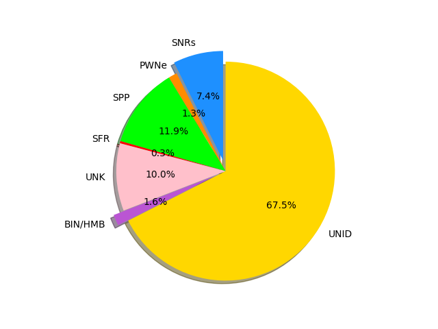
Figure 5: Pie charts showing the classes of sources analyzed (Left) and those for which a significant break is detected (Right). The class names are those used in the 4FGL catalog: SNR stands for Supernova remnant, PWN for pulsar wind nebula, SFR for star-forming region, BIN for binary, HMB for high-mass binary. The designation SPP indicates potential association with SNR or PWN. The UNK class includes low-latitude blazar candidates of uncertain type associated solely via the Likelihood-Ratio (LR) method.

Figure 6: Distribution of sources in Galactic coordinates. Light gray markers indicate the 311 sources analyzed in this paper. Coloured markers indicate the position of the 56 sources for which a significant break is detected: yellow for UNIDs, blue for SNRs, orange for PWNe, green for SPPs, red for SFR, pink for UNKs and purple for BIN/HMB. The boundary of the latitude selection is $5^{\circ}$.

Figure 7: Break energy for the 56 sources confirmed by our studies of systematics (black line) and for the identified SNRs and/or crushed molecular clouds (dotted line, see Section 4.2). The green line indicates the value of the break energy obtained using simulations based on the $naima$ package for a proton injection index of 2.0 and the two green dotted-dashed lines indicate the one sigma confidence interval derived (more details in the Appendix A). (Top) Individual values; (Bottom) Corresponding histograms.

4.2 Supernova remnants and molecular clouds

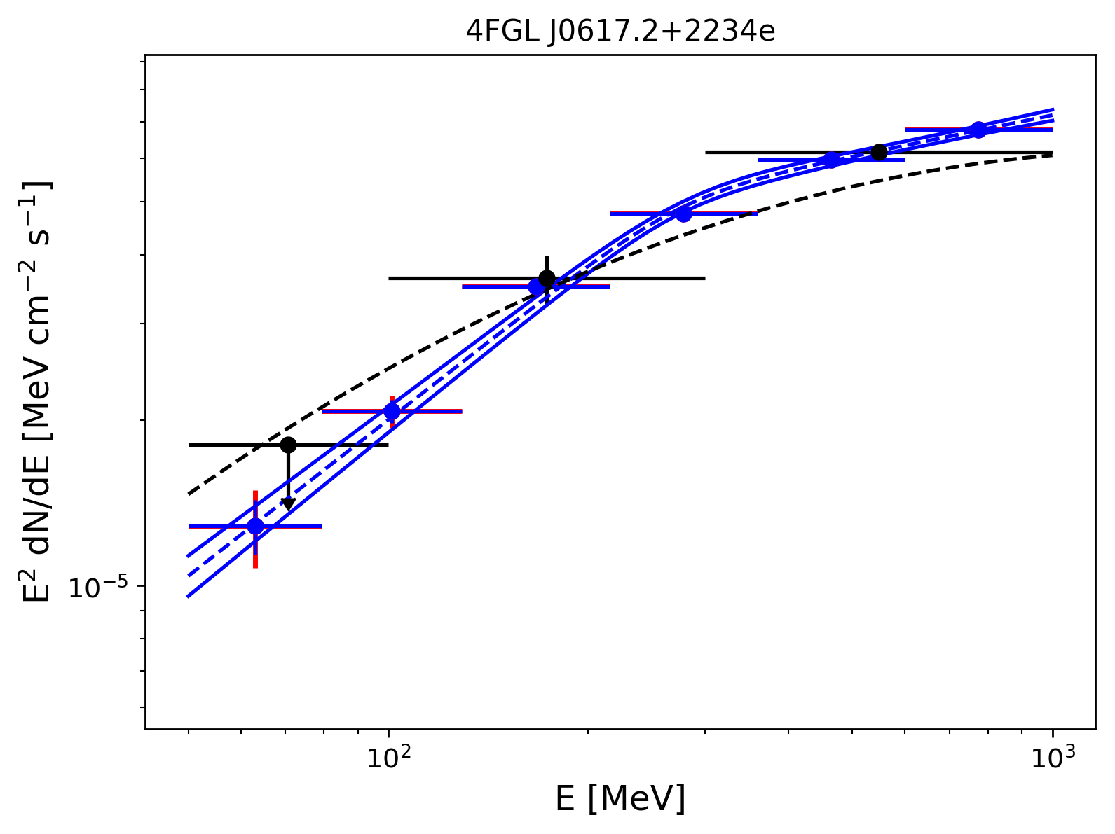
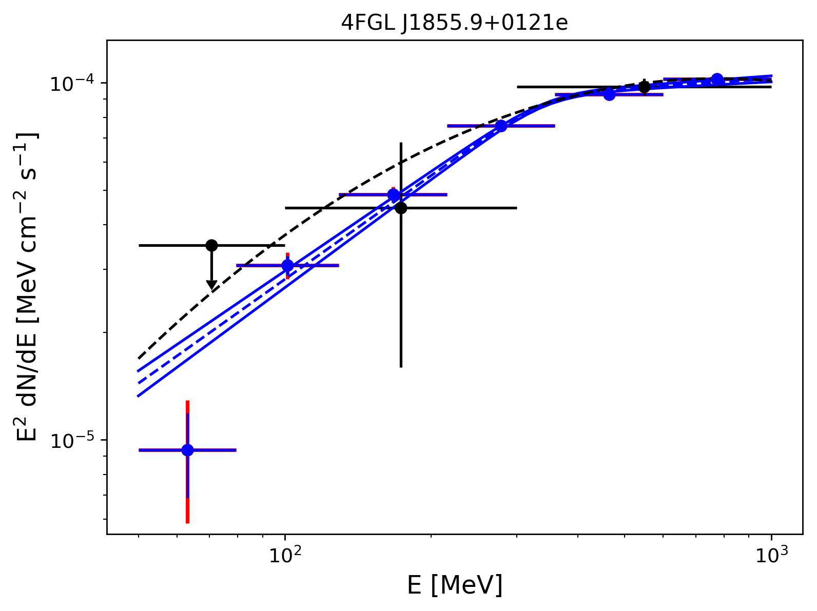
Figure 9: LAT residual TS maps in equatorial coordinates and significance units (left) and spectral energy distributions (right) of IC 443 (top) and W44 (bottom) between 50 MeV and 1 GeV. In the residual TS maps, all white crosses indicate the 4FGL sources included in the model of the region. For the SEDs, the blue points and butterflies are obtained in this analysis while the black points and dashed line are from the 4FGL catalog. The red lines take into account both the statistical and systematic errors added in quadrature. A 95% C.L. upper limit is computed when the TS value is below 1.

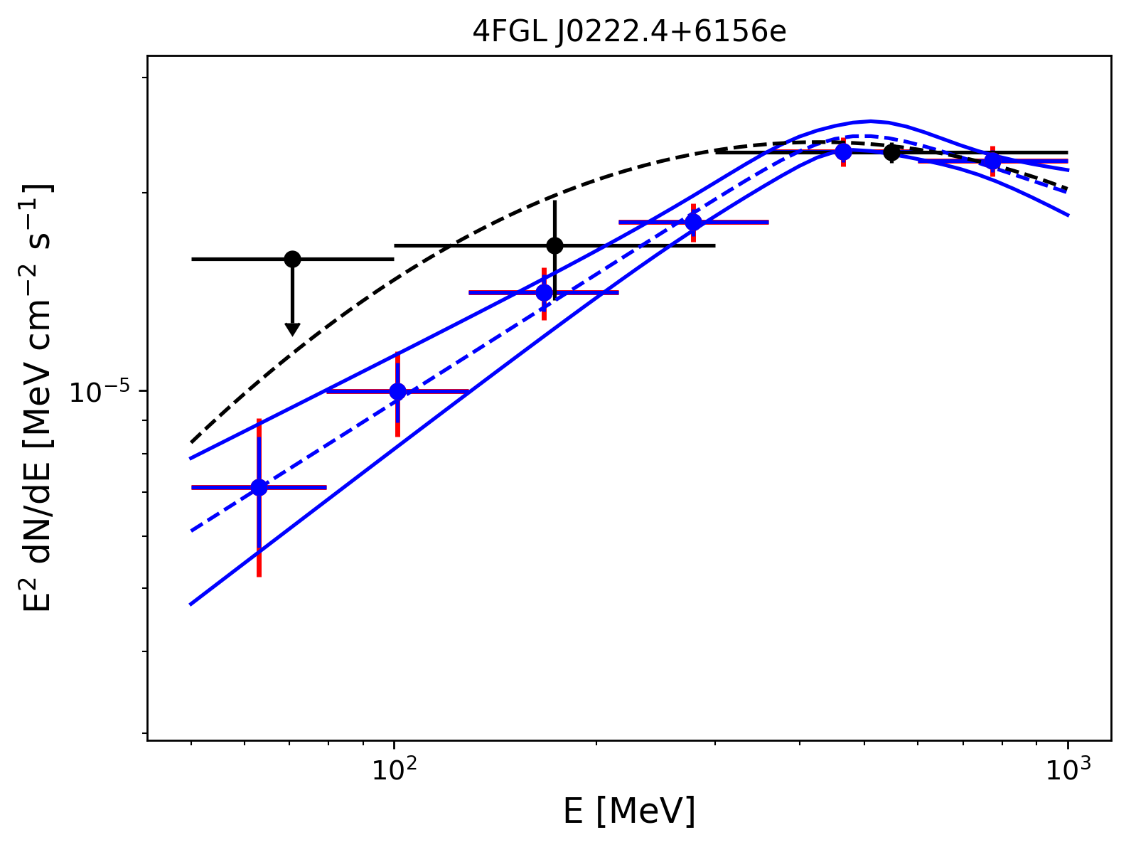
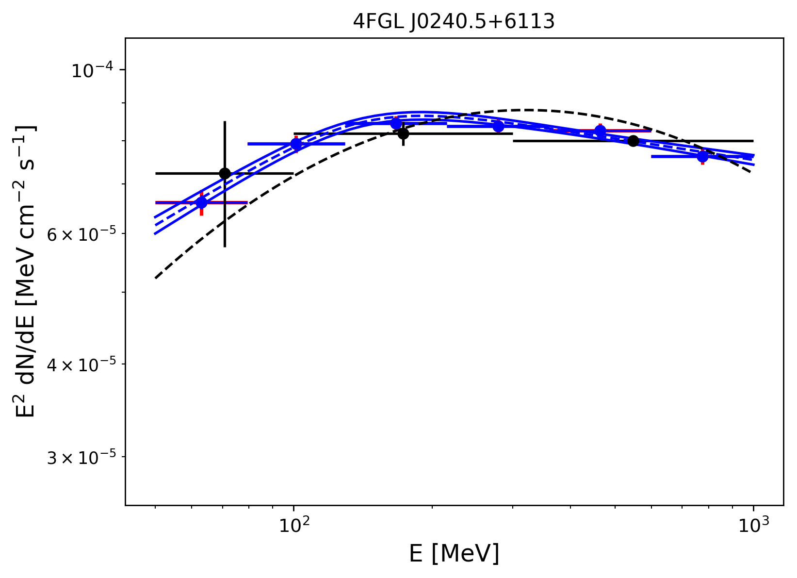
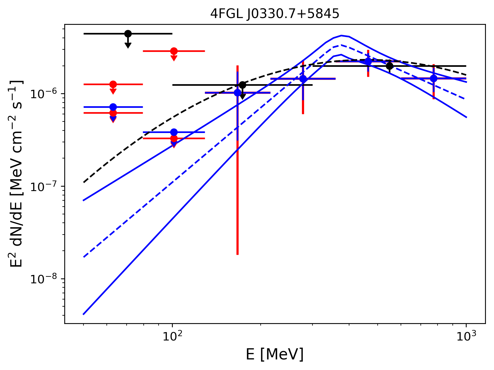
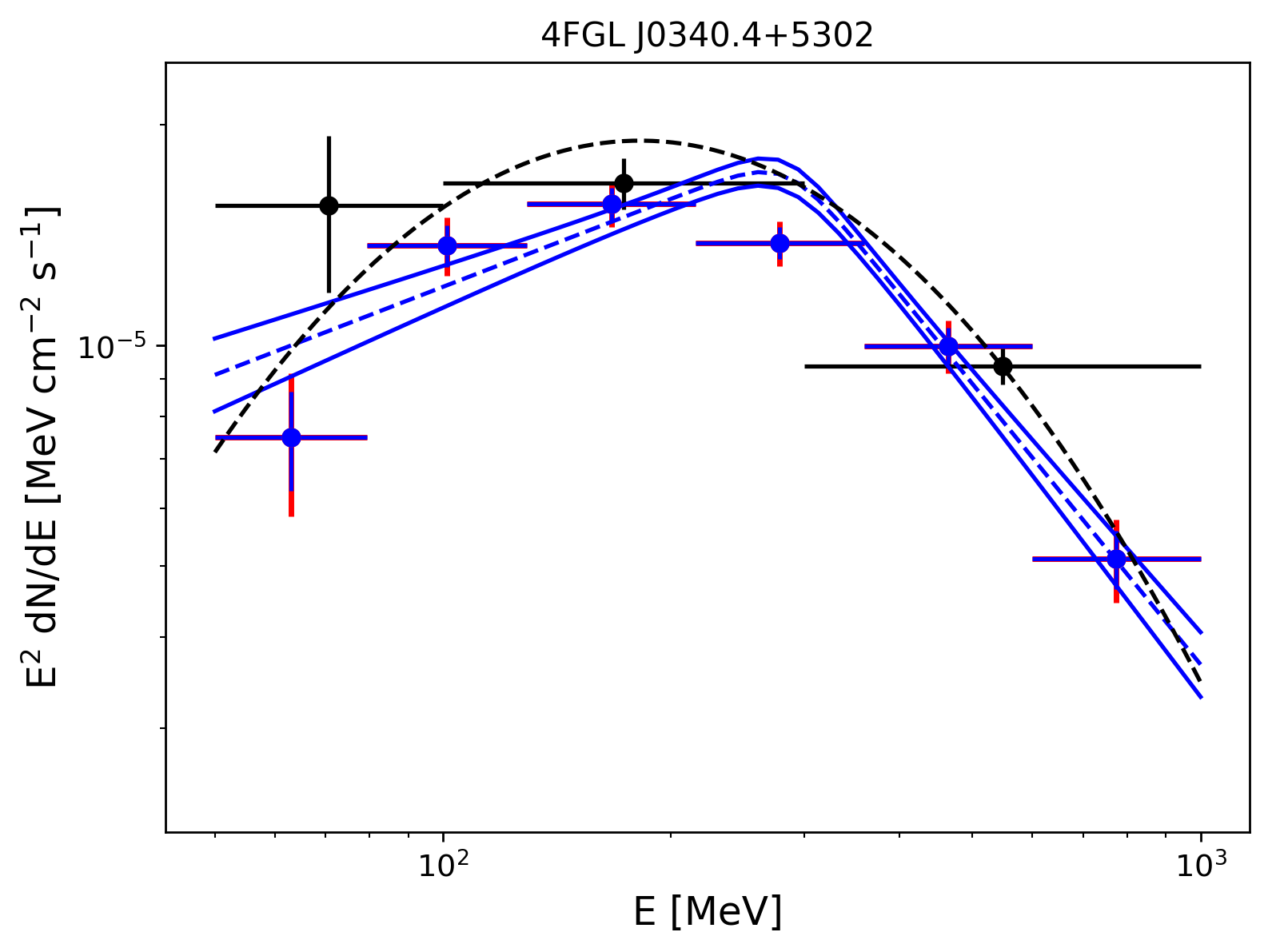
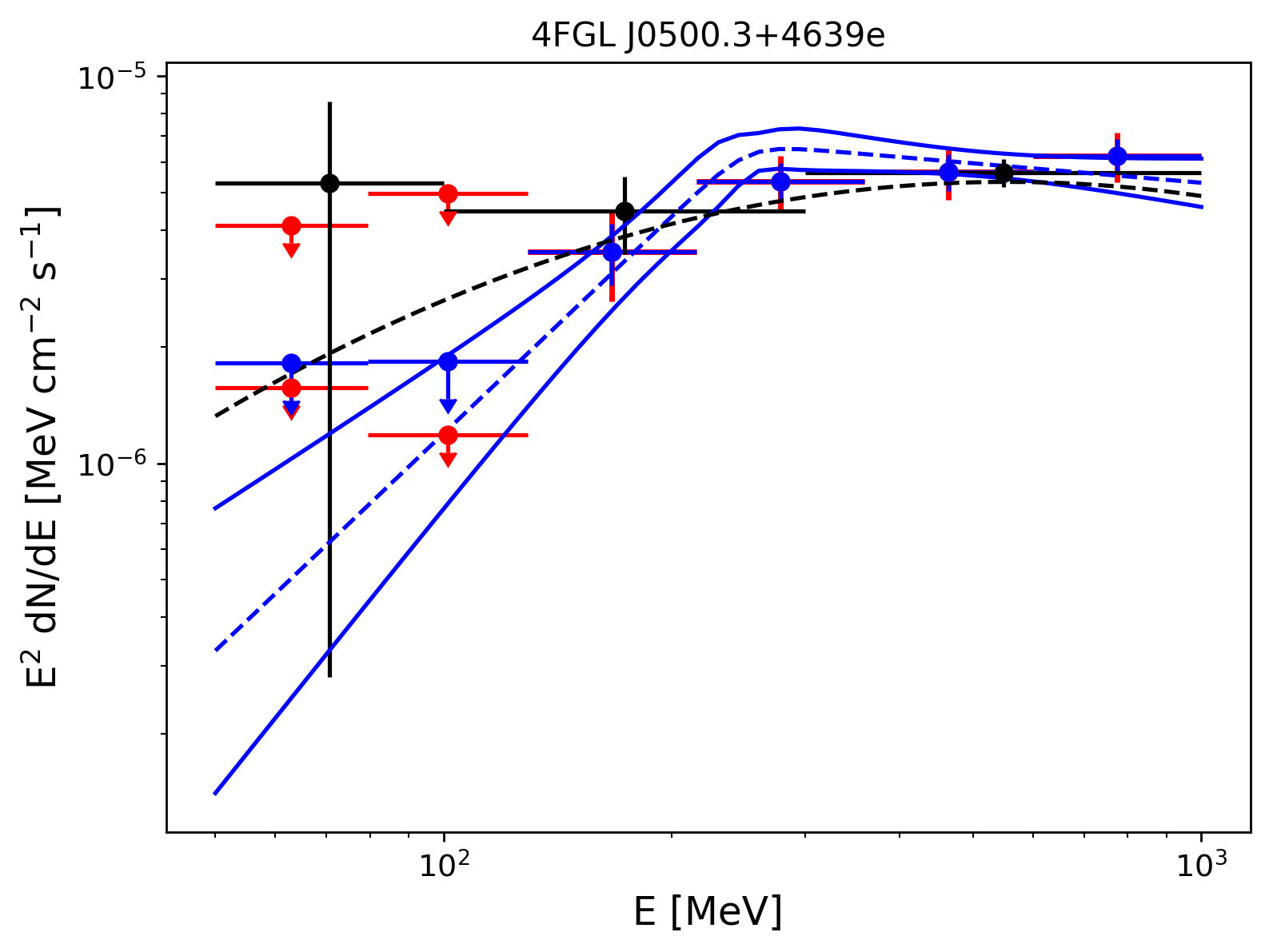
Figure 10: LAT Spectral energy distributions of 4FGL J0222.4+6156e (top left), 4FGL J0240.5+6113 (top right), 4FGL J0330.7+5845 (middle left), 4FGL J0340.4+5302 (middle right), 4FGL J0426.5+5434 (bottom left), 4FGL J0500.3+4639e (bottom right) with the same conventions used in Figure 9.

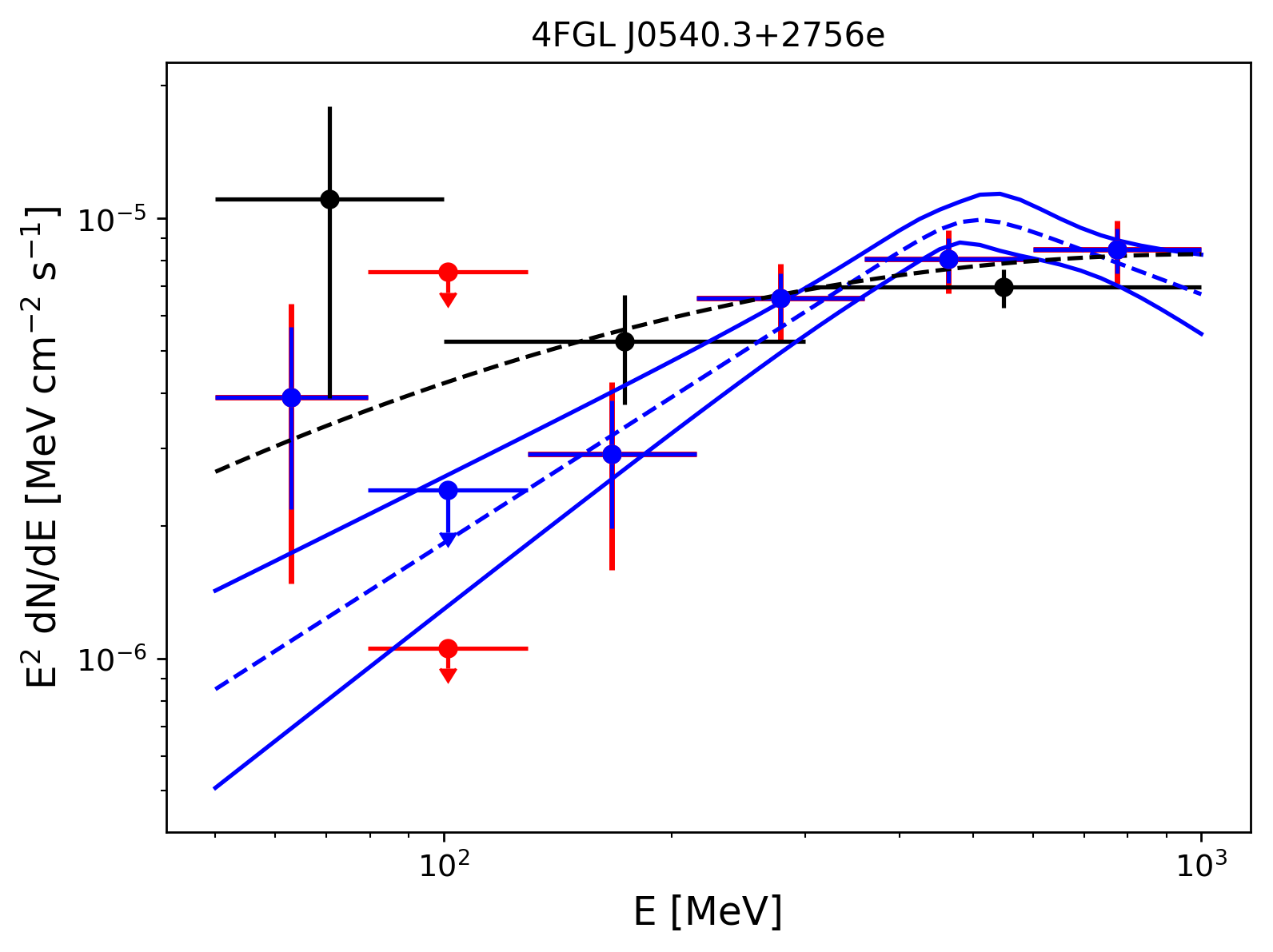
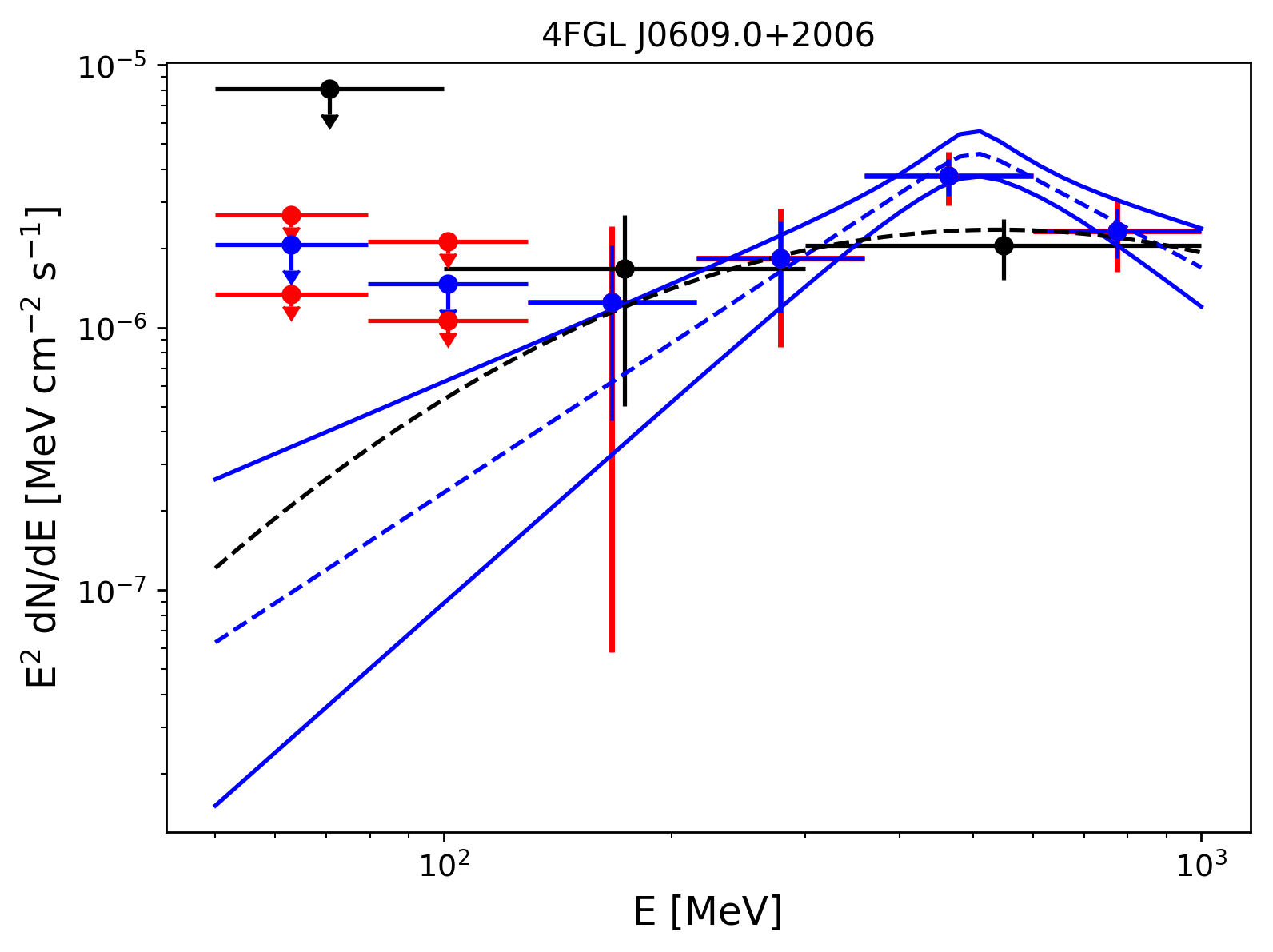
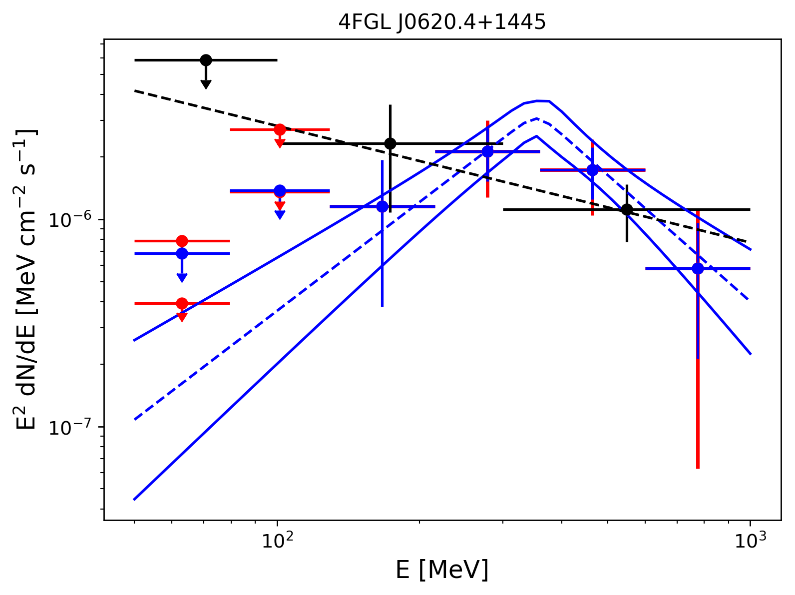
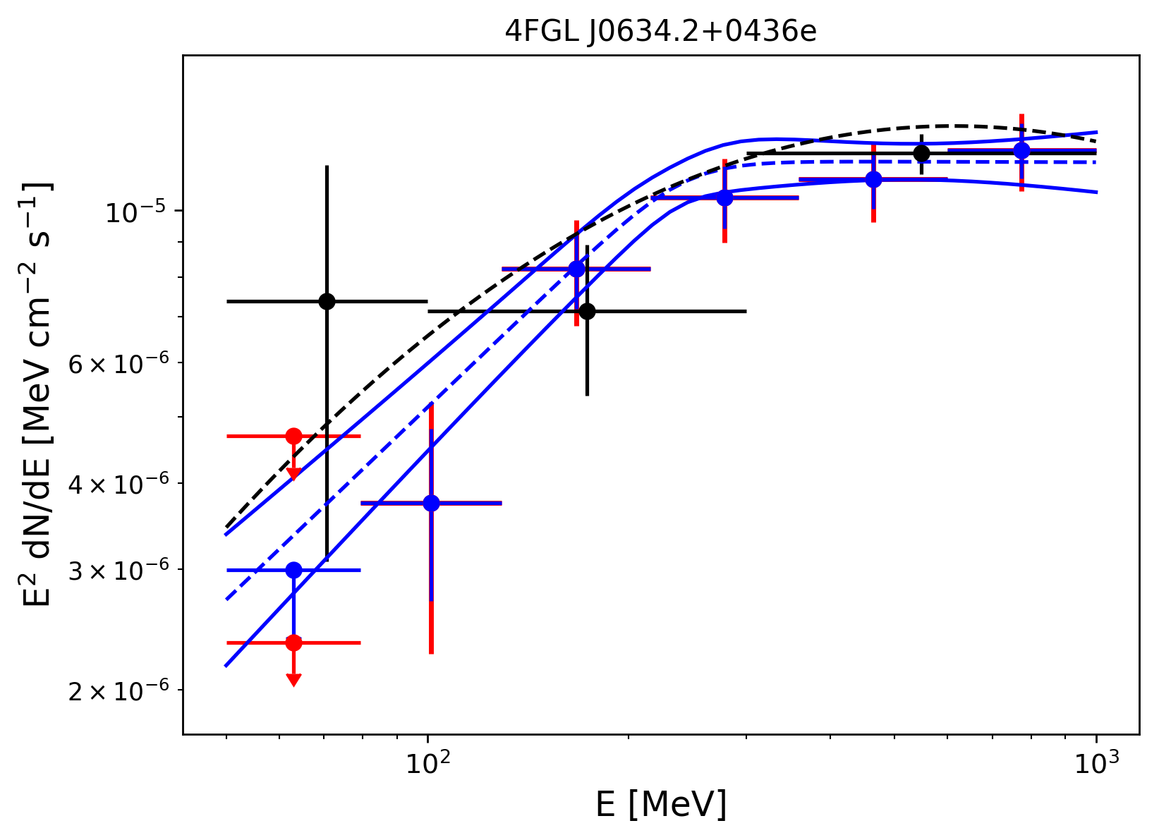
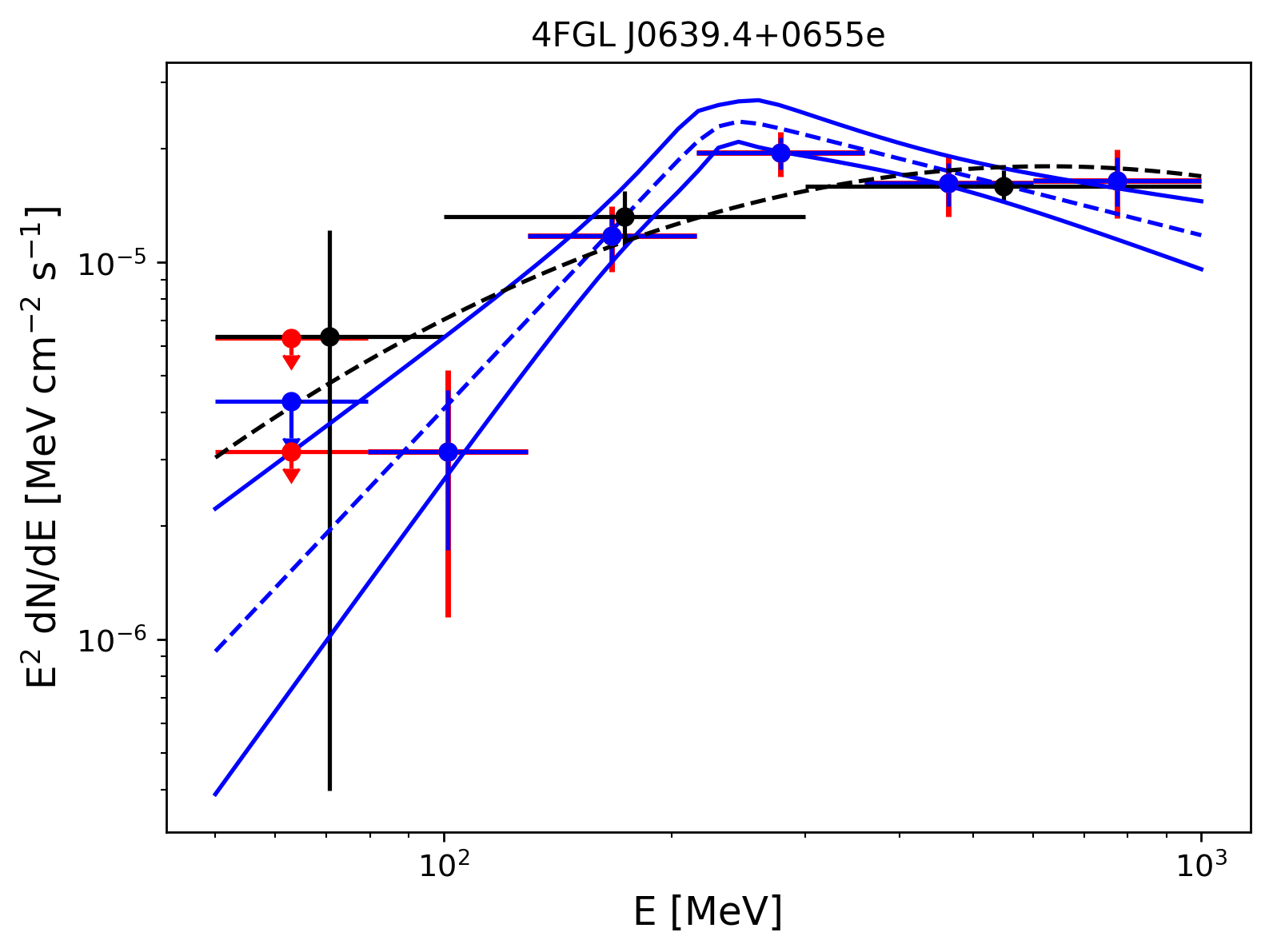
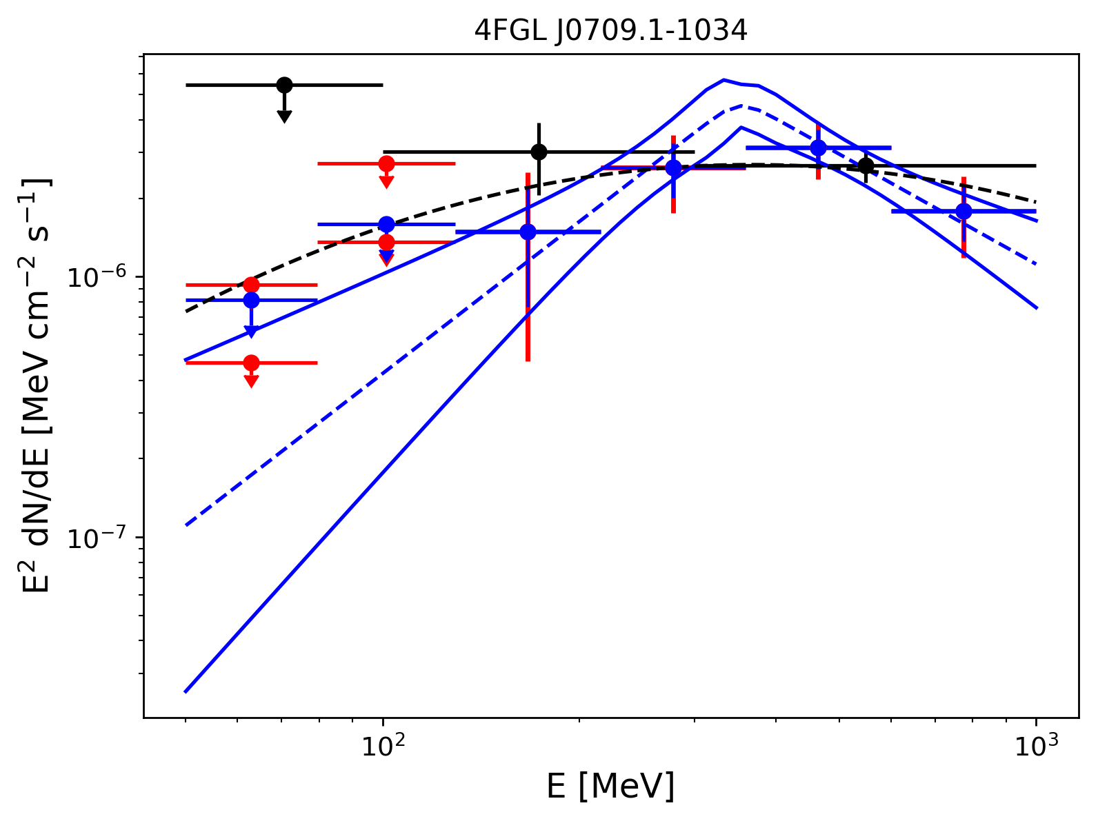
Figure 11: LAT Spectral energy distributions of 4FGL J0540.3+2756e (top left), 4FGL J0609.0+2006 (top right), 4FGL J0620.4+1445 (middle left), 4FGL J0634.2+0436e (middle right), 4FGL J0639.4+0655e (bottom left), 4FGL J0709.1$-$1034 (bottom right) with the same conventions used in Figure 9.

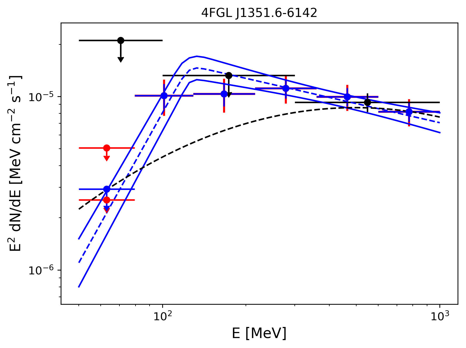
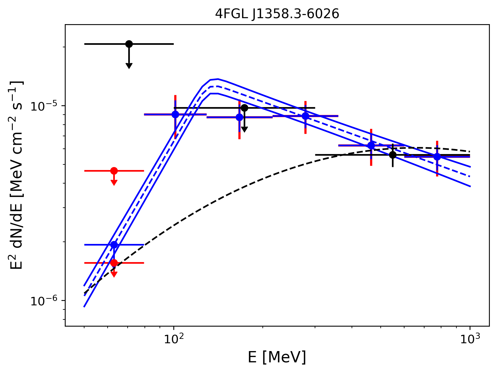
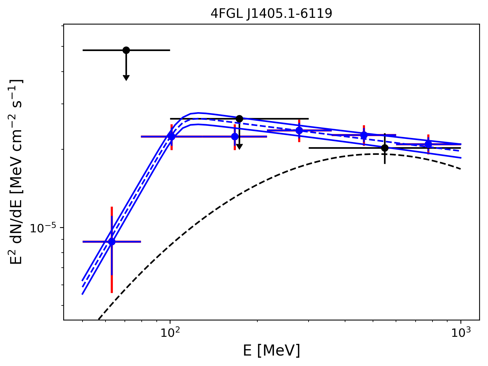
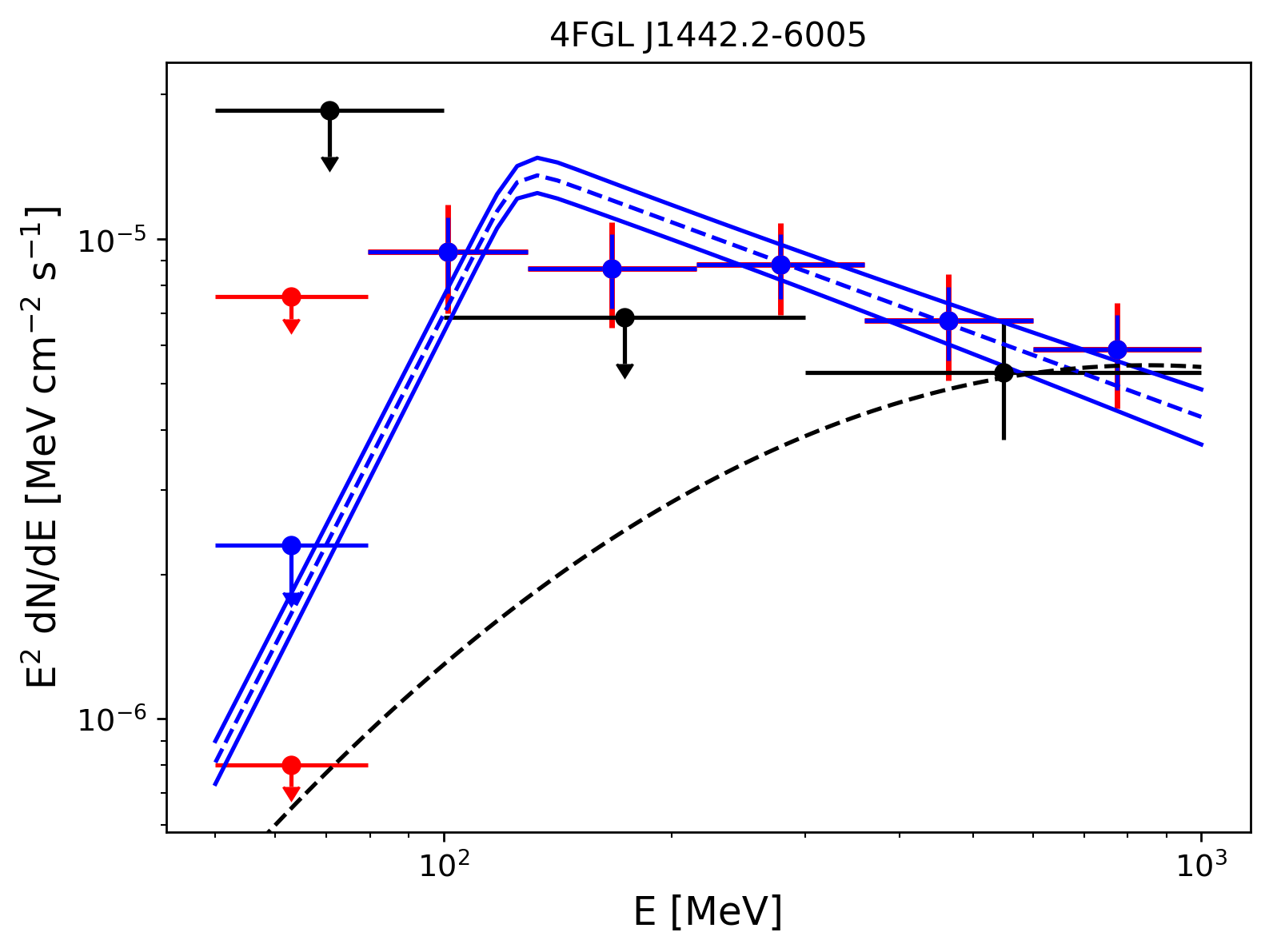
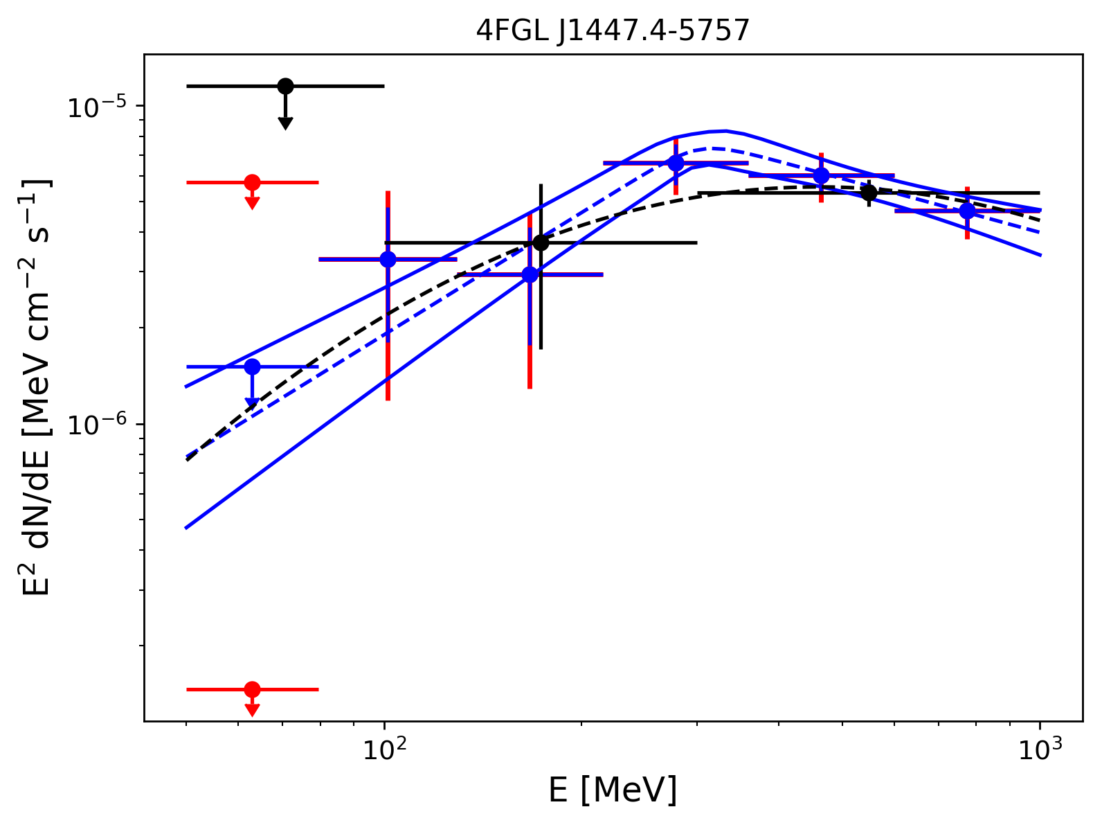
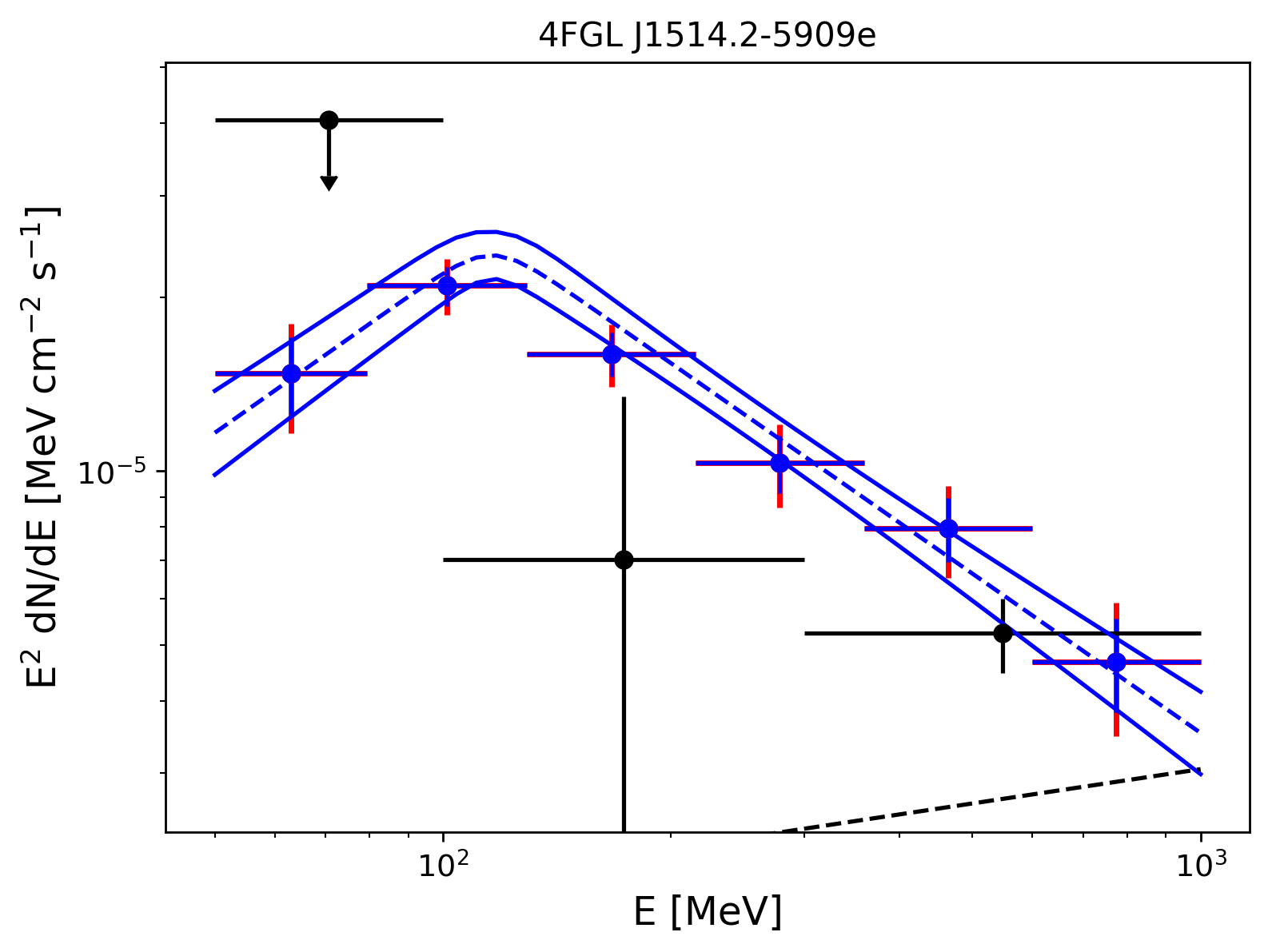
Figure 13: LAT Spectral energy distributions of 4FGL J1351.6$-$6142 (top left), 4FGL J1358.3$-$6026 (top right), 4FGL J1405.1$-$6119 (middle left), 4FGL J1442.2$-$6005 (middle right), 4FGL J1447.4$-$5757 (bottom left), 4FGL J1514.2$-$5909e (bottom right) with the same conventions used in Figure 9.

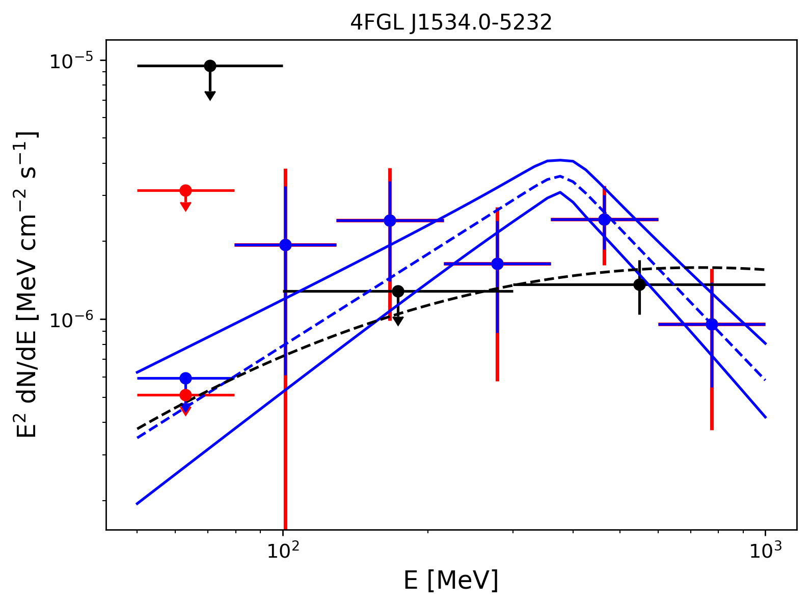
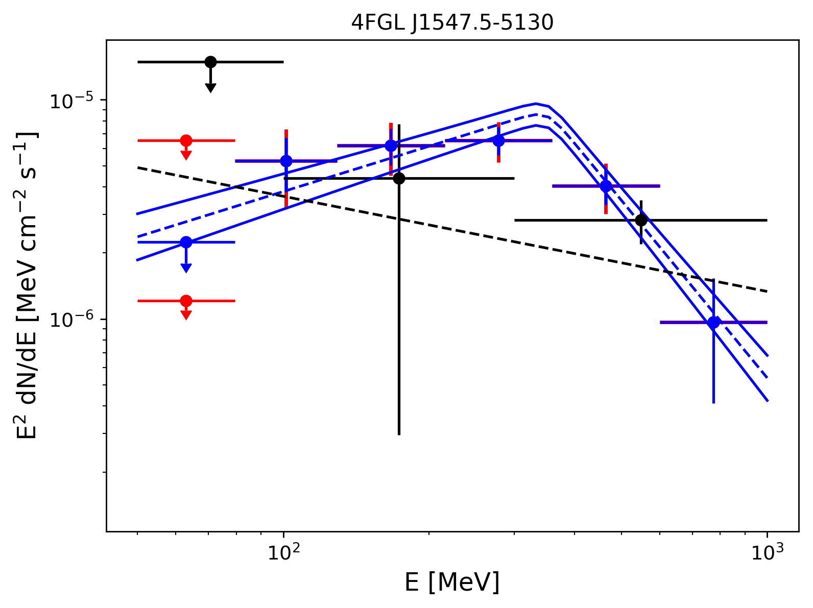
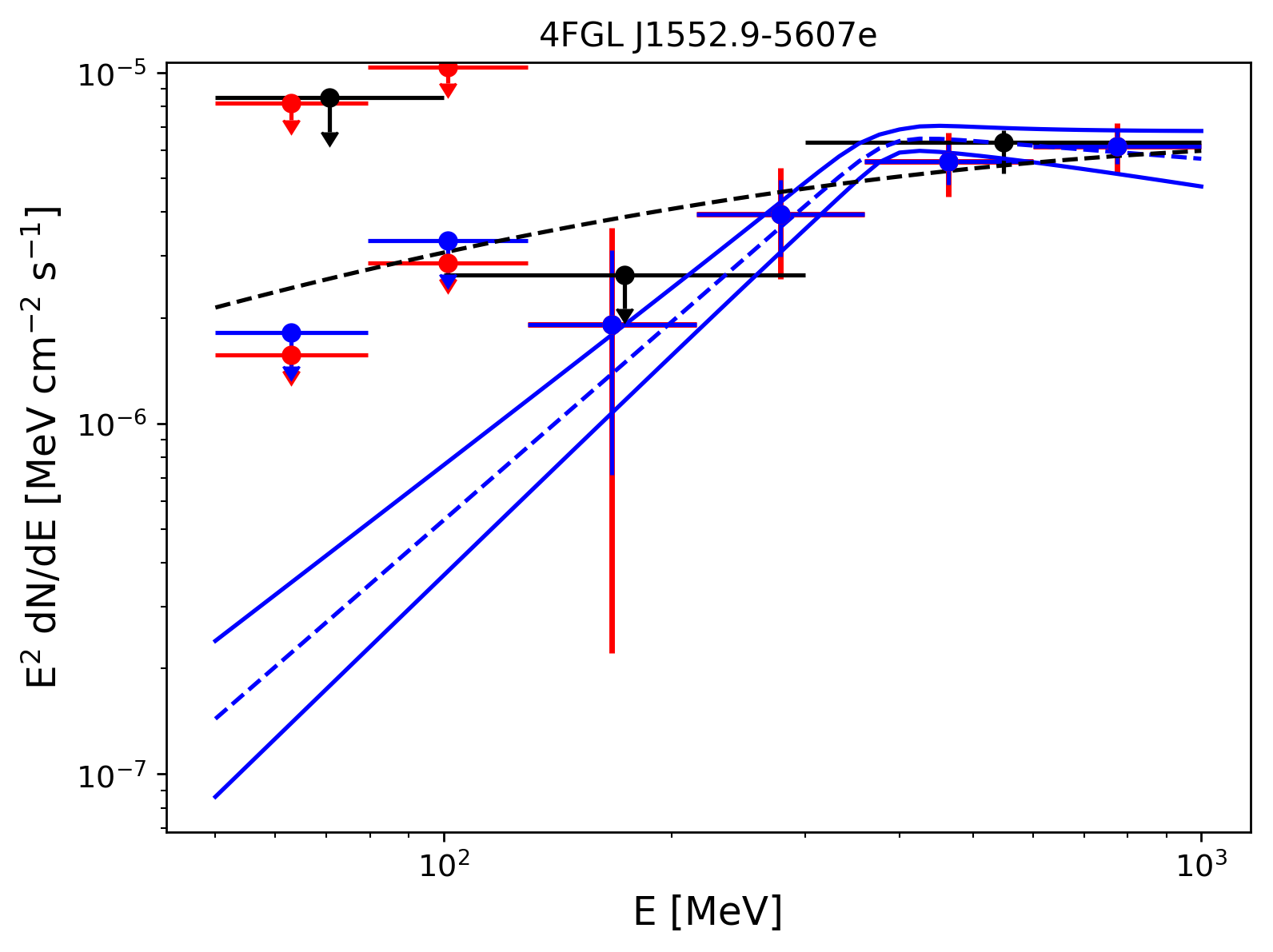
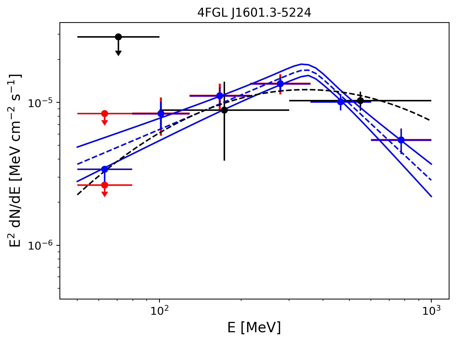
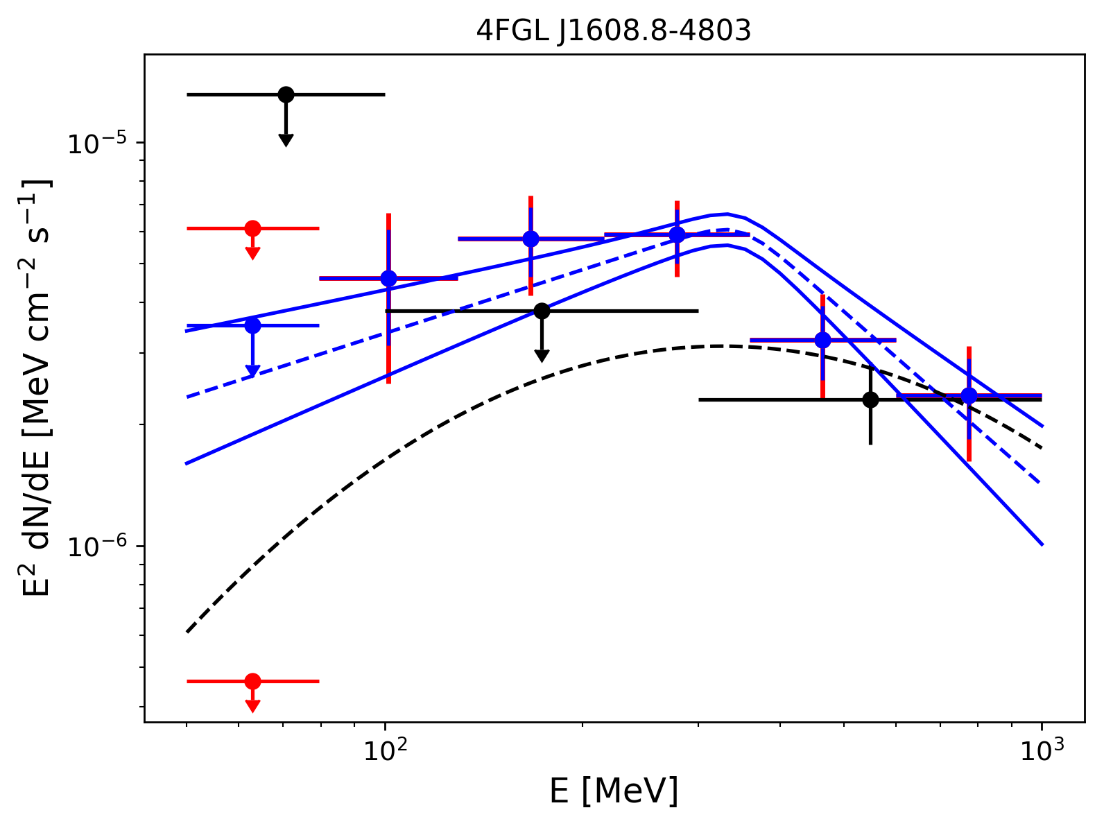
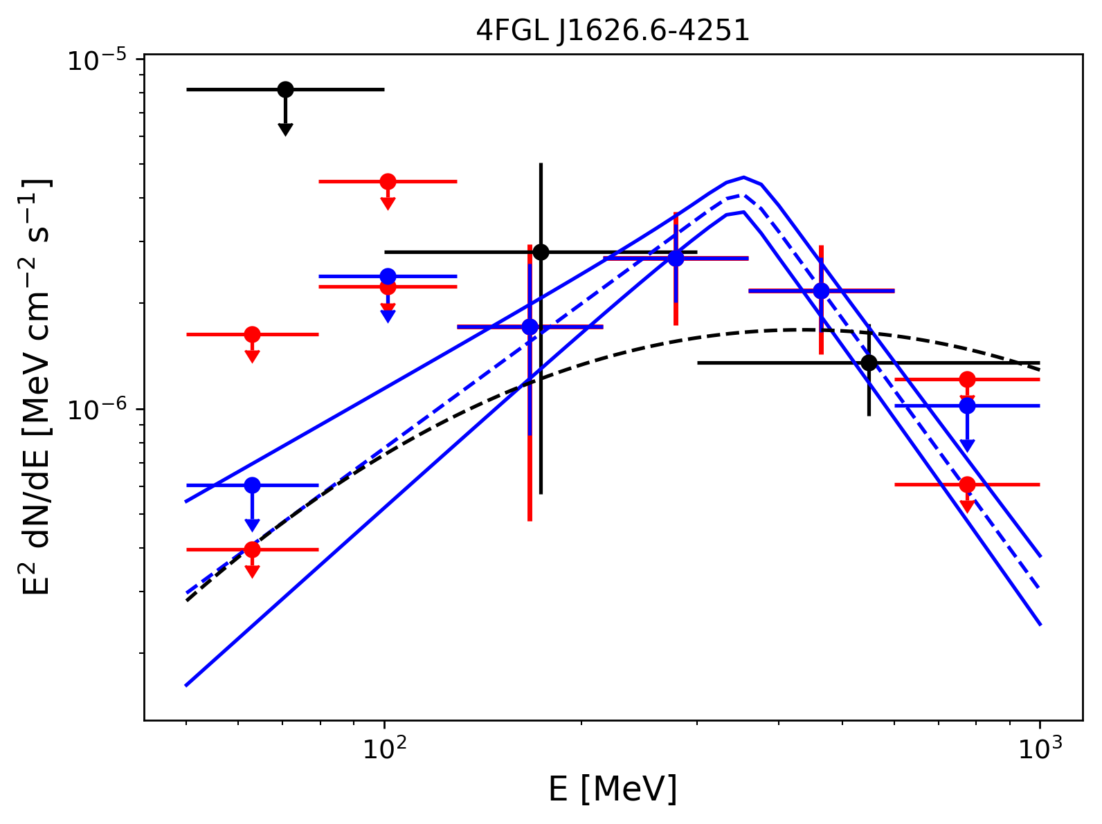
Figure 14: LAT Spectral energy distributions of 4FGL J1534.0$-$5232 (top left), 4FGL J1547.5$-$5130 (top right), 4FGL J1552.9$-$5607e (middle left), 4FGL J1601.3$-$5224 (middle right), 4FGL J1608.8$-$4803 (bottom left), 4FGL J1626.6$-$4251 (bottom right) with the same conventions used in Figure 9.

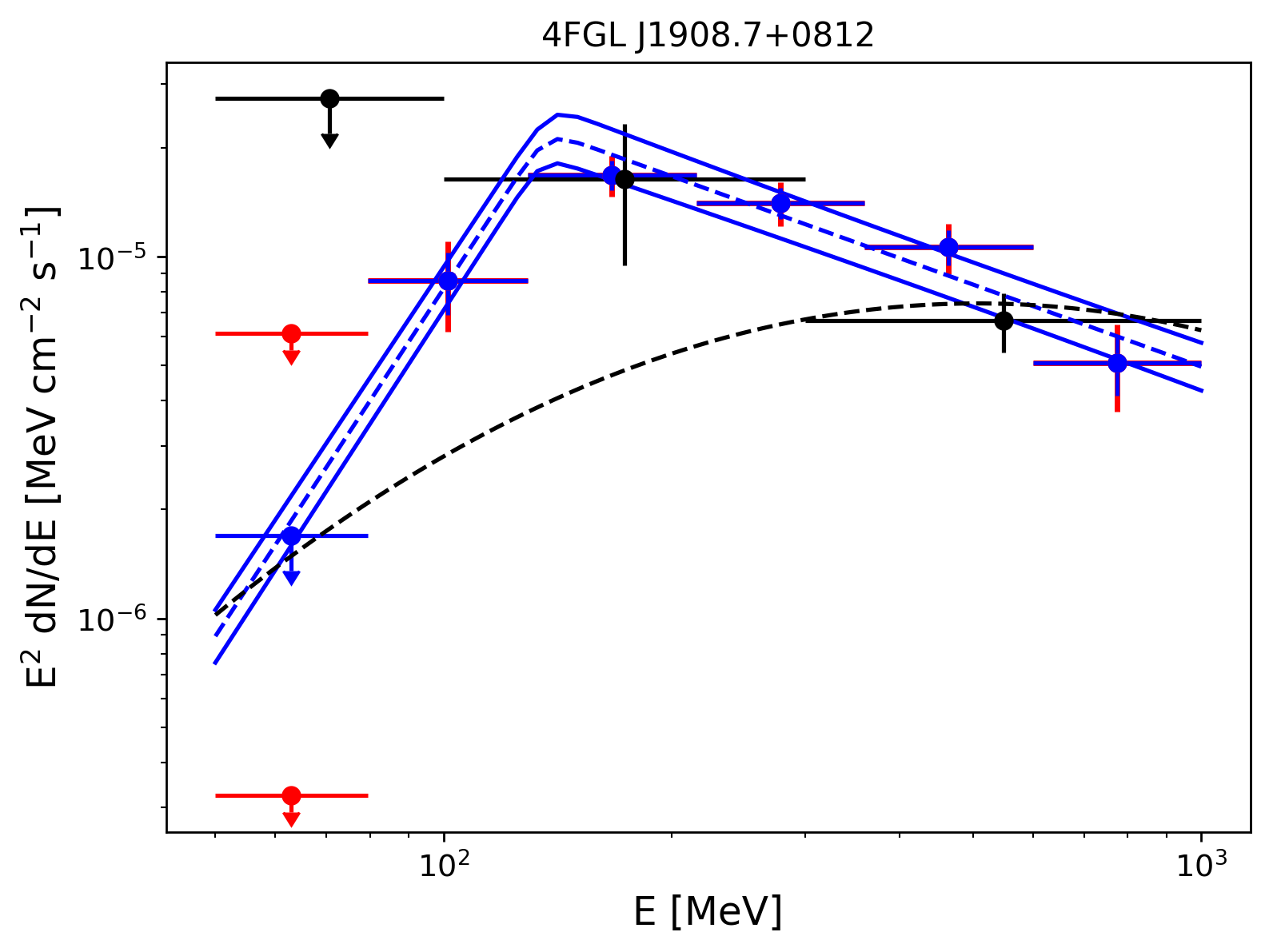
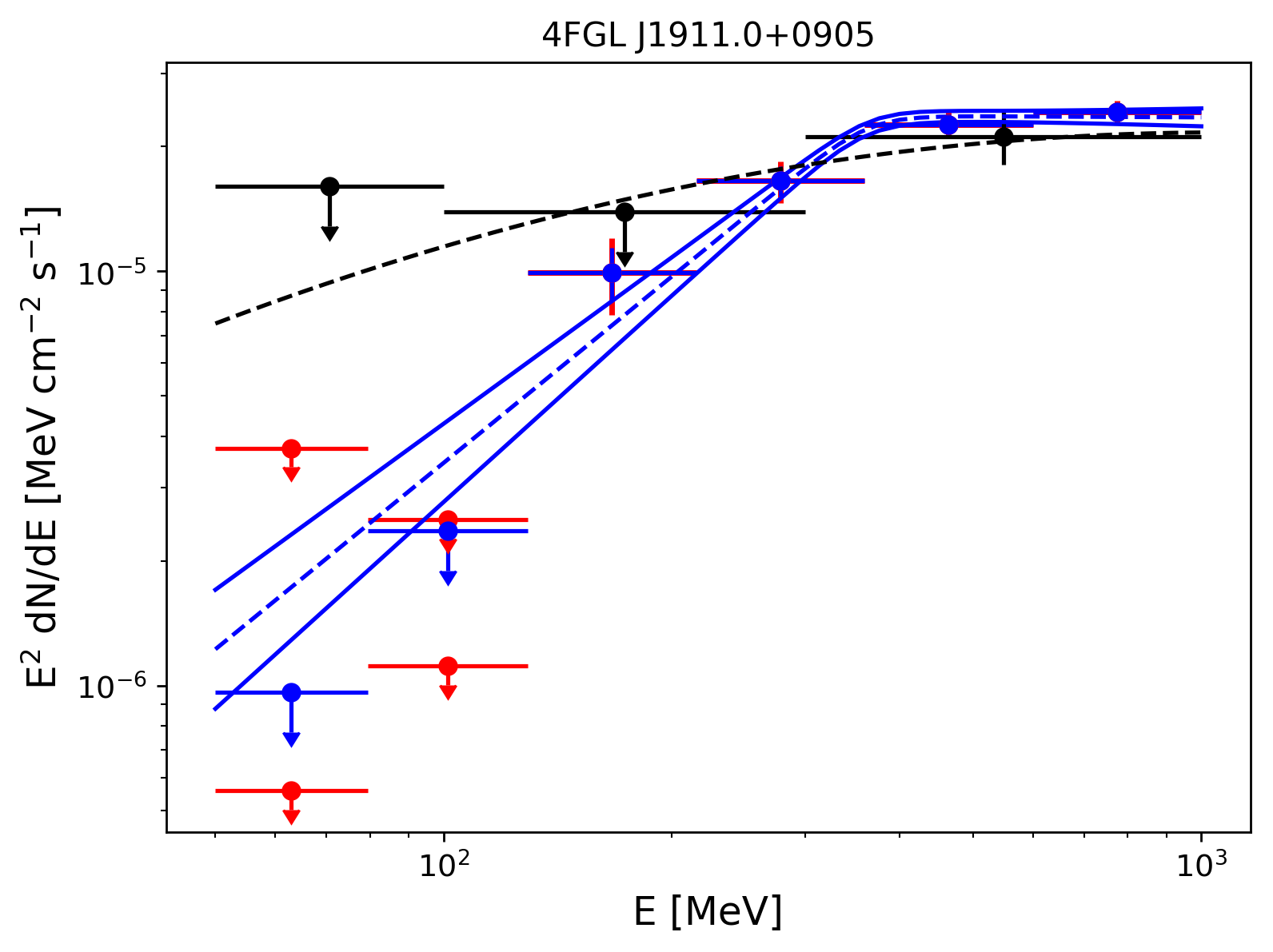
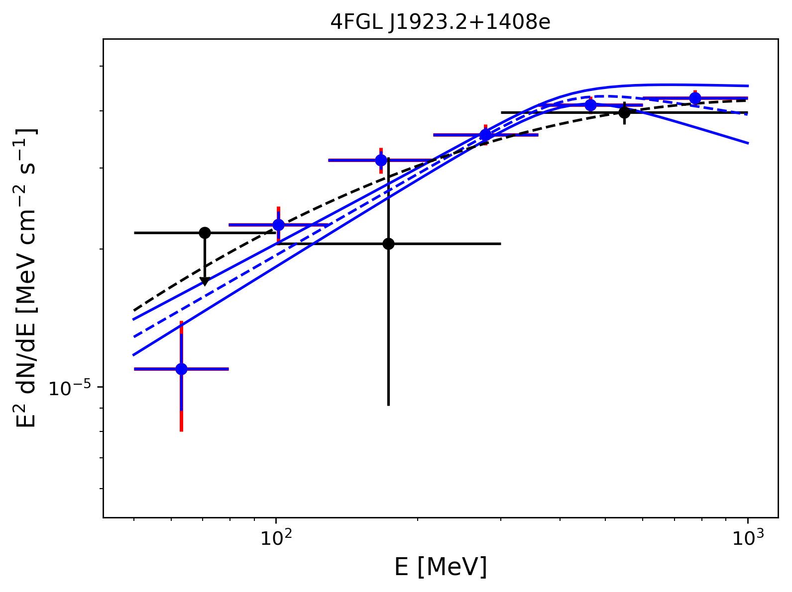
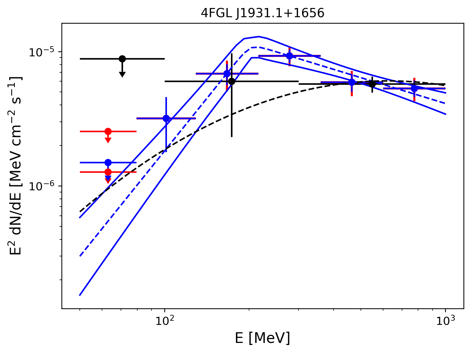
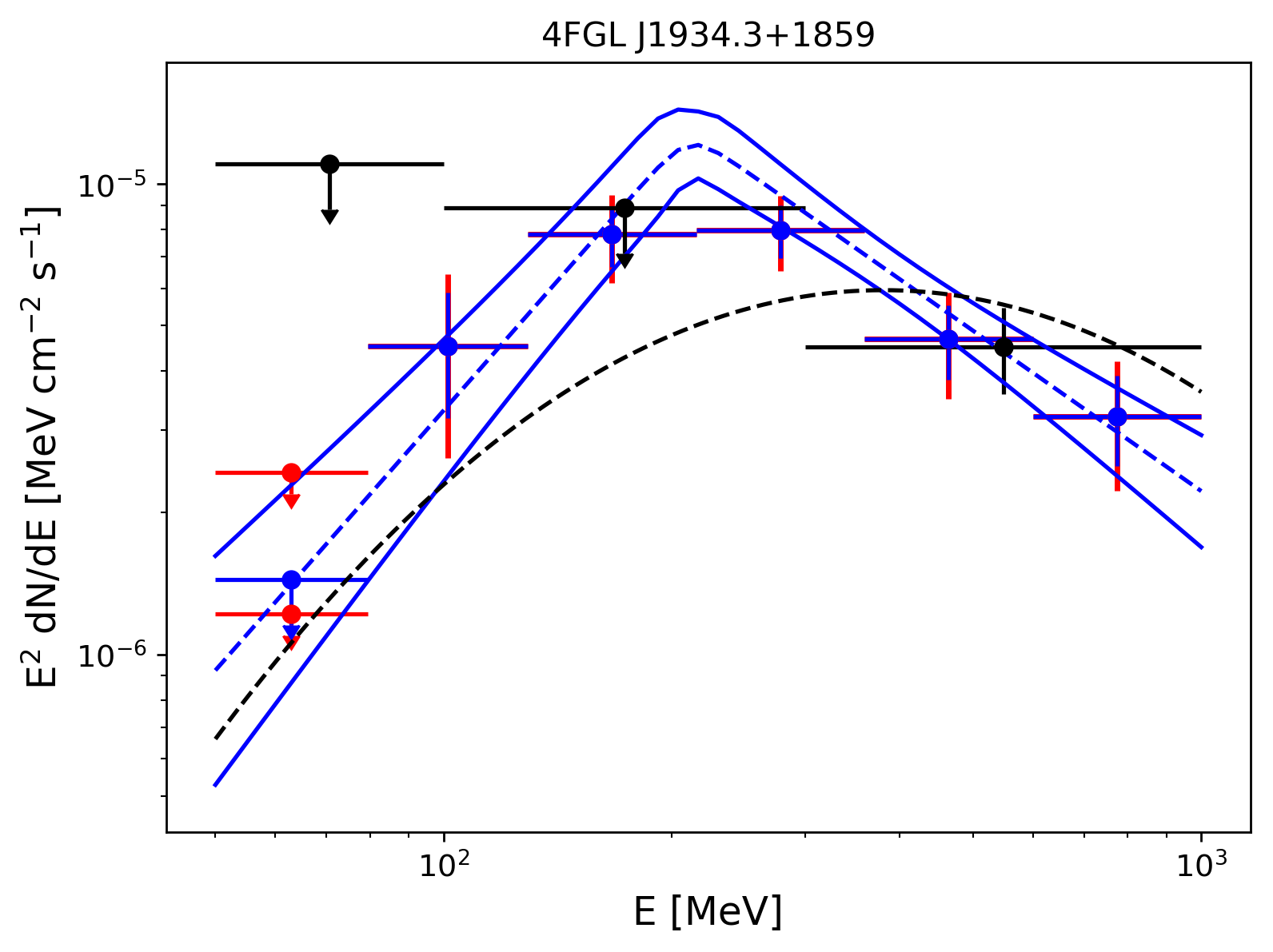
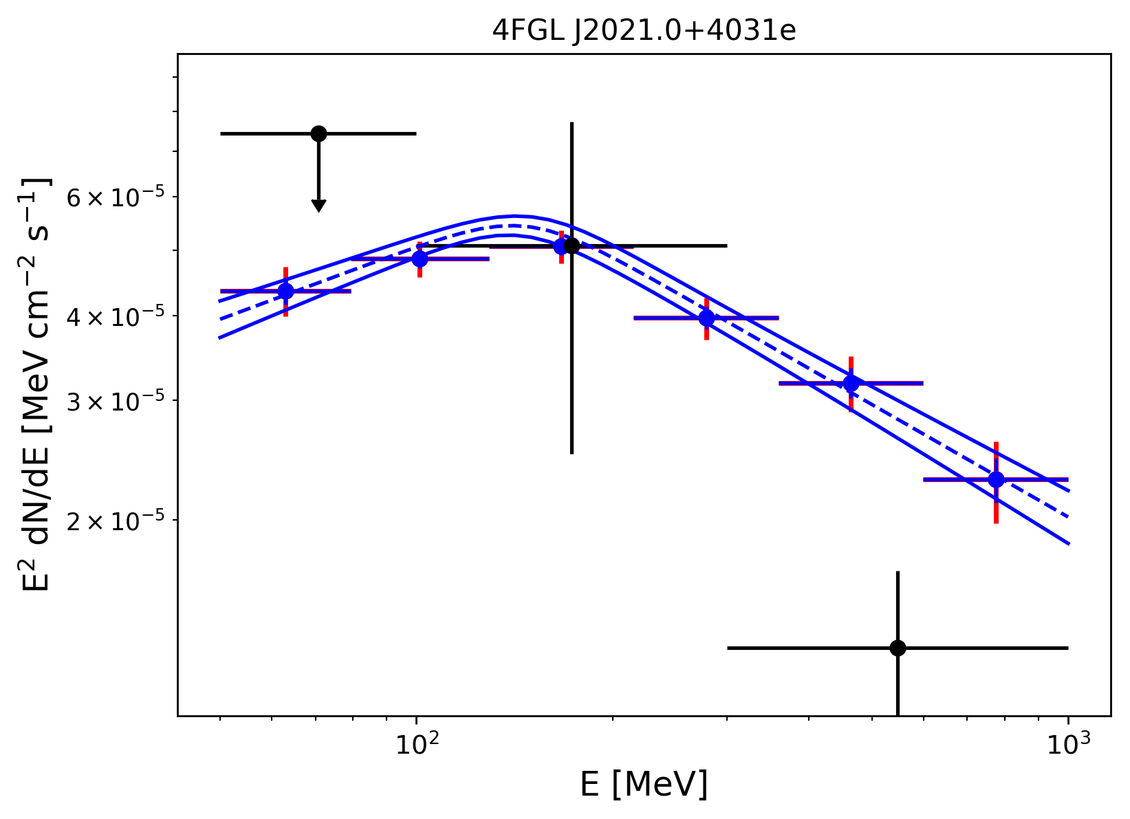
Figure 17: LAT Spectral energy distributions of 4FGL J1908.7+0812 (top left), 4FGL J1911.0+0905 (top right), 4FGL J1923.2+1408e (middle left), 4FGL J1931.1+1656 (middle right), 4FGL J1934.3+1859 (bottom left), 4FGL J2021.0+4031e (bottom right) with the same conventions used in Figure 9.

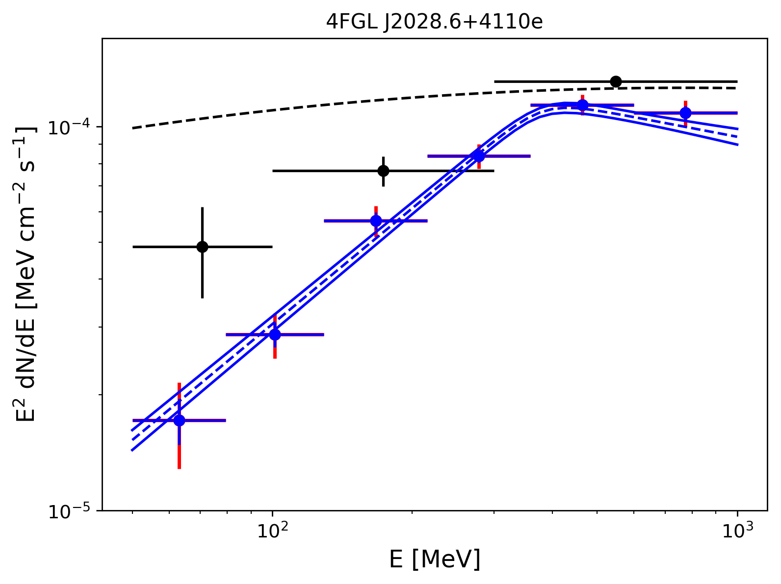
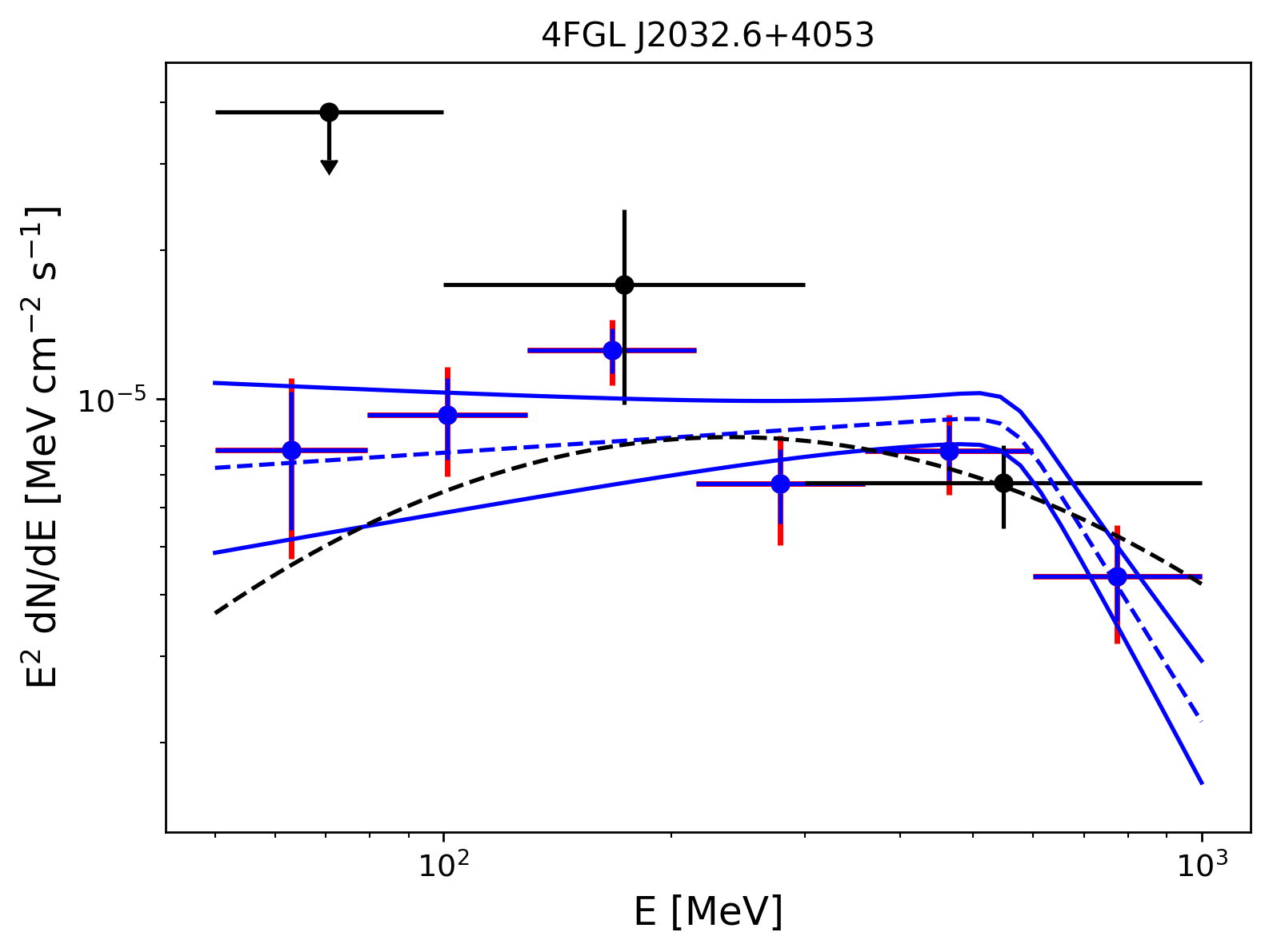
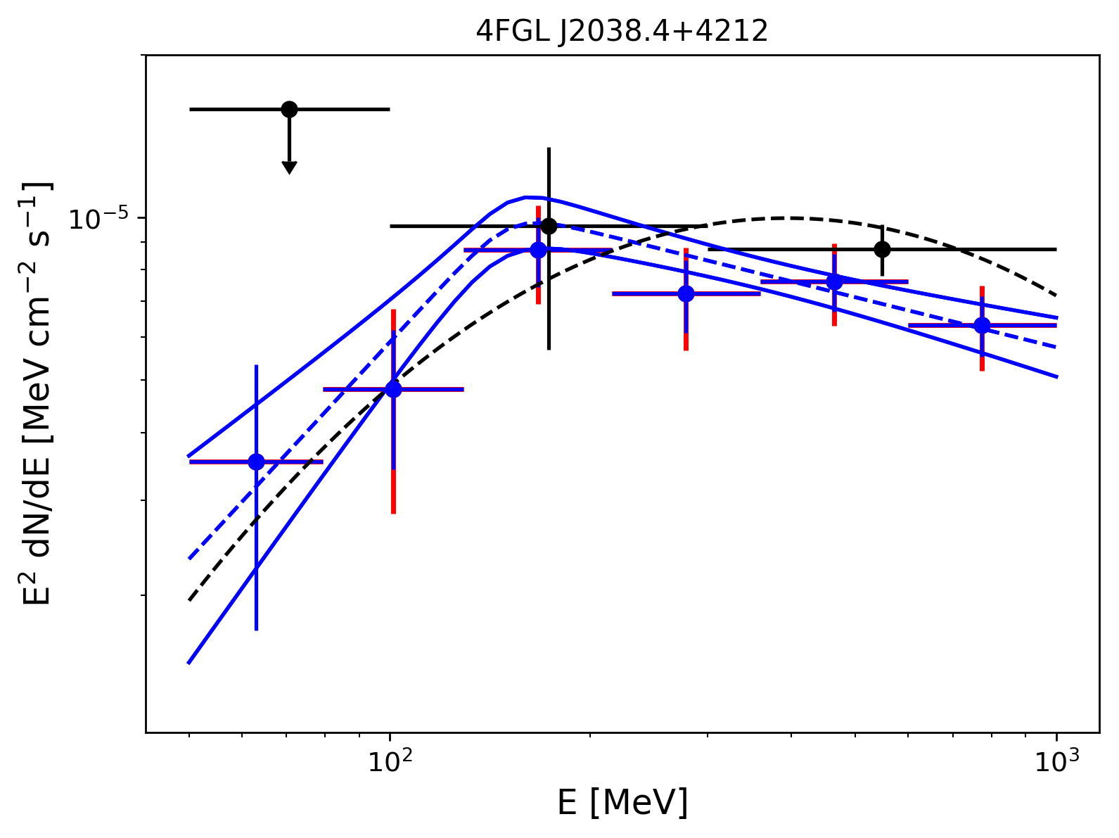
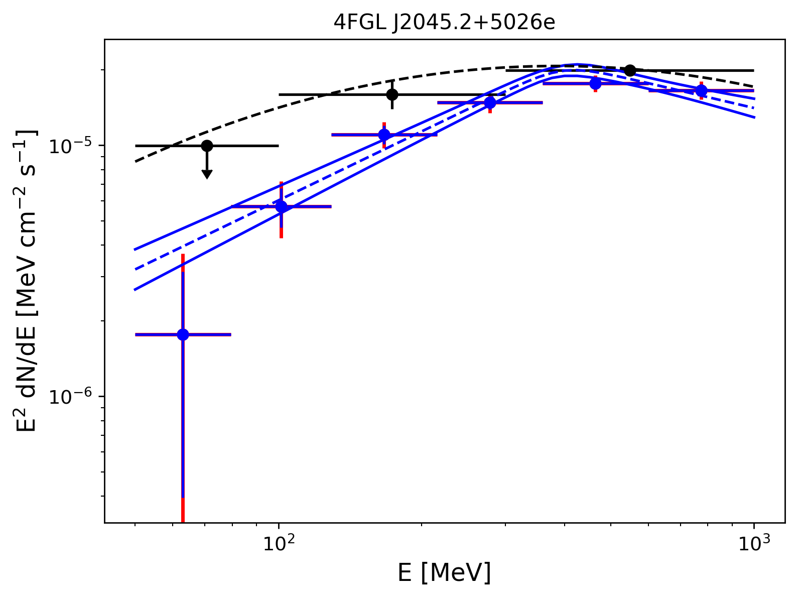
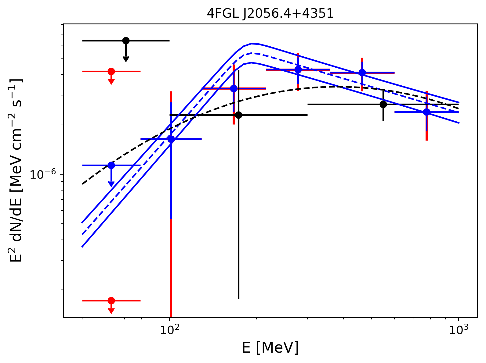
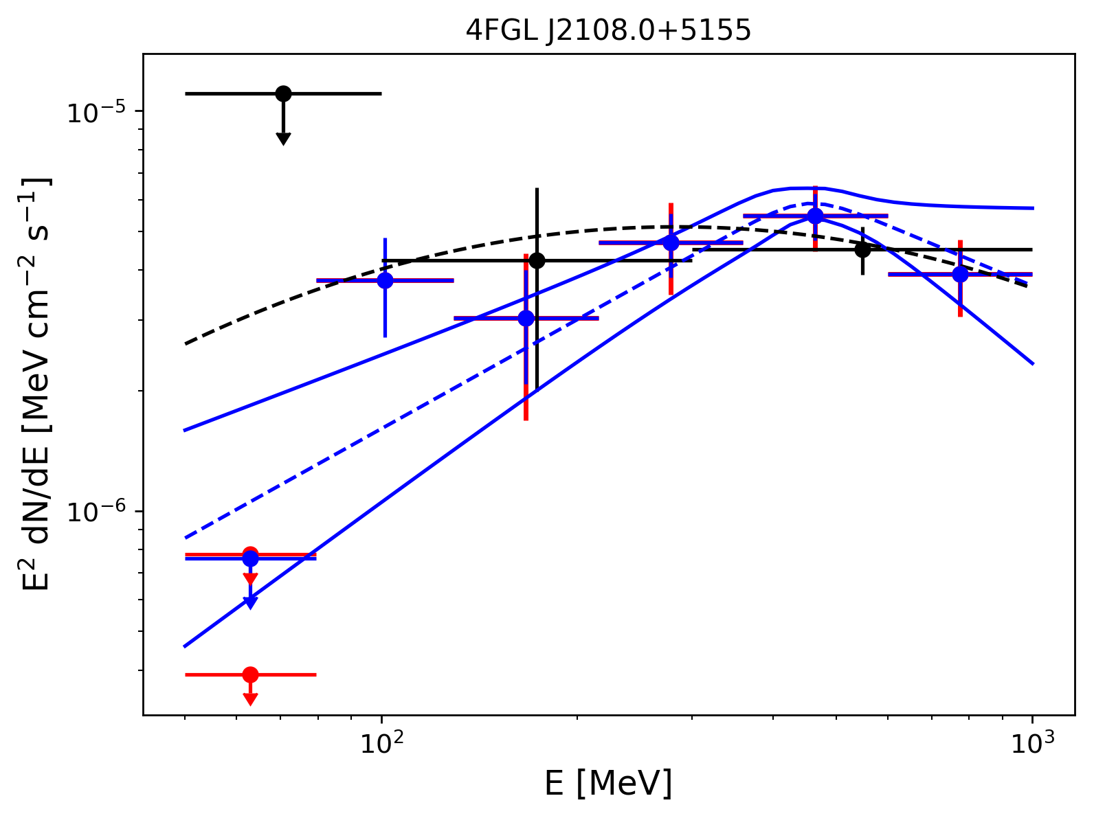
Figure 18: LAT Spectral energy distributions of 4FGL J2028.6+4110e (top left), 4FGL J2032.6+4053 (top right), 4FGL J2038.4+4212 (middle left), 4FGL J2045.2+5026e (middle right), 4FGL J2056.4+4351 (bottom left), 4FGL J2108.0+5155 (bottom right) with the same conventions used in Figure 9.

The most famous sources with “pion bump” signature are the middle-aged remnants IC 443 and W44. Figure 9 presents the residual TS maps of the region of IC 443 (4FGL J0617.2+2234e) and W44 (4FGL J1855.9+0121e) as well as their spectral energy distributions, showing the overall agreement with the 4FGL SED points superimposed. This Figure also illustrates the advantages of using a restricted energy range and different spectral shape than the 4FGL to better reproduce the significant energy break at low energy since we are not dominated here by photons at high energies. The spectral parameters reported in Table 4 for these two sources are in reasonable agreement with those published by Ackermann et al. (2013), knowing that this first analysis did not take into account the effect of energy dispersion and no systematic uncertainties were evaluated at that time.
Among the 56 sources with significant breaks, one can see from the 4FGL Classification column listed in Table 8 that ten sources are firm SNR identifications and three are associated with SNRs. Among the three SNR associations, 4FGL J1911.0+0905 (Figure 17 top right) is associated to W49B and thus can be safely identified as a SNR since it is one of the few other sources for which a “pion decay bump” signature was published with W51C (4FGL J1923.2+1408e, Figure 17 middle left) and HB 21 (4FGL J2045.2+5026e, Figure 18 middle right). The only missing source for which a low-energy break has been published is Cassiopeia A (4FGL J2323.4+5849) but the break energy reported by Yuan et al. (2013) is at $1.72^{+1.35}_{-0.89}$ GeV which seems consistent with our non-detection in the 50 MeV – 1 GeV energy interval. The five sources confirmed by our analysis are all supernova remnants interacting with molecular clouds (MCs). These molecular clouds are excellent targets for cosmic-ray interactions and subsequent pion-decay.
The hadronic scenario was also preferred for other LAT-detected SNRs interacting with MCs, though their $\gamma$-ray analysis starting above a few hundred MeV did not allow rejection of a leptonic scenario: the SNR HB3 and the W3 HII complex (Katagiri et al., 2016b), S147 (Katsuta et al., 2012), HB9 (Araya, 2014), the SNR G326.3$-$1.8 (Devin et al., 2018) and the SNR W28 (Hanabata et al., 2014). Our low-energy analysis presents a rapid turn-over of the spectrum at low energy which confirms the conclusions of the previous publications for 4FGL J0222.4+6156e (W3, see Figure 10 top left), 4FGL J0500.3+4639e (HB9, see Figure 10 bottom right), 4FGL J0540.3+2756e (S147, Figure 11 top left) 4FGL J1552.9$-$5607e (G326.3$-$1.8, Figure 14 middle left) and 4FGL J1801.3-2326e (W28, see Figure 15 middle left). No significant curvature is detected for the SNR HB3 but it should be noted that its $\gamma$-ray emission is much fainter than the adjacent molecular cloud W3 (TS value of 75.9 with respect to 1307.1 for W3) and more data would be needed to constrain the low-energy spectrum of the SNR. A hadronic scenario was also invoked for the SNR Monoceros Loop (Katagiri et al., 2016a). In this case, the brightest gamma-ray peak is spatially correlated with the Rosette Nebula, a young stellar cluster and molecular cloud complex located at the edge of the southern shell of the SNR which has a role similar to W3 for the HB3/W3 complex. The interaction between the SNR and the molecular cloud provides the target to naturally produce gamma rays via proton-proton interaction and it is not a surprise that we confirm a spectral break at low energy for the Monoceros SNR (4FGL J0639.4+0655e, see Figure 11 bottom left) and for the Rosette complex (4FGL J0634.2+0436e, see Figure 11 middle right). More recently, modeling of the non-thermal emission of the gamma Cygni SNR (Fraija & Araya, 2016; Fleischhack, 2019), associated with the source 4FGL J2021.0+4031e, also suggested that the $\gamma$-ray emission (analyzed above 100 MeV) might be of hadronic nature with enhanced GeV emission spatially coincident with the TeV source VER J2019+407. Here again, our low energy analysis detects a low-energy break in the spectrum of this SNR (see Figure 17 bottom right) but it should be noted that the bright $\gamma$-ray emission from the pulsar PSR J2021+4026, lying near the center of the remnant, is very difficult to disentangle from the signal of the SNR at these low energies which could lead to some contamination in the SNR spectrum. A follow-up study in the off-pulse of the pulsar would therefore be needed to confirm the results obtained with our pipeline. This applies not only to supernova remnants but also to all sources coincident with (or very close to) a bright gamma-ray pulsar. It is even more clear for 4FGL J1514.2$-$5909e associated with the pulsar wind nebula MSH 15$-$52 and coincident with the soft gamma-ray pulsar PSR B1509$-$58. The very high low-energy flux visible in Figure 13 (bottom right) is most likely to the associated pulsar PSR B1509$-$58 which is not included in the 4FGL Catalog and would be hard to disentangle from the PWN at these energies.

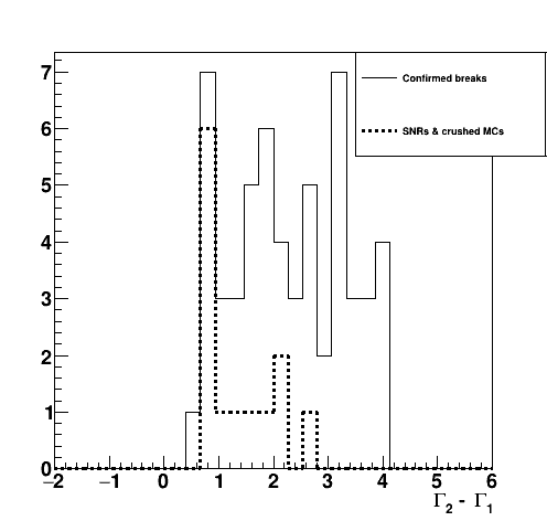
Figure 8: $\Gamma_{1}$ (blue line, left), $\Gamma_{2}$ (red line, left) and $\Gamma_{2}-\Gamma_{1}$ (right) distributions for the 56 sources confirmed by our studies of systematics. In all cases, the dotted line corresponds to the same distribution presented with the solid line but restricted to SNRs (see Section 4.2). The green line indicates the value of $\Gamma_{1}$ obtained using simulations based on the $naima$ package for a proton injection index of 2.0 and the two green dotted-dashed lines indicate the one sigma confidence interval derived (more details in the Appendix A).

4.3 Constraints on other identified sources

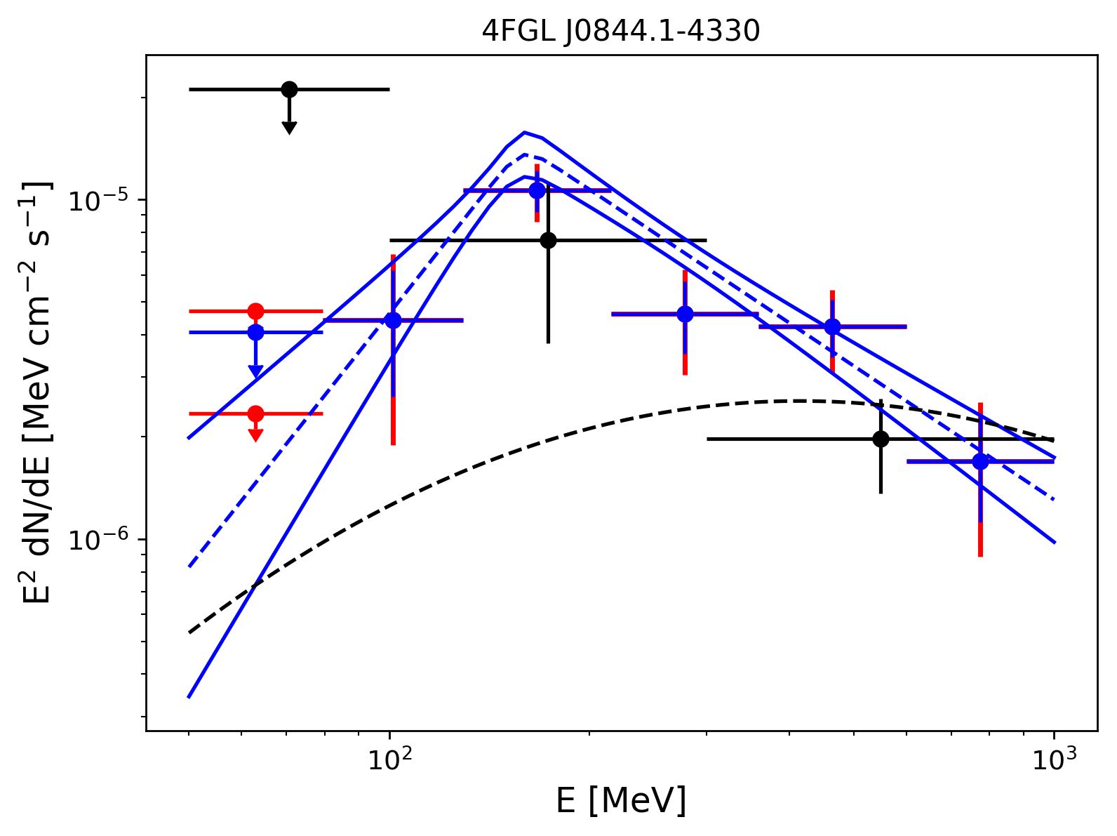
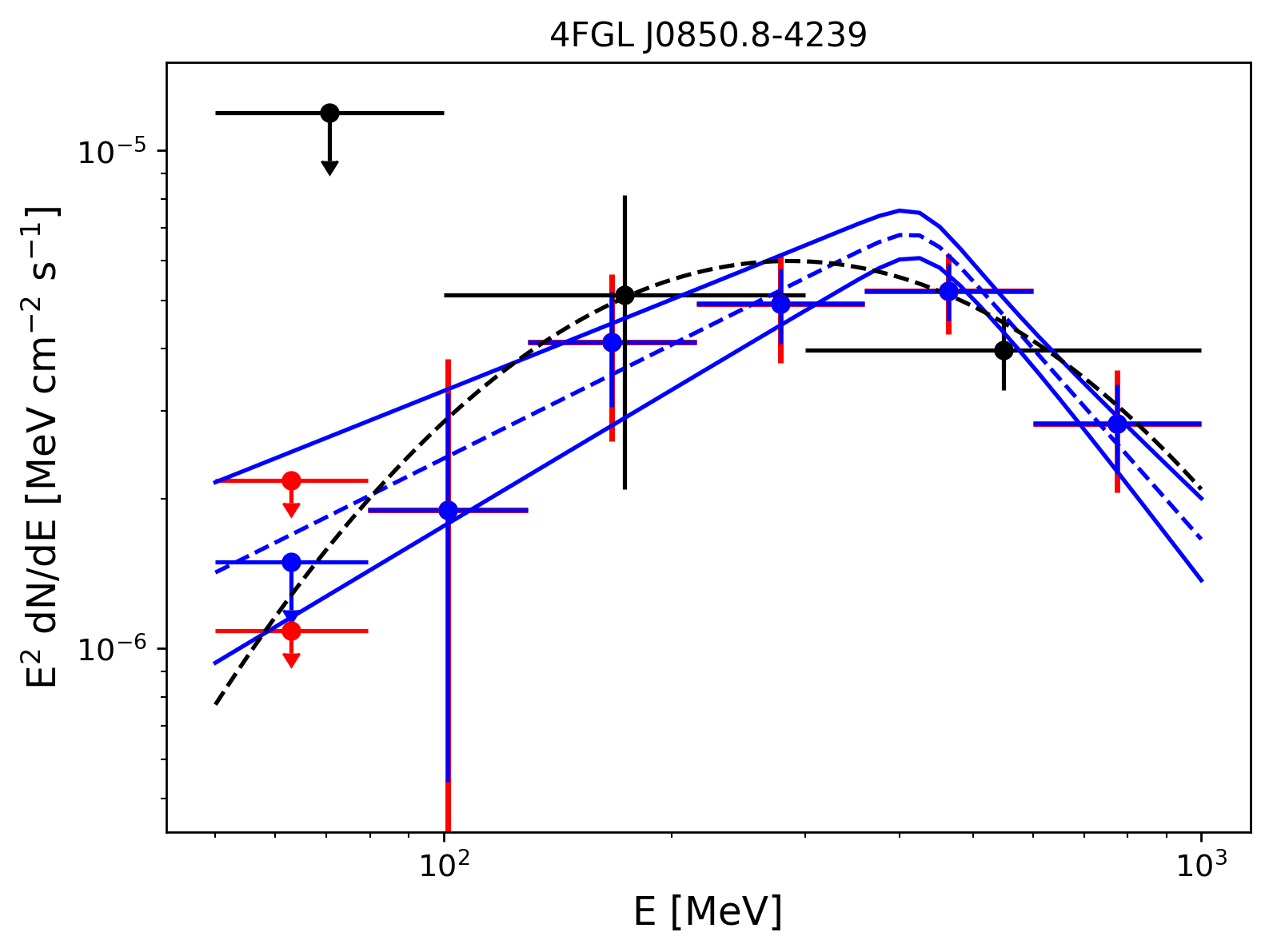
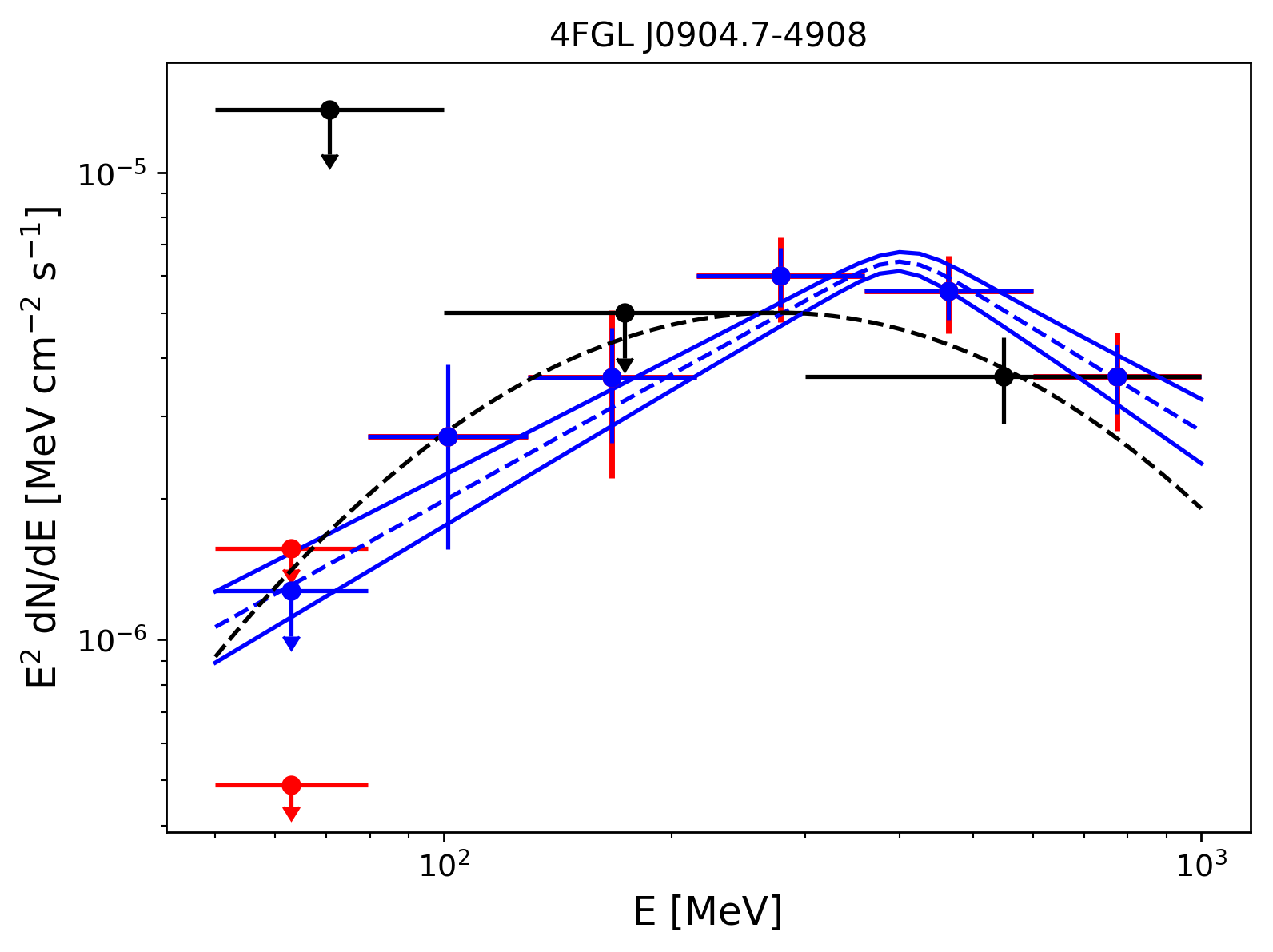
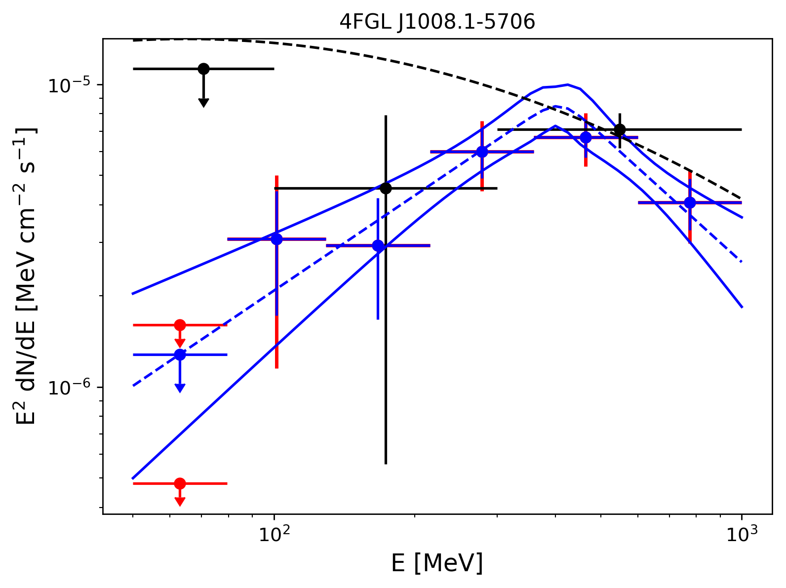
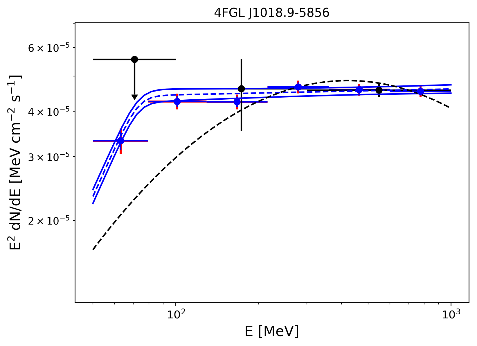
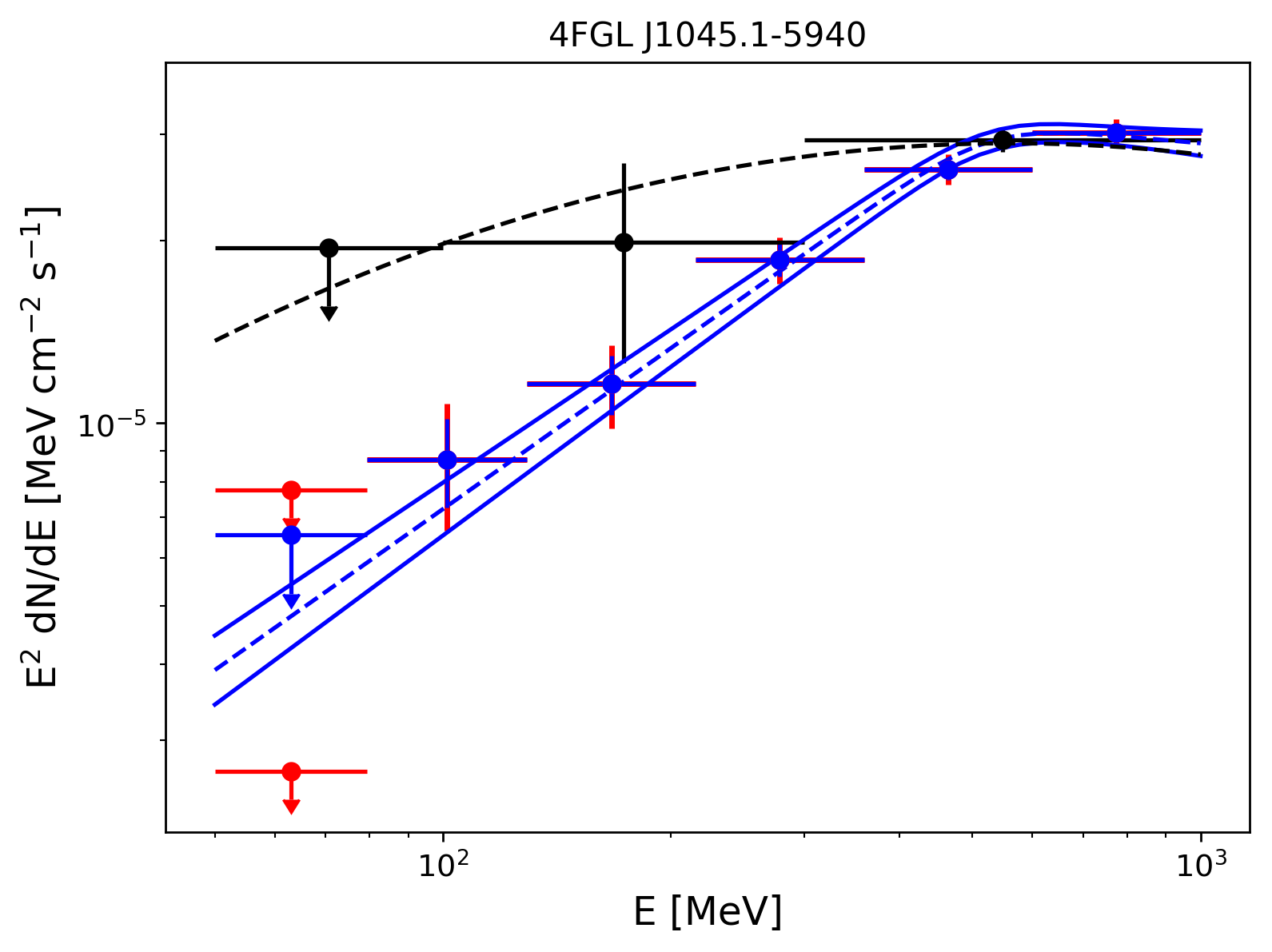
Figure 12: LAT Spectral energy distributions of 4FGL J0844.1$-$4330 (top left), 4FGL J0850.8$-$4239 (top right), 4FGL J0904.7$-$4908 (middle left), 4FGL J1008.1$-$5706 (middle right), 4FGL J1018.9$-$5856 (bottom left), 4FGL J1045.1$-$5940 (bottom right) with the same conventions used in Figure 9.

As discussed in Section 4.2, gamma-ray observations are suggestive of hadron acceleration in a number of SNRs: the young SNRs Tycho and Cassiopeia A, and the middle-aged remnants with “pion decay signature” cited above. However, definite proof of proton acceleration, especially at PeV energies, is still missing and alternative Galactic sources of cosmic rays could play a significant role.
The shocks generated by the stellar winds of massive stars or star-forming regions are among these cosmic-ray accelerators. In this respect, the detection in gamma rays of the Cygnus region by the LAT (Ackermann et al., 2011) opened new perspectives by revealing the presence of a cocoon of freshly-accelerated CRs over a scale of $\sim 50$ pc. Our analysis revealed a spectral break for the star-forming region analyzed, 4FGL J2028.6+4110e (see Figure 18 top left), which is associated with the cocoon. A very hard index $\Gamma_{1}=1.00\pm 0.02_{\rm stat}\pm 0.37_{\rm syst}$ is detected up to a break energy at $383\pm 13_{\rm stat}\pm 138_{\rm syst}$ MeV, followed by a spectral index $\Gamma_{2}=2.23\pm 0.06_{\rm stat}\pm 0.24_{\rm syst}$, similar to those observed for the population of identified SNRs as can be seen in Figure 8. A complete modeling of the source at gamma-ray energies is beyond the scope of this paper but our results tend to favour the hadronic scenario, thus reinforcing the long-standing hypothesis that massive-star-forming regions house particle accelerators.
Gamma-ray binaries, microquasars and colliding wind binaries could also contribute to the sea of Galactic cosmic rays and, at least contribute significantly to the population of sources with significant breaks as reported in Section 4.1. Spectral breaks have been detected for these three types of sources with 4FGL J0240.5+6113 associated with the high-mass $\gamma$-ray binary (HMB) LS I +61 303 (Figure 10 top right), the HMB 4FGL J1018.9$-$5856 (Figure 12 bottom left), 4FGL J1045.1-5940 associated with the colliding wind binary $\eta$ Carinae (Figure 12 bottom right) and 4FGL J2032.6+4053 associated with the microquasar Cyg X-3 (Figure 18 top right). However, this last source presents the highest value of spectral index $\Gamma_{1}$ ($1.90\pm 0.16_{\rm stat}\pm 0.07_{\rm syst}$) among the 56 candidates, which does not really look like the standard “pion bump” signature observed for interacting SNRs. Finally, the source 4FGL J1405.1$-$6119 was recently identified as a high-mass gamma-ray binary using Fermi-LAT observations (Corbet et al., 2019), and should therefore be added to the small set of gamma-ray binaries detected in our analysis. Since significant variability was detected by the LAT for these five $\gamma$-ray sources, an individual analysis taking into account their orbital period would be needed to see if the spectral break detected is a signature of proton-proton acceleration.

4.4 Interesting new cases: potential proton accelerators ?

Among the sources for which a significant spectral break is detected with our pipeline, several are classified as spp, unk or even unassociated as can be seen in Table 5. Among these three source classes, spp is the only one for which the fraction of sources with significant break is similar to the analyzed fraction (11.9% vs 10.7%), while unk and UNIDs both show a clear decrease between the analyzed fraction and the confirmed one (see Figure 5). The spp are sources of unknown nature but overlapping with known SNRs or PWNe and thus candidates to these classes, while unk are sources associated to counterparts of unknown nature. Unassociated, spp and unk represent $29.7$% of the 4FGL sources: revealing the mystery of the nature of these unidentified gamma-ray sources might shed new light on the problem of the origin of galactic CRs. In this respect, three sources detected by our pipeline are of special interest since they are coincident with SNRs and/or dense molecular clouds.
This is the case for 4FGL J1601.3$-$5224 (Figure 14 middle right) coincident with the SNR G329.7+00.4 which presents a diffuse shell at radio energies (Whiteoak & Green, 1996) but is not detected at any other wavelength. Our analysis indicates a soft spectrum $\Gamma_{2}=3.78\pm 0.32_{\rm stat}\pm 0.89_{\rm syst}$ with large systematics due to the diffuse background. The same systematics affect the value of the energy break showing that our results may suffer from contamination.
Similarly, the source 4FGL J1934.3+1859 (Figure 17 bottom left) is coincident with SNR G054.4$-$00.3 detected as a nearly circular shape and angular diameter of $\sim 40$ arcmin at radio energies (Junkes et al., 1992) while Swift and Suzaku X-ray observations allowed the detection of the X-ray counterpart (Karpova et al., 2017) of the gamma-ray pulsar PSR J1932+1916 (Pletsch et al., 2013) located near the edge of the supernova remnant. Suzaku observations also revealed diffuse emission with extent of about 5 arcmin whose spectral properties are compatible with those of PSR+PWN systems. Interestingly, large-scale CO structures across the SNR were observed, indicating the SNR interaction with the ambient molecular gas which is an important ingredient to enhance the gamma-ray emission due to proton-proton interaction. Our analysis reveals a spectral index above the break energy $\Gamma_{2}=3.13\pm 0.27_{\rm stat}\pm 0.12_{\rm syst}$ which may again indicate that the association with an SNR is spurious or that our low-energy analysis suffers from contamination from other neighboring sources in this crowded region.
Finally, the unidentified source 4FGL J1931.1+1656 (Figure 17 middle right) is coincident with the SNR candidate G52.37$-$0.70 detected in a recent THOR+VGPS analysis (Anderson et al., 2017). However, the spectral index of $\alpha=0.3\pm 0.3$ using VLA observations (Driessen et al., 2018) seems to indicate that this candidate is unlikely to be an SNR. The $\gamma$-ray spectrum derived by our analysis resembles that of other SNRs and is not affected by large systematics especially the break energy $203\pm 8\pm 19$ and the spectral index above the break $\Gamma_{2}=2.64\pm 0.10\pm 0.04$. It is the best candidate for proton acceleration among these three potential SNR association.
These three regions are extremely complex and would deserve a dedicated analysis at higher energy with Fermi to constrain their location and their association with the corresponding SNR, as well as a spectral analysis over a larger energy interval to definitively constrain the type of radiating particles.
Even more care should be taken for the extended sources 4FGL J1633.0$-$4746e (Figure 15 top left) and 4FGL J1813.1$-$1737e (Figure 15 bottom right) since their disk radii of $0.61^{\circ}$ and $0.6^{\circ}$ respectively in confused Galactic plane regions adds to the complexity of such analysis at low energy. With its large extension, 4FGL J1633.0$-$4746e overlaps with both the TeV PWN candidate HESS J1632$-$478 and the unidentified source HESS J1634$-$472, both detected at GeV energies but not included in our list of selected candidates due to their low significance at low energy. This implies that the region contains three sources: a point-like source coincident with HESS J1634$-$472, an extended source coincident with HESS J1632$-$478 but with an extension of $0.256^{\circ}$ almost twice as large as the TeV size, and the very extended source 4FGL J1633.0$-$4746e overlapping them detected above 10 GeV with a spectral index of $2.25\pm 0.01_{\rm stat}\pm 0.10_{\rm syst}$ (Ackermann et al., 2017). Interestingly, our spectral analysis indicates a break at $517\pm 18_{\rm stat}\pm 252_{\rm syst}$ MeV followed by an index of $\Gamma_{2}=2.11\pm 0.15_{\rm stat}\pm 0.12_{\rm syst}$ in agreement with the index detected above 10 GeV (though with very large systematics on the break energy due to the diffuse background). The break detected at low energy by our analysis, the hard spectral index $\Gamma_{2}$ consistent with the one detected at higher energy (which seems to indicate a flat spectrum over a large energy range) and the presence of dense clumps in this region traced NH₃(1,1) emission (de Wilt et al., 2017) make this source a very interesting proton accelerator. A dedicated analysis would therefore be very valuable in this case.
The disk radius of $0.60\pm 0.06_{\rm stat}^{\circ}$ of the Fermi source 4FGL J1813.1$-$1737e, coincident with the compact TeV PWN candidate HESS J1813$-$178 (Gaussian size of $0.049\pm 0.04^{\circ}$ in H. E. S. S. Collaboration et al., 2018b), was first detected by Araya (2018). The authors reported a hard index of $2.07\pm 0.09_{\rm stat}$ above 500 MeV compatible with the TeV index. This spectrum is compatible with the spectral index $\Gamma_{2}=2.17\pm 0.03_{\rm stat}\pm 0.42_{\rm syst}$ derived in our analysis. With such a large extension in the Galactic plane, several sources could contribute to the GeV signal: the PWN powered by PSR J1813$-$1749 thought to emit at TeV energies as seen by H.E.S.S. and HAWC (Abeysekara et al., 2017), the SNR G12.82$-$0.02 whose contribution to the TeV signal was explored by Funk et al. (2007) and the giant star-forming region (SFR) W33 that comprises a region of 15’ at a distance of 2.4 kpc (Immer et al., 2013). This last hypothesis was considered by Araya (2018), showing that the energetics, extended morphology and spectrum of the GeV emission are similar to those of the other gamma-ray detected SFR, the Cygnus Cocoon. To firmly establish the presence of protons radiating at gamma-ray energies, such a complex region definitively is worth an individual analysis above 1 GeV to constrain the morphology and a spectral analysis over a larger energy range to model the broad-band emission.
Finally, several sources detected by our analysis are completely unassociated and follow-up observations at TeV energies and X-rays would be needed to constrain their nature. They all present values of $\Gamma_{2}$ much softer than those of the identified SNRs discussed in Section 4.2. Similarly, the values of $\Gamma_{2}-\Gamma_{1}$ obtained in our analysis is much larger ($\geq 2.96$) than those of the identified SNRs and dense molecular cloud regions. This tends to indicate that these sources are not associated with SNR shock acceleration.

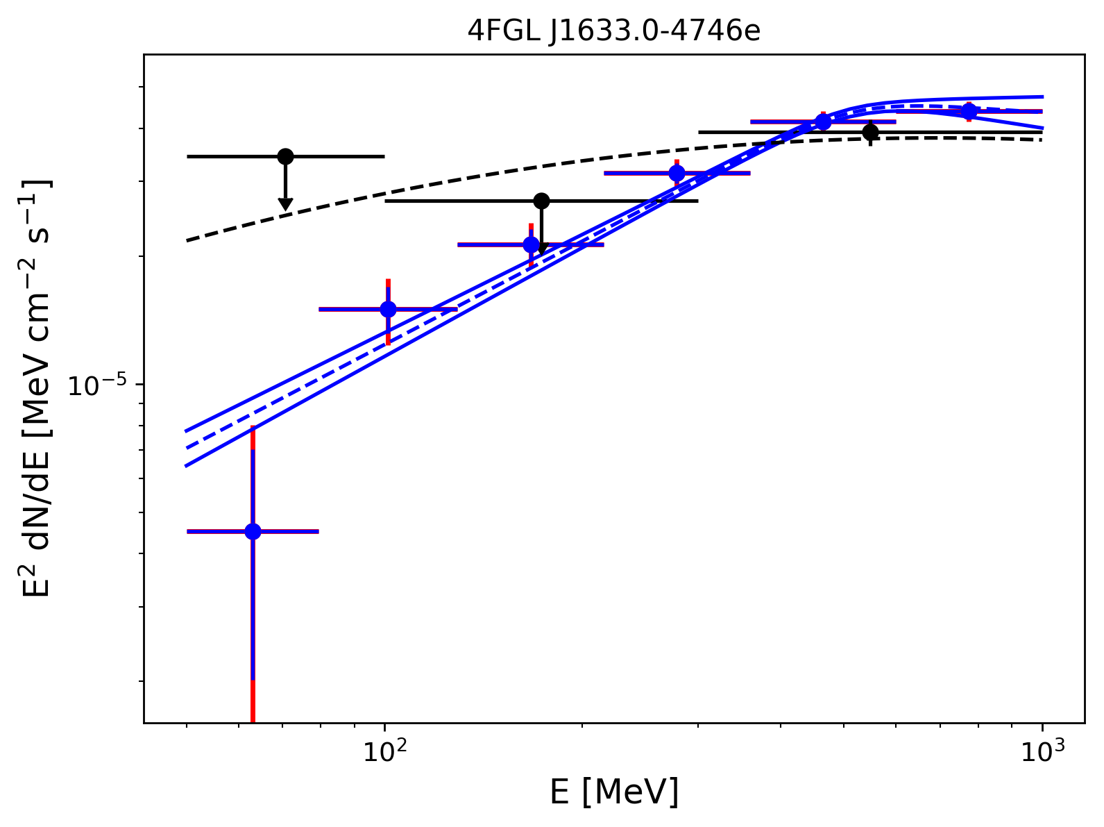
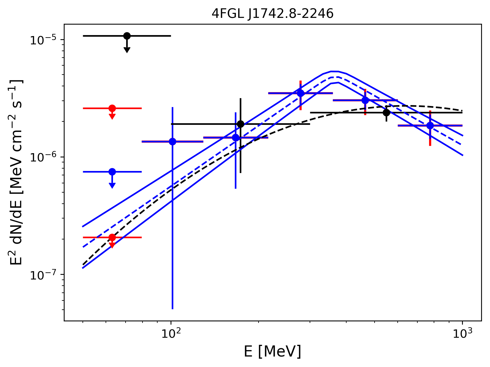
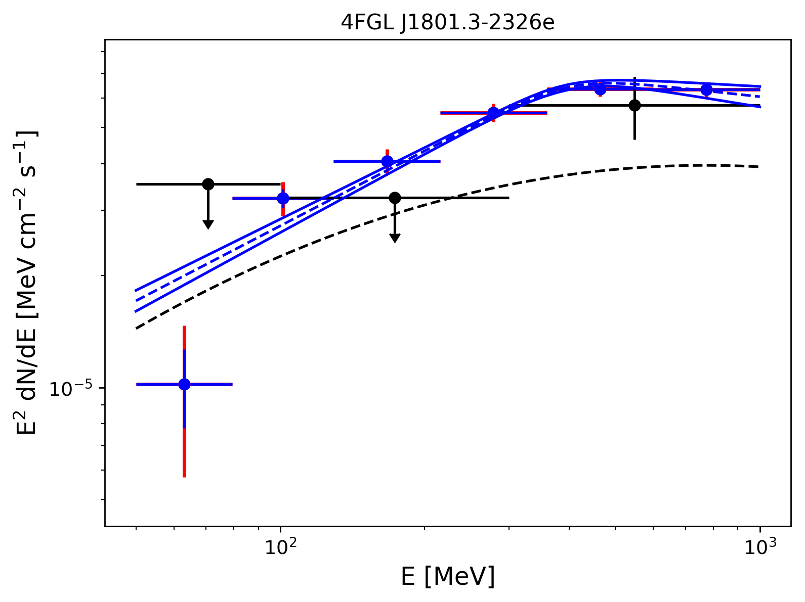
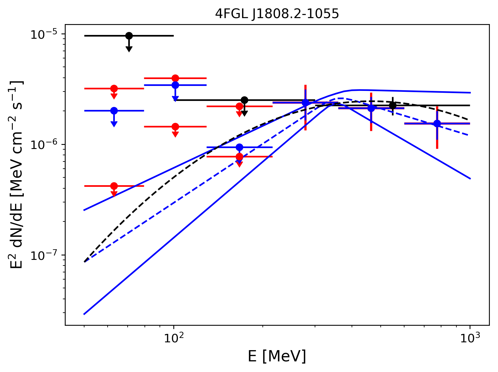
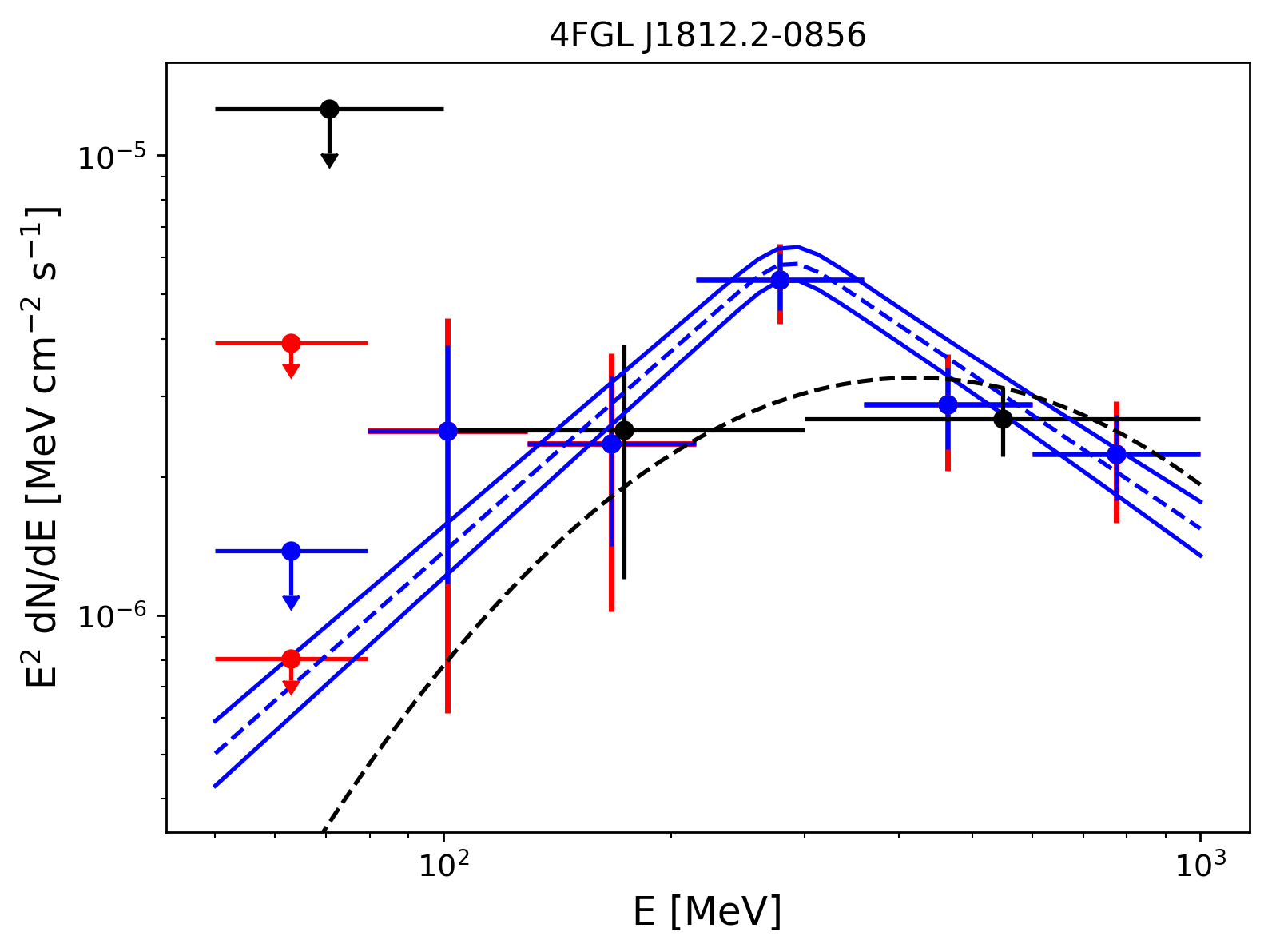
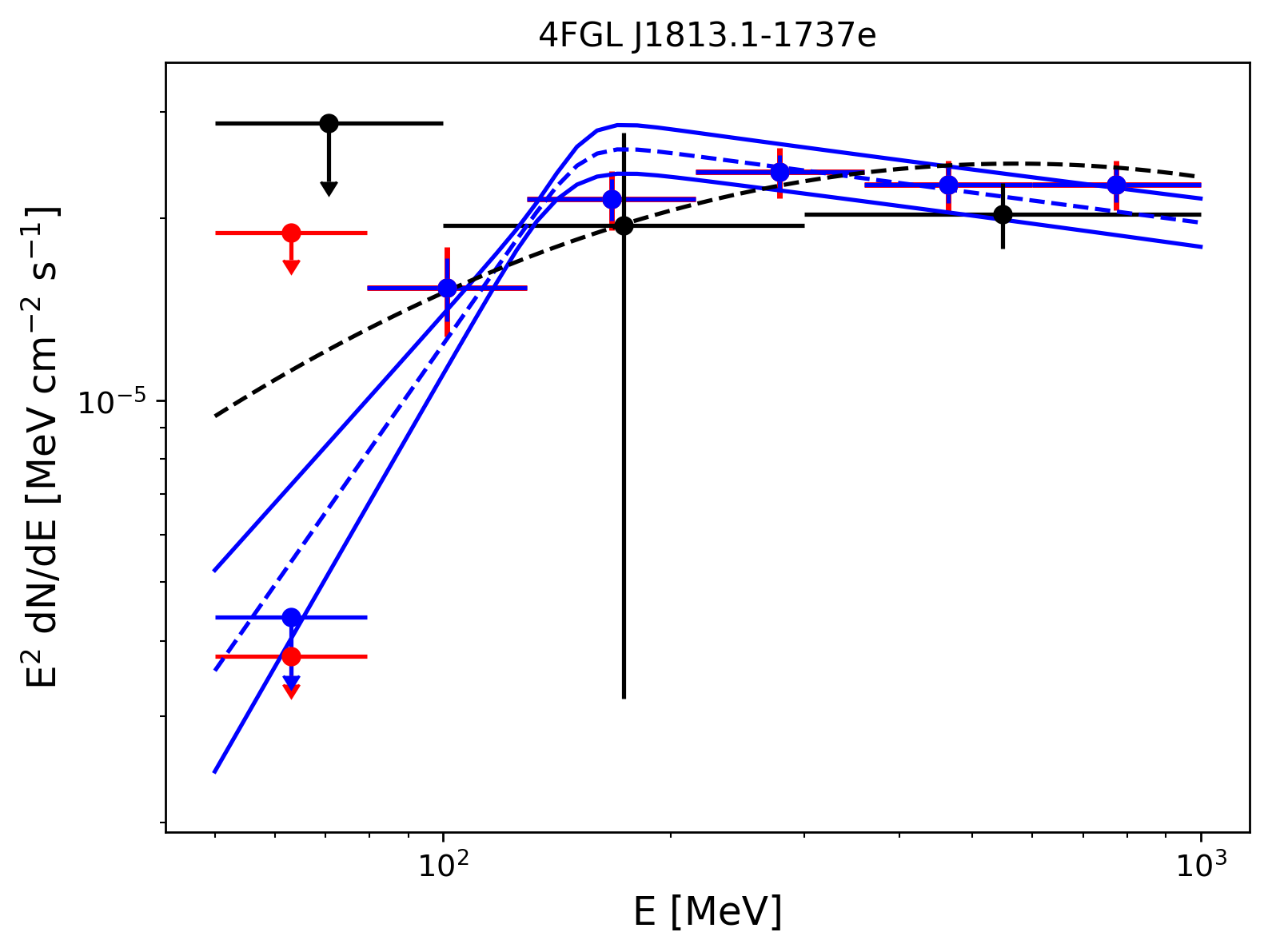
Figure 15: LAT Spectral energy distributions of 4FGL J1633.0$-$4746 (top left), 4FGL J1742.8$-$2246 (top right), 4FGL J1801.3$-$2326e (middle left), 4FGL J1808.2$-$1055 (middle right), 4FGL J1812.2$-$0856 (bottom left), 4FGL J1813.1$-$1737e (bottom right) with the same conventions used in Figure 9.

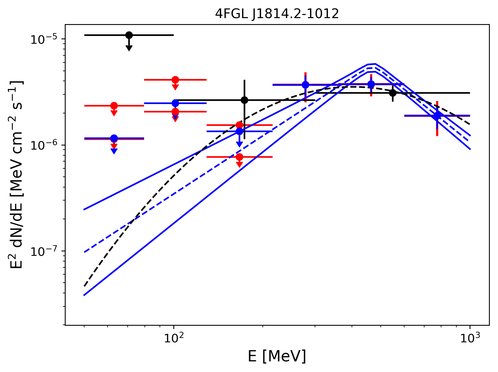
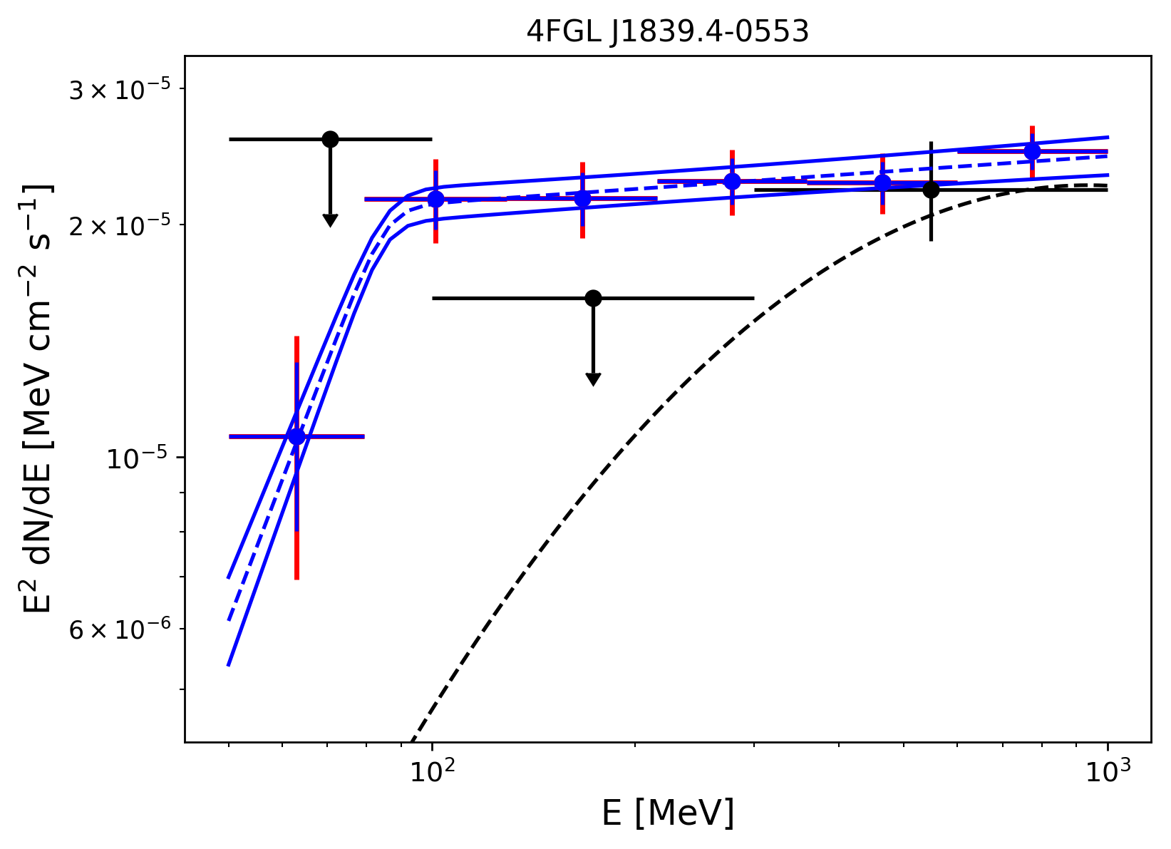
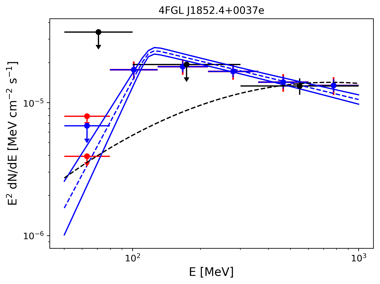
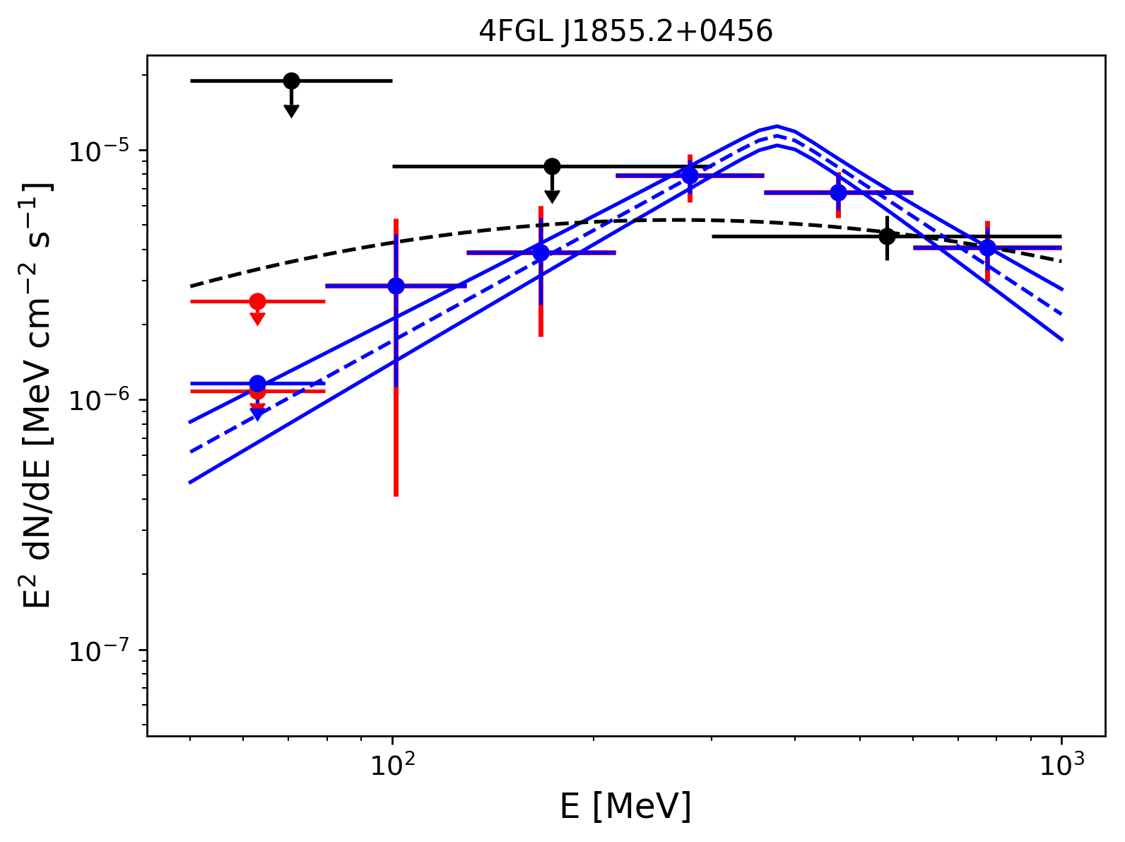
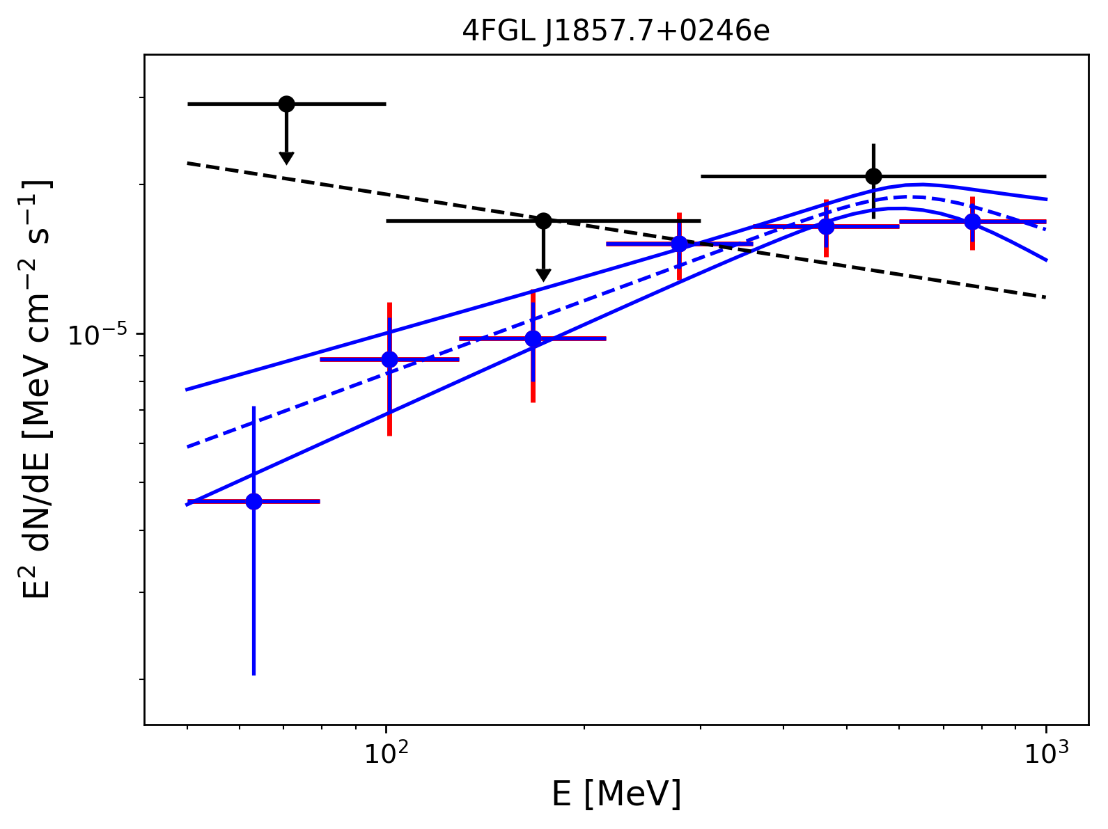
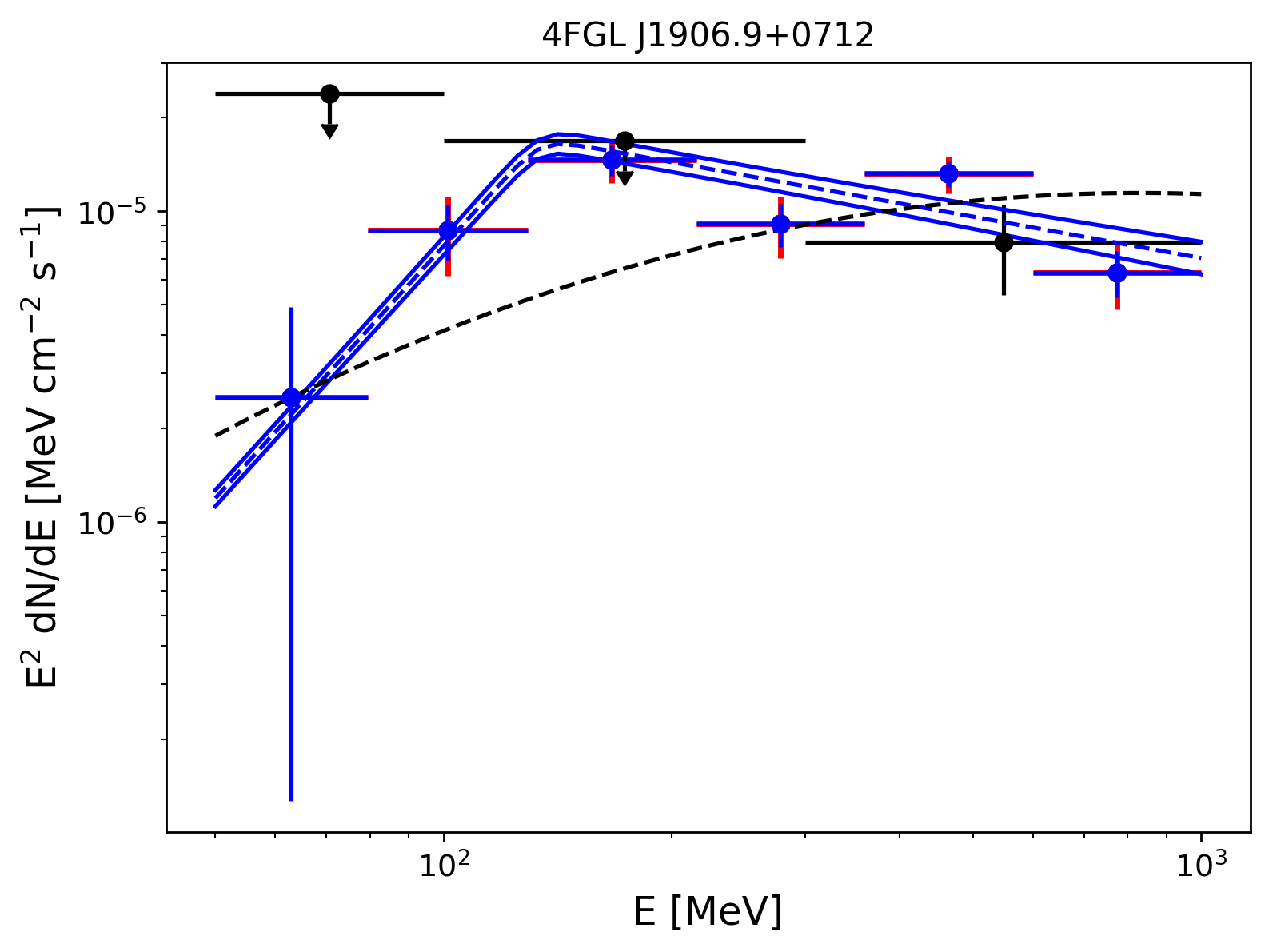
Figure 16: LAT Spectral energy distributions of 4FGL J1814.2$-$1012 (top left), 4FGL J1839.4$-$0553 (top right), 4FGL J1852.4+0037e (middle left), 4FGL J1855.2+0456 (middle right), 4FGL J1857.7+0246e (bottom left), 4FGL J1906.9+0712 (bottom right) with the same conventions used in Figure 9.

5 Summary

Using 8 years of Pass 8 LAT data between 50 MeV and 1 GeV, we have analyzed 311 4FGL sources located within $5^{\circ}$ from the Galactic plane and detected 77 sources with significant spectral breaks. We carried out a thorough study of the systematics associated with the diffuse Galactic background and with the effective area for each of them and we confirmed the spectral break for 56 of them. With 13 SNRs identified within this sample of 56 sources, SNRs are the dominant class of sources showing significant breaks at low energy. Only five binaries are included in the sample of 311 sources analyzed but four of them show a significant break at low energies. This seems to indicate that binaries could also have a significant contribution. The spectral characteristics were also evaluated for these 56 sources. The break energy of the sources ranges uniformly between 100 MeV and 550 MeV. However, a clear pattern is detected in the spectral index $\Gamma_{2}$ of the sources which tends to center at $2.3$ for the population of 13 identified SNRs. Similarly, the value of $\Gamma_{2}-\Gamma_{1}$ tends to center at $\sim 1$ for the same population of sources. This provides an interesting way to constrain the nature of the radiating particles. Our analysis also provides three interesting new proton accelerator candidates: 4FGL J1931.1+1656 is coincident with the SNR candidate G52.37$-$0.70 detected in a recent THOR+VGPS analysis, the extended source 4FGL J1633.0$-$4746e overlapping the TeV PWN candidate HESS J1632$-$478 and the unidentified source HESS J1634$-$472, and the extended source 4FGL J1813.1$-$1737e coincident with the compact TeV PWN candidate HESS J1813$-$178 and the star-forming region W33. The current and future observations of the LAT are thus crucial to probe the spectral characteristics of a source at low energy, providing excellent targets of proton acceleration for current and future Cherenkov telescopes such as CTA.

Appendix A The pion-decay bump signature

As already discussed in the main text, when accelerated protons interact with the interstellar matter, they produce neutral pions which in turn decay into gamma rays. This will create a characteristic signature at low energy in the gamma-ray spectrum called the “pion-decay bump signature”. To better understand how this signature is characterized in our energy interval of interest (50 MeV – 1 GeV), we have used the python package $naima$ (Zabalza, 2015) to derive the gamma-ray emission produced by proton-proton interaction. To do so, $naima$ uses an implementation of the analytical parametrizations of the energy spectra and production rates of gamma rays from Kafexhiu et al. (2014), which is accurate within $20$%. The inclusive $\pi^{0}$ production cross section is included as a combination of the experimental data cross sections at low energies, the Geant 4.10.0 cross section at intermediate energies and at higher energies the hadronic model Pythia 8.18 as default. We applied $naima$ to three different power-law distributions of protons with spectral index $\Gamma_{1}$ varying between 1.5 and 2.5. The results presented in Figure 19 (Left) are in perfect agreement with those published in Ackermann et al. (2013) and show that a very steep spectrum is expected below the break energy at $\sim 200$ MeV. This Figure also highlights that the pion-decay bump signature might be more difficult to detect for a hard proton distribution (red curve) than for steep injection spectra. This might in turn increase the systematic errors on the derived break energy. Finally, this Figure demonstrates that the restricted energy interval of our analysis does not allow constraining the spectral index of the parent distribution since the gamma-ray spectra trace the energy distribution of parent protons at energies greater than 1 GeV. The upper bound of our energy interval was chosen since middle-aged SNRs commonly exhibit a high energy spectral break at around 1–10 GeV (see the case of W28 with a break at 1 GeV reported by Abdo et al., 2010) and a simple broken power-law model would not apply anymore above 1 GeV. To test for this effect, we applied $naima$ to the same power-law distributions of protons adding a break at 1 GeV in their distributions. We assumed that $\Gamma_{2}=\Gamma_{1}+1$. Figure 19 (Right) demonstrates that the break energy of the gamma-ray emission detected in our energy interval is not affected. However, this break significantly impacts the spectral index derived assuming a simple broken power-law model. In a second step, we used the gamma-ray emission obtained with $naima$ assuming a power-law distribution of protons with $\Gamma_{1}=2.0$ and $2.5$ to produce 200 Fermi simulated data files for each index over 8 years using the $gtobssim$ tool included in the LAT $fermitools$. We then analyzed these simulations using the $fermitools$ following the same procedure as with the real data, assuming a smooth broken power-law spectral model with $\alpha=0.1$ (see Equation 1), except that the SED was produced for 12 energy bins instead of 6 to reflect the high statistics of our simulations (which mimics the flux of IC 443). We did not introduce any diffuse background in our simulations to clearly show how a proton spectrum will be reconstructed at low energies with the LAT in the absence of systematic errors. Figure 20 presents the gamma-ray spectrum derived for one of these simulations demonstrating that the spectral index derived above the break does not trace the parent proton distribution. The error bars are extremely small due to the high flux of the simulated source and the absence of diffuse background. This Figure also shows that the smooth broken power-law model used in our analysis with $\alpha=0.1$ reproduces the gamma-ray spectrum well. A smoothness parameter $\alpha=0.5$ was also tested but it does not significantly improves the likelihood of the fit. Finally, one can see that the injection spectral index does not seem to impact the break energy and the index $\Gamma_{1}$ of our smooth broken power-law fit. The only parameter affected is the index $\Gamma_{2}$. To confirm this trend, we plotted the distributions of the 200 reconstructed values of the break energy, $\Gamma_{1}$ and $\Gamma_{2}$ for each injection spectral index, and fitted a Gaussian on each distribution as can be seen in Figure 20 (Right) for the case of the break energy. The results are presented in Table 7 confirming that the only parameter affected by the different injection spectral index is $\Gamma_{2}$. This study demonstrates that no steep spectrum is predicted for a standard injection spectral index. The only way to produce the steep spectra observed for some of the candidates detected in our analysis would be to include an energy break at (or below) 1 GeV in the injection proton spectrum as shown in Figure 19 (Right).

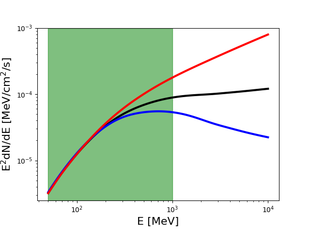
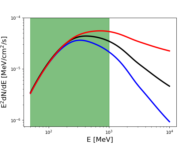
Figure 19: Left: Gamma-ray spectra produced by a power-law distribution of protons with spectral index of 1.5 (red), 2.0 (black), 2.5 (blue) as predicted by $naima$ (Zabalza, 2015). Right: Same figure assuming that an energy break is present in the particle distribution at 1 GeV. The energy interval analyzed in this work is defined by the green area.

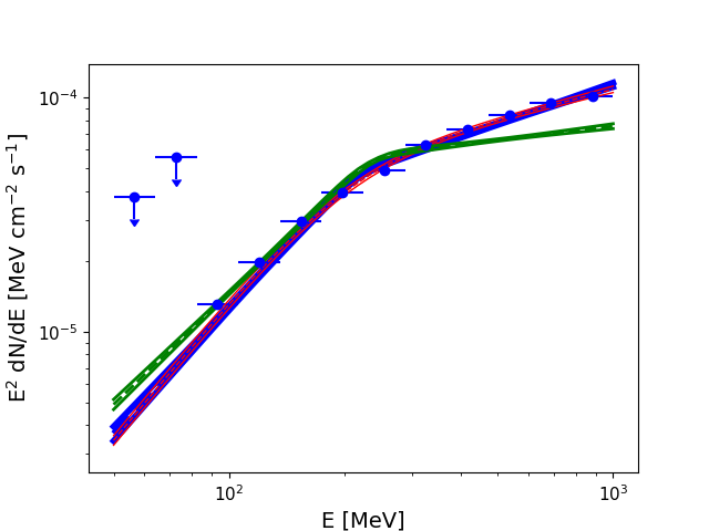
Figure 20: Left: Gamma-ray spectrum derived using our analysis pipeline from one simulation of a power-law distribution of protons with spectral index of 2.0 predicted by $naima$ (Zabalza, 2015). The fit assuming a smooth broken power-law model (see Equation 1) with $\alpha=0.1$ is presented with the blue curve. The fit assuming $\alpha=0.5$ is presented with the red curve. The best fit of a similar simulation assuming a proton injection index of 2.5 is presented with the green line. Right: Distribution of the 200 values of energy break fitted for a proton injection spectral index of 2.0. The black line represents our best Gaussian fit.

Table 7: Results of the Gaussian fits of the 200 $naima$ simulations assuming a proton injection spectral index of 2.0 and 2.5.

	Proton index = 2.0	Proton index = 2.5
Energy break	$209$ / $18$	$212$ / $15$
$\Gamma_{1}$	$0.24$ / $0.09$	$0.29$ / $0.09$
$\Gamma_{2}$	$1.43$ / $0.04$	$1.74$ / $0.04$

Appendix B List of the 311 Galactic plane sources analyzed

Table 8 provides the list of all candidates analyzed. Columns 2 and 3 provide the Galactic longitude and latitude of the 311 candidates. Columns 4, 5 and 6 give the curvature significance, the significance between 300 MeV and 1 GeV and the source class reported in the 4FGL catalog. Columns 7, 8, 9, 10 provide the values obtained in our analysis concerning the TS of each source, the improvement of the log-normal representation with respect to the power-law model ${\rm TS_{LP}}$ as defined in Section 3.2, the improvement of the smooth broken power-law representation with respect to the power-law model ${\rm TS_{SBPL}}$ and the improvement of the smooth broken power-law representation when fixing $\Gamma_{2}=2$ called ${\rm TS_{SBPL2}}$.

Table 8: List of selected Galactic plane candidates

4FGL Name	GLON	GLAT	4FGL SigCurv	4FGL $\sqrt{\rm TS}$	4FGL Class	TS	${\rm TS_{LP}}$	${\rm TS_{SBPL}}$	${\rm TS_{SBPL2}}$
	(∘)	(∘)		(0.3 – 1 GeV)
4FGL J0034.6+6438	121.13	1.83	2.6	3.9		7.6
4FGL J0039.1+6257	121.54	0.12	7.0	5.2		43.8	7.0
4FGL J0129.0+6312	127.16	0.65	3.1	5.7	spp	55.9	5.1
4FGL J0142.5+6650	127.93	4.46	3.4	3.6		6.4
4FGL J0144.3+5959	129.51	$-$2.20	0.6	3.4		4.9
4FGL J0211.5+6219	132.09	0.89	1.1	3.5		0.3
4FGL J0221.4+6241e	133.05	1.60	5.7	8.8	SNR	75.9	0.5
$\star$4FGL J0222.4+6156e	133.42	0.94	14.3	30.7	snr	1307.1	27.2	34.8	32.4
4FGL J0235.3+5650	136.82	$-$3.19	4.1	7.6		77.1	3.7
$\star$4FGL J0240.5+6113	135.68	1.09	28.2	107.3	HMB	39495.7	127.8	127.3	100.9
4FGL J0302.7+5717	139.97	$-$1.17	0.8	3.3		20.3
4FGL J0328.5+6114	140.71	3.92	1.4	3.9		12.3
4FGL J0330.1+5038	146.91	$-$4.70	4.7	6.1		34.8	2.7
$\star$4FGL J0330.7+5845	142.35	2.02	4.7	6.2		43.2	16.1	18.0	14.2
$\star$4FGL J0340.4+5302	146.79	$-$1.82	12.3	23.4		1329.3	149.4	143.6	139.0
$\star$4FGL J0426.5+5434	150.88	3.82	9.8	18.1		704.1	19.6	25.2	18.9
4FGL J0452.9+5117	155.99	4.63	2.8	5.6		26.4	8.0
$\star$4FGL J0500.3+4639e	160.37	2.69	5.8	12.6	SNR	253.0	15.2	19.8	17.1
4FGL J0532.6+3358	174.26	0.36	1.3	3.5		11.2
4FGL J0533.9+2838	178.89	$-$2.33	0.3	3.4	spp	24.7
$\star$4FGL J0540.3+2756e	180.24	$-$1.50	4.5	10.0	SNR	202.0	10.8	12.4	9.2
4FGL J0608.8+2034	189.87	0.35	2.9	3.8	unk	15.2
4FGL J0609.0+2136	188.99	0.89	4.2	3.5		33.3	10.6	9.3	7.5
$\star$4FGL J0609.0+2006	190.31	0.17	4.9	3.9		72.4	12.4	15.1	12.9
4FGL J0612.6+1520	194.89	$-$1.37	3.9	4.4		18.7
$\star$4FGL J0617.2+2234e	189.05	3.03	20.8	17.0	SNR	5456.4	84.5	99.0	79.8
4FGL J0618.7+1211	198.38	$-$1.56	2.9	4.7		65.4	14.6	16.3	15.0
$\star$4FGL J0620.4+1445	196.30	0.00	1.5	3.6		33.5	12.0	16.2	10.4
$\star$4FGL J0634.2+0436e	206.87	$-$1.70	8.4	15.5	snr	370.6	13.1	19.7	19.4
$\star$4FGL J0639.4+0655e	205.40	0.50	7.8	10.2	SNR	170.7	44.6	42.4	39.2
4FGL J0642.4+1048	202.28	2.94	2.7	3.5		12.7
4FGL J0647.7+0031	212.05	$-$0.57	1.1	6.5	spp	48.7	8.5
4FGL J0705.8$-$0004	214.64	3.17	3.1	3.2		15.8
$\star$4FGL J0709.1$-$1034	224.35	$-$0.92	4.3	7.8		80.8	17.0	21.9	14.9
4FGL J0722.7$-$2309	237.01	$-$3.88	3.5	4.4		62.2	17.3	21.5	6.9
4FGL J0731.5$-$1910	234.48	$-$0.19	2.8	5.0		53.8	14.4	18.4	8.0
4FGL J0744.0$-$2525	241.35	$-$0.74	8.0	13.7		200.6	2.4
4FGL J0752.0$-$2931	245.78	$-$1.28	4.0	5.4		36.2	0.6
4FGL J0822.1$-$4253e	260.31	$-$3.37	5.9	16.7	SNR	468.2	3.9
4FGL J0833.3$-$4342	262.17	$-$2.20	0.0	3.7	spp	78.7	8.4
$\star$4FGL J0844.1$-$4330	263.19	$-$0.53	3.2	3.4		65.6	18.2	23.7	12.3
4FGL J0844.9$-$4117	261.55	0.97	3.2	7.0		63.3	6.7
4FGL J0848.8$-$4328	263.69	0.16	1.8	6.8		87.9	6.6
$\star$4FGL J0850.8$-$4239	263.30	0.96	5.0	6.9		83.6	19.5	28.5	19.8
4FGL J0851.9$-$4620e	266.26	$-$1.23	1.1	12.0	SNR	259.8	4.4
4FGL J0853.1$-$4407	264.70	0.35	5.0	5.8		37.8	5.2
4FGL J0853.6$-$4306	263.98	1.07	5.6	7.3		43.8	0.4
4FGL J0854.8$-$4504	265.61	$-$0.03	8.4	5.8		90.6	6.0
4FGL J0857.7$-$4507	265.98	0.33	2.1	5.8		23.8
4FGL J0859.2$-$4729	267.94	$-$1.03	3.9	7.0		135.0	6.9
4FGL J0859.3$-$4342	265.10	1.46	5.9	11.5		105.2	6.8
4FGL J0900.2$-$4608	267.03	$-$0.01	3.1	4.4		43.6	9.7	11.9	6.5
$\star$4FGL J0904.7$-$4908c	269.78	$-$1.44	3.7	5.4	unk	51.8	15.9	16.0	9.5
4FGL J0911.6$-$4738	269.46	0.43	0.9	5.4		72.1	11.2	15.2	8.6
4FGL J0917.9$-$4755	270.39	0.99	4.2	6.2		56.8	3.7
4FGL J0924.1$-$5202	274.01	$-$1.21	1.5	4.9		53.0	22.7	25.5	14.5
$\star$4FGL J1008.1$-$5706c	282.13	$-$0.98	3.3	8.6	unk	118.4	17.8	20.5	19.7
4FGL J1015.5$-$6030	284.87	$-$3.22	2.4	8.8		75.3	5.1
$\star$4FGL J1018.9$-$5856	284.35	$-$1.68	21.2	27.7	HMB	1800.8	10.7	22.9	20.5
4FGL J1020.4$-$5314	281.41	3.20	3.1	4.3		23.0
4FGL J1036.3$-$5833e	286.08	$-$0.18	5.0	8.0		57.9	8.0
4FGL J1037.8$-$5810	286.06	0.24	4.2	6.5		55.0	0.7
$\star$4FGL J1045.1$-$5940	287.60	$-$0.62	12.5	26.4	BIN	1011.6	15.5	18.9	16.7
4FGL J1045.7$-$6414	289.79	$-$4.63	1.9	3.8	unk	10.3
4FGL J1046.7$-$6010	288.01	$-$0.97	6.2	5.8		55.7	2.8
4FGL J1048.5$-$5923	287.85	$-$0.17	7.6	4.7		60.1	3.4
4FGL J1054.7$-$6008	288.88	$-$0.49	1.6	3.5		21.4
4FGL J1102.0$-$6054	290.02	$-$0.81	6.8	7.0	spp	77.2	4.1
4FGL J1109.4$-$6115e	290.98	$-$0.78	1.9	3.1		38.9	1.9
4FGL J1127.9$-$6158	293.30	$-$0.68	4.7	4.5		55.0	8.3
4FGL J1139.2$-$6247	294.79	$-$1.07	5.2	5.9		27.4	3.9
4FGL J1151.4$-$6248	296.14	$-$0.73	1.4	3.6	spp	18.1
4FGL J1152.6$-$6207	296.12	$-$0.03	2.9	3.2	spp	15.2
4FGL J1154.5$-$5952	295.84	2.22	3.8	4.8		29.4	4.9
4FGL J1155.6$-$6547	297.25	$-$3.54	2.6	4.9	unk	25.3	8.6
4FGL J1157.7$-$6327	296.98	$-$1.21	4.1	4.7		29.5	6.5
4FGL J1202.9$-$5717	296.40	4.96	3.3	4.4		8.4
4FGL J1203.4$-$6145	297.29	0.59	3.7	3.0		34.2	4.3
4FGL J1204.3$-$6111	297.28	1.17	3.8	4.3		21.5
4FGL J1205.1$-$5951	297.14	2.50	0.7	3.4		6.7
4FGL J1210.4$-$6100	297.99	1.47	1.3	3.0		8.2
4FGL J1210.7$-$6005	297.87	2.38	1.9	3.1		14.8
4FGL J1213.3$-$6240e	298.58	$-$0.13	5.3	11.0	snr	182.4	5.8
4FGL J1214.7$-$5858	298.21	3.56	1.3	4.2		4.8
4FGL J1216.8$-$5955	298.61	2.66	4.3	8.3		58.1	6.1
4FGL J1231.6$-$6511	300.86	$-$2.40	5.8	8.1		44.9	4.4
4FGL J1244.3$-$6233	302.11	0.31	2.6	4.3		70.3	14.7	27.7	9.1
4FGL J1303.0$-$6312e	304.23	$-$0.36	1.3	3.6	PWN	57.0	6.1
4FGL J1305.5$-$6241	304.55	0.13	1.1	3.3	snr	44.1	6.3
4FGL J1306.3$-$6043	304.76	2.10	11.4	6.8		63.7	1.9
4FGL J1309.1$-$6223	304.98	0.41	5.0	4.6		23.6
4FGL J1315.9$-$6243	305.74	0.01	4.3	3.9		24.8
4FGL J1317.5$-$6316	305.86	$-$0.56	6.3	4.6		29.7	1.3
4FGL J1320.3$-$6410	306.08	$-$1.48	3.7	3.0		19.2
4FGL J1328.4$-$6231	307.19	0.04	4.1	6.3		63.8	5.2
4FGL J1329.9$-$6108	307.56	1.38	6.9	5.8		44.2	3.6
4FGL J1349.1$-$5829	310.43	3.54	1.6	4.4		24.6
$\star$4FGL J1351.6$-$6142	310.00	0.34	6.9	8.6		136.4	13.6	20.9	14.6
4FGL J1358.2$-$6210	310.64	$-$0.30	5.3	5.3	spp	53.2	1.6
$\star$4FGL J1358.3$-$6026	311.10	1.36	6.5	7.6		120.8	16.3	24.4	13.6
4FGL J1404.4$-$6159	311.40	$-$0.32	5.9	3.7		31.5	3.1
$\star$4FGL J1405.1$-$6119	311.66	0.28	9.2	7.9		204.8	9.8	29.1	20.8
4FGL J1408.9$-$5845	312.86	2.62	0.6	4.6		43.9	9.5	13.7	4.8
4FGL J1409.1$-$6121e	312.11	0.13	5.3	5.4		58.3	2.7
4FGL J1412.1$-$6631	310.86	$-$4.90	4.9	5.3		22.8
4FGL J1424.8$-$6536	312.38	$-$4.47	0.9	4.5		3.2
4FGL J1427.8$-$6051	314.40	$-$0.15	4.4	10.3		229.9	6.5
4FGL J1435.8$-$6018	315.52	$-$0.02	5.7	5.0	spp	39.2	3.8
$\star$4FGL J1442.2$-$6005	316.34	$-$0.13	5.2	3.5	spp	49.3	9.6	15.8	8.0
$\star$4FGL J1447.4$-$5757	317.84	1.52	7.0	11.7		185.0	17.3	19.0	14.2
4FGL J1449.8$-$5923	317.50	0.09	4.1	3.4		20.3
4FGL J1454.3$-$5551	319.62	2.99	3.5	4.1		22.9
4FGL J1500.1-5846	318.95	0.03	3.0	3.1		32.2	4.2
4FGL J1501.0$-$6310e	316.95	$-$3.89	4.9	5.4		36.7	12.5	18.0	9.5
4FGL J1514.0$-$6240	318.49	$-$4.19	0.9	3.6		15.1
$\star$4FGL J1514.2$-$5909e	320.35	$-$1.21	0.1	7.0	PWN	131.6	20.7	31.0	28.2
4FGL J1515.6$-$5817	320.95	$-$0.56	1.2	3.2		29.8	9.0
4FGL J1517.9$-$5233	324.26	4.14	6.5	4.9		36.0	1.6
4FGL J1529.4$-$6027	321.24	$-$3.33	4.0	4.3		13.1
$\star$4FGL J1534.0$-$5232	326.29	2.79	3.0	4.4		37.1	10.9	13.7	5.8
$\star$4FGL J1547.5$-$5130	328.58	2.37	0.3	4.8		59.3	34.2	32.8	22.6
4FGL J1551.9$-$6015	323.60	$-$4.84	4.5	4.6		23.6
$\star$4FGL J1552.9$-$5607e	326.32	$-$1.74	3.7	4.5	SNR	159.5	10.9	11.9	9.8
4FGL J1553.8$-$5325e	328.13	0.28	6.4	11.5		408.9	54.8	78.2	69.0
4FGL J1556.0$-$4713	332.37	4.82	0.2	6.2	unk	67.9	13.8	16.7	7.5
$\star$4FGL J1601.3$-$5224	329.66	0.33	6.4	7.2	spp	187.7	57.1	48.6	35.6
$\star$4FGL J1608.8$-$4803	333.45	2.76	3.4	4.7		72.6	23.9	26.9	12.8
4FGL J1610.3$-$5154	331.01	$-$0.23	4.9	3.4		51.2	4.0
4FGL J1616.6$-$5341	330.48	$-$2.17	8.1	5.3		28.5	6.4
4FGL J1616.6$-$5009	332.94	0.37	6.3	4.0		64.9	3.1
4FGL J1618.3$-$4537	336.29	3.42	3.0	5.5		39.2	5.3
4FGL J1622.8$-$4454	337.37	3.36	2.4	3.1		14.4
4FGL J1623.0$-$4624	336.32	2.28	0.8	3.3		28.4	1.4
4FGL J1626.0$-$4917	334.63	$-$0.09	0.4	3.2		35.2	1.4
4FGL J1626.5$-$4406	338.41	3.45	1.7	3.7		54.6	3.8
$\star$4FGL J1626.6$-$4251	339.31	4.31	3.4	3.6		27.4	18.4	21.8	11.2
$\star$4FGL J1633.0$-$4746e	336.52	0.12	5.7	7.6	spp	649.8	13.3	35.6	34.2
4FGL J1636.3$-$4731e	337.08	$-$0.12	4.9	6.7	SNR	133.3	5.1
4FGL J1639.3$-$5146	334.25	$-$3.33	6.6	11.6		233.4	11.0	20.8	13.2
4FGL J1640.3$-$4917	336.21	$-$1.80	3.0	4.1		39.3	8.2
4FGL J1641.0$-$4619	338.51	0.08	4.4	3.6	spp	88.4	2.5
4FGL J1644.9$-$4921	336.64	$-$2.41	2.5	4.3		38.8	7.4
4FGL J1645.8$-$4533	339.63	$-$0.05	5.0	5.3	unk	81.3	13.5	35.5	12.7
4FGL J1652.2$-$4633e	339.58	$-$1.54	1.5	5.6		65.9	6.7
4FGL J1653.2$-$4349	341.80	0.06	6.8	6.1		141.0	5.3
4FGL J1654.2$-$4907	337.81	$-$3.42	1.2	3.5		42.7	5.9
4FGL J1655.5$-$4737e	339.10	$-$2.66	0.2	6.3		64.9	2.6
4FGL J1700.1$-$4013	345.42	1.31	3.9	3.4	unk	11.7
4FGL J1700.2$-$4237	343.54	$-$0.20	4.3	3.5		23.4
4FGL J1701.3$-$4924	338.30	$-$4.51	2.5	3.1		6.9
4FGL J1702.5$-$4803	339.50	$-$3.85	1.1	3.1		28.3	3.5
4FGL J1705.4$-$4850	339.17	$-$4.70	3.7	3.0		27.5	7.0
4FGL J1706.4$-$4649	340.88	$-$3.62	1.9	4.1		40.6	2.2
4FGL J1706.8$-$4540	341.85	$-$2.99	2.4	3.2		30.9	8.6
4FGL J1708.6$-$4312	344.01	$-$1.76	3.2	3.4	unk	37.9	9.9	18.5	6.7
4FGL J1711.1$-$4600	342.02	$-$3.79	4.0	4.1	unk	28.2	0.6
4FGL J1712.5$-$4642	341.59	$-$4.39	3.4	4.2	spp	19.5
4FGL J1714.8$-$3849	348.25	$-$0.13	5.3	3.6		33.2	2.7
4FGL J1714.9$-$3324	352.65	3.01	4.4	3.4		25.0
4FGL J1718.0$-$3726	349.72	0.16	2.0	3.5	snr	44.8	0.1
4FGL J1719.0$-$4221	345.82	$-$2.83	4.1	3.4		28.6	6.4
4FGL J1719.4$-$2916	356.60	4.61	3.5	3.9		22.2
4FGL J1720.1$-$4358	344.60	$-$3.90	1.6	3.7		14.5
4FGL J1720.6$-$3706	350.30	$-$0.07	4.4	3.4	unk	93.6	8.5
4FGL J1721.7$-$3917	348.62	$-$1.49	3.5	4.6		44.0	1.7
4FGL J1723.1$-$2859	357.29	4.09	2.7	3.0		17.7
4FGL J1724.5$-$3008	356.51	3.20	4.5	4.3		22.8
4FGL J1729.1$-$3503	352.96	$-$0.33	3.6	3.1		39.5	6.5
4FGL J1729.7$-$4242	346.64	$-$4.65	3.8	3.6		26.0	2.9
4FGL J1729.9$-$4148	347.41	$-$4.18	1.4	3.2		8.1
4FGL J1730.1$-$3422	353.65	$-$0.14	3.5	3.8	unk	86.7	11.9	35.5	13.4
4FGL J1732.7$-$2559	0.98	3.98	3.0	3.7		21.8
4FGL J1732.8$-$3725	351.40	$-$2.26	2.0	3.0	unk	13.7
4FGL J1734.5$-$2818	359.25	2.39	4.6	5.8		92.9	9.9	33.5	7.7
4FGL J1736.1$-$3422	354.31	$-$1.17	5.7	4.1		47.7	3.3
4FGL J1736.3$-$2929	358.46	1.42	2.6	3.8		64.0	0.0
4FGL J1737.6$-$2350	3.39	4.19	2.3	3.0		26.6	1.7
4FGL J1738.1$-$2453	2.56	3.54	7.0	6.2		61.3	0.9
4FGL J1739.2$-$2717	0.66	2.05	3.2	4.2		25.7	1.2
4FGL J1739.3$-$2531	2.17	2.98	4.5	4.3		38.7	4.6
4FGL J1741.6$-$3917e	350.73	$-$4.72	0.3	13.4		224.3	6.9
4FGL J1741.6$-$2730	0.76	1.49	3.8	3.4		48.8	0.3
$\star$4FGL J1742.8$-$2246	4.94	3.74	4.2	6.7		81.6	15.2	19.2	7.3
4FGL J1743.4$-$2406	3.87	2.93	2.9	4.0		29.0	12.2	14.2	8.6
4FGL J1743.9$-$3539	354.07	$-$3.21	3.7	4.9		31.8	0.3
4FGL J1745.6$-$2859	359.95	$-$0.04	15.8	10.3	spp	666.0	5.4
4FGL J1745.8$-$3028e	358.71	$-$0.84	1.2	7.6		261.0	4.0
4FGL J1746.2$-$3342	355.99	$-$2.59	2.1	3.3	spp	29.8	3.1
4FGL J1746.5$-$2019	7.47	4.30	2.8	5.1		37.0	0.1
4FGL J1747.0$-$3505	354.89	$-$3.46	5.8	7.9		95.1	8.2
4FGL J1747.7$-$2141	6.45	3.34	2.2	4.8		61.5	5.3
4FGL J1750.6$-$1906	9.02	4.08	2.7	4.4		25.7	7.1
4FGL J1752.3$-$2914	0.48	$-$1.41	2.8	3.4		42.9	3.7
4FGL J1753.8-2538	3.77	0.13	8.1	9.3		169.6	2.8
4FGL J1754.6$-$2933	0.48	$-$2.01	5.1	3.7		57.2	7.4
4FGL J1757.4$-$3125	359.16	$-$3.46	3.9	5.1		68.7	6.5
4FGL J1758.3$-$1920	9.74	2.39	3.5	4.7		29.9	1.6
4FGL J1758.6$-$2404	5.66	$-$0.04	2.5	3.8	unk	56.5	8.3
4FGL J1759.7$-$2141	7.85	0.94	3.7	3.4	unk	32.4	12.0	18.2	8.5
$\star$4FGL J1801.3$-$2326e	6.53	$-$0.25	9.1	5.0	SNR	6451.6	193.4	176.0	167.6
4FGL J1803.1$-$2724	3.26	$-$2.56	3.5	4.2		26.3	0.4
4FGL J1803.7$-$3207	359.21	$-$4.97	4.2	3.4		21.7
4FGL J1803.8$-$2908	1.83	$-$3.54	6.2	5.2		57.5	4.8
4FGL J1804.9$-$1745	11.89	1.82	2.8	3.3		30.0	7.4
4FGL J1806.2$-$1347	15.50	3.48	1.8	4.0		31.8	1.7
4FGL J1806.9$-$2824	2.80	$-$3.79	1.0	3.8		29.7	7.8
4FGL J1808.1$-$1234	16.80	3.65	4.1	5.3		66.5	3.5
$\star$4FGL J1808.2$-$1055	18.26	4.44	4.1	5.7		64.8	11.3	15.6	13.7
4FGL J1809.2$-$2726	3.90	$-$3.76	2.4	3.5		47.3	4.6
4FGL J1811.5$-$1844	11.79	$-$0.04	4.9	5.4	spp	113.7	5.8
$\star$4FGL J1812.2$-$0856	20.48	4.50	5.0	6.4		99.6	16.4	19.7	9.0
$\star$4FGL J1813.1$-$1737e	12.95	0.17	5.9	8.2	spp	240.9	32.3	30.7	25.1
4FGL J1813.2-1128	18.35	3.10	3.79	3.11		28.9	8.9
4FGL J1813.7$-$1152	18.08	2.79	2.9	3.3		15.4
4FGL J1814.1$-$1710	13.45	0.18	1.9	3.9	spp	29.8	4.0
$\star$4FGL J1814.2$-$1012	19.59	3.48	3.7	6.5		66.0	16.7	18.1	12.1
4FGL J1814.6$-$2537	6.09	$-$3.96	3.6	3.2		20.6
4FGL J1815.8$-$1416	16.21	1.19	3.5	4.3		53.1	7.9
4FGL J1817.9$-$1135	18.80	2.02	3.5	4.8		78.2	8.0
4FGL J1818.6$-$1533	15.39	$-$0.00	6.9	8.3		272.1	8.1
4FGL J1819.9$-$1300	17.79	0.93	2.1	4.4		34.6	6.1
4FGL J1820.3$-$1009	20.35	2.18	2.6	4.8	unk	52.1	5.5
4FGL J1820.4$-$1609	15.07	$-$0.66	0.8	4.8	unk	61.0	2.8
4FGL J1821.1$-$1422	16.72	0.03	1.5	5.7	spp	94.1	2.8
4FGL J1821.4$-$1516	15.97	$-$0.46	4.7	4.6	spp	117.7	3.1
4FGL J1822.8$-$1118	19.62	1.10	2.0	3.7		28.0	8.5
4FGL J1823.3$-$1340	17.60	$-$0.11	7.1	6.7		114.5	5.9
4FGL J1826.2$-$1450	16.88	$-$1.29	8.7	21.9	HMB	2485.1	8.0
4FGL J1826.5$-$1202	19.40	$-$0.06	4.8	3.6		41.8	8.2
4FGL J1828.0$-$1133	20.00	$-$0.14	5.8	4.2	spp	30.8	1.8
4FGL J1830.1$-$0212	28.52	3.73	4.7	3.8		33.2	8.0
4FGL J1830.2$-$1005	21.54	0.05	5.0	6.3	spp	93.4	9.0
4FGL J1830.7$-$1634	15.85	$-$3.04	3.4	6.0		51.3	0.0
4FGL J1834.7$-$0724	24.43	0.31	5.7	3.1		27.0	1.4
4FGL J1834.9$-$0800	23.94	$-$0.01	5.9	4.1		46.0	2.4
4FGL J1836.5$-$0651e	25.13	0.16	2.1	6.2	pwn	124.7	4.4
4FGL J1836.8$-$0727	24.65	$-$0.18	5.8	3.6	unk	29.2	5.7
4FGL J1839.0$-$1502	18.13	$-$4.13	1.9	3.8		26.6	0.0
$\star$4FGL J1839.4$-$0553	26.33	$-$0.03	11.9	6.2	unk	174.4	13.6	27.0	24.0
4FGL J1840.8$-$0453e	27.37	0.12	5.7	6.3	spp	117.5	6.7
4FGL J1842.5$-$0359	28.37	0.16	5.7	4.3	unk	54.9	3.8
4FGL J1844.4$-$0306	29.37	0.13	6.5	4.7	unk	46.3	7.6
4FGL J1845.8$-$0831	24.71	$-$2.63	4.2	4.4	spp	39.6	6.8
4FGL J1847.2$-$0141	30.95	0.16	6.4	3.1		30.6	7.1
4FGL J1849.4$-$0056	31.86	0.02	5.6	3.1	snr	17.3
4FGL J1850.3$-$0031	32.35	$-$0.00	4.7	3.9	spp	47.4	8.2
4FGL J1851.5+0718	39.46	3.30	3.0	4.8		30.7	2.1
$\star$4FGL J1852.4+0037e	33.60	0.07	5.0	7.1	spp	199.9	15.5	31.7	20.7
4FGL J1852.6+0203	34.90	0.67	2.4	3.2		45.2	8.2
4FGL J1853.2$-$0922	24.77	$-$4.67	2.8	4.7		17.9
4FGL J1853.6$-$0620	27.53	$-$3.39	1.7	3.3		4.1
$\star$4FGL J1855.2+0456	37.77	1.40	4.1	5.3		116.3	27.5	31.6	14.6
4FGL J1855.3$-$0740	26.53	$-$4.35	5.3	4.6		34.3	2.8
$\star$4FGL J1855.9+0121e	34.65	$-$0.39	28.9	24.7	SNR	4383.9	100.3	99.6	96.1
4FGL J1856.2+0749	40.46	2.50	5.1	3.2	unk	119.0	17.5	20.6	17.3
$\star$4FGL J1857.7+0246e	36.13	$-$0.15	1.1	5.7	PWN	247.3	15.2	24.6	21.9
4FGL J1858.0+0354	37.17	0.31	8.5	5.5		114.6	8.0
4FGL J1859.2$-$0706	27.47	$-$4.96	2.7	3.0		21.2
4FGL J1900.4+0339	37.22	$-$0.34	6.3	5.5		96.7	7.3
4FGL J1900.7+0426	37.95	$-$0.05	7.0	5.1		72.5	7.3
4FGL J1900.9+0538	39.03	0.47	5.4	5.2		63.0	8.9
4FGL J1901.1+0730	40.72	1.26	4.5	3.6		28.8	2.2
4FGL J1902.2+0448	38.45	$-$0.22	6.3	3.5		29.5	0.3
4FGL J1903.8+0531	39.26	$-$0.24	4.7	5.8	spp	120.5	7.3
4FGL J1906.2+0631	40.43	$-$0.30	5.3	3.6	spp	46.4	0.8
$\star$4FGL J1906.9+0712	41.12	$-$0.15	7.9	3.1		62.7	12.9	23.4	17.0
$\star$4FGL J1908.7+0812	42.20	$-$0.08	6.4	5.6		150.8	54.3	66.6	40.0
4FGL J1908.8$-$0131	33.55	$-$4.57	7.5	8.6		93.1	1.3
$\star$4FGL J1911.0+0905	43.25	$-$0.18	9.1	6.9	snr	513.3	29.7	26.6	24.6
4FGL J1912.5+1320	47.19	1.47	4.8	6.0		85.3	13.5	23.2	11.5
4FGL J1912.7+0957	44.21	$-$0.15	7.0	4.1		29.4	2.5
4FGL J1915.3+1149	46.15	0.15	6.6	5.3		60.1	8.9
4FGL J1916.3+1108	45.67	$-$0.37	4.6	4.1	spp	32.6	8.8
4FGL J1918.1+1215	46.87	$-$0.25	6.0	3.6	spp	31.5	8.8
4FGL J1920.9+1408	48.85	0.04	4.8	6.5	unk	89.5	4.6
$\star$4FGL J1923.2+1408e	49.12	$-$0.46	11.4	19.0	SNR	939.5	25.3	29.3	25.2
4FGL J1925.3+1522	50.43	$-$0.32	4.1	3.4		21.9
4FGL J1928.4+1801	53.12	0.29	2.4	4.2	unk	54.2	7.6
4FGL J1929.0+1729	52.72	$-$0.09	6.8	5.2		51.9	5.3
$\star$4FGL J1931.1+1656	52.48	$-$0.79	7.0	7.8		117.6	17.2	25.8	18.4
$\star$4FGL J1934.3+1859	54.65	$-$0.47	5.4	5.2	spp	72.1	25.6	34.1	13.0
4FGL J1946.1+2436	60.87	$-$0.09	3.9	3.7	unk	17.0
4FGL J1951.0+2523	62.12	$-$0.65	4.6	4.0		23.6
4FGL J1951.6+2621	63.01	$-$0.27	3.7	3.8		15.6
4FGL J1952.8+2924	65.77	1.06	5.0	4.6	spp	52.2	13.6	25.7	10.8
4FGL J1954.8+2543	62.84	$-$1.22	3.3	5.3		38.6	4.8
4FGL J2002.3+3246	69.71	1.08	0.2	3.4	spp	30.1	13.1	14.6	11.8
4FGL J2004.1+2517	63.57	$-$3.23	3.3	3.1	unk	9.0
4FGL J2004.3+3339	70.68	1.20	4.0	5.8	unk	66.9	8.4
4FGL J2005.8+3357	71.10	1.09	1.1	3.1		11.2
4FGL J2013.5+3613	73.85	1.02	3.3	3.6	spp	29.4	2.4
$\star$4FGL J2021.0+4031e	78.24	2.20	2.8	3.2	SNR	131.1	14.2	20.5	9.4
$\star$4FGL J2028.6+4110e	79.60	1.40	5.2	34.2	SFR	965.2	119.9	105.7	98.8
$\star$4FGL J2032.6+4053	79.81	0.63	3.8	5.7	HMB	74.8	20.4	15.2	15.2
4FGL J2035.0+3632	76.60	$-$2.34	10.7	3.9		12.9
$\star$4FGL J2038.4+4212	81.53	0.54	7.2	10.2		134.6	10.4	14.2	9.6
4FGL J2041.1+4736	86.10	3.45	7.6	11.0		184.2	2.0
4FGL J2043.1+4256	82.63	0.32	3.7	4.8	unk	40.3	0.3
$\star$4FGL J2045.2+5026e	88.75	4.67	11.5	28.6	SNR	412.6	42.4	42.1	34.3
4FGL J2047.5+4356	83.91	0.32	3.7	5.3		58.9	8.3
4FGL J2052.3+4437	84.99	0.09	4.6	6.5		30.0	0.2
$\star$4FGL J2056.4+4351c	84.87	$-$0.98	3.5	5.2	unk	81.5	17.7	18.0	10.3
4FGL J2058.7+4454	85.93	$-$0.59	1.67	3.43	spp	14.6
$\star$4FGL J2108.0+5155	92.21	2.91	3.6	8.0		120.7	18.5	20.2	15.3
4FGL J2114.3+5023	91.76	1.15	2.5	4.7		40.0	5.8
4FGL J2249.4+6222	109.30	2.78	2.7	5.5		21.8
4FGL J2254.9+5802	108.01	$-$1.41	1.2	3.1	unk	26.5	4.3
4FGL J2301.9+5855e	109.20	$-$1.00	1.6	5.7	SNR	33.1	0.8
4FGL J2315.9+5955	111.23	$-$0.76	2.6	5.1	unk	61.4	8.5
4FGL J2323.4+5849	111.74	$-$2.13	5.6	13.8	snr	251.2	1.1
4FGL J2357.8+6231	116.80	0.30	2.4	4.8	spp	19.2

Note. — The first column indicates the parameter fitted (energy break, $\Gamma_{1}$ and $\Gamma_{2}$) , the second and third column presents the mean and sigma of the distribution obtained for a proton injection of 2.0 and 2.5, respectively.

References

Abdo et al. (2010)
Abdo, A. A. et al. 2010, ApJ, 718, 348, 1005.4474
Abdollahi et al. (2020)
Abdollahi, S. et al. 2020, ApJS, 247, 33, 1902.10045
Abeysekara et al. (2017)
Abeysekara, A. U. et al. 2017, ApJ, 843, 40, 1702.02992
Acero et al. (2016)
Acero, F. et al. 2016, ApJS, 224, 8, 1511.06778
Ackermann et al. (2013)
Ackermann, M. et al. 2013, Science, 339, 807, 1302.3307
Ackermann et al. (2011)
——. 2011, Science, 334, 1103
Ackermann et al. (2018)
——. 2018, ApJS, 237, 32, 1804.08035
Ackermann et al. (2017)
——. 2017, ApJ, 843, 139, 1702.00476
Ambrogi et al. (2019)
Ambrogi, L., Zanin, R., Casanova, S., De Oña Wilhelmi, E., Peron,
G., & Aharonian, F. 2019, A&A, 623, A86, 1902.06064
Anderson et al. (2017)
Anderson, L. D. et al. 2017, A&A, 605, A58, 1705.10927
Araya (2014)
Araya, M. 2014, MNRAS, 444, 860, 1405.4554
Araya (2018)
——. 2018, ApJ, 859, 69, 1804.03325
Atwood et al. (2013)
Atwood, W. et al. 2013, ArXiv e-prints, 1303.3514
Atwood et al. (2009)
Atwood, W. B. et al. 2009, ApJ, 697, 1071, 0902.1089
Bregeon et al. (2013)
Bregeon, J., Charles, E., & Wood, M. 2013, arXiv e-prints,
arXiv:1304.5456, 1304.5456
Bruel et al. (2018)
Bruel, P., Burnett, T. H., Digel, S. W., Johannesson, G., Omodei, N.,
& Wood, M. 2018, arXiv e-prints, arXiv:1810.11394, 1810.11394
Corbet et al. (2019)
Corbet, R. H. D. et al. 2019, ApJ, 884, 93, 1908.10764
de Wilt et al. (2017)
de Wilt, P., Rowell, G., Walsh, A. J., Burton, M., Rathborne, J.,
Fukui, Y., Kawamura, A., & Aharonian, F. 2017, MNRAS, 468, 2093,
1705.03985
Devin et al. (2018)
Devin, J., Acero, F., Ballet, J., & Schmid, J. 2018, A&A, 617, A5,
1805.11168
Driessen et al. (2018)
Driessen, L. N., Domček, V., Vink, J., Hessels, J. W. T.,
Arias, M., & Gelfand , J. D. 2018, ApJ, 860, 133, 1706.08826
Drury (1983)
Drury, L. O. 1983, Reports on Progress in Physics, 46, 973
Esposito et al. (1996)
Esposito, J. A., Hunter, S. D., Kanbach, G., & Sreekumar, P. 1996,
ApJ, 461, 820
Fleischhack (2019)
Fleischhack, H. 2019, in International Cosmic Ray Conference, Vol. 36, 36th
International Cosmic Ray Conference (ICRC2019), 675, 1907.08572
Fraija & Araya (2016)
Fraija, N., & Araya, M. 2016, ApJ, 826, 31, 1605.00571
Funk et al. (2007)
Funk, S. et al. 2007, A&A, 470, 249, astro-ph/0611646
Giuliani et al. (2011)
Giuliani, A. et al. 2011, ApJ, 742, L30, 1111.4868
H. E. S. S. Collaboration et al. (2018a)
H. E. S. S. Collaboration et al. 2018a, A&A, 612, A5,
1609.00600
H. E. S. S. Collaboration et al. (2018b)
——. 2018b, A&A, 612, A1, 1804.02432
Hanabata et al. (2014)
Hanabata, Y. et al. 2014, ApJ, 786, 145, 1403.6878
Helene (1983)
Helene, O. 1983, Nuclear Instruments and Methods in Physics Research, 212,
319
Immer et al. (2013)
Immer, K., Reid, M. J., Menten, K. M., Brunthaler, A., & Dame, T. M.
2013, A&A, 553, A117, 1304.2041
Junkes et al. (1992)
Junkes, N., Fuerst, E., & Reich, W. 1992, A&A, 261, 289
Kafexhiu et al. (2014)
Kafexhiu, E., Aharonian, F., Taylor, A. M., & Vila, G. S. 2014, Phys. Rev. D,
90, 123014, 1406.7369
Karpova et al. (2017)
Karpova, A., Shternin, P., Zyuzin, D., Danilenko, A., & Shibanov, Y.
2017, MNRAS, 466, 1757, 1612.03647
Katagiri et al. (2016a)
Katagiri, H. et al. 2016a, ApJ, 831, 106, 1608.06380
Katagiri et al. (2016b)
Katagiri, H., Yoshida, K., Ballet, J., Grondin, M. H., Hanabata, Y.,
Hewitt, J. W., Kubo, H., & Lemoine-Goumard, M. 2016b,
ApJ, 818, 114, 1601.01407
Katsuta et al. (2012)
Katsuta, J. et al. 2012, ApJ, 752, 135, 1204.4703
Pletsch et al. (2013)
Pletsch, H. J. et al. 2013, ApJ, 779, L11, 1311.6427
Stecker (1971)
Stecker, F. W. 1971, Cosmic gamma rays, Vol. 249
Uchiyama et al. (2010)
Uchiyama, Y., Blandford, R. D., Funk, S., Tajima, H., & Tanaka, T.
2010, ApJ, 723, L122, 1008.1840
Whiteoak & Green (1996)
Whiteoak, J. B. Z., & Green, A. J. 1996, A&AS, 118, 329
Wood et al. (2017)
Wood, M., Caputo, R., Charles, E., Di Mauro, M., Magill, J.,
Perkins, J. S., & Fermi-LAT Collaboration. 2017, in International Cosmic
Ray Conference, Vol. 301, 35th International Cosmic Ray Conference
(ICRC2017), 824, 1707.09551