Online estimation of Hilbert-Schmidt operators and application to kernel reconstruction of neural fields

Abstract

An adaptive observer is designed for online estimation of Hilbert-Schmidt operators from online measurement of part of the state for some class of nonlinear infinite-dimensional dynamical systems. Convergence is ensured under detectability and persistency of excitation assumptions. The class of systems considered is motivated by an application to kernel reconstruction of neural fields, commonly used to model spatiotemporal activity of neuronal populations. Numerical simulations confirm the relevance of the approach.

1 Introduction

The problem of online estimation of unknown parameters in dynamical systems from measured state variables is a major issue in many control systems. It can be addressed by means of adaptive observers, that are observers estimating the unmeasured part of the state and the unknown parameters simultaneously. The theory of adaptive observer design, well-known for linear finite-dimensional systems (see, e.g., [20]), is still an active area of research when it comes to nonlinear [3, 4, 19] and/or infinite-dimensional [13, 12, 10] systems. In this paper, we design an adaptive observer for a class of nonlinear infinite-dimensional systems that allows the reconstruction of unknown linear operators appearing in the dynamics. These operators are estimated in the Hilbert-Schmidt topology. Therefore, not only the state of the system is infinite-dimensional, but also the “parameters” (now, operators) to be estimated.

The specific class of systems we consider is motivated by an application to kernel reconstruction in neural fields. The offline estimation of these kernels is now a classical issue in inverse problems for neuroscience (see [1, 18] and references therein), that can be addressed for instance using a Tikhonov regularization. We instead rely on adaptive observer strategies to address the online estimation problem. The crucial additional constraint is that the reconstruction can only be based on past values of the measurements and estimates. The recent work [7] considers a similar problem but uses finite-dimensional conductance-based models (which differ from the infinite-dimensional Wilson- Cowan type equation considered here), and estimate finite-dimensional parameters (while we reconstruct linear operators on infinite- dimensional spaces).

Notation

Given a Hilbert space $X$, we denote by $\langle\cdot,\cdot\rangle_{X}$ and $\|\cdot\|_{X}$ its corresponding scalar product and norm. The identity operator over $X$ is denoted by $\operatorname{Id}_{X}$. If $Y$ is a Hilbert space, we denote by $\mathcal{L}(X,Y)$ the space of bounded linear operators from $X$ to $Y$ endowed with the operator norm $\|\cdot\|_{\mathcal{L}(X,Y)}$, and we set $\mathcal{L}(X)=\mathcal{L}(X,X)$. For all $B\in\mathcal{L}(X,Y)$, we denote by $B^{*}\in\mathcal{L}(Y,X)$ its adjoint. If $B\in\mathcal{L}(X)$, we denote by $\operatorname{Tr}(B)$ the trace of $B$ if it exists. The operator $P\in\mathcal{L}(X)$ is said to be self-adjoint positive-definite if $P=P^{*}$ and $\langle Px,x\rangle_{X}>0$ for all $x\in X\setminus\{0\}$. For any open interval $I\subset\mathbb{R}$, any $m\in\mathbb{N}$ and any $p\in[1,+\infty]$, $L^{p}(I,X)$ and $W^{m,p}(I,X)$ stand for the usual Lebesgue and Sobolev spaces, endowed with their canonical norms.

2 Problem statement

2.1 Functional setting

Let $(X,\|\cdot\|_{X})$ and $(Y,\|\cdot\|_{Y})$ be two separable Hilbert spaces. Consider an infinite-dimensional dynamical system of the following form:

$$\left\{\begin{aligned} &\dot{x}=A_{1}(x)+\psi(y)+u_{1}\\ &\dot{y}=A_{2}(y)+B_{1}\phi_{1}(x)+B_{2}\phi_{2}(y)+u_{2}\end{aligned}\right.$$ (1)

where $(x,y)$ is the state of the system lying in $X\times Y$, $u_{1}$ and $u_{2}$ are inputs respectively lying in $X$ and $Y$, and $A_{1}:\operatorname{\mathcal{D}}(A_{1})\to X$ and $A_{2}:\operatorname{\mathcal{D}}(A_{2})\to Y$ are singled-valued $m$-dissipative operators (see [17, Chapter 2] for a definition), respectively defined on dense subsets $\operatorname{\mathcal{D}}(A_{1})\subset X$ and $\operatorname{\mathcal{D}}(A_{2})\subset Y$, such that $A_{1}(0)=0$ and $A_{2}(0)=0$. The linear operators $B_{1}\in\mathcal{L}(X,Y)$ and $B_{2}\in\mathcal{L}(Y)$ are bounded, and $\psi:Y\to X$, $\phi_{1}:X\to X$ and $\phi_{2}:Y\to Y$ are Lipschitz continuous on any bounded set. According to [21, Chapter IV, Proposition 3.1], $A_{1}$ and $A_{2}$ are generators of nonlinear strongly continuous contraction semigroups over $X$ and $Y$ respectively.

It follows from [21, Chapter IV, Theorems 4.1 and 4.1A] that if $u_{1}$ and $u_{2}$ are absolutely continuous over $\mathbb{R}_{+}$, then for all $(x_{0},y_{0})\in\operatorname{\mathcal{D}}(A_{1})\times\operatorname{\mathcal{D}}(A_{2})$, there exists $t_{\max}\in(0,+\infty]$ such that (1) admits a unique strong solution $(x,y):[0,t_{\max})\to X\times Y$, i.e., such that $(x(0),y(0))=(x_{0},y_{0})$, $(x,y)$ is absolutely continuous, satisfies (1) almost everywhere and lies in $\operatorname{\mathcal{D}}(A_{1})\times\operatorname{\mathcal{D}}(A_{2})$. Moreover, if $(x,y)$ is bounded in $X\times Y$ over $[0,t_{\max})$, then $t_{\max}=+\infty$.

2.2 Problem formulation

In this paper, we consider the following online estimation problem.

Problem 2.1

From the knowledge of $A_{1}$, $A_{2}$, $\psi$, $\phi_{1}$, $\phi_{2}$ and the online measurement of $u_{1}$, $u_{2}$ and $y$, estimate online $x$ and the operators $B_{1}$ and $B_{2}$.

In addition to the hypotheses made to ensure the well-posedness of the system, we consider the following two main assumptions.

Assumption 2.2 (Strong dissipativity)

The nonlinear operator $A_{1}$ is strongly dissipative, that is, there exists a positive constant $\alpha$ such that for all $(x_{1},x_{2})\in\operatorname{\mathcal{D}}(A_{1})^{2}$,

$$\langle A_{1}(x_{1})-A_{1}(x_{2}),x_{1}-x_{2}\rangle_{X}\leqslant-\alpha\|x_{1}-x_{2}\|^{2}_{X}.$$ (2)

Since $A_{1}$ is supposed to be $m$-dissipative, we already have that $\langle A_{1}(x_{1})-A_{1}(x_{2}),x_{1}-x_{2}\rangle_{X}\leqslant 0$, so that Assumption 2.2 is indeed a stronger dissipativity assumption. Assumption 2.2 implies that any two solutions of $\dot{x}=A_{1}(x)$ are exponentially converging to one another in $X$ at exponential rate $\alpha$. Since $y$ is supposed to be known online while $x$ is unknown, Assumption 2.2 can be interpreted as a detectability hypothesis: the unknown part of the state has a contracting dynamics. In the estimation strategy, this allows to estimate $x$ online simply by simulating a particular trajectory of the $x$-subsystem (as all other solutions will eventually converge to it). Note that, in some applications, the unmeasured state $x$ can also be assumed of null dimension (meaning full state measurement) , in which case the system (1) reduces to

$$\dot{y}=A_{2}(y)+B_{2}\phi_{2}(y)+u_{2}.$$

All the results of the paper are still valid in that easier case.

Definition 2.3

Let $(V_{1},\|\cdot\|_{V_{1}})$ and $(V_{2},\|\cdot\|_{V_{2}})$ be two separable Hilbert spaces. The linear bounded operator $B\in\mathcal{L}(V_{1},V_{2})$ is said to be Hilbert-Schmidt if for any Hilbert basis $(e_{k})_{k\in\mathbb{N}}$ of $(V_{1},\|\cdot\|_{V_{1}})$,

$$\|B\|^{2}_{\mathcal{L}_{2}((V_{1},\|\cdot\|_{V_{1}}),(V_{2},\|\cdot\|_{V_{2}}))}:=\sum_{k\in\mathbb{N}}\|Be_{k}\|_{V_{2}}^{2}<+\infty.$$ (3)

We denote by $\mathcal{L}_{2}((V_{1},\|\cdot\|_{V_{1}}),(V_{2},\|\cdot\|_{V_{2}}))$ the Hilbert space of Hilbert-Schmidt operators from $V_{1}$ to $V_{2}$, endowed with the norm defined in (3). When $V_{1}$ and $V_{2}$ are endowed with their norms $\|\cdot\|_{V_{1}}$ and $\|\cdot\|_{V_{2}}$ respectively, we simply write $\mathcal{L}_{2}(V_{1},V_{2})$. We set $\mathcal{L}_{2}(V_{1})=\mathcal{L}_{2}(V_{1},V_{1})$. By definition of the trace operator $\operatorname{Tr}$ and of the adjoint $B^{*}$ of $B$, we have $\|B\|^{2}_{\mathcal{L}_{2}(V_{1},V_{2})}=\operatorname{Tr}(B^{*}B)=\|B^{*}\|^{2}_{\mathcal{L}_{2}(V_{2},V_{1})}$. Note that the topology induced by the Hilbert-Schmidt norm is finer than the one induced by the operator norm since $\|\cdot\|_{\mathcal{L}(V_{1},V_{2})}\leqslant\|\cdot\|_{\mathcal{L}_{2}(V_{1},V_{2})}$.

If $P\in\mathcal{L}(V_{1})$ is a self-adjoint positive-definite operator, then $\langle P\cdot,P\cdot\rangle_{V_{1}}$ defines a new scalar product on $V_{1}$, whose associated norm $\|P\cdot\|_{V_{1}}$ is weaker than or equivalent to $\|\cdot\|_{V_{1}}$. Then, for all $B\in\mathcal{L}_{2}(V_{1},V_{2})$, $\|BP\|_{\mathcal{L}_{2}(V_{1},V_{2})}=\|PB^{*}\|_{\mathcal{L}_{2}(V_{1},V_{2})}=\|B^{*}\|_{\mathcal{L}_{2}((V_{1},\|\cdot\|_{V_{1}}),(V_{2},\|P\cdot\|_{V_{2}}))}$. Thus $\|\cdot P\|_{\mathcal{L}_{2}(V_{1},V_{2})}$ defines a norm on $\mathcal{L}_{2}(V_{1},V_{2})$ that is weaker than or equivalent to $\|\cdot\|_{\mathcal{L}_{2}(V_{1},V_{2})}$.

Assumption 2.4 (Hilbert-Schmidt operators)

The linear bounded operators $B_{1}$ and $B_{2}$ are in $\mathcal{L}_{2}(X,Y)$ and $\mathcal{L}_{2}(Y)$, respectively.

Then, Problem 2.1 consists in finding $\hat{x}(t)$, $\hat{B}_{1}(t)$ and $\hat{B}_{2}(t)$ for all $t\geqslant 0$ such that $\|\hat{x}(t)-x(t)\|_{X}\to 0$, $\|\hat{B}_{1}(t)-B_{1}\|_{\mathcal{L}_{2}(X,Y)}\to 0$ and $\|\hat{B}_{2}(t)-B_{2}\|_{\mathcal{L}_{2}(Y)}\to 0$ as $t\to+\infty$ (when $X$ and $Y$ are endowed with some norms). Such estimators must only depend at time $t$ on the knowledge of $A_{1}$, $A_{2}$, $\psi$, $\phi_{1}$, $\phi_{2}$, $u_{1}(s)$, $u_{2}(s)$ and $y(s)$ for $s\in[0,t]$.

3 Kernel reconstruction of neural fields

3.1 Neural fields

Problem 2.1 is motivated by an application to kernel reconstruction of neural fields. Neural fields are nonlinear integro-differential equations modeling the spatiotemporal evolution of the activity of neuronal populations. They are based on the seminal works [24, 2] and surveys on their extensive use in mathematical neuroscience can be found in [5, 9]. Given a compact set $\Omega\subset\mathbb{R}^{q}$ (where, typically, $q\in\{1,2,3\}$) representing the physical support of the population, the evolution of neuronal activity $z(t,r)\in\mathbb{R}^{n}$ at time $t\in\mathbb{R}_{+}$ and position $r\in\Omega$ is modeled as

$$\tau(r)\frac{\partial z}{\partial t}(t,r)=-z(t,r)+u(t,r)+\int_{r^{\prime}\in\Omega}w(r,r^{\prime})S(z(t,r^{\prime}))\textrm{d}r^{\prime},$$ (4)

where $n\in\mathbb{N}$ represents the number of considered neuronal population types, $\tau(r)$ is a positive diagonal matrix of size $n\times n$ continuous in $r$ representing the time decay constant of neuronal activity at position $r$, $S:\mathbb{R}^{n}\to\mathbb{R}^{n}$ is a nonlinear activation function (typically, a sigmoid), $w(r,r^{\prime})\in\mathbb{R}^{n\times n}$ defines a kernel describing the synaptic strength between location $r$ and $r^{\prime}$ and $u(t,r)\in\mathbb{R}^{n}$ is an input. We consider the problem of online reconstruction of the kernel $w$ from the measurement of the neuronal activity $z$.

3.2 Application

Now we show how (4) fits into (1) and discuss the relevance of Assumptions 2.2 and 2.4 in this context. In order to ensure well-posedness, we make the following usual assumptions on $S$ and $w$:

• $S$ is bounded, differentiable and has bounded derivative;

• $w$ is square-integrable over $\Omega^{2}$.

These assumptions are standard in neural fields analysis. In particular, the boundedness of $S$ reflects the biological limitations of the maximal activity that can be reached by the population.

We assume that the neuronal population can be decomposed into $z(t,r)=(z_{1}(t,r),z_{2}(t,r))\in\mathbb{R}^{n-m}\times\mathbb{R}^{m}$ where $z_{1}$ corresponds to the unmeasured part of the state and $z_{2}$ to the measured part. Such a decomposition is natural when the two considered populations are physically separated, as it happens in the brain structures involved in Parkinson’s disease [8]. It can also be relevant for imagery techniques that discriminate among neuron types within a given population. Accordingly, we define $\tau_{i}$, $S_{i}$ $w_{ij}$ and $u_{i}$ of suitable dimensions for each population $i,j\in\{1,2\}$ so that

$$\tau_{i}(r)\frac{\partial z_{i}}{\partial t}(t,r)=-z_{i}(t,r)+u_{i}(t,r)+\sum_{j=1}^{2}\int_{r^{\prime}\in\Omega}w_{ij}(r,r^{\prime})S_{j}(z_{j}(t,r^{\prime}))\textrm{d}r^{\prime}.$$ (5)

Denote by $m$ the dimension of the measured activity $z_{2}(t,r)$. In order to fit (5) in the form of (1), set $X=L^{2}(\Omega;\mathbb{R}^{n-m})$, $Y=L^{2}(\Omega;\mathbb{R}^{m})$, $x=z_{1}$, $y=z_{2}$, $W_{ij}(z_{j})=\textstyle\int_{r^{\prime}\in\Omega}w_{ij}(\cdot,r^{\prime})z_{j}(r^{\prime})\textrm{d}r^{\prime}$, $A_{1}=\tau_{1}^{-1}(-\operatorname{Id}_{X}+W_{11}S_{1})$, $\operatorname{\mathcal{D}}(A_{1})=X$, $A_{2}=-\tau_{2}^{-1}\operatorname{Id}_{Y}$, $\operatorname{\mathcal{D}}(A_{2})=Y$, $\psi=\tau_{1}^{-1}W_{12}S_{2}$, $\phi_{j}=S_{j}$ and $B_{j}=\tau_{2}^{-1}W_{2j}$.

Since $w$ is square-integrable, $B_{1}$ and $B_{2}$ are Hilbert-Schmidt integral operators with kernels $\tau_{2}^{-1}w_{21}$ and $\tau_{2}^{-1}w_{22}$, hence Assumption 2.4 is satisfied. In order to satisfy the detectability Assumption 2.2, we need to assume that $z_{1}$ has a strongly dissipative internal dynamics, namely, that $A_{1}$ is strongly dissipative. Remark that due to the structure of $A_{1}$, this is the case if

$$\ell_{1}\|W_{11}\|_{\mathcal{L}(X)}<1$$ (6)

where $\ell_{1}$ is the Lipschitz constant of $S_{1}$. Indeed, it yields

$$\langle A_{1}(x_{1})-A_{1}(x_{2}),x_{1}-x_{2}\rangle_{X}$$

$$=-\|\tau_{1}^{-1/2}(x_{1}-x_{2})\|_{X}^{2}+\langle W_{11}(S_{1}(x_{1})-S_{1}(x_{2})),\tau_{1}^{-1}(x_{1}-x_{2})\rangle_{X}$$

$$\leqslant-\alpha\|x_{1}-x_{2}\|_{X}^{2}$$

for $\alpha=\frac{1-\ell_{1}\|W_{11}\|_{\mathcal{L}(X)}}{\max_{\Omega}\tau_{1}}$. We stress that condition (6) is commonly used in the stability analysis of neural fields [16] and ensures dissipativity even in the presence of axonal propagation delays [14].

We thus assume that each population is either measured online (taken into account in $z_{2}$) or unmeasured but internally strongly dissipative and with known kernels (taken into account in $z_{1}$). Problem 2.1 is now equivalent to online reconstruction of $w_{21}$ and $w_{22}$ (in $L^{2}(\Omega^{2})$) from the online measurement of $z_{2}$ and $u_{i}$ and the knowledge of $\tau_{i}$, $w_{1i}$, $S_{i}$ for all $i\in\{1,2\}$. Note that if the full state $z$ is measured (i.e. $m=n$), then no dissipative part $z_{1}$ of the system is required, hence the full kernel $w$ is to be estimated.

4 Online estimation of Hilbert-Schmidt operators

4.1 Adaptive observer design

In order to solve Problem 2.1, we propose to consider $B_{1}$ and $B_{2}$ as additional constant variables to system (1), so that the resulting state space is the Hilbert space $H:=X\times Y\times\mathcal{L}_{2}(X,Y)\times\mathcal{L}_{2}(Y)$. Set also $\operatorname{\mathcal{D}}:=\operatorname{\mathcal{D}}(A_{1})\times\operatorname{\mathcal{D}}(A_{2})\times\mathcal{L}_{2}(X,Y)\times\mathcal{L}_{2}(Y)\subset H$. Inspired by the estimator proposed in [3] for finite-dimensional nonlinear systems, we consider the following observer over $H$:

$$\left\{\begin{aligned} &\dot{\hat{x}}=A_{1}(\hat{x})+\psi(y)+u_{1}\\ &\dot{\hat{y}}=A_{2}(y)+\hat{B}_{1}\phi_{1}(\hat{x})+\hat{B}_{2}\phi_{2}(y)+u_{2}-\beta(\hat{y}-y)\\ &\dot{\hat{B}}_{1}=-\gamma_{1}(\hat{y}-y)\phi_{1}(\hat{x})^{*}\\ &\dot{\hat{B}}_{2}=-\gamma_{2}(\hat{y}-y)\phi_{2}(y)^{*}\end{aligned}\right.$$ (7)

where $\beta$, $\gamma_{1}$, and $\gamma_{2}$ are positive constants, called observer gains, that need to be appropriately tuned to guarantee the convergence of the observer state to the real state. Note that for any $v$ in $Y$ and any $w$ in $X$ (resp. in $Y$), $vw^{*}$ lies in $\mathcal{L}_{2}(X,Y)$ (resp. in $\mathcal{L}_{2}(Y)$) and $\|vw^{*}\|_{\mathcal{L}_{2}(X,Y)}=\|v\|_{Y}\|w\|_{X}$ (resp. $\|vw^{*}\|_{\mathcal{L}_{2}(Y)}=\|v\|_{Y}\|w\|_{Y}$). Reasoning as in Section 2.1, one can show that the cascade system (1)-(7) is well-posed.

4.2 Main result

Our main result, proved in Section 4.4, relies on the notion of persistence of excitation.

Definition 4.1 (Persistence of excitation)

A continuous signal $g:\mathbb{R}_{+}\to V$ is persistently exciting over the Hilbert space $(V,\|\cdot\|_{V})$ with respect to a self-adjoint positive-definite operator $P\in\mathcal{L}(V)$ if there exists positive constants $T$ and $\kappa$ such that

$$\int_{t}^{t+T}g(\tau)g(\tau)^{*}\textrm{d}\tau\geqslant\kappa P^{2},\quad\forall t\geqslant 0.$$ (8)

Remark 4.2

If $V$ is finite dimensional, then Definition (4.1) coincides with the usual notion of persistence of excitation since all norms on $V$ are equivalent. However, if $V$ is infinite-dimensional, then there do not exist any persistently exciting signal with respect to the identity operator on $V$. (Actually, it is a characterization of the infinite-dimensionality of $V$). Indeed, if $P=\operatorname{Id}_{V}$, then (8) at $t=0$ together with the spectral theorem for compact operators implies that $\int_{0}^{T}g(\tau)g(\tau)^{*}\textrm{d}\tau$ is not a compact operator, which is in contradiction with the fact that the sequence of finite range operators $\sum_{j=0}^{N}g(\frac{jT}{N})g(\frac{jT}{N})^{*}$ converges to it in $\mathcal{L}(V)$ as $N$ goes to infinity. This is the reason for which we introduce this new persistency of excitation condition which is feasible even if $V$ is infinite-dimensional.

Example 4.3

Let $V=l^{2}(\mathbb{N},\mathbb{R})$ be the space of square summable real sequences. The signal $g:\mathbb{R}_{+}\to V$ defined by $g(\tau)=(\frac{\sin(k\tau)}{k^{2}})_{k\in\mathbb{N}}$ is persistently exciting with respect to $P\in\mathcal{L}(V)$ defined by $P(x_{k})_{k\in\mathbb{N}}=(\frac{x_{k}}{k^{2}})_{k\in\mathbb{N}}$ with constant $T=2\pi$ and $\kappa=\pi$ since $\int_{0}^{2\pi}\sin^{2}(k\tau)\textrm{d}\tau=\pi$.

We now provide sufficient conditions for the convergence of the observer (7) to the state of system (1), thus solving Problem 2.1.

Theorem 4.4 (Observer convergence)

Suppose that Assumptions 2.2 and 2.4 are satisfied. Assume moreover that the functions $\phi_{1}$ and $\phi_{2}$ are bounded and that $\phi_{1}$ is globally Lipschitz continuous with constant $\ell_{1}$. Pick the observer gains $\beta,\gamma_{1},\gamma_{2}$ such that $\gamma_{1},\gamma_{2}>0$ and

$$4\alpha\beta>\ell^{2}_{1}\|B_{1}\|^{2}_{\mathcal{L}(X,Y)}.$$ (9)

Then, for any absolutely continuous $u_{1}$ and $u_{2}$ and any solution of (1) defined over $\mathbb{R}_{+}$, any solution of (7) satisfies

$$\lim_{t\to+\infty}\|\hat{x}(t)-x(t)\|_{X}=0,\quad\lim_{t\to+\infty}\|\hat{y}(t)-y(t)\|_{Y}=0,$$

and $\|\hat{B}_{1}-B_{1}\|_{\mathcal{L}_{2}(X,Y)}$ and $\|\hat{B}_{2}-B_{2}\|_{\mathcal{L}_{2}(Y)}$ remain bounded.

Moreover, if $P_{X}\in\mathcal{L}(X)$ and $P_{Y}\in\mathcal{L}(Y)$ are self-adjoint positive-definite operators such that $t\mapsto(\phi_{1}(x(t)),\phi_{2}(y(t)))$ is persistently exciting over $X\times Y$ with respect to $P=\begin{pmatrix}P_{X}&0\\ 0&P_{Y}\end{pmatrix}\in\mathcal{L}(X\times Y)$, and if $\phi_{1}$ and $\phi_{2}$ are differentiable with bounded derivatives, then

$$\lim_{t\to+\infty}\|(\hat{B}_{1}(t)-B_{1})P_{X}\|_{\mathcal{L}_{2}(X,Y)}=0,$$

$$\lim_{t\to+\infty}\|(\hat{B}_{2}(t)-B_{2})P_{Y}\|_{\mathcal{L}_{2}(Y)}=0.$$

It is worth noting that the observer gains $\gamma_{1}$ and $\gamma_{2}$ play no qualitative role in the observer convergence. Also, $\beta$ can always be picked sufficiently large to fulfill (9). The main requirement therefore lies in the persistence of excitation requirement, which is a common hypothesis to ensure convergence of adaptive observers (see for instance [3, 15, 20] in the finite-dimensional context and [13, 11] in the infinite-dimensional case). Roughly speaking, it states that parameters to be estimated are sufficiently “excited” by the system dynamics. However, this assumption is difficult to check in practice since it depends on the trajectories of the system itself. In Section 5, we choose in numerical simulations a persistently exciting input $(u_{1},u_{2})$ in order to generate persistence of excitation in the signal $(\phi_{1}(x),\phi_{2}(y))$. This strategy seems to be numerically efficient, but the theoretical analysis of the link between the persistence of excitation of $(u_{1},u_{2})$ and $(\phi_{1}(x),\phi_{2}(y))$ remains an open question, not only in the present work but also for general classes of adaptive observers.

4.3 Application to neural fields

As developed in Section 3.2, Theorem 4.4 directly applies to the neural fields context. With the notations of Section 3.2, the adaptive observer takes the form

$$\left\{\begin{aligned} &\tau_{1}\dot{\hat{z}}_{1}=-\hat{z}_{1}+W_{11}S_{1}(\hat{z}_{1})+W_{12}S_{2}(z_{2})+u_{1}\\ &\tau_{2}\dot{\hat{z}}_{2}=-z_{2}+\hat{W}_{21}S_{1}(\hat{z}_{1})+\hat{W}_{22}S_{2}(z_{2})+u_{2}-\tau_{2}\beta(\hat{z}_{2}-z_{2})\\ &\dot{\hat{W}}_{21}=-\gamma_{1}(\hat{z}_{2}-z_{2})S_{1}(\hat{z}_{1})^{*}\\ &\dot{\hat{W}}_{22}=-\gamma_{2}(\hat{z}_{2}-z_{2})S_{2}(z_{2})^{*}.\end{aligned}\right.$$ (10)

Then, we have the following, which immediately follows from Theorem 4.4 for this particular system.

Corollary 4.5 (Neural fields estimation)

Suppose that $S_{1}$ (resp. $S_{2}$) is bounded, differentiable, and that its derivative is bounded by some $\ell_{1}>0$ (resp. $\ell_{2}>0$), and that $w$ is square-integrable over $\Omega^{2}$. Assuming that (6) is satisfied, pick the observer gains in such a way that $\gamma_{1},\gamma_{2}>0$ and

$$4\frac{1-\ell_{1}\|W_{11}\|_{\mathcal{L}(X)}}{\max_{\Omega}\tau_{1}}\beta>\ell^{2}_{1}\|\tau_{2}^{-1}W_{21}\|^{2}_{\mathcal{L}(X,Y)}.$$ (11)

Consider any solution of (5) defined over $\mathbb{R}_{+}$ for some absolutely continuous inputs $u_{1}$ and $u_{2}$. Then any solution of (10) satisfies $\lim_{t\to+\infty}\|\hat{z}_{1}(t)-z_{1}(t)\|_{X}=0,~{}\lim_{t\to+\infty}\|\hat{z}_{2}(t)-z_{2}(t)\|_{Y}=0,$ and $\|\hat{W}_{21}-W_{21}\|_{\mathcal{L}_{2}(X,Y)}$ and $\|\hat{W}_{22}-W_{22}\|_{\mathcal{L}_{2}(X,Y)}$ remain bounded.

Moreover, then if $P_{X}\in\mathcal{L}(X)$ and $P_{Y}\in\mathcal{L}(Y)$ are self-adjoint positive-definite operators such that $t\mapsto(S_{1}(z_{1}(t)),S_{2}(z_{2}(t)))$ is persistently exciting over $X\times Y$ with respect to $P=\begin{pmatrix}P_{X}&0\\ 0&P_{Y}\end{pmatrix}\in\mathcal{L}(X\times Y)$, then

$$\lim_{t\to+\infty}\|(\hat{W}_{21}(t)-W_{21})P_{X}\|_{\mathcal{L}_{2}(X,Y)}=0,$$

$$\lim_{t\to+\infty}\|(\hat{W}_{22}(t)-W_{22})P_{Y}\|_{\mathcal{L}_{2}(Y)}=0,$$

Here again, provided that condition (6) holds, $\beta$ can always be picked large enough to fulfill (11).

4.4 Proof of Theorem 4.4

Consider a solution $(x,y)$ of (1) and the corresponding solution $(\hat{x},\hat{y},\hat{B}_{1},\hat{B}_{2})$ of (7). The estimation error $(\tilde{x},\tilde{y},\tilde{B}_{1},\tilde{B}_{2}):=(\hat{x},\hat{y},\hat{B}_{1},\hat{B}_{2})-(x,y,B_{1},B_{2})$ is ruled by:

$$\left\{\begin{aligned} &\dot{\tilde{x}}=A_{1}(\hat{x})-A_{1}(x)\\ &\dot{\tilde{y}}=\hat{B}_{1}\phi_{1}(\hat{x})-B_{1}\phi_{1}(x)+\tilde{B}_{2}\phi_{2}(y)-\beta\tilde{y}\\ &\dot{\tilde{B}}_{1}=-\gamma_{1}\tilde{y}\phi_{1}(\hat{x})^{*}\\ &\dot{\tilde{B}}_{2}=-\gamma_{2}\tilde{y}\phi_{2}(y)^{*}.\end{aligned}\right.$$ (12)

4.4.1 Proof that $(\tilde{x},\tilde{y})\to 0$

We endow $H$ with the squared norm $\|\cdot\|_{H}^{2}=\|\cdot\|_{X}^{2}+\|\cdot\|_{Y}^{2}+\frac{1}{\gamma_{1}}\|\cdot\|_{\mathcal{L}_{2}(X,Y)}^{2}+\frac{1}{\gamma_{2}}\|\cdot\|_{\mathcal{L}_{2}(Y,Y)}^{2}$, which is equivalent to the squared norm induced by the Cartesian product $H=X\times Y\times\mathcal{L}_{2}(X,Y)\times\mathcal{L}_{2}(Y)$. Given any initial state, denote by $t_{\max}\in(0,+\infty]$ the maximal time of existence of $(\tilde{x},\tilde{y},\tilde{B}_{1},\tilde{B}_{2})$. Using $\hat{B}_{1}\phi_{1}(\hat{x})-B_{1}\phi_{1}(x)=\tilde{B}_{1}\phi_{1}(\hat{x})+B_{1}(\phi_{1}(\hat{x})-\phi_{1}(x))$, we have almost everywhere on $[0,t_{\max})$

$$\frac{\textrm{d}}{\textrm{d}t}\|(\tilde{x},\tilde{y},\tilde{B}_{1},\tilde{B}_{2})\|_{H}^{2} =\langle A_{1}(\hat{x})-A_{1}(x),\tilde{x}\rangle_{X}-\beta\|\tilde{y}\|_{Y}^{2}+\langle\tilde{B}_{2}\phi_{2}(y),\tilde{y}\rangle_{Y}$$

$$\quad+\langle\tilde{B}_{1}\phi_{1}(\hat{x}),\tilde{y}\rangle_{Y}+\langle B_{1}(\phi_{1}(\hat{x})-\phi_{1}(x)),\tilde{y}\rangle_{Y}$$

$$\quad-\langle\tilde{y}\phi_{1}(\hat{x})^{*},\tilde{B}_{1}\rangle_{\mathcal{L}_{2}(X,Y)}-\langle\tilde{y}\phi_{1}(y)^{*},\tilde{B}_{2}\rangle_{\mathcal{L}_{2}(X,Y)}.$$

By Assumption 2.2, $\langle A_{1}(\hat{x})-A_{1}(x),\tilde{x}\rangle_{X}\leqslant-\alpha\|\tilde{x}\|_{X}^{2}$. By definition of the Hilbert-Schmidt scalar product,

$$\langle\tilde{y}\phi_{1}(\hat{x})^{*},\tilde{B}_{1}\rangle_{\mathcal{L}_{2}(X,Y)} =\operatorname{Tr}(\phi_{1}(\hat{x})\tilde{y}^{*}\tilde{B}_{1})=\operatorname{Tr}(\tilde{y}^{*}\tilde{B}_{1}\phi_{1}(\hat{x}))$$

$$=\langle\tilde{B}_{1}\phi_{1}(\hat{x}),\tilde{y}\rangle_{Y}$$

and, similarly, $\langle\tilde{y}\phi_{2}(y)^{*},\tilde{B}_{2}\rangle_{\mathcal{L}_{2}(X,Y)}=\langle\tilde{B}_{2}\phi_{2}(y),\tilde{y}\rangle_{Y}.$ Hence $\frac{\textrm{d}}{\textrm{d}t}\|(\tilde{x},\tilde{y},\tilde{B}_{1},\tilde{B}_{2})\|_{H}^{2}\leqslant-\alpha\|\tilde{x}\|_{X}^{2}-\beta\|\tilde{y}\|_{Y}^{2}\\ +\langle B_{1}(\phi_{1}(\hat{x})-\phi_{1}(x)),\tilde{y}\rangle_{X}.$ By Cauchy-Schwartz inequality, for all $\varepsilon>0$,

$$\langle B_{1}(\phi_{1}(\hat{x})-\phi_{1}(x)),\tilde{y}\rangle_{X}\leqslant\ell_{1}\|B_{1}\|_{\mathcal{L}(X,Y)}\left(\frac{\varepsilon}{2}\|\tilde{x}\|_{X}^{2}+\frac{1}{2\varepsilon}\|\tilde{y}\|_{X}^{2}\right)$$

where $\ell_{1}$ is the Lipschitz constant of $\phi_{1}$. Pick $\varepsilon=\frac{\alpha}{\ell_{1}\|B_{1}\|_{\mathcal{L}(X,Y)}}+\frac{\ell_{1}\|B_{1}\|_{\mathcal{L}(X,Y)}}{4\beta}>0$. Using condition (9), we get that $\mu_{1}:=\alpha-\ell_{1}\|B_{1}\|_{\mathcal{L}(X,Y)}\varepsilon/2>0$ and $\mu_{2}:=\beta-\ell_{1}\|B_{1}\|_{\mathcal{L}(X,Y)}/2\varepsilon>0$. Then

$$\frac{\textrm{d}}{\textrm{d}t}\|(\tilde{x},\tilde{y},\tilde{B}_{1},\tilde{B}_{2})\|_{H}^{2}\leqslant-\mu_{1}\|\tilde{x}\|_{X}^{2}-\mu_{2}\|\tilde{y}\|_{Y}^{2}.$$

Thus $(\tilde{x},\tilde{y},\tilde{B}_{1},\tilde{B}_{2})$ remains bounded. Hence according to [17, Theorem 4.10], we obtain $t_{\max}=+\infty$ i.e. the state $(\hat{x},\hat{y},\hat{B}_{1},\hat{B}_{2})$ is defined over $\mathbb{R}_{+}$. Moreover, we have $\frac{\textrm{d}}{\textrm{d}t}\|\tilde{x}\|_{X}^{2}\leqslant 0$ and

$$\frac{\textrm{d}}{\textrm{d}t}\|\tilde{y}\|_{Y}^{2}\leqslant-\beta\|\tilde{y}\|_{Y}^{2}+\langle\tilde{B}_{2}\phi_{2}(y),\tilde{y}\rangle_{Y}+\langle\hat{B}_{1}\phi_{1}(\hat{x}),\tilde{y}\rangle_{Y}-\langle B_{1}\phi_{1}(x),\tilde{y}\rangle_{Y}$$

which is bounded since $(\tilde{x},\tilde{y},\tilde{B}_{1},\tilde{B}_{2})$ is bounded, $B_{1}$ is constant, and $\phi_{1}$ and $\phi_{2}$ are bounded. Hence, according to Barbalat’s lemma, $(\tilde{x}(t),\tilde{y}(t))\to 0$ as $t\to+\infty$.

4.4.2 Proof that $(\tilde{B}_{1},\tilde{B}_{2})\to 0$

Now assume that $t\mapsto(\phi_{1}(x(t)),\phi_{2}(y(t)))$ is persistently exciting over $X\times Y$ with respect to $P$, and that $\phi_{1}$ and $\phi_{2}$ are differentiable with bounded derivatives. Note that $\hat{B}_{1}\phi_{1}(\hat{x})-B_{1}\phi_{1}(x)=\hat{B}_{1}(\phi_{1}(\hat{x})-\phi_{1}(x))+\tilde{B}_{1}\phi_{1}(x)$. Hence the error dynamics (12) can be written as

$$\left\{\begin{aligned} &\dot{\tilde{y}}(t)=\tilde{B}_{1}(t)g_{1}(t)+\tilde{B}_{2}(t)g_{2}(t)+f_{0}(t)\\ &\dot{\tilde{B}}_{1}(t)=f_{1}(t)\\ &\dot{\tilde{B}}_{2}(t)=f_{2}(t),\end{aligned}\right.$$ (13)

where $f_{0}(t):=\hat{B}_{1}(\phi_{1}(\hat{x}(t))-\phi_{1}(x(t)))-\beta\tilde{y}$, $f_{1}(t):=-\gamma_{1}\tilde{y}(t)\phi_{1}(\hat{x}(t))^{*}$, $f_{2}(t):=-\gamma_{2}\tilde{y}(t)\phi_{2}(y(t))^{*}$, $g_{1}(t):=\phi_{1}(x(t))$ and $g_{2}(t):=\phi_{2}(y(t))$ for all $t\geqslant 0$. Since $(\tilde{x}(t),\tilde{y}(t))\to 0$ as $t\to+\infty$, $\hat{B}_{1}$ is bounded, $\phi_{1}$ is globally Lipschitz and $\phi_{1}$ and $\phi_{2}$ are bounded, we get that $f_{i}(t)$ tends toward 0 as $t$ goes to $+\infty$ for all $i\in\{0,1,2\}$. Set $g:=(g_{1},g_{2}):\mathbb{R}_{+}\to X\times Y$ and $f_{1,2},\,\tilde{B}:\mathbb{R}_{+}\to\mathcal{L}_{2}(X\times Y,Y)$, defined by $f_{1,2}(t)(\zeta,\xi)=f_{1}(t)\zeta+f_{2}(t)\xi$. Set $\tilde{B}(t)(\zeta,\xi)=\tilde{B}_{1}(t)\zeta+\tilde{B}_{2}(t)\xi$ for all $(\zeta,\xi)\in X\times Y$ and all $t\geqslant 0$, so that $\dot{\tilde{y}}(t)=\tilde{B}(t)g(t)+f_{0}(t)$. Remark that $\|\tilde{B}(t)P\|_{\mathcal{L}_{2}(X\times Y,Y)}^{2}=\|\tilde{B}_{1}(t)P_{X}\|_{\mathcal{L}_{2}(X,Y)}^{2}+\|\tilde{B}_{2}(t)P_{Y}\|_{\mathcal{L}_{2}(Y)}^{2}$, so that it remains to show that $\|\tilde{B}(t)P\|_{\mathcal{L}_{2}(X\times Y,Y)}\to 0$ as $t\to+\infty$ to conclude.

Applying twice Duhamel’s formula, we have for all $t,\tau\geqslant 0$: $\tilde{y}(t+\tau)=\tilde{y}(t)+\tilde{B}(t)\int_{0}^{\tau}g(t+s)\textrm{d}s\\ +\int_{0}^{\tau}\int_{0}^{s}f_{1,2}(t+\sigma)g(t+s)\textrm{d}\sigma\textrm{d}s+\int_{0}^{\tau}f_{0}(t+s)\textrm{d}s.$ Define $\mathcal{O}(t,T):=\int_{0}^{T}\|\tilde{y}(t+\tau)\|_{Y}^{2}\textrm{d}\tau$ for any $T>0$ and $t\geqslant 0$. Since $\tilde{y}(t)\to 0$, $\mathcal{O}(t,T)\to 0$ as $t\to+\infty$. Moreover,

$$\mathcal{O}(t,T) =\int_{0}^{T}\Big{\|}\tilde{y}(t)+\int_{0}^{\tau}\int_{0}^{s}f_{1,2}(t+\sigma)g(t+s)\textrm{d}\sigma\textrm{d}s$$

$$\quad+\int_{0}^{\tau}f_{0}(t+s)\textrm{d}s\Big{\|}_{Y}^{2}\textrm{d}\tau+\int_{0}^{T}\Big{\|}\tilde{B}(t)\int_{0}^{\tau}g(t+s)\textrm{d}s\Big{\|}_{Y}^{2}\textrm{d}\tau$$

$$\quad+\int_{0}^{T}\Big{\langle}\tilde{y}(t)+\int_{0}^{\tau}\int_{0}^{s}f_{1,2}(t+\sigma)g(t+s)\textrm{d}\sigma\textrm{d}s$$

$$\quad+\int_{0}^{\tau}f_{0}(t+s)\textrm{d}s,\tilde{B}(t)\int_{0}^{\tau}g(t+s)\textrm{d}s\Big{\rangle}_{Y}\textrm{d}\tau.$$

Since $\tilde{y}(t)$ and $f_{i}(t)$ tends toward 0 as $t$ goes to $+\infty$ for all $i\in\{0,1,2\}$ and $g$ and $\tilde{B}$ are bounded, we get that

$$\lim_{t\to+\infty}\int_{0}^{T}\Big{\|}\tilde{B}(t)\int_{0}^{\tau}g(t+s)\textrm{d}s\Big{\|}^{2}_{Y}\textrm{d}\tau=0.$$ (14)

For all $t\geqslant 0$, define $h(t,\tau)=\tilde{B}(t)\int_{0}^{\tau}g(t+s)\textrm{d}s$. By (14), $\|h(t,\cdot)\|_{L^{2}((0,T);Y)}\to 0$ as $t\to+\infty$. Note that $\frac{\partial h}{\partial\tau}(t,\tau)=\tilde{B}(t)g(t+\tau)$ hence $h(t,\cdot)\in W^{1,2}((0,T);Y)$ since $g$ is bounded. Moreover, $\dot{\tilde{y}}$ is bounded since $\tilde{B}_{i}$ and $g_{i}$ are bounded for $i\in\{1,2\}$ and $\dot{\tilde{x}}=A_{1}(\hat{x})-A_{1}(x)$ is bounded since $A_{1}$ is $m$-dissipative (see [17, Corollary 3.7 and Theorem 4.20]). Hence, if $\phi_{1}$ and $\phi_{2}$ are differentiable with bounded derivatives, then so is $g$. Therefore, for all $t\geqslant 0$, $h(t,\cdot)\in W^{2,2}((0,T);Y)$ and $\|h(t,\cdot)\|_{W^{2,2}((0,T);Y)}\leqslant C_{1}$ for some positive constant $C_{1}$ independent of $t$. According to the interpolation inequality (see, e.g., [22, Section II.2.1]),

$$\|h(t,\cdot)\|_{W^{1,2}((0,T);Y)}^{2}\leqslant C_{2}\|h(t,\cdot)\|_{L^{2}((0,T);Y)}$$

for some positive constant $C_{2}$ independent of $t$. Thus $\|\frac{\partial h}{\partial\tau}(t,\tau)\|_{L^{2}((0,T);Y)}\to 0$, meaning that

$$\lim_{t\to+\infty}\int_{0}^{T}\Big{\|}\tilde{B}(t)g(t+\tau)\textrm{d}s\Big{\|}^{2}_{Y}=0.$$ (15)

Now, let $(e_{k})_{k\in\mathbb{N}}$ be a Hilbert basis of $Y$. Then $\|\tilde{B}(t)P\|_{\mathcal{L}_{2}(X\times Y,Y)}^{2}=\sum_{k\in\mathbb{N}}\|P\tilde{B}(t)^{*}e_{k}\|_{X\times Y}^{2}.$ Since $g$ is persistently exciting, we have, for some $T,\kappa>0$,

$$\int_{0}^{T}|\langle g(t+\tau),v\rangle_{X\times Y}|^{2}\textrm{d}\tau\geqslant\kappa\|Pv\|_{X\times Y}^{2},\quad\forall t\geqslant 0,$$

for all $v\in X\times Y$. Then,

$$\kappa\|\tilde{B}(t)P\|_{\mathcal{L}_{2}(X\times Y,Y)}^{2} \leqslant\sum_{k\in\mathbb{N}}\int_{0}^{T}|\langle g(t+\tau),\tilde{B}(t)^{*}e_{k}\rangle_{X\times Y}|^{2}\textrm{d}\tau$$

$$=\int_{0}^{T}\left\|\tilde{B}(t)g(t+\tau)\right\|_{Y}^{2}\textrm{d}\tau.$$

Thus, by (15), $\|\tilde{B}(t)P\|_{\mathcal{L}_{2}(X\times Y,Y)}^{2}\to 0$ as $t\to+\infty$, which concludes the proof. $\blacksquare$

5 Numerical simulation of kernel reconstruction of neural fields

We provide a numerical simulation of the adaptive observer (10) in the case of a two-dimensional neural field (namely, $n=2$ and $m=1$ in Section 3.2) over the unit circle $\Omega=\mathbb{S}^{1}$. We set parameters of system (5) and observer (10) as in Table 1, so that all assumptions of Corollary 4.5 are satisfied. Initial conditions are given by $z_{1}(0,r)=z_{2}(0,r)=1$, $\hat{z}_{1}(0,r)=\hat{z}_{2}(0,r)=0$ for all $r\in\Omega$ and $\hat{W}_{21}(0)=\hat{W}_{22}(0)=0$. Kernels are given by Gaussian functions depending on the distance between $r$ and $r^{\prime}$, as it is frequently assumed in practice (see [8]): $w_{ij}(r,r^{\prime})=\omega_{ij}\mathfrak{g}(r,r^{\prime})/\|\mathfrak{g}\|_{L^{2}(\Omega^{2};\mathbb{R})}$, $\mathfrak{g}(r,r^{\prime})=\exp(-\sigma|r-r^{\prime}|^{2})$ for constant parameters $\sigma$ and $\omega_{ij}$ given in Table 1. The inputs $u_{i}$ are chosen as spatiotemporal periodic signals with irrational frequency ratio, i.e., $u_{i}(t,r)=10^{3}\sin(\lambda_{i}tr)$ with $\lambda_{1}/\lambda_{2}$ irrational. This choice is made to ensure persistency of excitation of the input $(u_{1},u_{2})$, which in practice seems to be sufficient to ensure persistency of excitation of $(S_{1}(z_{1}),S_{2}(z_{2}))$. Note that for $u_{1}=u_{2}=0$, the persistency of excitation assumption seems to be not guaranteed, hence the observer does not converge (the plot is not reported here). However, in practice, such a persistent input is likely to occur due to exogenous signals coming from other unmodeled neuronal populations. Simulations code can be found in repository [6]. The system is spatially discretized over $\Omega$ with a constant space step $\Delta r=1/20$, and the resulting ordinary differential equation is solved with an explicit Runge-Kutta $(4,5)$ method.

$S_{i}(z)=\tanh(z)$	$\tau_{i}=1$	$\lambda_{1}=1$	$\lambda_{2}=\sqrt{2}$
$\omega_{11}=0.1$	$\omega_{12}=2$	$\omega_{21}=-2$	$\omega_{22}=2$
$\beta=1$	$\gamma_{1}=100$	$\gamma_{2}=100$	$\sigma=60$

Table 1: System and observer parameters for the numerical simulation of Figures 1 and 2

In Figure 1, the convergence of the observer, that is proved in Corollary 4.5, is numerically verified. In Figure 2, we illustrate some iterations of the reconstructed kernel $\hat{w}_{22}(t)$ of $\hat{W}_{22}(t)$, which converges to the kernel $w_{22}$ of $W_{22}$.

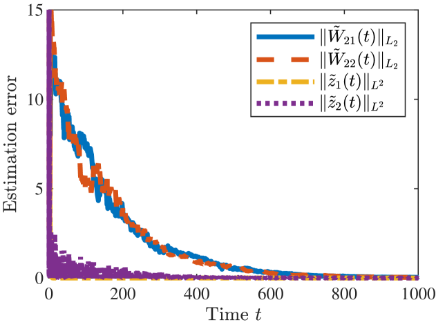
Figure 1: Evolution of the estimation errors $\|\hat{W}_{2i}(t)-W_{2i}\|_{\mathcal{L}_{2}(X,Y)}$ and $\|\hat{z}_{i}(t)-z_{i}(t)\|_{X}$ for $i\in\{1,2\}$.

(a) $t=0$

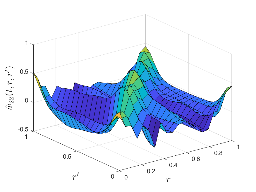
(b) $t=250$

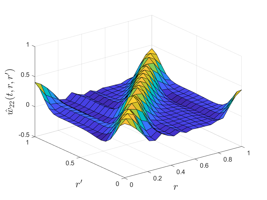
(c) $t=500$

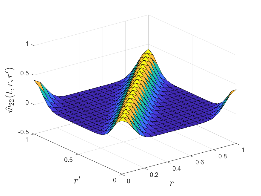
(d) $t=1000$

Figure 2: Evolution of the kernel $\hat{w}_{22}(t,r,r^{\prime})$.

6 Conclusion

In this paper, we have shown that an observer can be designed to estimate online linear operators arising in some nonlinear infinite-dimensional dynamical systems from the measurement of part of the state variables, provided that the other variables have a strongly dissipative internal dynamics. This estimation problem is motivated by an application to kernel reconstruction for neural fields equations. The main assumption is the persistence of excitation of the system along its trajectories. Our simulations suggest that this requirement can be ensured using appropriate exogenous inputs. In future works, we wish to investigate this hypothesis by either designing inputs ensuring persistency of excitation, or designing observers that do not rely on this assumption (see, e.g., [23]). Moreover, the use of this estimator in closed-loop to stabilize the systems by means of dynamic output feedback will be investigated. Finally, delayed neural fields in the form of [8] could be considered, as they do not fit into the functional setting of the present paper although capturing meaningful biological processes such as non-instantaneous axonal propagation.

References

- [1] J. Alswaihli, R. Potthast, I. Bojak, D. Saddy, and A. Hutt. Kernel reconstruction for delayed neural field equations. The Journal of Mathematical Neuroscience, 8(1):1–24, 2018.
- [2] S. Amari. Dynamics of pattern formation in lateral-inhibition type neural fields. Biological cybernetics, 27(2):77–87, 1977.
- [3] G. Besançon. Remarks on nonlinear adaptive observer design. Systems & Control Letters, 41(4):271–280, 2000.
- [4] G. Besançon and A. Ţiclea. On adaptive observers for systems with state and parameter nonlinearities. IFAC-PapersOnLine, 50(1):15416–15421, 2017. 20th IFAC World Congress.
- [5] P. Bressloff. Spatiotemporal dynamics of continuum neural fields. Journal of Physics A: Mathematical and Theoretical, 45(3), 2012.
- [6] L. Brivadis. Kernelestimation project. https://github.com/brivadis/KernelEstimation, 2021.
- [7] T. B. Burghi and R. Sepulchre. Online estimation of biophysical neural networks, 2021.
- [8] A. Chaillet, G. Detorakis, S. Palfi, and S. Senova. Robust stabilization of delayed neural fields with partial measurement and actuation. Automatica, 83:262–274, Sep. 2017.
- [9] S. Coombes, P. beim Graben, R. Potthast, and J. Wright. Neural Fields: Theory and Applications. Springer, 2014.
- [10] R. Curtain, M. Demetriou, and K. Ito. Adaptive observers for structurally perturbed infinite dimensional systems. In Proceedings of the 36th IEEE Conference on Decision and Control, volume 1, pages 509–514 vol.1, 1997.
- [11] R. Curtain, M. Demetriou, and K. Ito. Adaptive observers for slowly time varying infinite dimensional systems. In Proceedings of the 37th IEEE Conference on Decision and Control (Cat. No.98CH36171), volume 4, pages 4022–4027 vol.4, 1998.
- [12] M. A. Demetriou. Design of adaptive output feedback synchronizing controllers for networked pdes with boundary and in-domain structured perturbations and disturbances. Automatica, 90:220–229, 2018.
- [13] M. A. Demetriou and K. Ito. Adaptive observers for a class of infinite dimensional systems. IFAC Proceedings Volumes, 29(1):5346–5350, 1996. 13th World Congress of IFAC, 1996, San Francisco USA, 30 June - 5 July.
- [14] G. I. Detorakis and A. Chaillet. Incremental stability of spatiotemporal delayed dynamics and application to neural fields. In 56th IEEE Conference on Decision and Control, pages 5937–5942, 2017.
- [15] M. Farza, M. M’Saad, T. Maatoug, and M. Kamoun. Adaptive observers for nonlinearly parameterized class of nonlinear systems. Automatica, 45(10):2292–2299, 2009.
- [16] O. Faugeras, F. Grimbert, and J.-J. Slotine. Absolute stability and complete synchronization in a class of neural fields models. SIAM Journal of Applied Mathematics, 61(1):205–250, 2008.
- [17] I. Miyadera. Nonlinear semigroups, volume 109. American Mathematical Soc., 1992.
- [18] R. Potthast and P. B. Graben. Inverse problems in neural field theory. SIAM Journal on Applied Dynamical Systems, 8(4):1405–1433, 2009.
- [19] A. Pyrkin, A. Bobtsov, R. Ortega, and A. Isidori. An adaptive observer for uncertain linear time-varying systems with unknown additive perturbations, 2021.
- [20] S. Sastry, M. Bodson, and J. F. Bartram. Adaptive control: stability, convergence, and robustness, 1990.
- [21] R. E. Showalter. Monotone operators in Banach space and nonlinear partial differential equations, volume 49. American Mathematical Society, 2013.
- [22] R. Temam. Infinite-dimensional dynamical systems. Nonlinear functional analysis and its applications, Part 2, 45(Part 2):431, 1986.
- [23] J. Wang, D. Efimov, and A. A. Bobtsov. On robust parameter estimation in finite-time without persistence of excitation. IEEE Transactions on Automatic Control, 65(4):1731–1738, 2020.
- [24] H. R. Wilson and J. D. Cowan. A mathematical theory of the functional dynamics of cortical and thalamic nervous tissue. Kybernetik, 13(2):55–80, 1973.