Quaternion-based attitude stabilization via discrete-time IDA-PBC

Abstract

In this paper, we propose a new sampled-data controller for stabilization of the attitude dynamics at a desired constant configuration. The design is based on discrete-time interconnection and damping assignment (IDA) passivity-based control (PBC) and the recently proposed Hamiltonian representation of discrete-time nonlinear dynamics. Approximate solutions are provided with simulations illustrating performances.

I Introduction

Attitude stabilization aims at orienting a physical object in relation with a specified inertial frame of reference and thus it applies in several engineering contexts such as aerospace or aerial robotics. Over the past twenty years numerous continuous-time quaternion-based attitude control laws have been proposed based on several design methodologies such as feedback-linearization [1, 2], backstepping [3], sliding mode [4], optimal control or learning [5, 6]. Among these, the ones relying upon passivity-based control (PBC) are outstanding as providing, in general, simple linear control laws [7, 8, 9] in the form of P(I)D [10]. Such methods involve different parametrizations of the attitude [11] as for instance Euler angles, the Euler-Rodrigues parameters, axis-angle, etc. Among these, the ones involving quaternions are of interest and widely used motivated by the lack of singularities in general and the fact that they are computationally less intense [5, 1]. However, even if quaternions can represent all possible attitudes, this representation is not unique: each attitude corresponds to two different quaternions. This typically gives rise to undesirable phenomena such as unwinding [12, 13].

Very few results are available for addressing the design under sampling, that is when measurements are sampled and the input is piecewise constant [14]. A first solution was proposed in [15] based on sampled-data multi-rate feedback linearization. Such a solution requires a preliminary continuous-time control making the model finitely discretizable. Accordingly, if on one side such a control ensures one step convergence to the desired attitude, it requires a notable control effort and lacks in robustness with respect to unmodelled dynamics. In [16], based on the Euler-Rodrigues kinematic model, a different multi-rate digital control is designed in the context of Immersion and Invariance while relaxing the need of a preliminary continuous-time feedback. In [17], a single-rate sampled-data controller is proposed when solving a LQR problem on the approximate linear model at the desired attitude using quaternions. Such a feedback ensures local stabilization of the closed loop provided a set of LMIs is solvable off-line for a fixed value of the model parameters, the desired attitude and the sampling period.

The contribution of this work stands in providing a new scalable digital control law involving single-rate sampling and quaternion description of the kinematics. The solution we propose is based on discrete-time Interconnection and Damping Assignment (IDA)-PBC[18] over the sampled-data equivalent model associated to the attitude dynamics with the aim of assigning a suitably defined discrete port-controlled Hamiltonian (pcH) structure [19, 20]. Accordingly, the control is constructively proved to be the solution to a discrete matching equality. Even if exact closed-form solutions to this equality are tough to compute in practice, a recursive algorithm is proposed for computing approximate controllers at all desired orders. We underline that, as a byproduct and minor contribution, we also provide a new continuous-time PBC controller for attitude stabilization.

The rest of the paper is organized as follows. In Section II, the attitude control problem is recalled and solved via continuous-time PBC. In Section III, the problem is formally set in a digital context over the sampled-data equivalent model of the attitude equation. The main result is in Section IV with comparative simulations in Section V. Section VI concludes the paper with future perspectives.

Notations

Given a differentiable function $V:\mathbb{R}^{n}\to\mathbb{R}$, $\nabla V(\cdot)$ represents the gradient column-vector with $\nabla=\text{col}\{\frac{\partial}{\partial x_{i}}\}_{i={1,\dots,n}}$ and $\nabla^{2}V(\cdot)$ its Hessian. For $v,w\in\mathbb{R}^{n}$, the discrete gradient $\bar{\nabla}V|_{v}^{w}:\mathbb{R}^{n}\times\mathbb{R}^{n}\to\mathbb{R}^{n}$ is defined as

$$\bar{\nabla}V|_{v}^{w}=\int_{0}^{1}\!\nabla V(v+s(w-v))\ \textrm{d}s$$

satisfying $V(w)-V(v)=(w-v)^{\top}\bar{\nabla}V|_{v}^{w}$ with $\bar{\nabla}V|_{v}^{v}={\nabla}V(v)$. $I_{n}$ (or $I$ when clear from the context) and $I_{d}$ denote respectively the identity matrix of dimension $n$ and identity operator. $\mathbf{0}$ denotes the zero matrix of suitable dimensions. Given a smooth (i.e., infinitely differentiable) vector field $f(\cdot)$ over $\mathbb{R}^{n}$, $\mathrm{L}_{f}=\sum_{i=1}^{n}f_{i}(x)\frac{\partial}{\partial x_{i}}$ is the Lie operator with, recursively, $\mathrm{L}^{i}_{f}=\mathrm{L}_{f}\mathrm{L}_{f}^{i-1}$ and $\mathrm{L}_{f}^{0}=I_{d}$. The exponential Lie series operator is defined as $e^{\mathrm{L}_{f}}=I_{d}+\sum_{i\geq 1}\frac{1}{i!}\mathrm{L}_{f}^{i}.$ A function $R(x,\delta):\mathcal{B}\times\mathbb{R}\to\mathbb{R}^{n}$ is said in $O(\delta^{p})$, with $p\geq 1$, if it can be written as $R(x,\delta)=\delta^{p-1}\tilde{R}(x,\delta)$ for all $x\in\mathcal{B}$ and there exist a function $\theta\in\mathcal{K}_{\infty}$ and $\delta^{*}>0$ s.t. $\forall\delta\leq\delta^{*}$, $|\tilde{R}(x,\delta)|\leq\theta(\delta)$. The symbols $>$ and $<$ denote positive and negative definite functions whereas $\prec$ and $\succ$ ($\preceq$ and $\succeq$) positive and negative (semi) definite matrices. Given a vector $\omega=\text{col}\{\omega_{x},\omega_{y},\omega_{z}\}\in\mathbb{R}^{3}$, we denote

$$S(\omega)=\begin{pmatrix}0&-\omega_{z}&\omega_{y}\\ \omega_{z}&0&-\omega_{x}\\ -\omega_{y}&\omega_{x}&0\end{pmatrix}=-S^{\top}(\omega).$$

Given two matrices $A\in\mathbb{R}^{n_{1}\times n_{2}}$ and $B\in\mathbb{R}^{m_{1}\times m_{2}}$, $A\otimes B$ denotes the Kronecker product. Given a matrix $A\in\mathbb{R}^{n\times n}$, with elements $a_{ij}\in\mathbb{R}$ (for $i,j=1,\dots,n$), $\text{vec}(A):=\text{col}\{a_{11},\dots,a_{1n},\dots,a_{n1},\dots,a_{nn}\}\in\mathbb{R}^{n^{2}}$ denotes the vectorization so that $Ab=(I\otimes b^{\top})\text{vec}(A)$ for $b\in\mathbb{R}^{n}$.

II Quaternion-based attitude equations and control: the continuous-time case

In the following, let the kinematics and dynamics of a rigid body orientation in the inertial coordinates be described by

$$\dot{q}_{0}= \frac{1}{2}S(\omega)q_{0}+\frac{1}{2}\omega q_{r},\quad\dot{q}_{r}=-\frac{1}{2}\omega^{\top}q_{0}$$ (1a)

$$M\dot{\omega}= S(\omega)M\omega+u$$ (1b)

where $q=\text{col}\{q_{0},\ q_{r}\}\in\mathbb{R}^{3}\times\mathbb{R}$ is the quaternion vector (also known as Euler parameters) verifying

$$q^{\top}q=q_{0}^{\top}q_{0}+q_{r}^{2}=1,$$ (2)

$\omega\in\mathbb{R}^{3}$ is the angular velocity, $u\in\mathbb{R}^{3}$ the input torque and $M=M^{\top}\succ 0$ the inertia matrix.

Let $q^{\star}=\text{col}\{q_{0}^{\star},q_{r}^{\star}\}$ be a desired attitude configuration. Then, the attitude control problem above can be addressed over the error quaternion defined as $\varepsilon=\text{col}\{\varepsilon_{0},\varepsilon_{r}\}$ [11]

$$\varepsilon_{0}= q_{r}q_{0}^{\star}+q_{r}^{\star}q_{0}+S(q_{0})q_{0}^{\star},\quad\varepsilon_{r}=q_{r}q_{r}^{\star}-q_{0}^{\top}q_{0}^{\star}$$

with the corresponding dynamics reading

$$\dot{\varepsilon}_{0}= \frac{1}{2}S(\omega)\varepsilon_{0}+\frac{1}{2}\omega\varepsilon_{r},\quad\dot{\varepsilon}_{r}=-\frac{1}{2}\omega^{\top}\varepsilon_{0}$$ (3a)

$$M\dot{\omega}= S(\omega)M\omega+u.$$ (3b)

Accordingly, asymptotically stabilizing $q^{\star}$ for (1) corresponds to asymptotically stabilizing (3) at the equilibrium

$$\varepsilon^{\star}=\begin{pmatrix}\mathbf{0}^{\top}&1\end{pmatrix}^{\top},\quad\omega^{\star}=\mathbf{0}.$$ (4)

Among the solutions available in continuous time, the ones relying upon PBC yield a family of linear control laws [7, 8] of the form

$$u=-\kappa_{0}\varepsilon_{0}-\kappa_{\text{di}}\omega,\quad\kappa_{0},\kappa_{\text{di}}\succ 0.$$ (5)

In the following, we endorse such controllers with an IDA-PBC specification [21]. For, we note that (3) exhibits the conservative pcH form

$$\begin{pmatrix}\dot{\varepsilon}_{0}\\ \dot{\varepsilon}_{r}\\ M\dot{\omega}\end{pmatrix}=\begin{pmatrix}\frac{1}{2}S(\omega)&\frac{1}{2}\omega&\mathbf{0}\\ -\frac{1}{2}\omega^{\top}&0&\mathbf{0}\\ \mathbf{0}&\mathbf{0}&S(\omega)\end{pmatrix}\begin{pmatrix}\varepsilon_{0}\\ \varepsilon_{r}\\ M\omega\end{pmatrix}+\begin{pmatrix}\mathbf{0}\\ 0\\ I\end{pmatrix}u$$

with quadratic Hamiltonian and interconnection matrix

$$H(\varepsilon,\omega)\!\!= \!\!\frac{1}{2}\big{(}\varepsilon^{\top}\varepsilon+\omega^{\top}M\omega),\ J(\omega)\!\!\!=\!\!\!\begin{pmatrix}\frac{1}{2}S(\omega)&\frac{1}{2}\omega&\mathbf{0}\\ -\frac{1}{2}\omega^{\top}&0&\mathbf{0}\\ \mathbf{0}&\mathbf{0}&S(\omega)\end{pmatrix}.$$

On this basis, the following result holds.

Proposition II.1

Consider the error dynamics (3) and the linear feedback (5) making (4) asymptotically stable. When $\kappa_{0}=\frac{1}{2}M^{-1},$ (5) is an IDA-PBC feedback of the form

$$\begin{split}&u_{\text{ida}}(\varepsilon,\omega)=u_{\text{es}}(\varepsilon)+u_{\text{di}}(\omega)\\ &u_{\text{es}}(\varepsilon)=-\frac{1}{2}M^{-1}\varepsilon_{0},\quad u_{\text{di}}(\omega)=-\kappa_{\text{di}}\omega\end{split}$$ (6)

assigning the closed-loop pcH form

$$\begin{pmatrix}\dot{\varepsilon}_{0}\\ \dot{\varepsilon}_{r}\\ M\dot{\omega}\end{pmatrix}=\begin{pmatrix}\frac{1}{2}S(\omega)&\frac{1}{2}\omega&\frac{1}{2}M^{-1}\\ -\frac{1}{2}\omega^{\top}&0&\mathbf{0}\\ -\frac{1}{2}M^{-1}&\mathbf{0}&S(\omega)-\kappa_{\text{di}}M^{-1}\end{pmatrix}\begin{pmatrix}\varepsilon_{0}\\ \varepsilon_{r}-1\\ M\omega\end{pmatrix}$$

with

$$H_{d}(\varepsilon,\omega)=\frac{1}{2}\Big{(}\varepsilon_{0}^{\top}\varepsilon_{0}+(\varepsilon_{r}-1)^{2}+\omega^{\top}M\omega\Big{)}$$ (7a)

$$J_{d}(\omega)=\begin{pmatrix}\frac{1}{2}S(\omega)&\frac{1}{2}\omega&\frac{1}{2}M^{-1}\\ -\frac{1}{2}\omega^{\top}&0&\mathbf{0}\\ -\frac{1}{2}M^{-1}&\mathbf{0}&S(\omega)\end{pmatrix}$$ (7b)

$$R_{d}=\begin{pmatrix}\mathbf{0}&\mathbf{0}&\mathbf{0}\\ \mathbf{0}&0&\mathbf{0}\\ \mathbf{0}&\mathbf{0}&\kappa_{\text{di}}M^{-1}\end{pmatrix}\succeq 0.$$ (7c)

Before going farther we note that, as deeply commented in [12, 22], regulation to the desired orientation is, in general, achieved when $\varepsilon(t)\to\pm\varepsilon^{\star}$. However, in the result above (and throughout the whole paper), we fix the equilibrium to stabilize as the positive one while neglecting possible unwinding phenomena whose study is left as a perspective. With this in mind and because $-\varepsilon^{\star}$ is a non-isolated equilibrium of the closed-loop dynamics, all upcoming results are intended to hold locally, unless explicitly specified.

Remark II.1

To cope with unwinding, the energy-shaping controller in (6) can be modified to assign the new energy

$$\hat{H}_{d}(\varepsilon,\omega)=\frac{1}{2}\Big{(}\varepsilon_{0}^{\top}\varepsilon_{0}+1-\varepsilon_{r}^{2}+\omega^{\top}M\omega\Big{)}$$

with local minima at $\pm\varepsilon^{\star}$. This is achieved replacing in (6)

$$\begin{split}&\hat{u}_{\text{es}}(\varepsilon)=-\varepsilon_{r}M^{-1}\varepsilon_{0}\end{split}$$

assigning the closed-loop pcH form

$$\begin{pmatrix}\dot{\varepsilon}_{0}\\ \dot{\varepsilon}_{r}\\ M\dot{\omega}\end{pmatrix}\!\!\!=\!\!\!\begin{pmatrix}\frac{1}{2}S(\omega)&0&\frac{1}{2}\varepsilon_{r}M^{-1}\\ 0&0&-\frac{1}{2}\varepsilon_{0}^{\top}M^{-1}\\ -\frac{1}{2}\varepsilon_{r}M^{-1}&\frac{1}{2}M^{-1}\varepsilon_{0}&S(\omega)-\kappa_{\text{di}}M^{-1}\end{pmatrix}\!\!\!\begin{pmatrix}\varepsilon_{0}\\ -\varepsilon_{r}\\ M\omega\end{pmatrix}.$$

However, such a feedback guarantees asymptotic stabilization of the desired attitude (associated to equilibria $\pm\varepsilon^{\star}$) provided that $\varepsilon_{r}(0)\neq 0$ or $\omega(0)\neq 0$. How to overcome such a limitation is currently under investigation.

In the following, starting from Proposition II.1, we design a piecewise constant control law driving the body to the desired orientation associated to $q^{\star}=\text{col}\{q_{0}^{\star},q_{r}^{\star}\}$.

III Sampled-data model and problem statement

Consider the system (3) and let measurements (of the state) be available at the sampling instants $t=k\delta$, with $k\geq 0$ and $\delta>0$ the sampling period, and the input be piecewise constant over time intervals of length $\delta$; i.e. we set $u(t)=u_{k}$, $t\in[k\delta,(k+1)\delta[.$ Then, we seek for a sampled-data feedback $u_{k}=\gamma(\varepsilon_{k},\omega_{k})$ making (4) asymptotically stable for the sampled-data equivalent model of (3) given by

$$\zeta^{+}(u)= \zeta+\delta F^{\delta}(\zeta,u)$$ (8)

with $\zeta=\text{col}\{\varepsilon,\omega\}$, $\zeta=\zeta_{k}$, $u=u_{k}$, $\zeta^{+}(u)=\zeta_{k+1}$ and

$$f(\zeta)= f(\varepsilon,\omega)=J(\omega)\nabla H(\varepsilon,\omega),\quad B=\begin{pmatrix}\mathbf{0}^{\top}&I\end{pmatrix}^{\top}$$

$$F^{\delta}(\zeta,u)= F^{\delta}(\varepsilon,\omega,u)=J(\omega)\nabla H(\varepsilon,\omega)+Bu$$

$$+\sum_{i>0}\frac{\delta^{i}}{(i+1)!}\mathrm{L}_{f+Bu}^{i}\Big{(}J(\omega)\nabla H(\varepsilon,\omega)+Bu\Big{)}.$$

Setting $F^{\delta}_{0}(\zeta)=F^{\delta}(\zeta,\mathbf{0})$, we denote by

$$\zeta^{+}:= \zeta^{+}(\mathbf{0})=\zeta+\delta F^{\delta}_{0}(\zeta)$$

$$g^{\delta}(\varepsilon,\omega,u)u:= F^{\delta}(\zeta,u)-F^{\delta}_{0}(\zeta)$$

the drift and controlled components associated to (8). In this setting we wish to accomplish stabilization of $\zeta^{\star}=\text{col}\{\varepsilon^{\star},\mathbf{0}\}$ as in (4) by solving a discrete-time IDA-PBC problem over the sampled-data equivalent model (8) in two steps, as formalized in [18] and recalled below.

Problem III.1 (sampled-data energy-shaping)

Design the energy-shaping control $u^{\delta}_{\text{es}}:\mathbb{R}^{4}\times\mathbb{R}^{3}\to\mathbb{R}^{3}$ so that, setting

$$u=u^{\delta}_{\text{es}}(\zeta)+v$$ (9)

the closed-loop dynamics exhibits a conservative discrete-time pcH structure [19, 20]

$$\zeta^{+}(u^{\delta}_{\text{es}}(\zeta)+v)\!\!=\!\!\zeta\!\!+\!\!\delta J^{\delta}_{d}(\zeta)\bar{\nabla}H_{d}|_{\zeta}^{\zeta^{+}(u^{\delta}_{\text{es}}(\zeta))}\!\!+\!\!\delta g^{\delta}_{d}(\zeta,v)v$$ (10)

with the new Hamiltonian (7a), discrete gradient

$$\bar{\nabla}H_{d}|_{\zeta}^{\zeta^{+}}=\frac{1}{2}P(\zeta^{+}+\zeta-2\zeta^{\star}),\quad P=\begin{pmatrix}I&\mathbf{0}\\ \mathbf{0}&M\end{pmatrix}\succ 0$$

a suitable $J^{\delta}_{d}(\zeta)=-\big{(}J^{\delta}_{d}(\zeta)\big{)}^{\top}\in\mathbb{R}^{7\times 7}$ and

$$g^{\delta}_{d}(\zeta,v)v= g^{\delta}(\zeta,u^{\delta}_{\text{es}}(\zeta)+v)(u^{\delta}_{\text{es}}(\zeta)+v)$$

$$-g^{\delta}(\zeta,u^{\delta}_{\text{es}}(\zeta))u^{\delta}_{\text{es}}(\zeta).\hfill\blacksquare$$

The solution to Problem III.1 guarantees that the closed-loop dynamics (10) possesses a stable equilibrium at (4). In addition, it is proved that (9) makes (10) lossless [23] with respect to the conjugate output

$$Y^{\delta}_{d}(\zeta,v)=\big{(}g_{d}^{\delta}(\zeta,v)\big{)}^{\top}\bar{\nabla}H|_{\zeta^{+}(u^{\delta}_{\text{es}}(\zeta))}^{\zeta^{+}(u^{\delta}_{\text{es}}(\zeta)+v)}$$ (11)

that is, it verifies the dissipation equality

$$\Delta H_{d}(\zeta)\!\!=\!\!H_{d}(\zeta^{+}(u^{\delta}_{\text{es}}(\zeta)+v))\!\!-\!\!H_{d}(\zeta)\!\!=\!\!\delta v^{\top}Y^{\delta}_{d}(\zeta,v).$$ (12)

With this in mind, attitude stabilization via IDA-PBC is achieved under damping if the problem below is solved.

Problem III.2 (sampled-data damping injection)

Seek, if any, for a damping-injection feedback $v=u^{\delta}_{\text{di}}(\zeta)$ with $u^{\delta}_{\text{di}}:\mathbb{R}^{4}\times\mathbb{R}^{3}\to\mathbb{R}^{3}$ solution to the damping equality

$$u^{\delta}_{\text{di}}(\zeta)+\kappa_{\text{di}}Y^{\delta}_{d}(\zeta,u_{\text{di}}^{\delta}(\zeta))=\mathbf{0},\quad\kappa_{\text{di}}\succ 0$$ (13)

so making $\zeta^{\star}$ asymptotically stable for (10). $\hfill\blacksquare$

IV Digital attitude stabilization via IDA-PBC

Now proceed with the design in two steps by proving, in a constructive manner, the existence of both the energy-shaping and damping-injection components of the control

$$u=u^{\delta}_{\text{ida}}(\zeta)=u^{\delta}_{\text{es}}(\zeta)+u^{\delta}_{\text{di}}(\zeta)$$ (14)

aimed at, respectively, assigning and asymptotically stabilizing the desired equilibrium with a desired energy via PBC.

IV-A Main result

As detailed in Problem III.1 the energy-shaping component is responsible for assigning the equilibrium (4) with a discrete-time pcH form (10). As proved in [19] in a purely discrete-time context, this corresponds to solving the so-called Discrete-time Matching Equation (DME) below

$$J^{\delta}_{d}(\zeta)P\Big{(}\zeta-\zeta^{\star}+\frac{\delta}{2}F^{\delta}(\zeta,u^{\delta}_{\text{es}}(\zeta))\Big{)}=F^{\delta}(\zeta,u^{\delta}_{\text{es}}(\zeta))$$ (15)

for a suitably defined skew-symmetric interconnection matrix $J^{\delta}_{d}(\zeta)\in\mathbb{R}^{7\times 7}$. The next result proves that a solution to (15) exists in the form of series expansions in powers of $\delta$ around the continuous-time counterparts in Proposition II.1.

Proposition IV.1

Consider the error dynamics (3) with sampled-data equivalent model (8) and $\zeta^{\star}=\text{col}\{\varepsilon^{\star},\mathbf{0}\}$ as in (4) the equilibrium to stabilize. Then, there exists $T^{\star}>0$ such that for all $\delta\in[0,T^{\star}[$ the DME (15) admits unique solutions $<J^{\delta}_{d}(\zeta),\ u_{\text{es}}^{\delta}(\zeta)>$ in the form of series expansions around (6)-(7b); namely, one gets

$$J_{d}^{\delta}(\zeta)= J_{d}(\omega)+\sum_{i>0}\frac{\delta^{i}}{(i+1)!}J_{d}^{i}(\zeta)$$ (16a)

$$u_{\text{es}}^{\delta}(\zeta)= u_{\text{es}}(\varepsilon)+\sum_{i>0}\frac{\delta^{i}}{(i+1)!}u_{\text{es}}^{i}(\zeta)$$ (16b)

with the superscripts ⁱ denoting the order of the term in the series expansion.

Proof:

Before going through the details of the proof we highlight that, because $J_{d}^{\delta}(\zeta)$ must be skew-symmetric, then out of $49$ elements, only $28$ must be identified; accordingly, the equality (15) is in $28+3$ unknowns. With this in mind, the proof follows from the Implicit Function Theorem rewriting (15) as a formal series equality in powers of $\delta$ in the corresponding $31$ unknowns; namely, setting for simplicity $u=u_{\text{es}}^{\delta}(\zeta)$, $\mathcal{J}=J_{d}^{\delta}(\zeta)$ and $j=\mathrm{vec}(\mathcal{J})\in\mathbb{R}^{49}$, one looks for the solutions to the equality $\mathcal{Q}(\delta,\zeta,j,u)=\mathbf{0}$ where

$$\mathcal{Q}(\delta,\zeta,j,u):=F^{\delta}(\zeta,u)-(I\otimes\bar{\nabla}^{\top}H_{d}|_{\zeta}^{\zeta^{+}(u)})j$$

admits the expansion

$$\mathcal{Q}(\delta,\zeta,j,u)=\mathcal{Q}^{0}(\zeta,j,u)+\sum_{i>0}\frac{\delta^{i}}{(i+1)!}\mathcal{Q}^{i}(\zeta,j,u).$$

for suitably defined terms $\mathcal{Q}^{i}(\zeta,j,u)$ of order $i\geq 0$. Because

$$\mathcal{Q}^{0}(\zeta,j,u)= f(\zeta)+Bu-\mathcal{J}\nabla H_{d}(\zeta)$$

$$= f(\zeta)+Bu-(I\otimes\nabla^{\top}H_{d}(\zeta))j,$$

one gets that the corresponding equality $\mathcal{Q}^{0}(\zeta,j,u)=\mathbf{0}$ is solved when $j=\text{vec}(J_{d}(\omega))$ (i.e., $\mathcal{J}=J_{d}(\omega)$) and $u=u_{\text{es}}(\varepsilon)$ as in (6)-(7b). By the Implicit Function Theorem then, the formal equality $\mathcal{Q}(\delta,\zeta,j,u)=\mathbf{0}$ admits a solution of the form (16) because the matrix

$$\lim_{\delta\to 0}\begin{pmatrix}\frac{\partial}{\partial u}&\frac{\partial}{\partial j}\end{pmatrix}\mathcal{Q}(\delta,\zeta,j,u)=\begin{pmatrix}B&I\otimes\nabla^{\top}H_{d}(\zeta)\end{pmatrix}$$

$$=\begin{pmatrix}\mathbf{0}&I_{4}\otimes(\zeta-\zeta^{\star})^{\top}P&\mathbf{0}\\ I_{3}&\mathbf{0}&I_{3}\otimes(\zeta-\zeta^{\star})^{\top}P\end{pmatrix}$$

is full rank at $\zeta\neq\zeta^{\star}$ so getting the result. ∎

By the result above, the feedback law (9) assigns the conservative discrete pcH structure (10) with interconnection matrix of the form (16a) and the same Hamiltonian as in continuous time. As a consequence [19], the controlled system is passive (and lossless) with an equilibrium at the desired $\zeta^{\star}=\text{\{}\varepsilon^{\star},\mathbf{0}\}$. Accordingly, if one is able to compute a solution to the damping equality (13) asymptotic stabilization of the desired equilibrium is achieved.

Theorem IV.1

Consider the dynamics (3) under the hypotheses of Proposition IV.1 with (9) assigning the pcH form (10). Then, the following holds:

$(i)$

the dynamics (10) is lossless with respect to the output (11) and storage function (7a), that is, the energy-balance equality (12) holds;

$(ii)$

there exists $T^{\star}>0$ such that for all $\delta\in[0,T^{\star}[$ the damping equality (13) admits a unique solution in the form of a series expansion around (6), that is

$$u_{\text{di}}^{\delta}(\zeta)=u_{\text{di}}(\omega)+\sum_{i>0}\frac{\delta^{i}}{(i+1)!}u_{\text{di}}^{i}(\zeta)$$ (17)

with ⁱ denoting the order of the term in the series expansion;

$(iii)$

the IDA-PBC feedback (14) asymptotically stabilizes (10) at the desired equilibrium (4).

Proof:

$(i)$ follows by computing the one step increment of the Hamiltonian (7a) along (10); namely under Proposition IV.1 one gets

$$\Delta H_{d}= H_{d}(\zeta^{+}(u^{\delta}_{\text{es}}(\zeta)+v))-H_{d}(\zeta^{+}(u^{\delta}_{\text{es}}(\zeta)))$$

$$+H_{d}(\zeta^{+}(u^{\delta}_{\text{es}}(\zeta)))-H_{d}(\zeta)$$

$$= H_{d}(\zeta^{+}(u^{\delta}_{\text{es}}(\zeta)+v))-H_{d}(\zeta^{+}(u^{\delta}_{\text{es}}(\zeta)))$$

because $J_{d}^{\delta}(\zeta)=-\big{(}J_{d}^{\delta}(\zeta)\big{)}^{\top}$ and

$$H_{d}(\zeta^{+}(u^{\delta}_{\text{es}}(\zeta)))-H_{d}(\zeta)$$

$$=\bar{\nabla}^{\top}H_{d}|_{\zeta}^{\zeta^{+}(u^{\delta}_{\text{es}}(\zeta))}J_{d}^{\delta}(\zeta)\bar{\nabla}H_{d}|_{\zeta}^{\zeta^{+}(u^{\delta}_{\text{es}}(\zeta))}=0$$

so that

$$\Delta H_{d}=\delta\bar{\nabla}^{\top}H_{d}|_{\zeta^{+}(u^{\delta}_{\text{es}}(\zeta))}^{\zeta^{+}(u^{\delta}_{\text{es}}(\zeta)+v)}g^{\delta}_{d}(\zeta,v)v$$

and thus (12). $(ii)$ follows from the implicit function theorem along the lines of the proof of Proposition IV.1. As far as $(iii)$ is concerned, because (17) solves (13), it guarantees

$$\Delta H_{d}=-\delta\kappa_{\text{di}}\|Y^{\delta}(\zeta,u_{\text{di}}^{\delta}(\zeta))\|^{2}\leq 0,\quad\kappa_{\text{di}}\succ 0$$

with trajectories of the closed-loop system converging to the largest invariant set contained in $\{\zeta\in\mathbb{R}^{7}\text{ s.t. }Y^{\delta}(\zeta,u_{\text{di}}^{\delta}(\zeta))=0\}$. By Proposition II.1 and average passivity [23] such set only contains $\zeta^{\star}$ and $(iii)$ follows. ∎

Remark IV.1

As $\delta\to 0$, the overall attitude control law (14) and the sampled-data interconnection matrix (16) recover the continuous-time counterparts in (6) and (7b).

It turns out that the overall feedback law (14) gets the form of an asymptotic series expansion in powers of $\delta$ through the energy-shaping and damping components (16b) and (17). Despite computing closed form solutions is a tough task, approximations can be naturally defined as detailed below.

Remark IV.2

In both Theorem IV.1 and Proposition IV.1 the existence of $T^{\star}$ depends on the state at the current time; namely, for each measured state at time $t=k\delta$ (i.e., $\zeta_{k}$), there exists $T^{\star}$ so that the corresponding equalities admit a solution. Current work is toward the definition of additional uniformity arguments for the qualitative definition of a single $T^{\star}$ for all $\zeta$ in a neighborhood of $\zeta^{\star}$.

IV-B Computational aspects

The result in Proposition IV.1 highlights that a solution to the matching equality (15) (and thus to Problem III.1) exists in the form of a series expansion in powers of $\delta$. Despite closed forms are hard to be computed in practice, all terms $<J^{i}_{d}(\zeta),u_{\text{es}}^{i}(\zeta)>$ in (16) are explicitly computable as the solution to a set of linear equalities of the form

$$Bu^{i}_{\text{es}}(\zeta)-J^{i}_{d}(\zeta)\big{(}\zeta-\zeta^{\star})=\ell^{i}(\zeta),\quad i=0,1,\dots$$ (18)

with $\ell^{i}(\zeta)=\tilde{\ell}^{i}(\zeta,u_{\text{es}}(\zeta),J_{d}(\zeta),\dots,u_{\text{es}}^{i-1}(\zeta),J_{d}^{i-1}(\zeta))$ deduced by substituting (16) into (15) and equating the terms with the same powers of $\delta$. Setting blockwise

$$J_{d}^{i}(\zeta)=-\big{(}J_{d}^{i}(\zeta)\big{)}^{\top}=\begin{pmatrix}J_{11}^{i}(\zeta)&J_{12}^{i}(\zeta)&J_{13}^{i}(\zeta)\\ \star&0&J_{23}^{i}(\zeta)\\ \star&\star&J_{33}^{i}(\zeta)\end{pmatrix}$$ (19)

the solution can be iteratively computed by multiplying both sides of (18) by $B^{\perp}=\begin{pmatrix}I_{4}&\mathbf{0}\end{pmatrix}$ so getting

$$B^{\perp}J^{i}_{d}(\zeta)(\zeta-\zeta^{\star})=B^{\perp}\ell^{i}(\zeta)$$

$$u^{i}_{\text{es}}(\zeta)=B^{\top}\big{(}\ell^{i}(\zeta)+J^{i}_{d}(\zeta)(\zeta-\zeta^{\star})\big{)}$$

and, in particular, the linear equality in $J^{i}_{d}(\zeta)$ given by

$$\begin{pmatrix}J_{11}^{i}(\zeta)&J_{12}^{i}(\zeta)&J_{13}^{i}(\zeta)\\ -\big{(}J_{12}^{i}(\zeta)\big{)}^{\top}&0&J_{23}^{i}(\zeta)\end{pmatrix}\begin{pmatrix}\varepsilon_{0}\\ \varepsilon_{r}-1\\ M\omega\end{pmatrix}=B^{\perp}\ell^{i}(\zeta).$$

Accordingly, for the first terms, one gets

$$u^{1}_{\text{es}}(\zeta)= -\frac{1}{4}M^{-1}\big{(}S(\omega)q_{0}+q_{r}\omega\big{)}$$

$$u^{2}_{\text{es}}(\zeta)= \frac{3}{8}\big{(}\frac{1}{2}S(\dot{\omega}_{0})-S^{2}(\omega)\big{)}M^{-1}q_{0}+\frac{1}{2}\Big{(}\frac{1}{8}\big{(}3I$$

$$-M^{-1}\big{)}\omega\omega^{\top}-M^{-1}S(\dot{\omega}_{0})-\frac{3}{8}M^{-1}S^{2}(\omega)\Big{)}q_{0}$$

$$-\frac{3}{8}M^{-1}\dot{\omega}_{0}q_{r}$$

$J^{1}_{d}(\zeta)=J_{d}(\dot{\omega}_{0})$ and, using (19) for $i=2$$,J^{2}_{23}(\zeta)=\mathbf{0}$

$$J^{2}_{11}(\zeta)= \frac{1}{2}S(\ddot{\omega}_{0})+\frac{1}{8}M^{-1}S(\omega)M^{-1}+\frac{3}{4}S(M^{-1}u^{1}_{\text{es}}(\zeta))$$

$$-\frac{1}{6}S^{3}(\omega)+\frac{1}{2}\Big{(}S(\omega)S(\dot{\omega}_{0})-S(\dot{\omega}_{0})S(\omega)$$

$$+\omega\dot{\omega}_{0}^{\top}-\dot{\omega}_{0}^{\top}\omega\Big{)}$$

$$J^{2}_{12}(\zeta)= \frac{3}{4}M^{-1}u^{1}_{\text{es}}(\zeta)+\frac{1}{16}\omega\omega^{\top}\omega+\frac{1}{2}\ddot{\omega}_{0}$$

$$J^{2}_{13}(\zeta)= \frac{1}{16}\omega\omega^{\top}M^{-1}+\frac{1}{2}M^{-1}S^{2}(\omega)$$

$$+\frac{1}{8}\Big{(}M^{-1}S(\dot{\omega}_{0})-S(\dot{\omega}_{0})M^{-1}\Big{)}$$

$$J^{2}_{33}(\zeta)= S(\ddot{\omega}_{0})+\frac{3}{2}S(M^{-1}u^{1}_{\text{es}}(\zeta)-\frac{1}{2}S^{3}(\omega)$$

$$+\frac{1}{2}\Big{(}S(\dot{\omega}_{0})S(\omega)-S(\omega)S(\dot{\omega}_{0})\Big{)}$$

$$\dot{\omega}_{0}= M^{-1}S(\omega)M\omega-\frac{1}{2}M^{-2}q_{0}$$

$$\ddot{\omega}_{0}= M^{-1}S(\dot{\omega}_{0})M\omega+M^{-1}S(\omega)\big{(}S(\omega)M\omega\!-\!\frac{1}{2}M^{-1}\varepsilon_{0}\big{)}.$$

Along the same lines, exact forms for the damping control in Theorem IV.1 cannot be computed in practice. However, all terms of the damping injection component in (17) can be easily computed through an iterative procedure solving a linear equality in the corresponding unknown. Such an equality is deduced substituting (17) into (13) so getting, for the first terms

$$u_{\text{di}}^{1}(\zeta) =-\kappa_{\text{di}}M^{-1}\big{(}S(\omega)M-\kappa_{\text{di}}\big{)}\omega+\frac{\kappa_{\text{di}}}{2}M^{-2}\varepsilon_{0}$$

$$u_{\text{di}}^{2}(\zeta) =\dot{u}_{\text{di}}^{1}(\zeta)-\kappa_{\text{di}}M\big{(}u_{\text{es}}^{1}(\zeta)+\frac{1}{2}u_{\text{di}}^{1}(\zeta)\big{)}$$

with, recalling the continuous-time control (6),

$$\dot{u}_{\text{di}}^{1}(\zeta)= \frac{\partial u_{\text{di}}^{1}(\zeta)}{\partial\zeta}\Big{(}f(\zeta)+Bu_{\text{ida}}(\zeta)\Big{)}.$$

With this in mind, only IDA-PBC control laws defined as truncations, at all desired finite order $p\geq 0$, of the corresponding series expansions (16b) and (17) can be implemented in practice; namely, the $p^{\text{th}}$-order approximate IDA-PBC feedback is defined as

$$u^{\delta,[p]}_{\text{ida}}(\zeta)=\sum_{\ell=0}^{p}\frac{\delta^{\ell}}{(\ell+1)!}(u^{\ell}_{\text{es}}(\zeta)+u^{\ell}_{\text{di}}(\zeta)),p\geq 0.$$ (20)

For $p=0$ (20) one recovers the so-called emulation of (6), that is the continuous-time control implemented via sample-and-hold devices and no redesign taking into account the effect of sampling (see e.g., [24]). Such controllers ensure practical asymptotic stability of the desired equilibrium in closed loop [16,  Proposition 4.2]; i.e., trajectories converge to a neighborhood of the desired attitude with radius $\delta^{i+1}$.

Remark IV.3

The terms above highlight that, contrarily to the continuous-time case, the sampled-data feedback law explicitly depends on the sign of the quaternion which must be then consistently reconstructed from measurements.

22

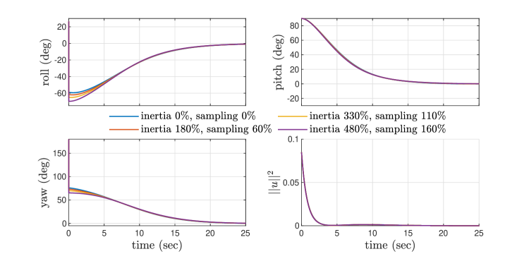
(a) Continuous-time IDA-PBC

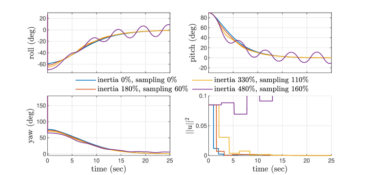
(b) $p=0$

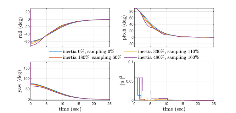
(c) $p=2$

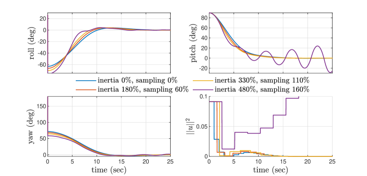
(d) Sampled-data linearized LQR

Figure 1: Stabilization results for nominal values and in presence of uncertainties

V Simulations

In this section, we consider an attitude maneuver toward $q_{0}^{\star}=\mathbf{0}$ of a rigid body having inertia matrix

$$M=\begin{pmatrix}1.42&0.00867&0.01357\\ 0.00867&1.73&0.06016\\ 0.01357&0.06016&2.03\end{pmatrix},$$ (21)

assuming initial $\omega(0)=\mathbf{0}$ and roll, pitch, yaw angles $(\phi,\psi,\theta)=(\frac{\pi}{4},\frac{\pi}{2},\pi)$ (corresponding to $q_{0}(0)=(-0.6533,0.2706,0.6533)^{\top}$ and $q_{r}(0)=0.2706$), and $\delta=1$. For the sake of comparison, in the simulations we have considered percentages of uncertainties arising in the elements $M_{22},M_{23},M_{32}$ of the inertia matrix (21) and in the sampling period $\delta$. In particular, simulations in Fig. 1 show the behaviour of the continuous-time controller (6), for $\kappa_{\text{di}}=\operatorname{diag}(1.1,0.7,0.9)$, and compared with the sampled-data controller (20) for different approximation orders (such as $p=0$ and $p=2$), and the sampled LQR control in [17].

Fig. 1 highlights that although in the nominal case all the controllers achieve $q_{0}^{\star}$ with similar performances, as uncertainties occur into the model all the controllers behave differently. In particular, the continuous-time IDA-PBC shows a robust behaviour also with respect to large uncertainties as depicted in Fig. 1a. Differently, both the sampled-data emulation design, i.e. (20) with $p=0$ (Fig. 1b), and the sampled LQR (Fig. 1d) show a significantly reduced robusteness to parametric uncertainties leading to instability for large uncertainties in both the sampling period and the inertia matrix. Finally, as readily seen in Fig. 1c, the sensitivity to uncertainty is reduced when considering two correcting terms in the sampled-data emulation design, i.e. (20) with $p=2$. In fact, the sampled-data controller with $p=2$ shows in all situations comparable performance with the continuous-time one and achieves stabilization even for larger uncertainties.

VI Conclusions and perspectives

A new quaternion-based digital control for attitude stabilizationhas been proposed. The solution involves, for the first time, discrete-time IDA-PBC over the sampled-data equivalent model so providing, in principle, a simple controller exploiting the physical properties of the dynamics. The feedback gets the form of a series expansion in powers of $\delta$ so that approximations can be naturally and efficiently applied in practice. Future works involve the case of input delays and the extension to formation control of swarms of satellites [25]. Also, the extension of IDA-PBC for general representations of the kinematics is undergoing so to cope with unwinding or singularity phenomena typically rising with parametrizations [12].

References

- [1] S.-J. Kim, C.-K. Ryoo, and K. Choi, “Robust attitude control via quaternion feedback linearization,” in SICE Annual Conference 2007. IEEE, 2007, pp. 2234–2239.
- [2] M. Navabi and M. Hosseini, “Spacecraft quaternion based attitude input-output feedback linearization control using reaction wheels,” in 2017 8th International Conference on Recent Advances in Space Technologies (RAST). IEEE, 2017, pp. 97–103.
- [3] A. Mino, K. Uchiyama, and K. Masuda, “Backstepping control for satellite attitude control using spherical control moment gyro,” in 2019 SICE International Symposium on Control Systems (SICE ISCS). IEEE, 2019, pp. 39–42.
- [4] Z. Zhu, Y. Xia, and M. Fu, “Adaptive sliding mode control for attitude stabilization with actuator saturation,” IEEE Transactions on Industrial Electronics, vol. 58, no. 10, pp. 4898–4907, 2011.
- [5] J.-Y. Wen and K. Kreutz-Delgado, “The attitude control problem,” IEEE Transactions on Automatic control, vol. 36, no. 10.
- [6] H. Hassrizal and J. Rossiter, “A survey of control strategies for spacecraft attitude and orientation,” in 2016 UKACC 11th international conference on control (CONTROL). IEEE, 2016, pp. 1–6.
- [7] F. Lizarralde and J. T. Wen, “Attitude control without angular velocity measurement: A passivity approach,” IEEE transactions on Automatic Control, vol. 41, no. 3, pp. 468–472, 1996.
- [8] P. Tsiotras, “Further passivity results for the attitude control problem,” IEEE Transactions on Automatic Control, vol. 43, no. 11.
- [9] S. Di Gennaro, “Passive attitude control of flexible spacecraft from quaternion measurements,” Journal of optimization theory and applications, vol. 116, no. 1, pp. 41–60, 2003.
- [10] M. Qasim, E. Susanto, and A. S. Wibowo, “Pid control for attitude stabilization of an unmanned aerial vehicle quad-copter,” in 2017 5th International Conference on Instrumentation, Control, and Automation (ICA). IEEE, 2017, pp. 109–114.
- [11] P. C. Hughes, Spacecraft attitude dynamics. Wiley, 2012.
- [12] S. P. Bhat and D. S. Bernstein, “A topological obstruction to continuous global stabilization of rotational motion and the unwinding phenomenon,” Systems & Control Letters, vol. 39, no. 1.
- [13] N. A. Chaturvedi, A. K. Sanyal, and N. H. McClamroch, “Rigid-body attitude control,” IEEE Control Systems Magazine, vol. 31, no. 3.
- [14] S. Monaco and D. Normand-Cyrot, “Advanced tools for nonlinear sampled-data systems’ analysis and control,” European journal of control, vol. 13, no. 2-3, pp. 221–241, 2007.
- [15] S. Monaco, D. Normand-Cyrot, and S. Stornelli, “On the linearizing feedback in nonlinear sampled data control schemes,” in 1986 25th IEEE Conference on Decision and Control, 1986, pp. 2056–2060.
- [16] M. Mattioni, S. Monaco, and D. Normand-Cyrot, “Immersion and invariance stabilization of strict-feedback dynamics under sampling,” Automatica, vol. 76, pp. 78–86, 2017.
- [17] B. Jiang, Y. Liu, and K. I. Kou, “Sampled-data control for spacecraft attitude control systems based on a quaternion model,” in 2017 Chinese Automation Congress (CAC). IEEE, 2017, pp. 4297–4300.
- [18] A. Moreschini, M. Mattioni, S. Monaco, and D. Normand-Cyrot, “Stabilization of discrete port-hamiltonian dynamics via interconnection and damping assignment,” IEEE Control Systems Letters, vol. 5, no. 1, pp. 103–108, 2020.
- [19] ——, “Discrete port-controlled Hamiltonian dynamics and average passivation,” in 58th IEEE Conference on Decision and Control (CDC), 2019, pp. 1430–1435.
- [20] S. Monaco, D. Normand-Cyrot, M. Mattioni, and A. Moreschini, “Nonlinear hamiltonian systems under sampling,” IEEE Transactions on Automatic Control, pp. 1–1, 2022.
- [21] R. Ortega, A. Van Der Schaft, B. Maschke, and G. Escobar, “Interconnection and damping assignment passivity-based control of port-controlled Hamiltonian systems,” Automatica, vol. 38, no. 4, pp. 585–596, 2002.
- [22] F. Mazenc, S. Yang, and M. R. Akella, “Quaternion-based stabilization of attitude dynamics subject to pointwise delay in the input,” Journal of Guidance, Control, and Dynamics, vol. 39, no. 8, 2016.
- [23] S. Monaco and D. Normand-Cyrot, “Nonlinear average passivity and stabilizing controllers in discrete time,” Systems & Control Letters, vol. 60, no. 6, pp. 431–439, 2011.
- [24] F. Mazenc, M. Malisoff, and T. N. Dinh, “Robustness of nonlinear systems with respect to delay and sampling of the controls,” Automatica, vol. 49, no. 6, pp. 1925–1931, 2013.
- [25] J. R. Wertz, W. J. Larson, D. Kirkpatrick, and D. Klungle, Space mission analysis and design. Springer, 1999, vol. 8.