High-Dimensional Survival Analysis: Methods and Applications

Abstract

In the era of precision medicine, time-to-event outcomes such as time to death or progression are routinely collected, along with high-throughput covariates. These high-dimensional data defy classical survival regression models, which are either infeasible to fit or likely to incur low predictability due to over-fitting. To overcome this, recent emphasis has been placed on developing novel approaches for feature selection and survival prognostication. We will review various cutting-edge methods that handle survival outcome data with high-dimensional predictors, highlighting recent innovations in machine learning approaches for survival prediction. We will cover the statistical intuitions and principles behind these methods and conclude with extensions to more complex settings, where competing events are observed. We exemplify these methods with applications to the Boston Lung Cancer Survival Cohort study, one of the largest cancer epidemiology cohorts investigating the complex mechanisms of lung cancer.

1 INTRODUCTION

Survival analysis is an area of statistics where the random variate is survival time or the time until the occurrence of a specific event, which represents a qualitative change or the transition from one discrete state to another (e.g., alive to deceased). The most often studied event in biomedicine is death, though events of interest in fields ranging from sociology to industry, to engineering, to finance, to astronomy are widely encountered. The goals of survival analysis are to describe the probability of an event occurring by some time, to detect associations between risk factors and events, or to predict survival times based on informative characteristics. What distinguishes survival outcomes from other outcomes is the presence of censoring, meaning that the event of interest may not be observed for all subjects; subjects whose event times are not observed are said to be censored. In practice, the fraction of event times that are censored in a study population can be substantial, prohibiting the direct use of standard regression methods. Estimation methods in survival analysis are built around extracting information from all subjects, censored or not.

In the era of precision medicine, survival outcomes with high-throughput covariates or predictors are routinely collected. These high-dimensional data (i.e., with the number of predictors exceeding the number of observations) challenge classical survival regression models, which are either infeasible to fit or likely to incur low predictability due to over-fitting. Recent emphasis has been placed on developing novel approaches for feature selection and survival prognostication. We will review various methods that handle survival outcome data with high-dimensional predictors, highlighting recently developed machine learning approaches for survival prediction. We will also discuss recent developments for deep learning in survival settings and introduce some new deep learning techniques in the presence of competing or semi-competing outcomes. A competing risk is an event whose occurrence precludes the occurrence of another event of interest (Austin & Fine, 2017), while in a semi-competing setting, the occurrence of a non-terminal event (e.g., disease progression) is subject to a terminal event (e.g., death), but not vice versa (Haneuse & Lee, 2016). We illustrate a novel deep learning approach for prediction under semi-competing outcomes, and exemplify the method using data from the Boston Lung Cancer Survival Cohort (BLCSC), a large hospital-based cancer epidemiology cohort investigating the molecular mechanisms and clinical pathophysiology of lung cancer (Christiani, 2017).

This paper is outlined as follows. In Section 2, we provide a brief overview of some key concepts and notation in survival analysis and introduce the necessary perquisites on which much of the subsequent literature is built. In Section 3, we survey current techniques for fitting survival models with high-dimensional covariates, primarily focusing on methods that perform feature selection under sparsity assumptions. We briefly discuss ultra high-dimensional settings and introduce screening methods, and end this section with a discussion of methods for drawing valid inference with high-dimensional covariates. In Section 4, we turn to machine learning for survival prediction. We first discuss the application of common machine learning concepts in these settings, such as a support vector machines, recursive partitioning and survival trees, and ensemble learners such as random survival forests. We briefly review artificial neural networks and extend this notion to survival prediction. In Section 5, we review existing deep learning procedures for competing risk analysis, illustrate a new deep learning approach for predicting semi-competing outcomes, and work through the BLCSC study. We conclude with remarks on future work and open areas. The online Supplementary Material tabulates the reviewed methods and their available software, and presents additional simulation results.

2 NOTATION

Consider a study consisting of $n$ subjects. The outcome variable is the time to the event of interest, such as death or cancer progression. Events in other contexts can be bankruptcy, COVID-19 infection, graduation, missing a mortgage payment, etc. A time zero also needs to be set carefully, to have proper biological or practical interpretations when helping to address specific scientific questions. For instance, some common choices of time zero in medical studies include date of birth, time of diagnosis, date of randomization in a clinical trial, or first date receiving a treatment. A unique aspect of survival analysis is that the event may go unobserved for some individuals. In particular, right censoring occurs when a subject’s follow-up ends before the event can be observed (Figure 1). Though other types of censoring exist, we focus on right censoring, which happens most often in practice.

We denote the $i$th subject’s survival and censoring times respectively by $T_{i}$ and $C_{i}$ $(i=1,\ldots,n)$, which are non-negative random variates. For the $i$th subject, we observe $\boldsymbol{X}_{i}$, a $p$-vector of covariates, $Y_{i}=\min(T_{i},C_{i})$, and the event indicator $\delta_{i}=\mathbb{I}(T_{i}\leq C_{i})$, where $\mathbb{I}(\cdot)$ is an indicator function. We assume that subjects are independent from each other, and that $T_{i}\perp C_{i}$, given $\boldsymbol{X}_{i}$. Often, the goal of survival analysis is to associate $\boldsymbol{X}_{i}$ with the distribution of $T_{i}$, and, in particular, model the conditional hazard function given $\boldsymbol{X}_{i}$, i.e.,

$$\lambda(t|\boldsymbol{X}_{i})=\lim_{\Delta\rightarrow 0}\frac{1}{\Delta}\operatorname{Pr}(t\leq T_{i}<t+\Delta|T_{i}\geq t,\boldsymbol{X}_{i}),$$ (1)

which measures the instantaneous failure rate at a given time among those who are alive and with $\boldsymbol{X}_{i}$. Throughout this review, for simplicity, we assume that $\boldsymbol{X}_{i}$ is time-invariant, though in many circumstances extensions to time-dependent covariates are possible.

Figure 1: Schematic of observations for two example patients, with different entry times, over the course of a study. The event of interest, death, is observed for Patient 1, whereas Patient 2 is censored, as the patient is still alive at the end of the study.

3 HIGH-DIMENSIONAL SURVIVAL MODELS

In high-dimensional settings, it is not recommended to build prediction models with all of the available features due to the risk of over-fitting. A useful strategy is to select only the most vital features under the assumption of sparsity, meaning that most of the potential predictors are ‘unimportant,’ with nearly no effect on the outcome (Friedman et al., 2010). A key question is how to perform variable selection and estimation simultaneously, and the most widely used approaches fall under the class of regularized regression models. Regularization refers to the addition of a penalty term to the objective function, which shrinks the coefficient estimates toward zero and possibly forces some of them to be exactly zero. This mitigates over-fitting and results in parsimonious prediction models (Tibshirani, 1996).

3.1 Regularized Cox Models

The approach that dominates survival analysis in the biomedical literature is the Cox (1972) proportional hazards model, famed for presenting both a novel hazard model and a novel concept of partial likelihood. The model links the conditional hazard function (1) to $\boldsymbol{X}_{i}$ via

$$\lambda(t|\boldsymbol{X}_{i})=\lambda_{0}(t)\exp(\boldsymbol{X}_{i}^{\top}\boldsymbol{\beta}),$$

where the baseline hazard, $\lambda_{0}(t)$, is unspecified, and $\boldsymbol{\beta}=(\beta_{1},\ldots,\beta_{p})^{\top}$ is the coefficient vector of $\boldsymbol{X}_{i}$ to be estimated, with a fixed $p<n$, by maximizing the partial likelihood, i.e.,

$$PL(\boldsymbol{\beta})=\prod_{i:\delta_{i}=1}PL_{i}(\boldsymbol{\beta}),$$

with $PL_{i}(\boldsymbol{\beta})$ being the contribution for subject $i$ who is observed to die:

$$PL_{i}(\boldsymbol{\beta})=\operatorname{Pr}(\mbox{subject $i$ dies at $Y_{i}$}\ |\ \mbox{someone from }{\cal R}(Y_{i})\mbox{ dies at $Y_{i}$})=\frac{\exp(\boldsymbol{X}_{i}^{\top}\boldsymbol{\beta})}{\sum_{j\in{\cal R}(Y_{i})}\exp(\boldsymbol{X}_{j}^{\top}\boldsymbol{\beta})}$$

where ${\cal R}(Y_{i})=\{j:Y_{j}\geq Y_{i}$}. In high-dimensional settings, that is, $p>n$ and asymptotically $p$ and $n$ may both go to infinity (Zhao & Yu, 2006), directly optimizing the partial likelihood is not feasible because of over-parameterization. Instead, regularized regression adds a penalty term to the negative log partial likelihood, $\ell(\boldsymbol{\beta})$, and optimizes a penalized version of objective function:

$$-\ell(\boldsymbol{\beta})+\eta Pen(\boldsymbol{\beta}),$$

where the penalty $Pen(\boldsymbol{\beta})$ is controlled by a positive tuning parameter, $\eta$, to be selected through cross-validation. A widely recognized family of penalties is based on the $l_{q}$-norm,

$$||\boldsymbol{\beta}||_{q}=(\sum_{j=1}^{p}|\beta_{j}|^{q})^{1/q},\ q\geq 0.$$

Regularization approaches with $Pen(\boldsymbol{\beta})=||\boldsymbol{\beta}||_{2}^{2}$, known as ridge regression (Hoerl & Kennard, 1970), are applied to the Cox model, and return unique and shrunk estimates (Verweij & Van Houwelingen, 1994). However, ridge regression does not promote sparsity, as it cannot shrink individual coefficients to zero. The least absolute shrinkage and selection operator (LASSO) (Tibshirani, 1996), with $Pen(\boldsymbol{\beta})=||\boldsymbol{\beta}||_{1}$, penalizes the absolute sum of the coefficient estimates and has been routinely used for producing sparse models. Its application (Tibshirani, 1997) to survival settings, namely, Cox LASSO, has become a widely used approach for high-dimensional survival analysis by performing feature selection and estimation simultaneously (Figure 2).

Figure 2: Graphical representation of Cox LASSO with two dimensional predictors. The blue diamond represents the constraint region $|\beta_{1}|+|\beta_{2}|\leq s$ for a given $s$. $\hat{\beta}_{MPLE}$ and $\hat{\beta}_{LASSO}$ represent the maximum partial likelihood and Cox LASSO estimates, respectively, and the red ellipses are contours of the partial likelihood function. As shown, subject to the $l_{1}$ constraint, $\hat{\beta}_{LASSO}$ is shrunk to zero compared to $\hat{\beta}_{MPLE}$, and Cox LASSO estimates $\beta_{1}$ to be exactly zero.

LASSO has several notable statistical properties. It possesses model selection consistency under certain regularity conditions, in particular, the strong irrepresentable condition when $p$ grows much faster than $n$ (i.e., that the absolute sum of coefficients for the regression of any noise variable on signal variables must be strictly smaller than 1) (Zhao & Yu, 2006). It has a Bayesian interpretation by viewing $\boldsymbol{\beta}$ as having a “double exponential” prior (Tibshirani, 2009). However, as the LASSO penalty term is linear in the size of the coefficients, it leads to biased estimates, especially for the coefficients with large absolute values. To remedy this, Zhang & Lu (2007) proposed the adaptive Cox LASSO by utilizing $Pen(\boldsymbol{\beta})=\sum_{j}w_{j}|\beta_{j}|$, with smaller weights, $w_{j}$, assigned to larger coefficients and vice versa. The estimates are $\sqrt{n}$ consistent if $\sqrt{n}\eta=O(1)$ and have oracle properties if $\sqrt{n}\eta\rightarrow 0$ and $n\eta\rightarrow\infty$. When $p>n$, it was suggested to use robust estimates such as ridge regression estimates to determine the $w_{j}$’s.

Fan & Li (2002) proposed a smoothly clipped absolute deviation (SCAD) penalty, which is a quadratic spline function of $|\beta|$ with knots at $\eta$ and $\alpha\eta$. Its derivative w.r.t $|\beta|$, i.e.,

$$\eta\left\{\mathbb{I}(|\beta|\leq\eta)+\frac{(\alpha\eta-|\beta|)_{+}}{(\alpha-1)\eta}\mathbb{I}(|\beta|>\eta)\right\};\quad\alpha>2,\eta>0,$$

may more clearly show the role of the penalty in regularizing estimating equations (Fan & Li, 2002). While the SCAD penalty retains the penalization rate of LASSO for small coefficients, it relaxes the rate of penalization smoothly as the absolute value of the coefficient increases. Asymptotically, the SCAD penalty yields $\sqrt{n}$-consistent estimates (with a proper rate of $\eta$) and possesses oracle properties (if $\sqrt{n}\eta\rightarrow 0$ and $n\eta\rightarrow\infty$). Strong oracle properties for LASSO and SCAD were established in Bradic et al. (2011), which further proposed a class of nonconvex penalization procedures for the Cox model. Nonconvex regularization, including SCAD, is appealing as it obtains support recovery properties under much weaker assumptions than for $l_{1}$ penalization (Loh & Wainwright, 2017).

Another extension is the elastic net penalty for Cox models (Wu, 2012), which combines the LASSO and ridge penalties; but, unlike LASSO, is capable of selecting more predictors than the sample size (Zou & Hastie, 2005). This notion was generalized by Vinzamuri & Reddy (2013) with the kernel elastic net Cox regression model, which replaces the ridge penalty with $\boldsymbol{\beta}^{\top}\boldsymbol{\Sigma}\boldsymbol{\beta}$. Here, $\boldsymbol{\Sigma}$ is a $p\times p$ radial basis function kernel matrix of predictors, which measures pairwise similarity between predictors. This penalty is meant to encourage correlated predictors to have similar strengths on survival prediction. Other regularized Cox methods include the group Cox LASSO (Kim et al., 2012), which selects groups of related covariates as a whole, and the fused LASSO (Chaturvedi et al., 2014), which penalizes both the coefficient estimates and their successive differences for ordered features (Table 1).

Table 1: Examples of regularized Cox regression methods and their penalty terms.

Method	Penalty	Notes
Ridge	$||\boldsymbol{\beta}||_{2}^{2}$	-
LASSO	$||\boldsymbol{\beta}||_{1}$	-
Elastic Net	$\alpha||\boldsymbol{\beta}||_{1}+(1-\alpha)||\boldsymbol{\beta}||_{2}^{2}$	$0<\alpha<1$
Adaptive LASSO	$\sum_{j}w_{j}|\beta_{j}|$	$w_{j}\geq 0$
SCAD ($Pen(|\beta|)$)	$Pen^{\prime}(|\beta|)=\eta\left\{\mathbb{I}(|\beta|\leq\eta)+\frac{(\alpha\eta-|\beta|)_{+}}{(\alpha-1)\eta}\mathbb{I}(|\beta|>\eta)\right\}$	$\alpha>2,\eta>0$
Group LASSO	$\sum_{g}||\boldsymbol{\beta}_{g}||_{1}$	$\boldsymbol{\beta}_{g}=(\beta_{g1},\ldots,\beta_{gj_{g}})^{\top}$
Fused LASSO	$\sum_{j}|\beta_{j}|$ and $\sum_{j}|\beta_{j}-\beta_{j-1}|$	-

3.2 The Dantzig Selector for Survival Data

Candès & Tao (2007) proposed another type of regularized estimator known as the Dantzig selector for linear regression:

$$\boldsymbol{Y}=\boldsymbol{X}\boldsymbol{\beta}+\boldsymbol{\epsilon},$$ (2)

where $\boldsymbol{Y}$, $\boldsymbol{X}$, $\boldsymbol{\beta}$, and $\boldsymbol{\epsilon}$ are an $n\times 1$ vector of responses, an $n\times p$ covariate matrix, a $p\times 1$ vector of coefficients and an $n\times 1$ vector of zero-mean residual errors, respectively. It estimates $\boldsymbol{\beta}$ by solving

$$\begin{gathered}\min||\boldsymbol{\beta}||_{1}\\ \vspace{2ex}\text{subject to }||\boldsymbol{X}^{\top}(\boldsymbol{Y}-\boldsymbol{X}\boldsymbol{\beta})||_{\infty}\leq\eta_{Q},\\ \end{gathered}$$

where $\eta_{Q}>0$ is a tuning parameter. Empowered by linear programming, the Dantzig selector offers a useful alternative as a regularized estimating equation approach. As a dual problem of LASSO, it often produces the same solution path (Candès & Tao, 2007).

On the other hand, accelerated failure time (AFT) models have become a useful alternative to Cox models due to the ease of interpretation (Saikia & Barman, 2017). An AFT model links the (log transformed) survival time to covariates via a linear model

$$\log(T_{i})=\boldsymbol{X}_{i}^{\top}\boldsymbol{\beta}+e_{i},$$ (3)

where the $\log$ transformation ensures the parameter space of $\boldsymbol{\beta}$ is unconstrained, and the distribution of the errors, $e_{i}$, induces a distribution for $T_{i}$ (Table 2). For parametric AFT models, maximum likelihood estimation (MLE) can be used for inference. When $e_{i}$’s distribution is unspecified, the models are semi-parametric and the MLE is difficult to obtain, as the likelihood involves infinite dimensional parameters. With a fixed $p<n$, Buckley & James (1979) proposed an estimating equation approach by imputing the censored outcomes, and solving a least squares problem.

Table 2: Specifications of various parametric accelerated failure time models.

Distribution of $e_{i}$	Induced Distribution of $T_{i}$
Normal Distribution	Log-Normal Distribution
Extreme Value Distribution	Weibull Distribution
Logistic Distribution	Log-Logistic Distribution

For AFT models with high-dimensional predictors, one cannot directly apply LASSO estimation, as the objective function again involves infinite dimensional parameters. Motivated by the work of Candès & Tao (2007) for regularized least squares estimation, Li et al. (2014) used Buckley-James imputation to express AFT estimation as a least squares problem and then applied the Dantzig selector:

$$\begin{gathered}\min||\boldsymbol{\beta}||_{1}\\ \vspace{2ex}\text{subject to }||\boldsymbol{X}^{\top}\mathbf{P}_{n}\{\boldsymbol{T}^{*}(\boldsymbol{\beta})-\boldsymbol{X}\boldsymbol{\beta}\}||_{\infty}\leq\eta_{Q},\\ \end{gathered}$$

where $T_{i}^{*}(\boldsymbol{\beta})=\log(Y_{i})+(1-\delta_{i})\frac{\int_{e_{i}(\boldsymbol{\beta})}^{\infty}\hat{S}(s,\boldsymbol{\beta})ds}{\hat{S}(e_{i}(\boldsymbol{\beta}),\boldsymbol{\beta})}$ are imputed outcomes with the Kaplan-Meier estimate, $\hat{S}(\cdot,\boldsymbol{\beta})$, based on $\{e_{i}(\boldsymbol{\beta})=\log(Y_{i})-\boldsymbol{\beta}^{\top}\boldsymbol{X}_{i},\delta_{i}\},i=1,\ldots,n$, and $\boldsymbol{T}^{*}(\boldsymbol{\beta})=(T_{1}^{*}(\boldsymbol{\beta}),\ldots,T_{n}^{*}(\boldsymbol{\beta}))^{\top}$. Here, the projection matrix $\mathbf{P}_{n}=\mathbf{I}_{n}-\mbox{\boldmath$1$}\mbox{\boldmath$1$}^{\top}/n$, where $\mathbf{I}_{n}$ and $1$ are an $n\times n$ identity matrix and an $n\times 1$ vector of 1’s, is for centering covariates to avoid estimation of the intercept or the expection of $e_{i}$ in model (3). An iterative approach is necessary because this is not a linear programming problem, and, like the Dantzig selector for linear models, estimates may be biased and may not possess the oracle property.

To address this, Li et al. (2014) considered an adaptive version of Dantzig selector with data-driven weights that vary inversely with the magnitude of coefficients. They showed that the weighted Dantzig selector has model selection consistency and oracle properties. On the other hand, a Dantzig selector for the Cox model was proposed by Antoniadis et al. (2010) based on partial likelihood score equations.

Note that, in ultra high-dimensional settings where $p\gg n$, penalized variable selection methods such as those described so far may incur high computational costs, numeric instability, and poor reproducibility (Fan & Lv, 2008). As such, variable screening is a crucial first step in identifying predictive biomarkers and reducing the dimensionality of the feature space before applying regularized methods. Feature screening methods such as sure independence screen (SIS) (Fan & Lv, 2008) fit marginal regression models for each covariate one at a time, choose a threshold, and retain those covariates with magnitudes of marginal effects above the threshold. In the ultra high-dimensional survival settings, additional censoring issues need to be addressed. Recent advancements in survival feature screening have included sure independence screening (Fan et al., 2010), principled sure independent screening (Zhao & Li, 2012), score test screening (Zhao & Li, 2014), concordance-measure based screening (Ma et al., 2017), Buckley-James assisted sure screening (Liu et al., 2020), conditional screening (Kang et al., 2017, Hong et al., 2018b), integrated power density screening (Hong et al., 2018a), $L_{q}$ norm screening (Hong et al., 2020), and forward regression (Hong et al., 2019, Pijyan et al., 2020). See a focused review of survival feature screening in Hong & Li (2017).

3.3 Inference with High-Dimensional Covariates

As simultaneous estimation and inference is challenging within the high-dimensional survival framework, we review limited methods available for drawing inference in this area. More broadly, high-dimensional regression inference methods largely fall under post-selection inference and debiased LASSO estimation. Further challenges arise in that post-selection inference is conditional on the selected subset and does not account for variation in model selection. Several authors used debiased LASSO (Van de Geer et al., 2014, Javanmard & Montanari, 2014, Yu et al., 2018) to draw inference; however, these methods require estimation of the inverse of a $p\times p$ information matrix, which is a daunting task, especially when $p>n$ (Xia et al., 2021a, b).

3.3.1 Selection-Assisted Partial Regression and Smoothing (SPARES)

To address this challenge, Fei et al. (2019) proposed SPARES to draw inference for high-dimensional linear models (2) with $p>n$. Under this framework, model selection and partial regression are conducted separately on partitioned data, and multiple sample splittings or boostraps are used to account for variations in variable selection and estimation. Specifically, given data ${\cal D}=(\boldsymbol{X},\boldsymbol{Y})$ and a variable selection procedure $\mathcal{S}_{\eta}$, data are split into equally sized ${\cal D}_{1}$ and ${\cal D}_{2}$. Denote the variables selected by $\mathcal{S}_{\eta}$ on ${\cal D}_{2}$ as $S=\mathcal{S}_{\eta}({\cal D}_{2})$. On ${\cal D}_{1}=(\boldsymbol{X}^{1},\boldsymbol{Y}^{1})$ and for any $j\in\{1,\ldots,p\}$, $\boldsymbol{Y}^{1}$ is regressed on $\boldsymbol{X}^{1}_{S\cup j}$ to estimate $\beta^{0}_{j}$ by

$$\tilde{\beta}_{j}=\Big{\{}({\boldsymbol{X}^{1}_{S\cup j}}^{\top}\boldsymbol{X}^{1}_{S\cup j})^{-1}{\boldsymbol{X}^{1}_{S\cup j}}^{\top}\boldsymbol{Y}^{1}\Big{\}}_{j},$$ (4)

where $\{\cdot\}_{j}$ denotes the estimate corresponding to variable $j$. Equation (4) is termed the partial regression estimator (Fei et al., 2019). Set $\hat{\boldsymbol{\beta}}=(\tilde{\beta}_{1},\ldots,\tilde{\beta}_{p})^{\top}$. The rationale behind this idea is that, if $\operatorname{Pr}(S\supset S_{0})\rightarrow 1$, where $S_{0}$ is the true active set, the “one-time” partial regression in (4) returns a consistent estimator for $\beta^{0}_{j}$, regardless of whether $j\in S$. However, the one-time estimator is highly variable, heavily depending on ${S}$ and the specific data-split, and does not account for variation in the variables selected. To address this, data are randomly split, say, $B$ times, and partial regression are carried out over these $B$ random splits. Denote by $\hat{\boldsymbol{\beta}}^{b}$ the estimate of $\boldsymbol{\beta}$ based on the $b$th resample ($b=1,\ldots,B$). The SPARES estimator is

$$\hat{\boldsymbol{\beta}}=\frac{1}{B}\sum_{b=1}^{B}\hat{\boldsymbol{\beta}}^{b}.$$

To draw inference, a nonparametric delta method (Efron, 2014, Van der Vaart, 2000) is used to estimate the standard error of $\hat{\beta}_{j}\;(j=1,\ldots,p)$ as $\hat{\mathrm{se}}^{B}_{j}=[\sum_{i=1}^{n}\hat{\mathrm{cov}}^{2}_{ij}]^{1/2}$, where $\hat{\mathrm{cov}}_{ij}$ is the sample covariance between $I_{bi}$ and $\hat{\beta}^{b}_{j}$, with $I_{bi}$ indicating whether subject $i$ is included in the $b$th resample (used for partial regression). Approximate $95\%$ confidence intervals are given by $\hat{\beta}_{j}\pm 1.96\ \hat{\mathrm{se}}^{B}_{j}$, while a two-sided $p$-value testing $H_{0}:\beta_{j}=0$ is given by $2\times[1-\Phi(|\hat{\beta}_{j}|/\hat{\mathrm{se}}^{B}_{j})]$, where $\Phi(\cdot)$ is the distribution function of $N(0,1)$. SPARES provides a novel inference technique that converts a high-dimensional problem to a low-dimensional regression. It is valid with general selection methods, including LASSO, SCAD, screening, and boosting, as long as they possess selection consistency or the relaxed “sure screening” condition in Fei & Li (2021). Further, this approach is not sensitive to the tuning parameter $\eta$ in $\mathcal{S}_{\eta}$ and can be extended to analyze censored outcomes, as detailed below.

3.3.2 High-Dimensional Censored Quantile Regression

As opposed to the Cox and AFT models, censored quantile regression permits the effects of covariates to vary across quantile levels, thus accommodating potentially heterogeneous impacts of certain risk predictors. For $\tau\in(0,1)$, the $\tau$-th quantile is a value at or below which a $\tau$-fraction of population lies. Denote the $\tau$-th conditional quantile of $\tilde{T}=\log(T)$ given $\boldsymbol{X}_{i}$ by $Q_{\tilde{T}}(\tau|\boldsymbol{X}_{i})$. The censored quantile regression model (Powell, 1986, Portnoy, 2003) stipulates that

$$Q_{\tilde{T}}(\tau|\boldsymbol{X}_{i})=\beta_{0}(\tau)+\boldsymbol{X}_{i}^{\top}\boldsymbol{\beta}(\tau),$$ (5)

where $\boldsymbol{\beta}(\tau)$ is a vector of quantile-specific regression coefficients. With a fixed $p<n$, Peng & Huang (2008) proposed a class of martingale-based estimating equations to estimate $\boldsymbol{\beta}(\tau)$ in model (5) over a fine grid of quantile levels, that is, $\Gamma_{m}=\{\nu=\tau_{0},\tau_{1},\ldots,\tau_{m}=\tau_{U}\}$, where $0<\tau_{U}<1$ is an upper bound for estimability. Specifically, $\boldsymbol{\beta}(\tau_{k})$’s, where $\tau_{k}\in\Gamma_{m},$ can be sequentially and consistently estimated by solving

$$\sum_{i=1}^{n}\boldsymbol{X}_{i}\left(N_{i}\left(\boldsymbol{X}_{i}^{\top}\boldsymbol{\beta}(\tau_{k})\right)-\sum_{r=0}^{k-1}\int_{\tau_{r}}^{\tau_{r+1}}\mathbb{I}[\log Y_{i}\geq\boldsymbol{X}_{i}^{\top}\check{\boldsymbol{\beta}}(\tau_{r})]dH(u)\right)=0,$$ (6)

where $N_{i}(t)=\mathbb{I}(\log Y_{i}\leq t,\delta_{i}=1)$ and $H(u)=-\log(1-u)$; see Peng & Huang (2008).

As a concrete example, with a subset of 153 patients from the BLCSC study, Hong et al. (2019) fit a censored quantile regression model that linked the conditional quantile of overall survival to age (years), sex (0: female; 1: male), pack-years, cancer type (0: adenocarcinoma; 1: non-adenocarcinoma), and cancer stage (0: stage one; 1: stage two or above). Figure 3 displays the point estimates (blue curves) of the quantile-specific regression coefficients and their 95% confidence intervals (lighter blue shaded regions).

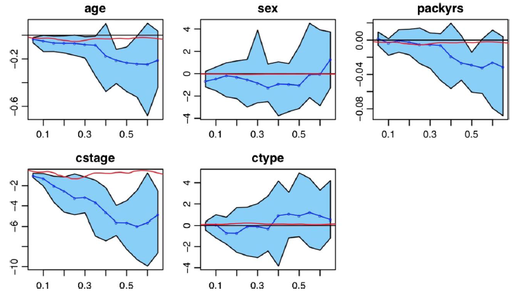
Figure 3: Example censored quantile regression analysis on $n=153$ patients from the BLCSC study. Estimated local quantile measures (Portnoy, 2003) from a Cox model are shown in red, and the reference $\beta=0$ is given in black. The figure is a permitted use of Figure 2 in Hong et al. (2019), published in Precision Clinical Medicine.

While methods have been proposed to deal with variable selection for high-dimensional censored quantile regression (HDCQR), including penalized quantile regression (Wang et al., 2013a), adaptive penalized quantile regression (Zheng et al., 2013), model-free variable screening (He et al., 2013), and stochastic integral-based estimating equations (Zheng et al., 2018), none could draw statistical inference with HDCQR. Belloni et al. (2019) provided post-selection inference in high-dimensional quantile regression at some fixed quantile levels; however, the method cannot handle censored outcomes.

To address this issue, Fei et al. (2021) proposed a Fused-HDCQR method, which utilizes a variable selection procedure for HDCQR (Zheng et al., 2018) to reduce the dimension of the data, and applies partial regression to estimate the effect of each predictor, regardless whether it is selected. Estimates are aggregated based on multiple data splits and selections. Specifically, when $p>n$, Fused-HDCQR adapts the SPARES procedure and fits low dimensional CQR’s using Equation (6). With $B$ random sample splittings, these estimates, denoted by $\tilde{\beta}_{j}^{b},b=1,\ldots,B$, are aggregated to form the Fused-HDCQR estimator:

$$\begin{gathered}\hat{\beta}_{j}(\tau_{k})=\frac{1}{B}\sum_{b=1}^{B}\tilde{\beta}_{j}^{b}(\tau_{k}),\;\tau_{k}\in\Gamma_{m}\\ \hat{\beta}_{j}(\tau)=\hat{\beta}_{j}(\tau_{k}),\;\tau_{k-1}\leq\tau<\tau_{k},\,k=1,\ldots,m,\end{gathered}$$

and a functional delta method (Van der Vaart, 2000) can be applied to estimate the variance of $\hat{\beta}_{j}(\tau_{k})$. The Fused-HDCQR procedure involves repeated fitting of low dimensional regressions, which is computationally feasible and can estimate and conduct hypothesis tests for the heterogeneous effects of various risk factors.

The use of Fused-HDCQR is illustrated with the BLCSC data by studying the differential impacts of genetic variants on different quantiles of survival times. For example, Fei et al. (2021) focused on 2,002 candidate SNPs residing in 14 well-known lung cancer related genes and investigated how each SNP played a different role among high- (i.e., lower quantiles of overall survival) versus low-risk (i.e., higher quantiles of overall survival) cancer survivors. With the Fused-HDCQR approach, the estimated coefficient of active smoking ranged from $-0.42$ ($p=0.0011$) to $-0.53$ ($p=0.0005$) as $\tau$ changed from $0.2$ to $0.5$, and then increased to $-0.31$ ($p=0.038$) as $\tau$ changed to $0.7$, suggesting that active smoking might be more harmful to the high- or median-risk groups than the low-risk group of patients. The results resonated with the strong need to develop effective smoking cession programs among high-risk populations (Barbeau et al., 2006). Further, SNP AX.37793583_T remained significant throughout $\tau=0.2$ to $\tau=0.7$, however, its estimated coefficient decreased from $2.75$ ($\tau=0.2$) to $1.39$ ($\tau=0.7$), indicating its heterogeneous impacts on survival, i.e., stronger protective effect at lower quantiles and vice versa, which could not be detected using traditional Cox models (Fei et al., 2021).

4 MACHINE LEARNING TECHNIQUES FOR SURVIVAL PREDICTION

Significant work has gone into the development of machine learning algorithms that can accommodate survival data. These nonparametric learning approaches can handle non-linear relationships or higher-order interaction that would otherwise be costly in classical methods, and can improve accuracy in prediction for survival outcomes.

4.1 Support Vector Machines

Support vector machines (SVMs) fall under the supervised learning family (Vapnik et al., 1995, Noble, 2006) and seek to find a hyperplane that provides maximal separation between groups (Figure 4). Specifically, consider a binary outcome $Y_{i}\in\{-1,1\}$ for each individual $i$ with a corresponding $p$-dimensional covariate vector, $\boldsymbol{X}_{i}$. The goal of SVM is to identify a hyperplane, $H(\psi,a)=\{\mathbf{v}\in\mathbb{R}^{p}|\langle\psi,\mathbf{v}\rangle+a=0\}$, separating these two groups so that the margin, $2/||\psi||$, can be maximized, where $\psi\in\mathbb{R}^{p}$ is the slope vector, and $\langle\cdot,\cdot\rangle$ denotes the inner product (Figure 4). Often, the two classes may not be separable in the original feature space within $\mathbb{R}^{p}$, and we use $\mathbf{F}(\cdot)$ to map the original predictors to a higher dimensional space where the outcomes can be distinguished, in which case, the hyperplane to deal with is $H(\psi,a)=\{\mathbf{v}\in\mathbb{R}^{p}|\langle\psi,\mathbf{F}(\mathbf{v})\rangle+a=0\}$ and, with slight overuse of notation, the dimension of $\psi$ is the same as that of $\mathbf{F}(\mathbf{v})$. In practice, $\mathbf{F}(\cdot)$ does not have to be obtained explicitly and $\langle\psi,\mathbf{F}(\mathbf{v})\rangle$ can be calculated by using a reproducing kernel (Wahba et al., 1999). We further introduce a slack variable, $\xi_{i}=[1-Y_{i}\{\langle\psi,\mathbf{F}(\boldsymbol{X}_{i})\rangle+a\}]_{+}$, to dictate the degree to which the $i$th data point is misclassified, as illustrated in Figure 4.

Figure 4: A support vector machine to distinguish binary outcomes with two-dimensional covariates $\mathbf{v}=(v_{1},v_{2})^{\top}$ by a linear separating line. The solid line represents the optimal hyperplane separating the data, while the dotted lines denote the maximal margin defined by the support vectors (encircled nodes) for one group (white circles) versus the other (cyan squares). Misclassified points are labeled in red, with corresponding magnitudes for slack variables, $\xi$.

SVMs have been extended to model continuous time-to-event data, which are prone to censoring, by predicting the survival time to be $\langle\psi,\mathbf{F}(\boldsymbol{X}_{i})\rangle+a$. Van Belle et al. (2007) formulated the survival SVM based on the rank concordance between the prediction and observed survival time, $Y_{i}$, among comparable individuals in the presence of censoring. Specifically, they introduced a comparability indicator, $v_{ij}=\delta_{i}\mathbb{I}(Y_{i}<Y_{j})$, such that the ordering of the observed survival times for subjects $i,j$ can only be determined when $v_{ij}=1$. For a comparable pair with $v_{ij}=1$, a concordance in rank is reached if and only if $\langle\psi,\mathbf{F}(\boldsymbol{X}_{j})\rangle-\langle\psi,\mathbf{F}(\boldsymbol{X}_{i})\rangle>0$. Allowing varying degrees of pairwise slacks, i.e., when $\langle\psi,\mathbf{F}(\boldsymbol{X}_{j})\rangle-\langle\psi,\mathbf{F}(\boldsymbol{X}_{i})\rangle\leq 0$ with $v_{ij}=1$, across comparable pairs, Van Belle et al. (2007) proposed to solve

$$\begin{split}\min_{\psi,\xi}&\frac{1}{2}\|\psi\|^{2}+\gamma\sum_{(i,j):Y_{i}<Y_{j}}v_{ij}\xi_{ij}\\ \text{ subject to }&\left\langle\psi,\mathbf{F}\left(\boldsymbol{X}_{j}\right)\right\rangle-\left\langle\psi,\mathbf{F}\left(\boldsymbol{X}_{i}\right)\right\rangle\geq-\xi_{ij},\\ \text{ and }&\xi_{ij}\geq 0,i,j=1,\ldots,n,\end{split}$$

where $\xi_{ij}$’s are pair-specific slacks, whose summation is to be minimized, and $\gamma>0$ is a regularization parameter controlling the maximal margin and misclassification penalties. This formulation can be shown to maximize the Harrell rank-based concordance index (C-index) (Harrell et al., 1982). Hence, it is termed the rank-based SVM approach for survival data and does not estimate the “intercept” $a$. An alternative regression approach (Shivaswamy et al., 2007) aimed to find a prediction, $\langle\psi,\mathbf{F}(\boldsymbol{X}_{i})\rangle+a$, for continuous survival times, by identifying a hyperplane that best fit the data that are subject to censoring (Smola & Schölkopf, 2004):

$$\begin{split}\min_{\psi,a,\xi_{,},\xi^{*}}&\frac{1}{2}\|\psi\|^{2}+\gamma\sum_{i=1}^{n}\left(\xi_{i}+\xi_{i}^{*}\right)\\ \text{ subject to }&Y_{i}-\left\langle\psi,\mathbf{F}\left(\boldsymbol{X}_{i}\right)\right\rangle-a\leq\xi_{i},\\ &\delta_{i}\left(\left\langle\psi,\mathbf{F}\left(\boldsymbol{X}_{i}\right)\right\rangle+a-Y_{i}\right)\leq\xi_{i}^{*},\\ \text{ and }&\xi_{i},\xi_{i}^{*}\geq 0.\end{split}$$

With censoring indicators incorporated into the constraints, the formulation utilizes available information from both censored and non-censored observations. To make full use of the strengths of both approaches, Van Belle et al. (2011) and Pölsterl et al. (2015) further proposed hybrid approaches, combining the penalties imposed by both methods.

4.2 Tree-Based Methods

While SVMs are adept at estimating non-linear relationships, they do not scale well for large datasets and often under-perform when the outcomes are noisy. Also there may be no clear interpretations for classifying data points above or below the estimated hyperplane (Somvanshi et al., 2016). Decision trees are an alternative for classifying patients that provide an intuitive interpretation of the hierarchical relationships between predictors. Broadly, classification and regression trees (CART) is an umbrella term for a set of recursive partitioning algorithms, which predict the group membership (classification) or target value (regression) for an observation based on a set of binary decision rules (Figure 5).

Gordon & Olshen (1985) first presented survival trees, and Ciampi et al. (1986, 1987) solidified the notion and established splitting criteria based on the log-rank and likelihood ratio test statistics, respectively, gaining predictive accuracy and interpretability. A recursive partitioning algorithm for generating a survival tree is given as follows.

1. Discretize each covariate to be a binary variable (categorical variables with $m$ levels are expressed as $m-1$ dummy variables).

2. For every binary covariate, $X_{j},\,j=1,\ldots,p$, compute the log-rank statistic to test the difference between the survival curves for the two groups defined by $X_{j}$.

3. Choose the covariate, say, $X_{j^{*}}$, with the largest significant test statistic and partition the full sample (i.e., the root node) into two groups (child nodes) based on $X_{j^{*}}$.

4. Repeat steps 2-3 for each subset (child node) until reaching the terminal nodes, that is, no covariates produce a significant test statistic and there are enough events (exceeding a prespecified number) in each terminal node.

The resulting terminal nodes split the original sample into distinct groups, who are deemed more homogeneous within each group, and will output survival estimates via Kaplan-Meier estimation in each group. Further variations in splitting are based on metrics that accommodate censored data and by either minimizing within-node homogeneity or maximizing between-node heterogeneity. For example, these metrics can be Martingale residuals (Therneau et al., 1990) or deviance residuals (LeBlanc & Crowley, 1992). With an established splitting criterion, to select a final tree, either a full survival tree is ‘grown’ and ‘pruned’ or a stopping rule is applied in backward or forward selection (Bou-Hamad et al., 2011).

Figure 5: Illustration of a classification tree with three binary covariates that yields four terminal nodes.

4.3 Ensemble Learners

While survival trees provide a fast and intuitive means of studying hierarchical relationships of predictors with outcomes, they are prone to over-fitting and high variability (Hu & Steingrimsson, 2018, Steingrimsson et al., 2016). Ensemble learners overcome the instability issues by using techniques such as bagging, boosting, and random forests.

4.3.1 Bagging

Bootstrap aggregation or bagging refers to a means of training an ensemble learner by resampling the data with replacement, training weak learners (e.g., individual survival trees) in parallel, and combining these results over the multiple bootstrapped samples (Breiman, 1996). It has three steps.

1. Bootstrapping: Resample from the original data of size $n$ with replacement to form a new sample also of size $n$, and obtain ‘$B$’ such samples.

2. Parallel Training: With each bootstrap sample, $b=1,\ldots,B$, independently train the weak learners in parallel.

3. Aggregation: Combine the $B$ individual predictions by averaging over them or by taking a majority vote.

Bagging for survival trees was first proposed by Hothorn et al. (2004); in contrast to bagging for classification trees, aggregation is done by averaging survival predictions, rather than a ‘majority vote.’ Each survival tree is grown so that every terminal node has enough events, which are used to predict the survival function node-wise at each terminal node. Then, for any newcomer, the predictions are averaged over the individual trees to yield an ensemble prediction of their survival function (Figure 6).

for tree=l sep=3em, s sep=3em, anchor=center, inner sep=0.7em, fill=cyan!20, draw=black, circle, where level=2no edge [ Training Sample, node box [Bootstrap Resampling, node box, alias=bagging, above=4em [,headcolor!70,alias=a1[[,alias=a2][]][,headcolor!70,edge label=node[above=1ex,red arrow][[][]][,headcolor!70,edge label=node[above=1ex,red arrow][,headcolor!70,edge label=node[below=1ex,red arrow]][,alias=a3]]]] [,headcolor!70,alias=b1[,headcolor!70,edge label=node[below=1ex,red arrow][[,alias=b2][]][,headcolor!70,edge label=node[above=1ex,red arrow]]][[][[][,alias=b3]]]] [  $\dots$ ,scale=2,no edge,fill=none,draw = none, yshift=-4em] [,headcolor!70,alias=c1[[,alias=c2][]][,headcolor!70,edge label=node[above=1ex,red arrow][,headcolor!70,edge label=node[above=1ex,red arrow][,alias=c3][,headcolor!70,edge label=node[above=1ex,red arrow]]][,alias=c4]]]] ] [tree box, fit=(a1)(a2)(a3)](t1); [tree box, fit=(b1)(b2)(b3)](t2); [tree box, fit=(c1)(c2)(c3)(c4)](tn); [below right=0.5em, inner sep=0pt] at (t1.north west) Tree 1; [below right=0.5em, inner sep=0pt] at (t2.north west) Tree 2; [below right=0.5em, inner sep=0pt] at (tn.north west) Tree B; t1.southwest)--tn.south east) node[midway,below=4em, node box] (mean) Aggregation; [below=3em of mean, node box] (pred) Prediction; [black arrow=5mm4mm] (bagging) – (t1.north); [black arrow] (bagging) – (t2.north); [black arrow=5mm4mm] (bagging) – (tn.north); [black arrow=5mm5mm] (t1.south) – (mean); [black arrow] (t2.south) – (mean); [black arrow=5mm5mm] (tn.south) – (mean); [black arrow] (mean) – (pred);

Figure 6: Ensemble learning with bootstrap aggregation (bagging) for survival trees.

4.3.2 Boosting

In a similar vein, boosting trains a series of weak learners with the goal of aggregating them into a better ensemble learner (Bühlmann & Hothorn, 2007). Hothorn et al. (2006) proposed a gradient boosting algorithm for survival settings. Consider a mortality risk prediction based on covariates, $\boldsymbol{X}_{i}$. For an $M$-step gradient boosting algorithm, a prediction, ${\cal F}_{m}(\boldsymbol{X}_{i})$, is made at each step, say $m=1,\ldots,M$, based on a previous prediction, ${\cal F}_{m-1}(\boldsymbol{X}_{i})$, and an additional weak learner $f_{m}(\boldsymbol{X}_{i}),$ which is the projection of the “residual error” of ${\cal F}_{m-1}(\boldsymbol{X}_{i})$ to the space spanned by $\boldsymbol{X}_{i}$,

$${\cal F}_{m}(\boldsymbol{X}_{i})={\cal F}_{m-1}(\boldsymbol{X}_{i})+w_{m}f_{m}(\boldsymbol{X}_{i}),$$

where $0<w_{m}\leq 1$ (e.g., $w_{m}=0.1$) is the step size, the residual error refers to the gradient of the loss function, e.g., the negative log partial likelihood function in a survival setting, evaluated at ${\cal F}_{m-1}(\boldsymbol{X}_{i})$, and the number of steps, $M$, can be viewed as a tuning parameter.

Boosting has two notable differences from bagging. First, boosting trains weak learners sequentially, updating the weights placed on learners iteratively, whereas in bagging individual weak learners such as survival trees are trained independently and in parallel, which are aggregated via majority voting or averaging. Second, boosting is applicable to settings where learners have low variability and high bias, as the performance is improved by redistributing the weights. In contrast, bagging is often applied when individual learners exhibit high variability, but low bias, as it reduces variations arising from individual trees.

4.3.3 Random Forests

Yet another class of ensemble learners are random forests (Breiman, 2001), which, like bagging, aggregate predictions from individual trees generated over bootstrap resampled datasets. However, differing from bagging, random forests randomly select a subset of features, say $p^{\prime}<p$ features, when generating each tree and use them for the individual tree’s growth. By doing so, random forests reduce correlations among individual trees, leading to gains in accuracy (Breiman, 2001). The choice of $p^{\prime}$ is problem-specific, which can also be viewed as a tuning parameter. In survival settings, Ishwaran et al. (2008) aggregated the survival predictions arising from each tree by averaging the predicted cumulative hazard functions into an ensemble prediction.

Further notable developments include Ishwaran et al. (2011), which extended random survival forests to high dimensions by incorporating regularization, Ishwaran & Lu (2019), which provided standard errors and confidence intervals for variable importance, and Steingrimsson et al. (2019), which proposed censoring unbiased regression trees and ensembles.

4.4 Deep Learning and Artificial Neural Networks

Deep learning has emerged as a powerful tool for risk prediction. This work stems from artificial neural networks that tried to mirror how the human brain functions (Rosenblatt, 1958), wherein nodes (or neurons) are connected in a network as a weighted sum of inputs through a series of affine transformations and non-linear activations.

A fully-connected, feed-forward artificial neural network is made up of $L$ layers, with $k_{l}$ neurons in the $l$th layer $(l=1,\ldots,L)$ (Figure 7). With an input, network predictions are made based on an $L$-fold composite function, $f_{L}\circ f_{L-1}\circ\cdots\circ f_{1}(\cdot)$ with $(g\circ f)(\cdot)=g(f(\cdot))$. At the $l$h layer, $f_{l}(\cdot)$, is defined as

$$f_{l}(\mathbf{v})=\sigma_{l}\left(\mathbf{W}_{l}\mathbf{v}+\mathbf{b}_{l}\right)\in\mathbb{R}^{k_{l}},$$

where $\mathbf{v}$ is a $k_{l-1}\times 1$ input vector fed from the $(l-1)$th layer, $\sigma_{l}(\cdot):\mathbb{R}^{k_{l}}\rightarrow\mathbb{R}^{k_{l}}$ is an activation function, $\mathbf{W}_{l}$ is a $k_{l}\times k_{l-1}$ weight matrix, $\mathbf{b}_{l}$ is a $k_{l}\times 1$ bias vector, and the $0$th layer is the input layer. Typical choices of $\sigma_{l}(\cdot)$ include the sigmoid function or the rectified linear unit activation function (ReLU), that is, $\sigma_{l}(\mathbf{b})=\max(0,\mathbf{b})$, where $\mathbf{b}\in\mathbb{R}^{k_{l}}$ and $\max(0,\cdot)$ operates component-wise.

Figure 7: Diagram of a feed-forward, fully-connected two-layer artificial neural network, including the hidden (1st) and output (2nd) layer. The input ($0$-th) layer is not counted as a real neural network layer.

For survival prediction, several deep learning approaches have emerged, beginning with the seminal work of Faraggi & Simon (1995), which adopted a fully-connected, feed-forward neural network to extend the Cox model to nonlinear predictions. Other feed-forward neural networks (Liestbl et al., 1994, Brown et al., 1997, Biganzoli et al., 1998, Eleuteri et al., 2003) used the survival status as a training label, and output predicted survival probabilities. Further developments have been made in Bayesian networks (Bellazzi & Zupan, 2008, Lisboa et al., 2003, Fard et al., 2016), convolutional neural networks (Yao et al., 2017, Katzman et al., 2016, 2018, Ranganath et al., 2016), and recurrent neural networks (Yang et al., 2018).

5 PREDICTION FOR COMPETING AND SEMI-COMPETING RISKS

Many survival processes in real applications involve multiple competing events. Risk prediction in these settings is an up-and-coming field with many potential developments. We focus on two common competing event settings, i.e., competing and semi-competing risks.

5.1 Competing Risks

In a competing risk setting, observing an event type, labeled by $c\in\{1,\ldots,K\}$, effectively eliminates the chance of observing other event types happening to the same individual (Young et al., 2020). For example, when studying the survival of patients with cancer, competing events can be cancer-related death ($c=1$) or death by cardiac disease ($c=2$) (Figure 8); an individual cannot die of cardiac disease once they have died of cancer, and vice versa. For characterizing the risk of competing events, there are two commonly used statistical metrics, namely, the cause-specific hazard and the subdistribution hazard, which target different counterfactual scenarios. The former describes the risk under hypothetical elimination of competing events, while the latter is about the observable risk without elimination of any competing events (Rudolph et al., 2020).

Figure 8: Schematic of observation times for three example patients with competing risks; $\times$: cancer death; $\times$: cardiac death; $\circ$: censoring.

Several authors (Lau et al., 2009, Koller et al., 2012) have stated that the subdistribution hazard is useful for predicting the probability of having an event of a type of interest by a given time, termed the cumulative incidence function (CIF), which reflects an individual’s actual risks and prognosis. In the following, we focus on the subdistribution hazard, which is derived from CIF, i.e., $F_{c}(t)=\operatorname{Pr}(T_{i}<t,{\cal C}_{i}=c)$, where ${\cal C}_{i}$ marks the event type for subject $i$. Specifically, for each event type $c=1,\ldots,K$, it is defined as

$$\lambda_{c}(t)=\lim_{\Delta\rightarrow 0}\frac{\operatorname{Pr}\left(t\leq T_{i}<t+\Delta,{\cal C}_{i}=c\mid T_{i}\geq t\cup\{T_{i}<t\wedge{\cal C}_{i}\neq c\}\right)}{\Delta}=\frac{dF_{c}(t)/dt}{1-F_{c}(t)},$$

which denotes the instantaneous risk of failure from event type $c$ among those who have not experienced this type of event. That is, the risk set at $t$ includes those who are event free as well as those who have experienced a competing event (other than type $c$) by $t$. The subdistribution hazard model (Fine & Gray, 1999) links a subdistribution hazard function to covariates via

$$\lambda_{c}(t|\boldsymbol{X}_{i})=\lambda_{0c}(t)\exp(\boldsymbol{X}_{i}^{\top}\boldsymbol{\beta}),$$ (7)

where $\lambda_{0c}(t)$ is the baseline subdistribution hazard function for event type $c$, and $\boldsymbol{\beta}$ specifies the effect of $\boldsymbol{X}_{i}$ on the probability of event $c$ occurring over time. In fact, model (7) implies that $1-F_{c}(t|\boldsymbol{X}_{i})=\{1-F_{0c}(t)\}^{\exp(\boldsymbol{X}_{i}^{\top}\boldsymbol{\beta})}$, where $F_{c}(t|\boldsymbol{X}_{i})$ and $F_{0c}(t)$ are the CIF given $\boldsymbol{X}_{i}$ and the baseline CIF, respectively.

With high-dimensional predictors, several authors (Kawaguchi et al., 2019, Ha et al., 2014, Ahn et al., 2018) proposed regularized subdistribution hazard models for variable selection, and Hou et al. (2019) further performed inference using a one-step debiased LASSO estimator. For prediction, several deep learning works for competing risks have been proposed based on CIFs. For example, DeepHit (Lee et al., 2018) developed a multi-task network to nonparametrically estimate $F_{c}(t|\boldsymbol{X}_{i})$ for $c=1,\ldots,K$. The network is trained to minimize a loss function, which is constructed based on the joint distribution of the first hitting time for competing events of each subject, while ensuring the concordance of estimates across subjects (Harrell et al., 1982), that is, a patient who died at a given time should have a higher risk at that time than a patient who survived longer. Dynamic DeepHit (Lee et al., 2019) further incorporated longitudinal information for dynamic predictions. Other approaches have included DeepCompete (Aastha & Liu, 2020), as well as a hierarchical approach to multi-event survival analysis (Tjandra et al., 2021).

5.2 Semi-Competing Risks

Semi-competing risk problems, a variant of competing risk problems, have commonly been encountered in clinical studies. By semi-competing, we mean that the occurrence of one event, i.e., a non-terminal event, is subject to the occurrence of another terminal event, but not vice versa (Figure 9). As the non-terminal event (e.g., cancer progression) is often a strong precursor to the terminal event (death), semi-competing events are often related and, hence, the terminal event may informatively censor the non-terminal event (Jazić et al., 2016). To overcome such informative censoring, researchers either consider only the terminal event (i.e., mortality) or a composite outcome such as progression-free survival, that is, time to progression or death, whichever comes first.

What is lacking here is how to model a predictor’s potentially different roles in disease progress and death, while utilizing the crucial information about the sojourn time between progression and death. Even in settings where the non-terminal and terminal event times are only modestly correlated, failing to acknowledge this sojourn time may lead to incorrect inference or biased predictions (Crilly et al., 2021).

Figure 9: Schematic of four example patients with semi-competing risks; $\mathbin{\blacklozenge}$: non-terminal event; $\times$: terminal event; $\circ$: censoring.

5.2.1 The Illness-Death Model

Central to the formulation of the semi-competing problem is the illness-death model, a compartment-type model for the rates at which individuals transition from being event-free (e.g., from time of diagnosis) to progression or to death or from progression to death (Andersen et al., 2012). Letting $T_{i1}$, $T_{i2}$, and $C_{i}$ denote the times to the non-terminal and terminal events, and the censoring time, respectively, we observe $(Y_{i1},\ \delta_{i1},\ Y_{i2},\ \delta_{i2},\ \boldsymbol{X}_{i}),\,i=1,\ldots,n$, where $Y_{i2}=\min(T_{i2},C_{i})$, $\delta_{i2}=\mathbb{I}(T_{i2}\leq C_{i})$, $Y_{i1}=\min(T_{i1},Y_{i2})$, $\delta_{i1}=\mathbb{I}(T_{i1}\leq Y_{i2})$, and $\boldsymbol{X}_{i}$ is a $p$-vector of covariates. The hazards for each subject at $t$ (since diagnosis) are defined and modeled as

$$\lambda_{1}\left(t\mid\gamma_{i},\boldsymbol{X}_{i}\right) =\lim_{\Delta\rightarrow 0}\frac{\operatorname{Pr}(t\leq T_{i1}<t+\Delta|T_{i1}\geq t,T_{i2}\geq t,\gamma_{i},\boldsymbol{X}_{i})}{\Delta}=\gamma_{i}\lambda_{01}\left(t\right)\exp\left\{h_{1}(\boldsymbol{X}_{i})\right\},$$ (8)

$$\lambda_{2}\left(t\mid\gamma_{i},\boldsymbol{X}_{i}\right) =\lim_{\Delta\rightarrow 0}\frac{\operatorname{Pr}(t\leq T_{i2}<t+\Delta|T_{i1}\geq t,T_{i2}\geq t,\gamma_{i},\boldsymbol{X}_{i})}{\Delta}=\gamma_{i}\lambda_{02}\left(t\right)\exp\left\{h_{2}(\boldsymbol{X}_{i})\right\},$$ (9)

$$\lambda_{3}\left(t\mid t_{1},\gamma_{i},\boldsymbol{X}_{i}\right) =\lim_{\Delta\rightarrow 0}\frac{\operatorname{Pr}(t\leq T_{i2}<t+\Delta|T_{i1}=t_{1},T_{i2}\geq t,\gamma_{i},\boldsymbol{X}_{i})}{\Delta}=\gamma_{i}\lambda_{03}\left(t-t_{1}\right)\exp\left\{h_{3}(\boldsymbol{X}_{i})\right\},$$ (10)

where $0<t_{1}<t$, and (8)-(10), respectively, correspond to the transition from diagnosis to progression prior to death, from diagnosis to death prior to progression, and from progression (that happens at $t_{1}$) to death (Haneuse & Lee, 2016). Here, $\gamma_{i}\stackrel{{\scriptstyle i.i.d}}{{\sim}}\Gamma(1/\theta,1/\theta)$ (i.e., both shape and rate are $1/\theta$ so that the mean and variance are respectively 1 and $\theta$), $i=1,\ldots,n,$ is a patient-specific frailty that models the dependence among these three transition processes within subject $i$, that is, a larger value of $\theta$ reflects a stronger dependence. In addition, $\lambda_{0g}\left(\cdot\right),g=1,2,3,$ are the baseline hazard functions for the three state transitions, respectively, and $h_{g}(\cdot),g=1,2,3,$ are log-risk functions which relate a patient’s covariates to each potential transition. The $\lambda_{0g}$ functions can be taken to be Weibull functions or piecewise constant with jumps at the distinct observed event times. Given (8)-(10), and by integrating out the frailty term, Reeder et al. (2022) derived the marginal likelihood based on $n$ independent subjects as

$$\begin{split}\mathcal{L}=\prod_{i=1}^{n}&\{\lambda_{1i}(Y_{i1})\}^{\delta_{i1}}\{\lambda_{2i}(Y_{i1})\}^{\left(1-\delta_{i1}\right)\delta_{i2}}\{\lambda_{3i}(Y_{i2}-Y_{i1})\}^{\delta_{i1}\delta_{i2}}\left(1+\theta^{-1}\right)^{\delta_{i1}\delta_{i2}}\\ &\times\left[1+\theta^{-1}\left\{\Lambda_{1i}\left(Y_{i1}\right)+\Lambda_{2i}\left(Y_{i1}\right)+\Lambda_{3i}\left(Y_{i2}-Y_{i1}\right)\right\}\right]^{-\theta-\delta_{i1}-\delta_{i2}},\end{split}$$ (11)

where $\lambda_{gi}(s)=\lambda_{0g}\left(s\right)\exp\left\{h_{g}(\boldsymbol{X}_{i})\right\}$and $\Lambda_{gi}(t)=\int_{0}^{t}\lambda_{gi}(s)ds$ for $g=1,2,3$.

5.2.2 A New Deep Learning Approach for Semi-Competing Risks

We propose a multi-task deep neural network for semi-competing risks (DNN-SCR), by using Equation (11) as the objective function with potentially high-dimensional covariates. DNN-SCR consists of three risk-specific sub-networks, respectively corresponding to the three possible state transitions, and a finite set of trainable parameters for specifying the baseline hazards (i.e., the $\phi$ parameters in Figure 10) if we specify Weibull baseline hazards, $\lambda_{0g}(s)=\phi_{g1}\phi_{g2}s^{\phi_{g2}-1}$ for $g=1,2,3,$ in (8)-(11) as well as the dependence among the three transition processes (i.e., $\theta$ in Figure 10). As opposed to the classical models, we opt for flexible, nonparametric estimation of $h_{g}(\cdot),g=1,2,3,$ to better capture potential non-linear dependencies of covariates on semi-competing events and to maximize the predictive accuracy.

In particular, we design three neural network sub-architectures to estimate the $h$ functions nonparametrically as outputs. For identifiability, we require $h_{g}(\mathbb{0})=0,g=1,2,3$, where $\mathbb{0}$ is a $p\times 1$ vector of 0’s. Each sub-network is a fully-connected feed-forward neural network with ReLU activation functions and a linear activation in the final layer (Figure 10). The numbers of hidden layers and nodes per layer as well as the dropout and learning rates are optimized as hyperparameters over a grid of values based on predictive performance. We implement our approach using the R interface for the deep learning library TensorFlow (Abadi et al., 2015), with model building and fitting done using Keras API (Chollet et al., 2015). Finite dimensional parameter training is done via the GradientTape API (Agrawal et al., 2019) for automatic differentiation. Intensive simulations have indicated the new method predicts the risks well (Supplement A).

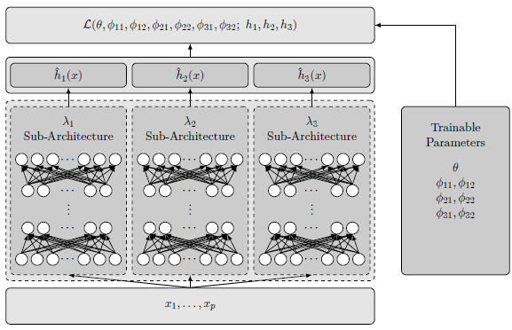
Figure 10: Architecture for the proposed semi-competing risk deep neural network.

Revisiting the BLCSC study, we exemplify our method by studying the impact of clinical and genetic predictors on disease progression and mortality. The subset includes 5,296 patients with non-small cell lung cancer, diagnosed between June 1983 and October 2021. Also included in the dataset are patients’ characteristics, namely, age at diagnosis (years), sex (0: male; 1: female), race (0: other; 1: white), ethnicity (0: non-Hispanic; 1: Hispanic), height (meters), weight (kilograms), smoking status (0: never; 1: former; 2: current), pack-years, cancer stage (1-4), and two indicators of genetic mutations (EGFR and KRAS). Semi-competing events of cancer progression and death are documented in the data; the date of progression is the date of the first source evidence, including exam, radiology report or pathology. Progression followed by death is observed in 111 (2%) patients, progression but alive at the last followup date is observed in 224 (4%) patients, and death prior to progression is observed among 1,916 (36%) patients.

To investigate the dependence of disease progression on death and predict the transition processes, we fit models (8)-(10) via a DNN-SCR. Specifically, we assume Weibull baseline hazards $\lambda_{0g}(s),g=1,2,3$, and $\gamma_{i}\stackrel{{\scriptstyle i.i.d}}{{\sim}}\Gamma(1/\theta,1/\theta)$ [as specified underneath (10)], and let $\boldsymbol{X}_{i}$ be the $i$th patient’s characteristics, $i=1,\ldots,5,296$. We then use DNN-SCR to optimize the objective function (11) in order to output the estimates of the finite dimensional parameters ($\phi$’s and $\theta$) and the predicted $h_{g},g=1,2,3$ (log risk estimates), for any covariate values.

We estimate the frailty variance, $\theta$, to be 3.15 (bootstrapped 95% CI: 3.02-3.29), suggesting that progression is indeed correlated with death. Figure 11 depicts the $h$ functions (log risks) for the effect of age at diagnosis on each state transition, stratified by sex and initial cancer stage while fixing the other covariates to be at their sample means or modes. There seems to exist a non-linear effect of age that differs by transition, cancer stage and sex. The left panel shows that younger age and more advanced stage is associated with higher hazards for progression; for the transitions from diagnosis or progression to death (the middle and right panels), older age is associated with higher hazards; interestingly, while sex does not seem to play a role in disease progression (the left panel), male patients are more likely to die than female patients after diagnosis (the middle panel) or after progression (the right panel). Finally, more advanced stage is associated with higher hazards for all the transitions.

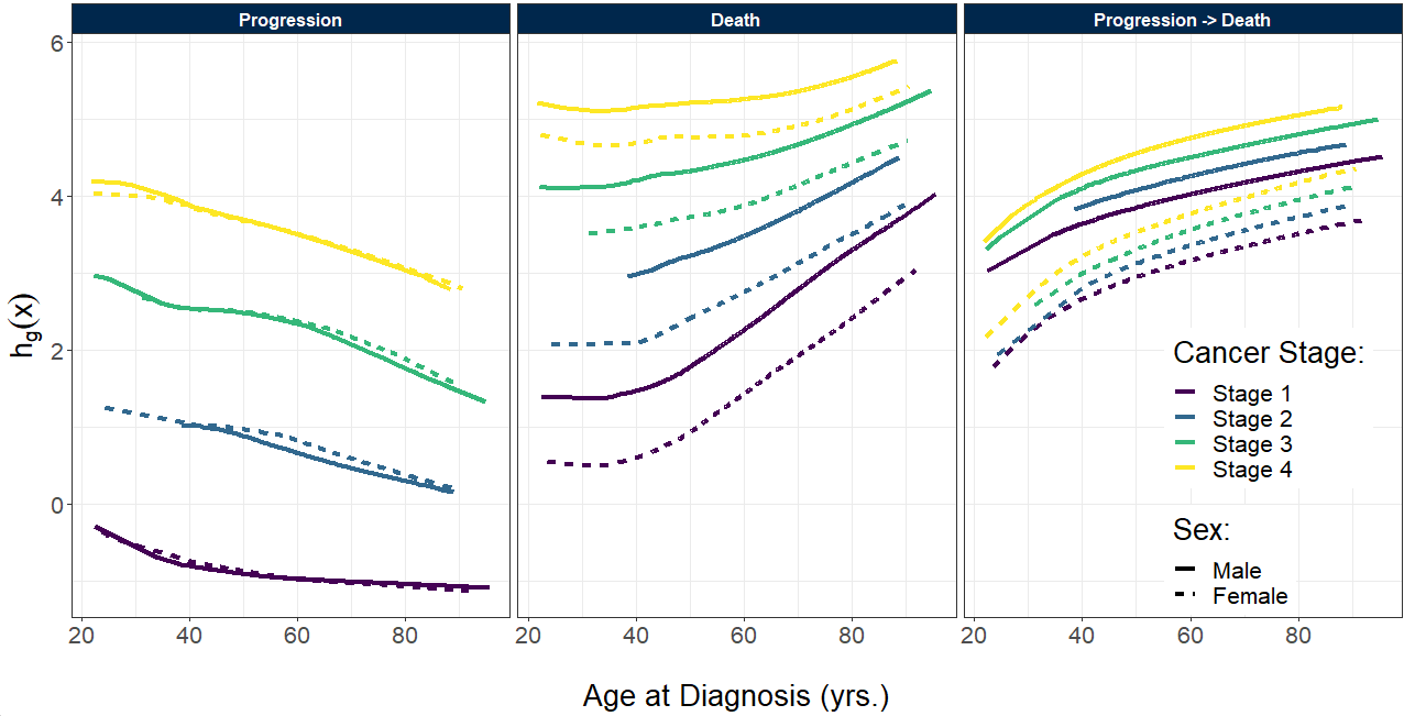
Figure 11: Log risk functions of age at diagnosis on each state transition, stratified by sex (solid versus dashed lines) and initial cancer stage (line color).

6 CONCLUSIONS

We have presented various methods for analyzing survival outcome data with high-dimensional predictors. We first provided a primer on time to event data and the unique features of survival analysis that make it distinct from other areas of statistics. We then reviewed regularization approaches for extending classical models such as the Cox, AFT, and censored quantile regression models, which lay the foundation for much of the subsequent work in this field, to high-dimensional settings. We briefly touched on feature screening for ultra high-dimensional predictors and discussed high dimensional inference with survival data. Finally, we focused on machine learning for survival prediction and concluded with methods at the forefront of the field of prognostication with competing event data.

This review is intended to provide a roadmap for readers interested in high-dimensional survival analysis (see Supplement B for tabulation of the reviewed methods and their available software), though our review is by no means exhaustive. This is an exciting and rapidly evolving field, with many open questions and new developments. For example, progress in survival predictions with high-dimensional predictors, including deep learning, active learning, and transfer learning will open new avenues to interdisciplinary breakthroughs in biomedical research and data-driven prognostic methods. Also, our review is mainly focused on frequentist methods, and in the last decade, a significant portion of Bayesian works (Lee, 2011, Annest et al., 2009, Wang et al., 2013b, Pungpapong, 2021, Bonato et al., 2011) have appeared, which make the field even more exciting. The paper pays tribute to the late Sir D.R. Cox, whose work in survival analysis has fundamentally changed the paradigm of biomedical research and will continue to impact future research for years to come.

DISCLOSURE STATEMENT

The authors declare no affiliations, memberships, funding, or financial holdings that might be perceived as affecting the objectivity of this work.

References

- Aastha & Liu (2020) Aastha PH, Liu Y. 2020. Deepcompete: A deep learning approach to competing risks in continuous time domain, In AMIA Annual Symposium Proceedings, vol. 2020, p. 177, American Medical Informatics Association
- Abadi et al. (2015) Abadi M, Agarwal A, Barham P, Brevdo E, Chen Z, et al. 2015. TensorFlow: Large-scale machine learning on heterogeneous systems. Software available from tensorflow.org
- Agrawal et al. (2019) Agrawal A, Modi A, Passos A, Lavoie A, Agarwal A, et al. 2019. Tensorflow eager: A multi-stage, python-embedded dsl for machine learning. Proceedings of Machine Learning and Systems 1:178–189
- Ahn et al. (2018) Ahn KW, Banerjee A, Sahr N, Kim S. 2018. Group and within-group variable selection for competing risks data. Lifetime Data Analysis 24(3):407–424
- Andersen et al. (2012) Andersen PK, Borgan O, Gill RD, Keiding N. 2012. Statistical models based on counting processes. Springer Science & Business Media
- Annest et al. (2009) Annest A, Bumgarner RE, Raftery AE, Yeung KY. 2009. Iterative Bayesian model averaging: A method for the application of survival analysis to high-dimensional microarray data. BMC Bioinformatics 10(1):1–17
- Antoniadis et al. (2010) Antoniadis A, Fryzlewicz P, Letué F. 2010. The Dantzig selector in Cox’s proportional hazards model. Scandinavian Journal of Statistics 37(4):531–552
- Austin & Fine (2017) Austin PC, Fine JP. 2017. Practical recommendations for reporting Fine-Gray model analyses for competing risk data. Statistics in Medicine 36(27):4391–4400
- Barbeau et al. (2006) Barbeau EM, Li Y, Calderon P, Hartman C, Quinn M, et al. 2006. Results of a union-based smoking cessation intervention for apprentice iron workers (United States). Cancer Causes & Control 17(1):53–61
- Bellazzi & Zupan (2008) Bellazzi R, Zupan B. 2008. Predictive data mining in clinical medicine: current issues and guidelines. International Journal of Medical Informatics 77(2):81–97
- Belloni et al. (2019) Belloni A, Chernozhukov V, Kato K. 2019. Valid post-selection inference in high-dimensional approximately sparse quantile regression models. Journal of the American Statistical Association 114(526):749–758
- Biganzoli et al. (1998) Biganzoli E, Boracchi P, Mariani L, Marubini E. 1998. Feed forward neural networks for the analysis of censored survival data: a partial logistic regression approach. Statistics in Medicine 17(10):1169–1186
- Bonato et al. (2011) Bonato V, Baladandayuthapani V, Broom BM, Sulman EP, Aldape KD, Do KA. 2011. Bayesian ensemble methods for survival prediction in gene expression data. Bioinformatics 27(3):359–367
- Bou-Hamad et al. (2011) Bou-Hamad I, Larocque D, Ben-Ameur H. 2011. A review of survival trees. Statistics Surveys 5:44–71
- Bradic et al. (2011) Bradic J, Fan J, Jiang J. 2011. Regularization for Cox’s proportional hazards model with np-dimensionality. Annals of Statistics 39(6):3092
- Breiman (1996) Breiman L. 1996. Bagging predictors. Machine Learning 24(2):123–140
- Breiman (2001) Breiman L. 2001. Random forests. Machine Learning 45(1):5–32
- Brown et al. (1997) Brown SF, Branford AJ, Moran W. 1997. On the use of artificial neural networks for the analysis of survival data. IEEE transactions on neural networks 8(5):1071–1077
- Buckley & James (1979) Buckley J, James I. 1979. Linear regression with censored data. Biometrika 66(3):429–436
- Bühlmann & Hothorn (2007) Bühlmann P, Hothorn T. 2007. Boosting algorithms: Regularization, prediction and model fitting. Statistical Science 22(4):477–505
- Candès & Tao (2007) Candès E, Tao T. 2007. The Dantzig selector: Statistical estimation when p is much larger than n. The Annals of Statistics 35(6):2313–2351
- Chaturvedi et al. (2014) Chaturvedi N, de Menezes RX, Goeman JJ. 2014. Fused lasso algorithm for Cox’ proportional hazards and binomial logit models with application to copy number profiles. Biometrical Journal 56(3):477–492
- Chollet et al. (2015) Chollet F, et al. 2015. Keras
- Christiani (2017) Christiani DC. 2017. The Boston lung cancer survival cohort. http://grantome.com/grant/NIH/U01-CA209414-01A1. [Online; accessed November 27, 2018]
- Ciampi et al. (1987) Ciampi A, Chang CH, Hogg S, McKinney S. 1987. Recursive partition: A versatile method for exploratory-data analysis in biostatistics. In Biostatistics. Springer, 23–50
- Ciampi et al. (1986) Ciampi A, Thiffault J, Nakache JP, Asselain B. 1986. Stratification by stepwise regression, correspondence analysis and recursive partition: a comparison of three methods of analysis for survival data with covariates. Computational Statistics & Data Analysis 4(3):185–204
- Cox (1972) Cox DR. 1972. Regression models and life tables (with discussion). Journal of the Royal Statistical Society, Series B 34(2):187–220
- Crilly et al. (2021) Crilly CJ, Haneuse S, Litt JS. 2021. Predicting the outcomes of preterm neonates beyond the neonatal intensive care unit: What are we missing? Pediatric Research 89(3):426–445
- Efron (2014) Efron B. 2014. Estimation and accuracy after model selection. Journal of the American Statistical Association 109(507):991–1007
- Eleuteri et al. (2003) Eleuteri A, Tagliaferri R, Milano L, De Placido S, De Laurentiis M. 2003. A novel neural network-based survival analysis model. Neural Networks 16(5-6):855–864
- Fan et al. (2010) Fan J, Feng Y, Wu Y. 2010. High-dimensional variable selection for Cox’s proportional hazards model. In Borrowing strength: Theory powering applications–a Festschrift for Lawrence D. Brown. Institute of Mathematical Statistics, 70–86
- Fan & Li (2002) Fan J, Li R. 2002. Variable selection for Cox’s proportional hazards model and frailty model. The Annals of Statistics 30(1):74–99
- Fan & Lv (2008) Fan J, Lv J. 2008. Sure independence screening for ultrahigh dimensional feature space. Journal of the Royal Statistical Society: Series B (Statistical Methodology) 70(5):849–911
- Faraggi & Simon (1995) Faraggi D, Simon R. 1995. A neural network model for survival data. Statistics in Medicine 14(1):73–82
- Fard et al. (2016) Fard MJ, Wang P, Chawla S, Reddy CK. 2016. A Bayesian perspective on early stage event prediction in longitudinal data. IEEE Transactions on Knowledge and Data Engineering 28(12):3126–3139
- Fei & Li (2021) Fei Z, Li Y. 2021. Estimation and inference for high dimensional generalized linear models: A splitting and smoothing approach. Journal of Machine Learning Research 22(58):1–32
- Fei et al. (2021) Fei Z, Zheng Q, Hong HG, Li Y. 2021. Inference for high-dimensional censored quantile regression. Journal of the American Statistical Association :1–15
- Fei et al. (2019) Fei Z, Zhu J, Banerjee M, Li Y. 2019. Drawing inferences for high-dimensional linear models: A selection-assisted partial regression and smoothing approach. Biometrics 75(2):551–561
- Fine & Gray (1999) Fine JP, Gray RJ. 1999. A proportional hazards model for the subdistribution of a competing risk. Journal of the American Statistical Association 94(446):496–509
- Friedman et al. (2010) Friedman J, Hastie T, Tibshirani R. 2010. Regularization paths for generalized linear models via coordinate descent. Journal of Statistical Software 33(1):1–22
- Gordon & Olshen (1985) Gordon L, Olshen RA. 1985. Tree-structured survival analysis. Cancer Treatment Reports 69(10):1065–1069
- Ha et al. (2014) Ha ID, Lee M, Oh S, Jeong JH, Sylvester R, Lee Y. 2014. Variable selection in subdistribution hazard frailty models with competing risks data. Statistics in Medicine 33(26):4590–4604
- Haneuse & Lee (2016) Haneuse S, Lee KH. 2016. Semi-competing risks data analysis: accounting for death as a competing risk when the outcome of interest is nonterminal. Circulation: Cardiovascular Quality and Outcomes 9(3):322–331
- Harrell et al. (1982) Harrell FE, Califf RM, Pryor DB, Lee KL, Rosati RA. 1982. Evaluating the yield of medical tests. JAMA 247(18):2543–2546
- He et al. (2013) He X, Wang L, Hong HG. 2013. Quantile-adaptive model-free variable screening for high-dimensional heterogeneous data. The Annals of Statistics 41(1):342–369
- Hoerl & Kennard (1970) Hoerl AE, Kennard RW. 1970. Ridge regression: Biased estimation for nonorthogonal problems. Technometrics 12(1):55–67
- Hong et al. (2020) Hong H, Chen X, Kang J, Li Y. 2020. The lq-norm learning for ultrahigh-dimensional survival data: an integrative framework. Statistica Sinica 30(3):1213
- Hong et al. (2018a) Hong HG, Chen X, Christiani DC, Li Y. 2018a. Integrated powered density: Screening ultrahigh dimensional covariates with survival outcomes. Biometrics 74(2):421–429
- Hong et al. (2019) Hong HG, Christiani DC, Li Y. 2019. Quantile regression for survival data in modern cancer research: Expanding statistical tools for precision medicine. Precision Clinical Medicine 2(2):90–99
- Hong et al. (2018b) Hong HG, Kang J, Li Y. 2018b. Conditional screening for ultra-high dimensional covariates with survival outcomes. Lifetime Data Analysis 24(1):45–71
- Hong & Li (2017) Hong HG, Li Y. 2017. Feature selection of ultrahigh-dimensional covariates with survival outcomes: a selective review. Applied Mathematics-A Journal of Chinese Universities 32(4):379–396
- Hothorn et al. (2006) Hothorn T, Bühlmann P, Dudoit S, Molinaro A, Van Der Laan MJ. 2006. Survival ensembles. Biostatistics 7(3):355–373
- Hothorn et al. (2004) Hothorn T, Lausen B, Benner A, Radespiel-Tröger M. 2004. Bagging survival trees. Statistics in Medicine 23(1):77–91
- Hou et al. (2019) Hou J, Bradic J, Xu R. 2019. Inference under fine-gray competing risks model with high-dimensional covariates. Electronic Journal of Statistics 13(2):4449–4507
- Hu & Steingrimsson (2018) Hu C, Steingrimsson JA. 2018. Personalized risk prediction in clinical oncology research: applications and practical issues using survival trees and random forests. Journal of Biopharmaceutical Statistics 28(2):333–349
- Ishwaran et al. (2008) Ishwaran H, Kogalur UB, Blackstone EH, Lauer MS. 2008. Random survival forests. The Annals of Applied Statistics 2(3):841–860
- Ishwaran et al. (2011) Ishwaran H, Kogalur UB, Chen X, Minn AJ. 2011. Random survival forests for high-dimensional data. Statistical Analysis and Data Mining: The ASA Data Science Journal 4(1):115–132
- Ishwaran & Lu (2019) Ishwaran H, Lu M. 2019. Standard errors and confidence intervals for variable importance in random forest regression, classification, and survival. Statistics in Medicine 38(4):558–582
- Javanmard & Montanari (2014) Javanmard A, Montanari A. 2014. Confidence intervals and hypothesis testing for high-dimensional regression. Journal of Machine Learning Research 15(1):2869–2909
- Jazić et al. (2016) Jazić I, Schrag D, Sargent DJ, Haneuse S. 2016. Beyond composite endpoints analysis: semicompeting risks as an underutilized framework for cancer research. JNCI: Journal of the National Cancer Institute 108(12)
- Kang et al. (2017) Kang J, Hong HG, Li Y. 2017. Partition-based ultrahigh-dimensional variable screening. Biometrika 104(4):785–800
- Katzman et al. (2016) Katzman JL, Shaham U, Cloninger A, Bates J, Jiang T, Kluger Y. 2016. Deep survival: A deep Cox proportional hazards network. Stat 1050(2):1–10
- Katzman et al. (2018) Katzman JL, Shaham U, Cloninger A, Bates J, Jiang T, Kluger Y. 2018. Deepsurv: personalized treatment recommender system using a Cox proportional hazards deep neural network. BMC Medical Research Methodology 18(1):1–12
- Kawaguchi et al. (2019) Kawaguchi ES, Shen JI, Li G, Suchard MA. 2019. A fast and scalable implementation method for competing risks data with the r package fastcmprsk. arXiv preprint arXiv:1905.07438
- Kim et al. (2012) Kim J, Sohn I, Jung SH, Kim S, Park C. 2012. Analysis of survival data with group lasso. Communications in Statistics-Simulation and Computation 41(9):1593–1605
- Koller et al. (2012) Koller MT, Raatz H, Steyerberg EW, Wolbers M. 2012. Competing risks and the clinical community: irrelevance or ignorance? Statistics in Medicine 31(11-12):1089–1097
- Lau et al. (2009) Lau B, Cole SR, Gange SJ. 2009. Competing risk regression models for epidemiologic data. American Journal of Epidemiology 170(2):244–256
- LeBlanc & Crowley (1992) LeBlanc M, Crowley J. 1992. Relative risk trees for censored survival data. Biometrics :411–425
- Lee et al. (2019) Lee C, Yoon J, Van Der Schaar M. 2019. Dynamic-deephit: A deep learning approach for dynamic survival analysis with competing risks based on longitudinal data. IEEE Transactions on Biomedical Engineering 67(1):122–133
- Lee et al. (2018) Lee C, Zame WR, Yoon J, van der Schaar M. 2018. Deephit: A deep learning approach to survival analysis with competing risks, In Thirty-second AAAI conference on artificial intelligence
- Lee (2011) Lee KH. 2011. Bayesian variable selection in parametric and semiparametric high dimensional survival analysis. University of Missouri-Columbia
- Li et al. (2014) Li Y, Dicker L, Zhao SD. 2014. The Dantzig selector for censored linear regression models. Statistica Sinica 24(1):251
- Liestbl et al. (1994) Liestbl K, Andersen PK, Andersen U. 1994. Survival analysis and neural nets. Statistics in Medicine 13(12):1189–1200
- Lisboa et al. (2003) Lisboa PJ, Wong H, Harris P, Swindell R. 2003. A Bayesian neural network approach for modelling censored data with an application to prognosis after surgery for breast cancer. Artificial intelligence in medicine 28(1):1–25
- Liu et al. (2020) Liu Y, Chen X, Li G. 2020. A new joint screening method for right-censored time-to-event data with ultra-high dimensional covariates. Statistical Methods in Medical Research 29(6):1499–1513
- Loh & Wainwright (2017) Loh PL, Wainwright MJ. 2017. Support recovery without incoherence: A case for nonconvex regularization. The Annals of Statistics 45(6):2455–2482
- Ma et al. (2017) Ma Y, Li Y, Lin H. 2017. Concordance measure-based feature screening and variable selection. Statistica Sinica 27:1967–1985
- Noble (2006) Noble WS. 2006. What is a support vector machine? Nature Biotechnology 24(12):1565–1567
- Peng & Huang (2008) Peng L, Huang Y. 2008. Survival analysis with quantile regression models. Journal of the American Statistical Association 103(482):637–649
- Pijyan et al. (2020) Pijyan A, Zheng Q, Hong HG, Li Y. 2020. Consistent estimation of generalized linear models with high dimensional predictors via stepwise regression. Entropy 22(9):965
- Pölsterl et al. (2015) Pölsterl S, Navab N, Katouzian A. 2015. Fast training of support vector machines for survival analysis, In Joint European Conference on Machine Learning and Knowledge Discovery in Databases, pp. 243–259, Springer
- Portnoy (2003) Portnoy S. 2003. Censored regression quantiles. Journal of the American Statistical Association 98(464):1001–1012
- Powell (1986) Powell JL. 1986. Censored regression quantiles. Journal of Econometrics 32(1):143–155
- Pungpapong (2021) Pungpapong V. 2021. Incorporating biological networks into high-dimensional Bayesian survival analysis using an icm/m algorithm. Journal of Bioinformatics and Computational Biology 19(05):2150027
- Ranganath et al. (2016) Ranganath R, Perotte A, Elhadad N, Blei D. 2016. Deep survival analysis, In Machine Learning for Healthcare Conference, pp. 101–114, PMLR
- Reeder et al. (2022) Reeder HT, Lu J, Haneuse S. 2022. Penalized estimation of frailty-based illness-death models for semi-competing risks. arXiv preprint arXiv:2202.00618
- Rosenblatt (1958) Rosenblatt F. 1958. The perceptron: a probabilistic model for information storage and organization in the brain. Psychological Review 65(6):386
- Rudolph et al. (2020) Rudolph JE, Lesko CR, Naimi AI. 2020. Causal inference in the face of competing events. Current Epidemiology Reports 7(3):125–131
- Saikia & Barman (2017) Saikia R, Barman MP. 2017. A review on accelerated failure time models. International Journal of Statistics and Systems 12(2):311–322
- Shivaswamy et al. (2007) Shivaswamy PK, Chu W, Jansche M. 2007. A support vector approach to censored targets, In Seventh IEEE international conference on data mining (ICDM 2007), pp. 655–660, IEEE
- Smola & Schölkopf (2004) Smola AJ, Schölkopf B. 2004. A tutorial on support vector regression. Statistics and Computing 14(3):199–222
- Somvanshi et al. (2016) Somvanshi M, Chavan P, Tambade S, Shinde SV. 2016. A review of machine learning techniques using decision tree and support vector machine, In 2016 International Conference on Computing Communication Control and automation (ICCUBEA), pp. 1–7
- Steingrimsson et al. (2016) Steingrimsson JA, Diao L, Molinaro AM, Strawderman RL. 2016. Doubly robust survival trees. Statistics in Medicine 35(20):3595–3612
- Steingrimsson et al. (2019) Steingrimsson JA, Diao L, Strawderman RL. 2019. Censoring unbiased regression trees and ensembles. Journal of the American Statistical Association 114(525):370–383
- Therneau et al. (1990) Therneau TM, Grambsch PM, Fleming TR. 1990. Martingale-based residuals for survival models. Biometrika 77(1):147–160
- Tibshirani (1996) Tibshirani RJ. 1996. Regression shrinkage and selection via the lasso. Journal of the Royal Statistical Society, Series B 58:267–288
- Tibshirani (1997) Tibshirani RJ. 1997. The lasso method for variable selection in the Cox model. Statistics in Medicine 16:385–395
- Tibshirani (2009) Tibshirani RJ. 2009. Univariate shrinkage in the Cox model for high dimensional data. Statistical Applications in Genetics and Molecular Biology 8:21
- Tjandra et al. (2021) Tjandra D, He Y, Wiens J. 2021. A hierarchical approach to multi-event survival analysis, In Proceedings of the AAAI Conference on Artificial Intelligence, vol. 35, pp. 591–599
- Van Belle et al. (2007) Van Belle V, Pelckmans K, Suykens J, Van Huffel S. 2007. Support vector machines for survival analysis, In Proceedings of the Third International Conference on Computational Intelligence in Medicine and Healthcare (CIMED2007), pp. 1–8
- Van Belle et al. (2011) Van Belle V, Pelckmans K, Van Huffel S, Suykens JA. 2011. Support vector methods for survival analysis: a comparison between ranking and regression approaches. Artificial Intelligence in Medicine 53(2):107–118
- Van de Geer et al. (2014) Van de Geer S, Bühlmann P, Ritov Y, Dezeure R. 2014. On asymptotically optimal confidence regions and tests for high-dimensional models. The Annals of Statistics 42(3):1166–1202
- Van der Vaart (2000) Van der Vaart AW. 2000. Asymptotic statistics, vol. 3. Cambridge University Press
- Vapnik et al. (1995) Vapnik V, Guyon I, Hastie T. 1995. Support vector machines. Mach. Learn 20(3):273–297
- Verweij & Van Houwelingen (1994) Verweij PJ, Van Houwelingen HC. 1994. Penalized likelihood in Cox regression. Statistics in Medicine 13(23-24):2427–2436
- Vinzamuri & Reddy (2013) Vinzamuri B, Reddy CK. 2013. Cox regression with correlation based regularization for electronic health records, In 2013 IEEE 13th International Conference on Data Mining, pp. 757–766, IEEE
- Wahba et al. (1999) Wahba G, et al. 1999. Support vector machines, reproducing kernel hilbert spaces and the randomized gacv. Advances in Kernel Methods-Support Vector Learning 6:69–87
- Wang et al. (2013a) Wang HJ, Zhou J, Li Y. 2013a. Variable selection for censored quantile regresion. Statistica Sinica 23(1):145
- Wang et al. (2013b) Wang W, Baladandayuthapani V, Morris JS, Broom BM, Manyam G, Do KA. 2013b. ibag: integrative Bayesian analysis of high-dimensional multiplatform genomics data. Bioinformatics 29(2):149–159
- Wu (2012) Wu Y. 2012. Elastic net for Cox’s proportional hazards model with a solution path algorithm. Statistica Sinica 22:27
- Xia et al. (2021a) Xia L, Nan B, Li Y. 2021a. Debiased lasso for generalized linear models with a diverging number of covariates. Biometrics doi: 10.1111/biom.13587:Online ahead of print
- Xia et al. (2021b) Xia L, Nan B, Li Y. 2021b. Statistical inference for Cox proportional hazards models with a diverging number of covariates. arXiv preprint arXiv:2106.03244
- Yang et al. (2018) Yang G, Cai Y, Reddy CK. 2018. Spatio-temporal check-in time prediction with recurrent neural network based survival analysis, In Proceedings of the Twenty-Seventh International Joint Conference on Artificial Intelligence
- Yao et al. (2017) Yao J, Zhu X, Zhu F, Huang J. 2017. Deep correlational learning for survival prediction from multi-modality data, In International Conference on Medical Image Computing and Computer-Assisted Intervention, pp. 406–414, Springer
- Young et al. (2020) Young JG, Stensrud MJ, Tchetgen Tchetgen EJ, Hernán MA. 2020. A causal framework for classical statistical estimands in failure-time settings with competing events. Statistics in Medicine 39(8):1199–1236
- Yu et al. (2018) Yu Y, Bradic J, Samworth RJ. 2018. Confidence intervals for high-dimensional Cox models. arXiv preprint arXiv:1803.01150
- Zhang & Lu (2007) Zhang HH, Lu W. 2007. Adaptive lasso for Cox’s proportional hazards model. Biometrika 94(3):691–703
- Zhao & Yu (2006) Zhao P, Yu B. 2006. On model selection consistency of lasso. Journal of Machine Learning Research 7(Nov):2541–2563
- Zhao & Li (2012) Zhao SD, Li Y. 2012. Principled sure independence screening for Cox models with ultra-high-dimensional covariates. Journal of Multivariate Analysis 105(1):397–411
- Zhao & Li (2014) Zhao SD, Li Y. 2014. Score test variable screening. Biometrics 70(4):862–871
- Zheng et al. (2013) Zheng Q, Gallagher C, Kulasekera K. 2013. Adaptive penalized quantile regression for high dimensional data. Journal of Statistical Planning and Inference 143(6):1029–1038
- Zheng et al. (2018) Zheng Q, Peng L, He X. 2018. High dimensional censored quantile regression. The Annals of Statistics 46(1):308–343
- Zou & Hastie (2005) Zou H, Hastie T. 2005. Regularization and variable selection via the elastic net. Journal of the Royal Statistical society: Series B (Statistical Methodology) 67(2):301–320