Dual Octree Graph Networks for Learning Adaptive Volumetric Shape Representations

Abstract.

We present an adaptive deep representation of volumetric fields of 3D shapes and an efficient approach to learn this deep representation for high-quality 3D shape reconstruction and auto-encoding. Our method encodes the volumetric field of a 3D shape with an adaptive feature volume organized by an octree and applies a compact multilayer perceptron network for mapping the features to the field value at each 3D position. An encoder-decoder network is designed to learn the adaptive feature volume based on the graph convolutions over the dual graph of octree nodes. The core of our network is a new graph convolution operator defined over a regular grid of features fused from irregular neighboring octree nodes at different levels, which not only reduces the computational and memory cost of the convolutions over irregular neighboring octree nodes, but also improves the performance of feature learning. Our method effectively encodes shape details, enables fast 3D shape reconstruction, and exhibits good generality for modeling 3D shapes out of training categories. We evaluate our method on a set of reconstruction tasks of 3D shapes and scenes and validate its superiority over other existing approaches. Our code, data, and trained models are available at https://wang-ps.github.io/dualocnn.

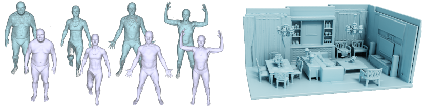
Figure 1. 3D reconstruction results generated by our dual octree graph network trained on raw scans of human bodies from the D-Faust dataset (Bogo et al., 2017) via unsupervised learning. Our network directly predicts an adaptive feature volume with a resolution up to $256^{3}$ from an input point cloud and uses a learned MLP to map the feature volume to the 3D occupancy field of the resulting 3D shapes. Left: four unseen point clouds from the testing dataset (top row) and the resulting 3D shapes reconstructed by our network (bottom row). Right: the reconstruction result of a complex scene inferred by our network trained on the D-Faust dataset via a single forward pass, which only takes $478\text{\,}\mathrm{ms}$ on a V100 GPU and clearly demonstrates the efficiency and generality of our method.

1. Introduction

Volumetric fields of 3D shapes, such as signed distance field (SDF) and occupancy field, have been widely used in 3D modeling and reconstruction  (Curless and Levoy, 1996; Kazhdan et al., 2006; Bridson, 2015) and demonstrated their advantages in recent 3D learning techniques (Wu et al., 2015; Maturana and Scherer, 2015; Qi et al., 2016; Wu et al., 2016; Choy et al., 2016; Wang et al., 2018a). However, developing an efficient deep representation of volumetric fields and the associated learning scheme for 3D shape generation and reconstruction is still an open problem.

Volumetric CNNs directly sample volumetric fields with regular 3D grids. Although these approaches can easily adapt deep neural networks developed for 2D images to 3D learning, their memory and computational costs grow cubically as the volumetric resolution increases, making them difficult to model 3D shape details. A set of methods (Wang et al., 2017; Graham et al., 2018; Shao et al., 2018; Choy et al., 2019) represent 3D shapes with sparse non-empty voxels and design neural networks that operate only on sparse voxels. Although these sparse-voxel-based methods significantly reduce computational and memory cost, the features in empty voxels are ignored or simply set to zero, and predicting the locations of sparse voxels for shape generation and reconstruction is a difficult task, especially for incomplete inputs. Neural implicit approaches (Park et al., 2019; Mescheder et al., 2019; Chen and Zhang, 2019; Sitzmann et al., 2020; Tancik et al., 2020) encode volumetric fields with compact multilayer perceptrons (MLPs) by mapping an input 3D point to a field value and learning the MLP as an autodecoder (Park et al., 2019) when training on a large dataset. Without efficient encoding networks, the MLP needs to be optimized for each new input at the inference time, which is time-consuming. Moreover, visualizing or extracting 3D shapes from the resulting volumetric field is also expensive due to millions of MLP evaluations for a large number of sampling positions. Most recently, the work of (Peng et al., 2020) combines regularly-sampled volumetric features with local MLPs to model 3D shapes, which reduces the computational cost of MLP evaluation. However, its ability to model shape details is still limited by the resolution of the feature volume.

In this paper, we present an adaptive deep representation of 3D volumetric fields and an efficient learning scheme of this deep representation for 3D shape reconstruction and autoencoding. Our method models the full volumetric field of a 3D shape as an adaptive octree of feature volume and learns an MLP to evaluate the field value at a queried 3D position. The feature at a coarse-level octree node represents the low-frequency variations of the volumetric field around the node, while the feature at the fine-level octree node represents the high-frequency details of the volumetric field around the surface. To generate a continuous volumetric field from the adaptive feature volume, we adapt the multilevel partition of unity (MPU) (Ohtake et al., 2003) to interpolate the contributions of the octree nodes surrounding a 3D position, each of which is computed by the MLP with the target 3D position and the node feature as input.

To learn the adaptive feature volume of 3D shape and the MLP, we design an efficient encoder-decoder network based on graph CNNs that extracts features from the adaptive octree of the input point cloud and determines the subdivision of the feature volume. Unlike previous octree-based CNNs (Wang et al., 2017, 2018b) that compute regular 3D convolution over local octree nodes at the same level, the key of our network is to perform graph convolution over neighboring octree nodes at different levels. For this purpose, we construct the dual octree graph and perform the message-passing graph convolution (Simonovsky and Komodakis, 2017; Gilmer et al., 2017) over the one-ring neighborhood of each octree node. To reduce the memory and computational cost of irregular graph convolutions at each node, we exploit the semi-regularity of the dual octree graph and develop a regular graph convolution over the features fused from neighboring nodes at six fixed directions, which can be efficiently executed on the GPU.

Our new adaptive deep representation and associated learning scheme have several advantages. The combination of adaptive feature volume and MLP efficiently encodes shape details and enables fast field value evaluation. With the help of new graph convolution operator, our graph network can efficiently learn adaptive feature volume from input point clouds. After training, the encoder-decoder network can directly infer the resulting volumetric field from the input point cloud and exhibits good generality for reconstructing 3D shapes beyond training shape categories.

We evaluate our method in a series of 3D reconstruction tasks including shape and scene reconstruction from noisy point clouds, unsupervised surface reconstruction, and encoding 3D shape collections. Our method achieves state-of-the-art performance on four benchmarks and is consistently better than existing methods. Compared with MLP-based methods, our method can generate higher quality results with much less inference time (about 390 times faster than MLP-based methods for surface reconstruction). Compared with sparse voxel-based methods, our method encodes features of the full volumetric field and is more robust to reconstruct 3D shapes from noisy or incomplete point clouds. Our ablation studies further validate the efficiency and efficacy of our graph network design and the new graph convolution operator for learning adaptive feature volumes.

In summary, the contributions of our work are

• A new adaptive deep representation of 3D volumetric fields for shape reconstruction and autoencoding.

• An effective dual octree graph neural network with an encoder-decoder structure that learns multiscale features from the input point cloud and encodes shape details in high quality.

• A novel graph convolution scheme that significantly improves both the efficacy of graph convolution and the computational and memory efficiency.

2. Related Work

Volumetric CNNs

3D volumetric fields can be explicitly represented by discrete values sampled on uniform grids. Volumetric CNNs directly generalize 2D CNNs to 3D volumetric fields sampled over uniform grids and achieve promising results in 3D shape classification (Wu et al., 2015; Maturana and Scherer, 2015; Qi et al., 2016), 3D generation (Wu et al., 2016; Brock et al., 2016), 3D reconstruction (Choy et al., 2016) and completion (Dai et al., 2017). The main drawback of volumetric CNNs is their high computational and memory cost caused by the cubic complexity of volumetric representation.

\begin{overpic}[width=424.94574pt]{overview} \put(0.5,-1.0){\small Input Point Cloud} \put(22.0,-1.0){\small Dual Octree Graph} \put(47.0,-1.0){\small Network} \put(68.0,-1.0){\small Neural MPU} \put(90.0,-1.0){\small Output Mesh} \end{overpic}

Figure 2. An overview of our method illustrated with an 2D example. From left to right: given a point cloud as input, our method first constructs a dual octree graph and then applies a graph-CNN-based encoder-decoder network on the input graph to extract an adaptive feature volume. After that, the learned Neural MPU module maps the adaptive feature volume to a 3D volumetric field of the resulting surface.

Sparse-Voxel-based CNNs

The drawback of volumetric CNNs is overcome by sparse-voxel-based CNNs, which adopt spatially adaptive data structures such as octrees (Wang et al., 2017) and hash tables (Graham et al., 2018; Shao et al., 2018; Choy et al., 2019) to index non-empty voxels efficiently and constrain the convolution over these sparse voxels. A set of sparse-voxel-based CNNs have been proposed for shape reconstruction and generation, where an encoder-decoder network is learned to map input point cloud to octrees with occupancy values (Tatarchenko et al., 2017; Häne et al., 2017), adaptive planar patches (Wang et al., 2018b), or moving-least-squares points (Liu et al., 2021). However, all these approaches require the ground-truth surface for supervision and cannot be used for unsupervised surface reconstruction from point clouds (Gropp et al., 2020), especially noisy and incomplete ones. Different from these sparse-voxel-based methods, our method represents the full volumetric field with an adaptive octree, thus offering a continuous volumetric feature space for 3D learning. The new graph convolution operator introduced in our method is performed over neighboring octree nodes at different levels, which greatly improves reconstruction quality and achieves similar computational and memory efficiency to the 3D convolutions in sparse-voxel CNNs that are always applied over the octree nodes at the same level. Recently, Ummenhofer et al.  (2021) span 3D convolution to non-empty octree nodes at different levels. Compared to our method, their approach is limited to balanced octrees and cannot guarantee the continuity of the resulting volumetric field.

Coordinate-based MLPs

A set of methods have been proposed to implicitly model 2D  (Oechsle et al., 2019; Tancik et al., 2020; Sitzmann et al., 2020) or 3D fields  (Park et al., 2019; Chen and Zhang, 2019; Mescheder et al., 2019; Mildenhall et al., 2020) with coordinate-based MLPs that map each spatial position to its function value. Compared to volumetric-based representations, the coordinate-based MLPs are memory efficient and can preserve the continuity of the resulting 3D volumetric field. Therefore, they have been applied for reconstructing the continuous distance field of 3D shapes from point clouds via unsupervised learning (Atzmon and Lipman, 2020, 2021; Gropp et al., 2020) or supervised learning (Williams et al., 2021; Williams et al., 2022). However, large amounts of computations are required to reconstruct high-resolution fields with the coordinate-based MLPs. Moreover, a single MLP is difficult to model 3D shapes with rich details or a large-scale scene.

Local MLPs reduce the computational cost and improve the expressiveness of coordinate-based MLPs by subdividing the whole space into subspaces and model filed function in each subspace with separate MLPs. Instant-NGP (Müller et al., 2022) introduces multiresolution Hash tables and optimized GPU code to speed up the MLP training. A set of methods(Jiang et al., 2020; Genova et al., 2020; Chabra et al., 2020; Chibane et al., 2020) uniformly subdivide the 3D space into grids for learning MLPs in each grid. ACORN (Martel et al., 2021), NGLOD (Takikawa et al., 2021), and OctField (Tang et al., 2021) partition the 3D space with octrees. Without efficient encoders, most of these methods can only be used for fitting a single 3D shape or image. Similar to our method, OctField  (Tang et al., 2021) develops an encoder-decoder network for surface reconstruction. However, it follows sparse-voxel-based methods  (Liu et al., 2021; Wang et al., 2018b) and only encodes 3D fields on non-empty octree nodes, and the 3D convolution in their method is executed on octants or voxels at the same level. The volumetric field inferred by OctField may not be continuous and thus lead to artifacts in the reconstructed 3D surface. On the contrary, our method models the full volumetric field and guarantees the continuity of the resulting volumetric field. Our graph CNN network is performed on a graph of all neighboring octants at different levels, which effectively improves the expressiveness of the deep representation learned by our method. ConvONet (Peng et al., 2020) combines volumetric CNNs and MLPs and designs an encoder-decoder network for learning deep representation and MLPs. Because its feature volume is built upon low-resolution uniform grids, the ConvONet cannot faithfully model the geometric details as other adaptive schemes, such as ACORN. Our method benefits from both adaptive feature volumes and an efficient encoder-decoder network. As a result, it exhibits strong expressiveness like ACORN and good generality with the encoder learned from large-scale data.

Graph CNNs for 3D Learning

Graph CNNs have been developed for graphs of irregular data and have broad applications in many fields (cf. survey (Wu et al., 2020)). For 3D learning, various graph CNN schemes have been developed for irregular 3D point clouds. These works usually follow the message passing framework (Gilmer et al., 2017; Simonovsky and Komodakis, 2017) built upon a k-nearest-neighbor graph of the unorganized point cloud. PointNet++ (Qi et al., 2017b) aggregates the features by a local PointNet (Qi et al., 2017a). NNConv (Simonovsky and Komodakis, 2017) defines the local weight function as an MLP that maps the relative position of neighboring points to the corresponding weights. SpiderCNN (Xu et al., 2018) defines the convolution kernel as a product of a step function and a Taylor polynomial. SplineConv (Fey et al., 2018) and KPConv (Thomas et al., 2019) define the weight function as a continuous spline function. PAConv (Xu et al., 2021) builds the convolution kernel by dynamically gathering the weights stored in a memory bank based on the local point positions. Different from these methods, our graph convolution operates on dual octree graphs of an input point cloud. We design a new graph convolution operator that exploits the semi-regularity of dual octree graphs to improve the efficiency and efficacy of graph CNNs for our task.

Dual Octrees

Dual octrees have been used in isosurface extraction (Ju et al., 2002; Schaefer and Warren, 2004) and surface reconstruction (Sharf et al., 2007). The most widely used dual octree graph extraction algorithm is the recursive procedure proposed by (Ju et al., 2002), and the follow-up works speed up the process with the help of extra hash tables (León et al., 2008; Lewiner et al., 2010) on the GPU. In this paper, we propose a simple-yet-efficient GPU-based scheme to simultaneously construct multiple-level dual octree graphs, which are required for our deep learning tasks.

3. Dual Octree Graph Networks

Overview

As illustrated in Fig. 2, we design an encoder-decoder neural network based on dual octree graphs for 3D shape reconstruction and autoencoding. Given a point cloud (possibly incomplete and noisy) sampled from a 3D shape, our method first constructs a dual octree graph of the point cloud (Section 3.1). An encoder-decoder neural network then takes the dual octree graph as input to predict an adaptive feature volume of the 3D shape (Section 3.2) . After that, a multilevel neural partition-of-unity (Neural MPU) module maps the feature volume to a continuous volumetric field (e.g. signed distance field or occupancy field) for surface extraction (Section 3.3). In the following part of this section, we first introduce the key components of our method described above and then describe the detailed network architecture and loss functions used in training in Section 3.4.

\begin{overpic}[width=433.62pt]{dualoctree} \put(9.0,-0.5){\small(a) Octree} \put(46.0,-0.5){\small(b) $\mathcal{G}^{3}$} \put(80.0,-0.5){\small(c) $\mathcal{G}^{2}$} \end{overpic}

Figure 3. A 2D illustration of dual octree graph (using quadtree). (a): an octree built from the points sampled from the orange curve. (b)&(c): the dual octree graphs of the octree under different resolutions, the green lines in the figure are graph edges.

3.1. Dual Octree Graph

Dual Octree Graph

Given a 3D shape, an octree can be built by recursively subdividing the octree nodes whose occupied space intersect with the shape, until the specified maximal tree depth is reached. The octree allocates finer voxels near the surface and coarser voxels away from the surface. The leaf nodes of an octree form a complete partition of the 3D volume. The dual octree graph of the octree is formed by connecting all face-adjacent octree leaf nodes with different resolutions. Formally, we denote an octree with maximum depth $d$ by $\mathcal{T}^{d}$, and the corresponding dual octree graph by $\mathcal{G}^{d}=\{\mathcal{V}^{d},\mathcal{E}^{d}\}$, where $\mathcal{V}^{d}=\{v_{i}\}$ and $\mathcal{E}^{d}=\{e_{ij}\}$ represent the graph vertex list and the graph edge list, respectively. A vertex $v_{i}$ can be identified by $(x_{i},y_{i},z_{i},d_{i})$, where the first 3 channels represent the coordinates of the bottom-left corner of a leaf octree node, and the last channel represents the depth of the corresponding octree leaf node. Two vertices $v_{i}$ and $v_{j}$ form an edge $e_{ij}\in\mathcal{E}^{d}$ if the facets of their corresponding voxel nodes are adjacent. We also let $\mathcal{T}^{k}$ denote the subtree of $\mathcal{T}^{d}$ constructed by removing the nodes whose depths are greater than $k$, and $\mathcal{G}^{k}$ as the dual octree graph of $\mathcal{T}^{k}$. A 2D illustration of dual octrees is provided in Fig. 3.

Dual Octree Graph Construction

Given a 3D point cloud and the maximal octree depth $D$, we need to construct its octree $\mathcal{T}^{D}$ and dual octree graphs under different resolutions $\mathcal{G}^{k},k=1,2,\ldots,D$. Here, the multi-resolution dual octree graphs are required by the hierarchical encoder and decoder in our network.

For an octree $\mathcal{T}^{D}$, we employ the algorithm of (Zhou et al., 2011) to parallelize the construction process, and we force the octree to be full when the octree depth $d\leq 3$. We design a simple-yet-efficient algorithm to build the dual octree hierarchy progressively. Note that when the octree is full, the octree degenerates to uniform voxel grids and the dual graph can be built trivially. Given a dual graph $\mathcal{G}^{d}=\{\mathcal{V}^{d},\mathcal{E}^{d}\}$ and a list $\mathcal{L}^{d}$ indicating which of the nodes in $\mathcal{V}^{d}$ is subdivided, we can build the dual graph $\mathcal{G}^{d+1}=\{\mathcal{V}^{d+1},\mathcal{E}^{d+1}\}$ as follows.

• Initialize $\mathcal{V}^{d+1}$ as $\mathcal{V}^{d}$. According to $\mathcal{L}^{d}$, we first mark all subdivided octree nodes as invalid, then remove them and add their child nodes to $\mathcal{V}^{d+1}$. The step is depicted in Fig. 4-(b).

• Initialize $\mathcal{E}^{d+1}$ as $\mathcal{E}^{d}$. We first mark all edges that connect invalid vertices as invalid (see dashed blue edges in Fig. 4-(b)&(c)), then replace these edges according to their edge directions. For example, since the edge $e_{01}$ in Fig. 4 is a horizontal edge and node $v_{1}$ is invalid, we replace $v_{1}$ with its two child nodes on its left side, thus producing two new edges. Finally, we add edges that connect the eight sibling octree nodes belonging to the same parent, which can be simply implemented via a fixed lookup table.

The above algorithm can be easily implemented with PyTorch and executes efficiently on CPU or GPU. The time complexity of building an octree is $\mathcal{O}(NlogN)$ on CPU, where $N$ is the number of input points, and the time complexity of building a dual octree graph increases linearly with the number of octree nodes. For a point cloud with $3000$ points, the pre-processing time to build an octree and its dual graph is about $2\text{\,}\mathrm{ms}$ on an Intel I7 CPU. However, previous methods for building dual octrees either are based on recursive functions (Ju et al., 2002) which is hard to parallelize, or require additional hash tables (Lewiner et al., 2010) to facilitate the building process.

Dual Octree Graph in Encoder-Decoder Networks

In the encoder part of the network, the octree is built from the input shape and the node splitting information $\mathcal{L}^{d}$ is stored in the octree structure. We directly follow the procedure above to build hierarchical dual graphs in the pre-processing stage. In the decoder part of the network, the network may predict and grow the octree dynamically for applications where the octree subdivision status is unknown in prior, e.g. , shape completion and generation. We follow Adaptive O-CNN (Wang et al., 2018b) and train a predictor which is composed of 2 fully connected layers (FC) to predict whether the current octree node should be subdivided or not. These predictors can be learned with the ground-truth octree during the training stage. In the testing stage, the node subdivision status $\mathcal{L}^{d}$ is predicted and the dual graph is updated accordingly with the algorithm above.

\begin{overpic}[width=433.62pt]{buildgraph} \put(2.0,-1.5){\small(a) $\mathcal{G}^{d}=\{\mathcal{V}^{d},\mathcal{E}^{d}\}$} \put(42.0,-1.5){\small(b) Build $\mathcal{V}^{d+1}$} \put(76.0,-1.5){\small(c) Build $\mathcal{E}^{d+1}$} \end{overpic}

Figure 4. Progressive construction of a dual octree graph. (a): the initial dual octree graph $\mathcal{G}^{d}$. (b): the blue vertices are invalid and their children are added to the vertex list $\mathcal{V}^{d}$ for constructing $\mathcal{V}^{d+1}$. (c): the dashed blue edges are replaced with 2 new edges, and the orange edges between sibling octree nodes are added via a lookup table.

3.2. Dual Octree Graph CNNs

Our network operates on hierarchical dual octree graphs. The main neural network operations include graph convolution (see Section 3.2.1), graph downsampling and upsampling, and skip connections for a U-Net architecture (see Section 3.2.2).

3.2.1. Dual octree graph convolution

Graph Convolution

A graph convolution operation takes a graph $\mathcal{G}=\{\mathcal{V},\mathcal{E}\}$ and the node features $F=\{F_{i}\}$ as input, aggregates and updates $F$ according to the neighborhood information and local node features. Graph convolutions under the message passing or local aggregation framework (Gilmer et al., 2017; Simonovsky and Komodakis, 2017; Battaglia et al., 2018) can be formulated as:

(1) $$F_{i}=\mathcal{A}\circ\{W(\Delta p_{ij})\times F_{j},\forall j\in\mathcal{N}_{i}\},$$

where $\mathcal{A}$ is a differentiable aggregation operator (e.g., sum, mean or max), $W(\cdot)$ is a function that maps the relative position $\Delta p_{ij}$ of two nodes connected by an edge to the convolution weights, $\mathcal{N}_{i}$ is the neighborhood of $v_{i}$.

Dual Octree Graph Convolution

A dual octree graph possesses nice properties for designing efficient graph convolution operators.

First, a dual octree graph is semi-regular: the vector $\Delta p_{ij}$ has only a finite number of values. Thus, for Eq. 1, no matter how $W(\cdot)$ is defined, we can only get a finite number of $W(\Delta p_{ij})$. Therefore, we set $W(\cdot)$ directly as a weight matrix $W=(W_{1},\ldots,W_{k})$ where $k$ is the row number, and retrieve the corresponding weights of $\Delta p_{ij}$ by matrix indexing. Compared with previous methods that define $W(\cdot)$ as a continuous function using MLPs (Wu et al., 2019; Simonovsky and Komodakis, 2017), our $W$ is simpler and more efficient. $W$ is also similar to the image convolution weight kernels, and during the training process, each entry of our $W$ can be optimized independently, endowing our graph convolution with strong expressiveness.

Secondly, the neighborhood octree nodes of each node can be ordered according to the relative directions from the neighbors to the node. A dual octree node with the largest depth has exactly 6 neighbors in $+x,-x,+y,-y,+z$ and $-z$ directions, and the majority of dual octree nodes are of this type since the number of leaf nodes of an octree decreases exponentially along with the node depth. Hence, we set the row number of $W$ to 7 (with the node itself included), i.e. , mapping $\Delta p_{ij}$ to $\{0,1,\ldots,6\}$ according to its relative direction. For nodes with a smaller depth, although there may be multiple neighboring nodes in each coordinate direction, we use the same weight for these neighboring nodes in the same direction when doing convolutions to achieve simplicity and efficiency.

Lastly, the node in our graph is a voxel with a non-zero volume, not a simple sample point. The volume size of the node is determined by its octree depth $d_{i}$. To distinguish nodes at different depth levels, we convert the node depth $d_{j}$ of $v_{j}$ to a one-hot vector $D_{j}$ and concatenate it to $F_{j}$ as an augmented node feature. We further concatenate $\Delta p_{ij}$ to $F_{j}$ to increase the expressiveness.

In summary, our dual octree graph convolution is defined as

(2) $$F_{i}=\sum_{j\in\mathcal{N}_{i}}W_{\mathcal{I}(\Delta p_{ij})}\times[F_{j}\mathbin{\|}D_{j}\mathbin{\|}\Delta p_{ij}],$$

where $\mathcal{I}(\cdot)$ defines an operator that returns the index ( $\in\{0,1,\ldots,6\}$) of a relative direction of $\Delta p_{ij}$, and $\mathbin{\|}$ is the concatenation operator.

Implementation

With our formulation in Eq. 2, the graph convolution can be implemented via a general matrix multiplication (GEMM), which executes efficiently on GPUs. An example of graph convolution computation is shown in Fig. 5. We denote the node number of $\mathcal{V}^{d}$ by $N$, the channel of augmented node features by $C_{i}$, the channel of output node features by $C_{o}$, and the initial node features by $F_{N\times C_{i}}$. According to the definition, the tensor shape of the weight matrix $W$ is $(C_{i},7,C_{o})$. For each node $v_{i}$, we first sum and gather the neighboring node features having the same directions with the efficient $torch.scatter$ operator provided by PyTorch, resulting in a tensor $M$ with shape $(N,C_{i},7)$. After flattening the last two dimensions of $M$ and the first two dimensions of $W$, the updated node features can be calculated via a matrix product $F=M\times W$, which is executed efficiently by a highly optimized GEMM with a total complexity of $\mathcal{O}(7N\times C_{i}\times C_{o})$. Thus, our graph convolution is much more efficient than previous point convolutions such as KPConv (Thomas et al., 2019) and NNConv (Simonovsky and Komodakis, 2017).

Remark 1

Previous point-based graph convolutions are often applied to k-nearest-neighbor (KNN) graphs built from unorganized points. Our dual octree graph is different from KNN graphs. We empirically find that our scheme designed for dual octree graphs is more efficient and effective than prior KNN-based graph convolution schemes (see ablation studies in Section 4.2).

Remark 2

The weight mapping function $W(\cdot)$ in Eq. 1 can also be defined as $W(X_{i},X_{j},\Delta p_{ij})$, i.e. , conditioned on node features $X_{i}$ and $X_{j}$, apart from $\Delta p_{ij}$, as used by other works include DGCNN (Wang et al., 2019), graph attention convolutions (Veličković et al., 2018), and point cloud transformers (Guo et al., 2021; Zhao et al., 2021). Our dual graph convolution is compatible with this setup, and it is also possible to generate convolution weights conditioned on the voxel size of octree nodes and the varied density of input point clouds. We leave the integration of these schemes for future work.

\begin{overpic}[width=433.62pt]{gemm} \put(8.0,-1.0){\large Dual octree} \put(32.0,-1.0){\large$F_{N\times C_{i}}$} \put(47.0,-1.0){\large$M_{N\times 7C_{i}}$} \put(70.0,-1.0){\large$W_{7C_{i}\times C_{o}}$} \put(89.0,-1.0){\large$F_{N\times C_{o}}$} \end{overpic}

Figure 5. The computation of the proposed graph convolution with a 2D example. The numbers in the dual octree represent the indices of node features. The matrix $M$ is constructed via torch.scatter. The first column of $M$ stores the features of the centering nodes, and other columns store the features in up, down, left and right directions. In matrix $M$, x represents the node in the corresponding direction is missing and zeros are filled, $u$ in the first row of $M$ represents the sum of features at node 1 and node 4, $r$ represents the sum of features at node 5 and node 6. The updated features $F$ are computed via a matrix product of $M$ and a small weight matrix $W$.

3.2.2. Other graph operations

Graph Downsampling and Upsampling

The dual octree graph contains leaf nodes with different resolutions. The graph downsampling operation is performed by merging the finest leaf nodes while keeping other octree nodes unchanged. After downsampling, the octree depth decreases by 1, and accordingly the dual octree graph. Specifically, we use a fully connected layer to merge the features of 8 sibling octree nodes with the finest resolution and generate the output feature vector of the corresponding parent node, which are concatenated with the unchanged coarse leaf node features. Taking Fig. 3 as an example, the dual octree graph changes from (b) to (c) after downsampling. Compared with Fig. 3-(c), all the finest octree nodes in Fig. 3-(b) are merged and the largest depth of leaf nodes decreases by 1. The graph upsampling operation is performed in reverse, simply by reverting the forward and backward computations of the downsampling operation.

Skip Connections

We adapt the output-guided skip connection proposed by (Wang et al., 2020), which searches the corresponding and existing octree node in the encoder for each (generated) octree node in the decoder and adds the corresponding features from the encoder to the decoder. In our dual octree graph, each node $v_{i}$ is uniquely identified by $(x_{i},y_{i},z_{i},d_{i})$, which is used as a key in the searching process. The output-guided skip connections are essential in building U-Net for the shape completion task, where the octrees in the encoder and decoder are different from each other.

3.3. Neural MPU

Our network extracts features for each octree node, while our goal is to obtain point-wise prediction. To this end, we integrate the multi-level partition of unity (MPU) (Ohtake et al., 2003) into our pipeline. MPU is a well-established method to blend locally defined functions into a global function by using locally-supported continuous weight functions that sum up to one everywhere on the domain.

Given a set of extracted node features $F^{d}=\{F_{i}\}$, we define an MLP $\Phi(x,F_{i})$ for each octree node, which takes the node feature $F_{i}$ and local coordinates $x$ of a query point as input and outputs the local function value. On each octree node, we also define a local blending weight function $w_{i}(x)$, and associate a confidence value $c_{i}$ with $w_{i}(x)$, then the MPU can be formulated as

(3) $$F(x)=\frac{\sum_{i}c_{i}\cdot w_{i}(x)\cdot\Phi(x,F_{i})}{\sum_{i}c_{i}\cdot w_{i}(x)},$$

where $F(x)$ is a global continuous and differentiable function, and the weight function $w_{i}(x)$ is defined as

(4) $$w_{i}(x)=B(\frac{|x-o_{i}|}{r_{i}}),\;\text{where}\;B(x)=\begin{cases}1-|x|&\text{if}\;|x|<1;\\ 0&\text{otherwise}.\end{cases}$$

Here $r_{i}$ and $o_{i}$ are the node cell size and the center of node $v_{i}$, respectively. $B(x)$ is a locally-supported and non-negative smooth function, and we set it as a linear B-Spline function. $c_{i}$ is the inverse of the volume of the corresponding octree node. To calculate the function value of a query point with Eq. 3, we collect all $w_{i}(x)$ whose support region covers the point by following the efficient neighborhood searching scheme proposed in (Zhou et al., 2011).

Due to the adaptiveness enabled by our dual octree graph, we can train a deep network outputting a feature volume with resolution up to $256^{3}$. Therefore, we set $\Phi(x,F_{i})$ as an MLP with a single hidden layer while retaining a good ability to encode geometric details of 3D shapes, which is contrary to previous methods using relatively deep MLPs (Park et al., 2019; Peng et al., 2020). In the evaluation stage, the node features $F^{d}=\{F_{i}\}$ are produced by a single forward pass of our network, and the prediction per point can be calculated simply by evaluating lightweight MLPs according to Eq. 3. Compared with deep MLPs, the computation cost is greatly reduced. After predicting the field values, we use the marching cube method (Lorensen and Cline, 1987) to extract the zero isosurfaces.

3.4. Network and Loss functions

Given the basic network components in Section 3.2, we build a U-Net (Ronneberger et al., 2015) to predict the volumetric fields. Also by removing the skip connections between the encoder and decoder of U-Net, we can get an autoencoder network structure. The network can be trained in both supervised and unsupervised manners. Next, we detail the network and loss functions.

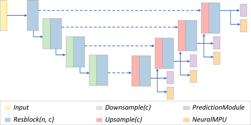
Figure 6. A U-Net built on our basic graph CNN operators. This network takes a dual octree graph with depth 6 as input, and predicts the octree splitting and corresponding volumetric fields.

Network

The overall network structure is shown in Fig. 6. We use $ResBlock(n,c)$ to represent a stack of $n$ ResNet blocks (He et al., 2016). Each ResNet block is constructed by concatenating two graph convolutions with a channel number of $c$. $Downsample(c)$ and $Upsample(c)$ are the graph downsampling and upsampling operators based on shared FC layers with the input and output channel as $c$. The extracted features at the end of each stage of the decoder are passed to a $PredictionModule$ to predict the octree splitting, which is made up of a shared MLP with 2 FC layers and 64 hidden units. Meanwhile, the extracted features are also passed to $NeuralMPU$ (defined in Section 3.3) to predict the field values. The U-Net shown in Fig. 6 takes a dual octree with depth 6 as input and output (resolution $64^{3}$), which is used for shape reconstruction in Section 4.1. When dealing with octrees with larger depth ($>6$), we add the required ResNet blocks and corresponding upsampling/downsampling operators accordingly based on the U-Net in Fig. 6. We set the maximum input/output octree depth as 7 (resolution $128^{3}$) in scene reconstruction in Section 4.3 and 8 (resolution $256^{3}$) in human body reconstruction in Section 4.4 for recovering the details of human hands and faces. Note that the output resolution of our method can be different from the input resolution because the MPU can generate features for any point in the 3D volume. The channel number $c$ is set as 196 when the octree depth is 3, 128 when 4, then decreases by a factor of 2 when the depth increases.

Octree Loss

When training the network to regress the ground-truth volumetric fields, we build an octree based on the ground-truth shapes as supervision. We use a binary cross entropy loss to train the network to determine whether the node is empty or not,

(5) $$\mathcal{L}_{octree}=\sum_{d}\frac{1}{N_{d}}\sum_{o\in\mathcal{O}_{d}}\operatorname{CrossEntropy}(o,o_{gt}),$$

where $d$ represents the depth of an octree layer, $N_{d}$ represents the total node number in the $d$-th layer, $O_{d}$ represents the predicted octree node status, and $o_{gt}$ is the corresponding ground-truth node status.

Regression Loss

To regress the ground-truth field values, we use the following $L_{2}$ loss:

(6) $$\mathcal{L}_{regress}=\sum_{d}\frac{1}{N_{\mathcal{P}}}\sum_{x\in\mathcal{P}}\left(\lambda_{v}\|F(x)-G(x)\|_{2}^{2}+\|\nabla F(x)-\nabla G(x)\|_{2}^{2}\right),$$

where $F(x)$ is the predicted volumetric fields, $G(x)$ is the ground-truth field values, and $\mathcal{P}$ is a set of query points. The gradient $\nabla G(x)$ is computed via finite difference, and $\nabla F(x)$ is computed by auto-differentiation. We set $\lambda_{v}$ as 200 to balance the two losses. The regression loss is also imposed on every layer of the octree, which we empirically find that it can slightly improve the final performance.

Gradient Loss

In surface reconstruction, the ground-truth field values are not known. We use the following gradient loss inspired by Posision surface reconstruction (Kazhdan et al., 2006):

(7) $$\begin{split}\mathcal{L}_{grad}=\sum_{d}\Big{\{}&\frac{1}{N_{\mathcal{S}}}\sum_{x\in\mathcal{S}}\left(\lambda_{v}\|F(x)\|_{2}^{2}+\|\nabla F(x)-\mathcal{N}(x)\|_{2}^{2}\right)+\\ &\frac{1}{N_{\mathcal{Q}}}\sum_{x\in\mathcal{Q}}\lambda_{g}\|\nabla F(x)\|_{2}^{2}\Big{\}},\end{split}$$

where $\mathcal{S}$ is a set of points from the input point cloud, $\mathcal{Q}$ is a set of points sampled uniformly from the 3D volume and $\mathcal{Q}\bigcap\mathcal{S}=\emptyset$, $\mathcal{N}(x)$ returns the normal of a point $x$ in $\mathcal{S}$, $\lambda_{v}$ and $\lambda_{g}$ is set to 200 and 0.1 respectively. $\mathcal{L}_{grad}$ encourages $F(x)=0,\nabla F(x)=\mathcal{N}(x),\forall x\in\mathcal{S}$ and $\nabla F(x)=0,\forall x\in\mathcal{Q}$, resulting in an occupancy field that approximates the input points and normals, and roughly equals $0.5$ outside the shape and $-0.5$ inside. Here, notice that the third term is different from the Eikonal loss used by IGR (Gropp et al., 2020), as the predicted volumeric field is an occupancy field, not an SDF field. We find that our occupancy field based loss function is not sensitive to network weight initialization, thus initializing our network randomly, while the SDF-field based loss design by IGR (Gropp et al., 2020) needs a special geometric initialization (Atzmon and Lipman, 2020).

4. Experiments and Discussions

We validate the efficiency and efficacy of our network on a series of 3D reconstruction tasks, including shape or scene reconstruction from noisy point clouds, unsupervised surface reconstruction, and autoencoders, and demonstrate its superiority to other state-of-the-art methods. All our experiments are conducted on 4 Nvidia V100 GPUs with 32GB memory.

4.1. Shape Reconstruction from Point Clouds

In this section, we train a network to reconstruct the volumetric representation of 3D shapes from noisy and sparse input point clouds. The ground-truth volumetric fields are needed during the training stage. Therefore, this task can also be regarded as a kind of shape super-resolution.

Dataset

We use man-made CAD shapes of 13 categories from ShapeNet to train the network and evaluate the performance following ConvONet (Peng et al., 2020), with the same data splitting. The original meshes of ShapeNet contain artifacts including flipped and overlapped triangles, self-intersections, and non-manifold geometry, we preprocess them to watertight meshes using the approach proposed in (Xu and Barbič, 2014) first, then normalize the meshes into a unit bounding box defined in $[-0.5,0.5]^{3}$ and compute the ground-truth SDF with the fast marching algorithm. To generate the input noisy point clouds, we randomly sample 3000 points for each mesh and add Gaussian noise with a standard deviation of 0.005, following the same sampling strategy as (Mescheder et al., 2019; Peng et al., 2020). For sampling the ground-truth SDF values to train the network, we first build octrees with depth 6 on watertight meshes, randomly sample 4 query points in each leaf node of the octree, and attach the corresponding SDF values to these points. This strategy resembles the sampling methods used in (Park et al., 2019; Liu et al., 2021), with which we can sample more points near the surface. These SDF samples are computed in the preprocessing step, and a subset is randomly drawn to evaluate the loss function in each training iteration.

Table 1. Quantitative evaluation on the ShapeNet dataset. The numbers outside and inside the parentheses are the results on the testing dataset of 13 categories from ShapeNet and on the 5 unseen categories respectively. The Chamfer distance (CD) is multiplied by a factor of 100 for better display.

Network	CD$\downarrow$	NC$\uparrow$	IoU$\uparrow$	F-Score$\uparrow$
ConvONet	0.438 (0.487)	0.932 (0.951)	0.852 (0.845)	0.925 (0.912)
DeepMLS	0.271 (0.302)	0.945 (0.957)	0.891 (0.894)	0.988 (0.985)
Ours	0.267 (0.286)	0.953 (0.967)	0.904 (0.918)	0.991 (0.990)

Evaluation Metrics

The output meshes are extracted with Marching Cubes (Lorensen and Cline, 1987) on a volumetric grid of $128^{3}$. Following ConvONet (Peng et al., 2020), we use the $L_{1}$ Chamfer distance (CD), normal consistency (NC), volumetric IoU, and F-Score as the evaluation metrics to measure the quality of the predicted meshes, among which the first two metrics measure the surface quality of the extracted meshes compared with ground-truth meshes and the last two metrics measure the volumetric quality of the output.

We denote the predicted mesh and ground-truth mesh by $M_{P}$ and $M_{G}$, on which we randomly sample a set of $N$ ($10k$) points $P=\{x_{i}\}_{i=1}^{N}$ and $G=\{y_{i}\}_{i=1}^{N}$, respectively. Define $\mathcal{P}_{A}(x)=\arg\min_{y\in A}\|x-y\|$, which finds the closest point of $x$ from a point set $A$. The $L_{1}$ Chamfer distance is defined as

(8) $$CD=\frac{1}{N}\sum_{i}\|x_{i}-\mathcal{P}_{G}(x_{i})\|+\frac{1}{N}\sum_{i}\|y_{i}-\mathcal{P}_{P}(y_{i})\|.$$

We define $\mathcal{N}(x)$ as an operator that returns the corresponding normal of an input point, then the normal consistency is defined as

(9) $$NC=\frac{1}{N}\sum_{i}|\mathcal{N}(x_{i})\cdot\mathcal{N}(\mathcal{P}_{G}(x_{i}))|+\frac{1}{N}\sum_{i}|\mathcal{N}(y_{i})\cdot\mathcal{N}(\mathcal{P}_{P}(y_{i}))|.$$

The volumetric IoU is defined as the volumetric intersection over union between $M_{P}$ and $M_{G}$, and we sample 100k points in the 3D volume to approximate the results. The F-Score is defined as the harmonic mean between the precision and the recall of points that lie within a certain distance between $M_{G}$ and $M_{P}$.

Implementation Details

We use Adam (Kingma and Ba, 2014) as the optimizer and train the network in 300 epochs with a batch size of 16. The initial learning rate is set as $10^{-3}$ and decreases to $10^{-5}$ linearly throughout the training process. The loss function is simply a summation of the octree loss (Eq. 5) and the regression loss (Eq. 6): $\mathcal{L}=\mathcal{L}_{octree}+\mathcal{L}_{regress}$. In each iteration, we randomly sample 5000 points from the ground-truth surface and 5000 points from the pre-computed SDF samples to evaluate the loss.

Results

We conduct a comparison with two recent learning-based methods that achieved top performance on this benchmark, including ConvONet (Peng et al., 2020), Deep Moving Least Squares (DeepMLS) (Liu et al., 2021) and the classical Poisson surface reconstruction (PSR) (Kazhdan et al., 2006). Our network has 2.2M parameters, which is between DeepMLS (4.6M) and ConvONet (1.1M). The numerical results are shown in Table 1, our method clearly achieves the best performance on all metrics. The visual comparisons are shown in Fig. 7. Since PSR needs point normals as input, we assign ground-truth normals to each point. It can be seen that the results of PSR are noisy and contain holes in the reconstructed shapes, even with ground-truth normals as additional input. The results of ConvONet are over-smoothed and lack fine geometric details. DeepMLS combines the octree-based U-Net (Wang et al., 2020) and moving least squares (Öztireli et al., 2009), and has higher expressiveness to reproduce the geometric details than ConvONet. However, DeepMLS also introduces high-frequency errors in the results, as shown in the back of the chair and the cells of the cabinet in Fig. 7. Moreover, DeepMLS constrains the output volumetric fields near the surface, the predicted representation of shapes is localized and the field values are undefined far away from the surface. Our network reconstructs the whole volumetric field made up of adaptive voxels: the low-resolution voxels help our network to fit the low-frequency part of the volumetric field, and the high-resolution voxels enable our network to reconstruct the fine geometric details. Therefore, our results are much more faithful to the ground-truth meshes visually and numerically.

Generalization Ability

To test the generalization ability of our network, we forward the networks on 5 unseen categories of ShapeNet, including bathtub, bag, bed, bottle, and pillow. We calculate the evaluation metrics and summarize the results in parentheses of Table 1. Our network achieves the highest performance on all metrics again. And the evaluation metrics do not change too much on these 5 unseen categories compared to the results on the testing dataset, which verifies that our network has strong generalization ability. The visual comparison is shown in the last row of Fig. 7, our network produces the best result and is significantly better than the others.

Table 2. Ablation study on the necessity of incorporating multiscale voxels in the convolution. O-CNN and SingleScale involve voxels of single scale in the convolution. Fine$\rightarrow$Coarse adds coarse voxels for fine-scale voxels when doing convolution. FullGraph operates on the full dual octree graph.

Network	CD$\downarrow$	NC$\uparrow$	IoU$\uparrow$	F-Score$\uparrow$
O-CNN	0.283	0.949	0.891	0.987
SingleScale	0.290	0.948	0.886	0.987
Fine$\rightarrow$Coarse	0.269	0.951	0.901	0.989
FullGraph	0.267	0.953	0.904	0.991

\begin{overpic}[width=424.94574pt]{shapenet} \put(2.0,-0.5){\small(a) Point cloud} \put(22.0,-0.5){\small(b) PSR} \put(36.0,-0.5){\small(c) ConvONet} \put(53.0,-0.5){\small(e) DeepMLS} \put(72.0,-0.5){\small(d) Ours} \put(86.0,-0.5){\small(e) Ground-truth} \end{overpic}

Figure 7. Shape-level reconstruction from noisy point clouds. The first three rows show the results from the testing dataset, and the last row shows the results of an unseen shape.

\begin{overpic}[width=416.27809pt]{ablation} \put(2.0,-0.5){\small(a) Point cloud} \put(18.0,-0.5){\small(b) {SingleScale}} \put(38.0,-0.5){\small(c) KPConv} \put(55.0,-0.5){\small(e) EdgeConv} \put(74.0,-0.5){\small(d) Ours} \put(88.0,-0.5){\small(e) Ground-truth} \end{overpic}

Figure 8. Visual comparison for different graph convolution designs.

4.2. Ablation Studies and Discussions

In this section, we study several key design choices and discuss the efficiency of our method on top of the experiment in Section 4.1.

Incorporate Multiscale Features in Convolutions

One of the key properties of our graph convolution is to keep all voxels covering the whole volume as active and involve multiscale voxel features in each convolution. To justify the necessity of this strategy, we design the following baselines.

• O-CNN: Use octree-based sparse convolution (O-CNN) (Wang et al., 2017) in the network. By combining O-CNN with our neural MPU, the network can also produce continuous volumetric fields. In this setting, only octree nodes with the same scale are involved in each convolution.

• SingleScale: Remove all cross-scale edges in the dual octree graph, which makes the graph convolution resemble O-CNN. The only difference is that the kernel shape of O-CNN is a cube with 27 neighborhoods, whereas the kernel shape of the graph convolution in this setting is a 3D cross with 7 neighborhoods. For a fair comparison, we reduce the channel size of O-CNN accordingly to ensure that the number of trainable parameters is similar.

• Fine$\rightarrow$Coarse: Based on SingleScale, add graph edges from fine-scale nodes to coarse-scale nodes so that fine octree nodes can exploit coarse-scale features during convolution.

We denote FullGraph as our default implementation that applies the graph convolution in the full dual octree. We use the same network settings and training configurations as in Section 4.1 and conduct experiments on ShapeNet. The results are summarized in Table 2. Based on the experiment results, we make the following observations:

• With a similar amount of trainable parameters, SingleScale is only slightly worse than O-CNN, even though the kernel size of SingleScale is smaller than O-CNN.

• By simply adding the edges from fine-scale to coarse-scale nodes, Fine$\rightarrow$Coarse is much better than SingleScale and O-CNN.

• By adding all edges to the dual octree graph, the performance of FullGraph improves further compared with Fine$\rightarrow$Coarse.

The visual comparison is shown in Fig. 8: the result of SingleScale contains unwanted holes compared with FullGraph. Given these observations, we draw the following conclusions:

• It is necessary to involve multiscale node features when performing convolutions. The coarse-scale features can help increase the receptive field and eliminate high-frequency errors.

• For cross-scale edges, the edges from coarse-scale nodes to fine-scale nodes are more critical for the final performance. We suspect that the fine-scale nodes have only a small volume coverage, thus being only slightly helpful for coarse-scale nodes.

Table 3. Performance comparisons among our graph convolution, KPConv and EdgeConv.

Network	CD$\downarrow$	NC$\uparrow$	IoU$\uparrow$	F-Score$\uparrow$	Train. Time$\downarrow$
KPConv	0.291	0.944	0.889	0.984	$89.1\text{\,}\mathrm{h}$
EdgeConv	0.289	0.945	0.891	0.982	$96.5\text{\,}\mathrm{h}$
Ours	0.267	0.953	0.904	0.991	$17.4\text{\,}\mathrm{h}$

\begin{overpic}[width=433.62pt]{scene} \put(5.0,0.0){\small(a) Point cloud} \put(28.0,0.0){\small(b) PSR} \put(46.0,0.0){\small(c) ConvONet} \put(68.0,0.0){\small(d) Ours} \put(86.0,0.0){\small(e) Ground-truth} \end{overpic}

Figure 9. Scene-level reconstruction from noisy point clouds. The results of PSR in column (b) are noisy and incomplete, and the results of ConvONet in column (c) lack fine geometric details and even miss reconstructing some objects in the scene, as highlighted in the zoom-in images.

Comparison with Other Point Convolutions

We compare our graph convolution tailored for dual octree graphs with previous widely-used point cloud convolutions, including EdgeConv (Wang et al., 2019) and KPConv (Thomas et al., 2019), to highlight the effectiveness and efficiency. In DGCNN (Wang et al., 2019), EdgeConv is originally applied to a dynamic KNN graph built in the feature space, we instead apply EdgeConv to our dual octree graph, otherwise, the network will be out-of-memory in runtime. We set the edge function of EdgeConv as an MLP with 2 hidden layers and 64 hidden units. For KPConv, we use its rigid version, which is similar to SplineConv (Fey et al., 2018). We set the radius of KPConv to the largest edge length of dual octree graphs. We also tried PointCNN (Li et al., 2018) and NNConv (Simonovsky and Komodakis, 2017), the training of the corresponding networks failed due to being out-of-memory.

We use the highly optimized implementations from the PyTorch Geometric library (Fey and Lenssen, 2019) to test these alterative graph convolution schemes. We use the same training configurations in Section 4.1. The evaluation metrics are summarized in Table 3. We also measure the total training time on 4 V100 GPUs, which are shown in the last column of Table 3. Our network not only achieves the best performance but also runs 5.1 times and 5.5 times faster than KPConv and EdgeConv respectively, justifying the benefits of taking into account the specific structure of the dual octree graph when designing the graph convolution. The visual comparisons shown in Fig. 8 also verify that with our graph convolution the network produces better results.

Benefits of Neural MPU

The neural MPU in Eq. 3 is used to guarantee the continuity of the resulting 3D field by interpolating features with different resolutions produced by our graph network. The trilinear interpolation used in ConvONet (Peng et al., 2020) can only deal with features defined on a 3D uniform grid. ACORN (Martel et al., 2021) can deal with adaptive features, whereas the resulting 3D fields are not continuous. The effect of our neural MPU can be verified by the extracted smooth iso-surfaces shown in Fig. 7.

Gradient Term in $\mathcal{L}_{regress}$

In $\mathcal{L}_{regress}$, we not only regress the ground-truth volumetric fields, but also add a gradient loss term following DeepMLS (Liu et al., 2021). We observe that the gradient loss is essential to improve the quality of the reconstructed 3D field. Without it, the performance of our method drops slightly (CD: 0.269, NC: 0.949, IoU: 0.901, F-Score: 0.990), but it still outperforms DeepMLS and ConvONet in Table 1.

Table 4. Time and GPU memory cost of our network, measured on a NVidia V100 GPU. The network takes a batch of 16 shapes for training and one single shape for inference, excluding marching cubes.

N	32	64	128	256
Training	6.1GB/174ms	10.7GB/271ms	16.8GB/489ms	27.2GB/924ms
Inference	0.4GB/41ms	0.7GB/55ms	1.1GB/91ms	1.5GB/153ms

Time and Memory Efficiency

The number of octree nodes increases quadratically with respect to volumetric resolution $N$, so our network has $\mathcal{O}(N^{2})$ memory and computational cost. We record the average memory and computational cost of our network with a batch of 16 shapes with a resolution of 64 for training and with one single shape for inference (excluding marching cubes) on a V100 GPU, and report the results in Table 4. As a reference, the memory footprints of the networks in Table 1 are $9.4\text{\,}\mathrm{G}\mathrm{B}$ for DeepMLS and $8.7\text{\,}\mathrm{G}\mathrm{B}$ for O-CNN with the same settings. ConvONet adopts a vanilla volumetric CNN, takes 7.5G memory with a resolution of 32, and runs out of memory with a resolution of 64 on the ShapeNet dataset. In summary, our network is as efficient as other octree-based networks, and much more efficient than volumetric CNNs.

\begin{overpic}[width=433.62pt]{dfaust} \put(2.0,-1.0){\small(a) Point Cloud} \put(18.0,-1.0){\small(b) IGR} \put(30.0,-1.0){\small(c) Ours} \put(39.0,-1.0){\small(d) Ground-truth} \put(53.0,-1.0){\small(e) Point Cloud} \put(68.0,-1.0){\small(f) IGR} \put(80.0,-1.0){\small(g) Ours} \put(89.0,-1.0){\small(h) Ground-truth} \end{overpic}

Figure 10. Visual results of surface reconstruction on D-Faust. IGR cannot reconstruct the hands of the body shapes, as highlighted by the red box. IGR produces fake surface sheets on the feet.

4.3. Scene Reconstruction from Point Clouds

In this section, we conduct experiments on scene-level datasets to verify the scalability of our method. The network takes a noisy point cloud sampled from scene-level data as input and regresses the corresponding volumetric occupancy fields.

Dataset

We use the synthetic scene dataset provided by ConvONet (Peng et al., 2020). The dataset contains $5k$ scenes with randomly selected objects from 5 categories of ShapeNet, including chair, sofa, lamp, cabinet, and table. Following ConvONet, we uniformly sample $10k$ points from each scene, add Gaussian noise with a standard deviation of 0.05 as input, and let the network regress the ground-truth occupancy values. We also use the same data splitting as ConvONet. We set the octree depth as 7, and the equivalent maximum voxel resolution is $128^{3}$.

Training Details

We use Adam (Kingma and Ba, 2014) as the optimizer with a batch size of 16. The initial learning rate is set as $10^{-3}$ and decreases to $10^{-5}$ linearly throughout the training process. We trained the network in 900 epochs, with the similar training iteration number as ConvONet. The loss function is defined as $\mathcal{L}=\mathcal{L}_{octree}+\mathcal{L}_{regress}$. In each iteration, we randomly sample 10000 points from the ground-truth surfaces and 10000 points from ground-truth occupancy values in the 3D volume to evaluate the loss.

Results

We compare our method with ConvONet (Peng et al., 2020), ONet (Mescheder et al., 2019) and PSR (Kazhdan et al., 2006). We calculate the metrics defined in Section 4.1, and the results are shown in Table 5. For ConvONet, we use the code released by the authors to generate the results. For ONet, we directly reuse the results provided by (Peng et al., 2020). Our method is consistently better than the other methods. ConvONet uses dense voxels with resolution $64^{3}$ in the network. However, due to the constraints of computation and memory caused by dense voxels, the CNN layers operating on higher resolution features are shallow and have low expressiveness. Our network directly outputs adaptive volumetric grids with the finest resolution up to $128^{3}$, and our network has a stack of CNN blocks even on high-resolution features, so our network can reconstruct fine details faithfully. We also record the running time of network forwarding and field evaluation on $128^{3}$ uniformly sampled query points in the testing stage, excluding the time of marching cubes and hard disk I/O. Table 5 shows our network is 2.7 times faster than ConvONet in performing this task.

The visual results are shown in Fig. 9, it is obvious that our results are more faithful to the ground-truth meshes. The results of PSR are noisy and incomplete due to the lack of priors from the dataset. ConvONet cannot reproduce fine details and may also fail to reconstruct some objects in the scene, as highlighted in Fig. 9.

Table 5. Quantitative evaluation on the scene-level dataset. The results of ONet are provided by ConvONet.

Network	CD$\downarrow$	NC$\uparrow$	IoU$\uparrow$	F-Score$\uparrow$	Time$\downarrow$
ONet	2.100	0.783	0.475	-	-
ConvONet	0.419	0.914	0.849	0.964	0.857s
Ours	0.388	0.923	0.857	0.969	0.314s

\begin{overpic}[width=433.62pt]{recons} \end{overpic}

Figure 11. Surface reconstruction on shapes with rich geometric details. The network trained on D-Faust directly takes a point cloud as input and predicts the corresponding volumetric field by a single forward pass.

4.4. Unsupervised Surface Reconstruction

In this section, we focus on surface reconstruction from raw point clouds. Surface reconstruction is a fundamental problem in computer graphics and has drawn much attention over the past few decades (Berger et al., 2017). In surface reconstruction, ground-truth volumetric field values are unknown or impossible to compute in advance, therefore the network is trained without the supervision of ground-truth volumetric field values.

Dataset

We use the D-Faust dataset (Bogo et al., 2017) following IGR (Gropp et al., 2020). D-Faust contains real scans of human bodies in different poses, in which $6k$ scans are used for training and $2k$ scans for testing. We use the raw point clouds with normals as input and set the octree depth to 8, with an equivalent volumetric resolution of $256^{3}$. The point clouds are incomplete and noisy, caused by occlusion in the scanning process and limited precision of scanners.

Training details

The training settings are the same as Section 4.3, except that we set the maximal training epoch to 600. Since there are no ground-truth field values, we trained the network with $\mathcal{L}_{grad}$ in Eq. 7. The octrees in the encoder and decoder are the same, therefore we do not use the octree loss $\mathcal{L}_{octree}$. In each training iteration, we randomly sample 10k points from the point cloud and the 3D volume for each shape to evaluate the loss function.

Table 6. Quantitative evaluation on D-Faust. CD(pred, gt) is the one-side chamfer distance from the predicted meshes to the ground-truth meshes, and vice versa for CD(gt, pred).

Network	CD$\downarrow$	NC$\uparrow$	CD(pred, gt)$\downarrow$	CD(gt, pred) $\downarrow$	Time$\downarrow$
IGR	0.499	0.875	0.854	0.143	110.8s
Ours	0.048	0.964	0.048	0.047	0.281s

Results

We conduct the comparison with IGR (Gropp et al., 2020) using the code provided by the authors. In SALD (Atzmon and Lipman, 2021), IGR has already been thoroughly compared with SAL (Atzmon and Lipman, 2020) and SALD on D-Faust: SAL cannot reconstruct geometry details compared with IGR, and SALD achieves a similar numerical performance to IGR. The key difference between IGR and SAL/SALD is the loss function. The recently proposed ACORN (Martel et al., 2021) requires the ground-truth volumetric field values as the training target and cannot be used in this task, as the volumetric fields of ACORN are not continuous and the gradient is not well defined. Thus, we mainly conduct the comparison with IGR, and the results are summarized in Table 6. For evaluation, we report the Chamfer distance and normal consistency in Section 4.1, as well as the one-side Chamfer distance following IGR. Since the output meshes of IGR are often incomplete as shown in Fig. 10, the mIoU for IGR is not well defined, thus we omit this metric in this experiment. According to Table 6, our results are clearly much better than IGR. Especially, the Chamfer distance of our results is smaller than that of IGR by one order. The visual comparisons in Fig. 10 demonstrate that IGR has a poor ability to reconstruct geometric details from input point clouds, for example, the hands of the bodies are missing, as highlighted in the red box. Additionally, the reconstructed shapes of IGR contain fake surface sheets on the feet, as shown in Fig. 10.

We need to mention that IGR is based on the autodecoder proposed by (Park et al., 2019). For each testing shape, the latent code has to be optimized separately by 800 iterations according to the setting of IGR, therefore IGR consumes a lot of time in the testing stage. Our network can produce the output directly in a single forward pass. We also record the average running time of producing one result from the testing dataset in Table 6. Our method runs extremely fast and is 394 times faster than IGR on average.

Generalization Ability

We observe that our network trained on D-Faust demonstrates strong generalization ability. We directly apply the trained network to several point clouds from the Stanford 3D Scanning Repository and 2 scene-level point clouds from SceneNN (Handa et al., 2016). The results of surface reconstruction are shown in Fig. 11 and Fig. 1. Previous state-of-the-art learning-based surface reconstruction methods, like SIREN (Sitzmann et al., 2020), need several hours to train the network to get similar results, while our network generates these results by a single forward pass, which takes about $420\text{\,}\mathrm{m}\mathrm{s}$ on average for the meshes in Fig. 11.

\begin{overpic}[width=433.62pt]{lucy} \put(4.0,-3.0){\small(a) Initial output} \put(38.0,-3.0){\small(b) After fintuning} \put(72.0,-3.0){\small(c) Ground-truth} \end{overpic}

Figure 12. Improve the surface reconstruction with finetuning. (a) is the initial output of our pretrained network, (b) is the improved output after 2000 iterations of finetuning. The details near the mouth of Lucy are gradually recovered.

Finetuning

Given the pretrained weights, we can finetune the network to further improve the results. In Fig. 12, we finetuned the network with the same loss function by 2000 iterations with Adam and a learning rate of 0.0001. More geometric features are reproduced gradually after finetuning.

4.5. Autoencoder

In the previous sections, we conduct experiments with U-Net. In this section, we further verify the flexibility and effectiveness of our method with an autoencoder, which does not have skip connections between the encoder and the decoder.

Dataset

We train an autoencoder with 13 categories of CAD shapes from ShapeNet (Chang et al., 2015) and used the same data splitting as IM-Net (Chen and Zhang, 2019): 35019 shapes for training and 8762 shapes for testing. The data preprocessing is the same as Section 4.1, and the depth of the octree is set as 6.

\begin{overpic}[width=433.62pt]{ae} \put(13.0,-2.0){\small(a) IM-Net} \put(49.0,-2.0){\small(b) Ours} \put(74.0,-2.0){\small(c) Ground-truth} \end{overpic}

Figure 13. Visual results of autoencoders. The results of IM-Net have artifacts and contain less details as highlighted in the red boxes.

Table 7. Quantitative evaluation of autoencoders on ShapeNet. The Chamfer distance (CD) is multiplied by 100 for better display.

Network	CD$\downarrow$	NC$\uparrow$	Time$\downarrow$
AtlasNet	1.17	0.807	-
OccNet	1.94	0.821	-
IM-Net	1.37	0.811	0.841s
Ours	0.89	0.921	0.143s

Results

We use the same training settings and loss function as Section 4.1. We report the evaluation metrics in Table 7. The results of AtlasNet (Groueix et al., 2018) and OccNet (Mescheder et al., 2019) are provided by the authors of IM-Net (Chen and Zhang, 2019), and we use the code of IM-Net to generate its results. In this experiment, the Chamfer distance and normal consistency are calculated with 4096 sample points following IM-Net. The encoders of both IM-Net and OccNet are a volumetric CNN, and their decoders are a coordinate-based MLP. The network of AtlasNet is a point-based autoencoder. And all networks are trained on 13 categories. It is clear that our performance is significantly better than IM-Net, OccNet, and AtlasNet. The results further verify the effectiveness of our network over coordinate-based MLPs in learning volumetric fields. For running time, we record the average time of a network forward pass and query the field values of $100^{3}$ uniformly sampled points for each shape in the testing dataset. As shown in the last column of Table 7, our method is 5.9 times faster than IM-Net. The visual comparison is shown in Fig. 13. Compared with IM-Net, our results are more similar to ground truth, while IM-Net cannot faithfully reconstruct the base of the chair and engine of the airplane.

5. Conclusion

In this paper, we propose dual octree-based graph neural networks to learn adaptive volumetric shape representations. We use an octree to partition the 3D volume into adaptive voxels and build a dual graph to connect adjacent voxels. We propose a novel graph convolution, which operates on voxels with multiple resolutions, and construct encoder and decoder networks to extract adaptive features. We blend these features with a novel neural MPU module to generate continuous volumetric fields. Our method demonstrates great efficiency and achieves state-of-the-art performance in a series of shape reconstruction tasks.

In our work, the following aspects are not fully investigated, and we would like to explore them further.

Concurrent Downsampling and Upsampling on Leaf Nodes

In our current implementation, at one time, only the octree nodes at one level are merged during graph downsampling, or subdivided during graph upsampling. Another possible strategy is to run these operators on all leaf nodes in different levels simultaneously, so that the messages between nodes can be passed and aggregated via the adaptive hierarchy of the dual octree more effectively. We would like to explore whether this alternative strategy can further maximize the performance of our network.

Optimal Octree Structure

Currently, the adaptiveness of the feature volume in the encoder and decoder is determined by the pre-built octree based on the input, which may not be optimal. It is possible to combine the octree optimization procedure proposed in ACORN (Martel et al., 2021) with our network to increase the compactness of the octree and further improve efficiency.

Shape Analysis

Our graph convolution is general and can also be used in shape analysis. We have built a ResNet with our graph convolution and tested it on the ModelNet40 classification (Wu et al., 2015). The classification accuracy is promising: 92.4%, although it does not outperform other state-of-the-art networks, such as DGCNN (Wang et al., 2019) (92.9%) or PCT (Guo et al., 2021) (93.2%). In the future, we would like to explore more possibilities for applying our method to shape analysis, especially for shapes in volumetric representations.

- (1)
- Atzmon and Lipman (2020) Matan Atzmon and Yaron Lipman. 2020. SAL: Sign agnostic learning of shapes from raw data. In CVPR.
- Atzmon and Lipman (2021) Matan Atzmon and Yaron Lipman. 2021. SALD: Sign Agnostic Learning with Derivatives. In ICLR.
- Battaglia et al. (2018) Peter W Battaglia, Jessica B Hamrick, Victor Bapst, Alvaro Sanchez-Gonzalez, Vinicius Zambaldi, Mateusz Malinowski, Andrea Tacchetti, David Raposo, Adam Santoro, Ryan Faulkner, et al. 2018. Relational inductive biases, deep learning, and graph networks. arXiv preprint arXiv:1806.01261 (2018).
- Berger et al. (2017) Matthew Berger, Andrea Tagliasacchi, Lee M. Seversky, Pierre Alliez, Gaël Guennebaud, Joshua A. Levine, Andrei Sharf, and Claudio T. Silva. 2017. A survey of surface reconstruction from point clouds. Comput. Graph. Forum 36, 1 (2017).
- Bogo et al. (2017) Federica Bogo, Javier Romero, Gerard Pons-Moll, and Michael J Black. 2017. Dynamic FAUST: Registering human bodies in motion. In CVPR.
- Bridson (2015) Robert Bridson. 2015. Fluid simulation for computer graphics. CRC press.
- Brock et al. (2016) Andrew Brock, Theodore Lim, J.M. Ritchie, and Nick Weston. 2016. Generative and discriminative voxel modeling with convolutional neural networks. In 3D deep learning workshop (NeurIPS).
- Chabra et al. (2020) Rohan Chabra, Jan Eric Lenssen, Eddy Ilg, Tanner Schmidt, Julian Straub, Steven Lovegrove, and Richard Newcombe. 2020. Deep Local Shapes: Learning Local SDF Priors for Detailed 3D Reconstruction. In ECCV.
- Chang et al. (2015) Angel X. Chang, Thomas Funkhouser, Leonidas Guibas, Pat Hanrahan, Qixing Huang, Zimo Li, Silvio Savarese, Manolis Savva, Shuran Song, Hao Su, Jianxiong Xiao, Li Yi, and Fisher Yu. 2015. ShapeNet: An information-rich 3D model repository. arXiv preprint arXiv:1512.03012 (2015).
- Chen and Zhang (2019) Zhiqin Chen and Hao Zhang. 2019. Learning implicit fields for generative shape modeling. In CVPR.
- Chibane et al. (2020) Julian Chibane, Thiemo Alldieck, and Gerard Pons-Moll. 2020. Implicit functions in feature space for 3d shape reconstruction and completion. In CVPR.
- Choy et al. (2019) Christopher Choy, JunYoung Gwak, and Silvio Savarese. 2019. 4D spatio-temporal convnets: Minkowski convolutional neural networks. In CVPR.
- Choy et al. (2016) Christopher Choy, Danfei Xu, JunYoung Gwak, Kevin Chen, and Silvio Savarese. 2016. 3D-R2N2: A unified approach for single and multi-view 3D object reconstruction. In ECCV.
- Curless and Levoy (1996) Brian Curless and Marc Levoy. 1996. A Volumetric Method for Building Complex Models from Range Images. In SIGGRAPH.
- Dai et al. (2017) Angela Dai, Charles R. Qi, and Matthias Niessner. 2017. Shape completion using 3D-encoder-predictor CNNs and shape synthesis. In CVPR.
- Fey and Lenssen (2019) Matthias Fey and Jan Eric Lenssen. 2019. Fast Graph Representation Learning with PyTorch Geometric. In ICLR Workshop.
- Fey et al. (2018) Matthias Fey, Jan Eric Lenssen, Frank Weichert, and Heinrich Müller. 2018. SplineCNN: Fast Geometric Deep Learning with Continuous B-Spline Kernels. In CVPR.
- Genova et al. (2020) Kyle Genova, Forrester Cole, Avneesh Sud, Aaron Sarna, and Thomas Funkhouser. 2020. Local Deep Implicit Functions for 3D Shape. In CVPR.
- Gilmer et al. (2017) Justin Gilmer, Samuel S Schoenholz, Patrick F Riley, Oriol Vinyals, and George E Dahl. 2017. Neural message passing for quantum chemistry. In ICML.
- Graham et al. (2018) Benjamin Graham, Martin Engelcke, and Laurens van der Maaten. 2018. 3D semantic segmentation with submanifold sparse convolutional networks. In CVPR.
- Gropp et al. (2020) Amos Gropp, Lior Yariv, Niv Haim, Matan Atzmon, and Yaron Lipman. 2020. Implicit geometric regularization for learning shapes. In ICML.
- Groueix et al. (2018) Thibault Groueix, Matthew Fisher, Vladimir G. Kim, Bryan C. Russell, and Mathieu Aubry. 2018. AtlasNet: A Papier-Mâché approach to learning 3D surface generation. In CVPR.
- Guo et al. (2021) Meng-Hao Guo, Jun-Xiong Cai, Zheng-Ning Liu, Tai-Jiang Mu, Ralph R Martin, and Shi-Min Hu. 2021. PCT: Point cloud transformer. Computational Visual Media 7, 2 (2021).
- Handa et al. (2016) Ankur Handa, Viorica Patraucean, Vijay Badrinarayanan, Simon Stent, and Roberto Cipolla. 2016. SceneNet: Understanding Real World Indoor Scenes With Synthetic Data. In CVPR.
- Häne et al. (2017) Christian Häne, Shubham Tulsiani, and Jitendra Malik. 2017. Hierarchical surface prediction for 3D object reconstruction. In 3DV.
- He et al. (2016) Kaiming He, Xiangyu Zhang, Shaoqing Ren, and Jian Sun. 2016. Deep residual learning for image recognition. In CVPR.
- Jiang et al. (2020) Chiyu Jiang, Avneesh Sud, Ameesh Makadia, Jingwei Huang, Matthias Nießner, and Thomas Funkhouser. 2020. Local implicit grid representations for 3D scenes. In CVPR.
- Ju et al. (2002) Tao Ju, Frank Losasso, Scott Schaefer, and Joe Warren. 2002. Dual contouring of hermite data. ACM Trans. Graph. (SIGGRAPH) (2002).
- Kazhdan et al. (2006) Michael Kazhdan, Matthew Bolitho, and Hugues Hoppe. 2006. Poisson surface reconstruction. In Symp. Geom. Proc.
- Kingma and Ba (2014) Diederik P. Kingma and Jimmy Ba. 2014. Adam: A method for stochastic optimization. In ICLR.
- León et al. (2008) Alejandro León, Juan Carlos Torres, and Francisco Velasco. 2008. Volume octree with an implicitly defined dual grid. Computers & Graphics 32, 4 (2008).
- Lewiner et al. (2010) Thomas Lewiner, Vinícius Mello, Adelailson Peixoto, Sinésio Pesco, and Hélio Lopes. 2010. Fast Generation of Pointerless Octree Duals. Computer Graphics Forum 29, 5 (2010).
- Li et al. (2018) Yangyan Li, Rui Bu, Mingchao Sun, Wei Wu, Xinhan Di, and Baoquan Chen. 2018. PointCNN: Convolution on X-transformed points. In NeurIPS.
- Liu et al. (2021) Shi-Lin Liu, Hao-Xiang Guo, Hao Pan, Peng-Shuai Wang, Xin Tong, and Yang Liu. 2021. Deep Implicit Moving Least-Squares Functions for 3D Reconstruction. In CVPR.
- Lorensen and Cline (1987) William E. Lorensen and Harvey E. Cline. 1987. Marching Cubes: A High Resolution 3D Surface Construction Algorithm. In SIGGRAPH.
- Martel et al. (2021) Julien N. P. Martel, David B. Lindell, Connor Z. Lin, Eric R. Chan, Marco Monteiro, and Gordon Wetzstein. 2021. ACORN: Adaptive coordinate networks for neural scene representation. ACM Trans. Graph. (SIGGRAPH) 40, 4 (2021).
- Maturana and Scherer (2015) Daniel Maturana and Sebastian Scherer. 2015. VoxNet: A 3D convolutional neural network for real-time object recognition. In IROS.
- Mescheder et al. (2019) Lars Mescheder, Michael Oechsle, Michael Niemeyer, Sebastian Nowozin, and Andreas Geiger. 2019. Occupancy networks: Learning 3D reconstruction in function space. In CVPR.
- Mildenhall et al. (2020) Ben Mildenhall, Pratul P Srinivasan, Matthew Tancik, Jonathan T Barron, Ravi Ramamoorthi, and Ren Ng. 2020. NeRF: Representing scenes as neural radiance fields for view synthesis. In ECCV.
- Müller et al. (2022) Thomas Müller, Alex Evans, Christoph Schied, and Alexander Keller. 2022. Instant Neural Graphics Primitives with a Multiresolution Hash Encoding. arXiv preprint arXiv:2201.05989 (2022).
- Oechsle et al. (2019) Michael Oechsle, Lars Mescheder, Michael Niemeyer, Thilo Strauss, and Andreas Geiger. 2019. Texture fields: Learning texture representations in function space. In ICCV.
- Ohtake et al. (2003) Yutaka Ohtake, Alexander Belyaev, Marc Alexa, Greg Turk, and Hans-Peter Seidel. 2003. Multi-level partition of unity implicits. ACM Trans. Graph. (SIGGRAPH) 22, 3 (2003).
- Öztireli et al. (2009) A Cengiz Öztireli, Gael Guennebaud, and Markus Gross. 2009. Feature preserving point set surfaces based on non-linear kernel regression. Comput. Graph. Forum (EG) 28, 2 (2009).
- Park et al. (2019) Jeong Joon Park, Peter Florence, Julian Straub, Richard Newcombe, and Steven Lovegrove. 2019. DeepSDF: Learning continuous signed distance functions for shape representation. In CVPR.
- Peng et al. (2020) Songyou Peng, Michael Niemeyer, Lars Mescheder, Marc Pollefeys, and Andreas Geiger. 2020. Convolutional occupancy networks. In ECCV.
- Qi et al. (2017a) Charles R. Qi, Hao Su, Kaichun Mo, and Leonidas J. Guibas. 2017a. PointNet: Deep learning on point sets for 3D classification and segmentation. In CVPR.
- Qi et al. (2016) Charles R. Qi, Hao Su, Matthias Nießner, Angela Dai, Mengyuan Yan, and Leonidas J. Guibas. 2016. Volumetric and multi-view CNNs for object classification on 3D data. In CVPR.
- Qi et al. (2017b) Charles R. Qi, Li Yi, Hao Su, and Leonidas J. Guibas. 2017b. PointNet++: Deep hierarchical feature learning on point sets in a metric space. In NeurIPS.
- Ronneberger et al. (2015) Olaf Ronneberger, Philipp Fischer, and Thomas Brox. 2015. U-Net: Convolutional networks for biomedical image segmentation. In International Conference on Medical image computing and computer-assisted intervention.
- Schaefer and Warren (2004) Scott Schaefer and Joe Warren. 2004. Dual marching cubes: Primal contouring of dual grids. In Pacific Graphics.
- Shao et al. (2018) Tianjia Shao, Yin Yang, Yanlin Weng, Qiming Hou, and Kun Zhou. 2018. H-CNN: spatial hashing based CNN for 3D shape analysis. IEEE. T. Vis. Comput. Gr. (2018).
- Sharf et al. (2007) Andrei Sharf, Thomas Lewiner, Gil Shklarski, Sivan Toledo, and Daniel Cohen-Or. 2007. Interactive topology-aware surface reconstruction. ACM Trans. Graph. (SIGGRAPH) 26, 3 (2007).
- Simonovsky and Komodakis (2017) Martin Simonovsky and Nikos Komodakis. 2017. Dynamic edge-conditioned filters in convolutional neural networks on graphs. In CVPR.
- Sitzmann et al. (2020) Vincent Sitzmann, Julien NP Martel, Alexander W Bergman, David B Lindell, and Gordon Wetzstein. 2020. Implicit Neural Representations with Periodic Activation Functions. In NeurIPS.
- Takikawa et al. (2021) Towaki Takikawa, Joey Litalien, Kangxue Yin, Karsten Kreis, Charles Loop, Derek Nowrouzezahrai, Alec Jacobson, Morgan McGuire, and Sanja Fidler. 2021. Neural Geometric Level of Detail: Real-time Rendering with Implicit 3D Shapes. In CVPR.
- Tancik et al. (2020) Matthew Tancik, Pratul P. Srinivasan, Ben Mildenhall, Sara Fridovich-Keil, Nithin Raghavan, Utkarsh Singhal, Ravi Ramamoorthi, Jonathan T. Barron, and Ren Ng. 2020. Fourier Features Let Networks Learn High Frequency Functions in Low Dimensional Domains. In NeurIPS.
- Tang et al. (2021) Jia-Heng Tang, Weikai Chen, Jie Yang, Bo Wang, Songrun Liu, Bo Yang, and Lin Gao. 2021. OctField: Hierarchical Implicit Functions for 3D Modeling. In NeurIPS.
- Tatarchenko et al. (2017) Maxim Tatarchenko, Alexey Dosovitskiy, and Thomas Brox. 2017. Octree generating networks: efficient convolutional architectures for high-resolution 3D outputs. In ICCV.
- Thomas et al. (2019) Hugues Thomas, Charles R. Qi, Jean-Emmanuel Deschaud, Beatriz Marcotegui, François Goulette, and Leonidas J. Guibas. 2019. KPConv: Flexible and deformable convolution for point clouds. In ICCV.
- Ummenhofer and Koltun (2021) Benjamin Ummenhofer and Vladlen Koltun. 2021. Adaptive Surface Reconstruction With Multiscale Convolutional Kernels. In ICCV.
- Veličković et al. (2018) Petar Veličković, Guillem Cucurull, Arantxa Casanova, Adriana Romero, Pietro Liò, and Yoshua Bengio. 2018. Graph Attention Networks. In ICLR.
- Wang et al. (2018a) Hao Wang, Nadav Schor, Ruizhen Hu, Haibin Huang, Daniel Cohen-Or, and Hui Huang. 2018a. Global-to-local generative model for 3D shapes. ACM Trans. Graph. (SIGGRAPH ASIA) 37, 6 (2018).
- Wang et al. (2017) Peng-Shuai Wang, Yang Liu, Yu-Xiao Guo, Chun-Yu Sun, and Xin Tong. 2017. O-CNN: Octree-based convolutional neural networks for 3D shape analysis. ACM Trans. Graph. (SIGGRAPH) 36, 4 (2017).
- Wang et al. (2020) Peng-Shuai Wang, Yang Liu, and Xin Tong. 2020. Deep Octree-based CNNs with Output-Guided Skip Connections for 3D Shape and Scene Completion. In CVPR Workshop.
- Wang et al. (2018b) Peng-Shuai Wang, Chun-Yu Sun, Yang Liu, and Xin Tong. 2018b. Adaptive O-CNN: A patch-based deep representation of 3D shapes. ACM Trans. Graph. (SIGGRAPH ASIA) 37, 6 (2018).
- Wang et al. (2019) Yue Wang, Yongbin Sun, Ziwei Liu, Sanjay E Sarma, Michael M Bronstein, and Justin M Solomon. 2019. Dynamic graph CNN for learning on point clouds. ACM Trans. Graph. 38, 5 (2019).
- Williams et al. (2022) Francis Williams, Zan Gojcic, Sameh Khamis, Denis Zorin, Joan Bruna, Sanja Fidler, and Or Litany. 2022. Neural Fields as Learnable Kernels for 3D Reconstruction. In CVPR.
- Williams et al. (2021) Francis Williams, Matthew Trager, Joan Bruna, and Denis Zorin. 2021. Neural splines: Fitting 3D surfaces with infinitely-wide neural networks. In CVPR.
- Wu et al. (2016) Jiajun Wu, Chengkai Zhang, Tianfan Xue, William T. Freeman, and Joshua B. Tenenbaum. 2016. Learning a probabilistic latent space of object shapes via 3D generative-adversarial modeling. In NeurIPS.
- Wu et al. (2019) Wenxuan Wu, Zhongang Qi, and Li Fuxin. 2019. PointConv: Deep Convolutional Networks on 3D Point Clouds. In CVPR.
- Wu et al. (2020) Zonghan Wu, Shirui Pan, Fengwen Chen, Guodong Long, Chengqi Zhang, and S Yu Philip. 2020. A comprehensive survey on graph neural networks. IEEE Transactions on Neural Networks and Learning Systems 32, 1 (2020).
- Wu et al. (2015) Zhirong Wu, Shuran Song, Aditya Khosla, Fisher Yu, Linguang Zhang, Xiaoou Tang, and Jianxiong Xiao. 2015. 3D ShapeNets: A deep representation for volumetric shape modeling. In CVPR.
- Xu and Barbič (2014) Hongyi Xu and Jernej Barbič. 2014. Signed Distance Fields for Polygon Soup Meshes. In Proceedings of Graphics Interface.
- Xu et al. (2021) Mutian Xu, Runyu Ding, Hengshuang Zhao, and Xiaojuan Qi. 2021. PAConv: Position Adaptive Convolution with Dynamic Kernel Assembling on Point Clouds. In CVPR.
- Xu et al. (2018) Yifan Xu, Tianqi Fan, Mingye Xu, Long Zeng, and Yu Qiao. 2018. SpiderCNN: Deep Learning on Point Sets with Parameterized Convolutional Filters. In ECCV.
- Zhao et al. (2021) Hengshuang Zhao, Li Jiang, Jiaya Jia, Philip Torr, and Vladlen Koltun. 2021. Point transformer. In ICCV.
- Zhou et al. (2011) Kun Zhou, Minmin Gong, Xin Huang, and Baining Guo. 2011. Data-parallel octrees for surface reconstruction. IEEE. T. Vis. Comput. Gr. 17, 5 (2011).