Influence of chirp and carrier-envelope phase on non-integer high-harmonic generation

Abstract

High harmonic generation (HHG) is a versatile technique for probing ultrafast electron dynamics. While HHG is sensitive to the electronic properties of the target, HHG also depends on the waveform of the laser pulse. As is well known, (peak) positions, $\omega$, in the high-harmonic spectrum can shift when the carrier envelope phase (CEP), $\varphi$ is varied. We derive formulæ describing the corresponding parametric dependencies of CEP shifts; in particular, we have a transparent result for the (peak) shift, $d\omega/d\varphi\hskip 1.69998pt{=}\hskip 1.69998pt{-}\hskip 0.50003pt2\hskip 0.50003pt\bar{\mathfrak{f}}^{\prime}\omega/\omega_{0}$, where $\omega_{0}$ describes the fundamental frequency and $\bar{\mathfrak{f}}^{\prime}$ characterizes the chirp of the driving laser pulse. We compare the analytical formula to full-fledged numerical simulations finding only 17 % average relative absolute deviation in $d\omega/d\varphi$. Our analytical result is fully consistent with experimental observations.

I Introduction

High harmonic generation (HHG) is a unique fingerprint of ultrafast electron dynamics in solids: [1, 2, 3, 4, 5, 6, 7, 8, 9, 10, 11, 12, 13, 14, 15, 16, 17, 18, 19, 20, 21, 22, 23, 24, 25, 26, 27] It is generated when atomically strong electric fields drive charge currents that in turn emit electromagnetic radiation. In solids, such currents are understood as interband transitions and (semiclassical) intraband currents. The emitted light supports frequencies much higher than those of the driving field, see also Fig. 1 as an illustration. Since high harmonics are sensing acceleration processes of the charge carriers, HHG can be used for monitoring dynamical processes. The information thus incorporated allows to reconstruct band structures; [14, 15] it reflects dynamical Bloch oscillations [3, 6, 28] and Berry phase effects. [18, 19, 20, 29, 30, 31, 32, 33, 21, 22, 34, 35, 36]

In the past, HHG has been analyzed to study charge carrier dynamics in dielectrics [2, 6, 11, 13] and semiconductors. [3, 4, 5] Fresh applications to three-dimensional topological insulators and their gapless surface states have been published recently. [10, 37] These surface states have been argued to be an ideal platform for lightwave electronics. [38, 10] This is because the suppression of backscattering due to the spin-momentum locking makes it easier to facilitate quantum control for long times. [39, 38, 10]

An intriguing feature of topological surface states is the effect of the carrier-envelope phase (CEP) [40, 41, 42, 43, 44, 45, 46] on the high-harmonic spectrum: upon tuning the CEP, harmonic orders shift continuously to non-integer multiples of the driving frequency $\omega_{0}$. [10] This is illustrated in Fig. 1, where we display the HHG for a topological surface state; for the two CEP-values shown, the peaks of orders 13-18 are shifted against each other by $\omega_{0}/2$. Corresponding shifts have been observed before in semiconductors [3, 23, 24] and dielectrics [11, 13, 25, 26]; the particular aspect of topological surfaces is that CEP shifts occur at relatively low harmonic order [10].

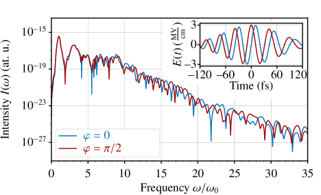
Figure 1: High-harmonic emission spectrum $I(\omega)$ as function of the frequency $\omega$ computed from semiconductor Bloch equations (SBE), [47, 48, 49, 50, 51, 52, 53, 54, 55, 56, 57, 58, 59, 16] Eq. (5). For the SBE simulation, we employ a two-band Hamiltonian [10] to model the topological surface state of Bi₂Te₃. As driving electric field ${\bf E}(t)$ (inset), we use Eq. (4) with $E_{0}\hskip 1.52998pt{=}\hskip 1.52998pt3\,$MV/cm, $\omega_{0}\hskip 1.52998pt{=}\hskip 1.52998pt2\pi\hskip 1.52998pt{\cdot}\hskip 1.52998pt25$ THz, $f_{\text{chirp}}\hskip 1.52998pt{=}\hskip 1.52998pt-$1.25 THz, $\sigma\hskip 1.52998pt{=}\hskip 1.52998pt90$ fs as used in simulations in Ref. 10. We employ two different CEPs, $\varphi\hskip 1.52998pt{=}\hskip 1.52998pt0$ (blue) and $\varphi\hskip 1.52998pt{=}\hskip 1.52998pt\pi/2$ (red). The driving electric field $E(t)$ is sketched in the inset.

In this work, we develop a minimal model of high harmonic generation that explains the CEP shifts in analytical terms. The main result of our work is that under a tuning of the CEP by $d\varphi$, the frequency $\omega$ of high harmonics shifts by

$$d\omega=-\,2\,\frac{\omega}{\omega_{0}}\,\bar{\mathfrak{f}}^{\prime}\,d\varphi\,;$$ (1)

here, $\bar{\mathfrak{f}}^{\prime}$ characterizes the chirp of the driving laser pulse [60, 61, 62]. Eq. (1) has been derived for generic two-band models of non-interacting fermions. Remarkably, (1) only contains parameters of the driving laser pulse indicating its applicability for a wide range of model Hamiltonians. We show that the formula is in line with CEP shifts observed in Ref. 10 and with an additional, extended set of simulations. Thus, the assumptions underlying our minimal model are validated. Our work thus is yet another stepping stone towards an improved understanding of the fundamental mechanisms and parametric dependencies governing HHG.

II Mathematical definition of CEP shifts

For deriving parametric dependencies of CEP shifts in high harmonics, we consider a CEP variation $\varphi\hskip 1.49994pt{\rightarrow}\hskip 1.49994pt\varphi\hskip 1.69998pt{+}\hskip 1.69998ptd\varphi$ in the driving electric field, see inset of Fig. 1 as an illustration. A formal definition of CEP shifts of high harmonics spectra $I(\omega)$ embarks on the observation that for a given $d\varphi$ a corresponding frequency shift $\omega\hskip 1.49994pt{\rightarrow}\hskip 1.49994pt\omega\hskip 1.69998pt{+}\hskip 1.69998ptd\omega$ can be found that leaves the emission unchanged, $dI\hskip 1.69998pt{=}\hskip 1.69998pt0$.  We have

$$dI=(\partial I/\partial\omega)_{\varphi}\,d\omega\hskip 1.69998pt{+}\hskip 1.69998pt(\partial I/\partial\varphi)_{\omega}\,d\varphi\,,$$ (2)

and the condition $dI\hskip 1.69998pt{\overset{!}{=}}\hskip 1.69998pt0$ translates into the definition of the frequency shift per CEP variation,

$$\frac{d\omega}{d\varphi}\coloneqq-\frac{(\partial I/\partial\varphi)_{\omega}}{(\partial I/\partial\omega)_{\varphi}}\,.$$ (3)

In general, $d\omega/d\varphi$ is a function of $\omega$ and $\varphi$; $d\omega/d\varphi$ mathematically describes the tilt angle of the equi-intensity lines in the $(\omega,\varphi)$-plane, which is observed in CEP-dependent high-harmonic spectra; see Fig. 2 for an illustration.

By integrating Eq. (3) one can find the equi-intensity line $\omega(\varphi)$ – for a fixed initial condition of integration, e.g. $\bar{\omega}\hskip 1.69998pt{\coloneqq}\hskip 1.69998pt\omega(\varphi\hskip 1.69998pt{=}\hskip 1.69998pt0)$; we denote this by $\omega_{\bar{\omega}}(\varphi)$. Intuitively speaking, $\omega_{\bar{\omega}}(\varphi)$ is the line in the map of $I(\omega,\varphi)$ that traces the equi-intensity line crossing the point $(\bar{\omega},\varphi\hskip 1.69998pt{=}\hskip 1.69998pt0)$.

III CEP shift from SBE simulations

We start with numerical simulations of CEP shifts in high harmonics to illustrate the phenomenon and to motivate the minimal analytical model that we introduce later. For our theoretical analysis, we model the incoming laser pulse by the time-dependent electric field aligned in $x$-direction

$${\bf E}(t)\hskip 1.69998pt{=}\hskip 1.69998pt\hat{\mathbf{x}}\,E_{0}\sin\big{(}\omega_{0}\,(1+f_{\text{chirp}}\hskip 0.50003ptt\hskip 0.50003pt)\,t+\varphi\big{)}\,e^{-t^{2}/\sigma^{2}}\;,$$ (4)

with the parameters field strength $E_{0}$, (driving) frequency $\omega_{0}$, chirp $f_{\text{chirp}}$, CEP $\varphi$, and pulse duration $\sigma$. We employ the two-band model for the topological surface state of Bi₂Te₃ used in Ref. [10]; it includes a Dirac cone at the $\Gamma$-point and the hexagonal warping in the band structure of the topological surface state. [64] Taking the pulse form and the model Hamiltonian as an input, we solve the semiconductor Bloch equations (SBE), [47, 48, 49, 50, 51, 52, 53, 54, 56, 55, 57, 58, 59, 16] yielding the time-dependent density matrix $\rho(t)$. From this we obtain the physical current density ${\bf j}(t)$ and the emission spectrum $I(\omega)$, [59]

$${\bf j}(t)\coloneqq\frac{-e}{V}\,\text{Tr}\hskip 0.50003pt(\hskip 0.50003pt\rho(t)\hskip 0.50003pt\dot{\bf r})\;,\hskip 20.00003ptI(\omega)=\frac{\omega^{2}}{3c^{2}}\,|\hskip 0.50003pt{\bf j}(\omega)|^{2}\,,$$ (5)

where $-e/V$ is the electron charge density, $\dot{\bf r}$ the velocity operator, $c$ the speed of light and ${\bf j}(\omega)$ the Fourier transform of ${\bf j}(t)$. We checked the convergence of observables with numerical parameters, see App. A.

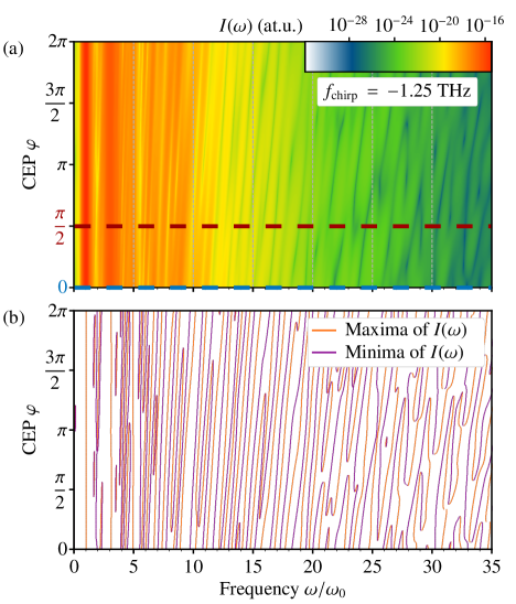
Figure 2: (a) High-harmonics spectrum $I(\omega)$ computed from SBE, Eq. (5) for 384 discrete CEPs $\varphi\hskip 1.34995pt{\in}\hskip 1.34995pt[0,2\pi]$ with ${\bf E}(t)$ and parameters as in Fig. 1. The heat map along the blue and red horizontal line (CEP $\varphi\hskip 1.52998pt{=}\hskip 1.52998pt0$ and $\varphi\hskip 1.52998pt{=}\hskip 1.52998pt\pi/2$) represents the emission spectra from Fig. 1. (b) Local extrema of $I(\omega)$ from (a).

The resulting high-harmonics spectrum $I(\omega)$ for pulse parameters adapted to experiment [10] is shown in Fig. 1, for a sine-like pulse ($\varphi\hskip 1.69998pt{=}\hskip 1.69998pt0$) and a cosine-like pulse ($\varphi\hskip 1.69998pt{=}\hskip 1.69998pt\pi/2$): Both high-harmonics spectra are similar up to fifth harmonic order, $\nu\hskip 1.69998pt{=}\hskip 1.69998pt5$, using a dimensionless frequency $\nu\hskip 1.69998pt{\coloneqq}\hskip 1.69998pt\omega/\omega_{0}$. At higher frequencies, $14\hskip 1.69998pt{\lesssim}\hskip 1.69998pt{\nu}\hskip 1.69998pt{\lesssim}\hskip 1.69998pt20$, the two spectra differ in the sense that the maximum of one coincides with the minimum of the other. At even higher frequencies, $30\hskip 1.69998pt{\lesssim}\hskip 1.69998pt{\nu}\hskip 1.69998pt{\lesssim}\hskip 1.69998pt35$, maxima of the two spectra coincide and minima also coincide.

Similar to the experiment, [10] we continuously vary the CEP from 0 to $2\pi$, see Fig. 2 (a) and (b). We confirm the main experimental findings, albeit here observed in a much larger window, $5\hskip 1.69998pt{\lesssim}\hskip 1.69998pt\nu\hskip 1.69998pt{\lesssim}\hskip 1.69998pt35$, instead of $12\hskip 1.69998pt{\lesssim}\hskip 1.69998pt\nu\hskip 1.69998pt{\lesssim}\hskip 1.69998pt21$ in Ref. 10: The frequency shift grows at increasing harmonic order, which eventually leads to a pattern of tilted lines with tilt angle growing from left to right in Fig. 2 (b). Indications of an increase of the tilt-angle have been observed before in semiconductors and dielectrics, but the patterns there are less pronounced and systematical. [11] Presumably this is why a systematic theoretical understanding predicting parametric dependencies of CEP shifts has not been worked out.

IV CEP shifts for a semiclassical model – analytical formula

The systematic growth of the tilt angle with the high-harmonic order seen in Fig. 2 (b) suggests that there should be a simple analytical formula characterizing parametric dependencies. In this section such a formula is derived within a minimal model.

We employ a semiclassical framework [65] neglecting anomalous velocity contributions. [66] Within this model, the electron velocity is given by

$$\mathbf{v}(t)=\left.\frac{\partial\epsilon}{\hbar\,\partial\mathbf{k}}\right|_{\mathbf{k}=\mathbf{k}(t)}\,.$$ (6)

$\mathbf{k}(t)$ is the excursion of the electron in reciprocal space. In semiclassics, $\mathbf{k}(t)$ fully characterizes the dynamics of the electron and is given by the Bloch acceleration theorem [67]

$$\mathbf{k}(t)=\mathbf{k}_{0}+\frac{1}{\hbar}\int\limits^{t}_{-\infty}{\bf F}(t^{\prime})\,dt^{\prime}\,,$$ (7)

where ${\bf F}$ is the acting force, ${\bf F}(t)\hskip 1.69998pt{=}\hskip 1.69998pt{-}e\hskip 0.50003pt{\bf E}(t)$, if only electric fields are to be accounted for. In our simplified approach we assume that the time dependence of ${\bf j}(t)$ is captured by $\mathbf{v}(t)$ taken at a characteristic wavenumber $\mathbf{k}_{0}$. For the purpose of calculating CEP shifts, prefactors - such as effective charge densities - can be ignored since they cancel for CEP shifts in Eq. (3).

We now analyze CEP shifts within the framework of model (6) and (7). Since it is assumed ${\bf j}(t)\hskip 1.69998pt{\propto}\hskip 1.69998pt\mathbf{v}(t)$, we have

$$I(\omega)\hskip 1.69998pt{\propto}\hskip 1.69998pt\omega^{2}|\mathbf{v}(\omega)|^{2}=|\partial_{t}\mathbf{v}(\omega)|^{2}$$ (8)

from Eq. (5), where

$$\partial_{t}\mathbf{v}(\omega)\coloneqq\int dt\ e^{-{i}\omega t}\ \partial_{t}\mathbf{v}(t)=\int dt\ e^{-{i}\omega t}\ \partial_{t}\left.\frac{\partial\epsilon}{\hbar\,\partial\mathbf{k}}\right|_{\mathbf{k}(t)}$$ (9)

is the Fourier transform of the time-dependent acceleration.

If the $\mathbf{k}$-derivative is analytic in the range of excursion of $\mathbf{k}(t)$, we may simplify

$$\partial_{t}\hskip 0.50003ptv_{i}\hskip 0.50003pt(\omega) =\sum_{j}\int dt\ e^{-{i}\omega t}\left.\frac{\partial^{2}\epsilon}{\hbar\,\partial k_{i}\hskip 0.50003pt\partial k_{j}}\right|_{\mathbf{k}=\mathbf{k}(t)}\partial_{t}k_{j}\hskip 0.50003pt(t)$$

$$=-\frac{e}{\hbar}\sum_{j}\int dt\ e^{-{i}\omega t}\left.\frac{\partial^{2}\epsilon}{\hbar\,\partial k_{i}\hskip 0.50003pt\partial k_{j}}\right|_{\mathbf{k}=\mathbf{k}(t)}E_{j}\hskip 0.50003pt(t).$$

where we have $\partial_{t}k_{j}\hskip 0.50003pt(t)\hskip 1.69998pt{=}\hskip 1.69998pt{-}\hskip 0.50003pteE_{j}\hskip 0.50003pt(t)/\hbar$ in the absence of magnetic fields. It is a necessary condition for the generation of high harmonics that $\partial^{2}\epsilon/(\partial k_{i}\partial k_{j})|_{\mathbf{k}=\mathbf{k}(t)}$ is time dependent. For the special case of parabolic dispersions with isotropic effective mass $m$ we obtain

$$\partial_{t}\mathbf{v}(\omega) =-\frac{e}{m}\,{\bf E}(\omega)\,.$$

The conclusion is that parabolic dispersions do not exhibit HHG (within the validity of our minimal model) [68].

As a minimal model for Dirac fermions we consider a linear dispersion

$$\epsilon(\mathbf{k})=\hbar v_{\text{F}}\hskip 0.50003pt|\mathbf{k}|\,.$$ (10)

The velocity (6) for the linear dispersion is

$$\mathbf{v}(t)=\hat{\mathbf{x}}\,v_{\text{F}}\,\text{sgn}(k_{x}(t))\,;$$ (11)

the velocity is a constant, $v_{\text{F}}$, and it only changes its sign when $k_{x}(t)$ crosses zero. Hence, the acceleration $\partial_{t}\mathbf{v}(t)$ is a sequence of $\delta$-functions in time with a corresponding Fourier transform

$$\partial_{t}\mathbf{v}(\omega)=\sum_{m=1}^{N_{z}}\mathbf{v}_{m}\exp(i\omega t_{m})\,,$$ (12)

where $\mathbf{v}_{m}\hskip 1.69998pt{=}\hskip 1.69998pt2v_{\text{F}}\,(-1)^{m+1}\,\hat{\mathbf{x}}$ for the linear dispersion (10). The summation is over the zeros $t_{m}$ of $k_{x}(t)$, which are readily obtained from (7); $N_{z}$ denotes the number of these zeros (see App. B for a formal derivation.) The zeros $t_{m}$ will shift in the presence of a CEP, $t_{m}(\varphi)$. Since we require a $2\pi$-periodicity in $\varphi$, we have $t_{m}(\pm 2\pi)\hskip 1.69998pt{=}\hskip 1.69998ptt_{m\pm p}(0)$, so after a full rotation a root $m$ shifts into root $m\hskip 1.69998pt{\pm}\hskip 1.69998ptp$, $p$ being integer. 

Eq. (12) is expected to be applicable to broader classes of band-structures, the main requirement is a sufficiently large frequency $\omega$. Indeed, high-harmonic radiation consistent with (12) has been observed in experiments on semiconductors [4]. We show in detail that the following analysis also applies to the general case, Eq. (12) in App. E.

The emission intensity (8) corresponding to (12) for the linear dispersion (10) with $\mathbf{v}_{m}\hskip 1.69998pt{=}\hskip 1.69998pt2v_{\text{F}}\,(-1)^{m+1}\,\hat{\mathbf{x}}$ reads

$$I(\omega)\propto|\partial_{t}\mathbf{v}(\omega)|^{2}\propto\sum_{\ell,m}^{N_{z}}(-1)^{\ell+m}e^{i\omega\hskip 0.35002ptt_{\ell m}(\varphi)}\,,$$ (13)

with $t_{\ell m}(\varphi)\hskip 1.69998pt{\coloneqq}\hskip 1.69998ptt_{\ell}(\varphi)\hskip 1.69998pt{-}\hskip 1.69998ptt_{m}(\varphi)$. Then, Eq. (3) readily implies

$$\frac{d\omega}{d\varphi}=-\,\omega\,\frac{I_{t}^{\prime}}{I_{t}}$$ (14)

where

$$I_{t}(\omega,\varphi) \coloneqq\sum_{\ell,m}^{N_{z}}(-1)^{\ell+m}e^{i\omega t_{\ell m}(\varphi)}t_{\ell m}(\varphi)\,,$$ (15)

$$I_{t}^{\prime}(\omega,\varphi) \coloneqq\sum_{\ell,m}^{N_{z}}(-1)^{\ell+m}e^{i\omega t_{\ell m}(\varphi)}\partial_{\varphi}t_{\ell m}(\varphi)\,.$$ (16)

As an application, we consider the situation in which the CEP $\varphi$ induces a homogeneous shift of all roots: $t_{m}(\varphi)\hskip 1.69998pt{=}\hskip 1.69998ptt_{m}(0)\hskip 1.69998pt{+}\hskip 1.69998pt\varphi/\omega_{0}$ and, in addition, an equidistant spacing $t_{m}(\pi)\hskip 1.69998pt{=}\hskip 1.69998ptt_{m+1}(0)$. Here implied is that $t_{\ell m}(\varphi)$ is independent of $\varphi$ and therefore $I_{t}^{\prime}\hskip 1.69998pt{=}\hskip 1.69998pt0$. We conclude that a non-vanishing CEP shift requires that the zeros of $\mathbf{k}(t)$ are not equidistantly spaced. 

Non-equidistant roots of $\mathbf{k}(t)$ result from a time-dependent carrier frequency, which is defined as $(1+{\mathfrak{f}}(t))\hskip 0.50003pt\omega_{0}$ (”chirp” ${\mathfrak{f}}(t)$). In the App. C, we show that for small and slowly varying ${\mathfrak{f}}(t)$, Eq. (14) simplifies to

$$\frac{d\omega}{d\varphi}=-\hskip 0.50003pt2\hskip 0.50003pt\frac{\omega}{\omega_{0}}\hskip 0.50003pt\bar{\mathfrak{f}}^{\prime}\,,$$ (17)

where $\bar{\mathfrak{f}}^{\prime}$ is the average slope of ${\mathfrak{f}}(t)$. Eq. (17) is our main result; it implies that under generic conditions the tilt angle $d\omega/d\varphi$ increases linearly in $\omega$, and is independent of $\varphi$.

We now adress the shift of peak frequencies $\omega_{\text{peak}}$ in the high-harmonics spectrum, when changing the CEP from $0$ to $2\pi$, $\Delta\omega_{\text{peak}}\hskip 1.69998pt{\coloneqq}\hskip 1.69998pt{\int_{0}^{2\pi}}d\varphi\,(d\omega/d\varphi)$ along an equi-intensity line $\omega(\varphi)$. In the regime $|\bar{\mathfrak{f}}^{\prime}/\omega_{0}|\hskip 1.69998pt{\ll}\hskip 1.69998pt1$ we focus on, $d\omega/d\varphi$ is only weakly dependent on the integration variable, because the relative change of $\omega(\varphi)$ along the equi-potential line is small: $\Delta\omega_{\text{peak}}\hskip 1.69998pt{\ll}\hskip 1.69998pt\omega_{\text{peak}}$; we thus approximate on the rhs of (17) $\omega\hskip 0.50003pt(\varphi)\hskip 1.69998pt{\approx}\hskip 1.69998pt\hskip 0.50003pt\omega\hskip 0.50003pt(\varphi\hskip 1.69998pt{=}\hskip 1.69998pt0)\hskip 1.69998pt{=}\hskip 1.69998pt\omega_{\text{peak}}$, and arrive at the peak shift

$$\Delta\omega_{\text{peak}}=-\,4\pi\,\frac{\omega_{\text{peak}}}{\omega_{0}}\,\bar{\mathfrak{f}}^{\prime}\,.$$ (18)

As an application of Eqs. (17) and (18), we consider an archetypical electric-field pulse (4), implying $\bar{\mathfrak{f}}^{\prime}\hskip 1.69998pt{=}\hskip 1.69998ptf_{\text{chirp}}$, and small filling, i.e., $k_{\text{F}}$ far away from all Brillouin zone boundaries, motivating a non-vanishing $|\mathbf{k}_{0}|\hskip 1.69998pt{\lesssim}\hskip 1.69998ptk_{\text{F}}$. In this case the number of roots of $\mathbf{k}(t)$, $N_{z}$, is bounded: at infinite times the integral in (7) vanishes (since ${\bf E}(\omega\hskip 1.69998pt{=}\hskip 1.69998pt0)\hskip 1.69998pt{=}\hskip 1.69998pt0$) so that $\mathbf{k}(t)$ takes a non-vanishing limiting value.

Eq. (17) takes a simple form; while the frequency $\omega$ and the detuning per period $\bar{\mathfrak{f}}^{\prime}/\omega_{0}$ enter, other material or system parameters do not. The absence of $v_{\text{F}}$ follows from the fact that the CEP is given as an intensity ratio, Eq. (3). Similarly, the envelope parameter $\sigma$ of the driving electric field (4) (parameterized via $N_{z}$) cancels since our approximations imply $I_{t}^{\prime}\hskip 1.69998pt{\propto}\hskip 1.69998ptI_{t}$.

The linear dependency of $d\omega$ on the chirp parameter $\bar{\mathfrak{f}}^{\prime}$ is rationalized as follows: By definition, the chirp accounts for the non-linear spacing of the roots of $\mathbf{k}(t)$. Therefore, in the absence of chirp, the CEP translates all roots by the same amount and therefore can be eliminated by a redefinition of the origin of time, $t\hskip 1.49994pt{\rightarrow}\hskip 1.49994ptt\hskip 1.69998pt{-}\hskip 1.69998ptd\varphi/\omega_{0}$. Thus, at $\bar{\mathfrak{f}}^{\prime}\hskip 1.69998pt{=}\hskip 1.69998pt0$ the current and the emission spectrum are both independent of $\varphi$ resulting in the absence of CEP shifts, $d\omega\hskip 1.69998pt{=}\hskip 1.69998pt0$ (cf. App. D). At non-vanishing chirp, corrections arise already at linear-order, $d\omega\hskip 1.69998pt{\propto}\hskip 1.69998pt\bar{\mathfrak{f}}^{\prime}$, reflecting the fact that the tilt $d\omega/d\varphi$ can take either sign.

Finally, the proportionality $d\omega\hskip 1.69998pt{\propto}\hskip 1.69998pt\omega/\omega_{0}$ can be understood by recalling that the electrons perform a number of $\omega/\omega_{0}$ cycles during a single fundamental period of $E(t)$. They thus can be expected to be more sensitive to a parametric change in $E(t)$, for example a change of $\bar{\mathfrak{f}}^{\prime}$, by a factor of $\omega/\omega_{0}$.

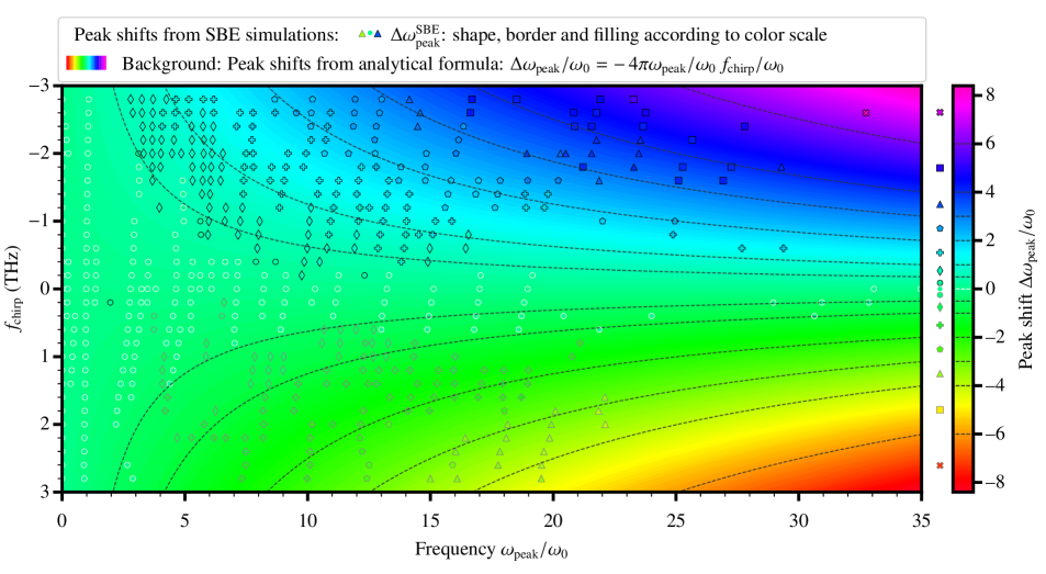
Figure 3: Quantitative comparison of the peak shifts as obtained from the analytical formula (18) (background, $\Delta\omega_{\text{peak}}$) and from SBE simulations (color-filled circles, $\Delta\omega_{\text{peak}}^{\text{SBE}}$) in the parameter plane $(\omega_{\text{peak}},f_{\text{chirp}})$. $\Delta\omega_{\text{peak}}^{\text{SBE}}$ are obtained by tracing continuous maximum lines of the emission $I(\omega)$ as shown in Fig. 2 (b) from the initial point $(\omega_{\text{peak}}^{\text{{SBE}}},\varphi\hskip 1.52998pt{=}\hskip 1.52998pt0)$ to the final point $(\omega_{\text{peak}}^{\text{{SBE}}}\hskip 1.52998pt{+}\hskip 1.52998pt\Delta\omega_{\text{peak}}^{\text{{SBE}}},\varphi\hskip 1.52998pt{=}\hskip 1.52998pt2\pi)$. The dashed lines are guiding the eye; they indicate constant $\Delta\omega_{\text{peak}}$ in the analytical formula. (For the SBE simulations, we considered 29 chirps with 384 CEPs each resulting in 11136 SBE runs.)

V comparison of the analytical formula to SBE simulations

We proceed with a comparison of the analytical formulæ (17), (18) to SBE simulations. In Fig. 2 we display SBE simulations of the CEP-dependent high-harmonic spectra. A straight-line character of the extremal lines – and correspondingly also the equi-intensity lines – is seen which is synonymous with a minor tilt-angle dependency on CEP $\varphi$; further the tilt angle $d\omega/d\varphi$ increases with $\omega$. Both observations are fully consistent with our main result, Eq. (17).

With respect to the sign of the tilt, we further observe in Fig. 2 that the extremal lines are tilted to the right (from south west to north east) which implies a positive tilt angle, $d\omega/d\varphi\hskip 1.69998pt{\geq}\hskip 1.69998pt0$. The positive sign of the tilt angle is consistent with the analytical prediction (17): we evaluate for the pulse (4) the chirp $\bar{\mathfrak{f}}^{\prime}\hskip 1.69998pt{=}\hskip 1.69998ptf_{\text{chirp}}\hskip 1.69998pt{=}\hskip 1.69998pt{-}\hskip 0.50003pt1.25\,$THz implying $d\omega/d\varphi\hskip 1.69998pt{\geq}\hskip 1.69998pt0$ (for $\omega\hskip 1.69998pt{\geq}\hskip 1.69998pt0$).

The high-harmonic spectra reported in Fig. 2 have been generated for a specific choice of the pulse parameters pulse duration $\sigma$, frequency $\omega$, chirp $f_{\text{chirp}}$, field strength $E_{0}$, and the dephasing time $T_{2}$ [71, 59]. We provide an extended set of CEP-dependent high-harmonic spectra in App. H, Figs. 7 – 11, where we change the pulse parameters and we also use two generic semiconductor Hamiltonians instead of the Dirac-type band structure. In all spectra, we observe that the tilt angles follow our analytical results (17) and (18). This finding is in line with the derivation of (17) and (18), that holds independently of a specific band structure or specific pulse shapes.

For a quantitative comparison, we focus on peak shifts $\Delta\omega_{\text{peak}}$. From the SBE simulations shown in Fig. 2 (b) we extract peak shifts by tracing continuous maximum lines (”percolating lines”) of the emission $I(\omega)$ connecting the points in the parameter plane $(\omega_{\text{peak}}^{\text{SBE}},\varphi\hskip 1.69998pt{=}\hskip 1.69998pt0)$ and $(\omega_{\text{peak}}^{\text{SBE}}\hskip 1.69998pt{+}\hskip 1.69998pt\Delta\omega_{\text{peak}}^{\text{SBE}},\varphi\hskip 1.69998pt{=}\hskip 1.69998pt2\pi)$. We obtain pairs of $(\Delta\omega_{\text{peak}}^{\text{SBE}}/\omega_{\text{peak}}^{\text{SBE}})$ as (1.0/10.2), (1.6/19.7), (2.2/24.7). Based on equation (18) we expect a ratio $\Delta\omega_{\text{peak}}/\omega_{\text{peak}}\hskip 1.69998pt{=}\hskip 1.69998pt{-}\hskip 0.50003pt4\pi\bar{\mathfrak{f}}^{\prime}/\omega_{0}\hskip 1.69998pt{=}\hskip 1.69998pt0.1$, in good quantitative agreement with the extracted SBE data (simulation parameters: $\omega_{0}\hskip 1.69998pt{=}\hskip 1.69998pt2\pi\hskip 1.69998pt{\cdot}\hskip 1.69998pt25$ THz and $\bar{\mathfrak{f}}^{\prime}\hskip 1.69998pt{=}\hskip 1.69998ptf_{\text{chirp}}\hskip 1.69998pt{=}\hskip 1.69998pt{-}\hskip 0.50003pt1.25$ THz). We proceed and calculate the peak shifts $\Delta\omega_{\text{peak}}$ for a collection of chirps to test the limits of (18) in the plane spanned by $\omega_{\text{peak}}$ and $f_{\text{chirp}}$. Fig. 3 shows the (color-coded) analytical result (18). The color-filled circles superimposed to the colored, analytical ”background” indicate the corresponding SBE results, $\Delta\omega_{\text{peak}}^{\text{SBE}}$; the circle-colors follow the same scale abopted also for the analytical data.

In Fig. 3, we observe that SBE peak shifts (circles) are in good overall quantitative agreement with the analytical prediction (background): the color of the circular discs matches the background. (Averaging over the entire plane, we compute a mean absolute deviation of only 0.21 $\omega_{0}$.)

At weak chirp and small peak frequencies (low harmonics), the SBE-simulations exhibit many vertical maximum-intensity lines; the corresponding peak shifts vanish. These vanishing peak shifts appear in a region in the phase diagram Fig. 3, which reveals itself as the area that supports light gray circles. The region has a characteristic boundary corresponding to $|\Delta\omega_{\text{peak}}|\hskip 1.69998pt{\leq}\hskip 1.69998pt0.5\,\omega_{0}$; it is indicated by dashed lines in Fig. 3. Within this region, the relative discrepancy to our analytical formula (18) is somewhat enhanced. Outside this region, we find the mean relative absolute deviation in the peak shift to be only 17 % between SBE simulations and the analytical formula (18).

VI comparison of the analytical formula to experiments

We compare our findings (17) and (18) to the experimental high-harmonics spectra emitted from the topological surface state of Bi₂Te₃ [10], reproduced in Fig. 4. This data displays the characteristic stripe pattern that our theoretical analysis predicts. Beyond this, there is also a qualitative agreement in details; e.g., the increase of the tilt angle with growing harmonic order predicted in (17) is also seen in Fig. 4.

For a quantitative analysis, we fit parabolæ

$$\omega(\varphi)\hskip 1.69998pt{=}\hskip 1.69998pt\omega_{0}[\alpha\hskip 1.69998pt{+}\hskip 1.69998pt\beta(\varphi\hskip 1.69998pt{-}\hskip 1.69998pt\bar{\varphi})\hskip 1.69998pt{+}\hskip 1.69998pt\gamma(\varphi\hskip 1.69998pt{-}\hskip 1.69998pt\bar{\varphi})^{2}]$$ (19)

to discrete local maxima with fit parameters $\alpha,\beta,\gamma$ and fixed $\omega_{0},\bar{\varphi}$, see Fig. 4 and caption. We find that the linear term $\beta$ (reported in Table 1) is dominating the fit, in line with our analytical result (17). From our quantitative analysis, we also find that tilt angles tend to increase with the frequency, see Table 1. From 14th to 19th order we observe a ”locking”, i.e., the average tilt angle between 15th and 18th harmonic order changes within 3 %, only (Table 1). This locking is a manifestation of an equidistant placement of the maxima. They reflect combined properties of pulse shape and band structure, that are not captured in our simplified analytical model, but prevail in SBE simulations. Hence, it is not surprising that locking effects also appear in Fig. 2.

The linear coefficient $\beta$ together with the analytical result (17) provides an estimate for the pulse-shape parameter, $2\pi\bar{\mathfrak{f}}^{\prime}/\omega_{0}\hskip 1.69998pt{=}\hskip 1.69998pt{-}\hskip 0.50003pt0.067\pm 0.001$. The experimental pulse shape has been reported in Ref. [10], so that $\bar{\mathfrak{f}}^{\prime}$ can be directly calculated for the given pulse as $2\pi\bar{\mathfrak{f}}^{\prime}/\omega_{0}\hskip 1.69998pt{\approx}\hskip 1.69998pt-0.037$, see App. G; this is half the fitted value. Given that the experimental pulse shape is parametrically not even close to the regime of applicability of the analytical formula (17) – the experimental curvature ${\mathfrak{f}}^{\prime\prime}(t)$ is far from negligible, see App. G for a detailed analysis – we find the semi-quantitative agreement encouraging.

So far, our focus has been on topological surface states of 3D topological insulators. Ref. [10] reports harmonic orders up to 13th emananating also from the semiconducting bulk of the topological insulator Bi₂Te₃. We now compare our analytical results with this experiment. For the pulse shape used in the bulk measurement, we evaluate a tiny chirp $2\pi\bar{\mathfrak{f}}^{\prime}/\omega_{0}\hskip 1.69998pt{\approx}\hskip 1.69998pt{-}\,0.007$ (cf. App. G). Inserting that chirp into our CEP shift formula (17), we predict a slope $d\omega/d\varphi\hskip 1.69998pt{=}\hskip 1.69998pt0.11\omega_{0}/(2\pi)$ for $\omega\hskip 1.69998pt{=}\hskip 1.69998pt8\omega_{0}$. This shift is about 5% of the shift for the topological surface state, which is qualitatively consistent with the experiment: indeed, a small, but non-vanishing slopes can be identified close to the eighth harmonic order [10].

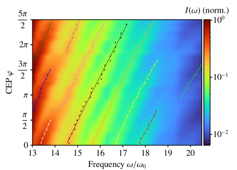
Figure 4: CEP-dependency of the high-harmonics spectrum of Bi₂Te₃; experimental data taken from Ref. [10]. We report local maxima as colored dots. We form sets of local maxima, as indicated by the various colors. For each set, we perform a quadratic fit $\omega(\varphi)\hskip 1.52998pt{=}\hskip 1.52998pt\omega_{0}[\alpha\hskip 1.52998pt{+}\hskip 1.52998pt\beta(\varphi\hskip 1.52998pt{-}\hskip 1.52998pt\bar{\varphi})\hskip 1.52998pt{+}\hskip 1.52998pt\gamma(\varphi\hskip 1.52998pt{-}\hskip 1.52998pt\bar{\varphi})^{2}]$ (dotted lines, $\bar{\varphi}$ is fixed as the average CEP of a line segment, fit parameters $\alpha,\beta,\gamma$ are reported in Tables 1,2).

Table 1: Fit parameter $\beta$ (tilt angle) of fits reported in Fig. 4, as function of the average frequency $\bar{\omega}$ of the line segment. We report the full set of fit parameters in App. F.

$\bar{\omega}/\omega_{0}$	13.4	13.5	13.6	14.8	15.3	15.8	17.0	17.5	18.1	20.1
$2\pi\beta$	1.81	2.00	1.89	1.86	2.23	2.25	2.19	2.24	2.39	2.84

VII Conclusion

We propose an analytical theory for the carrier envelope phase (CEP) dependency of high-harmonic generation under illumination of a material with strong laser pulses. The central result is a simple analytical formula describing the shifts of high-harmonic peaks under the change of the CEP. This formula explains, e.g., why peak positions can occur at non-integer harmonic orders. Further, it predicts that the shift velocity is proportional to the peak frequency and the chirp of the driving laser pulse. The comparison with a full-fledged simulation based on the semiconductor-Bloch formalism establishes the quantitative accuracy of the analytical result in a large parameter regime. Also the comparison to the experiment [10] is surprisingly favorable given that the experimental pulse shape is only marginally consistent with the conditions of applicability of our formula.

Our theory provides the first understanding of the phenomenon of CEP shifts in materials based on simple, analytically derived parametric dependencies. We conclude emphasizing the broad applicability of our result, the validity of which we have demonstrated for a large parameter regime and a wide range of material classes. Our work represents another stepping stone towards understanding the microscopic mechanisms underlying high-harmonic generation in materials.

Code availability

For all SBE simulations, we have used our program package CUED [59], that is freely available, https://github.com/ccmt-regensburg/CUED.

Author contributions

M.G. carried out SBE simulations and analyzed the numerical data. M.N, M.G., F.E., and J.W. developed the analytical model. A.S. developed the SBE simulation code. F.E. and J.W. conceived the study, supervised the project and wrote the paper with contributions from all authors. All authors contributed to discussing the results.

Appendix A Computational details and convergence tests

As electric field, we use Eq. (4) throughout where the parameters $E_{0}\hskip 1.69998pt{=}\hskip 1.69998pt3\,\mathrm{MV/cm}$, $\omega_{0}\hskip 1.69998pt{=}\hskip 1.69998pt2\pi\hskip 1.69998pt{\cdot}\hskip 1.69998pt25\,\mathrm{THz}$ and $\sigma\hskip 1.69998pt{=}\hskip 1.69998pt90\,\mathrm{fs}$ were fixed for the calculations in the main text. We align the electric field along the $\Gamma$-M direction which we label as $x$-direction in Eq. (4). We have used the two-band Dirac-like model Hamiltonian for the topological surface states of Bi₂Te₃ from Ref. [10] together with a hexagonal Brillouin zone with a size that stems from a real space lattice constant $a\hskip 1.69998pt{=}\hskip 1.69998pt4.396\,\AA$. As in Ref. [10], we start from an equilibrium band occupation that is given by a Fermi-Dirac distribution with a Fermi level of 0.176 eV above the conduction band minimum and with a temperature of 30 meV. We compute the time-dependent density matrix $\rho(t)$ from SBE in the velocity gauge with a dephasing time $T_{2}\hskip 1.69998pt{=}\hskip 1.69998pt10$ fs which is an accepted simulation value [71]. For the time evolution in the SBE formalism, we employ an adaptive algorithm [72] with a maximum time step of $0.1$ fs and with a time window of $[-500\,\text{fs},500\,\text{fs}]$. These settings lead to intensity spectra that are converged with respect to time discretization. The Fourier transform to frequency domain includes a Gaussian window function with full width at half maximum of $2\sqrt{\ln 2}\cdot 90$ fs. In the SBE, dipoles are used which are diverging for the Dirac-like two-band Hamiltonian at the $\Gamma$-point [73, 59]. Thus, we carefully checked the convergence of the $k$-point mesh, see Fig. 5.

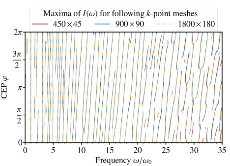
Figure 5: Maxima of $I(\omega)$ computed with parameters as in Fig. 2 c for three different Monkhorst-Pack $k$-point meshes [74] $N_{1}\hskip 1.26pt{\times}\hskip 0.80997ptN_{2}$ ($450\hskip 1.26pt{\times}\hskip 0.80997pt45,900\hskip 1.26pt{\times}\hskip 0.80997pt90,1800\hskip 1.26pt{\times}\hskip 0.80997pt180$), where $N_{1}$ is the number of $k$-points in $\Gamma$-M direction and $N_{2}$ is the number of $k$-points orthogonal to the $\Gamma$-M direction.

We observe excellent agreement between the $900\hskip 1.4pt{\times}\hskip 0.89996pt90$ and $1800\hskip 1.4pt{\times}\hskip 0.89996pt180$ $k$-mesh. We conclude that the $900\hskip 1.4pt{\times}\hskip 0.89996pt90$ mesh is sufficient to reach convergence in the $k$-point mesh size and therefore, we have used a $900\hskip 1.4pt{\times}\hskip 0.89996pt90$ mesh for all SBE calculations. In all figures, we have varied the CEP from 0 to $2\pi$, where we have used $N_{\text{CEP}}\hskip 1.69998pt{=}\hskip 1.69998pt384$ discrete CEPs in the $[0,2\pi]$ window thoughout.

Appendix B Fourier transform of the time-dependent current

The time derivative of the current (11) is

$$\partial_{t}\mathbf{v}(t)=-\,2\,\hat{\mathbf{x}}\,\frac{ev_{\text{F}}}{\hbar}\,E(t)\;\delta(\hskip 0.50003ptk_{x}(t)\hskip 0.50003pt)\,,$$ (20)

where $\delta$ denotes the Dirac delta function. Then,

$$\delta(\hskip 0.50003ptk_{x}(t)\hskip 0.50003pt) =\sum_{m}\frac{\delta(t-t_{m}(\varphi))}{\left|\left.\partial_{t}k_{x}(t)\right|_{t_{m}(\varphi)}\right|}=\sum_{m}\frac{\delta(t-t_{m}(\varphi))}{e\left|E(t_{m}(\varphi))\right|/\hbar}\,.$$ (21)

Combining Eqs. (20) and (21), we arrive at Eq. (12),

$$\mathbf{v}(\omega)=\frac{1}{i\omega}\,\partial_{t}\mathbf{v}(\omega)=\frac{2v_{\text{F}}}{i\omega}\;\hat{\mathbf{x}}\sum_{m}(-1)^{m+1}\exp[i\omega t_{m}(\varphi)]\,.$$ (22)

The linear dispersion (10) of the model band structure is justified by the Dirac character of the surface conduction band of Bi₂Te₃ close to the $\Gamma$-point [64]. For the other commonly adopted model band structure, a parabolic dispersion $\epsilon(\mathbf{k})\hskip 1.69998pt{=}\hskip 1.69998pt\hbar^{2}|\mathbf{k}|^{2}/(2m)$, no high-harmonic emission is observed under driving by an electric field from Eq. (4). This is due to the velocity $\mathbf{v}(t)\hskip 1.69998pt{=}\hskip 1.69998pt\hbar\mathbf{k}(t)/m$ [Eq. (6)] oscillating solely with the fundamental frequency $\omega_{0}$.

We also do not consider excitonic effects and other electron-electron interaction during the non-equilibrium dynamics as they are believed to have negligible contributions [10]. Also, we omit bulk bands which have been shown to not contribute to the high-harmonic emission for the pulse shape we consider in this work [10].

Appendix C General discussion of CEP-shifts at weak chirp

We give more details on the discussion of the spacing of roots in Sec. IV. The starting point is a homogeneous spacing, $t^{(0)}_{m}(\varphi)\hskip 1.69998pt{=}\hskip 1.69998pt(m\pi\hskip 1.69998pt{-}\hskip 1.69998pt\varphi)/\omega_{0}$ of the zeros of (7), $\mathbf{k}(t^{(0)}_{m}(\varphi))\hskip 1.69998pt{=}\hskip 1.69998pt0$, where $\omega_{0}$ is the fundamental frequency. We achieve a non-uniform spacing by implementing a small rescaling of the time, $\mathbf{k}(t)\hskip 1.49994pt{\rightarrow}\hskip 1.49994pt\mathbf{k}\big{(}t(1\hskip 1.69998pt{+}\hskip 1.69998pt{\mathfrak{f}}(t)\big{)}$, such that we have for the zeros $t_{m}(\varphi)$ with non-uniform spacing

$$t_{m}^{(0)}(\varphi)=\Big{[}\hskip 0.50003pt1+{\mathfrak{f}}(t_{m}(\varphi))\hskip 0.50003pt\Big{]}\,t_{m}(\varphi)\,.$$ (23)

The chirp introduced in Sec. IV corresponds to a linear dependency ${\mathfrak{f}}(t)\hskip 1.69998pt{=}\hskip 1.69998ptf_{\text{chirp}}t$. We consider more general situations subject to the condition that ${\mathfrak{f}}(t)$ is slowly varying from one zero to the next. Solving (23) for $t_{m}$ we have

$$t_{m}(\varphi) =t^{(0)}_{m}(\varphi)-{\mathfrak{f}}(t^{(0)}_{m}(\varphi))\ t^{(0)}_{m}(\varphi)+\mathcal{O}({\mathfrak{f}}^{2})$$

$$\approx t^{(0)}_{m}(\varphi)\left[1-{\mathfrak{f}}(t^{(0)}_{m}(\varphi))\right]$$ (24)

where gradient terms have been neglected. Further, after defining the equal spacing ($t^{(0)}_{\ell m}\hskip 1.69998pt{\coloneqq}\hskip 1.69998ptt^{(0)}_{\ell}(\varphi)\hskip 1.69998pt{-}\hskip 1.69998ptt^{(0)}_{m}(\varphi)\hskip 1.69998pt{=}\hskip 1.69998pt\pi(\ell\hskip 1.69998pt{-}\hskip 1.69998ptm)/\omega_{0}\hskip 1.69998pt{=}\hskip 1.69998ptt^{(0)}_{\ell-m}(\varphi{=}0)$), we define the non-uniform spacing $t_{\ell m}(\varphi)\hskip 1.69998pt{\coloneqq}\hskip 1.69998ptt_{\ell}(\varphi)\hskip 1.69998pt{-}\hskip 1.69998ptt_{m}(\varphi)$

$$t_{\ell m}(\varphi) \approx t^{(0)}_{\ell m}-\left[t^{(0)}_{\ell}(\varphi)\,{\mathfrak{f}}(t^{(0)}_{\ell}(\varphi))-t^{(0)}_{m}(\varphi)\,{\mathfrak{f}}(t^{(0)}_{m}(\varphi))\right]$$

$$\approx t^{(0)}_{\ell m}\left[1-{\mathfrak{f}}(T^{(0)}_{\ell m}(\varphi))-T^{(0)}_{\ell m}(\varphi)\,{\mathfrak{f}}^{\prime}(T^{(0)}_{\ell m}(\varphi))\right]$$ (25)

where $T^{(0)}_{\ell m}(\varphi)\hskip 1.69998pt{\coloneqq}\hskip 1.69998pt(t^{(0)}_{\ell}(\varphi)\hskip 1.69998pt{+}\hskip 1.69998ptt^{(0)}_{m}(\varphi))/2\hskip 1.69998pt{=}\hskip 1.69998ptt^{(0)}_{(\ell+m)/2}(\varphi)$ and terms involving second derivatives have been dropped. Similarly, we have

$$\partial_{\varphi}t_{\ell m} =2t^{(0)}_{\ell m}\,{\mathfrak{f}}^{\prime}(T^{(0)}_{\ell m})/\omega_{0}$$ (26)

and Eqs. (15) and (16) are therefore to leading order in ${\mathfrak{f}}$

$$I_{t}(\omega) =\sum_{\ell,m}^{N_{z}}(-1)^{\ell+m}e^{i\omega t^{(0)}_{\ell m}}\ t^{(0)}_{\ell m}\,,$$ (27)

$$I_{t}^{\prime}(\omega,\varphi) =\frac{2}{\omega_{0}}\sum_{\ell,m}^{N_{z}}(-1)^{\ell+m}e^{i\omega t^{(0)}_{\ell m}}\ t^{(0)}_{\ell m}\ {\mathfrak{f}}^{\prime}(T^{(0)}_{\ell m})\,.$$ (28)

For the situation of an equidistant spacing, the double sum can be reorganized as a sum over pairs. The first summation is over pairs with the same distance, $s\hskip 1.69998pt{=}\hskip 1.69998pt\ell\hskip 1.69998pt{-}\hskip 1.69998ptm$, while the second sum is over the different values $M\hskip 1.69998pt{=}\hskip 1.69998pt(m\hskip 1.69998pt{+}\hskip 1.69998pt\ell)/2$ that these pairs will have

$$I_{t}(\omega) =\sum_{s=-N_{z}+1}^{N_{z}-1}e^{i\omega\mathfrak{t}^{(0)}_{s}}\ \mathfrak{t}^{(0)}_{s}\sum_{M=1+|s|/2}^{N_{z}-|s|/2}(-1)^{2M}$$ (29)

$$I_{t}^{\prime}(\omega,\varphi) =\hskip 0.50003pt\frac{2}{\omega_{0}}\sum_{s=-N_{z}+1}^{N_{z}-1}e^{i\omega\mathfrak{t}^{(0)}_{s}}\ \mathfrak{t}^{(0)}_{s}\sum_{M=1+|s|/2}^{N_{z}-|s|/2}(-1)^{2M}\ {\mathfrak{f}}^{\prime}(t^{(0)}_{M}(\varphi))$$ (30)

where we abbreviated $\mathfrak{t}^{(0)}_{s}\hskip 1.69998pt{\coloneqq}\hskip 1.69998ptt^{(0)}_{s}(\varphi{=}0)\hskip 1.69998pt{=}\hskip 1.69998pt\pi s/\omega_{0}$. Using the relation

$$\sum_{M=1+|s|/2}^{N_{z}-|s|/2}(-1)^{2M}=(-1)^{s}(N_{z}-|s|)$$ (31)

we can simplify

$$I_{t}(\omega) =\frac{\pi}{\omega_{0}}\sum_{s=-N_{z}+1}^{N_{z}-1}e^{i\pi(\omega/\omega_{0}+1)s}\,s\,(N_{z}-|s|)$$ (32)

$$I_{t}^{\prime}(\omega,\varphi) =\frac{2\pi}{\omega_{0}^{2}}\sum_{s=-N_{z}+1}^{N_{z}-1}e^{i\pi(\omega/\omega_{0}+1)s}\,s\,(N_{z}-|s|)\ \bar{\mathfrak{f}}^{\prime}(s;\varphi)\,;$$ (33)

in the last line we have introduced an average chirp

$$\bar{\mathfrak{f}}^{\prime}(s;\varphi) \coloneqq\frac{1}{N_{z}-|s|}\sum_{M=1+|s|/2}^{N_{z}-|s|/2}{\mathfrak{f}}^{\prime}(t^{(0)}_{M}(\varphi))$$ (34)

motivated by the observation that a factor $(-1)^{2M-|s|}$ in the $M$-summation can be replaced by unity. In the special situation where $\bar{\mathfrak{f}}^{\prime}(s,\varphi)$ is independent of $s$ and $\varphi$, we have $I_{t}^{\prime}/I_{t}\hskip 1.69998pt{=}\hskip 1.69998pt\hskip 0.50003pt2\hskip 0.50003pt\bar{\mathfrak{f}}^{\prime}/\omega_{0}$; with Eq. (14), we obtain our main result (17)

$$\frac{d\omega}{d\varphi}=-\hskip 0.50003pt2\hskip 0.50003pt\frac{\omega}{\omega_{0}}\bar{\mathfrak{f}}^{\prime}\,.$$ (35)

In particular, when choosing a sinusoidal pulse (4), the zeros of $\mathbf{k}(t)$ for $\mathbf{k}_{0}\hskip 1.69998pt{=}\hskip 1.69998pt0$ are obtained as

$$t_{m}=\frac{1}{\omega_{0}}\,((m\hskip 0.50003pt{+}\hskip 0.50003pt\frac{1}{2})\,\pi-\varphi)\,(1-\frac{f_{\text{chirp}}}{\omega_{0}}\,((m\hskip 0.50003pt{+}\frac{1}{2}\hskip 0.50003pt)\,\pi-\varphi))\,,$$ (36)

in the limit of small chirp ($|f_{\text{chirp}}|\hskip 1.00006pt{\ll}\hskip 1.00006pt\omega_{0}$) and for small $|m|,m\hskip 1.49994pt{\in}\hskip 1.49994pt\mathbb{Z}$ as it is applicable in case of a few-cycle pulse $E(t)$. When comparing to Eq. (24), we obtain $t^{(0)}_{m}(\varphi)\hskip 1.69998pt{=}\hskip 1.69998pt((m\hskip 1.69998pt{+}\hskip 1.69998pt1/2)\pi\hskip 1.69998pt{-}\hskip 1.69998pt\varphi)/\omega_{0}$, ${\mathfrak{f}}(t^{(0)}_{m}(\varphi))\hskip 1.69998pt{=}\hskip 1.69998ptf_{\text{chirp}}t^{(0)}_{m}(\varphi)$ and $\bar{\mathfrak{f}}^{\prime}\hskip 1.69998pt{=}\hskip 1.69998ptf_{\text{chirp}}$.

Appendix D High-harmonic frequencies for the 1D Dirac dispersion

In this section, we analytically calculate the chirp-free high-harmonic peak frequencies of our semiclassical model from Sec. IV. Following App. C, we have at zero chirp (${\mathfrak{f}}(t)\hskip 1.69998pt{=}\hskip 1.69998pt0$) an equidistant spacing of roots of the electron excursion $\mathbf{k}(t)$ in the Brillouin zone, $t_{\ell m}\hskip 1.69998pt{=}\hskip 1.69998pt\pi(\ell\hskip 1.69998pt{-}\hskip 1.69998ptm)/\omega_{0}$. Then, the emission intensity $I(\omega)$ from Eq. (13) turns into

$$I(\omega)\propto\sum_{\ell,m}^{N_{z}}(-1)^{\ell+m}e^{i(\ell-m)\omega/\omega_{0}}\,.$$ (37)

Using the substitution $s\hskip 1.69998pt{=}\hskip 1.69998pt\ell\hskip 1.69998pt{-}\hskip 1.69998ptm$ and $M\hskip 1.69998pt{=}\hskip 1.69998pt(m\hskip 1.69998pt{+}\hskip 1.69998pt\ell)/2$, we obtain similarly to App. C the emission intensity

$$I(\omega)\propto\Big{(}2N_{z}+\frac{\omega_{0}}{\pi}\frac{\partial}{\partial\omega}\Big{)}\sum_{s=0}^{N_{z}-1}\cos(\pi s(\omega/\omega_{0}+1))$$ (38)

which is independent of the CEP $\varphi$. In the limit $N_{z}\hskip 1.49994pt{\rightarrow}\hskip 1.49994pt\infty$, the sum takes a non-zero value only for $\omega\hskip 1.69998pt{=}\hskip 1.69998pt(2k\hskip 1.69998pt{+}\hskip 1.69998pt1)\,\omega_{0},k\hskip 1.49994pt{\in}\hskip 1.49994pt\mathbb{Z}$. We recover that high-harmonic peaks appear at odd orders in inversion-symmetric materials. ”Non-integer” HHG is therefore only present for non-vanishing chirp, ${\mathfrak{f}}(t)\hskip 1.69998pt{\neq}\hskip 1.69998pt0$, where peak frequencies $\omega$ get shifted according to Eq. (18).

Appendix E CEP shifts for generic band structures

We derive Eqs. (17) and (18) for a more generic situation, where the current needs to fulfill

$$\partial_{t}\mathbf{v}(\omega)=\sum_{m=1}^{N_{z}}\mathbf{v}_{m}\exp(i\omega t_{m}(\varphi))$$ (39)

for high-harmonic frequencies $\omega\hskip 1.69998pt{\gg}\hskip 1.69998pt\omega_{0}$. The time points $t_{m}$ are non-equidistant and are shifted by a linearized slope of ${\mathfrak{f}}(t)\hskip 1.69998pt{=}\hskip 1.69998ptf_{\text{chirp}}t$ according to

$$t_{m}(\varphi)=t^{(0)}_{m}(\varphi)\left[1-f_{\text{chirp}}t^{(0)}_{m}(\varphi)\right]$$ (40)

with equidistant $t^{(0)}_{m}(\varphi)\hskip 1.69998pt{=}\hskip 1.69998pt(m\pi\hskip 1.69998pt{-}\hskip 1.69998pt\varphi)/\omega_{0}$. Starting from our definition of CEP shifts (3), we calculate

$$(\partial I/\partial\omega)_{\varphi} \hskip 1.69998pt{=}\hskip 1.69998pti\sum_{\ell,m}^{N_{z}}\alpha_{\ell m}e^{i\omega t_{\ell m}}t_{\ell m}$$ (41)

$$(\partial I/\partial\varphi)_{\omega} \hskip 1.69998pt{=}\hskip 1.69998pti\omega\sum_{\ell,m}^{N_{z}}\alpha_{\ell m}e^{i\omega t_{\ell m}}\partial_{\varphi}t_{\ell m}\,,$$ (42)

where we have defined $\alpha_{\ell m}\hskip 1.69998pt{\coloneqq}\hskip 1.69998pt\mathbf{v}_{\ell}\cdot\mathbf{v}_{m}^{*}$. The non-uniform time spacings $t_{\ell m}\hskip 1.69998pt{=}\hskip 1.69998ptt_{\ell m}(\varphi)\hskip 1.69998pt{=}\hskip 1.69998ptt_{\ell}(\varphi)-t_{m}(\varphi)$ can be computed as in App. C.

In the spirit of App. C, we reorganize the sums from indices $\ell,\,m$ to $s\hskip 1.69998pt{=}\hskip 1.69998pt\ell\hskip 1.69998pt{-}\hskip 1.69998ptm$ and $M\hskip 1.69998pt{=}\hskip 1.69998pt(m\hskip 1.69998pt{+}\hskip 1.69998pt\ell)/2$. By identifying $\alpha_{sM}\hskip 1.69998pt{=}\hskip 1.69998pt\alpha_{\ell m}$ and using Eq. (26), we obtain in leading order in $f_{\text{chirp}}$:

$$(\partial I/\partial\omega)_{\varphi} \hskip 1.69998pt{=}\hskip 1.69998pti\sum_{s=1-N_{z}}^{N_{z}-1}t^{(0)}_{s}e^{i\omega t^{(0)}_{s}}\sum_{M=1+|s|/2}^{N_{z}-|s|/2}\alpha_{sM}$$ (43)

$$(\partial I/\partial\varphi)_{\omega} \hskip 1.69998pt{=}\hskip 1.69998pti\omega\sum_{s=1-N_{z}}^{N_{z}-1}t^{(0)}_{s}e^{i\omega t^{(0)}_{s}}\sum_{M=1+|s|/2}^{N_{z}-|s|/2}\alpha_{sM}\frac{2}{\omega_{0}}{\mathfrak{f}}^{\prime}(t^{(0)}_{M}(\varphi))\,,$$ (44)

where we use the equidistant spacing $t^{(0)}_{\ell m}\hskip 1.69998pt{=}\hskip 1.69998ptt^{(0)}_{\ell}(\varphi)\hskip 1.69998pt{-}\hskip 1.69998ptt^{(0)}_{m}(\varphi)\hskip 1.69998pt{=}\hskip 1.69998pt\pi(\ell\hskip 1.69998pt{-}\hskip 1.69998ptm)/\omega_{0}$ from App. C.

Considering an electric field (4), we can simplify the expression ${\mathfrak{f}}^{\prime}(t^{(0)}_{M}(\varphi))=f_{\text{chirp}}$ for all $M$. We insert Eq. (43) and (44) into Eq. (3), arriving at our main result (17) in a slightly modified form:

$$\frac{d\omega}{d\varphi}\hskip 1.69998pt{=}\hskip 1.69998pt-\frac{(\partial I/\partial\varphi)_{\omega}}{(\partial I/\partial\omega)_{\varphi}}\hskip 1.69998pt{=}\hskip 1.69998pt-2\frac{\omega}{\omega_{0}}f_{\text{chirp}}\,.$$ (45)

Table 2: Fit parameters $\alpha,\beta,\gamma$ of the fits $\omega(\varphi)\hskip 1.52998pt{=}\hskip 1.52998pt\omega_{0}[\alpha\hskip 1.52998pt{+}\hskip 1.52998pt\beta(\varphi\hskip 1.52998pt{-}\hskip 1.52998pt\bar{\varphi})\hskip 1.52998pt{+}\hskip 1.52998pt\gamma(\varphi\hskip 1.52998pt{-}\hskip 1.52998pt\bar{\varphi})^{2}]$ reported in Fig. 4, as function of the average frequency $\bar{\omega}$ of the line segment. We also report the average CEP $\bar{\varphi}$ of the line segments.

$\bar{\omega}/\omega_{0}$	13.4	13.5	13.6	14.8	15.3	15.8	17.0	17.5	18.1	20.1
$\alpha$	– 0.02	0.01	0.00	– 0.01	– 0.01	– 0.01	– 0.03	– 0.04	0.00	– 0.01
$2\pi\beta$	1.81	2.00	1.89	1.86	2.23	2.25	2.19	2.24	2.39	2.84
$\gamma$	0.02	– 0.02	0.01	0.02	0.00	0.00	0.00	0.02	– 0.01	0.03
$\bar{\varphi}/\pi$	1.1	2.1	0.3	2.2	1.6	1.2	1.3	0.9	0.4	1.3

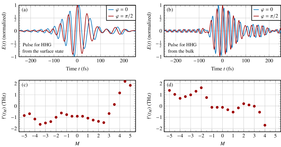
Figure 6: (a) and (b): Experimental pulse shapes from Ref. [10] that lead to HHG (a) from the topological surface state of Bi₂Te₃ and (b) from the bulk of Bi₂Te₃. (c) and (d): Time-local chirp ${\mathfrak{f}}^{\prime}(t^{(0)}_{M}(\varphi{=}\pi/2))$ evaluated from Eq. (24) for the pulse shapes from (a) and (b), respectively. At highest field, $M\hskip 1.52998pt{=}\hskip 1.52998pt0$, we have (c) ${\mathfrak{f}}^{\prime}(t^{(0)}_{0}(\varphi{=}\pi/2))\hskip 1.52998pt{=}\hskip 1.52998pt{-}\,1.0$ THz and (d) ${\mathfrak{f}}^{\prime}(t^{(0)}_{0}(\varphi{=}\pi/2))\hskip 1.52998pt{=}\hskip 1.52998pt{-}\,0.1$ THz.

Appendix F Parameters of the fits reported in Fig. 4

In Table 2, we report the full set of fit parameters obtained from the fitting in Fig. 4.

Appendix G Evaluating the time-local chirp of experimental electric field pulses

In this appendix, we evaluate the average chirp $\bar{\mathfrak{f}}^{\prime}$ [definition in Eq. (34)] for two electric field pulses that have been employed in the experiment by Schmid et al. [10] The experimental electric field pulses are sketched in Fig. 6 (a) and (b), where pulse (a) has been used for HHG from the topological surface state of Bi₂Te₃ and pulse (b) for HHG from the bulk of Bi₂Te₃ [10].

We evaluate the ”time-local chirp” ${\mathfrak{f}}^{\prime}(t^{(0)}_{M}(\varphi))$ which is the key quantity in our analytical formulae (17) and (18). ${\mathfrak{f}}^{\prime}(t^{(0)}_{M}(\varphi))$ follows from Eq. (24), ${\mathfrak{f}}^{\prime}(t^{(0)}_{M}(\varphi))\hskip 1.69998pt{=}\hskip 1.69998pt1\hskip 1.69998pt{-}\hskip 1.69998ptt_{m}(\varphi)/t^{(0)}_{m}(\varphi)$. The results for ${\mathfrak{f}}^{\prime}(t^{(0)}_{M}(\varphi))$ for the pulses in (a) and (b) with CEP $\varphi\hskip 1.69998pt{=}\hskip 1.69998pt\pi/2$ are sketched in Fig. 6 (c) and (d), respectively.

For the pulse from Fig. 6 (a), we observe that close to $M\hskip 1.69998pt{=}\hskip 1.69998pt0$, we have a constant time-local chirp ${\mathfrak{f}}^{\prime}\hskip 1.69998pt{\approx}\hskip 1.69998pt{-}\hskip 0.50003pt0.92$ THz (giving $-2\pi\bar{\mathfrak{f}}^{\prime}/\omega_{0}\hskip 1.69998pt{\approx}\hskip 1.69998pt0.037$ with $\omega_{0}\hskip 1.69998pt{=}\hskip 1.69998pt2\pi\hskip 1.69998pt{\cdot}\hskip 1.69998pt25$ THz) while for roots $|M|\hskip 1.69998pt{>}\hskip 1.69998pt1$, the time-local chirp varies. Thus, higher-order derivatives of ${\mathfrak{f}}$ become important that are not included in the analysis in App. C and in our analytical result (17).

For the pulse from Fig. 6 (b), we calculate an average time-local chirp $\bar{\mathfrak{f}}^{\prime}\hskip 1.69998pt{=}\hskip 1.69998pt0.29$ THz (average taken in the time interval $[-40\,\text{fs},50\,\text{fs}]$). With the frequency $\omega_{0}\hskip 1.69998pt{=}\hskip 1.69998pt2\pi\hskip 1.69998pt{\cdot}\hskip 1.69998pt42$ THz, we have $-2\pi\bar{\mathfrak{f}}^{\prime}/\omega_{0}\hskip 1.69998pt{=}\hskip 1.69998pt0.0069$ for the pulse from Fig. 6 (b).

Please note, that, compared to the data in Ref. 10, we have redefined the CEP, $-\,\varphi\hskip 1.49994pt{\rightarrow}\hskip 1.49994pt\varphi\hskip 1.69998pt{+}\hskip 1.69998pt2\pi$, to match the definition in Ref. [10] to the definition in our work.

Appendix H Verification of the analytical CEP-shift formula for various pulse shapes and Hamiltonians

In the main text, we have reported high-harmonics spectra for a time-dependent electric field $E(t)$, Eq. (4), with amplitude $E_{0}\hskip 1.69998pt{=}\hskip 1.69998pt3\,\mathrm{MV/cm}$, frequency $\omega\hskip 1.69998pt{=}\hskip 1.69998pt2\pi\cdot 25\,$THz, and pulse duration $\sigma\hskip 1.69998pt{=}\hskip 1.69998pt90\,\mathrm{fs}$. We also kept the dephasing time $T_{2}\hskip 1.69998pt{=}\hskip 1.69998pt10\,\mathrm{fs}$ and the Bi₂Te₃ surface-state Hamiltonian [10] unchanged in all simulations in the main text. In the main text, we only varied the CEP $\varphi$ and the chirp $f_{\text{chirp}}$. In this appendix, we show high-harmonics spectra for more values of $f_{\text{chirp}}$, $\sigma$, $E_{0}$, $\omega$, $T_{2}$ and for additional Hamiltonians.

First, we show the extrema of the emission spectrum for chirp $f_{\text{chirp}}\hskip 1.69998pt{=}\hskip 1.69998pt{-}\,2.5$ THz, $f_{\text{chirp}}\hskip 1.69998pt{=}\hskip 1.69998pt0$, and $f_{\text{chirp}}\hskip 1.69998pt{=}\hskip 1.69998pt1.25$ THz in Fig. 7 (a) – (c). We observe that the tilt angle $d\varphi/d\omega$ for chirp $f_{\text{chirp}}\hskip 1.69998pt{=}\hskip 1.69998pt{-}\,2.5$ THz [Fig. 7 (a)] is roughly doubled compared to $f_{\text{chirp}}\hskip 1.69998pt{=}\hskip 1.69998pt{-}\,1.25$ THz (Fig. 2), fully in line with our analytical formula (17). For a chirp $f_{\text{chirp}}\hskip 1.69998pt{=}\hskip 1.69998pt{+}\,1.25$ THz [Fig. 7 (c)], the tilt angle $d\varphi/d\omega$ changes its sign, i.e. the extremal lines are tilted to the left (from north west to sourth east), as predicted by our analytical formula (17). For chirp $f_{\text{chirp}}\hskip 1.69998pt{=}\hskip 1.69998pt0$, our analytical formula (17) predicts a vanishing tilt angle $d\varphi/d\omega$. This prediction is in line with the simulation reported in Fig. 7 (b) for $f_{\text{chirp}}\hskip 1.69998pt{=}\hskip 1.69998pt0$, where we observe a tilt angle $d\varphi/d\omega$ that is much reduced compared to $f_{\text{chirp}}\hskip 1.69998pt{=}\hskip 1.69998pt{-}\,2.5$ THz and $f_{\text{chirp}}\hskip 1.69998pt{=}\hskip 1.69998pt1.25$ THz [Fig. 7 (a) and (c)].

We next consider a short pulse with a duration $\sigma\hskip 1.69998pt{=}\hskip 1.69998pt50$ fs that has approximately only a single cycle $\sigma\omega/(2\pi)\hskip 1.69998pt{=}\hskip 1.69998pt1.25$ (with $\omega\hskip 1.69998pt{=}\hskip 1.69998pt2\pi\hskip 1.69998pt{\cdot}\hskip 1.69998pt25\,$THz). Moreover, we choose a vanishing chirp $f_{\text{chirp}}\hskip 1.69998pt{=}\hskip 1.69998pt0$, thus our analytical formula predicts a vanishing tilt angle. We report the extrema of the emission spectrum in Fig. 7 (d). For harmonics up to 20th order, we observe a small tilt angle $d\omega/d\varphi$, that increases with $\omega$. We observe that irregular patterns arise above 20th harmonic order with positive and negative tilts $d\omega/d\varphi$. This pattern hints to another mechanism underlying the CEP shifts which is not related to the chirp of the pulse, that is zero. Such mechanisms have already been suggested [11].

We continue to discuss the extrema in HHG for a short pulse $\sigma\hskip 1.69998pt{=}\hskip 1.69998pt50\,\text{fs}$ with chirp $f_{\text{chirp}}\hskip 1.69998pt{=}\hskip 1.69998pt{\pm}1.25$ THz. The corresponding extrema in the HHG spectra are shown in Fig. 8 (a) and (b). We observe that, the tilt $d\omega/d\varphi$ is to the right for $f_{\text{chirp}}\hskip 1.69998pt{=}\hskip 1.69998pt{-}1.25$ THz in Fig. 8 (a), in line with the analytical formula (17). In contract, no preferred tilt direction is observed for $f_{\text{chirp}}\hskip 1.69998pt{=}\hskip 1.69998pt{+}1.25$ THz in Fig. 8 (b), which is in contrast to our analytical formula (17). We speculate that an additional mechanism for generating CEP shifts are present for such a short pulse with only $\sigma\omega/(2\pi)\hskip 1.69998pt{=}\hskip 1.69998pt1.25$ cycles, limiting the predictive accuracy of our analytical formula (17) to many-cycle pulses with $\sigma\omega/(2\pi)\hskip 1.69998pt{\gg}\hskip 1.69998pt1$. For very long pulses with $\sigma\hskip 1.69998pt{=}\hskip 1.69998pt200$ fs, we find tilts $d\omega/d\varphi$ to the right for $f_{\text{chirp}}\hskip 1.69998pt{=}\hskip 1.69998pt{-}1.25$ THz [Fig. 8 (c)] and tilts to the left for $f_{\text{chirp}}\hskip 1.69998pt{=}\hskip 1.69998pt{+}1.25$ THz [Fig. 8 (d)]

Furthermore, we report CEP-dependent high-harmonic spectra $I(\omega)$ for other parameters in the SBE simulations: $T_{2}\hskip 1.49994pt{\in}\hskip 1.49994pt\{1\,\text{fs},\,100\,\mathrm{fs}\}$ in Fig. 9, field strength $E_{0}\hskip 1.49994pt{\in}\hskip 1.49994pt\{0.1\,\text{MV/cm},30\,\mathrm{MV/cm}\}$ in Fig. 10, and in addition, semiconducting Hamiltonians in Fig. 11. We observe in Figs. 9 and 10 that the tilt angle $d\omega/d\varphi$ increases with increasing harmonic order and that the tilt angle is reversed when changing the sign of the chirp. Both observations are fully in line with our analytical formula (17).

We calculate the high-harmonic spectrum from two semiconductor models in Fig. 11 (d)-(f) and (g)-(i), in comparison to a model for the topological surface state, Fig. 11 (a)-(c). The model underlying Fig. 11 (d)-(f) is the bulk semiconductor model for Bi₂Te₃ from Ref. [10]; the semiconductor model underlying Fig. 11 (g)-(i) is one-dimensional and has constant dipole and symmetric cosine-like bands. We choose a very short dephasing time for the bulk systems, $T_{2}\hskip 1.69998pt{=}\hskip 1.69998pt1$ fs, and very short damping time of band occupations towards the ground state, $T_{1}\hskip 1.69998pt{=}\hskip 1.69998pt10$ fs.  For semiconductors, we choose the same pulse shape as it has been used for modeling the semiconducting bulk of Bi₂Te₃ in Ref. [10]. For all three Hamiltonians, we observe similar tilt angles, for negative chirp to the right [Fig. 11 (a), (d), (g)], for positive chirp to the left [Fig. 11 (c), (f), (i)], and for zero chirp almost no tilt [Fig. 11 (b), (e), (h)], in line with our analytical formula (17).

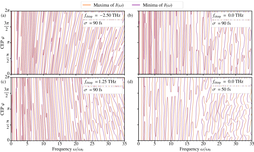
Figure 7: Local extrema of $I(\omega)$ computed from SBEs for the Bi₂Te₃-surface-state Hamiltonian as in Fig. 2 (b) but with varying pulse duration and with varying chirp in the driving electric field (4): (a) $f_{\text{chirp}}\hskip 1.52998pt{=}\hskip 1.52998pt{-}2.5$ THz, $\sigma\hskip 1.52998pt{=}\hskip 1.52998pt$90 fs, (b) $f_{\text{chirp}}\hskip 1.52998pt{=}\hskip 1.52998pt0$, $\sigma\hskip 1.52998pt{=}\hskip 1.52998pt$90 fs, (c) $f_{\text{chirp}}\hskip 1.52998pt{=}\hskip 1.52998pt1.25$ THz, $\sigma\hskip 1.52998pt{=}\hskip 1.52998pt$90 fs, (d) $f_{\text{chirp}}\hskip 1.52998pt{=}\hskip 1.52998pt0$, $\sigma\hskip 1.52998pt{=}\hskip 1.52998pt$50 fs,

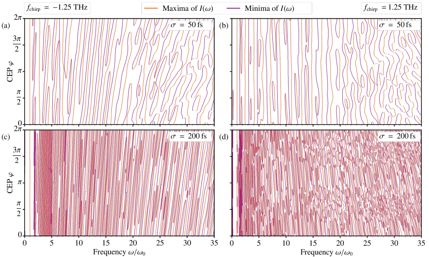
Figure 8: Local extrema of $I(\omega)$ computed from SBEs for the Bi₂Te₃-surface-state Hamiltonian as in Fig. 2 (b) but with varying pulse duration (a), (b) $\sigma\hskip 1.52998pt{=}\hskip 1.52998pt50\,\mathrm{fs}$ and (c), (d) $\sigma\hskip 1.52998pt{=}\hskip 1.52998pt200\,\mathrm{fs}$ (in Fig. 2 (b): $\sigma\hskip 1.52998pt{=}\hskip 1.52998pt90$ fs). For (a) and (c), we choose the shape of ${\bf E}(t)$ [Eq. (4)] as in Fig. 2 (b), in particular $f_{\text{chirp}}\hskip 1.52998pt{=}\hskip 1.52998pt-1.25$ THz. For (b) and (d), we choose $f_{\text{chirp}}\hskip 1.52998pt{=}\hskip 1.52998pt1.25$ THz which leads to an inversion of the tilt angle, fully in line with our analytical formula Eq. (17).

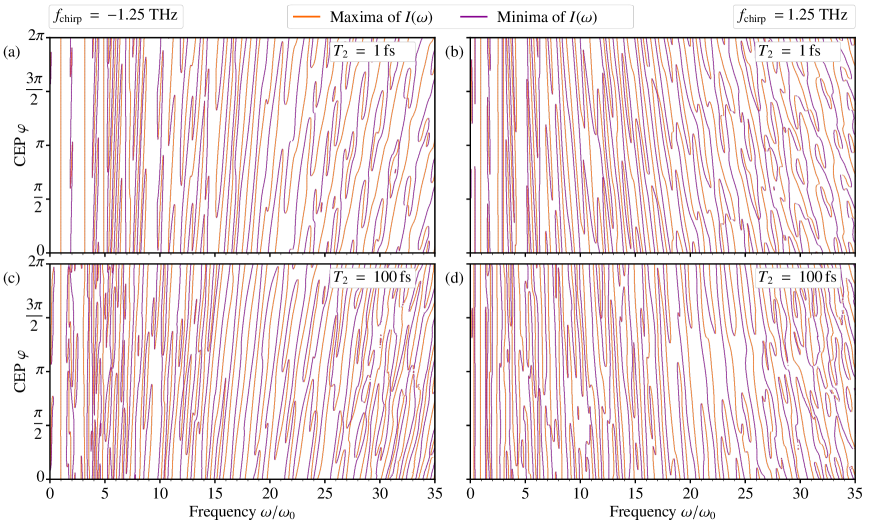
Figure 9: Local extrema of $I(\omega)$ computed from SBEs for the Bi₂Te₃-surface-state Hamiltonian as in Fig. 2 (b), but with a varying dephasing time of (a), (b) $T_{2}\hskip 1.52998pt{=}\hskip 1.52998pt1$ fs and (c), (d) $T_{2}\hskip 1.52998pt{=}\hskip 1.52998pt100$ fs (dephasing time in Fig. 2 (b): $T_{2}\hskip 1.52998pt{=}\hskip 1.52998pt10$ fs). For (a) and (c), we choose the driving field ${\bf E}(t)$ [Eq. (4)] as in Fig. 2 (b), in particular $f_{\text{chirp}}\hskip 1.52998pt{=}\hskip 1.52998pt-1.25$ THz. For (b) and (d), we choose $f_{\text{chirp}}\hskip 1.52998pt{=}\hskip 1.52998pt1.25$ THz which leads to an inversion of the tilt angle, fully in line with our analytical formula Eq. (17).

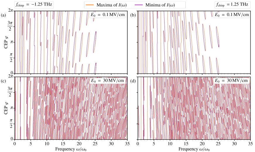
Figure 10: Local extrema of $I(\omega)$ computed from SBEs for the Bi₂Te₃-surface-state Hamiltonian as in Fig. 2 (b) but with varying driving field amplitude (a), (b) $E_{0}\hskip 1.52998pt{=}\hskip 1.52998pt0.1\,\mathrm{MV/cm}$ and (c), (d) $E_{0}\hskip 1.52998pt{=}\hskip 1.52998pt30\,\mathrm{MV/cm}$ (in Fig. 2 (b): $E_{0}\hskip 1.52998pt{=}\hskip 1.52998pt3$ MV/cm). For (a) and (c), we choose the shape of ${\bf E}(t)$ [Eq. (4)] as in Fig. 2 (b), in particular $f_{\text{chirp}}\hskip 1.52998pt{=}\hskip 1.52998pt-1.25$ THz. For (b) and (d), we choose $f_{\text{chirp}}\hskip 1.52998pt{=}\hskip 1.52998pt1.25$ THz which leads to an inversion of the tilt angle, fully in line with our analytical formula Eq. (17). We show extremal lines in (a) and (b) only up to harmonic order $\omega/\omega_{0}\hskip 1.52998pt{=}\hskip 1.52998pt26$ due to numerical noise present in higher harmonic orders.

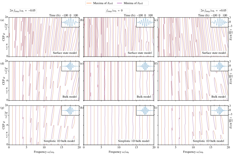
Figure 11: Local extrema of $I(\omega)$ computed from SBE’s for the topological surface state (a,b,c) as in Fig. 2, the Bulk Hamiltonian of Bi₂Te₃ (d,e,f) from Ref. [10] and a one dimensional model with constant dipole and symmetric cosine-like bands (g,h,i). For the latter, we use a gap of 0.15 eV and a band width of 8.7 eV. The Brillouin zone has a size $2\pi/3\AA$ and dipole is $d\hskip 1.52998pt{=}\hskip 1.52998pt3e\AA$ (e: electric charge). We use three different chirp-frequency-ratios, (a,d,g) $2\pi\,f_{\text{chirp}}/\omega_{0}\hskip 1.52998pt{=}\hskip 1.52998pt{-}0.05$, (b,e,h) $f_{\text{chirp}}/\omega_{0}\hskip 1.52998pt{=}\hskip 1.52998pt0$ and (c,f,i) $2\pi\,f_{\text{chirp}}/\omega_{0}\hskip 1.52998pt{=}\hskip 1.52998pt{+}0.05$. For (a) - (c), the driving pulse is parametrized from Eq. (4) with $E_{0}\hskip 1.52998pt{=}\hskip 1.52998pt3\,\mathrm{MV/cm}$, $\omega_{0}\hskip 1.52998pt{=}\hskip 1.52998pt2\pi\hskip 1.52998pt{\cdot}\hskip 1.52998pt25\,\mathrm{THz}$ and $\sigma\hskip 1.52998pt{=}\hskip 1.52998pt90\,\mathrm{fs}$, as already used in Fig. 2. For (d) - (i), the parameters are $E_{0}\hskip 1.52998pt{=}\hskip 1.52998pt3\,\mathrm{MV/cm}$, $\omega_{0}\hskip 1.52998pt{=}\hskip 1.52998pt2\pi\hskip 1.52998pt{\cdot}\hskip 1.52998pt40\,\mathrm{THz}$ and $\sigma\hskip 1.52998pt{=}\hskip 1.52998pt50\,\mathrm{fs}$ as in Ref. [10] for simulating HHG from the semiconducting bulk of Bi₂Te₃. The respective electric fields for CEP $\varphi\hskip 1.52998pt{=}\hskip 1.52998pt0$ are shown in the insets. We employ a dephasing time $T_{2}\hskip 1.52998pt{=}\hskip 1.52998pt10$ fs for the surface state model [(a - c)] and $T_{2}\hskip 1.52998pt{=}\hskip 1.52998pt1$ fs in the bulk case [(d - i)] as in Ref. [10]. Additionally, the band occupations are damped towards the ground state with a damping time $T_{1}\hskip 1.52998pt{=}\hskip 1.52998pt10$ fs [only for (d) - (i)] as in Ref. [10].

References

- Chin et al. [2001] A. H. Chin, O. G. Calderón, and J. Kono, Extreme Midinfrared Nonlinear Optics in Semiconductors, Phys. Rev. Lett. 86, 3292 (2001).
- Ghimire et al. [2011] S. Ghimire, A. D. DiChiara, E. Sistrunk, P. Agostini, L. F. DiMauro, and D. A. Reis, Observation of high-order harmonic generation in a bulk crystal, Nat. Phys. 7, 138 (2011).
- Schubert et al. [2014] O. Schubert, M. Hohenleutner, F. Langer, B. Urbanek, C. Lange, U. Huttner, D. Golde, T. Meier, M. Kira, S. W. Koch, and R. Huber, Sub-cycle control of terahertz high-harmonic generation by dynamical Bloch oscillations, Nat. Photonics 8, 119 (2014).
- Hohenleutner et al. [2015] M. Hohenleutner, F. Langer, O. Schubert, M. Knorr, U. Huttner, S. W. Koch, M. Kira, and R. Huber, Real-time observation of interfering crystal electrons in high-harmonic generation, Nature 523, 572 (2015).
- Vampa et al. [2015a] G. Vampa, T. Hammond, N. Thiré, B. Schmidt, F. Légaré, C. McDonald, T. Brabec, and P. Corkum, Linking high harmonics from gases and solids, Nature 522, 462 (2015a).
- Luu et al. [2015] T. T. Luu, M. Garg, S. Y. Kruchinin, A. Moulet, M. T. Hassan, and E. Goulielmakis, Extreme ultraviolet high-harmonic spectroscopy of solids, Nature 521, 498 (2015).
- Garg et al. [2016] M. Garg, M. Zhan, T. T. Luu, H. Lakhotia, T. Klostermann, A. Guggenmos, and E. Goulielmakis, Multi-petahertz electronic metrology, Nature 538, 359 (2016).
- Yoshikawa et al. [2017] N. Yoshikawa, T. Tamaya, and K. Tanaka, High-harmonic generation in graphene enhanced by elliptically polarized light excitation, Science 356, 736 (2017).
- Hafez et al. [2018] H. A. Hafez, S. Kovalev, J.-C. Deinert, Z. Mics, B. Green, N. Awari, M. Chen, S. Germanskiy, U. Lehnert, J. Teichert, Z. Wang, K.-J. Tielrooij, Z. Liu, Z. Chen, A. Narita, K. Müllen, M. Bonn, M. Gensch, and D. Turchinovich, Extremely efficient terahertz high-harmonic generation in graphene by hot Dirac fermions, Nature 561, 507 (2018).
- Schmid et al. [2021] C. P. Schmid, L. Weigl, P. Grössing, V. Junk, C. Gorini, S. Schlauderer, S. Ito, M. Meierhofer, N. Hofmann, D. Afanasiev, J. Crewse, K. A. Kokh, O. E. Tereshchenko, J. Güdde, F. Evers, J. Wilhelm, K. Richter, U. Höfer, and R. Huber, Tunable non-integer high-harmonic generation in a topological insulator, Nature 593, 385 (2021).
- You et al. [2017] Y. S. You, M. Wu, Y. Yin, A. Chew, X. Ren, S. Gholam-Mirzaei, D. A. Browne, M. Chini, Z. Chang, K. J. Schafer, M. B. Gaarde, and S. Ghimire, Laser waveform control of extreme ultraviolet high harmonics from solids, Opt. Lett. 42, 1816 (2017).
- Sivis et al. [2017] M. Sivis, M. Taucer, G. Vampa, K. Johnston, A. Staudte, A. Y. Naumov, D. M. Villeneuve, C. Ropers, and P. B. Corkum, Tailored semiconductors for high-harmonic optoelectronics, Science 357, 303 (2017).
- Garg et al. [2018] M. Garg, H. Y. Kim, and E. Goulielmakis, Ultimate waveform reproducibility of extreme-ultraviolet pulses by high-harmonic generation in quartz, Nat. Photonics 12, 291 (2018).
- Vampa et al. [2015b] G. Vampa, T. J. Hammond, N. Thiré, B. E. Schmidt, F. Légaré, C. R. McDonald, T. Brabec, D. D. Klug, and P. B. Corkum, All-Optical Reconstruction of Crystal Band Structure, Phys. Rev. Lett. 115, 193603 (2015b).
- Tancogne-Dejean et al. [2017] N. Tancogne-Dejean, O. D. Mücke, F. X. Kärtner, and A. Rubio, Ellipticity dependence of high-harmonic generation in solids originating from coupled intraband and interband dynamics, Nat. Commun. 8, 745 (2017).
- Yue and Gaarde [2022] L. Yue and M. B. Gaarde, Introduction to theory of high-harmonic generation in solids: tutorial, J. Opt. Soc. Am. B 39, 535 (2022).
- Park et al. [2022] J. Park, A. Subramani, S. Kim, and M. F. Ciappina, Recent trends in high-order harmonic generation in solids, Adv. Phys.: X 7, 2003244 (2022).
- Luu and Wörner [2018] T. T. Luu and H. J. Wörner, Measurement of the Berry curvature of solids using high-harmonic spectroscopy, Nat. Commun. 9, 916 (2018).
- Liu et al. [2017] H. Liu, Y. Li, Y. S. You, S. Ghimire, T. F. Heinz, and D. A. Reis, High-harmonic generation from an atomically thin semiconductor, Nat. Phys. 13, 262 (2017).
- Silva et al. [2019a] R. Silva, Á. Jiménez-Galán, B. Amorim, O. Smirnova, and M. Ivanov, Topological strong-field physics on sub-laser-cycle timescale, Nat. Photonics 13, 849 (2019a).
- Chacón et al. [2020] A. Chacón, D. Kim, W. Zhu, S. P. Kelly, A. Dauphin, E. Pisanty, A. S. Maxwell, A. Picón, M. F. Ciappina, D. E. Kim, C. Ticknor, A. Saxena, and M. Lewenstein, Circular dichroism in higher-order harmonic generation: Heralding topological phases and transitions in Chern insulators, Phys. Rev. B 102, 134115 (2020).
- Baykusheva et al. [2021a] D. Baykusheva, A. Chacón, D. Kim, D. E. Kim, D. A. Reis, and S. Ghimire, Strong-field physics in three-dimensional topological insulators, Phys. Rev. A 103, 023101 (2021a).
- Shirai et al. [2018] H. Shirai, F. Kumaki, Y. Nomura, and T. Fuji, High-harmonic generation in solids driven by subcycle midinfrared pulses from two-color filamentation, Opt. Lett. 43, 2094 (2018).
- Leblanc et al. [2020] A. Leblanc, P. Lassonde, G. Dalla-Barba, E. Cormier, H. Ibrahim, and F. Légaré, Characterizing the carrier-envelope phase stability of mid-infrared laser pulses by high harmonic generation in solids, Opt. Express 28, 17161 (2020).
- Song et al. [2019] X. Song, R. Zuo, S. Yang, P. Li, T. Meier, and W. Yang, Attosecond temporal confinement of interband excitation by intraband motion, Opt. Express 27, 2225 (2019).
- Hollinger et al. [2020] R. Hollinger, D. Hoff, P. Wustelt, S. Skruszewicz, Y. Zhang, H. Kang, D. Würzler, T. Jungnickel, M. Dumergue, A. Nayak, R. Flender, L. Haizer, M. Kurucz, B. Kiss, S. Kühn, E. Cormier, C. Spielmann, G. G. Paulus, P. Tzallas, and M. Kübel, Carrier-envelope-phase measurement of few-cycle mid-infrared laser pulses using high harmonic generation in ZnO, Opt. Express 28, 7314 (2020).
- Goulielmakis and Brabec [2022] E. Goulielmakis and T. Brabec, High harmonic generation in condensed matter, Nat. Photonics 16, 411 (2022).
- Borsch et al. [2020] M. Borsch, C. P. Schmid, L. Weigl, S. Schlauderer, N. Hofmann, C. Lange, J. T. Steiner, S. W. Koch, R. Huber, and M. Kira, Super-resolution lightwave tomography of electronic bands in quantum materials, Science 370, 1204 (2020).
- Bauer and Hansen [2018] D. Bauer and K. K. Hansen, High-Harmonic Generation in Solids with and without Topological Edge States, Phys. Rev. Lett. 120, 177401 (2018).
- Drüeke and Bauer [2019] H. Drüeke and D. Bauer, Robustness of topologically sensitive harmonic generation in laser-driven linear chains, Phys. Rev. A 99, 053402 (2019).
- Jürß and Bauer [2019] C. Jürß and D. Bauer, High-harmonic generation in Su-Schrieffer-Heeger chains, Phys. Rev. B 99, 195428 (2019).
- Jürß and Bauer [2020] C. Jürß and D. Bauer, Helicity flip of high-order harmonic photons in Haldane nanoribbons, Phys. Rev. A 102, 043105 (2020).
- Moos et al. [2020] D. Moos, C. Jürß, and D. Bauer, Intense-laser-driven electron dynamics and high-order harmonic generation in solids including topological effects, Phys. Rev. A 102, 053112 (2020).
- Baykusheva et al. [2021b] D. Baykusheva, A. Chacón, J. Lu, T. P. Bailey, J. A. Sobota, H. Soifer, P. S. Kirchmann, C. Rotundu, C. Uher, T. F. Heinz, D. A. Reis, and S. Ghimire, All-Optical Probe of Three-Dimensional Topological Insulators Based on High-Harmonic Generation by Circularly Polarized Laser Fields, Nano Lett. 21, 8970 (2021b).
- Lou et al. [2021] Z. Lou, Y. Zheng, C. Liu, Z. Zeng, R. Li, and Z. Xu, Controlling of the harmonic generation induced by the Berry curvature, Opt. Express 29, 37809 (2021).
- Bharti et al. [2022] A. Bharti, M. S. Mrudul, and G. Dixit, High-harmonic spectroscopy of light-driven nonlinear anisotropic anomalous Hall effect in a Weyl semimetal, Phys. Rev. B 105, 155140 (2022).
- Bai et al. [2021] Y. Bai, F. Fei, S. Wang, N. Li, X. Li, F. Song, R. Li, Z. Xu, and P. Liu, High-harmonic generation from topological surface states, Nat. Phys. 17, 311 (2021).
- Reimann et al. [2018] J. Reimann, S. Schlauderer, C. P. Schmid, F. Langer, S. Baierl, K. A. Kokh, O. E. Tereshchenko, A. Kimura, C. Lange, J. Güdde, U. Höfer, and R. Huber, Subcycle observation of lightwave-driven Dirac currents in a topological surface band, Nature 562, 396 (2018).
- Giorgianni et al. [2016] F. Giorgianni, E. Chiadroni, A. Rovere, M. Cestelli-Guidi, A. Perucchi, M. Bellaveglia, M. Castellano, D. Di Giovenale, G. Di Pirro, M. Ferrario, R. Pompili, C. Vaccarezza, F. Villa, A. Cianchi, A. Mostacci, M. Petrarca, M. Brahlek, N. Koirala, S. Oh, and S. Lupi, Strong nonlinear terahertz response induced by Dirac surface states in Bi2Se3 topological insulator, Nat. Commun. 7, 11421 (2016).
- Jones et al. [2000] D. J. Jones, S. A. Diddams, J. K. Ranka, A. Stentz, R. S. Windeler, J. L. Hall, and S. T. Cundiff, Carrier-Envelope Phase Control of Femtosecond Mode-Locked Lasers and Direct Optical Frequency Synthesis, Science 288, 635 (2000).
- Paulus et al. [2001] G. G. Paulus, F. Grasbon, H. Walther, P. Villoresi, M. Nisoli, S. Stagira, E. Priori, and S. De Silvestri, Absolute-phase phenomena in photoionization with few-cycle laser pulses, Nature 414, 182 (2001).
- Baltuška et al. [2002] A. Baltuška, T. Fuji, and T. Kobayashi, Controlling the carrier-envelope phase of ultrashort light pulses with optical parametric amplifiers, Phys. Rev. Lett. 88, 133901 (2002).
- Cundiff and Ye [2003] S. T. Cundiff and J. Ye, Colloquium: Femtosecond optical frequency combs, Rev. Mod. Phys. 75, 325 (2003).
- Baltuška et al. [2003] A. Baltuška, T. Udem, M. Uiberacker, M. Hentschel, E. Goulielmakis, C. Gohle, R. Holzwarth, V. S. Yakovlev, A. Scrinzi, T. W. Hänsch, and F. Krausz, Attosecond control of electronic processes by intense light fields, Nature 421, 611 (2003).
- Manzoni et al. [2010] C. Manzoni, M. Först, H. Ehrke, and A. Cavalleri, Single-shot detection and direct control of carrier phase drift of midinfrared pulses, Opt. Lett. 35, 757 (2010).
- Meierhofer et al. [2022] M. Meierhofer, S. Maier, D. Afanasiev, J. Freudenstein, C. P. Schmid, and R. Huber, Interferometric carrier-envelope phase stabilization for ultrashort pulses in the mid-infrared, arXiv preprints , arXiv:2207.10073 (2022).
- Schmitt-Rink et al. [1988] S. Schmitt-Rink, D. S. Chemla, and H. Haug, Nonequilibrium theory of the optical Stark effect and spectral hole burning in semiconductors, Phys. Rev. B 37, 941 (1988).
- Lindberg and Koch [1988] M. Lindberg and S. W. Koch, Effective Bloch equations for semiconductors, Phys. Rev. B 38, 3342 (1988).
- Aversa and Sipe [1995] C. Aversa and J. E. Sipe, Nonlinear optical susceptibilities of semiconductors: Results with a length-gauge analysis, Phys. Rev. B 52, 14636 (1995).
- Schäfer and Wegener [2002] W. Schäfer and M. Wegener, Semiconductor Optics and Transport Phenomena (Springer, Heidelberg, 2002).
- Haug and Jauho [2008] H. Haug and A.-P. Jauho, Quantum Kinetics in Transport and Optics of Semiconductors (Springer, Heidelberg, 2008).
- Haug and Koch [2009] H. Haug and S. W. Koch, Quantum theory of the optical and electronic properties of semiconductors (World Scientific Publishing Co., New York, 2009).
- Kira and Koch [2011] M. Kira and S. W. Koch, Semiconductor Quantum Optics (Cambridge University Press, New York, 2011).
- Földi [2017] P. Földi, Gauge invariance and interpretation of interband and intraband processes in high-order harmonic generation from bulk solids, Phys. Rev. B 96, 035112 (2017).
- Silva et al. [2019b] R. E. F. Silva, F. Martín, and M. Ivanov, High harmonic generation in crystals using maximally localized Wannier functions, Phys. Rev. B 100, 195201 (2019b).
- Li et al. [2019] J. Li, X. Zhang, S. Fu, Y. Feng, B. Hu, and H. Du, Phase invariance of the semiconductor Bloch equations, Phys. Rev. A 100, 043404 (2019).
- Yue and Gaarde [2020] L. Yue and M. B. Gaarde, Structure gauges and laser gauges for the semiconductor Bloch equations in high-order harmonic generation in solids, Phys. Rev. A 101, 053411 (2020).
- Thong et al. [2021] L. H. Thong, C. Ngo, H. T. Duc, X. Song, and T. Meier, Microscopic analysis of high harmonic generation in semiconductors with degenerate bands, Phys. Rev. B 103, 085201 (2021).
- Wilhelm et al. [2021] J. Wilhelm, P. Grössing, A. Seith, J. Crewse, M. Nitsch, L. Weigl, C. Schmid, and F. Evers, Semiconductor Bloch-equations formalism: Derivation and application to high-harmonic generation from Dirac fermions, Phys. Rev. B 103, 125419 (2021).
- Zhou et al. [1996] J. Zhou, J. Peatross, M. M. Murnane, H. C. Kapteyn, and I. P. Christov, Enhanced high-harmonic generation using 25 fs laser pulses, Phys. Rev. Lett. 76, 752 (1996).
- Shin et al. [1999] H. J. Shin, D. G. Lee, Y. H. Cha, K. H. Hong, and C. H. Nam, Generation of nonadiabatic blueshift of high harmonics in an intense femtosecond laser field, Phys. Rev. Lett. 83, 2544 (1999).
- Lee et al. [2001] D. G. Lee, J.-H. Kim, K.-H. Hong, and C. H. Nam, Coherent control of high-order harmonics with chirped femtosecond laser pulses, Phys. Rev. Lett. 87, 243902 (2001).
-
Note [1]
Other kinds of CEP shifts that also give useful
characterizations of the map can be conceived, too. For
example, rather than tracing lines with , one can trace maxima or minima, so
requiring , see Fig. 2\tmspace+.1667em(b) as an example. In analogy to Eq. (2\@@italiccorr), we then consider
which, together with the defining requirement , leads to an alternative set of lines in the - plane with tilt angle
This definition and definition (3\@@italiccorr) are equivalent in case maxima and minima lines are also equi-intensity lines. - Liu et al. [2010] C.-X. Liu, X.-L. Qi, H.-J. Zhang, X. Dai, Z. Fang, and S.-C. Zhang, Model Hamiltonian for topological insulators, Phys. Rev. B 82, 045122 (2010).
- Ashcroft and Mermin [1976] N. Ashcroft and N. Mermin, Solid State Physics (Saunders College, Philadelphia, 1976).
- Xiao et al. [2010] D. Xiao, M.-C. Chang, and Q. Niu, Berry phase effects on electronic properties, Rev. Mod. Phys. 82, 1959 (2010).
- Bloch [1929] F. Bloch, Über die Quantenmechanik der Elektronen in Kristallgittern, Z. Phys. 52, 555 (1929).
- Ghimire et al. [2012] S. Ghimire, A. D. DiChiara, E. Sistrunk, G. Ndabashimiye, U. B. Szafruga, A. Mohammad, P. Agostini, L. F. DiMauro, and D. A. Reis, Generation and propagation of high-order harmonics in crystals, Phys. Rev. A 85, 043836 (2012).
- Note [2] Note that due to the special nature of the Dirac-dispersion, the acceleration does not scale with the applied force . The electric field enters only indirectly in the sense that for non-vanishing a minimum field-strength is required to produce zeros in .
- Note [3] This conclusion has already been drawn in Refs. [11], [23] and [76, 77, 78, 79].
- Floss et al. [2018] I. Floss, C. Lemell, G. Wachter, V. Smejkal, S. A. Sato, X.-M. Tong, K. Yabana, and J. Burgdörfer, Ab initio multiscale simulation of high-order harmonic generation in solids, Phys. Rev. A 97, 011401(R) (2018).
- SciPy 1.0 Contributors [2020] SciPy 1.0 Contributors, SciPy 1.0: fundamental algorithms for scientific computing in Python, Nat. Methods 17, 261 (2020).
- Al-Naib et al. [2014] I. Al-Naib, J. E. Sipe, and M. M. Dignam, High harmonic generation in undoped graphene: Interplay of inter- and intraband dynamics, Phys. Rev. B 90, 245423 (2014).
- Monkhorst and Pack [1976] H. J. Monkhorst and J. D. Pack, Special points for Brillouin-zone integrations, Phys. Rev. B 13, 5188 (1976).
- Note [4] Scattering mechanisms are expected to be much more efficient in semiconductors and in the semiconducting bulk of topological insulators (Ref. [10]) compared to topological surface states with spin-momentum locking.
- Frolov et al. [2011] M. V. Frolov, N. L. Manakov, A. A. Silaev, N. V. Vvedenskii, and A. F. Starace, High-order harmonic generation by atoms in a few-cycle laser pulse: Carrier-envelope phase and many-electron effects, Phys. Rev. A 83, 021405(R) (2011).
- Frolov et al. [2012] M. V. Frolov, N. L. Manakov, A. M. Popov, O. V. Tikhonova, E. A. Volkova, A. A. Silaev, N. V. Vvedenskii, and A. F. Starace, Analytic theory of high-order-harmonic generation by an intense few-cycle laser pulse, Phys. Rev. A 85, 033416 (2012).
- Naumov et al. [2015] A. Y. Naumov, D. M. Villeneuve, and H. Niikura, Contribution of multiple electron trajectories to high-harmonic generation in the few-cycle regime, Phys. Rev. A 91, 063421 (2015).
- Sansone [2009] G. Sansone, Quantum path analysis of isolated attosecond pulse generation by polarization gating, Phys. Rev. A 79, 053410 (2009).