GANimator: Neural Motion Synthesis from a Single Sequence

Abstract.

We present GANimator, a generative model that learns to synthesize novel motions from a single, short motion sequence. GANimator generates motions that resemble the core elements of the original motion, while simultaneously synthesizing novel and diverse movements. Existing data-driven techniques for motion synthesis require a large motion dataset which contains the desired and specific skeletal structure. By contrast, GANimator only requires training on a single motion sequence, enabling novel motion synthesis for a variety of skeletal structures e.g., bipeds, quadropeds, hexapeds, and more. Our framework contains a series of generative and adversarial neural networks, each responsible for generating motions in a specific frame rate. The framework progressively learns to synthesize motion from random noise, enabling hierarchical control over the generated motion content across varying levels of detail. We show a number of applications, including crowd simulation, key-frame editing, style transfer, and interactive control, which all learn from a single input sequence. Code and data for this paper are at https://peizhuoli.github.io/ganimator.

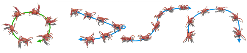
Figure 1. Given a single training motion sequence of skeleton with arbitrary topology, our method learns to []synthesize novel motion sequences.

1. Introduction

Generating realistic and diverse human motion is a long-standing objective in computer graphics. Motion modeling and synthesis commonly uses a probabilistic model to capture limited local variations (Li et al., 2002) or utilizes a large motion dataset obtained by motion capture (mocap) (Holden et al., 2016). Capturing data with a mocap system is costly both during stage-setting and in post-process (e.g., involving manual data clean-up). Motion datasets are often limited, i.e., they lack the desired skeletal structure, body proportions, or styles. Therefore, utilizing motion datasets often requires non-trivial processing such as retargeting, which may potentially degrade or introduce errors in the original captured motion. Moreover, there are no extensive datasets which contain imaginary creatures or non-standard animals (such as the hexapedal crab in Figure 1), which limits existing data-driven techniques.

In this work, we develop a framework that is capable of generating diverse and realistic motions using only a single training sequence. Our strategy greatly simplifies the data collection process while still allowing the framework to create realistic variations and faithfully capture the details of the individual motion sequence. Inspired by the SinGAN model for image synthesis (Shaham et al., 2019), our key idea is to leverage the information within a single motion sequence in order to exploit the rich data over multiple temporal and spatial scales. The generation process is divided into several levels, similar to progressive training schemes for images (Karras et al., 2018; Shaham et al., 2019).

Our framework is an effective tool for generating novel motion which is not exactly present in the single given training sequence. GANimator can synthesize long, diverse, and high-quality motion sequences using only a short motion sequence as input. We show that for various types of motions and characters, we generate sequences that still resemble the core elements of the original motion, while simultaneously synthesizing novel and diverse movements. It should be noted that the synthesized motion is not copied verbatim from the original sequence. Namely, patches from the original motion do not appear in the synthesized motion.

We demonstrate the utility of the GANimator framework to generate both conditional and unconditional motion sequences that are reminiscent of the input motion. GANimator can unconditionally (i.e., driven by noise) generate motions for simulating crowds and motion editing/mixing. In addition, GANimator is able to produce controllable motion sequences, which are conditioned on a user-given input (e.g., trajectory position). We are able to inject global position and rotation of the root joint as an input for interactively controlling the trajectory of the synthesized motion. GANimator is also able to perform key-frame editing, which generates high-quality interpolations between user-modified poses. Lastly, GANimator enables motion style transfer – synthesizing the style of the input motion onto a different motion.

Our system relies on skeleton-aware operators (Aberman et al., 2020a) as a backbone for our neural motion synthesis framework. The skeleton-aware layers provides the platform for applying convolutions over a fixed skeleton topology. Since our network trains on a single motion sequence, we automatically adjust the operators to adhere to the structure of the input skeleton. Therefore, our system is able to train on a wide variety of skeletal structures, e.g., bipeds, quadropeds, hexapeds, and more. Further, for ground-inhabiting creatures, we incorporate a self-supervised foot contact label. This ensures proper placement of the feet on the ground plane and avoids notorious foot sliding artifacts. We demonstrate the effectiveness of GANimator in handling a wide variety of skeletal structures and motions, and its applicability in various motion editing and synthesis tasks.

Achieving desirable results in this constrained scenario is highly challenging, with existing techniques commonly producing undesirable results that fall into one of two extremes. In the first extreme, generated results span the breadth of poses contained in the original motion sequence, but are jittery and incoherent. In the second extreme, results are smooth, but lack variety and coverage of the motion elements contained in the original sequence. Our proposed technique strikes a favorable balance between these extremes, synthesizing high-quality, novel, and varied motion sequences. Our framework produces desirable motion sequences that contain all the original motion elements, while still achieving diverse and smooth motion sequences.

2. Related Work

We review various relevant works on motion generation, focusing on human and other character animation. For an in-depth survey of this extensive body of literature we refer the readers to the surveys in (Geijtenbeek et al., 2011; Mourot et al., 2021).

Statistical modeling of visual and motion data.

Representing and generating complex visual objects and phenomena of stochastic nature, such as stone and wood textures or breathing and walking cycles with natural variations, is one of the fundamental tasks in computer graphics. In one of the pioneer works in this area, Perlin (1985) introduced the famous Perlin noise function that can be used for image synthesis with variations. This technique was later applied to procedural animation synthesis (Perlin and Goldberg, 1996) to achieve random variability. Instead of using additive noise, statistical approaches (Pullen and Bregler, 2000; Brand and Hertzmann, 2000; Bowden, 2000; Chai and Hodgins, 2007) propose using probabilistic models such as kernel-based distribution and hidden Markov models, enabling synthesis with variations via direct sampling of the model. To capture both local and global structure, MotionTexture (Li et al., 2002) clusters a large training dataset into textons, a linear dynamics model capable of capturing local variation, and models the transition probability between textons. Though the goal resembles ours, this data-hungry statistical model does not fit in our single-motion setting. We perform an in-depth comparison to MotionTexture regarding the ability to model both global and local variations when data is limited in Sec. 4.2. A similar idea of using two-level statistical models is employed in multiple works (Tanco and Hilton, 2000; Lee et al., 2002) for novel motion synthesis. Other statistical models based on Gaussian processes learn a compact latent space (Grochow et al., 2004; Wang et al., 2007; Levine et al., 2012) or facilitate an interactive authoring process (Ikemoto et al., 2009) from a small set of examples for multiple applications, including inverse kinematics, motion editing and task-guided character control. Lau et al. (2009) use a similar Bayesian approach to model the natural variation in human motion from several examples. However, probabilistic approaches tend to capture limited variations in local frames and require a large dataset for a better understanding of global structure variations.

Interpolation and blending of examples.

Another approach for example-based motion generation is explicit blending and concatenation of existing examples. Early works (Rose et al., 1996; Wiley and Hahn, 1997; Rose et al., 1998; Mizuguchi et al., 2001; Park et al., 2002) use various interpolation and warping techniques for this purpose. Matching-based works (Pullen and Bregler, 2002; Arikan and Forsyth, 2002; Kovar and Gleicher, 2004) generate motion by matching user-specified constraints in the existing dataset and interpolating the retrieved clips. Kovar et al. (2002) explicitly model the structure of a corpus of motion capture data using an automatically constructed directed graph (the motion graph). This approach enables flexible and controllable motion generation and is widely used in interactive applications like computer games. Min et al. (2012) propose a mixture of statistical and graph-based models to decouple variations in the global composition of motions or actions, and the local movement variations. One significant constraint of blending-based methods is that the diversity of the generated results is limited to the dataset, since it is composed of interpolations and combinations of the dataset. Further works (Heck and Gleicher, 2007; Safonova and Hodgins, 2007; Zhao et al., 2009) focus on the efficiency and robustness of the algorithm but are still inherently limited in the variety of the generated results. Motion matching (Büttner and Clavet, 2015) directly finds the best match in the mocap dataset given the user-provided constraints, bypassing the construction of a graph to achieve better realism. However, it generally requires task-specific tuning and is unable to generate novel motion that are unseen in the dataset.

Physics-based motion synthesis.

Another loosely related field is physically-based motion generation, where the generation process runs a controller in a physics simulator, unlike kinematics approaches that directly deal with joints’ transformations. Agrawal et al. (2013) optimize a procedural controller given a motion example to achieve physical plausibility while ensuring diversity in generated results. However, such controllers are hand-crafted for specific tasks, such as jumping and walking, and are thus difficult to generalize to different motion data. Results in (Ye and Liu, 2010; Wei et al., 2011) show that combining physical constraints and statistical priors helps generate physically realistic animations and reactions to external forces, but the richness of motion is still restricted to the learned prior. With the evolution of deep reinforcement learning, control policies on different bodies including biped locomotion (Heess et al., 2017; Peng et al., 2017) and quadurpeds (Luo et al., 2020) can be learned from scratch without reference. It is also possible to achieve high quality motion by learning from reference animation (Peng et al., 2018). Lee et al. (2021) propose to learn a parameterized family of control policies from a single clip of a single movement, e.g., jumping, kicking, backflipping, and are able to generate novel motions for a different environment, target task, and character parameterization. As in other works, the learned policy is limited to several predefined tasks.

Neural motion generation.

Taylor and Hinton (2009) made initial attempts to model motion style with neural networks by restricted Boltzmann machines. Holden et al. (2015; 2016) applied convolutional neural networks (CNN) to motion data for learning a motion manifold and motion editing. Concurrently, Fragkiadaki et al. (2015) chose to use recurrent neural networks (RNN) for motion modeling. RNN based works also succeed in short-term motion prediction (Fragkiadaki et al., 2015; Pavllo et al., 2018), interactive motion generation (Lee et al., 2018) and music-driven motion synthesis (Aristidou et al., 2021). Zhou et al. (2018) tackle the problem of error accumulation in long-term random generation by alternating the network’s output and ground truth as the input of RNN during training. This method, called acRNN, is able to generate long and stable motion similar to the training set. However, like many other deep learning based methods, it struggles when only a short training sequence is provided, whereas we are able to address the limited data problem. We compare our method to acRNN in Sec. 4.2. Holden et al. (2017) propose phase-functioned neural networks (PFNN) for locomotion generation and introduce phase to neural networks. Similar ideas are used in quadruped motion generation by Zhang et al. (2018). Starke et al. (2020) extend phase to local joints to cope with more complex motion generation. Henter et al. (2020) propose another generative model for motion based on normalizing flow. Neural networks succeed in a variety of motion generation tasks: motion retargeting (Villegas et al., 2018; Aberman et al., 2020a, 2019), motion style transfer (Aberman et al., 2020b; Mason et al., 2022), key-frame based motion generation (Harvey et al., 2020), motion matching (Holden et al., 2020) and animation layering (Starke et al., 2021). It is worth noting that the success of deep learning methods hinges upon large and comprehensive mocap datasets. However, acquiring a dataset involves costly capturing steps and nontrivial post-processing, as discussed in Section 1. In contrast, our method achieves comparable results by learning from a single input motion sequence.

3. Method

We propose a generative model that can learn from a single motion sequence. Our approach is inspired by recent works in the image domain that use progressive generation (Karras et al., 2018) and works that propose to train deep networks on a single example (Shocher et al., 2019; Shaham et al., 2019). We next describe the main building blocks of our hierarchical framework, motion representation, and the training procedure.

3.1. Motion representation

We represent a motion sequence by a temporal set of $T$ poses that consists of root joint displacements ${\bf O}\in\mathds{R}^{T\times 3}$ and joint rotations ${\bf R}\in\mathds{R}^{T\times JQ}$, where $J$ is the number of joints and $Q$ is the number of rotation features. The rotations are defined in the coordinate frame of their parent in the kinematic chain, and represented by the 6D rotation features ($Q=6$) proposed by Zhou et al. (2019), which yields the best result among other representations for our task (see ablation study in Section 4.4).

To mitigate common foot sliding artifacts, we incorporate foot contact labels in our representation. In particular, we concatenate to the feature axis $C\cdot T$ binary values ${\bf L}\in\{0,1\}^{T\times C}$, which correspond to the contact labels of the foot joints, $\mathcal{F}$, of the specific creature. For example, for humanoids, we use $\mathcal{F}=\{$left heel, left toe, right heel, right toe$\}$. For each joint $j\in\mathcal{F}$ and frame $t\in\{1,\ldots,T\}$, the $tj$-th label is calculated via

$${\bf L}^{tj}=\mathds{1}[\|\text{FK}_{\bf S}(\left[{\bf R},{\bf O}\right])^{tj}\|_{2}<\epsilon],$$

where $\|\text{FK}_{\bf S}(\left[{\bf R},{\bf O}\right])^{tj}\|_{2}$ denotes the magnitude of the velocity of joint $j$ in frame $t$ retrieved by a forward kinematics (FK) operator. FK applies the rotation and root joint displacements on the skeleton ${\bf S}$, and $\mathds{1}[V]$ is an indicator function that returns 1 if $V$ is true and $0$ otherwise.

To simplify the notation, we denote the metric space of the concatenated features by $\mathcal{M}_{T}\equiv\mathds{R}^{T\times(JQ+C+3)}$. In addition, we denote the input motion features by ${\bf T}\equiv[{\bf R},{\bf O},{\bf L}]\in\mathcal{M}_{T}$, and its correponding downsampled versions by ${\bf T}_{i}\in\mathcal{M}_{T_{i}}$.

3.2. Progressive motion synthesis architecture

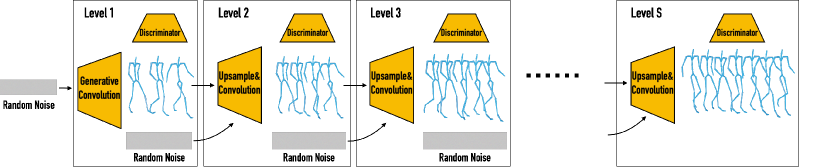
Figure 2. Our progressive motion synthesis architecture. Starting with random noise that synthesize a coarse motion sequence through a generative network, our framework progressively upsamples the motion until it reaches to the finest temporal resolution. Each level receives the output of the previous level (except for the first level) and a random noise as output an upsampled version of the input sequence. We use adversarial training, such that each generated result is fed into a discriminator at a corresponding level.

Our motion generation framework is illustrated in Fig 2. It consists of $S$ coarse-to-fine generative adversarial networks (GANs) (Goodfellow et al., 2014), each of which is responsible to generate motion sequences with a specific number of frames $\{T_{i}\}_{i=1}^{S}$. We denote the generators and discriminators by $\{G_{i}\}_{i=1}^{S}$ and $\{D_{i}\}_{i=1}^{S}$, respectively.

The first level is purely generative, namely, $G_{1}$ maps a random noise $z_{1}\in\mathcal{M}_{T_{1}}$ into a coarse motion sequence

(1) $${\bf Q}_{1}=G_{1}(z_{1}),$$

where ${\bf Q}_{1}\in\mathcal{M}_{T_{i}}$. Then, the generators in the finer levels $G_{i}$ $(2\leq i\leq S)$ progressively upsample ${\bf Q}_{1}$ via

(2) $${\bf Q}_{i}=G_{i}({\bf Q}_{i-1},z_{i}),$$

where in each level the sequence is upsampled by a fixed scaling factor $F>1$. The process is repeated until the finest output sequence ${\bf Q}_{S}\in\mathcal{M}_{T_{S}}$ is generated by $G_{S}$.

Note that $z_{i}\in\mathcal{M}_{T_{i}}$ has an i.i.d normal distribution $\sim\mathcal{N}\left(0,\sigma_{i}\right)$ along the temporal axis while being shared along the channel axis, and we found that $\sigma_{i}$ is highly correlated with the magnitude of the high-frequency details generated by $G_{i}$, thus, we select

(3) $$\sigma_{i}=\frac{1}{Z_{i}}\|\uparrow{\bf T}_{i-1}-{\bf T}_{i}\|_{2}^{2},$$

where $Z_{i}=T_{i}(QJ+C+3)$ is the number of entries in ${\bf T}_{i}$, and $\uparrow$ is a linear upsampler with a scaling factor $F>1$. In all of our experiments we select $F=4/3$ and $S=7$.

3.2.1. Network components

Generator

Our generator $G_{i}$ contains a fully convolutional neural network $g_{i}(\cdot)$ that has a few skeleton-aware convolution layers (Aberman et al., 2020a) followed by non-linear layers (see Appendix A). Since the main role of the network is to add missing high-frequency details, we use a residual structure (He et al., 2016), hence for $2\leq i\leq S$, we get

(4) $$G_{i}({\bf Q}_{i-1},z_{i})=g_{i}(\uparrow{\bf Q}_{i-1}+z_{i})+\uparrow{\bf Q}_{i-1}.$$

Discriminator.

While discriminators in classic GAN architectures output a single scalar indicating whether the input is classified as “real” or “fake”, such a structure in the case of a single sequence in the training data leads to mode collapse, since our generator trivially overfits the sequence. In order to prevent overfitting we limit the receptive field of the discriminator by employing a Patch-GAN (Isola et al., 2017; Li and Wand, 2016) classifier, which calculates a confidence value to each input patch. The final output of our discriminator is the average value of all the per-patch confidence values, predicted by the network.

Skeleton-aware operators.

We employ skeleton-aware convolutions (Aberman et al., 2020a) as a fundamental building block in our framework. Skeleton-aware operators require a fixed skeleton topology that is defined by a set of joints (vertices) and an adjacency list (edges). Since our network operates on a single sequence we adapt the topology to adhere the input sequence. This enables operation on any skeleton topology, and does not require retargeting the input motion to a specific skeletal structure. To incorporate the foot contact labels into the skeleton-aware representation, we treat each label as a virtual joint connected to its corresponding joint rotations vertex. In addition, due to the high correlation between end-effectors and global positions, we add a connection between the contact labels vertices to the vertex of the global displacements ${\bf O}$, where we treat the latter as another virtual joint that is connected to the neighbors of the root joint in the kinematic chain.

3.2.2. Loss functions

Adversarial Loss

We train level $i$ with the WGAN-GP (2017) loss:

$$\mathcal{L}_{\text{adv}} = \mathbb{E}_{{\bf Q}_{i}\sim\mathbb{P}_{g_{i}}}\left[D_{i}({\bf Q}_{i})\right]-D_{i}({\bf T}_{i})$$

$$+ \lambda_{\text{gp}}\mathbb{E}_{\hat{\bf Q}\sim\mathbb{P}_{\hat{g}_{i}}}\left[\left(\|\nabla D_{i}(\hat{\bf Q}_{i})\|_{2}-1\right)^{2}\right],$$

where $\mathbb{P}_{g_{i}}$ is defined as the distributions of our generated samples in the $i$th level, $\nabla$ is the gradient operator and $\mathbb{P}_{\hat{g}_{i}}$ is the distribution of the linear interpolations $\hat{\bf Q}_{i}=\lambda{\bf Q}_{i}+(1-\lambda){\bf T}_{i}$ with $\lambda$ as a uniformly distributed variable in $[0,1]$. The gradient penalty term in (3.2.2) enforces Lipschitz continuity so the Wasserstein distance between generated and training distribution can be well approximated (Gulrajani et al., 2017).

Reconstruction Loss

To ensure that the network generates variations of all the different temporal patches, and does not collapse to generation of a specific subset of movements, we require the network to reconstruct the input motion from a set of pre-defined noise signals $\{z_{i}^{*}\}_{i=1}^{S}$, namely, $G_{i}(\uparrow{\bf T}_{i-1},z_{i}^{*})$ should approximate the single training example ${\bf T}_{i}$ at level $i$. To encourage the system to do so, we define a reconstruction loss

(6) $$\mathcal{L}_{\text{rec}}=\|G_{i}(\uparrow{\bf T}_{i-1},z_{i}^{*})-{\bf T}_{i}\|_{1}.$$

Note that the noise models the variation of generated results, but during reconstruction, we do not expect any variation. To this end, we fix $z_{1}^{*}$ as a pre-generated noise for the first level and set $z_{i}^{*}=0$ for the other levels.

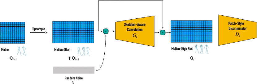
Figure 3. Generator structure. Our residual generator receives the sum of a noise vector and the upsampled result from previous level (in the first level it receives only noise). It predicts the missing high-frequency details, which is added to the input animation via skip connections.

Contact Consistency Loss

As accurate foot contact is one of the major factors of motion quality, we predict the foot contact labels in our framework and use an IK post-process to ensure the contact. Since the joint contact labels ${\bf L}$ are integrated into our motion representation $\mathcal{M}$, the skeleton-aware networks can directly operate on $\mathcal{M}$ and learn to predict the contact label as part of the motion.

We noticed that the implicit learning of contact labels can cause artifacts in the transition between activated and non-activated contact labels. Thus, we propose a new loss that encourages a consistency between contact label and feet velocity. We require that in every frame either the contact label or the foot velocity will be minimized, via

(7) $$\mathcal{L}_{\text{con}}=\frac{1}{T|\mathcal{F}|}\sum_{j\in\mathcal{F}}\sum_{t=1}^{T}\|\text{FK}_{\bf S}({\bf R},{\bf O})^{tj}\|_{2}^{2}\cdot s({\bf L}^{tj}),$$

where $s(x)=1/[1+\exp(5-10x)]$ is the transformed sigmoid function. We demonstrate the effectiveness of this loss in the ablation study (Section 4.4).

3.2.3. Training

Our full loss used for training summarizes as:

(8) $$\mathcal{L}=\lambda_{\text{adv}}\mathcal{L}_{\text{adv}}+\lambda_{\text{rec}}\mathcal{L}_{\text{rec}}+\lambda_{\text{con}}\mathcal{L}_{\text{con}}.$$

Although each level can be trained separately, the generated samples of generators in the low levels may be over-blurred due to low temporal resolution and the smoothing effect applied by convolutional kernel. To improve the robustness and quality of the results, we combine every 2 consecutive levels as a block and train the framework block by block. A similar technique is also used by Hinz et al. (2021).

For a detailed description of the layers in each component and the specific values of the hyper-parameters, we refer the reader to Appendix A.

4. Experiments and Evaluation

We evaluate our results, compare them to other motion generation techniques and demonstrate the effectiveness of various components in our framework through an ablation study. Please refer to the supplementary video for the qualitative evaluation.

4.1. Implementation details

Our GANimator framework is implemented in PyTorch (Paszke et al., 2019), and the experiments are performed on NVIDIA GeForce RTX 2080 Ti GPU. We optimize the parameters of our network with the loss term in Eq. (8) using the Adam optimizer (Kingma and Ba, 2014). We used different training sequences, whose length ranges from 140 frames to 800 frames at 30fps. It contains both artist-created animation and motion capture data from Mixamo (2021) and Truebones (2022). The training time is proportional to the training sequence length, e.g., it takes about 4 hours to train our network on a human animation sequence with around 600 frames (15,000 iterations per level).

4.2. Novel motion synthesis

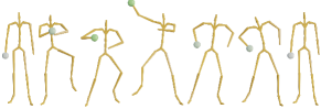
Training sequence

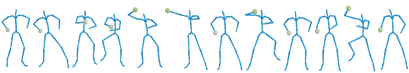
Ours

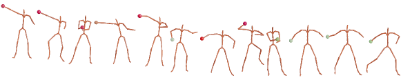
MotionTexture (2002)

acRNN (2018)

Figure 4. We train our framework, MotionTexture (2002) and acRNN (2018) on the Gangnam style dancing sequence with 371 frames and use them to synthesize a new sequence with 600 frames. The magnitude of velocity of the right hand is visualized with a heatmap (white - low, green - average, red - high). It can be seen that our method generates global structure variation, the poses and transitions look natural (see supplementary video) and visually similar to the training sequence. For MotionTexture (2002), we manually pick a path between all the trained textons to generate results with similar structure. However, it can be seen that such a process result in unnatural transitions visualized by the large hand velocity and bad foot contact. The result of acRNN (2018) converges to a static pose very quickly due to insufficient data and thus the velocity of the hand gradually vanishes.

We demonstrate the ability of motion sequence extrapolation in Fig. 4 and compare our method to the recent acRNN work (Zhou et al., 2018) and the classical statistical model MotionTexture (Li et al., 2002). We quantitatively compare these methods with metrics dedicated to a single training example in Section 4.3.

Since our network is fully convolutional, we can generate high-quality motion sequences of arbitrary length given a single training example. As a simple application, we can easily generate a crowd animation, as shown in Fig. 5 and the accompanying video.

When only a single training sequence is provided, acRNN can only generate a limited number of frames before converging to a constant pose, because the lack of data leads to an overfitted model that is not robust to perturbation and error accumulation in RNNs, while our fully convolutional framework does not suffer from this issue.

MotionTexture (Li et al., 2002) automatically clusters the patches of the training dataset into several textons and models the transition probability between textons, where each texton represents the variation of a small segment of similar motions. MotionTexture relies on similar but not identical patches in the dataset for modeling local variations. It constructs the global transition probability between textons based on the frequencies of consecutive relationships of corresponding patches in the dataset. However, when only a single training sequence is provided, we need to manually divide the sequence into patches and specify the transition between textons. When splitting the training sequences into several textons and manually permuting them to create global structure variations, the transitions between textons can be unnatural (see Fig. 4). It is possible to learn a single texton for the whole training sequence to achieve better quality, but the model creates almost zero local variations due to limited data.

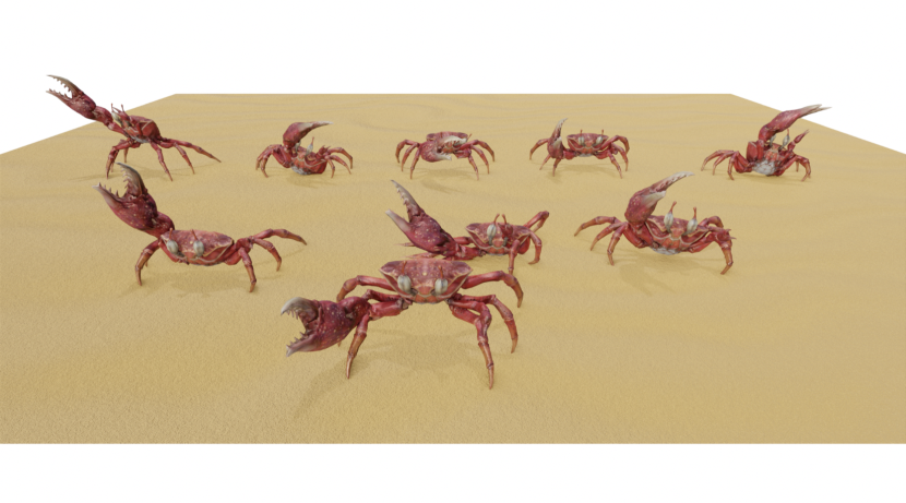
Figure 5. Crowd animation. Our framework trained on a single crab dancing sequence can synthesize various novel motions that can be used to simulate crowd and augment data for various purposes.

4.3. Evaluation

We discuss quantitative metrics for novel motion synthesis from a single training sequence and compare our method and existing motion generation techniques.

Coverage.

An important quantitative measurement for the quality of our model is the coverage of the training example. Since there is only one training example, we measure the coverage on all possible temporal windows $\mathcal{W}({\bf T},L)=\left\{{\bf T}^{i\,:\,i+L-1}\right\}_{i=1}^{L_{T}-L+1}$ of a given length $L$, where ${\bf T}^{i\,:\,j}$ denotes the sequence of frames $i$ to $j$ of the training example ${\bf T}$, and $L_{T}$ is the total length of ${\bf T}$. Given a generated result ${\bf Q}$, we label a temporal window ${\bf T}_{w}\in\mathcal{W}({\bf T},L_{c})$ as covered if its distance measure to the nearest neighbor in ${\bf Q}$ is smaller than an empirically chosen threshold $\epsilon$. The coverage of animation ${\bf Q}$ on ${\bf T}$ is defined as

(9) $$\text{Cov}({\bf Q},{\bf T})=\frac{1}{|\mathcal{W}({\bf T},L_{c})|}\sum_{{\bf T}_{w}\in\mathcal{W}({\bf T},L_{c})}\mathds{1}\left[\text{NN}({\bf T}_{w},{\bf Q})<\epsilon\right].$$

$\text{NN}({\bf Q}_{1},{\bf Q}_{2})$ denotes the distance of the nearest neighbor of the animation sequence ${\bf Q}_{1}$ in ${\bf Q}_{2}$. It is crucial to use an appropriate distance measure here. In our setting, we choose the Frobenius norm on the local joint rotation matrices:

(10) $$\text{NN}({\bf Q}_{1},{\bf Q}_{2})=\frac{1}{L_{1}}\min_{{\bf Q}_{w}\in\mathcal{W}({\bf Q}_{2},L_{1})}\left\|{\bf Q}_{1}-{\bf Q}_{w}\right\|_{F}^{2},$$

where $L_{1}$ is the length of ${\bf Q}_{1}$. We use joint rotations and not positions since our model creates local variations so that location deviations accumulate along the kinematics chain, which would cause location-based high distance measures on visually similar patches.

We choose $L_{c}=30$, capturing local patch length of 1 second. Similarly, the coverage of a model $\mathcal{G}(\cdot)$ on ${\bf T}$ is defined by

(11) $$\text{Cov}(\mathcal{G},{\bf T})=\mathbb{E}_{z}\text{Cov}(\mathcal{G}(z),{\bf T}).$$

Global diversity.

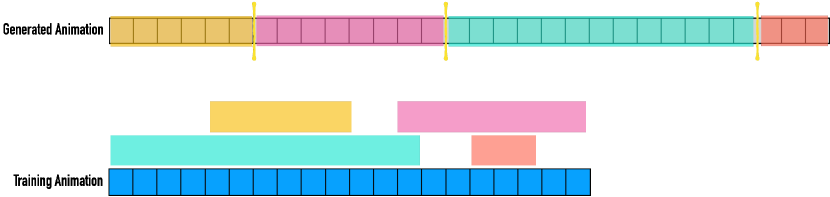
Figure 6. Patched Nearest Neighbor metric. The generated animation (top row) is divided into several segments, where the length of each segment is at least $T_{\min}$. Then each segment is assigned to its nearest neighbor in the training animation (bottom row) as visualised by the color bars.

To quantitatively measure the global structure diversity against a single training example, we propose to measure the distance between patched nearest neighbors (PNN). The idea is to divide the generated animation into several segments, where each segment is no shorter than a threshold $T_{\min}$, and find a segmentation that minimizes the average per-frame nearest neighbor cost as illustrated in Figure 6. For each frame $i$ in the generated animation ${\bf Q}$ we match it with frame $l_{i}$ in the training animation ${\bf T}$, such that between every neighboring points in the set of discontinuous points $\{i\ |\ l_{i}\neq l_{i-1}+1\}$ is at least $T_{\min}.$ This is because every discontinuous point corresponds to the starting point of a new segment. We call such an assignment $\{l_{i}\}_{i=1}^{L}$ a segmentation on ${\bf Q}.$ When large global structure variation is present, it is difficult to find a close nearest neighbor for large $T_{\min}$. The patched nearest neighbor is defined by, minimizing over all possible segmentations,

(12) $$\mathcal{L}_{\text{PNN}}=\min_{\{l_{i}\}}\frac{1}{L}\sum_{i=1}^{L}\|{\bf Q}^{i}-{\bf T}^{l_{i}}\|_{F}^{2},$$

where ${\bf Q}^{i}$ denotes frame $i$ in $Q$ and ${\bf T}^{l_{i}}$ denotes frame $l_{i}$ in ${\bf T}$. The PNN can be solved efficiently with dynamic programming, similar to MotionTexture (2002); we refer the reader to Appendix B for more details. In all our experiments, we choose $T_{\min}=30$, corresponding to one second of the animation.

Local diversity.

Our framework synthesizes animations carrying similar but diverse visual content compared to the training sequence. We measure the local frame diversity by comparing every local window ${\bf Q}_{w}\in\mathcal{W}({\bf Q},L_{d})$ of length $L_{d}$ to its nearest neighbor in the training sequence ${\bf T}$:

(13) $$\mathcal{L}_{\text{local}}=\frac{1}{|\mathcal{W}({\bf Q},L_{d})|}\sum_{{\bf Q}_{w}\in\mathcal{W}({\bf Q},L_{d})}\text{NN}({\bf Q}_{w},{\bf T}).$$

Similar to the definition of coverage, we use the Frobenius norm over local joint rotation matrices. We choose $L_{d}=15$ to capture local differences between the generated result and the training example.

We quantitatively compare our results to MotionTexture (Li et al., 2002) and acRNN (Zhou et al., 2018) using the metrics above as reported in Table 1. Since we use the nearest neighbor cost against the training sequence to measure diversity, high diversity score does not necessarily imply plausible results: MotionTexture creates unnatural transitions that are not part of the training sequence, and acRNN converges to a pose that does not exist in the training sequence also leading to a high diversity score. It can be seen that acRNN has limited coverage due to its convergence to a static pose, while our method generates motions that cover the training sequence well. MotionTexture trained as a single texton overfits to the training sequence, creating little variation on both local and global scale. Meanwhile, our model strikes a good balance between generating plausible motions and maintaining diversity.

Table 1. Quantitative comparison to existing motion generation techniques.

	Coverage $\uparrow$	Global Diversity	Local Diversity
MotionTexture (2002)	84.6%	1.03	1.04
MotionTexture (Single)	100%	0.21	0.33
acRNN (2018)	11.6%	5.63	6.69
Ours	97.2%	1.29	1.19

4.4. Ablation study

We evaluate the impact of motion representation, temporal receptive field, and the foot contact consistency loss on our performance. The results are reported in Table 2 and demonstrated in the supplementary video.

Reconstruction loss.

In this experiment, we discard the reconstruction loss and retrain our model. The supplementary video shows that the quality of the motion is degraded as a result. The reconstruction loss ensures that an anchor point in the latent space can be used to reconstruct the training sequence perfectly. Since our framework generates novel variations of the training sequence, this anchor point helps to stabilize the generated results. For the same reason, the reconstruction loss reflects the quality of generated results of our framework and we report the impact of different components on the quality of results in Table 2.

Table 2. Quantitative comparison for ablation study.

	Rec. Loss $\downarrow$
W/o contact consist. loss	4.04
Euler angle	23.6
Quaternion	9.25
Full appraoch	2.85

Contact consistency loss.

In this experiment we discard the contact consistency loss $\mathcal{L}_{\text{con}}$ and retrain our model. Our framework predicts the foot contact label that can be used to fix sliding artifacts in a post-process. Although it can be learned implicitly, i.e., without the contact consistency loss, the generated result contains inconsistent global positions and contact labels, leading to unnatural leaning and transitions of contact status after the post-process. The accompanying video shows that the contact consistency loss promotes consistency between predicted animation and contact labels, providing a robust fix to sliding artifacts.

Rotation representation.

In this experiment we use three different representations of joint rotations to train our networks: Euler angles, quaternions, and 6D representation (Zhou et al., 2019). The results are shown in the accompanying video. It can be seen that the network struggles to generate reasonable results with Euler angles because of the extreme non-linearity. Quaternions yield more stable results compared to Euler angles, but the double-cover problem and the non-linearity still cause sudden undesired changes and degrade the realism of the generated motion.

Temporal receptive field.

A key component of generating diverse and realistic motion with global variation is the choice of the temporal receptive field, which we explore in this experiment. We demonstrate the impact by training our framework on a clip of the YMCA dance in the accompanying video. We observe that when a large temporal receptive field is chosen, the network memorizes the global structure, creating a static pose in the middle of generation without being able to permute the dance sequence. When the temporal receptive field is small, the network observes only limited information about the context and generates jittering results. The network can generate smooth and plausible permutations of the dance when a suitable receptive field is picked.

5. Applications

In this section we showcase the utility of pure generation and user-guided generation based on a single training example in different applications, including motion mixing, style transfer, key-frame editing, and interactive trajectory control.

Motion mixing

In addition to novel motion variation synthesis based on a single example animation, our framework can be also trained on several animations. Given $N$ training animations $\{{\bf T}^{k}\}_{k=1}^{N}$, we can train a single generative network on all $N$ examples by replacing the reconstruction loss in Eq. (6) with

(14) $$\mathcal{L}_{\text{rec}}^{\prime}=\frac{1}{N}\sum_{k=1}^{N}\|G_{i}(\uparrow{\bf T}^{k}_{i-1},z_{i}^{k*})-{\bf T}^{k}_{i}\|_{1}.$$

We train our model on two animation sequences of an elephant, shown in Fig. 7 and the video. We quantitatively measure the coverage of novel motion synthesis on two training animations in Table 3. It can be seen that the generated result of mixed training covers all the training examples well, and the synthesized output naturally fuses the two training sequences.

Table 3. Coverage measurement of motion mixing.

Training Set	Coverage of Seq. 1	Coverage of Seq. 2
Only Seq. 1	100.0%	1.5%
Only Seq. 2	2.4%	100%
All Seq.	100.0%	97.8%

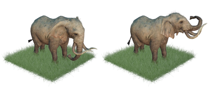
Training sequence 1    Training sequence 2

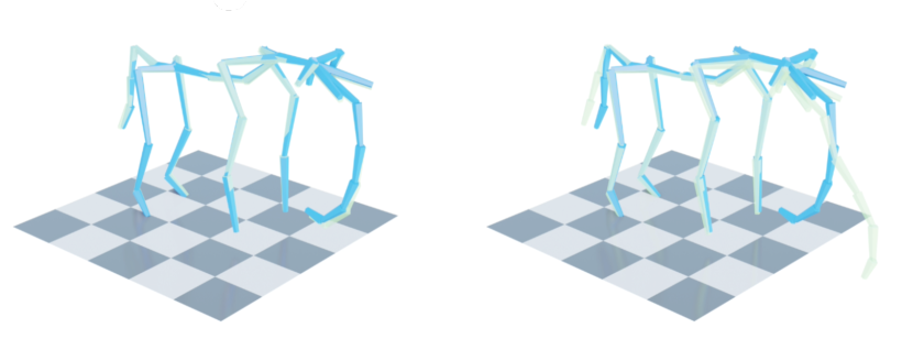
Closer to sequence 1

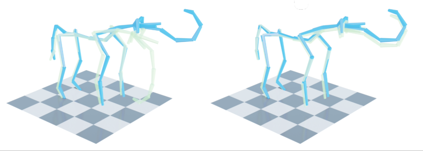
Closer to sequence 2

Figure 7. The model is trained with two sequences. The first sequence (left) contains relative static motion, the second sequence (right) contains larger movement. We visualize the skeletal animation of our generated result (blue) and its patched nearest neighbor (green) in corresponding sequences. It can be seen that our result contains the content from both training sequence.

Style transfer

Our framework can perform motion style transfer using an input animation sequence whose style is applied to the content of another input animation. We exploit the hierarchical control of the generated content at different levels of detail. Since style is often expressed in relatively high frequencies, we use the downsampling of content input ${\bf T}^{C}$ to control the generation of the neural network trained on style input ${\bf T}^{S}$ for the style transfer task. Namely, we downsample the content animation ${\bf T}^{C}$ to the corresponding coarsest resolution ${\bf T}^{C}_{1}$ and use it to replace the output of the first level of the network trained on ${\bf T}^{S}$. We demonstrate our result in Fig. 8 and the video. It can be seen that, with a single example, we successfully transfer the proud style, yielding a proud walk sharing the same pace as the content input. Due to the fact that the output is generated by multi-scale patches learned from the style input ${\bf T}^{S}$, the content of ${\bf T}^{C}$ is required to be similar to the content of ${\bf T}^{S}$, in order to generate high-quality results (e.g., both of the inputs are walking).

\begin{overpic}[width=433.62pt]{figures/style_transfer_trim.pdf} \put(-2.0,-4.0){{\color[rgb]{0.0,0.0,0.0}Style (proud)}} \put(30.0,-4.0){{\color[rgb]{0.0,0.0,0.0}Content}} \put(51.0,-4.0){{\color[rgb]{0.0,0.0,0.0}Aberman~{}\cite[citeyearpar]{(\@@bibref{Year}{aberman2020unpaired}{}{})}}} \put(88.0,-4.0){{\color[rgb]{0.0,0.0,0.0}Ours}} \end{overpic}

Figure 8. We synthesize the proud style from the style input onto the content input. It can be seen that our result contains the same content as the content input while express the proud style, e.g. higher elbow position on walking. We also show the result from  (Aberman et al., 2020b) for comparison.

Key-frame editing

Our framework can also be applied to key-frame editing (Fig. 9). We train our network on the input animation ${\bf T}$. The user can then manually edit some frames by changing their poses at the coarsest level ${\bf T}_{1}$, and the network produces smooth, realistic, and highly-detailed transitions between the modified key-frames, including unseen but plausible content.

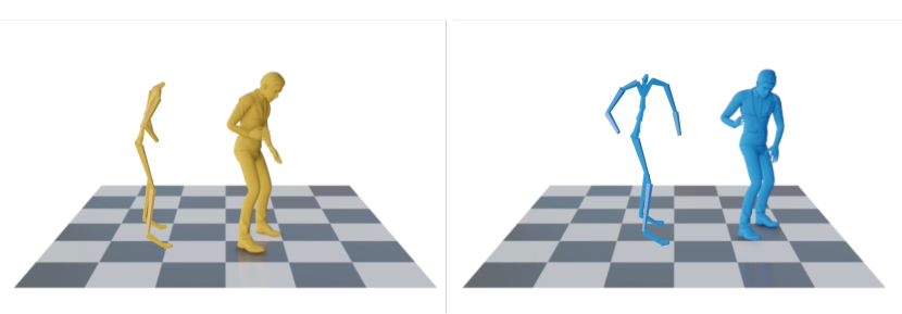
Edited Key-frames

Figure 9. We manually edit three key-frames (blue) in the input sequence by changing the poses. We visualize the result of one editing, where the character is made to face the audience. It can be seen that our model follows the editing and generates a plausible result. Please refer to the accompanying video for a complete result.

Conditional generation.

Our framework can generate motion while accounting for user-specified constraints on the motion of selected joints. Formally, given the constrained joints $\mathcal{C}$, the user-specified constraints ${\bf C}$ are given by ${\bf Q}^{\mathcal{C}}=\{{\bf Q}^{j},\ {j\in\mathcal{C}}$, where ${\bf Q}^{j}$ denotes the motion of joint $j$. In the case of motion generation with trajectory control, we set $\mathcal{C}=\{\text{root position, root orientation}\}$.

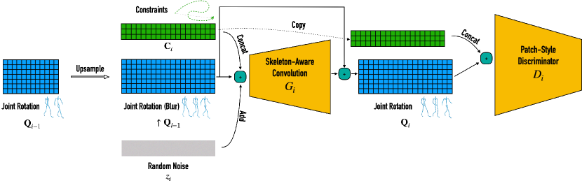
Figure 10. Training of conditional generation. To construct the input for the conditional generator, we concatenate the constraints (e.g., root joint movement) sampled from a pre-trained generator to the upsampled result generated with the same condition from the previous level. We again concatenate the constraints to the result produced by the generator and feed it to the discriminator. The discriminator ensures the correlation between constraints and the generated result.

The key component of enabling conditional generation is enforcing correlation between the generated motion and the constraints. The training process of the conditional generation is described in Fig. 10. As constraints are defined as part of the motion, we use the concatenation trick, denoted by $concat({\bf Q},{\bf C})$, during the training and inference time, where $concat({\bf Q},{\bf C})$ is the result of replacing the motion of constrained joints ${\bf Q}^{\mathcal{C}}$ in motion ${\bf Q}$ by the constraints ${\bf C}$.

For the evaluation of the $i$-th level, given the constraints at corresponding frame rate ${\bf C}_{i}$, we use $concat(\uparrow{\bf Q}_{i-1},{\bf C}_{i})$ as the input of the generator instead of the upsampled result $\uparrow{\bf Q}_{i-1}$ from the previous level. For training, we randomly generate ${\bf C}_{i}$ by sampling from a pre-trained generator mentioned above, taking the corresponding part of the motion and downsampling it to the corresponding frame rate. We employ the concatenation trick again on the output of the generator and let ${\bf Q}_{i}=concat(G_{i}(concat(\uparrow{\bf Q}_{i-1},{\bf C}_{i}),z_{i}),{\bf C}_{i})$ as the output of this stage and feed it into the discriminator. The discriminator rules out motions that do not belong to the plausible motion distribution and forces the network to generate motions complying with the given constraints.

Interactive generation.

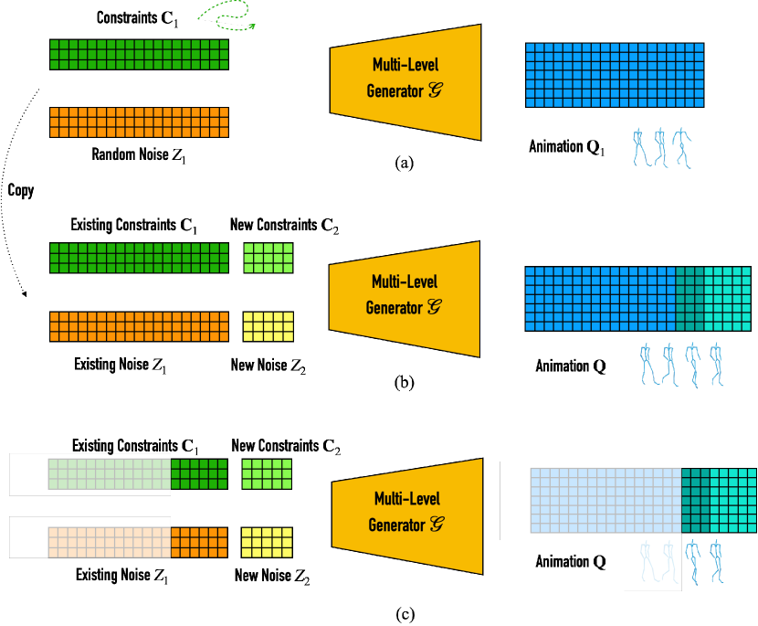
Figure 11. Interactive Generation. (a) Our conditional generation framework can be conceptually simplified as a multi-layer convolutional generator that takes user-specified constraints e.g., root joint movement, and random noise as input to generate an animation. (b) When new constraints are given, we concatenate them with the existing constraints and noise as the input for the generator. In the generated result, the frames that are outside of the receptive field of new constraints remain the same (blue area). The frames within the receptive field of new constraints are changed and are used to create a smooth transition between existing and new constraints (dark cyan). The frames complying with new constraints are generated (cyan). (c) During a generation, we only need to keep the frames within the receptive field of the dark cyan area, denoted by activated colors.

Conditional generation is particularly interesting for interactive applications, such as video games, where the motion of a character needs to be generated online in accordance to joystick controller inputs, for example. We demonstrate the process for exploiting a pre-trained conditional generation framework for such interactive application in Fig. 11. Unlike RNNs that are straightforward to use for interactive or real-time generation, convolutional neural networks generally require modifications, such as causal convolution (Oord et al., 2016). We take a different approach by exploiting the limited receptive field of convolution.

Let $\mathcal{G}({\bf C},Z)$ be the multi-level conditional generation result with constraints ${\bf C}$, where $Z$ is the set of random noise $\{z_{i}\}_{i=1}^{S}$ used during generation. In the interactive setting, we assume there are existing constraints ${\bf C}_{1}$ and the corresponding random noise $Z_{1}$, which generates the result ${\bf Q}_{1}=\mathcal{G}({\bf C}_{1},Z_{1})$, as demonstrated in Fig. 11(a). Given the new constraints ${\bf C}_{2}$ and corresponding noise $Z_{2}$, we concatenate them with ${\bf C}_{1}$ and $Z_{1}$ along the temporal axis, denoted by ${\bf C}=ext({\bf C}_{1},{\bf C}_{2})$ and $Z=ext(Z_{1},Z_{2})$, and generate a new result ${\bf Q}=\mathcal{G}({\bf C},Z)$. Denote the temporal receptive field of $\mathcal{G}(\cdot)$ by $R$ and the lengths of constraints ${\bf C}_{1}$ and ${\bf C}_{2}$ by $L_{1}$ and $L_{2}$, respectively. Note that ${{\bf Q}}^{1\,:\,L_{1}-r}$ and ${\bf Q}_{1}^{1\,:\,L_{1}-r}$ are equal (blue area in Fig. 11(b)), where ${\bf Q}^{i\,:\,j}$ denotes frame $i$ to $j$ of motion ${\bf Q}$ and $r=\lceil R/2\rceil$ is the halved receptive field. The sequence ${{\bf Q}}^{L_{1}-r+1\,:\,L_{1}}$ is different from ${\bf Q}_{1}^{L_{1}-r+1\,:\,L_{1}}$ and creates a smooth transition to the new constraints (dark cyan area in Fig. 11(b)). The remaining part ${{\bf Q}}^{L_{1}+1\,:\,L_{1}+L_{2}}$ is the newly generated result complying with the new constraints ${\bf C}_{2}$ (cyan area in Fig. 11(b)).

Therefore, given the new constraints, we only need to run the convolutional network on the concatenation of the last $2r$ frames of the existing constraints and the new constraints, as demonstrated by the activated area in Fig. 11(c), and withhold the last $r$ frames from displaying on the screen. The full method for interactive generation is summarized in Algorithm 1. We demonstrate interactive trajectory control in Fig. 12 and in the accompanying video.

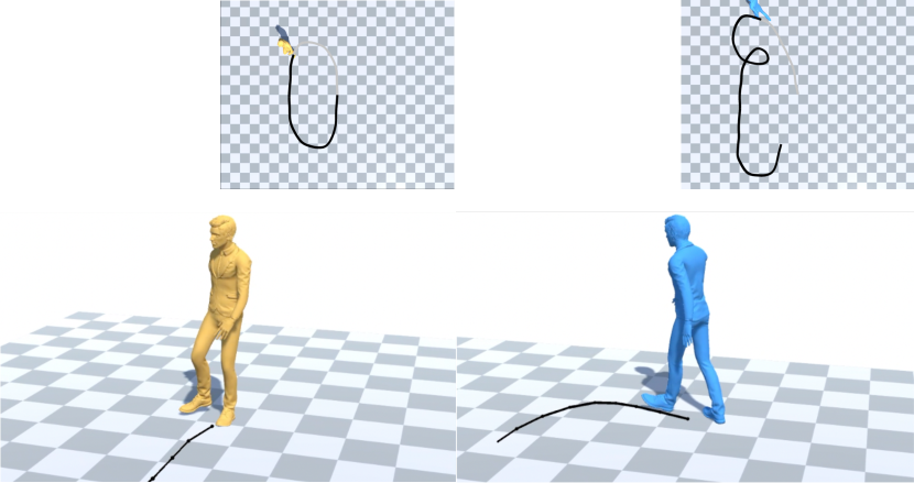
\begin{overpic}[width=433.62pt]{figures/crab_traj.pdf} \put(16.0,-5.0){{\color[rgb]{0.0,0.0,0.0}\small Input motion}} \put(62.0,-5.0){{\color[rgb]{0.0,0.0,0.0}\small Interactive generation}} \end{overpic}

Figure 12. We demonstrate the interactive trajectory control on humanoid and a hexapod crab. It can be seen that our model can cope with diverse input trajectories despite the single training sequence.

Algorithm 1 Interactive Generation

${\bf C}_{1}\leftarrow$ initial constraints

$Z_{1}\leftarrow$ inital generated noise

$r\leftarrow$ halved receptive field of $\mathcal{G}(\cdot)$

${\bf Q}\leftarrow\mathcal{G}({\bf C}_{1},Z_{1})$

Display ${\bf Q}^{1\,:\,\text{end}-r}$

while ${\bf C}_{2}\leftarrow$ new constraints do

     $Z_{2}\leftarrow$ generated noise

     ${\bf C}\leftarrow ext({\bf C}_{1},{\bf C}_{2})$

     $Z\leftarrow ext(Z_{1},Z_{2})$

     ${\bf Q}\leftarrow\mathcal{G}({\bf C},Z)$

     Display ${\bf Q}^{r+1\,:\,\text{end}-r}$

     ${\bf C}_{1}\leftarrow{\bf C}^{\text{end}-2r+1\,:\,\text{end}}$

     $Z_{1}\leftarrow Z^{\text{end}-2r+1\,:\,\text{end}}$

end while

6. Discussion and Conclusion

In this work we presented a neural motion synthesis approach that leverages the power of neural networks to exploit the information available within a single motion sequence. We demonstrated the utility of our framework on a variety of applications, including synthesizing longer motion sequences of the same essence but with plausible variations, controlled motion synthesis, key-frame editing and interpolation, and style transfer. Despite the fact that motion data is irregular, we presented a neural representation and system for effectively learning to synthesize motion. Key to our technique is a combination of skeleton-aware convolutional operators, which serve as a backbone for a progressive motion synthesis framework.

While our current framework enables interactive control of the synthesized motion trajectory, the motion essence itself has to be learned offline, in advance. In addition, our current system’s physical plausibility is limited to simple skeletal kinematics and foot contact handling. It would be interesting to incorporate higher level physics to enable synthesis of interactions and motions in complex environments. An interesting future direction is to explore online motion learning through sparse demonstrations, for example using continual learning. It is conceivable that our method could be used for data augmentation to benefit training of elaborate frameworks that require large datasets. It is also possible to explore applications of our ideas in non-skeletal settings, such as facial and other non-skeletal rigs. Our current approach does not involve the interplay of motion and shape deformation, although the latter is also an essential part of realistic character animation (e.g., geometric ground contact for creatures like snake demonstrated in the supplementary video), and we are keen on exploring this intersection in future research.

Appendix A Network Architectures

In this section, we describe the details for the network architectures.

Table 4 describes the architecture for our generator and discriminator network for a single level, where Conv and LReLU denote skeleton-aware convolution (Aberman et al., 2020a) and leaky ReLU activation respectively. All the convolution layers use reflected padding, kernel size $5$ and neighbor distance $2$. For simplicity, we denote the number of input animation features $JQ+3+|\mathcal{F}|$ by $F_{0}$.

In our experiments, we use $\lambda_{\text{adv}}=1,\lambda_{\text{rec}}=50,\lambda_{\text{con}}=5$ and $\lambda_{\text{gp}}=1$.

Name	Layers	in/out channels
Generator	Conv + LReLU	$F_{0}/F_{0}$
	Conv + LReLU	$F_{0}/2F_{0}$
	Conv + LReLU	$2F_{0}/2F_{0}$
	Conv	$2F_{0}/F_{0}$
Discriminator	Conv + LReLU	$F_{0}/F_{0}$
	Conv + LReLU	$F_{0}/2F_{0}$
	Conv + LReLU	$2F_{0}/2F_{0}$
	Conv	$2F_{0}/1$

Table 4. Network Architectures

Appendix B Solving Patched Nearest Neighbor

In this section, we describe how to solve the patched nearest neighbor (PNN). Given the generated animation ${\bf Q}$ of length $L_{Q}$ and the training animation ${\bf T}$ of length $L_{T}$, we search for the corresponding segmentation $\{l_{i}\}_{i=1}^{L_{Q}}$ for each frame in ${\bf Q}$, such that the minimum distance of any two points in the discontinuous point set $\{i\mid l_{i}\not=l_{i-1}+1\}$ is no less than $T_{\min}$.

Let $D(i)$ denotes the PNN for first $i$ frames, with boundary condition $D(0)=0$. We can solve other $D(i)$ by

(15) $$D(i) = \min_{0\leq j\leq i-T_{\min},1\leq k\leq L_{T}-i+j}D(j)+\text{cost}(j,i,k)$$

(16) $$J(i),K(i) = \operatorname*{arg\,min}_{0\leq j\leq i-T_{\min},1\leq k\leq L_{T}-i+j}D(j)+\text{cost}(j,i,k)$$

(17) $$\text{cost}(j,i,k) = \sum_{m=1}^{i-j}\|{\bf Q}^{j+m}-{\bf T}^{k+m}\|_{2}^{2},$$

where $\text{cost}(j,i,k)$ denotes the distance between ${\bf Q}^{j+1:i}$ and ${\bf T}^{k+1:k+i-j}$. After solving $D(i),J(i),K(i)$, the label $\{l_{i}\}$ can be backtraced by Algorithm 2.

Algorithm 2 Backtracing Label

$p\leftarrow L_{Q}$

while $p>0$ do

     $l_{J(p)+1:p}\leftarrow K(p)+1,K(p)+2,\cdots,K(p)+p-J(p)$

     $p\leftarrow J(p)$

end while

The $\text{cost}(j,i,k)$ can be precomputed with time complexity $O(L_{Q}^{2}L_{T})$. The dynamic programming for solving $D(i)$ also runs with time complexity $O(L_{Q}^{2}L_{T})$. The PNN cost $\mathcal{L}_{\text{PNN}}$ is given by $D(L_{Q})/L_{Q}$.