Low-Level Bi-Abduction

Abstract

The paper proposes a new static analysis designed to handle open programs, i.e., fragments of programs, with dynamic pointer-linked data structures—in particular, various kinds of lists—that employ advanced low-level pointer operations. The goal is to allow such programs be analysed without a need of writing analysis harnesses that would first initialise the structures being handled. The approach builds on a special flavour of separation logic and the approach of bi-abduction. The code of interest is analyzed along the call tree, starting from its leaves, with each function analysed just once without any call context, leading to a set of contracts summarizing the behaviour of the analysed functions. In order to handle the considered programs, methods of abduction existing in the literature are significantly modified and extended in the paper. The proposed approach has been implemented in a tool prototype and successfully evaluated on not large but complex programs.

1 Introduction

Programs with complex dynamic data structures and pointer operations are notoriously difficult to write and understand. This holds twice when a need to achieve the best possible performance drives programmers, especially those working in the C language on which we concentrate, to start using advanced low-level pointer operations such as pointer arithmetic, bit-masking information on pointers, address alignment, block operations with blocks that are split to differently sized fields (of size not known in advance), which can then be merged again, and reinterpreted differently, and so on. It may then easily happen that the resulting programs contain nasty errors, such as null-pointer dereferences, out-of-bound references, double free operations, or memory leaks, which can manifest only under some rare circumstances, may escape traditional testing, and be difficult to discover once the program is in production.

To help discover such problems (or show their absence), suitable static analyses with formal roots may help. However, the problem of analysing programs with dynamic pointer-linked data structures, sometimes referred to as shape analysis, belongs among the most difficult analysis problems, which is related to a need of efficiently encoding and handling potentially infinite sets of graph structures of in-advance unknown shape and unbounded size, corresponding to the possible memory configurations.

Moreover, the problem becomes even harder when one needs to analyse not entire programs, equipped with some analysis harness generating instances of the data structures to be handled, but just fragments of code, which simply start handling some dynamic data structures through pointers without the structures being initialised first. At the same time, in practice, the possibility of analysing code fragments is highly preferred since programmers do not like writing specialised analysis harnesses for initialising data structures of the code to be analysed (not speaking about that writing such harnesses is error-prone too). Moreover, the possibility of analysing code fragments can also help scalability of the analysis since it can then be performed in a modular way.

In this paper, we propose a new analysis designed to analyse programs and even fragments of programs with dynamic pointer-linked data structures that can use advanced low-level pointer-manipulating operations of the form mentioned above. In particular, we concentrate on sequential C programs without recursion and without function pointers manipulating various forms of lists—singly-linked, doubly-linked, circular, nested, and/or intrusive, which are perhaps the most common kind of dynamic linked data structures in practice.

Our approach uses a special flavor of separation logic (SL) [32, 23] with inductive list predicates [2] to characterize sets of program configurations. To be able to handle code fragments, we adopt the principle of bi-abductive analysis proposed over SL for analysing programs without low-level pointer operations in [6, 7]. Our work can thus be viewed as an extension of the approach of [6, 7] to programs with truly low-level operations (i.e., pointer arithmetic, bit-masking on pointers, block operations with blocks of variable size, their splitting to fields of in-advance-not-fixed size, merging such fields back, and reinterpreting them differently, etc.). As will become clear, handling such programs requires rather non-trivial changes to the abduction procedure used in [6, 7]—intuitively, one needs new analysis rules for block splitting and merging, new support for operations such as pointer plus, pointer minus, or block operations (like $\operatorname{\mathtt{memcpy}}$), and also modified support for operations like memory allocation or deallocation (to avoid deallocation of parts of blocks). Moreover, to support splitting of memory blocks to parts, gradually learning their bounds and fields, and to allow for embedding data structures into other data structures not known in advance (as commonly done, e.g., in the so-called intrusive lists), we even switch from using the traditional per-object separating conjunction in our SL to a per-field separating conjunction (as used, e.g., in [14] in the context of analysing so-called overlaid data structures), requiring separation not on the level of allocated memory blocks but their fields. As an additional benefit, our usage of per-field separating conjunction then allows us to represent more compactly even some operations on traditional data structures (without low-level pointer manipulation).

As common in bi-abductive analyses, we analyse programs, or their fragments, along their call tree, starting from the leaves of the call tree (for the time being, we assume working with non-recursive programs only). Each function is analysed just once, without any knowledge about its possible call contexts. For each function, the analysis derives a set of so-called contracts, which can then be used when this function is called from some other function higher up in the call hierarchy. A contract for a function $f$ is a pair $({\rm Phys.\leavevmode\nobreak\ Rev.\leavevmode\nobreak\ E},Q)$ where ${\rm Phys.\leavevmode\nobreak\ Rev.\leavevmode\nobreak\ E}$ is a precondition under which $f$ can be safely executed (without a risk of running into some memory error such as a null-dereference), and $Q$ is a postcondition that is guaranteed to be satisfied upon exit from $f$ provided it was called under the given precondition. Both $P$ and $Q$ are described using our flavor of SL. In fact, as also done in [6, 7], our analysis runs in two phases: the first phase derives the preconditions, while the second phase computes the postconditions. Like in [6, 7], the computed set of contracts may under-approximate the set of all possible safe preconditions of $f$ (e.g., some extreme but still safe preconditions need not be discovered). However, for each computed contract $({\rm Phys.\leavevmode\nobreak\ Rev.\leavevmode\nobreak\ E},Q)$, the post-condition $Q$ is guaranteed to over-approximate all configurations that result from calling the function under the pre-condition ${\rm Phys.\leavevmode\nobreak\ Rev.\leavevmode\nobreak\ E}$.

We have implemented our approach in a prototype tool called Broom. We have applied the tool to a selection of code fragments dealing with various kinds of lists, including very advanced implementations taken from the Linux kernel as well as the intrusive list library (for a reference, see our experimental section). Although the code is not large in the number of lines of code, it contains very advanced pointer operations, and, to the best of our knowledge, Broom is currently the only analyser that is capable of analysing many of the involved functions.

Related work

In the past (at least) 25 years there have appeared numerous approaches to automated shape analysis or, more generally, analysis of programs with unbounded dynamically-linked data structures. These approaches differ in the formalisms used for encoding sets of configurations of programs with such data structures, in their level of automation, classes of supported data structures, and/or properties of programs that are targeted by the analysis: see, e.g., [24, 33, 2, 36, 9, 38, 37, 20, 10, 3, 16, 21, 30].

Not many of the existing approaches offer a reasonably general support of low-level pointer operations (such as pointer arithmetic, address alignment, masking information on pointers, block operations, etc.). Some support of low-level pointer operations appears in multiple of these approaches, but it is often not much documented. In fact, such a support often appears in some ad hoc extension of the tool implementing the given approach only, without any description whatsoever. According to the best of our knowledge, the approach of [16], based on so-called symbolic memory graphs (SMGs), currently provides probably the most systematic and generic solution for the case of programs with low-level pointer operations and various kinds of linked lists (including advanced list implementations such as those used in the Linux kernel). Specialised approaches to certain classes of low-level programs, namely, memory allocators, then appear, e.g., in [5, 19].

In this work, we get inspired by some of the analysis capabilities of [16], but we aim at removing one of its main limitations—namely, the fact that it cannot be applied to a fragment of code. Indeed, [16] expects the analysed program to be closed, i.e., the analysed functions must be complemented by a harness that initializes all the involved data structures, which severely limits applicability of the approach in practice (since programmers are often reluctant to write specialised analysis harnesses).

Approaches allowing one to analyse open code, i.e., code fragments, with dynamic linked data structures are not frequent in the literature. Perhaps the best known of these works is the approach of bi-abduction based on separation logic with (possibly nested) list predicates proposed in [6, 7] and currently available in the Infer analyser [4]. This approach is another of the approaches that inspired our work, and we will be referring to various technical details of that paper later on. However, despite Infer contains some support of pointer arithmetic, it is not very complete (as our experiments will show), and the approach presented in [6, 7] does not at all study low-level pointer operations of the form that we aim at in this paper. Moreover, it turns out that adding a support of such operations (e.g., dealing with blocks of memory of possibly variable size, splitting them to fields of variable size, merging such fields back and reinterpreting their contents differently, having pointers with variable offsets, supporting rich pointer arithmetic, etc.) requires rather non-trivial changes and extensions to the bi-abduction mechanisms used in [6, 7].

An approach of second-order bi-abduction based also on separation logic was proposed in [27] and several follow-up papers such as [11]. The authors consider recursive programs with pointers and propose a calculus for automatic derivation of sets of equations describing the behaviour of particular functions. A solution of such a set of equations leads to a set of contracts for the considered functions. The technique is in some sense quite general—unlike [6, 7] and unlike our approach, it can even automatically learn recursive predicates describing the involved data structures, including trees, skip lists, etc. Moreover, the derivation of the equations is a cheap procedure, and no widening is needed, again unlike in [6, 7] and unlike in our approach. On the other hand, finding a solution of the generated equations is a hard problem, and the authors provide a simple heuristic designed for a specific shape of the equations only, which fails in various other cases.

Finally, we mention the Gillian project, a language-independent framework based on separation logic for the development of compositional symbolic analysis tools, including tools for whole-program symbolic execution, verification of annotated code, as well as bi-abduction [35, 34, 29, 28]. The works on Gillian concentrate on the generic framework it develops, and the published description of the supported bi-abductive analysis, perhaps most discussed in [34], is unfortunately not very detailed. In particular, it is not clear whether and how much the approach supports the low-level features of pointer manipulation that we are aiming at here (e.g., pointer arithmetic, bit-masking on addresses, etc.). According to the source code that we were able to find in the Gillian repository, the examples mentioned in the part of [34] devoted to bi-abduction do not use low-level pointer manipulation features such as pointer arithmetic. It is also mentioned in [34] that Gillian supports bi-abduction up to a predefined bound only, whereas we do not require such a bound. Further, in contrast to the present work, [34] assumes that the size of memory chunks being dynamically allocated is known, and the complex reasoning needed to resolve this issue is left for the future.

We also note that there is a vast body of work on automated decision procedures for various fragments of separation logic and problems such as satisfiability and entailment—see, e.g., [18, 22, 25, 26, 17]. However, it is not immediate how to apply these logics inside a program analysis tool. For example, the results on the cited separation logics cannot be directly applied to the (bi-)abduction problem, which is the central operation needed for a compositional program analysis. This is because the best (i.e., logically weakest) solution to the abduction problem $\varphi*[?]\models\psi$, which is a central problem for compositional program analyses, with $*$ being the separating conjunction, is given by the formula $\varphi{-\!\!\ast}\psi$, which makes use of the magic wand operator ${-\!\!\ast}$, and the cited logics do not provide support for the magic wand. This is for principle reasons: it has been observed in the literature that magic wand operators are “difficult to eliminate” [1]; further, it has been shown that adding only the singly-linked list-segment predicate to a propositional separation logic that includes the magic wand already leads to undecidability of the satisfiability problem [13]. A notable exception is the recent work [31] on a new semantics for separation logic, which enables decidability of a propositional separation logic that includes the magic wand and the singly-linked list-segment predicate (and also discusses applications to the abduction problem); however, the fragment considered in [31] is not expressive enough to cover the low-level features considered in this work such as, pointer arithmetic, memory blocks, etc., and, at present, it is unclear whether the decidability result can be extended to a richer logic. For the above reasons, we will in this paper not target a complete procedure for the (bi-)abduction problem, but rather, following [6, 7], develop approximate procedures and evaluate their usefulness in our case studies.

Main contributions of the paper

The paper proposes a new approach for automated bi-abductive analysis of programs and fragments of programs with pointers, different kinds of linked lists, and low-level memory operations. The approach is formalised, implemented in a prototype tool, and experimentally evaluated. In summary, we make the following contributions:

• A specialised dialect of separation logic suitable for automated abductive analysis of programs with lists and low-level memory operations (we use a separating conjunction between single fields and not whole memory blocks as in related approaches, and support fields of unknown and even variable size as well as unknown block boundaries).

• Contracts for basic programming statements that reflect our low-level memory model (see, e.g., the contracts of the malloc and free statements), and support for specific statements that permit low-level pointer manipulation (e.g., pointer addition).

• A set of rules for automated abductive analysis, which not only includes variants of rules from related approaches, but also new kinds of rules required for handling low-level memory operations (e.g., block splitting).

• A prototype implementation that supports bit-precise reasoning based on a reduction of (un-)satisfiability of separation logic to (un-)satisfiability of SMT over the bit-vectors.

• An experimental evaluation of the approach on a number of challenging programs.

2 An Illustration of the Approach on an Example

Before we start with a systematic description of our approach, we present its core ideas on an example. We will consider the code manipulating cyclic doubly-linked lists shown in Fig. 1. The example is inspired by the principle of intrusive lists (as used, e.g., in Linux kernel lists) where all list operations are defined on some simple list-linking structure that is then nested into user-defined structures. It is these user-defined structures that carry the data actually stored in the lists. The list manipulating functions, however, know nothing about these larger structures. However, the fact that contracts (summaries) derived for functions dealing with the small linking structures are later to be applied on the larger, user-defined structures is already problematic for some existing analyses. When providing an introduction to the approach, we will try to informally explain the involved notions, yet, due to the complexity of the issues, some prior knowledge of separation logic with inductive list predicates, e.g., [2], and ideally also bi-abduction analysis [6, 7] is helpful.

struct dll { struct dll *next, *prev; };
struct emb_dll {int value; struct dll link; };

void init_dll(struct dll *x) {

1. 1. ${\rm Phys.\leavevmode\nobreak\ Rev.\leavevmode\nobreak\ E}\equiv x=X,\quad Q\equiv x=X$

2. x–>next = x;

   1. ${\rm Phys.\leavevmode\nobreak\ Rev.\leavevmode\nobreak\ E}\equiv X\mapsto L_{1}*x=X,\quad Q\equiv X\mapsto X*x=X$

3. x–>prev = x;

   1. ${\rm Phys.\leavevmode\nobreak\ Rev.\leavevmode\nobreak\ E}\equiv X\mapsto L_{1}*X+8\mapsto L_{2}*\mathfrak{b}(X)=\mathfrak{b}(X+8)*x=X,\\ Q\equiv X\mapsto X*X+8\mapsto X*\mathfrak{b}(X)=\mathfrak{b}(X+8)*x=X$

} summary:

1. ${\rm Phys.\leavevmode\nobreak\ Rev.\leavevmode\nobreak\ E}\equiv X\mapsto L_{1}*X+8\mapsto L_{2}*\mathfrak{b}(X)=\mathfrak{b}(X+8)*x=X,\\ Q\equiv X\mapsto X*X+8\mapsto X*\mathfrak{b}(X)=\mathfrak{b}(X+8)*x=X$

void insert_after(struct dll *l, *j) {

1. 1. ${\rm Phys.\leavevmode\nobreak\ Rev.\leavevmode\nobreak\ E}\equiv l=L*j=J,\quad Q\equiv l=L*j=J$

2. struct dll *n = l–>next;

   1. ${\rm Phys.\leavevmode\nobreak\ Rev.\leavevmode\nobreak\ E}\equiv L\mapsto N*l=L*j=J,\quad Q\equiv L\mapsto N*l=L*j=J*n=N$

3. j–>next = n;

   1. ${\rm Phys.\leavevmode\nobreak\ Rev.\leavevmode\nobreak\ E}\equiv L\mapsto N*J\mapsto B_{1}*l=L*j=J,\quad Q\equiv L\mapsto N*J\mapsto N*l=L*j=J*n=N$

4. j–>prev = l;

   1. ${\rm Phys.\leavevmode\nobreak\ Rev.\leavevmode\nobreak\ E}\equiv L\mapsto N*J\mapsto B_{1}*J+8\mapsto B_{2}*\mathfrak{b}(J)=\mathfrak{b}(J+8)*l=L*j=J,\\ Q\equiv L\mapsto N*J\mapsto N*J+8\mapsto L*\mathfrak{b}(J)=\mathfrak{b}(J+8)*l=L*j=J*n=N$

5. l–>next = j;

   1. ${\rm Phys.\leavevmode\nobreak\ Rev.\leavevmode\nobreak\ E}\equiv L\mapsto N*J\mapsto B_{1}*J+8\mapsto B_{2}*\mathfrak{b}(J)=\mathfrak{b}(J+8)*l=L*j=J,\\ Q\equiv L\mapsto J*J\mapsto N*J+8\mapsto L*\mathfrak{b}(J)=\mathfrak{b}(J+8)*l=L*j=J*n=N$

6. n–>prev = j;

   1. ${\rm Phys.\leavevmode\nobreak\ Rev.\leavevmode\nobreak\ E}\equiv L\mapsto N*J\mapsto B_{1}*J+8\mapsto B_{2}*N+8\mapsto B_{3}*\mathfrak{b}(J)=\mathfrak{b}(J+8)*\mathfrak{b}(N)=\mathfrak{b}(N+8)*l=L*j=J,\\ Q\equiv L\mapsto J*J\mapsto N*J+8\mapsto L*N+8\mapsto J*\mathfrak{b}(J)=\mathfrak{b}(J+8)*\mathfrak{b}(N)=\mathfrak{b}(N+8)*l=L*\\ j=J*n=N$

} summary:

1. ${\rm Phys.\leavevmode\nobreak\ Rev.\leavevmode\nobreak\ E}\equiv L\mapsto N*J\mapsto B_{1}*J+8\mapsto B_{2}*N+8\mapsto B_{3}*\mathfrak{b}(J)=\mathfrak{b}(J+8)*\mathfrak{b}(N)=\mathfrak{b}(N+8)*l=L*j=J,\\ Q\equiv L\mapsto J*J\mapsto N*J+8\mapsto L*N+8\mapsto J*\mathfrak{b}(J)=\mathfrak{b}(J+8)*\mathfrak{b}(N)=\mathfrak{b}(N+8)*l=L*j=J$

int main() {

1. 1. ${\rm Phys.\leavevmode\nobreak\ Rev.\leavevmode\nobreak\ E}\equiv\mathsf{emp},\quad Q\equiv\mathsf{emp}$

2. struct emb_dll *x = malloc(sizeof(struct emb_dll));

   1. ${\rm Phys.\leavevmode\nobreak\ Rev.\leavevmode\nobreak\ E}\equiv\mathsf{emp},\quad Q\equiv\exists X.\ X\mapsto\top[24]*X=\mathfrak{b}(X)*x=X$

3. init_dll(&(x–>link));

   1. ${\rm Phys.\leavevmode\nobreak\ Rev.\leavevmode\nobreak\ E}\equiv\mathsf{emp},\quad Q\equiv\exists X,L_{1}.\ X\mapsto\top[8]*L_{1}\mapsto L_{1}*L_{1}+8\mapsto L_{1}*X=\mathfrak{b}(X)=\mathfrak{b}(L_{1})=\mathfrak{b}(L_{1}+8)*\\ L_{1}=X+8*x=X$

4. struct emb_dll *i = malloc(sizeof(struct emb_dll));

   1. ${\rm Phys.\leavevmode\nobreak\ Rev.\leavevmode\nobreak\ E}\equiv\mathsf{emp},\quad Q\equiv\exists I,X,L_{1}.\ I\mapsto\top[24]*X\mapsto\top[8]*L_{1}\mapsto L_{1}*L_{1}+8\mapsto L_{1}*L_{1}=X+8*X=\mathfrak{b}(X)=\mathfrak{b}(L_{1})=\mathfrak{b}(L_{1}+8)*I=\mathfrak{b}(I)*x=X*i=I$

5. init_dll(&(i–>link));

   1. ${\rm Phys.\leavevmode\nobreak\ Rev.\leavevmode\nobreak\ E}\equiv\mathsf{emp},\quad Q\equiv\exists I,X,L_{1},L_{2}.\ i\mapsto\top[8]*L_{2}\mapsto L_{2}*L_{2}+8\mapsto L_{2}*X\rightarrow\top[8]*L_{1}\mapsto L_{1}*L_{1}+8\mapsto L_{1}*L_{2}=I+8*L_{1}=X+8*X=\mathfrak{b}(X)=\mathfrak{b}(L_{1})=\mathfrak{b}(L_{1}+8)*I=b(I)=b(L_{2})=b(L_{2}+8)*x=X*i=I$

6. insert_after(&(x–>link), &(i–>link));

   1. ${\rm Phys.\leavevmode\nobreak\ Rev.\leavevmode\nobreak\ E}\equiv\mathsf{emp},\quad Q\equiv\exists I,X,L_{1},L_{2}.\ I\mapsto\top[8]*L_{2}\mapsto L_{1}*L_{2}+8\mapsto L_{1}*X\mapsto\top[8]*L_{1}\mapsto L_{2}*L_{1}+8\mapsto L_{2}*L_{2}=I+8*L_{1}=X+8*X=\mathfrak{b}(X)=b(L_{1})=\mathfrak{b}(L_{1}+8)*I=\mathfrak{b}(I)=\mathfrak{b}(L_{2})=\mathfrak{b}(L_{2}+8)*\\ x=X*i=I$

7. …

}

Figure 1: An illustrative example of a code working with cyclic doubly-linked lists and its analysis. The C expressions like ptr->field can be seen as syntactic sugar for expressions using pointer arithmetic of the form *(ptr + offsetof(field)). The $\mathfrak{e}(X)$ predicates representing the end of the block pointed by X are dropped from the $({\rm Phys.\leavevmode\nobreak\ Rev.\leavevmode\nobreak\ E},Q)$ pairs for simplicity.

In the code of our illustrative example, the function init_dll creates an initial cyclic doubly-linked list consisting of a single node. The function insert_after can then insert a new element into the list after its item pointed by $l$.

Let us note that while the code of the example in Fig. 1 may seem to not use pointer arithmetic, the code in fact uses pointer arithmetic on the level of the intermediate code we analyse. Indeed, each expression x–>field is translated to *(x+offsetof(field)). It is of course true that once all the types and fields are known and fixed, one can avoid dealing with pointer arithmetic in this case. On the other hand, the fact that we systematically handle it through pointer arithmetic allows us to smoothly handle even the cases when the types and offsets stop being known and/or constant (upon which approaches based on dealing with field names fail).

As indicated already in the introduction, we analyse the given code fragment according to its call tree, starting from the leaves (assuming there is no recursion). Each function is analysed just once, without any call context. If successful, the analysis derives a set of contracts for the given function where each contract is a pair $({\rm Phys.\leavevmode\nobreak\ Rev.\leavevmode\nobreak\ E},Q)$ consisting of a (conjunctive) pre-condition and (a possibly disjunctive) post-condition. In our introductory example, we will restrict ourselves to the simplest case, namely, having a single, purely conjunctive contract. In the contracts, both the pre- and post-condition are expressed as SL formulae. The analysis is compositional in that contracts derived for some functions are then used when analysing functions higher up in the call hierarchy (moreover, we will view even particular pointer manipulating statements as special atomic functions and describe them by pre-defined contracts).

As indicated already in the introduction, we analyse the given code fragment according to its call tree, starting from the leaves (assuming there is no recursion). Each function is analysed just once, without any call context. If successful, the analysis derives a set of contracts for the given function where each contract is a pair $({\rm Phys.\leavevmode\nobreak\ Rev.\leavevmode\nobreak\ E},Q)$ consisting of a (conjunctive) pre-condition and (a possibly disjunctive) post-condition. In our introductory example, we will restrict ourselves to the simplest case, namely, having a single, purely conjunctive contract. In the contracts, both the pre- and post-condition are expressed as SL formulae. The analysis is compositional in that contracts derived for some functions are then used when analysing functions higher up in the call hierarchy (moreover, we will view even particular pointer manipulating statements as special atomic functions and describe them by pre-defined contracts).

We begin the illustration of our analysis by analysing the init_dll function. We start the analysis by annotating the first line by the pair $(x=X,x=X)$. In this pair, the first component is the so-far derived pre-condition of the function, and the second component is the current symbolic state of the function under analysis. Here, the variable $X$ records the value of the program variable $x$ at the beginning of the function. While $x$ will be changing in the function, $X$ will never change, and we will be able to gradually generate constraints on its value to express what must hold for $x$ at the entry of the function.

After symbolically executing the statement x->next = x, we derive that the address $X$ must correspond to some allocated memory, containing some unknown value $L_{1}$. This gives us the pre-condition $X\mapsto L_{1}$ that is an SL formula stating exactly the fact that $X$ is allocated and stores the value $L_{1}$. The symbolic state is then advanced to say that $X$ is allocated and stores the value $X$, i.e., it points to itself, which is encoded as $X\mapsto X$ in SL.

After the subsequent statement x->prev = x, assuming that we work with 64 bit (i.e., 8 bytes) wide addresses, we add to the precondition the fact that the memory address $X+8$ is allocated as well. Moreover, the formula $\mathfrak{b}(X)=\mathfrak{b}(X+8)$ says that $X$ and $X+8$ belong to the same memory block, i.e., they were, e.g., allocated using one malloc statement (in fact, we use $\mathfrak{b}(X)$ to denote the—so-far unknown—base address of the block). The symbolic state is updated by the fact that the value at the address $X+8$ is also equal to $X$, i.e., $X+8\mapsto X$.

Since there are no further statements in the function, there is no branching, no loops, and all the statements are deterministic, the final contract for the function is unique and consists of the final pre-condition ${\rm Phys.\leavevmode\nobreak\ Rev.\leavevmode\nobreak\ E}\equiv X\mapsto L_{1}*X+8\mapsto L_{2}*\mathfrak{b}(X)=\mathfrak{b}(X+8)*x=X$ and the post-condition $Q\equiv X\mapsto X*X+8\mapsto X*\mathfrak{b}(X)=\mathfrak{b}(X+8)*x=X$ obtained from the final symbolic state. Here, we use “$*$” to denote a per-field separating conjunction, which, intuitively, means that while the addresses $X$ and $X+8$, which are allocated by the formulae $X\mapsto L_{1}$ and $X+8\mapsto L_{2}$, may—though need not—belong to a single memory block, the values stored at these addresses within the block do not overlap.

The same principles are then used for the computation of the contracts for the insert_after and main functions. Here, let us just highlight a situation that happens, e.g., upon the j->next = n statement of insert_after. Notice that, in its case, the so-far computed precondition $P$ must be extended by the new requirement $J\mapsto B_{1}$, stating that $J$ must be allocated, and $Q$ is then extended by the fact $J\mapsto N$, which is the effect of executing the given statement. At the same time, however, the rest of the previously computed symbolic state of the program $Q$ stays untouched (in general, only some part may be preserved). Given the current symbolic state $Q$ and a statement, the problem of deriving which precondition is missing and which part of the state will remain untouched is denoted as the bi-abduction problem, and a procedure looking for its solution is a bi-abduction procedure. The computed missing part of the pre-condition is called the anti-frame, and the computed part of the current symbolic state not modified by the statement being executed is called the frame.

When analysing the main function, one does already need not re-analyse the init_dll and insert_after functions—instead, one simply uses their contracts. For simplicity, we assume here that malloc always succeeds, and hence even main is deterministic. After the execution of malloc, we use the special predicate $x\mapsto\top[24]$ to express that a sequence of 24 bytes of undefined contents was allocated. We allow such blocks (as well as all other kinds of blocks that arise during the analysis) be split to smaller parts whenever this is needed for applying a contract of some function (or statement). That happens, e.g., on lines $b$ and $d$ of the main function where the block $X\mapsto\top[24]$ created by malloc is split to 3 fields as described by $X\mapsto\top[8]*X+8\mapsto\top[8]*X+16\mapsto\top[8]$. The last two of the fields then match the precondition of init_dll, and the first one becomes a frame (untouched by the function).

Without now going into further details, we note that analysing more complex functions requires one to solve multiple more problems. For example, if there appears some non-determinism, one needs to start working with contracts with disjunctive post-conditions and even with sets of such contracts. If the code contains loops, one needs to prevent the analysis from diverging while generating more and more points-to predicates. For that, one can use widening in the form of a list abstraction. The resulting over-approximation may then, however, render some generated pre-/post-condition pairs unsound, leading to a need to run another phase of the analysis that will start from the computed pre-conditions and check, without using abduction any more, what post-condition the code can really guarantee. We will discuss all these issues in detail in the following.

However, before proceeding, let us stress how significantly the above-mentioned use of the per-field separation distinguishes our approach from its predecessor bi-abduction analysis [6, 7]. That analysis would use whole-block predicates of the form $X\mapsto dll(next:A,prev:B)$ to describe instances of struct dll, while we use the formula $X\mapsto A*X+8\mapsto B*\mathfrak{b}(X)=\mathfrak{b}(X+8)$. The per-field separating conjunction allows us to (1) express partial information about a block and (2) infer a precondition where two (or more) fields can be in the same block as well as in different blocks. Point 1 helps us to generate contracts of functions where we do not know the exact sizes of the allocated block—e.g., init_dll does not require the pointer $x$ to point to an instance of struct dll, it can be, e.g., used on larger structures, such as, e.g., struct emb_dll, that embed the original structure. Point 2 is used in the contract of insert_after where the formula $L\mapsto N*N+8\mapsto B_{3}$ describes a memory where it may be that $L=N$ as well as $L\neq N$. The contract for insert_after can then be applied on a circular doubly-linked list consisting of a single item ($L=N$) as well on lists consisting of more items ($L\neq N$)—see Fig. 2 for an illustration.

Figure 2: An illustration of the two possible input configurations of the insert_after procedure

Note that when one uses the whole-block predicate, the precondition of insert_after in the form $L\mapsto dll(next:N,prev:\_)*N\mapsto dll(next:\_,prev:B_{3})*J\mapsto dll(next:B_{1},prev:B_{2})$ requires $L\neq N$, and hence it is not covering the two above mentioned cases. One can of course sacrifice performance of the analysis and generate multiple contracts by modifying the abduction rules—e.g., one can non-deterministically introduce an alias $L=N$ before inferring the anti-frame on line $v$ of main to get the pre-condition $L\mapsto dll(next:L,prev:\_)*L=N$. Introducing such non-determinism is, however, costly. That is why, as we will see in our experiments, it is not done in tools such as Infer, which can then cause that such tools will miss some function contracts (or generate incomplete contracts that will not be applicable in some common cases: such as insertion into a list of length 1).

An additional Example is provided in Appendix B, where pointer arithmetic and bit-masking are directly visible in the C-code.

3 Memory Model

In the following, we introduce the memory model that we use in this paper. Values are sequences of bytes, i.e., $\mathit{Val}=\mathit{Byte}^{+}$, where bytes are 8-bit words. Sequences of bytes can be interpreted as numbers—either signed or unsigned, which we leave as a part of the operations to be applied on the sequences (including conversion operations). We designate a subset of the values $\mathit{Loc}=\mathit{Byte}^{N}\subseteq\mathit{Val}$ as locations where $N\geq 1$ is the byte-width of words of a given architecture and where byte sequences to be interpreted as locations are always understood as unsigned. The $\mathsf{null}$ pointer is represented by $0\in\mathit{Loc}$ in our memory model.

We will use so-called stack-block-memory triplets (SBM triplets for short) as configurations of our memory model in order to define the operational semantics of programs (and also to define the semantics of our separation logic later on):

Stack. We assume some set of variables $\mathit{Var}$ where each variable $x\in\mathit{Var}$ has some fixed positive size, denoted as $\mathsf{size}(x)$. Then, $\mathit{Stack}$ is the set of total functions $\mathit{Var}\rightarrow\mathit{Val}$ such that each variable is mapped to a byte sequence whose length is according to the size of the variable, i.e., for each stack $S\in\mathit{Stack}$ and variable $x\in\mathit{Var}$, we have $S(x)\in\mathit{Byte}^{\mathsf{size}(x)}$.

Memory. $\mathit{Mem}$ is the set of partial functions $\mathit{Loc}\rightharpoonup\mathit{Byte}$ that define the contents of allocated memory locations.

Blocks. We use $\mathit{Interval}=\{\leavevmode\nobreak\ [l,u)\leavevmode\nobreak\ \mid\leavevmode\nobreak\ l<u\leavevmode\nobreak\ \text{where}\leavevmode\nobreak\ l,u\in\mathit{Loc}\}$ to denote intervals of subsequent memory locations where we include the lower bound and exclude the upper bound. Intuitively, an interval $[l,u)\in\mathit{Interval}$ will denote which locations were allocated at the same time (and must thus also be deallocated together, can be subtracted using pointer subtraction, etc.). $\mathit{Block}=\{\leavevmode\nobreak\ [l,u)\in\mathit{Interval}\mid l\neq 0\}$ are intervals whose lower bound is not 0 (recall that $\mathsf{null}$ is represented by $0\in\mathit{Loc}$ in our memory model). $\mathit{Blocks}\subseteq(\mathbf{2}_{\mathit{fin}})^{\mathit{Block}}$ is the set of all finite sets of non-overlapping blocks, i.e., for all $B\in\mathit{Blocks}$ and for all $[l_{1},u_{1}),[l_{2},u_{2})\in B$ such that either $l_{1}\neq l_{2}$ or $u_{1}\neq u_{2}$, we have that either $u_{1}\leq l_{2}$ or $u_{2}\leq l_{1}$.

Configurations. $\mathit{Config}$ consists of all triplets $(S,B,M)\in\mathit{Stack}\times\mathit{Blocks}\times\mathit{Mem}$ such that the set of allocated blocks and the locations whose contents is defined are linked as follows:

• For every $\ell\in\mathit{Loc}$ s.t. $M(\ell)$ is defined, there is a block $[l,u)\in B$ s.t. $\ell\in[l,u)$.

We introduce functions $\mathfrak{b}_{B},\mathfrak{e}_{B}:\mathit{Loc}\rightarrow\mathit{Loc}$, parameterized by some set of blocks $B\in\mathit{Blocks}$, which return the base or end address, respectively, of the block to which a given location belongs, i.e., given some $\ell\in\mathit{Loc}$, we set $\mathfrak{b}_{B}(\ell)=l$ in case there is some $[l,u)\in B$ with $\ell\in[l,u)$, and $\mathfrak{b}_{B}(\ell)=0$, otherwise. Likewise for $\mathfrak{e}_{B}(\ell)$.

Axioms. For later use, we note that, building on the above notation, we can express the requirements for locations to be within their associated block and for blocks to be non-overlapping in the form of the following two axioms:

$$\forall\ell.\ \mathfrak{b}_{B}(\ell)=0\vee\mathfrak{b}_{B}(\ell)\leq\ell<\mathfrak{e}_{B}(\ell)$$

$$\forall\ell,\ell^{\prime}.\ (0<\mathfrak{b}_{B}(\ell)<\mathfrak{e}_{B}(\ell^{\prime})\leq\mathfrak{e}_{B}(\ell)\vee 0<\mathfrak{b}_{B}(\ell^{\prime})<\mathfrak{e}_{B}(\ell)\leq\mathfrak{e}_{B}(\ell^{\prime}))\rightarrow\\ \mathfrak{b}_{B}(\ell)=\mathfrak{b}_{B}(\ell^{\prime})\wedge\mathfrak{e}_{B}(\ell)=\mathfrak{e}_{B}(\ell^{\prime})$$

Notation. Given a (partial) function $f$, $f[a\hookrightarrow b]$ denotes the (partial) function identical to $f$ up to $f[a\hookrightarrow b](a)=b$. Moreover, $f[a\hookrightarrow\bot]$ denotes the (partial) function identical to $f$ up to being undefined for $a$.

4 A Low-level Language and Its Operational Semantics

We now state a simple low-level language together with its operational semantics. The language is close to common intermediate languages into which programs in C are compiled by compilers such as gcc or clang. We assume that a type checker ensures that variables of the right sizes are used, guaranteeing, in particular, that the left-hand side (LHS) and right-hand side (RHS) of an assignment are of the same size or that the dereference operator is only applied to locations. We do not include the operators of item access (. and ->) nor indexing ([]) into our language as their usage can be compiled to using pointers, pointer arithmetic, and the dereference operator (*) as indeed commonly done by compilers. Likewise, we do not include the address-of operator (&) whose usage can be replaced by storing all objects whose address should be derived via & into dynamically allocated memory, followed by using pointers to such memory, as also done automatically by some compilers. Further, we assume the sizeof and offsetof operators be resolved and transformed to constants.

We now present the statements of our low-level language together with their operational semantics. The semantics is defined over configurations, which we introduced in the previous section. The semantics maintains the following invariant:

• For every $[l,u)\in B$ and every $\ell\in[l,u)$, $M(\ell)$ is defined.

We start with rules describing various assignment statements possibly combined with pointer dereferences either on the LHS or RHS. In the rules (and further on), we use $M[\ell,\ell^{\prime})$ to denote the byte sequence $M(\ell)M(\ell+1)\cdots M(\ell^{\prime}-1)$:

$$(S,B,M)\xrightarrow{x:=k}(S[x\hookrightarrow k],B,M)\text{ for some value }k\in\mathit{Val}$$

$$(S,B,M)\xrightarrow{x:=y}(S[x\hookrightarrow S(y)],B,M)$$

$$(S,B,M)\xrightarrow{x:=*y}\text{ if }\mathfrak{b}_{B}(S(y))=0\text{ or }S(y)+\mathsf{size}(x)>\mathfrak{e}_{B}(S(y)),\\ \text{ then }\mathit{error}\text{ else }(S[x\hookrightarrow M[S(y),S(y)+\mathsf{size}(x))],B,M)$$

Note that, in the case of $x:=*y$, one needs to read $\mathsf{size}(x)$ bytes from the adress $S(y)$. This is impossible if the condition $S(y)+\mathsf{size}(x)>\mathfrak{e}_{B}(S(y))$ holds.

$$(S,B,M)\xrightarrow{*x:=y}\text{ if }\mathfrak{b}_{B}(S(x))=0\text{ or }S(x)+\mathsf{size}(y)>\mathfrak{e}_{B}(S(x)),\\ \text{ then }\mathit{error}\text{ else }(S,B,M[[S(x),S(x)+\mathsf{size}(y))\hookrightarrow S(y)])$$

We continue by memory allocation. We treat 0-sized allocations as an error. For non-zero-sized allocations, the allocation can always fail and return $\mathsf{null}$, otherwise the successfully allocated memory block is initialized with some arbitrary value:

$$(S,B,M)\xrightarrow{x=malloc(z)}\text{ if }S(z)=0\text{ then }\mathit{error}\text{ else either }(S[x\hookrightarrow\mathsf{null}],B,M)\text{ or }\\ (S[x\hookrightarrow\ell],B\cup\{[\ell,\ell+S(z))\},M[[\ell,\ell+S(z))\hookrightarrow k])\text{ for some }k\in\mathit{Byte}^{S(z)}\text{ and }\ell>0\\ \text{ such that }\ell+S(z)\leq 2^{8N}\text{ and }[\ell,\ell+S(z))\text{ does not overlap with any }[l,u)\in B$$

The $\mathsf{calloc}$ function, which nullifies the allocated block, can be defined analogically to $\operatorname{\mathtt{malloc}}$, by just changing $M[[\ell,\ell+S(z))\hookrightarrow k]$ to $M[[\ell,\ell+S(z))\hookrightarrow 0^{S(z)}]$. The $\operatorname{\mathtt{realloc}}$ function, which shrinks or enlarges a block, possibly moving it to a different memory location, can be reduced to a sequence of other statements, and so we do not introduce it explicitly for brevity.

The deallocation of memory is modelled by the following rule:

$$(S,B,M)\xrightarrow{free(x)}\text{ if }S(x)\neq\mathfrak{b}_{B}(S(x))\text{ then }\mathit{error}\\ \text{ else }(S,B\setminus\{[S(x),\mathfrak{e}_{B}(S(x)))\},M[[S(x),\mathfrak{e}_{B}(S(x)))\hookrightarrow\bot])$$

We now state rules for (unary and binary) operations excluding the operation of adding an offset to a pointer and pointer subtraction, which will be handled separately. We assume that typing will ensure the right sizes of the operands and the variables to which the results are assigned. For instance, for arithmetic operations, we expect all operands and result variables to have the same type. Unary operators can be used to model type-casting that lifts variables to the required size. Finally, note also that we do not exclude division by zero in order not to complicate the rules in aspects that are not specific for our work.

$$(S,B,M)\xrightarrow{x=y\operatorname{\mathsf{bop}}z}(S[x\hookrightarrow S(y)\operatorname{\mathsf{bop}}S(z)],B,M)$$

$$(S,B,M)\xrightarrow{x=\operatorname{\mathsf{uop}}y}(S[x\hookrightarrow\operatorname{\mathsf{uop}}S(y)],B,M)$$

The rule for adding a (possibly negative) offset to a pointer requires its pointer argument to be defined and, in accordance with the C standard, the result be within the appropriate memory block plus one byte (i.e., it may point just behind the end of the block).

$$(S,B,M)\xrightarrow{x=y\operatorname{\mathsf{ptrplus}}z}\text{ if }S(y)=0\text{ or }S(y)+S(z)<\mathfrak{b}_{B}(S(y))\text{ or }S(y)+S(z)>\mathfrak{e}_{B}(S(y)),\\ \text{ then }\mathit{error}\text{ else }(S[x\hookrightarrow S(y)+S(z)],B,M)$$

The rule for the pointer subtraction is special in that it requires its pointer operands to be defined, to have the same base, and to point inside an allocated block or just behind its end (note the usage of the interval closed at both ends in the rule).

$$(S,B,M)\xrightarrow{x=y\operatorname{\mathsf{ptrsub}}z}\text{ if }S(y)=0\text{ or }S(z)\not\in[\mathfrak{b}_{B}(S(y)),\mathfrak{e}_{B}(S(y))],\\ \text{ then }\mathit{error}\text{ else }(S[x\hookrightarrow S(y)-S(z)],B,M)$$

Further, we state the semantics of the $\operatorname{\mathtt{memcpy}}$ statement that copies $z$ bytes from an address $y$ to an address $x$ and that assumes dealing with non-overlapping source/target blocks. The effect of the $\operatorname{\mathtt{memmove}}$ statement, which can handle even overlapping blocks, can be simulated by copying the source block to a fresh block and then back, and so we skip it for brevity. For brevity, we also skip the (easy to add) $\operatorname{\mathtt{memset}}$ statement, which sets each byte of some block to a given value.

$$(S,B,M)\xrightarrow{\operatorname{\mathtt{memcpy}}(x,y,z)}\text{ if }\mathfrak{b}_{B}(S(x))=0\text{ or }\mathfrak{b}_{B}(S(y))=0\\ \text{ or }S(x)+S(z)>\mathfrak{e}_{B}(S(x))\text{ or }S(y)+S(z)>\mathfrak{e}_{B}(S(y)),\\ \text{ or }S(x)+S(z)>S(y)\text{ or }S(y)+S(z)>S(x),\\ \text{ then }\mathit{error}\text{ else }(S,B,M[[S(x),S(x)+S(z))\hookrightarrow M[S(y),S(y)+S(z))])$$

To encode conditional branching arising from conditional statements or loops, we introduce the assume statement that models conditions $x\bowtie y$ for $\bowtie\leavevmode\nobreak\ \in\{=,\neq,\leq,<,\geq,>\}$. The assume statement has a side condition which ensures that this statement can only be taken for configurations satisfying the condition:

$$(S,B,M)\xrightarrow{\operatorname{\mathtt{assume}}(x\bowtie y)}(S,B,M)\text{ under the condition that }S(x)\bowtie S(y)$$

We also introduce the assert statement that is similar to the assume statement, but it checks at runtime whether the specified condition holds, and it fails if this is not the case:

$$(S,B,M)\xrightarrow{\operatorname{\mathtt{assert}}(x\bowtie y)}\text{ if }S(x)\bowtie S(y)\text{ then }(S,B,M)\text{ else }\mathit{error}$$

We structure our programs into functions. We assume a control flow graph $(V,E,\mathit{entry},\mathit{exit})$ for each function $f(x_{1},\dots,x_{n})$, where $V$ is a set of nodes, there are dedicated nodes $\mathit{entry},\mathit{exit}\in V$, and $E\subseteq V\times V$ is a set of edges where each edge is labelled by a basic statement or a function call. We model branching and looping as usual, i.e., by having multiple outgoing control flow edges labelled by an $\operatorname{\mathtt{assume}}$ statement with appropriate conditions. For simplicity, we consider functions without a return value, not referring to global variables, having parameters passed by reference only, with the names of the parameters unique to each function, and not having local variables. We consider non-recursive functions only. Finally, when a function is called, no variable can be used as an argument twice.

In particular, let $f(x_{1},\ldots,x_{n})$, $n>0$, be a function whose body $\mathcal{B}_{f}$ uses the variables $x_{1},\ldots,x_{n}$ only. Let $f(a_{1},\ldots,a_{n})$ be a call of $f$ where the arguments $a_{i}$ are pairwise different variables. We will now define the semantics of this function call with regard to some configuration $(S,B,M)$. The definition will, however, be only partial due to the possible non-termination of $f(a_{1},\ldots,a_{n})$. Let $S_{f}$ be the stack defined by $S_{f}(x_{i})=S(a_{i})$ for all $1\leq i\leq n$. Then, we consider the execution of $\mathcal{B}_{f}$ wrt the initial configuration determined by $S_{f}$ as well as the blocks $B$ and the memory $M$ at the call of $f$: Let us assume that $(S_{f},B,M)\xrightarrow{\mathcal{B}_{f}}(S_{f}^{\prime},B^{\prime},M^{\prime})$ where $\xrightarrow{\mathcal{B}_{f}}$ denotes an execution from the $\mathit{entry}$ to the $\mathit{exit}$ of $f$ (again this definition is only partial as the execution of $\mathcal{B}_{f}$ does not need to terminate). If $\mathcal{B}_{f}$ terminates wrt configuration $(S_{f},B,M)$, we set

$$(S,B,M)\xrightarrow{f(a_{1},\ldots,a_{n})}(S^{\prime},B^{\prime},M^{\prime})$$

where $S^{\prime}$ is defined by $S^{\prime}(a_{i})=S_{f}^{\prime}(x_{i})$ for all $1\leq i\leq n$, and $S^{\prime}(y)=S(y)$ for all $y\in\mathit{Var}\setminus\{a_{1},\ldots,a_{n}\}$.

5 Separation Logic

We now introduce a separation logic that supports reasoning about low-level memory models as introduced earlier. Our separation logic (SL) has the following syntax:

$$\varphi\leavevmode\nobreak\ ::=\leavevmode\nobreak\ \varepsilon_{1}\mapsto\varepsilon_{2}\mid\varepsilon_{1}\mapsto k[\varepsilon_{2}]\mid\varepsilon_{1}\mapsto\top[\varepsilon_{2}]\mid\varphi_{1}*\varphi_{2}\mid\varphi_{1}\vee\varphi_{2}\mid\operatorname{\mathsf{ls}}_{\Lambda(x,y)}(\varepsilon_{1},\varepsilon_{2})\mid$$

$$\operatorname{\mathsf{dls}}_{\Lambda(x,y,z)}(\varepsilon_{1},\varepsilon_{2},\varepsilon_{1}^{\prime},\varepsilon_{2}^{\prime})\mid\mathsf{emp}\mid true\mid\varepsilon_{1}\bowtie\varepsilon_{2}\mid\exists x.\varphi$$

$$\bowtie\leavevmode\nobreak\ ::=\leavevmode\nobreak\ =\mid\neq\mid\leq\mid<\mid\geq\mid>\hskip 14.22636pt\varepsilon\leavevmode\nobreak\ ::=\leavevmode\nobreak\ k\mid x\mid\mathfrak{b}(\varepsilon)\mid\mathfrak{e}(\varepsilon)\mid\operatorname{\mathsf{uop}}\varepsilon\mid\varepsilon_{1}\operatorname{\mathsf{bop}}\varepsilon_{2}$$

Variables and Values. Our SL formulae are stated over the same set of variables $\mathit{Var}$ and values $\mathit{Val}$ that we introduced in the definition of our memory model. In particular, the variables $x,y,z$ and the values $k$ of our SL formulae are drawn from $\mathit{Var}$ and $\mathit{Val}$, respectively.

Size. Variables, values, operators, and expressions in our logic are typed by their size. We will only work with formulae where the variables and values respect the sizes expected by the involved operations and predicates. For every expression $\varepsilon$, we denote by $\mathsf{size}(\varepsilon)$ the size of the value to which this expression may evaluate. We remark on the choice of working with fixed sizes: We intentionally do not permit variables of variable size because (1) such variables are typically not supported by low-level languages and (2) variables of variable size allow one to model strings, which would make our language vastly more powerful (allowing one to model all kinds of string operations).

Points-To Predicates. The points-to predicate $\varepsilon_{1}\mapsto\varepsilon_{2}$ denotes that the byte sequence $\varepsilon_{2}$ is stored at the memory location $\varepsilon_{1}$. Due to we are working with expressions of fixed size, every model of $\varepsilon_{1}\mapsto\varepsilon_{2}$ must allocate exactly $\mathsf{size}(\varepsilon_{2})$ bytes. In addition, we introduce two restricted cases of points-to predicates where the RHS is of parametric size: namely, $\varepsilon_{1}\mapsto k[\varepsilon_{2}]$ and $\varepsilon_{1}\mapsto\top[\varepsilon_{2}]$ that allow us to say that $\varepsilon_{1}$ points to an array of $\varepsilon_{2}$ bytes that either all have the same constant value $k$ or have any value, respectively. These predicates allow us to, e.g., express that some block of memory is nullified, which is often crucial to know when analysing advanced implementations of dynamic data structures [16]. We lift the notion of size to the RHS of these points-to predicates as follows: $\mathsf{size}(k[y])=\mathsf{size}(\top[y])=y$. In $\varepsilon_{1}\mapsto k[\varepsilon_{2}]$, we require $k$ to be a single byte, i.e., $\mathsf{size}(k)=1$.

Notation. Given a formula $\varphi$, we write $\mathit{var}(\varphi)$ to denote the free variables of $\varphi$ (as usual a variable is free if it does appear within an existential quantification). Further, given an expression $\varepsilon$, we write $\mathit{var}(\varepsilon)$ for all variables appearing in $\varepsilon$.

Terminology. We call formulae that do not contain the disjunction operator ($\vee$) symbolic heaps. We will mostly work with symbolic heaps in this paper. Disjunctions of symbolic heaps will be only used on the RHS of (some) contracts. We call formulae that do not contain existential quantification ($\exists$) quantifier-free. Our SL contains the relational predicates $\varepsilon_{1}\bowtie\varepsilon_{2}$, which include equality and disequality; these predicates are traditionally called pure in the separation logic literature. We follow this terminology and call any separating conjunction of such predicates a pure formula.

List-Segment Predicates. List segments in our SL are parameterized by a segment predicate $\Lambda(x,y)$ or $\Lambda(x,y,z)$ for singly-linked or doubly-linked lists, respectively; see Fig. 3 for an illustration of the semantics of $\operatorname{\mathsf{ls}}_{\Lambda(x,y)}(\varepsilon_{1},\varepsilon_{2})$ and $\operatorname{\mathsf{dls}}_{\Lambda(x,y,z)}(\varepsilon_{1},\varepsilon_{2},\varepsilon_{1}^{\prime},\varepsilon_{2}^{\prime})$ for $\Lambda(x,y)\equiv x\mapsto y$ and $\operatorname{\mathsf{dls}}_{\Lambda(x,y,z)}\equiv x\mapsto z*x+8\mapsto y$. We note that our list-segment predicates only have two or three free variables, respectively, which prevents the logic from, e.g., describing non-global heap objects shared by list elements. However, more parameters could be introduced in a similar fashion to other works [2]. We have not done so here since it would complicate the notation, and we take this issue as orthogonal to the techniques we propose.

Binary and Unary Operators. $\operatorname{\mathsf{uop}}$ and $\operatorname{\mathsf{bop}}$ denote some arbitrary set of binary and unary operators, respectively. We assume this set to include at least the usual operators ($+$, $-$, $*$, $\&$, $|$, …) available in low-level languages as well as a special substring operator $\cdot[\cdot,\cdot)$ on byte sequences where $k[i,j)$ for some $k=b_{0}\cdots b_{l-1}\in\mathit{Byte}^{l}$ and $0\leq i\leq j\leq l$ denotes the byte sequence $b_{i}\cdots b_{j-1}$. Since we work with variables of fixed size, we basically assume a version of each $\operatorname{\mathsf{uop}}$ and $\operatorname{\mathsf{bop}}$ for every possible operand size. We further remark that unary operators $\operatorname{\mathsf{uop}}$ can be used for modelling the casting to different sizes.

Figure 3: An illustration of the meaning of the $\operatorname{\mathsf{ls}}_{\Lambda(x,y)}(\varepsilon_{1},\varepsilon_{2})$ and $\operatorname{\mathsf{dls}}_{\Lambda(x,y,z)}(\varepsilon_{1},\varepsilon_{2},\varepsilon_{1}^{\prime},\varepsilon_{2}^{\prime})$ formulae.

Semantics. We now define the semantics of our SL over SBM triplets $(S,B,M)\in\mathit{Config}$:

$$(S,B,M)\models\varepsilon_{1}\mapsto\varepsilon_{2}\text{ iff }\\ \operatorname{\mathsf{dom}}(M)=[\llbracket\varepsilon_{1}\rrbracket_{S,B},\llbracket\varepsilon_{1}\rrbracket_{S,B}+\mathsf{size}(\varepsilon_{2}))\text{ and }M[\llbracket\varepsilon_{1}\rrbracket_{S,B},\llbracket\varepsilon_{1}\rrbracket_{S,B}+\mathsf{size}(\varepsilon_{2}))=\llbracket\varepsilon_{2}\rrbracket_{S,B}$$

where

$$\llbracket k\rrbracket_{S,B}\leavevmode\nobreak\ =\leavevmode\nobreak\ k,\llbracket x\rrbracket_{S,B}\leavevmode\nobreak\ =\leavevmode\nobreak\ S(x),\llbracket\mathfrak{b}(\varepsilon)\rrbracket_{S,B}\leavevmode\nobreak\ =\leavevmode\nobreak\ \mathfrak{b}_{B}(\llbracket\varepsilon\rrbracket_{S,B}),\llbracket\mathfrak{e}(\varepsilon)\rrbracket_{S,B}\leavevmode\nobreak\ =\leavevmode\nobreak\ \mathfrak{e}_{B}(\llbracket\varepsilon\rrbracket_{S,B}),\\ \llbracket\operatorname{\mathsf{uop}}\varepsilon\rrbracket_{S,B}\leavevmode\nobreak\ =\leavevmode\nobreak\ \operatorname{\mathsf{uop}}(\llbracket\varepsilon\rrbracket_{S,B}),\text{ and }\llbracket\varepsilon_{1}\operatorname{\mathsf{bop}}\varepsilon_{2}\rrbracket_{S,B}\leavevmode\nobreak\ =\leavevmode\nobreak\ \llbracket\varepsilon_{1}\rrbracket_{S,B}\leavevmode\nobreak\ \operatorname{\mathsf{bop}}\leavevmode\nobreak\ \llbracket\varepsilon_{2}\rrbracket_{S,B}$$

$$(S,B,M)\models\varepsilon_{1}\mapsto k[\varepsilon_{2}]\text{ iff }\\ \operatorname{\mathsf{dom}}(M)=[\llbracket\varepsilon_{1}\rrbracket_{S,B},\llbracket\varepsilon_{1}\rrbracket_{S,B}+\llbracket\varepsilon_{2}\rrbracket_{S,B})\text{ and }M[\llbracket\varepsilon_{1}\rrbracket_{S,B}+i]=k\text{ for all }0\leq i<\llbracket\varepsilon_{2}\rrbracket_{S,B}$$

$$(S,B,M)\models\varepsilon_{1}\mapsto\top[\varepsilon_{2}]\text{ iff }\operatorname{\mathsf{dom}}(M)=[\llbracket\varepsilon_{1}\rrbracket_{S,B},\llbracket\varepsilon_{1}\rrbracket_{S,B}+\llbracket\varepsilon_{2}\rrbracket_{S,B})$$

We remark on the difference between the three points-to predicates: the predicate $\varepsilon_{1}\mapsto\varepsilon_{2}$ fixes the exact sequence of bytes $\varepsilon_{2}$ that is stored from location $\varepsilon_{1}$ onwards, and the number of bytes is known (the size of $\varepsilon_{2}$); the predicate $\varepsilon_{1}\mapsto k[\varepsilon_{2}]$ states that there are $\varepsilon_{2}$ number of bytes stored from location $\varepsilon_{1}$ onwards (note that the number of bytes $\varepsilon_{2}$ is symbolic), and each of these bytes equals $k$; and the predicate $\varepsilon_{1}\mapsto\top[\varepsilon_{2}]$ works in the same way except that the bytes stored are not fixed.

$$(S,B,M)\models\varphi_{1}*\varphi_{2}\text{ iff there are some }M_{1},M_{2}\text{ with }M=M_{1}\uplus M_{2},(S,B,M_{i})\models\varphi_{i}$$

$$(S,B,M)\models\varphi_{1}\vee\varphi_{2}\text{ iff }(S,B,M)\models\varphi_{1}\text{ or }(S,B,M)\models\varphi_{2}$$

$$(S,B,M)\models\mathsf{emp}\text{ iff }\operatorname{\mathsf{dom}}(M)=\emptyset\hskip 28.45274pt(S,B,M)\models true\text{ always holds }$$

$$(S,B,M)\models\varepsilon_{1}\bowtie\varepsilon_{2}\text{ iff }\operatorname{\mathsf{dom}}(M)=\emptyset\text{ and }\llbracket\varepsilon_{1}\rrbracket_{S,B}\bowtie\llbracket\varepsilon_{2}\rrbracket_{S,B}$$

We point out that pure formulae constrain the heap to be empty. This is typically not required by separation logics that support classical (non-separating) conjunction at least on pure sub-formulae. However, we exclude the classical conjunction in order to simplify the presentation and hence need to constrain the heap of pure formulae to be empty.

$$(S,B,M)\models\exists x.\varphi(x)\text{ iff there is some }v\in\mathit{Val}\\ \text{ and a fresh variable }u\in\mathit{Var}\text{ s.t. }(S[u\hookrightarrow v],B,M)\models\varphi(u)$$

$$(S,B,M)\models\operatorname{\mathsf{ls}}_{\Lambda(x,y)}(\varepsilon_{1},\varepsilon_{2})\text{ iff }(S,B,M)\models\varepsilon_{1}=\varepsilon_{2}\text{ or }\\ \quad\quad(S,B,M)\models\varepsilon_{1}\neq\varepsilon_{2}*\mathsf{true}\text{ and there is some }\ell\in\mathit{Loc}\\ \quad\quad\text{ and a fresh variable }u\in\mathit{Var}\text{ s.t. }(S[u\hookrightarrow\ell],B,M)\models\Lambda(\varepsilon_{1},u)*\operatorname{\mathsf{ls}}_{\Lambda(x,y)}(u,\varepsilon_{2})$$

$$(S,B,M)\models\operatorname{\mathsf{dls}}_{\Lambda(x,y,z)}(\varepsilon_{1},\varepsilon_{2},\varepsilon_{1}^{\prime},\varepsilon_{2}^{\prime})\text{ iff }(S,B,M)\models\varepsilon_{1}=\varepsilon_{2}^{\prime}*\varepsilon_{2}=\varepsilon_{1}^{\prime}\text{ or }\\ \quad\quad(S,B,M)\models\varepsilon_{1}\neq\varepsilon_{2}^{\prime}*\varepsilon_{2}\neq\varepsilon_{1}^{\prime}*\mathsf{true}\text{ and there is some }\ell\in\mathit{Loc}\text{ and a fresh variable}\\ \quad\quad u\in\mathit{Var}\text{ such that }(S[u\hookrightarrow\ell],B,M)\models\Lambda(\varepsilon_{1},u,\varepsilon_{2})*\operatorname{\mathsf{dls}}_{\Lambda(x,y,z)}(u,\varepsilon_{1},\varepsilon_{1}^{\prime},\varepsilon_{2}^{\prime})$$

Satisfiability and Entailment. We say that an SL formula $\varphi$ is satisfiable iff there is a model $(S,B,M)$ such that $(S,B,M)\models\varphi$. We say that an SL formula $\varphi_{1}$ entails an SL formula $\varphi_{2}$, denoted $\varphi_{1}\models\varphi_{2}$, iff we have that $(S,B,M)\models\varphi_{2}$ for every model $(S,B,M)$ such that $(S,B,M)\models\varphi_{1}$.

Restrictions on the Segment Predicates. From now on, we put further restrictions on the segment predicates $\Lambda(x,y)$ and $\Lambda(x,y,z)$: (1) $\Lambda$ needs to be of the shape $\exists x_{1},\ldots,x_{k}.\varphi$ for some quantifier-free symbolic heap $\varphi$. Intuitively, this condition is required since quantifier-free symbolic heaps are the formulae on which the symbolic execution described in Section 6 is based on and the existential quantification allows to hide some nested data. (2) $\Lambda$ needs to be block-closed in the sense defined below.

Block-closedness. A formula $\varphi$ is block-closed iff, for all $(S,B,M)\models\varphi$ and $\ell\in\operatorname{\mathsf{dom}}(M)$, we have that $[\mathfrak{b}(\ell),\mathfrak{e}(\ell))\subseteq\operatorname{\mathsf{dom}}(M)$. Intuitively, block-closedness ensures that all points-to assertions in a formula add up to whole blocks. We require block-closedness in order to ensure that list-segments correspond to our intuition and connect different memory blocks (i.e., we exclude models where multiple or all nodes of list-segments belong to the same block). Technically, the requirement of block-closedness makes it easier to formulate rules for materialisation of list-segment nodes in the abduction procedure and for entailment checking. We leave lifting the restriction of block-closedness for future work. A sufficient condition for block-closedness, which is easy to check, is that all points-to assertions in $\varphi$ can be organized in groups $\varepsilon_{i}\mapsto\Upsilon_{i}$, for $1\leq i\leq n$, where $\Upsilon$ represents either $y$, $k[y]$, or $\top[y]$, such that $\varepsilon_{i}=\varepsilon_{i-1}+\mathsf{size}(\Upsilon_{i})$ for all $1<i\leq n$, and $\varphi$ implies that $\mathfrak{e}(\varepsilon_{1})-\mathfrak{b}(\varepsilon_{1})=\sum_{i=1..n}\mathsf{size}(\Upsilon_{i})$.

6 Contracts of Functions and Their Generation

Our analysis is based on generating contracts of functions along the call tree, starting from its leaves. The contracts summarize the semantics of the functions under analysis. (We may also compute multiple contracts for the same function where each contract provides a valid summary of the function; the contracts might, however, differ in the preconditions under which they apply.) We introduce our notion of contracts in Subsection 6.1. We note that basic statements of our core language can be viewed as special built-in functions. Hence, we then introduce contracts for the basic statements in Subsection 6.2. These serve as the starting point of our analysis: Using the contracts of the built-in functions, we derive contracts for any function built of them as described in Subsection 6.3.

6.1 Contracts of Functions

We assume a set of variables $\mathit{Var}=\mathit{PVar}\uplus\mathit{LVar}$ that is partitioned into two disjoint infinite set of program variables $\mathit{PVar}$ and logical variables $\mathit{LVar}$ (also called ghost variables). For functions $f(x_{1},\ldots,x_{n})$ with parameters $x_{i}$, we always require $x_{1},\ldots,x_{n}\in\mathit{PVar}$ (also recall that we assume that $x_{1},\ldots,x_{n}$ are the only variables occurring in the body of $f$). To summarize the semantics of a function $f(x_{1},\ldots,x_{n})$, we use (sets of) contracts of the form $\{{\rm Phys.\leavevmode\nobreak\ Rev.\leavevmode\nobreak\ E}\}f(x_{1},\ldots,x_{n})\{Q\}$ where

• the pre-condition ${\rm Phys.\leavevmode\nobreak\ Rev.\leavevmode\nobreak\ E}$ is a quantifier-free symbolic heap, and

• the post-condition $Q$ is a disjunction of formulas of the form $\exists_{Q}.(Q_{\mathit{free}}*Q_{\mathit{eq}})$ such that $Q_{\mathit{free}}$ is a quantifier-free symbolic heap with $\mathit{var}(Q_{\mathit{free}})\subseteq\mathit{LVar}$, $Q_{\mathit{eq}}$ is the formula $x_{1}=\varepsilon_{1}*\cdots*x_{n}=\varepsilon_{n}$ for some expressions $\varepsilon_{i}$ with $\mathit{var}(\varepsilon_{i})\subseteq\mathit{LVar}$, and ${}_{Q}=(\mathit{var}(Q_{\mathit{free}}*Q_{\mathit{eq}})\cap\mathit{LVar})\setminus\mathit{var}({\rm Phys.\leavevmode\nobreak\ Rev.\leavevmode\nobreak\ E})$. Note that every disjunct of the post-condition $Q$ describes the heap by a formula over the logical variables (the formula $Q_{\mathit{free}}$) and fixes the values of the program variables in terms of expressions over the logical variables (the formula $Q_{\mathit{eq}}$) where all logical variables that do not appear in the pre-condition ${\rm Phys.\leavevmode\nobreak\ Rev.\leavevmode\nobreak\ E}$ are existentially quantified (on the other hand, those logical variables that appear in the pre-condition may be implicitly considered as universally quantified).

• We call a contract conjunctive if the post-condition $Q\equiv Q_{1}\vee\cdots\vee Q_{l}$ consists of a single disjunct (i.e., $l=1$), and disjunctive otherwise.

Soundness of contracts

We will now state what it means for a contract to be sound. As usual we stipulate that configurations satisfying the pre-condition lead to configurations satisfying the post-condition. In addition, we also require that we can always add a frame to the pre-/post-condition, i.e., a formula describing a part of the heap untouched by the function. Here, a frame $F$ is any symbolic heap with $\mathit{var}(F)\subseteq\mathit{LVar}$. A contract $\{{\rm Phys.\leavevmode\nobreak\ Rev.\leavevmode\nobreak\ E}\}f(x_{1},\ldots,x_{n})\{Q\}$ is called sound iff, for all frames $F$, all triples $(S,B,M)$ such that $(S,B,M)\models F*{\rm Phys.\leavevmode\nobreak\ Rev.\leavevmode\nobreak\ E}$, and all executions of $f(x_{1},\ldots,x_{n})$ that start from $(S,B,M)$ and end in some configuration $(S^{\prime},B^{\prime},M^{\prime})$, it holds that $(S^{\prime},B^{\prime},M^{\prime})\models F*Q$.

6.2 Contracts for Basic Statements

We give below contracts for the basic statements of our programming language stated as functions (basic statements may be viewed as special built-in functions). For simplicity (and w.l.o.g.), we assume that it never happens that the same variable appears both at the LHS and RHS of an assignment. Recall that $\mathsf{emp}$ is implicit in all otherwise pure constraints (and so we do not need to repeat it):

• Function $\operatorname{\mathtt{assign}}(x,y)$ with the body $x:=y$:

  $$\{y=Y\}\leavevmode\nobreak\ \operatorname{\mathtt{assign}}(x,y)\leavevmode\nobreak\ \{x=Y\leavevmode\nobreak\ *\leavevmode\nobreak\ y=Y\}.$$

• Function $\operatorname{\mathtt{const}}_{k}(x)$ with the body $x:=k$:

  $$\{\mathsf{emp}\}\leavevmode\nobreak\ \operatorname{\mathtt{const}}_{k}(x)\leavevmode\nobreak\ \{x=k\}.$$

• Function $\operatorname{\mathtt{load}}(x,y)$ with the body $x:=*y$:

  $$\{y=Y\leavevmode\nobreak\ *\leavevmode\nobreak\ Y\mapsto z\}\leavevmode\nobreak\ \operatorname{\mathtt{load}}(x,y)\leavevmode\nobreak\ \{x=z\leavevmode\nobreak\ *\leavevmode\nobreak\ y=Y\leavevmode\nobreak\ *\leavevmode\nobreak\ Y\mapsto z\}$$

  with $Q_{\mathit{free}}\equiv Y\mapsto z$ and $Q_{\mathit{eq}}\equiv x=z\leavevmode\nobreak\ *\leavevmode\nobreak\ y=Y$.

• Function $\operatorname{\mathtt{store}}(x,y)$ with the body $*x:=y$:

  $$\{x=X\leavevmode\nobreak\ *\leavevmode\nobreak\ y=Y\leavevmode\nobreak\ *\leavevmode\nobreak\ X\mapsto z\}\leavevmode\nobreak\ \operatorname{\mathtt{store}}(x,y)\leavevmode\nobreak\ \{x=X\leavevmode\nobreak\ *\leavevmode\nobreak\ y=Y\leavevmode\nobreak\ *\leavevmode\nobreak\ X\mapsto Y\}$$

  with $Q_{\mathit{free}}\equiv X\mapsto Y$ and $Q_{\mathit{eq}}\equiv x=X\leavevmode\nobreak\ *\leavevmode\nobreak\ y=Y$.

• Function $\operatorname{\mathtt{malloc}}(x,y)$ that either succeeds or fails to allocate memory through $x:=\operatorname{\mathtt{malloc}}(y)$:

  $$\{y=Y\}\leavevmode\nobreak\ \operatorname{\mathtt{malloc}}(x,y)\leavevmode\nobreak\ \{x=\mathsf{null}\leavevmode\nobreak\ *\leavevmode\nobreak\ y=Y\vee\exists u.\ x=u\leavevmode\nobreak\ *\leavevmode\nobreak\ \nu(u,Y)\leavevmode\nobreak\ *\leavevmode\nobreak\ y=Y\}$$

  where $\nu(u,Y)=u\mapsto\top[Y]*\mathfrak{b}(u)=u\leavevmode\nobreak\ *\leavevmode\nobreak\ \mathfrak{e}(u)=u+Y$. Note that either $Q_{\mathit{free}}\equiv\nu(u,Y)$ and $Q_{\mathit{eq}}\equiv x=u\leavevmode\nobreak\ *\leavevmode\nobreak\ y=Y$ or $Q_{\mathit{free}}\equiv\mathsf{emp}$ and $Q_{\mathit{eq}}\equiv x=\mathsf{null}\leavevmode\nobreak\ *\leavevmode\nobreak\ y=Y$. A very similar contract can be used for $\mathsf{calloc}$, just with $u\mapsto\top[Y]$ changed to $u\mapsto 0[Y]$. We remark that the contracts for $\operatorname{\mathtt{malloc}}$ and $\mathsf{calloc}$ are the only disjunctive contracts among the contracts for the basic statements of our programming language.

• Function $\operatorname{\mathtt{free}}(x)$ called with the $\mathsf{null}$ argument:

  $$\{x=X\leavevmode\nobreak\ *\leavevmode\nobreak\ X=\mathsf{null}\}\leavevmode\nobreak\ \operatorname{\mathtt{free}}(x)\leavevmode\nobreak\ \{x=X\leavevmode\nobreak\ *\leavevmode\nobreak\ X=\mathsf{null}\}$$

• Function $\operatorname{\mathtt{free}}(x)$ called over a non-$\mathsf{null}$ argument:

  $$\{x=X\leavevmode\nobreak\ *\leavevmode\nobreak\ X\mapsto\top[y]*\mathfrak{b}(X)=X\leavevmode\nobreak\ *\leavevmode\nobreak\ \mathfrak{e}(X)=X+y\}\leavevmode\nobreak\ \operatorname{\mathtt{free}}(x)\leavevmode\nobreak\ \{x=X\}$$

  Note that a block to be freed may be split into multiple fields at the time of freeing. We, however, do not need to deal with this issue here since the later presented bi-abduction rules will split the LHS of the contract of $\operatorname{\mathtt{free}}$ such that it can match the fragmented block.

• Functions $\mathtt{assign}_{\operatorname{\mathsf{bop}}}(x,y,z)$ with the body $x:=y\operatorname{\mathsf{bop}}z$ for binary operators $\operatorname{\mathsf{bop}}$ (and likewise for unary operators $\operatorname{\mathsf{uop}}$):

  $$\{y=Y\leavevmode\nobreak\ *\leavevmode\nobreak\ z=Z\}\leavevmode\nobreak\ x:=y\operatorname{\mathsf{bop}}z\leavevmode\nobreak\ \{x=Y\operatorname{\mathsf{bop}}Z\leavevmode\nobreak\ *\leavevmode\nobreak\ y=Y\leavevmode\nobreak\ *\leavevmode\nobreak\ z=Z\}$$

• Function $\operatorname{\mathsf{ptrplus}}(x,y,z)$ with the body $x:=y\operatorname{\mathsf{ptrplus}}z$ for the case when the result is within the block of the pointer to which an offset is added:

  $$\{y=Y\leavevmode\nobreak\ *\leavevmode\nobreak\ z=Z\leavevmode\nobreak\ *\leavevmode\nobreak\ \varphi_{Y,Z}\}\leavevmode\nobreak\ x:=y\operatorname{\mathsf{ptrplus}}z\leavevmode\nobreak\ \{x=Y+Z\leavevmode\nobreak\ *\leavevmode\nobreak\ y=Y\leavevmode\nobreak\ *\leavevmode\nobreak\ z=Z\leavevmode\nobreak\ *\leavevmode\nobreak\ \varphi_{Y,Z}\}$$

  for $\varphi_{Y,Z}\equiv\mathfrak{b}(Y)\neq 0\leavevmode\nobreak\ *\leavevmode\nobreak\ \mathfrak{b}(Y)=\mathfrak{b}(Y+Z)*\mathfrak{e}(Y)=\mathfrak{e}(Y+Z)$.

• Function $\operatorname{\mathsf{ptrplus}}(x,y,z)$ with the body $x:=y\operatorname{\mathsf{ptrplus}}z$ for the case when the result points one byte past the block of the pointer to which an offset is added:

  $$\{y=Y\leavevmode\nobreak\ *\leavevmode\nobreak\ z=Z\leavevmode\nobreak\ *\leavevmode\nobreak\ \varphi_{Y,Z}\}\leavevmode\nobreak\ x:=y\operatorname{\mathsf{ptrplus}}z\leavevmode\nobreak\ \{x=Y+Z\leavevmode\nobreak\ *\leavevmode\nobreak\ y=Y\leavevmode\nobreak\ *\leavevmode\nobreak\ z=Z\leavevmode\nobreak\ *\leavevmode\nobreak\ \varphi_{Y,Z}\}$$

  for $\varphi_{Y,Z}\equiv\mathfrak{b}(Y)\neq 0\leavevmode\nobreak\ *\leavevmode\nobreak\ Y+Z=\mathfrak{e}(Y)$.

• Function $\operatorname{\mathsf{ptrsub}}(x,y,z)$ with the body $x:=y\operatorname{\mathsf{ptrsub}}z$:

  $$\{y=Y\leavevmode\nobreak\ *\leavevmode\nobreak\ z=Z\leavevmode\nobreak\ *\leavevmode\nobreak\ \varphi_{Y,Z}\}\leavevmode\nobreak\ x:=y\operatorname{\mathsf{ptrsub}}z\leavevmode\nobreak\ \{x=Y-Z\leavevmode\nobreak\ *\leavevmode\nobreak\ y=Y\leavevmode\nobreak\ *\leavevmode\nobreak\ z=Z\}$$

  for $\varphi_{Y,Z}\equiv\mathfrak{b}(Y)\neq 0\leavevmode\nobreak\ *\leavevmode\nobreak\ \mathfrak{b}(Y)\leq Z\leq\mathfrak{e}(Y)$.

• To deal with the $\operatorname{\mathtt{memcpy}}(x,y,z)$ statement, we use the below contract schema encoding concrete contracts for all the ways the address spaces $[x,x+z)$ and $[y,y+z)$ can be divided into $m,n\geq 1$ fields, respectively:

  $$\{\varphi_{X,Y,Z}\leavevmode\nobreak\ *\leavevmode\nobreak\ \varphi_{X,Z}\leavevmode\nobreak\ *\leavevmode\nobreak\ \varphi_{Y,Z}\}\leavevmode\nobreak\ \operatorname{\mathtt{memcpy}}(x,y,z)\leavevmode\nobreak\ \{\varphi_{X,Y,Z}\leavevmode\nobreak\ *\leavevmode\nobreak\ \varphi^{\prime}_{X,Z}*\varphi_{Y,Z}\}$$

  where

  • $\varphi_{X,Y,Z}\equiv x=X\leavevmode\nobreak\ *\leavevmode\nobreak\ y=Y\leavevmode\nobreak\ *\leavevmode\nobreak\ z=Z$,

  • $\varphi_{X,Z}\equiv X\mapsto\top[Z]$,

  • $\varphi_{Y,Z}\equiv Y_{1}=Y*\bigstar_{i=1}^{i\leq n}(Y_{i}\mapsto B_{i}*Y_{i+1}=Y_{i}+\mathsf{size}(B_{i}))*Y_{n+1}=Y+Z$,

  • $\varphi^{\prime}_{X,Z}\equiv X_{1}=X*\bigstar_{i=1}^{i\leq n}(X_{i}\mapsto B_{i}*X_{i+1}=X_{i}+\mathsf{size}(B_{i}))*X_{n+1}=X+Z$.

  Of course, in practice, a particular instance of the contract schema will be chosen on-the-fly according to the current state of the computation. One starts with $\varphi_{Y,Z}\equiv Y\mapsto B$ and $\varphi^{\prime}_{X,Z}\equiv X\mapsto B$ and uses the splitting bi-abduction rules on $\varphi_{Y,Z}$ according to how the block pointed by $Y$ is partitioned. This splitting is synchronized with splitting $\varphi^{\prime}_{X,Z}$ in the same way. Thus, the $Z$ bytes stored at $Y$ will be transferred to $X$ preserving their interpretation.

• Function $\operatorname{\mathtt{assume}}_{\bowtie}(y,z)$ with the body $\operatorname{\mathtt{assume}}(y\bowtie z)$:

  $$\{y=Y\leavevmode\nobreak\ *\leavevmode\nobreak\ z=Z\}\leavevmode\nobreak\ \operatorname{\mathtt{assume}}(y\bowtie z)\leavevmode\nobreak\ \{y=Y\leavevmode\nobreak\ *\leavevmode\nobreak\ z=Z\leavevmode\nobreak\ *\leavevmode\nobreak\ y\bowtie z\}$$

• Function $\operatorname{\mathtt{assert}}_{\bowtie}(y,z)$ with the body $\operatorname{\mathtt{assert}}(y\bowtie z)$:

  $$\{y=Y\leavevmode\nobreak\ *\leavevmode\nobreak\ z=Z\leavevmode\nobreak\ *\leavevmode\nobreak\ y\bowtie z\}\leavevmode\nobreak\ \operatorname{\mathtt{assert}}(y\bowtie z)\leavevmode\nobreak\ \{y=Y\leavevmode\nobreak\ *\leavevmode\nobreak\ z=Z\leavevmode\nobreak\ *\leavevmode\nobreak\ y\bowtie z\}$$

We now state the soundness of the contracts for the basic statement of our programming language:

Lemma 6.1.

Let $\mathit{stmt}$ be a basic statement and let $\{{\rm Phys.\leavevmode\nobreak\ Rev.\leavevmode\nobreak\ E}\}\ f(x_{1},\ldots,x_{n})\ \{Q\}$ be a contract for $\mathit{stmt}$ as stated above. Then, the contract is sound, i.e., for all frames $F$, all configurations $(S,B,M)$ such that $(S,B,M)\models F*{\rm Phys.\leavevmode\nobreak\ Rev.\leavevmode\nobreak\ E}$, and all executions of $f(x_{1},\ldots,x_{n})$ that start from $(S,B,M)$ and end in some configuration $(S^{\prime},B^{\prime},M^{\prime})$, it holds that $(S^{\prime},B^{\prime},M^{\prime})\models F*Q$.

Proof 6.2.

Direct from the semantics of our programming language as stated in Section 4.

6.3 Contract Generation

We now discuss the generation of contracts for arbitrary user-defined functions. Our analysis proceeds along the call tree, starting from its leaves. Hence, we can assume to already have computed contracts for nested function calls. (Recall that, in this paper, we limit ourselves to non-recursive functions.) We first discuss a special case where we assume that the function to be analyzed consists of a sequence of calls of other functions (i.e., no branching and looping), and we assume the contracts of the nested function calls to be conjunctive. After that we state the general set-up of our analysis.

6.3.1 Sequences of Function Calls with Conjunctive Contracts

We now consider functions whose body consists of a sequence of function calls $s_{1};\ldots;s_{l}$ for some $l>0$, whose contracts are conjunctive (this includes for example all built-in functions apart from $\operatorname{\mathtt{malloc}}$). We formulate a symbolic execution that, given such a function $f(x_{1},\ldots,x_{n})$, derives a sound contract for $f$. The symbolic execution starts at the beginning of $f$ and maintains a pair of formulae ${\rm Phys.\leavevmode\nobreak\ Rev.\leavevmode\nobreak\ E}$ and $Q$, representing the so-far computed part of the pre-condition of the function $f$ and the current symbolic state. The symbolic execution will guarantee that configurations that satisfy ${\rm Phys.\leavevmode\nobreak\ Rev.\leavevmode\nobreak\ E}$ lead to configurations satisfying $Q$ after executing the so-far analysed statements. ${\rm Phys.\leavevmode\nobreak\ Rev.\leavevmode\nobreak\ E}$ and $Q$ will change throughout the symbolic execution because we keep restricting the precondition ${\rm Phys.\leavevmode\nobreak\ Rev.\leavevmode\nobreak\ E}$ and advancing the symbolic state $Q$. The symbolic execution is set up such that the program variables $x_{1},\ldots,x_{n}$ may be updated, while all other variables will never be modified (but, of course, fresh variables may be introduced and assigned at any time). The symbolic execution is initialised by introducing fresh logical variables $X_{1},\ldots,X_{n}$ and setting ${\rm Phys.\leavevmode\nobreak\ Rev.\leavevmode\nobreak\ E}\equiv Q\equiv x_{1}=X_{1}*\cdots*x_{n}=X_{n}$. The symbolic execution then proceeds iteratively, considering the sequences $s_{1};\ldots;s_{i}$, starting with $i=0$. For every $0\leq i\leq l$, the formulae ${\rm Phys.\leavevmode\nobreak\ Rev.\leavevmode\nobreak\ E}$ and $Q$ are updated such that they form a contract for the sequence $s_{1};\ldots;s_{i}$. We argue in the proof of Theorem 6.4 below that the symbolic execution maintains the contract $\{{\rm Phys.\leavevmode\nobreak\ Rev.\leavevmode\nobreak\ E}\}\ s_{1};\ldots;s_{i}\ \{Q\}$. Note that our initialization of the formulae ${\rm Phys.\leavevmode\nobreak\ Rev.\leavevmode\nobreak\ E}$ and $Q$ ensures the correctness condition for $i=0$ and we derive a sound contract for $f$ once we reach $i=l$.

We now describe how to apply a contract for a function call $s_{i}$. We consider some function $\{C\}g(y_{1},\ldots,y_{m})\{D\}$ with $D\equiv\exists_{D}.\ D_{\mathit{free}}*D_{\mathit{eq}}$. Let $s_{i}\equiv g(a_{1},\ldots,a_{m})$ be the function call with arguments $\{a_{1},\ldots,a_{m}\}\subseteq\{x_{1},\ldots,x_{n}\}$, where we have by assumption that the $a_{i}$ are pairwise different. Let ${\rm Phys.\leavevmode\nobreak\ Rev.\leavevmode\nobreak\ E}$ and $Q\equiv\exists_{Q}.\ Q_{\mathit{free}}*Q_{\mathit{eq}}$ be the current pre-condition and symbolic state, respectively. We can assume w.l.o.g. that $\mathit{var}(C)\cap\mathit{var}(Q_{\mathit{free}}*Q_{\mathit{eq}})\subseteq\mathit{PVar}$ because we can always rename the logical variables of a contract (here, $\{C\}\ g(y_{1},\ldots,y_{m})\ \{D\}$) in order to avoid name clashes. Then, we consider the bi-abduction problem

$$Q_{\mathit{free}}*[?]\models C^{\prime}*[?]\quad\quad\quad\quad(\mathtt{BAP})$$

where

$$C^{\prime}\equiv(C[a_{i}/y_{i}])[\varepsilon_{j}/x_{j}]$$

is the formula $C$ from the precondition of $g(y_{1},\ldots,y_{m})$ with the parameters $y_{i}$ substituted by the arguments $a_{i}$, and the variables $x_{j}$ substituted by the expressions $\varepsilon_{j}$ according to the formula $Q_{\mathit{eq}}\equiv x_{1}=\varepsilon_{1}*\cdots*x_{n}=\varepsilon_{n}$. (Note that no formula in the bi-abduction problem contains any of the program variables $x_{1},\ldots,x_{n},y_{1},\ldots,y_{m}$.) A solution to the bi-abduction problem ($\mathtt{BAP}$) consists of formulae $M$ and $F$, denoted as an antiframe and a frame, respectively, such that

$$Q_{\mathit{free}}*M\models\exists.\ C^{\prime}*F\quad\quad\text{ where }\quad\quad=\mathit{var}(C^{\prime}*F)\setminus\mathit{var}(Q_{\mathit{free}}*Q_{\mathit{eq}}*M).$$

We require $M$ to be a quantifier-free symbolic heap with $\mathit{var}(M)\subseteq\mathit{LVar}\setminus_{Q}$ (note that all existentially quantified variables in _Q are introduced during the symbolic execution, hence we cannot restrict them at the beginning of the function where they are not known yet). We also require $F$ to be a quantifier-free symbolic heap with $\mathit{var}(F)\subseteq\mathit{LVar}$. Note that any such $M$ and $F$ ensure that the function call $s_{i}\equiv g(a_{1},\ldots,a_{m})$ can be safely executed: The soundness of the contract $\{C\}\ g(y_{1},\ldots,y_{m})\ \{D\}$ guarantees that $g(y_{1},\ldots,y_{m})$ can be executed for any valuation of the universally quantified variables; hence, it is sufficient to find some valuation (as required by the existential quantification in $\exists.\ C^{\prime}*F$). Given a solution $M$ and $F$ to the bi-abduction problem ($\mathtt{BAP}$), we can then update the current state of the symbolic execution (we denote the new pre- and post-condition by ${\rm Phys.\leavevmode\nobreak\ Rev.\leavevmode\nobreak\ E}_{\mathit{after}}$ and $Q_{\mathit{after}}$, respectively):

• ${\rm Phys.\leavevmode\nobreak\ Rev.\leavevmode\nobreak\ E}_{\mathit{after}}:=M*{\rm Phys.\leavevmode\nobreak\ Rev.\leavevmode\nobreak\ E}$.

• $Q_{\mathit{free}}^{\prime}:=F*D_{\mathit{free}}$.

• $Q_{\mathit{eq}}^{\prime}$ is the (separating) conjunction of $x_{i}=\varepsilon_{j}^{\prime}$ for each $x_{i}$ passed by reference as the argument $a_{j}$ to $g$ where $a_{j}=\varepsilon_{j}^{\prime}$ is the final value according to the post-condition $D_{\mathit{eq}}$; and $x_{i}=\varepsilon_{i}$ for each variable not passed to $g$ where $x_{i}=\varepsilon_{i}$ is according to $Q_{\mathit{eq}}$ before the call of $g$.

• $Q_{\mathit{after}}:=\exists_{Q_{\mathit{after}}}.\ Q_{\mathit{free}}^{\prime}*Q_{\mathit{eq}}^{\prime}$ where ${}_{Q_{\mathit{after}}}=(\mathit{var}(Q_{\mathit{free}}^{\prime}*Q_{\mathit{eq}}^{\prime})\cap\mathit{LVar})\setminus\mathit{var}({\rm Phys.\leavevmode\nobreak\ Rev.\leavevmode\nobreak\ E}_{\mathit{after}})$.

For later use, we write $({\rm Phys.\leavevmode\nobreak\ Rev.\leavevmode\nobreak\ E}_{\mathit{after}},Q_{\mathit{after}}):=\mathit{biabduct}({\rm Phys.\leavevmode\nobreak\ Rev.\leavevmode\nobreak\ E},Q,g(a_{1},\ldots,a_{m}),C,D)$ for the result of advancing the symbolic execution by one step wrt the bi-abduction solution.

Formula Simplification by Quantifier Elimination. We will always try to simplify formulas with existentially quantified formulas. For this, we assume the existence of a quantifier elimination procedure $\mathtt{eliminate}(,\varphi)$, which attempts to eliminate as many variables $u\in$ as possible from a quantifier-free symbolic heap $\varphi$. We require that $\exists^{\prime}.\psi$ is equivalent to $\exists.\varphi$, where $\psi=\mathtt{eliminate}(,\varphi)$ is the formula returned by the quantifier elimination procedure and ^′ is the set minus the eliminated variables. We use the following simple quantifier elimination procedure $\mathtt{eliminate}(,\varphi)$ in our implementation: For every equality in $u=\varepsilon$ in $\varphi$ with $u\in$, we replace $u$ everywhere in $\varphi$ by $\varepsilon$ and then delete the equality $u=\varepsilon$. It is easy to verify that this procedure satisfies the above requirement.

Example 6.3.

We consider the call $g(x)$ of a function with contract $\left\{C\right\}g(y)\left\{D\right\}$ during the analysis of some function $f(x)$, where the so-far derived precondition ${\rm Phys.\leavevmode\nobreak\ Rev.\leavevmode\nobreak\ E}$, the current symbolic state $Q$ as well as the pre- and post-conditions $C$ and $D$ look as follows:

• ${\rm Phys.\leavevmode\nobreak\ Rev.\leavevmode\nobreak\ E}\equiv X\mapsto a*X+8\mapsto b*x=X$;

• $Q\equiv\exists_{Q}.\ Q_{\mathit{free}}*Q_{\mathit{eq}}$ where $Q_{\mathit{free}}\equiv X\mapsto a*X+8\mapsto z$, $Q_{\mathit{eq}}\equiv x=X$ and ${}_{Q}=\{z\}$;

• $C\equiv Y\mapsto u*Y+8\mapsto w*u\mapsto v*y=Y$, and

• $D\equiv\exists c.\ D_{\mathit{free}}*D_{\mathit{eq}}$ where $D_{\mathit{free}}\equiv Y\mapsto u*Y+8\mapsto w*u\mapsto v*v\mapsto c$ and $D_{\mathit{eq}}\equiv y=v$.

The formula $C^{\prime}$ wrt which we will be solving the bi-abduction problem will look as follows:

$$C^{\prime}\equiv(C[x/y])[X/x]\equiv Y\mapsto u*Y+8\mapsto w*u\mapsto v*X=Y.$$

Hence, we need to solve the bi-abduction problem

$$X\mapsto a*X+8\mapsto z*[?]\models Y\mapsto u*Y+8\mapsto w*u\mapsto v*X=Y*[?].$$

Then, our bi-abduction procedure returns

$$M\equiv a\mapsto v\quad\quad\text{and}\quad\quad F\equiv X=Y*a=u*z=w,$$

i.e., we have

$$Q_{\mathit{free}}*M\models\exists.\ C^{\prime}*F\quad\text{ where }\quad=\mathit{var}(C^{\prime}*F)\setminus\mathit{var}(Q_{\mathit{free}}*Q_{\mathit{eq}}*M)=\{Y,u,w\}.$$

(For how $M$ and $F$ were generated, see the description of the bi-abduction procedure below.) The new missing precondition ${\rm Phys.\leavevmode\nobreak\ Rev.\leavevmode\nobreak\ E}_{\mathit{after}}$ of the function $f(x)$ and the new current symbolic state $Q_{\mathit{after}}$ of $f(x)$ after the call of $g(x)$ is then as follows:

• ${\rm Phys.\leavevmode\nobreak\ Rev.\leavevmode\nobreak\ E}_{\mathit{after}}\equiv{\rm Phys.\leavevmode\nobreak\ Rev.\leavevmode\nobreak\ E}*M\equiv X\mapsto a*X+8\mapsto b*x=X*a\mapsto v$,

• $Q_{\mathit{free}}^{\prime}\equiv F*D_{\mathit{free}}\equiv X=Y*a=u*z=w*Y\mapsto u*Y+8\mapsto w*u\mapsto v*v\mapsto c$,

• $Q^{\prime}_{\mathit{eq}}\equiv x=v$,

• $Q_{\mathit{after}}\equiv\exists c,u,w,Y,z.\ X=Y*a=u*z=w*Y\mapsto u*Y+8\mapsto w*u\mapsto v*v\mapsto c*x=v$,

• we then intend to simplify $Q_{\mathit{after}}$ and compute

  $$\mathtt{eliminate}(\{c,u,w,Y,z\},Q_{\mathit{free}}^{\prime}*Q^{\prime}_{\mathit{eq}})\equiv X\mapsto a*X+8\mapsto w*a\mapsto v*v\mapsto c*x=v,$$

  i.e., we obtain

  $$Q_{\mathit{after}}^{\mathit{simp}}\equiv\exists c,w.\ X\mapsto a*X+8\mapsto w*a\mapsto v*v\mapsto c*x=v.$$

We now state the soundness of our approach:

Theorem 6.4.

Let $f(x_{1},\ldots,x_{n})$ be some function and let $\{{\rm Phys.\leavevmode\nobreak\ Rev.\leavevmode\nobreak\ E}\}\ f(x_{1},\ldots,x_{n})\ \{Q\}$ by the contract inferred by the bi-abductive inference as stated above. Then, the contract is sound, i.e., for all frames $F$, all configurations $(S,B,M)$ with $(S,B,M)\models F*{\rm Phys.\leavevmode\nobreak\ Rev.\leavevmode\nobreak\ E}$, and all executions of $f(x_{1},\ldots,x_{n})$ that start with $(S,B,M)$ and end with some configuration $(S^{\prime},B^{\prime},M^{\prime})$ we have $(S^{\prime},B^{\prime},M^{\prime})\models F*Q$.

Proof 6.5.

We prove that $\left\{{\rm Phys.\leavevmode\nobreak\ Rev.\leavevmode\nobreak\ E}\right\}s_{1};\ldots;s_{i}\left\{Q\right\}$ for all $0\leq i\leq l$ (*), where ${\rm Phys.\leavevmode\nobreak\ Rev.\leavevmode\nobreak\ E}$ and $Q$ are the formulae after step $i$ of the symbolic execution. We prove (*) by induction on $i$. Note that (*) holds for $i=0$ due to the initialization of ${\rm Phys.\leavevmode\nobreak\ Rev.\leavevmode\nobreak\ E}$ and $Q$.

We now consider some $i>0$ and the sequence $s_{1};\ldots;s_{i}$. By induction assumption we have that $\left\{{\rm Phys.\leavevmode\nobreak\ Rev.\leavevmode\nobreak\ E}\right\}s_{1};\ldots;s_{i}\left\{Q\right\}$. Let $s_{i+1}\equiv g(a_{1},\ldots,a_{m})$ be some function call for which we assume the contract $\{C\}\ g(y_{1},\ldots,y_{m})\ \{D\}$ with $D\equiv\exists_{D}.\ D_{\mathit{free}}*D_{\mathit{eq}}$, whose soundness has already been established. Let $M$ and $F$ be a solution to the biabuction problem, i.e., let $M$ and $F$ be formulae with $Q_{\mathit{free}}*M\models\exists.\ C^{\prime}*F$ for $=\mathit{var}(C^{\prime}*F)\setminus\mathit{var}(Q_{\mathit{free}}*Q_{\mathit{eq}}*M)$ (#) where $C^{\prime}$ is the formula $C$ after parameter instantiation as described above. We will now argue that $\left\{{\rm Phys.\leavevmode\nobreak\ Rev.\leavevmode\nobreak\ E}_{\mathit{after}}\right\}s_{1};\ldots;s_{i};s_{i+1}\left\{Q_{\mathit{after}}\right\}$ where ${\rm Phys.\leavevmode\nobreak\ Rev.\leavevmode\nobreak\ E}_{\mathit{after}}$ and $Q_{\mathit{after}}$ are the pre- and post-condition after step $i+1$. Let $G$ be some frame. We now instantiate the frame in the induction assumption with $G*M$, i.e., we have that $\left\{G*M*{\rm Phys.\leavevmode\nobreak\ Rev.\leavevmode\nobreak\ E}\right\}s_{1};\ldots;s_{i}\left\{G*M*Q\right\}$. Let $(S,B,M)$ be some configuration with $(S,B,M)\models G*M*{\rm Phys.\leavevmode\nobreak\ Rev.\leavevmode\nobreak\ E}$ and let $(S^{\prime},B^{\prime},M^{\prime})$ be the result of executing $s_{1};\ldots;s_{i}$ starting from configuration $(S,B,M)$. From the instantiation of the induction assumption, we get that $(S^{\prime},B^{\prime},M^{\prime})\models G*M*Q$. By (#), we have that $(S^{\prime},B^{\prime},M^{\prime})\models G*\exists_{Q}.\ (Q_{\mathit{eq}}*\exists.\ (C^{\prime}*F))$. Hence, there is some stack $S^{\prime\prime}$ with $\operatorname{\mathsf{dom}}(S^{\prime\prime})=\operatorname{\mathsf{dom}}(S^{\prime})\cup_{Q}\cup\cup\{y_{1},\ldots,y_{m}\}$ such that $(S^{\prime\prime},B^{\prime},M^{\prime})\models G*F*C$ and $S^{\prime\prime}(y_{j})=S^{\prime\prime}(x_{i})$ according to $x_{i}=a_{j}$ in the function call $g(a_{1},\ldots,a_{m})$. Let $(S^{\prime\prime\prime},B^{\prime\prime},M^{\prime\prime})$ be the configuration that results from executing $g(y_{1},\ldots,y_{m})$ starting from $(S^{\prime\prime},B^{\prime},M^{\prime})$. By the correctness of $\{C\}\ g(y_{1},\ldots,y_{m})\ \{D\}$, we get that $(S^{\prime\prime\prime},B^{\prime\prime},M^{\prime\prime})\models G*F*D$. We now consider the stack $S^{\circ}$ defined by $S^{\circ}(x_{i})=S^{\prime\prime\prime}(y_{j})$ for all $1\leq i\leq m$ with $x_{i}=a_{j}$ in the function call $g(a_{1},\ldots,a_{m})$, and $S^{\circ}(x_{i})=S(x_{i})$ for all $x_{i}\in\mathit{Var}\setminus\{a_{1},\ldots,a_{n}\}$. Note that $(S^{\circ},B^{\prime\prime},M^{\prime\prime})$ is the resulting configuration after returning from the function call $g(a_{1},\ldots,a_{m})$. By the above, we then have $(S^{\circ},B^{\prime\prime},M^{\prime\prime})\models G*\exists(\cup_{Q}\cup_{D}).\ (F*D_{\mathit{free}}*Q_{\mathit{eq}}^{\prime})$. Because of $(\cup_{Q}\cup_{D})\cap\mathit{var}({\rm Phys.\leavevmode\nobreak\ Rev.\leavevmode\nobreak\ E}_{\mathit{after}})=\emptyset$, we then get $(S^{\circ},B^{\prime\prime},M^{\prime\prime})\models G*\exists_{Q_{\mathit{after}}}.\ (Q_{\mathit{free}}^{\prime}*Q_{\mathit{eq}}^{\prime})$. This establishes the claim.

6.3.2 Branching, Looping and Disjunctive Contracts

So far we have described the generation of contracts for functions $\left\{{\rm Phys.\leavevmode\nobreak\ Rev.\leavevmode\nobreak\ E}\right\}f(x_{1},\dots,x_{n})\left\{Q\right\}$ whose body consists of a sequence of function calls with conjunctive contracts and without branching and looping. In this section, we lift all these restrictions. We follow [7] and present a two-round analysis for the general case (we present a short summary of these two analysis phases here to make the paper self-contained, but we refer the reader to [7] for a more detailed exposition and for a formal statement on the soundness of the analysis): The first round (called PreGen in [7]) infers a set of pre-/post-condition pairs $({\rm Phys.\leavevmode\nobreak\ Rev.\leavevmode\nobreak\ E},Q)$, but in contrast to Theorem 6.4 there is no guarantee about the soundness of the inferred $({\rm Phys.\leavevmode\nobreak\ Rev.\leavevmode\nobreak\ E},Q)$. For each pre-/post-condition pair $({\rm Phys.\leavevmode\nobreak\ Rev.\leavevmode\nobreak\ E},Q)$ computed in the first round, the second round (called PostGen in [7]) discards the post-condition $Q$ and re-starts the symbolic execution from the pre-condition ${\rm Phys.\leavevmode\nobreak\ Rev.\leavevmode\nobreak\ E}$ not allowing the strengthening of the pre-condition throughout the symbolic execution, which either fails or results in a set of pre-/post-condition pairs $({\rm Phys.\leavevmode\nobreak\ Rev.\leavevmode\nobreak\ E},Q_{1}),\ldots,({\rm Phys.\leavevmode\nobreak\ Rev.\leavevmode\nobreak\ E},Q_{l})$. In the latter case, we return $({\rm Phys.\leavevmode\nobreak\ Rev.\leavevmode\nobreak\ E},Q_{1}\vee\cdots\vee Q_{l})$, which is guaranteed to be a sound contract.

We now describe the general set-up that is used by the first as well as the second analysis round. Recall that we assume a control flow graph $(V,E,\mathit{entry},\mathit{exit})$ for each function $f(x_{1},\dots,x_{n})$ where $V$ is a set of nodes, there are dedicated nodes $\mathit{entry},\mathit{exit}\in V$, and $E\subseteq V\times V$ is a set of edges where each edge is labelled by a function call (recall that we also model basic statements as functions). By $V_{\mathit{cut}}\subseteq V$, we denote a set of cut-points, where each loop must contain at least one cut-point (usually the header location of a loop). A function without loops has $V_{\mathit{cut}}=\emptyset$. The symbolic execution maintains a mapping $\mathit{symb}:V\rightarrow(\mathbf{2}_{\mathit{fin}})^{\mathit{Contract}}$ where each location $v\in V$ is mapped to a finite set of pre-/post-condition pairs $({\rm Phys.\leavevmode\nobreak\ Rev.\leavevmode\nobreak\ E},Q)\in\mathit{Contract}$. Initially, $\mathit{symb}(\mathit{entry})=\left\{({\rm Phys.\leavevmode\nobreak\ Rev.\leavevmode\nobreak\ E}_{\mathit{init}},Q_{\mathit{init}})\right\}$ where ${\rm Phys.\leavevmode\nobreak\ Rev.\leavevmode\nobreak\ E}_{\mathit{init}}$ and $Q_{\mathit{init}}$ are specified as stated below for the first and second analysis round, and $\mathit{symb}(v)=\emptyset$ for all $v\neq\mathit{entry}$.

The symbolic execution then proceeds as a work-list algorithm. In each computational step, the symbolic execution picks a pre-/post-condition pair $({\rm Phys.\leavevmode\nobreak\ Rev.\leavevmode\nobreak\ E},Q)\in\mathit{symb}(v)$, for some $v\in V$, that has not been processed yet. Then, the symbolic execution performs the following for each outgoing edge $(v,v^{\prime})\in E$: Let $g(a_{1},\dots,a_{k})$ be the function call labelling the edge $(v,v^{\prime})$. For each contract $\left\{C\right\}g(y_{1},\dots,y_{k})\left\{D_{1}\vee\cdots\vee D_{l}\right\}$ and each disjunct $D_{i}$ of such a contract, we invoke bi-abduction procedure from Section 6.3, i.e., let $({\rm Phys.\leavevmode\nobreak\ Rev.\leavevmode\nobreak\ E}_{\mathit{after}},Q_{\mathit{after}})=\mathit{biabduct}({\rm Phys.\leavevmode\nobreak\ Rev.\leavevmode\nobreak\ E},Q,g(a_{1},\ldots,a_{m}),C,D_{i})$; then,

1. for $v^{\prime}\not\in V_{\mathit{cut}}$, we add $({\rm Phys.\leavevmode\nobreak\ Rev.\leavevmode\nobreak\ E}_{\mathit{after}},Q_{\mathit{after}})$ into $\mathit{symb}(v^{\prime})$, and

2. for $v^{\prime}\in V_{\mathit{cut}}$,

   • we check whether there is a $({\rm Phys.\leavevmode\nobreak\ Rev.\leavevmode\nobreak\ E}^{\prime},Q^{\prime})\in\mathit{symb}(v^{\prime})$ that covers $({\rm Phys.\leavevmode\nobreak\ Rev.\leavevmode\nobreak\ E}_{\mathit{after}},Q_{\mathit{after}})$, i.e., we have $\exists\mathit{LVar}({\rm Phys.\leavevmode\nobreak\ Rev.\leavevmode\nobreak\ E}_{\mathit{after}}).\ {\rm Phys.\leavevmode\nobreak\ Rev.\leavevmode\nobreak\ E}_{\mathit{after}}\models\exists\mathit{LVar}({\rm Phys.\leavevmode\nobreak\ Rev.\leavevmode\nobreak\ E}^{\prime}).\ {\rm Phys.\leavevmode\nobreak\ Rev.\leavevmode\nobreak\ E}^{\prime}$ and $\exists\mathit{LVar}(Q_{\mathit{after}}).\ Q_{\mathit{after}}\models\exists\mathit{LVar}(Q^{\prime}).\ Q^{\prime}$, where $\mathit{LVar}(\varphi)=\mathit{var}(\varphi)\cap\mathit{LVar}$ denotes the free logical variables appearing in the formula; we note that a covering guarantees that the all configurations that satisfy the pre- resp. post condition of the pair $({\rm Phys.\leavevmode\nobreak\ Rev.\leavevmode\nobreak\ E}_{\mathit{after}},Q_{\mathit{after}})$ already satisfy the corresponding condition of $({\rm Phys.\leavevmode\nobreak\ Rev.\leavevmode\nobreak\ E}^{\prime},Q^{\prime})$ (for some suitable instantiation of the logical variables); hence, such $({\rm Phys.\leavevmode\nobreak\ Rev.\leavevmode\nobreak\ E}_{\mathit{after}},Q_{\mathit{after}})$ do not need to be added to $\mathit{symb}(v^{\prime})$, which supports the termination of the fixed point termination;

   • if there is no $({\rm Phys.\leavevmode\nobreak\ Rev.\leavevmode\nobreak\ E}^{\prime},Q^{\prime})\in\mathit{symb}(v^{\prime})$ that covers $({\rm Phys.\leavevmode\nobreak\ Rev.\leavevmode\nobreak\ E}_{\mathit{after}},Q_{\mathit{after}})$, we add $(\alpha({\rm Phys.\leavevmode\nobreak\ Rev.\leavevmode\nobreak\ E}_{\mathit{after}}),\alpha(Q_{\mathit{after}}))$ into $\mathit{symb}(v^{\prime})$, where $\alpha$ is a widening procedure in the form of a list abstraction that is quite common in the area—cf., e.g., [2]. In its simplest form, the abstraction $\alpha$ searches for patterns of the form $\Lambda(x,y)*\Lambda(y,z)$ (resp. $\Lambda(x,v,y)*\Lambda(y,x,z)$) and replaces them by $\operatorname{\mathsf{ls}}_{\Lambda(a,b)}(x,z)$ (resp. $\operatorname{\mathsf{dls}}_{\Lambda(a,b,c)}(x,y,v,z)$) provided that there is no pointer nor other list segment incoming to $y$ (i.e., the current symbolic state cannot, e.g., imply $u\mapsto y*u\neq x$). The actual abstraction is, of course, more complex—e.g., apart from applying to sequences of the $\Lambda$ predicates as above, which of course can be longer than just two appearances of $\Lambda$, it also applies to sequences consisting of the $\Lambda$ predicates and of compatible singly-/doubly-linked list segments (e.g., $\Lambda(x,y)*\operatorname{\mathsf{ls}}_{\Lambda(a,b)}(y,z)$ may abstract to $\operatorname{\mathsf{ls}}_{\Lambda(a,b)}(x,z)$). Since, however, the abstraction is rather standard in the area, we do not develop it further here and refer the interested reader to [2].

The worklist algorithm continues until a fixed point is reached, i.e., until no more pre-/post-condition pairs are added to $\mathit{symb}$ and all pairs have been processed.

Next, we add some more specific details about the two rounds of the analysis:

1. Round:

We set ${\rm Phys.\leavevmode\nobreak\ Rev.\leavevmode\nobreak\ E}_{\mathit{init}}\equiv Q_{\mathit{init}}\equiv x_{1}=X_{1}*\cdots*x_{n}=X_{n}$ (recall that we assume $x_{1},\dots,x_{n}$ to be all the program variables that appear in the body of $f(x_{1},\dots,x_{n})$). Once the worklist algorithm has reached a fixed point, we return all pre-/post-condition pairs $({\rm Phys.\leavevmode\nobreak\ Rev.\leavevmode\nobreak\ E},Q)\in\mathit{symb}(\mathit{exit})$ as the result of the first analysis round.

2. Round:

For each $({\rm Phys.\leavevmode\nobreak\ Rev.\leavevmode\nobreak\ E},Q)$ computed by the first analysis round, there is a second analysis round where we set ${\rm Phys.\leavevmode\nobreak\ Rev.\leavevmode\nobreak\ E}_{\mathit{init}}\equiv Q_{\mathit{init}}\equiv{\rm Phys.\leavevmode\nobreak\ Rev.\leavevmode\nobreak\ E}$ and where we disallow the strengthening of the pre-condition throughout the symbolic execution (i.e., we require $M=\mathsf{emp}$ for each bi-abduction call performed during symbolic execution; if this is not the case, we fail). Once the worklist algorithm has reached a fixed point, we consider the computed pre-/post-condition pairs $\mathit{symb}(\mathit{exit})=\{({\rm Phys.\leavevmode\nobreak\ Rev.\leavevmode\nobreak\ E},Q_{1}),\ldots,({\rm Phys.\leavevmode\nobreak\ Rev.\leavevmode\nobreak\ E},Q_{l})\}$ (note that all these pairs must have the same pre-condition ${\rm Phys.\leavevmode\nobreak\ Rev.\leavevmode\nobreak\ E}$) and return the contract $({\rm Phys.\leavevmode\nobreak\ Rev.\leavevmode\nobreak\ E},Q_{1}\vee\cdots\vee Q_{l})$. We point out to the reader that the second round in general creates multiple contracts—one contract for each possible pre-condition.

Assume and Assert Statements

As we have already said above, we model branching and looping as usual, i.e., by having multiple outgoing control flow edges labelled by an $\operatorname{\mathtt{assume}}$ statement with appropriate conditions. However, following [7], we also observe that it is sometimes beneficial to replace $\operatorname{\mathtt{assume}}$ statements by $\operatorname{\mathtt{assert}}$ statements because this adds context sensitivity to the analysis. For example, when we encounter an if-statement with the condition $x=y$ (where $x$ and $y$ are paremeters of the function under analysis), replacing $\operatorname{\mathtt{assume}}$ by $\operatorname{\mathtt{assert}}$ statements leads to (at least) two distinct contracts with preconditions $x=y*\cdots$ and $x\neq y*\cdots$. Hence, we try to treat all $\operatorname{\mathtt{assume}}$ as $\operatorname{\mathtt{assert}}$ statements. However, we revert back to $\operatorname{\mathtt{assume}}$ statements in case using $\operatorname{\mathtt{assert}}$ leads to an analysis failure—in particular, this happens when the variables used in the conditions are not parameters of the function under analysis and hence not controllable through the contracts.

We refer an interested reader to Appendix A where we provide several examples illustrating the analysis of conditions and loops, using abstraction and the second analysis round.

7 Bi-Abduction Procedure

Assume that $Q\equiv\exists_{Q}.\ Q_{\mathit{free}}*Q_{\mathit{eq}}$ is the current symbolic state. We now explain how to compute a solution to the bi-abduction problem $Q_{\mathit{free}}*[?]\models C^{\prime}*[?]\ (\mathtt{BAP})$. That is, we show how to compute an anti-frame $M$ and a frame $F$ such that $Q_{\mathit{free}}*M\models\exists.\ C^{\prime}*F$ where $=\mathit{var}(C^{\prime}*F)\setminus\mathit{var}(Q_{\mathit{free}}*Q_{\mathit{eq}}*M)$ and where $M$ does not contain any quantified variable from _Q. Following [7], we proceed in three steps:

1. We solve the abduction problem $Q_{\mathit{free}}*[?]\models C^{\prime}*true$ and compute a quantifier-free symbolic heap $M^{\prime}$ such that $Q_{\mathit{free}}*M^{\prime}\models C^{\prime}*true$. (Note that, in this first step, the solution $M^{\prime}$ is allowed to contain variables from _Q.) We state our rules for finding a solution to the abduction problem $Q_{\mathit{free}}*[?]\models C^{\prime}*true$ in Section 7.1.

   Example 6.3 (continued). For $C^{\prime}\equiv(C[y/x])[X/x]\equiv Y\mapsto u*Y+8\mapsto w*u\mapsto v*X=Y$ and $Q_{\mathit{free}}\equiv X\mapsto a*X+8\mapsto z$, we obtain the solution $M^{\prime}\equiv X=Y*a=u*z=w*u\mapsto v$ to the abduction problem $Q_{\mathit{free}}*[?]\models C^{\prime}*true$.

2. We solve the frame problem $Q_{\mathit{free}}*M^{\prime}\models C^{\prime}*[?]$ and compute a quantifier-free symbolic heap $F$ such that $Q_{\mathit{free}}*M^{\prime}\models C^{\prime}*F$. $F$ is computed as a by-product of our rules for finding the abduction solution $M^{\prime}$, and no special frame inference procedure is needed—see Section 7.2.

   Example 6.3 (continued). We obtain the solution $F\equiv X=Y*a=u*z=w$ to the frame problem $Q_{\mathit{free}}*M^{\prime}\models C^{\prime}*[?]$.

3. We finally compute a formula $M$ such that $Q_{\mathit{free}}*M$ is equivalent to $Q_{\mathit{free}}*\exists K.\ M^{\prime}$ where $K=\mathit{var}(M^{\prime})\setminus\mathit{var}(Q_{\mathit{free}}*Q_{\mathit{eq}}*M)$. The objective is to minimize the missing anti-frame $M$ as much as possible and to eliminate all occurrences of variables _Q in $M^{\prime}$ (which, however, is not always possible). Ideally, we obtain $M\equiv\mathsf{emp}$ because this means that no strengthening of the precondition is needed (which is required in the second round of the general procedure as described in Section 6.3.2). In case $M$ does not contain any occurrences of variables _Q, we then return $M$ and $F$ as solutions to the bi-abduction problem ($\mathtt{BAP}$); otherwise, we fail.

   The minimization of $M^{\prime}$ proceeds in two simple steps:

   1. We compute $M^{\prime\prime}=\mathtt{eliminate}(,M^{\prime})$ for $=\mathit{var}(M^{\prime})\setminus\mathit{var}(Q_{\mathit{free}}*Q_{\mathit{eq}})$, eliminating as many variables as possible from $M^{\prime}$.

   2. If $M^{\prime\prime}$ contains some pure subformula $\varepsilon\bowtie\zeta$ with $Q_{\mathit{free}}\models\varepsilon\bowtie\zeta*true$, we delete this formula from $M^{\prime\prime}$. If we cannot delete any further pure subformula, we return the resulting formula $M^{\prime\prime}$ as the result $M$.

   Example 6.3 (continued). For $M^{\prime}$, $Q_{\mathit{free}}$ and $Q_{\mathit{eq}}$ as above, we obtain $M\equiv u\mapsto v$.

We now state the soundness of the bi-abduction procedure:

Lemma 7.1.

Assume that $Q\equiv\exists_{Q}.\ Q_{\mathit{free}}*Q_{\mathit{eq}}$ is the symbolic state. Let $M$ and $F$ be some formulae returned by the bi-abduction procedure. Then, $Q_{\mathit{free}}*M\models\exists.\ C^{\prime}*F$ for $=\mathit{var}(C^{\prime}*F)\setminus\mathit{var}(Q_{\mathit{free}}*Q_{\mathit{eq}}*M)$.

Proof 7.2.

By Steps 1 and 2 of the bi-abduction procedure, we have $Q_{\mathit{free}}*M^{\prime}\models C^{\prime}*F$ (*). By Step 3 of the bi-abduction procedure, we have $Q_{\mathit{free}}*M\models Q_{\mathit{free}}*\exists K.\ M^{\prime}$ (#) where $K=\mathit{var}(M^{\prime})\setminus\mathit{var}(Q_{\mathit{free}}*Q_{\mathit{eq}}*M)$. As it is sound to move the quantifiers to the front (note that $K\cap Q_{\mathit{free}}=\emptyset$), we obtain from (#) that $Q_{\mathit{free}}*M\models\exists K.\ Q_{\mathit{free}}*M^{\prime}$. With (*), we get that $Q_{\mathit{free}}*M\models\exists K.\ C^{\prime}*F$. We then note that we can drop any variable $K^{\prime}=K\setminus\mathit{var}(C^{\prime}*F)$ from the existential quantification, i.e., we get $Q_{\mathit{free}}*M\models\exists K^{\prime}.\ C^{\prime}*F$. We observe that $K^{\prime}\subseteq=\mathit{var}(C^{\prime}*F)\setminus\mathit{var}(Q_{\mathit{free}}*Q_{\mathit{eq}}*M)$. We finally observe that we can existentially quantify over every variable $\setminus K^{\prime}$ as this only weakens the formulae on the right-hand side. Hence, we obtain $Q_{\mathit{free}}*M\models\exists.\ C^{\prime}*F$.

7.1 Abduction Rules

We now state our rules for computing a solution to the abduction problem. In the below rules, we will use the notation $\varphi*[M]\triangleright\psi$ to denote that we are deriving the solution M to the abduction problem $\varphi*[?]\models\psi$. The rules are to be applied in the stated order.

We start with a rule allowing us to learn missing pure constraints.

$$\inference[\texttt{learn-pure}]{\varphi*\pi*\left[M\right]\leavevmode\nobreak\ \triangleright\leavevmode\nobreak\ \psi}{\varphi*\left[\pi*M\right]\leavevmode\nobreak\ \triangleright\leavevmode\nobreak\ \psi*\pi}[\pi pure]$$

The match rule presented below allows one to match points-to predicates from the LHS and RHS that have the same source location ($\varepsilon=\varepsilon^{\prime}$) and points-to fields $\zeta$, $\zeta^{\prime}$ of the same size. Then we learn that the target fields are the same too. We note here that this rule is as a special case of the split-pt-pt-right rule presented further on, but we show it here as an easy case to start from. As we will discuss in Section 8.1, we discharge entailment checks of the form $\varphi_{1}\models\varphi_{2}*true$ where $\varphi_{2}$ is a pure formula (e.g. $\varepsilon=\varepsilon^{\prime}$) by checking unsatisfiability of the formula $\psi_{1}\wedge\neg\psi_{2}$ where $\psi_{i}$ is a translation of the SL formula $\varphi_{i}$ to bitvector logic. We will sketch the translation procedure in Section 8.2.

$$\inference[\texttt{match}]{\varphi*\zeta=\zeta^{\prime}*\left[M\right]\leavevmode\nobreak\ \triangleright\leavevmode\nobreak\ \psi}{\varphi*\varepsilon\mapsto\zeta*\left[\zeta=\zeta^{\prime}*M\right]\leavevmode\nobreak\ \triangleright\leavevmode\nobreak\ \psi*\varepsilon^{\prime}\mapsto\zeta^{\prime}}[\mathsf{size}(\zeta)=\mathsf{size}(\zeta^{\prime})and\varphi\models\varepsilon=\varepsilon^{\prime}*true]$$

As illustrated in Fig. 4, the next presented split-pt-pt-right rule allows one to deal with pointers $\varepsilon$, $\varepsilon^{\prime}$ to fields $\zeta$, $\zeta^{\prime}$ that lie at possibly different addresses but within blocks of the same base address. Moreover, the RHS target field $\zeta^{\prime}$ can be larger. In this case, the field $\zeta^{\prime}$ is split to three byte sequences $\zeta^{\prime}[0,k)$, $\zeta^{\prime}[k,k+l)$, and $\zeta^{\prime}[k+l,l^{\prime})$, some of which can be empty, and the middle byte sequence is matched with the LHS target field $\zeta$. (We recall that $k[i,j)$ denotes the substring of $k$ that starts at index $i$ and ends at index $j$.)

Figure 4: An illustration of the split-pt-pt-right rule where $z=l^{\prime}-k-l$.

$$\inference[\texttt{split-pt-pt-right}]{\varphi*\zeta=\zeta^{\prime}[k,k+l)*\left[M\right]\leavevmode\nobreak\ \triangleright\leavevmode\nobreak\ \psi*\varepsilon^{\prime}\mapsto\zeta^{\prime}[0,k)*(\varepsilon+l)\mapsto\zeta^{\prime}[k+l,l^{\prime})}{\varphi*\varepsilon\mapsto\zeta*\left[\zeta=\zeta^{\prime}[k,k+l)*M\right]\leavevmode\nobreak\ \triangleright\leavevmode\nobreak\ \psi*\varepsilon^{\prime}\mapsto\zeta^{\prime}}[C]$$

In the above rule, the condition $C$ requires that there are some $k,l,l^{\prime}\in\mathbb{N}$ with $\varphi\models\mathfrak{b}(\varepsilon)=\mathfrak{b}(\varepsilon^{\prime})\leavevmode\nobreak\ *\leavevmode\nobreak\ \varepsilon=\varepsilon^{\prime}+k\leavevmode\nobreak\ *\leavevmode\nobreak\ true$, $\mathsf{size}(\zeta)=l$, $\mathsf{size}(\zeta^{\prime})=l^{\prime}$, and $l+k\leq l^{\prime}$. We note that, in the above formulation of the rule split-pt-pt-left, we assume $0<k$ and $k+l<l^{\prime}$ in order to avoid cluttering the rule by additional case distinctions; in the case of $0=k$ or $k+l=l^{\prime}$, however, we need to remove $\varepsilon^{\prime}\mapsto\zeta^{\prime}[0,k)$ or $(\varepsilon+l)\mapsto\zeta^{\prime}[k+l,l^{\prime})$, respectively, from the RHS of the premise of the rule. There is a symmetric rule split-pt-pt-left for the LHS.

The rule split-pt-bl-right presented below and illustrated in Fig. 5 is an analogy of the rule split-pt-pt-right presented above, but, this time, with the RHS field, which is being split, of non-constant size. The rule covers both types of such fields that we allow: sequences of bytes of undefined values (then $m=\top$ in the rule) or sequences of the same byte (then $m\in Byte$).

Figure 5: An illustration of the split-pt-bl-right rule where $z=\kappa-(\varepsilon-\varepsilon^{\prime})-l$.

$$\inference[\texttt{split-pt-bl-right}]{\varphi*\chi*\left[M\right]\leavevmode\nobreak\ \triangleright\leavevmode\nobreak\ \psi*\varepsilon^{\prime}\mapsto m[\varepsilon-\varepsilon^{\prime}]*(\varepsilon+l)\mapsto m[z]*K}{\varphi*\varepsilon\mapsto\zeta*\left[\chi*M\right]\leavevmode\nobreak\ \triangleright\leavevmode\nobreak\ \psi*\varepsilon^{\prime}\mapsto m[\kappa]}[C]$$

In the rule, we require that $m=\top$ and $\chi\equiv\mathsf{emp}$, or $m\in\mathit{Byte}$ and $\chi\equiv\zeta=m^{l}$. Further, $\mathsf{size}(\zeta)=l$, $C$ requires that $\varphi\models\mathfrak{b}(\varepsilon)=\mathfrak{b}(\varepsilon^{\prime})\leavevmode\nobreak\ *\leavevmode\nobreak\ \varepsilon^{\prime}\leq\varepsilon\leavevmode\nobreak\ *\leavevmode\nobreak\ \varepsilon+l\leq\varepsilon^{\prime}+\kappa\leavevmode\nobreak\ *\leavevmode\nobreak\ true$, $z$ is some fresh variable with $\mathsf{size}(z)=N$, and $K\equiv z=\kappa-(\varepsilon-\varepsilon^{\prime})-l$. There is a symmetric rule split-pt-bl-left for the LHS.

We now present an analogy of the above rule for the case when we need to split a field of constant size that appears on the RHS. In order to be able to split the RHS field we will also require the LHS field to be of constant size.

$$\inference[\texttt{split-bl-pt-right}]{\varphi*\chi*\left[M\right]\leavevmode\nobreak\ \triangleright\leavevmode\nobreak\ \psi*\varepsilon^{\prime}\mapsto\zeta^{\prime}[0,k)*(\varepsilon+l)\mapsto\zeta^{\prime}[k+l,l^{\prime})}{\varphi*\varepsilon\mapsto m[\kappa]*\left[\chi*M\right]\leavevmode\nobreak\ \triangleright\leavevmode\nobreak\ \psi*\varepsilon^{\prime}\mapsto\zeta^{\prime}}[C]$$

In the above rule, the condition $C$ requires that there are some $k,l,l^{\prime}\in\mathbb{N}$ with $\varphi\models\kappa=l\leavevmode\nobreak\ *\leavevmode\nobreak\ true$, $\varphi\models\mathfrak{b}(\varepsilon)=\mathfrak{b}(\varepsilon^{\prime})\leavevmode\nobreak\ *\leavevmode\nobreak\ \varepsilon=\varepsilon^{\prime}+k\leavevmode\nobreak\ *\leavevmode\nobreak\ true$, $\mathsf{size}(\zeta^{\prime})=l^{\prime}$, and $k+l\leq l^{\prime}$. In the rule, either $m=\top$ and $\chi\equiv\mathsf{emp}$, or $m\in\mathit{Byte}$ and $\chi\equiv\zeta^{\prime}[k,k+l)=m^{l}$. There is a symmetric rule split-bl-pt-left for the LHS.

We are finally getting to the split-bl-bl-right rule that matches two fields that are both of non-constant sizes while splitting the RHS field if need be.

$$\inference[\texttt{split-bl-bl-right}]{\varphi*\left[M\right]\leavevmode\nobreak\ \triangleright\leavevmode\nobreak\ \psi*\varepsilon^{\prime}\mapsto m^{\prime}[\varepsilon-\varepsilon^{\prime}]*\varepsilon+\kappa\mapsto m^{\prime}[z]*K}{\varphi*\varepsilon\mapsto m[\kappa]*\left[M\right]\leavevmode\nobreak\ \triangleright\leavevmode\nobreak\ \psi*\varepsilon^{\prime}\mapsto m^{\prime}[\kappa^{\prime}]}[C]$$

In the rule, either $m^{\prime}=\top$ or $m=m^{\prime}$. Further, $C$ is the condition that requires $\varphi\models\mathfrak{b}(\varepsilon)=\mathfrak{b}(\varepsilon^{\prime})\leavevmode\nobreak\ *\leavevmode\nobreak\ \varepsilon^{\prime}\leq\varepsilon\leavevmode\nobreak\ *\leavevmode\nobreak\ \varepsilon+\kappa\leq\varepsilon^{\prime}+\kappa^{\prime}\leavevmode\nobreak\ *\leavevmode\nobreak\ true$ and $K\equiv z=\kappa^{\prime}-(\varepsilon-\varepsilon^{\prime})-\kappa$. As before, there is also a symmetric rule split-bl-bl-left for splitting on the LHS.

Next, we present a rule that allows one to match a points-to predicate on the LHS against a singly-linked list segment on the RHS. In fact, the rule does not directly perform the matching, but it facilitates it by materialising the first cell out of the list segment. The matching itself (possibly combined with splitting) is then performed by the above rules. We expect that the cells of the list segment are described using a formula of the form $\Lambda(x,y)\equiv\exists u_{1},\ldots,u_{k}.\lambda(x,y,u_{1},\ldots,u_{k})$.

$$\inference[\texttt{slseg-pt-ls-right}]{\varphi*\varepsilon\mapsto\zeta*\left[M\right]\leavevmode\nobreak\ \triangleright\leavevmode\nobreak\ \psi*\lambda[\varepsilon^{\prime}/x,z/y,z_{1}/u_{1},\ldots,z_{k}/u_{k}]*\operatorname{\mathsf{ls}}_{\Lambda(x,y)}(z,\zeta^{\prime})}{\varphi*\varepsilon\mapsto\zeta*\left[M\right]\leavevmode\nobreak\ \triangleright\leavevmode\nobreak\ \psi*\operatorname{\mathsf{ls}}_{\Lambda(x,y)}(\varepsilon^{\prime},\zeta^{\prime})}[C]$$

In the rule, $C$ is the condition that $\varphi\models\mathfrak{b}(\varepsilon)=\mathfrak{b}(\varepsilon^{\prime})\leavevmode\nobreak\ *\leavevmode\nobreak\ true$ and $z,u_{1},\ldots,u_{k}$ are some fresh variables.

We next present a version of the above rule for the case of a list segment on the LHS. Note that, in this case, we must require the list segment be non-empty. In the rule, $C$ is the condition that $\varphi\models\mathfrak{b}(\varepsilon)=\mathfrak{b}(\varepsilon^{\prime})\leavevmode\nobreak\ *\leavevmode\nobreak\ \varepsilon\neq\zeta\leavevmode\nobreak\ *\leavevmode\nobreak\ true$ and $z,u_{1},\ldots,u_{k}$ are some fresh variables.

$$\inference[\texttt{slseg-pt-ls-left}]{\varphi*\lambda[\varepsilon/x,z/y,z_{1}/u_{1},\ldots,z_{k}/u_{k}]*\operatorname{\mathsf{ls}}_{\Lambda(x,y)}(z,\zeta)*\left[M\right]\leavevmode\nobreak\ \triangleright\leavevmode\nobreak\ \psi*\varepsilon^{\prime}\mapsto\zeta^{\prime}}{\varphi*\operatorname{\mathsf{ls}}_{\Lambda(x,y)}(\varepsilon,\zeta)*\left[M\right]\leavevmode\nobreak\ \triangleright\leavevmode\nobreak\ \psi*\varepsilon^{\prime}\mapsto\zeta^{\prime}}[C]$$

The following rule allows one to remove from the LHS a list segment that forms an initial part of a list segment that appears on the RHS. The condition $C$ requires that $\varphi\models\varepsilon=\varepsilon^{\prime}\leavevmode\nobreak\ *\leavevmode\nobreak\ true$ and that $\Lambda(x,y)\models\Lambda^{\prime}(x,y)$.

$$\inference[\texttt{slseg-ls-ls}]{\varphi*\left[M\right]\leavevmode\nobreak\ \triangleright\leavevmode\nobreak\ \psi*\operatorname{\mathsf{ls}}_{\Lambda^{\prime}(x,y)}(\zeta,\zeta^{\prime})}{\varphi*\operatorname{\mathsf{ls}}_{\Lambda(x,y)}(\varepsilon,\zeta)*\left[M\right]\leavevmode\nobreak\ \triangleright\leavevmode\nobreak\ \psi*\operatorname{\mathsf{ls}}_{\Lambda^{\prime}(x,y)}(\varepsilon^{\prime},\zeta^{\prime})}[C]$$

The further rule allows one to remove a possibly empty list segment from the RHS. A corresponding rule for list segments of the LHS is only needed for entailment checking (see Section 8.1).

$$\inference[\texttt{slseg-remove-right}]{\varphi*\left[M\right]\leavevmode\nobreak\ \triangleright\leavevmode\nobreak\ \psi}{\varphi*\left[M\right]\leavevmode\nobreak\ \triangleright\leavevmode\nobreak\ \psi*\operatorname{\mathsf{ls}}_{\Lambda(x,y)}(\varepsilon,\zeta)}[\varphi\models\varepsilon=\zeta\leavevmode\nobreak\ *\leavevmode\nobreak\ true]$$

We have similar rules for doubly-linked lists as the ones stated above, which we omit here for ease of exposition (we point out that dllseg-pt-ls-left and dllseg-pt-ls-right come in two versions because a doubly-linked list can be unrolled from the left as well as from the right).

Next, we state a rule that allows one to finish the abduction process.

$$\inference[\texttt{learn-finish}]{}{\varphi*\left[\psi\right]\leavevmode\nobreak\ \triangleright\leavevmode\nobreak\ \psi*true}[\varphi*\psi issatisfiable]$$

The side condition “$\varphi*\psi$ is satisfiable” is intended to ensure that the abduction solution $\psi$ does not lead to useless contracts: a contract $\left\{\varphi*\psi\right\}f(\cdots)\left\{\cdots\right\}$ with $\varphi*\psi$ unsatisfiable does not have a configuration that satisfies its pre-condition! Unfortunately, we only have an approximate procedure for checking the satisfiability of symbolic heaps (see Section 8.2). However, contracts with an unsatisfiable pre-condition are still sound. Hence, we employ the best-effort strategy of using our approximate procedure to prevent as many useless abduction solutions as possible in order to minimize the number of inferred contracts; however, inferring such contracts will not compromise the soundness of our analysis.

Finally, we state two rules of “last resort” that involve quite some guessing and hence can mislead the abduction process and make it fail (or lead to its exponential explosion when all possible variants of applying the rules are attempted). Therefore, they are to be tried only if the abduction process cannot terminate without them. Intuitively, they allow one to claim equal fields whose equality is not known, but whose disequality is not known either (moreover, in the weaker case, one also checks that it can be shown that the fields lie within the same memory block).

$$\inference[\texttt{alias-weak}]{\varphi*\chi(\varepsilon)*\varepsilon=\varepsilon^{\prime}*\left[M\right]\leavevmode\nobreak\ \triangleright\leavevmode\nobreak\ \psi*\chi^{\prime}(\varepsilon^{\prime})}{\varphi*\chi(\varepsilon)*\left[\varepsilon=\varepsilon^{\prime}*M\right]\leavevmode\nobreak\ \triangleright\leavevmode\nobreak\ \psi*\chi^{\prime}(\varepsilon^{\prime})}[C_{1}]$$

$$\inference[\texttt{alias-strong}]{\varphi*\chi(\varepsilon)*\varepsilon=\varepsilon^{\prime}*\left[M\right]\leavevmode\nobreak\ \triangleright\leavevmode\nobreak\ \psi*\chi^{\prime}(\varepsilon^{\prime})}{\varphi*\chi(\varepsilon)*\left[\varepsilon=\varepsilon^{\prime}*M\right]\leavevmode\nobreak\ \triangleright\leavevmode\nobreak\ \psi*\chi^{\prime}(\varepsilon^{\prime})}[C_{2}]$$

In the rules, $\chi(x)$ and $\chi^{\prime}(x)$ are any predicates of the form $x\mapsto\_$, $\operatorname{\mathsf{ls}}_{\_}(x,\_)$, $\operatorname{\mathsf{dls}}_{\_}(x,\_,\_,\_)$, or $\operatorname{\mathsf{dls}}_{\_}(\_,\_,x,\_)$. Further, $C_{1}$ is the condition that $\varphi\models\mathfrak{b}(\varepsilon)=\mathfrak{b}(\varepsilon^{\prime})\leavevmode\nobreak\ *\leavevmode\nobreak\ true$ and that not $\varphi\models\varepsilon\neq\varepsilon^{\prime}\leavevmode\nobreak\ *\leavevmode\nobreak\ true$. On the other hand, $C_{2}$ requires that not $\varphi\models\varepsilon\neq\varepsilon^{\prime}\leavevmode\nobreak\ *\leavevmode\nobreak\ true$ only.

The alias-weak/strong rules are used in the following situations:

• There is no other applicable rule. Instead of failing due to the impossibility of applying other rules, we try to introduce an alias (if possible, by the alias-weak rule) and continue with the abduction using the match, split, or slseg/dllseg rules.

• We wish to infer multiple abduction solutions. In such a case, whenever learn-finish is applicable, we use it to derive one abduction solution, record it, revert learn-finish, and then try to derive other solutions by applying an alias rule, followed by applying the other rules again.

We now state the correctness of the abduction procedure:

Theorem 7.3.

Let $M$ be any solution computed by the abduction rules, i.e., we have $\varphi*[M]\triangleright\psi$. Then, $\varphi*M\models\psi$.

Proof 7.4.

We prove the property by induction on the number of rule applications. We observe that the claim holds for the axiom, i.e., the rule learn-finish). We further note that, for all non-axiomatic rules of the shape

$$\inference[rule-name]{\varphi^{\prime}*\left[M^{\prime}\right]\leavevmode\nobreak\ \triangleright\leavevmode\nobreak\ \psi^{\prime}}{\varphi*\left[M\right]\leavevmode\nobreak\ \triangleright\leavevmode\nobreak\ \psi}[C,]$$

we have that $\varphi^{\prime}*M^{\prime}\models\psi^{\prime}$ implies that $\varphi*M\models\psi$ (under the condition $C$). Hence, the claim holds.

Moreover, we observe that the antiframe $M$ is guaranteed to be a quantifier-free symbolic heap in case the input $\varphi$ to the abduction procedure is a quantifier-free symbolic heap (the abduction rules maintain this shape of $\varphi$).

7.2 Frame Inference

We now explain how we solve the frame problem $\varphi*M\models\psi*[?]$, computing a quantifier-free symbolic heap $F$ such that $\varphi*M\models\psi*F$. Inspired by the approach of [7], $F$ is computed as a by-product of our rules for finding the abduction solution $M$, and no special frame inference procedure is needed. Namely, when solving the abduction problem $\varphi*[?]\models\psi*true$ by means of the rules presented in Section 7.1, one eventually needs to apply the learn-finish rule:

$$\inference[\texttt{learn-finish}]{}{\varphi*\left[\psi\right]\leavevmode\nobreak\ \triangleright\leavevmode\nobreak\ \psi*true}[\varphi*\psi issatisfiable]$$

In this rule, the unused part $\varphi$ of the LHS of the abduction problem is consumed by $true$. Instead, we return the $\varphi$ from the application of the learn-finish rule as the solution $F$ to the frame problem, which is guaranteed to be sound as stated by the following theorem:

Theorem 7.5.

Let $M$ and $F$ be the solution returned by the combined frame and abduction procedure. Then, $\varphi*M\models\psi*F$.

Proof 7.6.

We prove the property by the number of rule applications. Indeed, we have the claim holds for learn-finish), i.e., we have $\varphi*M\models\psi*F$. We further note that, for all non-axiomatic rules we can instantiate the right-hand sides to obtain rules of the shape

$$\inference[rule-name]{\varphi^{\prime}*\left[M^{\prime}\right]\leavevmode\nobreak\ \triangleright\leavevmode\nobreak\ \psi^{\prime}*F}{\varphi*\left[M\right]\leavevmode\nobreak\ \triangleright\leavevmode\nobreak\ \psi*F}[C,]$$

where we have that $\varphi^{\prime}*M^{\prime}\models\psi^{\prime}*F$ implies that $\varphi*M\models\psi*F$ (under the condition $C$). Hence, the claim holds.

Moreover, we observe that the frame $F$ is guaranteed to be a quantifier-free symbolic heap in case the input $\varphi$ to the abduction procedure is a quantifier-free symbolic heap (the abduction rules maintain this shape of $\varphi$).

7.3 An Example of Solving A Bi-Abduction Problem

We recall the setting of Example 6.3: We consider the call $g(x)$ of a function with contract $\left\{C\right\}g(y)\left\{D\right\}$ during the analysis of some function $f(x)$, where the so-far derived precondition ${\rm Phys.\leavevmode\nobreak\ Rev.\leavevmode\nobreak\ E}$, the current symbolic state $Q$ as well as the pre- and post-conditions $C$ and $D$ look as follows:

• ${\rm Phys.\leavevmode\nobreak\ Rev.\leavevmode\nobreak\ E}\equiv X\mapsto a*X+8\mapsto b*x=X$;

• $Q\equiv\exists z.\ X\mapsto a*X+8\mapsto z*x=X$;

• $C\equiv Y\mapsto u*Y+8\mapsto w*u\mapsto v*y=Y$, and

• $D\equiv\exists c.\ D_{\mathit{free}}*D_{\mathit{eq}}$ where $D_{\mathit{free}}\equiv Y\mapsto u*Y+8\mapsto w*u\mapsto v*v\mapsto c$ and $D_{\mathit{eq}}\equiv y=v$.

The formula $C^{\prime}$ wrt which we will be solving the bi-abduction problem will look as follows:

$$C^{\prime}\equiv(C[y/x])[X/x]\equiv Y\mapsto u*Y+8\mapsto w*u\mapsto v*X=Y.$$

Hence, we need to solve the abduction problem

$$X\mapsto a*X+8\mapsto z*[?]\models Y\mapsto u*Y+8\mapsto w*u\mapsto v*X=Y*true.$$

Its solution by our abduction rules looks as follows:

$$\inference[\texttt{learn-pure}]{\inference[\texttt{match}]{\inference[\texttt{match}]{\inference[\texttt{learn-finish}]{}{X=Y*a=u*z=w*\left[u\mapsto v\right]\leavevmode\nobreak\ \triangleright\leavevmode\nobreak\ u\mapsto v*true}}{X+8\mapsto z*X=Y*a=u*\left[z=w*u\mapsto v\right]\leavevmode\nobreak\ \triangleright\leavevmode\nobreak\ Y+8\mapsto w*u\mapsto v*true}}{X\mapsto a*X+8\mapsto z*X=Y*\left[a=u*z=w*u\mapsto v\right]\leavevmode\nobreak\ \triangleright\leavevmode\nobreak\ Y\mapsto u*Y+8\mapsto w*u\mapsto v*true}}{X\mapsto a*X+8\mapsto z*\left[X=Y*a=u*z=w*u\mapsto v\right]\leavevmode\nobreak\ \triangleright\leavevmode\nobreak\ Y\mapsto u*Y+8\mapsto w*u\mapsto v*X=Y*true}$$

The so-far missing pre-condition is thus $M^{\prime}\equiv X=Y*a=u*z=w*u\mapsto v$. After applying $\mathtt{eliminate}$ on $M^{\prime}$ we obtain $M\equiv a\mapsto v$. Further, from the LHS of the learn-finish rule, we get $F\equiv X=Y*a=u*z=w$.

8 Implementation and Experimental Evaluation

In this section, we first discuss how we deal with entailment and satisfiability checking over our SL, for which we employ a reduction to SMT solving over the bitvector logic. Then, we present our prototype tool implementing the proposed approach, followed by experiments with it.

8.1 Entailment Checking

Our approach requires to answer entailment queries $\varphi_{1}\models\varphi_{2}$ at several places. While it might be possible to develop a general (sound and complete) entailment procedure, e.g., extending [25], we decided to use an approximation to entailment queries for performance reasons. This is justified as follows: Our approach only relies on the correctness of positive answers for an entailment query $\varphi_{1}\models\varphi_{2}$, while false negatives will not lead to unsound answers of our overall procedure. We will use two different approximations to $\varphi_{1}\models\varphi_{2}$ depending on whether the right hand-side $\varphi_{2}$ is a pure formula:

$\varphi_{1}\models\varepsilon\bowtie\zeta*true$ for a quantifier-free symbolic heap $\varphi_{1}$ and pure formula $\varepsilon\bowtie\zeta$

: Entailment queries of this kind are needed at several places throughout our abduction procedure. We will employ the idea that $\varphi_{1}\models\varphi_{2}$ holds iff $\varphi_{1}\wedge\neg\varphi_{2}$ is unsatisfiable. Note, however, that our logic is not closed under negation $\neg$ (nor under standard conjunction $\wedge$) and that such an approach is not possible for general entailment queries; however, we can negate pure formulae $\varepsilon\bowtie\zeta$, i.e., we will check the satisfiability of the formula $\varphi_{1}*\neg(\varepsilon\bowtie\zeta)$. We will use an approximated answer by an (incomplete) translation of separation logic formulae to SMT formula over bitvectors. We only require that $\mathit{UNSAT}_{\mathit{BV}}\Rightarrow\mathit{UNSAT}_{\mathit{SL}}$ for maintaining the correctness of positive answers to our entailment queries. We describe our translation to SMT formulae in Section 8.2.

$\exists A.\ \varphi_{1}\models\exists B.\varphi_{2}$ for some quantifier-free symbolic heaps $\varphi_{1}$ and $\varphi_{2}$

: We can assume that $A\cap B=\emptyset$ because quantified variables can always be renamed. The entailment check then proceeds similar to the abduction procedure described in Section 7.1. That is, we solve an abduction problem in the first step and in the second step check whether the inferred abduction solution is in fact equivalent to $\mathsf{emp}$.

1. We solve the abduction problem $\varphi_{1}*[?]\models\varphi_{2}$ in order to obtain a quantifier-free symbolic heap $M$ with $\varphi_{1}*M\models\varphi_{2}$. If there is no such $M$ the entailment check fails during this first step. Note that in contrast to our bi-abduction procedure we do not add $*true$ to $\varphi_{2}$ because we require an exact matching of the spatial part of $\varphi_{1}$ and $\varphi_{2}$. Hence, the learn-finish is not adequate for finishing such abduction queries. Instead, we use a new emp-finish rule of the following form:

   $$\inference[\texttt{emp-finish}]{}{\pi*\left[\mathsf{emp}\right]\leavevmode\nobreak\ \triangleright\leavevmode\nobreak\ \mathsf{emp}}[\pi pure]$$

   For proving entailments, we also need a rule for removing remaining list segments of the LHS (unmatched list segments on the LHS of an abduction query are covered by $\leavevmode\nobreak\ *\leavevmode\nobreak\ true$ on the RHS; in the case of entailment however, we need to explicitly match everything on the LHS):

   $$\inference[\texttt{slseg-remove}]{\varphi*\left[M\right]\leavevmode\nobreak\ \triangleright\leavevmode\nobreak\ \psi}{\varphi*\operatorname{\mathsf{ls}}_{\Lambda(x,y)}(\varepsilon,\zeta)*\left[M\right]\leavevmode\nobreak\ \triangleright\leavevmode\nobreak\ \psi}[\varphi\models\varepsilon=\zeta\leavevmode\nobreak\ *\leavevmode\nobreak\ true]$$

   (Further, we disable the alias-weak and alias-strong rules, because these rules will only introduce equalities that cannot be removed in the second step of the entailment check.)

2. Let $M$ be a formula inferred in step 1, i.e., we have $\varphi_{1}*M\models\varphi_{2}$. If $M$ is not a pure formula, we fail. Otherwise we check whether $\varphi_{1}\models M$ using the SMT reduction from the previous case. (We remark that compared to bi-abduction procedure we require $M\equiv\mathsf{emp}$. The soundness of the entailment check then follows similar to Lemma 7.1.)

8.2 Reduction of (Un-)Satisfiability of SL to SMT

In this section, we describe a reduction of (un-)satisfiability of quantifier-free symbolic heaps to SMT. In particular, we use the SMT theories of bitvectors and uninterpreted functions. Our reduction will only be approximate, i.e., we will ensure that $\mathit{UNSAT}_{\mathit{BV}}\Rightarrow\mathit{UNSAT}_{\mathit{SL}}$ but we do not have such an implication for $\mathit{SAT}$. The main use of this reduction is checking the entailment of a pure formula as described in the previous subsection (where we only require the correctness of unsatisfiability). We are checking also the satisfiability of a separation-logic formula in the learn-finish rule; as explained, detecting unsatisfiability allows us to rule out useless contracts (because of an unsatisfiable pre-condition) but returning useless contracts (in case we do not detect the unsatisfiability of a pre-condition) does not compromise the soundness of our approach. Like for the entailment check, the main motivation for having an approximate (un-)satisfiability check is improved performance as this check needs to be performed many times during an analysis.

We now develop the reduction to SMT over bitvectors and uninterpreted functions: All values (including memory addresses) and variables are encoded as bitvectors (BV) of appropriate size. We recall that we work with an intermediate language where the size is the only available type information on values and variables. That is, we rely on that all type information from the high-level language (in our case C)—such as whether a variable is signed or unsigned—has been encoded into operators of our intermediate, e.g., we assume different plus operations for bitvectors that should be interpreted as signed resp. unsigned integers. Besides bitvectors, our translation relies on two uninterpreted functions $\mathfrak{b},\mathfrak{e}:\mathit{Byte}^{N}\rightarrow\mathit{Byte}^{N}$ representing the $\mathfrak{b}$ (resp. $\mathfrak{e}$) operators from our logic. We now give the translation of a symbolic heap $\psi=\varphi_{1}*\cdots*\varphi_{l}$ to SMT, where each $\varphi_{i}$ is one of the formulas $\varepsilon_{1}\bowtie\varepsilon_{2}$, $\operatorname{\mathsf{ls}}_{\Lambda(x,y)}(\varepsilon_{1},\varepsilon_{2})$, $\operatorname{\mathsf{dls}}_{\Lambda(x,y,z)}(\varepsilon_{1},\varepsilon_{2},\varepsilon_{1}^{\prime},\varepsilon_{2}^{\prime})$, or $\varepsilon\mapsto\Upsilon$ (where $\Upsilon$ represents either $\zeta$, $k[\zeta]$, or $\top[\zeta]$; we recall that we have defined $\mathsf{size}(\Upsilon)=\zeta$ for the two later cases); the translation of $\psi$ is a conjunction of the following constraints:

• an axiom requiring that each allocated location lies within its block

  $$\forall\ell.\ \mathfrak{b}(\ell)=0\vee\mathfrak{b}(\ell)\leq\ell<\mathfrak{e}(\ell);$$

• an axiom requiring that blocks never overlap

  $$\forall\ell,\ell^{\prime}.\ (0<\mathfrak{b}(\ell)<\mathfrak{e}(\ell^{\prime})\leq\mathfrak{e}(\ell)\vee 0<\mathfrak{b}(\ell^{\prime})<\mathfrak{e}(\ell)\leq\mathfrak{e}(\ell^{\prime}))\rightarrow\mathfrak{b}(\ell)=\mathfrak{b}(\ell^{\prime})\wedge\mathfrak{e}(\ell)=\mathfrak{e}(\ell^{\prime});$$

• the formula $\varphi_{i}$ for each pure formula $\varphi_{i}\equiv\varepsilon_{1}\bowtie\varepsilon_{2}$;

• for each points-to predicate $\varphi_{i}\equiv\varepsilon\mapsto\Upsilon$, the formula

  $$\mathfrak{b}(\varepsilon)>0\wedge\varepsilon\leq\varepsilon+\mathsf{size}(\Upsilon)\wedge\varepsilon+\mathsf{size}(\Upsilon)\leq\mathfrak{e}(\varepsilon),$$

  requiring that the source is allocated and that there is sufficient space in the corresponding block to store the pointer (note that the second conjunct is necessary because we are using bit-vector semantics and have to take possible overflows into account);

• for each list-segment predicate $\varphi_{i}\equiv\operatorname{\mathsf{ls}}_{\Lambda(x,y)}(\varepsilon_{1},\varepsilon_{2})$ resp. $\varphi_{i}\equiv\operatorname{\mathsf{dls}}_{\Lambda(x,y,z)}(\varepsilon_{1},\varepsilon_{2},\varepsilon_{1}^{\prime},\varepsilon_{2}^{\prime})$, the formula

  $$\varepsilon_{1}=\varepsilon_{2}\vee(\varepsilon_{1}\neq\varepsilon_{2}\wedge\mathfrak{b}(\varepsilon_{1})>0)$$

  resp.

  $$(\varepsilon_{1}=\varepsilon_{2}^{\prime}\wedge\varepsilon_{2}=\varepsilon_{1}^{\prime})\vee(\varepsilon_{1}\neq\varepsilon_{2}^{\prime}\wedge\varepsilon_{1}\neq\varepsilon_{2}^{\prime}\wedge\mathfrak{b}(\varepsilon_{1})>0),$$

  requiring that start- resp. end-address(es) of the list are equal or at least the first list node is allocated;

• for each pair of points-to predicates $\varphi_{i}\equiv\varepsilon_{1}\mapsto\Upsilon_{1}$ and $\varphi_{j}\equiv\varepsilon_{2}\mapsto\Upsilon_{2}$ with $i\neq j$, the formula

  $$\mathfrak{b}(\varepsilon_{1})\neq\mathfrak{b}(\varepsilon_{2})\vee(\mathfrak{b}(\varepsilon_{1})=\mathfrak{b}(\varepsilon_{2})\wedge(\varepsilon_{1}+\mathsf{size}(\Upsilon_{1})\leq\varepsilon_{2}\vee\varepsilon_{2}+\mathsf{size}(\Upsilon_{2})\leq\varepsilon_{1})),$$

  encoding the semantics of the separating conjunction, requiring that two pointers are either in different blocks or they belong to the same blocks but their associated memory does not overlap;

• for each pair of predicates $\varphi_{i}\equiv\varepsilon\mapsto\Upsilon$ and $\varphi_{j}\equiv\operatorname{\mathsf{ls}}_{\Lambda(x,y)}(\varepsilon_{1},\varepsilon_{2})$ with $i\neq j$, the formula

  $$\mathfrak{b}(\varepsilon)\neq\mathfrak{b}(\varepsilon_{1})\vee\varepsilon_{1}=\varepsilon_{2},$$

  requiring that either the list is empty or the list head and the pointer belong to different blocks (which follows from the requirement that $\Lambda$ is block-closed);

  for $\varphi_{i}\equiv\varepsilon\mapsto\Upsilon$ and $\varphi_{j}\equiv\operatorname{\mathsf{dls}}_{\Lambda(x,y,z)}(\varepsilon_{1},\varepsilon_{2},\varepsilon_{1}^{\prime},\varepsilon_{2}^{\prime})$, we derive a similar formula which we do not give here explicitly;

• for each pair of predicates $\varphi_{i}\equiv\operatorname{\mathsf{ls}}_{\Lambda(x,y)}(\varepsilon_{1},\varepsilon_{2})$ and $\varphi_{j}\equiv\operatorname{\mathsf{ls}}_{\Lambda^{\prime}(x,y)}(\varepsilon_{1}^{\prime},\varepsilon_{2}^{\prime})$ with $i\neq j$, the formula

  $$\mathfrak{b}(\varepsilon_{1})\neq\mathfrak{b}(\varepsilon_{1}^{\prime})\vee\varepsilon_{1}=\varepsilon_{2}\vee\varepsilon_{1}=\varepsilon_{2},$$

  requiring that either at least one list is empty or the list heads belong to different blocks (which follows from the requirement that $\Lambda$ and $\Lambda^{\prime}$ are block-closed);

  if either $\varphi_{i}$ or $\varphi_{j}$ or both are predicate of form $\operatorname{\mathsf{dls}}_{\Lambda(x,y,z)}(\varepsilon_{1},\varepsilon_{2},\varepsilon_{1}^{\prime},\varepsilon_{2}^{\prime})$, we derive similar formulae, which we do not give here explicitly.

It is easy to verify the correctness of the reduction: Every model $(S,B,M)$ of $\psi=\varphi_{1}*\cdots*\varphi_{l}$ gives rise to an interpretation of $\mathfrak{b}$, $\mathfrak{e}$ and the variables $\psi$ that satisfies the above constraints. Hence, we get that $\mathit{UNSAT}_{\mathit{BV}}\Rightarrow\mathit{UNSAT}_{\mathit{SL}}$. We further remark that the generated constraints are clearly incomplete (e.g., we are ignoring the segment predicate $\Lambda$ in our translation). Hence, we cannot expect that $\mathit{SAT}_{\mathit{BV}}\Rightarrow\mathit{SAT}_{\mathit{SL}}$ holds in general. We finally add that in our implementation we do not give the forall-quantified axioms to the SMT solver (the first two bullet points in the above list) but rather instantiations of the axioms for all expressions appearing on the left-hand side of points-to predicates and as head nodes of list-segment predicates; this improves the performance of the solver but adds another source of incompleteness.

8.3 Prototype Implementation

We have implemented the proposed techniques in a prototype tool called Broom. Its source code is publicly available under GNU GPLv3. The tool itself is implemented in OCaml. The SMT queries discussed above are answered using the Z3 solver [12]. The front-end of Broom is based on Code Listener [15], a framework providing access to the intermediate code of a compiler (as, e.g., gcc).

We note that, in the implementation of Broom, we relaxed the requirement put on the ptrplus operation of our minilanguage (Sec. 4), which requires that the pointer resulting from the expression $y+z$ stays within the allocated block—i.e., $\mathfrak{b}(S_{B}(y))\leq S_{B}(y)+S_{B}(z)\leq\mathfrak{e}(S_{B}(y))$. According to the C standard, the relaxation of this condition leads to undefined behaviour, but it is often used in low-level system code as, e.g., in the Linux list implementation. In our implementation, we allow pointers to have values outside of the allocated blocks, but we explicitly track their provenance (i.e., the basis wrt which they are defined) using the $\mathfrak{b}$ predicate.

Broom comes with a number of parameters that can be set for the analysis, with the most important being the following ones:

• Solver timeouts: Timeouts of the underlying solver can be set separately for symbolic execution, widening, and formula simplification. Using a timeout, one can balance between speed and precision. With a lower timeout, the analysis is faster, but some functions need not be fully analysed due to an abduction or widening failure. The default timeouts used in our later presented experiments are 2000ms for the symbolic execution, 200ms for widening, and 100ms for formula simplification.

• Number of loop unfoldings: A limit on the number of loop unfoldings is used to stop the loop analysis when a fixpoint is not computed within a given number of loop iterations. Then, either no contract or partial contracts are returned. The default value used in our experiments is 5.

• Abduction strategy: The abduction strategy can be set as follows: In the standard configuration, it follows the order of rules presented in Sec. 7.1. The tool also supports an alternative strategy where the alias-weak/strong rules are used to derive multiple abduction solutions as discussed in Sect. 7.1. This may lead to an exponential blow-up in the number of contracts for particular functions (a lot of them useless) together with a blowup of the running time. On the other hand, this strategy allows us to fully verify some of our most complicated code fragments (namely, the intrusive lists discussed below). As a part of our future research, we would like to study some heuristically-driven application of this strategy that would not explore so many useless contracts.

The errors are detected as follows: When a precondition from a contract for free, load, or store can not be satisfied, an error message is provided to the user. Memory leaks are reported when a variable on the left of some points-to or list-segment predicate is found to be unreachable (via points-to assertions, including list-segments) from the global variables, the function parameters, and the return variable. Note that a contract computed for a used defined function underapproximates its behaviour and, therefore, we can not easily flag as an error the situation, where a contract for an user defined function is not applicable.

Finally, we would like to stress that Broom is now in a stage of a very early prototype, intended mainly to illustrate the theoretical potential of our technique, with huge space for performance optimizations. As a primary source of possible optimisations, we see the way how Broom interacts with the SMT solver (the cost of SMT queries represents a very significant part of the cost of the entire analysis). One way that we see as highly promising for optimisations in this direction is to use static pre-evaluation of some SMT queries—if one can statically evaluate a query, an expensive solver call can be avoided. This can significantly limit the number of SMT queries and improve the running time. We have already partially implemented some static pre-evaluation for the $\varphi\models\varepsilon=\varepsilon^{\prime}*true$ queries within match/split abduction rules, which alone reduced the running time by 25 % at some examples. Further optimization possibilities then lie, e.g., in incremental solving, caching solver results, and/or introducing heuristics to decrease the amount of nondeterminism in the abduction rules. As for the last mentioned possibility, especially in the case of the match/split rules there can be several candidate predicates $\varepsilon\mapsto\zeta$ on the LHS and several candidate predicates $\varepsilon^{\prime}\mapsto\zeta^{\prime}$ on the RHS, which one needs to consider, and it would be very helpful to have some guidance in this process.

8.4 Experiments

We evaluate our tool Broom on a set of experiments in which we analyse various fragments of list manipulating code. Since Broom is in a highly prototypical stage, we do not venture into analysing large code bases. Instead, we concentrate on shorter but complex code highlighting what our approach implemented in the tool can handle (and what other tools do typically not manage).

The considered code was pre-processed in the following ways: (1) All appearances of the so-far unsupported constructions &var and var.next were replaced by p_var and p_var->next, respectively, where p_var = alloca(sizeof(*p_var)). (2) We replaced for loops with integer bounds by non-deterministic while loops because our abstraction and entailment are currently very limited when working with integers. Both of the above is planned to be resolved within our future work. Further, we analysed all the code assuming that heap allocation always succeeds.

The experiments were run on a machine with an Intel i7-4770 processor with 32 GiB of memory. The current implementation of Broom uses a single core only. We compare our results with those of Infer v1.1.0 and Gililan (PLDI’20 version), which are the only tools we are aware of that can analyse at least some of the code we are interested in. We note that Infer was running with debug information enabled (using the command infer run - -debug) as we wanted to manually check the obtained contracts. The debug option may increase the running time of Infer, but, as one can see in Table 1, the running times are not an issue for Infer.

Table 1 presents a comparison of the results obtained using Broom, Infer, and Gillian on our collection of list-manipulating code fragments. To get the results, Broom was used with its standard abduction strategy where the alias-weak/alias-strong rules are used only if no other rule is applicable. For each of the cases, the table gives first the total number of functions that the benchmark consists of. Next to it, separately for Broom, Infer, and Gillian, we give the time the tools took for the analysis. Further, we list the number of functions for which the respective tool produced a non-trivial contract. There are up to three numbers in the form $a/b/c$ ($b$ or $c$ can be omitted), representing the number of functions for which the respective tool computes (a) complete contracts, (b) sound but only partial contracts, and (c) error contracts—i.e., preconditions under which a given function is bound to fail, which are provided by Gillian only. Finally, we also provide a remark whether the tool reported some error (or whether it itself hit some internal error). The expected and really obtained analysis results are encoded as follows (including internal errors of an analyser): OK= no error found, DF= double free, ML= memory leak, IE= internal error, PE= internal parsing error.

Table 1: Experiments with the standard abduction strategy of Broom and a comparison with results obtained from Infer and Gillian.

Name	Exp.	Fncs	Broom			Infer			Gillian
	result	total	T	Fncs	Res	T	Fncs	Res	T	Fncs	Res
			[s]	contr		[s]	contr		[s]	contr
circ-DLL	ML	4	6	4	ML	0.5	1/1	IE	1.2	1/0/2	OK
circ-DLL-err	DF	4	6	4	DF	0.5	1/1	IE	1.2	1/0/2	OK
circ-DLL-embedded	OK	4	9	4	OK	0.5	1/2	IE	0.6	0	PE
Linux-list-1	ML	11	56	10	ML	1.5	2/3	OK	0.6	0	PE
Linux-list-2	OK	11	42	11	OK	0.7	1/6	IE	0.6	0	PE
Linux-list-2-err	ML	11	28	11	ML	0.6	1/6	IE	0.6	0	PE
Linux-list-all	OK	23	267	21/2	OK	1.0	7/15	IE	44	8/0/9	OK
intrusive-list	OK	15	99	10/5	OK	0.7	4/3	OK	0.6	0	PE
intrusive-list-min	OK	9	45	6/2	OK	0.7	1/3	IE	0.6	0	PE
intrusive-list-smoke	OK	20	133	10/5	OK	0.9	4/3	OK	0.6	0	PE

We now discuss the individual cases in more detail—when doing so, we concentrate on comparing the results of Broom with those of Infer that can get somewhat closer to the results of Broom:

• circ-DLL: This example deals with a simple implementation of circular doubly-linked lists (whose part is, in fact, used as the running example in Fig. 1). The code includes functions for inserting the first element, inserting another element after an existing one, and for removing elements. Apart from that there is a higher-level function that inserts the first element, the second element, and them removes one of them. The code contains no pointer arithmetic nor any other advanced features. It is intended to show that even in such a case our abduction rules restated wrt [6, 7] can bring some advantage. Namely, this is a consequence of that our use of the per-field separation allows us to cover more shapes of the data structures within a single contract. Indeed, as discussed already in Sect. 2, it produces a single contract for insertion into a cyclic list with one element and with more elements (intuitively, the per-field separation allows us to merge or keep separate the elements before/after the one being inserted: merging is necessary in a one-element list where the element before and after are in fact the same element). Infer cannot use the same reasoning and since it primarily favours scalability, it will come with a contract for inserting into lists with at least two elements. Consequently, it then fails to analyse the top level function. As for the memory leak reported by Broom, it is a real error caused by that one of the introduced elements is not deleted.

• circ-DLL-err is a variation on circ-DLL into which we introduced a double-free error.

• circ-DLL-embedded is another variation on circ-DLL in which the list implementation from circ-DLL is used as a basis of a simple intrusive list in which the list structure with the linking fields from circ-DLL is nested into a larger data structure. Effectively, this leads to a list consisting of these larger structures where, however, the list manipulating functions have no information about that the linking structure is a part of some bigger block. Contracts generated for the list-manipulating functions are thus to be applied on larger structures, leading to an application of our block splitting rules.

• Linux-list-1 is our first experiment with intrusive lists in the form they are used in the Linux kernel (for some more impression about Linux lists, see Fig. 6). This particular code comes in particular from the benchmark suite of the Predator analyser [16]. The code contains multiple different functions for initialisation of the lists, for inserting into it, and for traversing the lists. The top-level code that is present then creates a circular Linux list nested into another circular Linux list. As can be from Fig. 6, the code involves pointer arithmetic (even in a form not supported by the C standard), and the use of nested structures leads to an application of our block splitting rules. The only function that Broom fails to handle is the function for traversing the entire list—the reason is that our so-far quite simple implementation of list abstraction fails in this case, and the otherwise correct computation diverges (which we, however, believe to be solvable in the close future—indeed, we can get fully inspired by the abstraction used in Predator; the concrete list abstraction used is not specific for our approach). The memory leak reported is a real one—it comes from the top-level function that does not destroy the list.

  

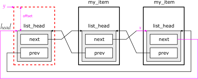
  // moving to the next item
  y = (struct my_item *)(
    (char *)x->next -
    offsetof(struct my_item,
             link)
    );
  // testing, if it is head
  if (head != &y->link) ...
  

  Figure 6: An illustration of the Linux list data structure. The gray boxes represent the linking structure list_head that is nested into a user-defined structure my_item, whose instances the user needs to be linked into a list. List-manipulating functions know nothing about the user-defined structures: they work with the linking structures only. The user data are accessible through pointer arithmetic only. Note that the head node of the list does not have the user-defined envelope. The code shown on the right illustrates how the list is traversed. Note also that when one passes from the last element pointed by x to its successor (hence back to the head), the involved pointer arithmetic causes that the pointer y will be pointing out of the allocated space, which is, however, correct since it will never be dereferenced (just used for further pointer arithmetic).

• Linux-list-2 is a variation on the above case. It contains functions for an initialisation of a Linux list, inserting elements at its tail, and for deleting the elements. The top-level function initializes the list, inserts several elements, traverses the elements one by one, and deletes them. Note that the sets of functions present in Linux-list-1 and Linux-list-2 have a non-empty intersection but are incomparable.

• Linux-list-2-err is a variation on Linux-list-2 where one of the inserted elements is not deleted and hence a memory leak is caused.

• Linux-list-all contains the entire collection of functions defined for working with Linux lists without any top-level function. The collection includes functions for different kinds of insertion of elements, removal of elements, swapping of elements (both within a list and between lists), moving to the end or to another list, rotation, splicing, etc. We can see that Broom produced complete contracts for many more of the functions. The contracts from Infer often do not cover cases of lists of length 0 or 1. In one of the remaining cases, Infer produced no result; and for the last one, it produced a partial result (that appears not to cover one of the branches of the function).

• intrusive-list is the intrusive list library. See Fig. 7 for an illustration how the data structure and the code looks like. Apart from features seen already above (pointer arithmetic and a need to deal with linking fields embedded into larger structures with a need to apply block splitting), the code contains also bit-masking. In particular, one bit of the next pointers is used to mark pointers back to the head node, thus effectively marking the “end” of the circular list. A further intricacy of the code is that the insertion into the list touches three nodes that may be different but that may also collapse into a single node. In the case of the Linux list, we have mentioned a similar situation but with two nodes only. Having three nodes that possibly collapse is not only beyond the capabilities of Infer but also Broom if it is used with its basic abduction strategy. This is the reason why some of the contracts produced by Broom are also not complete in this case (e.g., effectively allowing insertion into a list with more than one node only). We will, however, show below that Broom can resolve the problem when using more power of the alias-weak/alias-strong rules, though for the price of quite increased runtime requirements. As for Infer, it is clearly visible that its coverage of the functions is much weaker (interestingly, we noticed that it completely ignored the bit-masking when deriving some of the contracts).

  

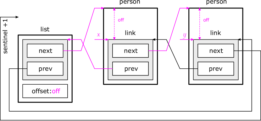
  // offset from a node pointer
  // to a link structure
  size_t off = (size_t) x -
    ((size_t)x->prev->next & ~1);
  // link of the next node
  y = (link *)(
    (size_t)lnk->next & ~1 + off
    );
  

  Figure 7: An illustration of the intrusive list data structure. The code fragment shown to the right of the figure gives the code used in the function link_get_next to obtain the linking structure of the next node. Note the use of the pointer arithmetic including bit-masking (to clear the bit whose bit-masking on the next pointers is used to denote the sentinel node of the list).

• intrusive-list-min contains a subset of the functions considered above (for initializing a list, inserting an element, removing an element) together with a top-level function utilising these functions. Essentially, the intention here was to create an as small as possible example of the given kind already problematic for Infer. Again, even Broom cannot handle it fully under its standard abduction strategy.

• intrusive-list-smoke contains the entire intrusive list library from above together with several top-level functions provided by the author to test the library. The tests use structures modelling some personal records to be linked into a list via the embedded linking structures. They create a few such records, link them into a list, traverse them (forward/backward), and destroy the list.

We now proceed to our experiments with the alias-weak/alias-strong rules. As we have said above, these rules involve a lot of guessing. Hence, if they are used to explore various possible abduction solutions based on different aliasing scenarios, the running time may grow considerably, but it may resolve situations that are otherwise not resolved. To confirm this, we have applied Broom with the strategy of using the alias-weak/alias-strong rules to explore different possible abduction solutions with different possible aliasing scenarios on the intrusive list case study. The results are shown in Table 2. The first row concerns the experiment intrusive-list-min discussed already above. At that time, we noted that Broom could not fully handle some of the intrusive list functions since they required it to merge three possibly independent nodes into a single one. As can be seen in Table 2, with the help of the alias-weak/alias-strong rules, Broom does fully manage even this problem (though the runtime grew a lot). The next two rows—intrusive-list-min-2 and intrusive-list-min-3—are variations on the previous case where we intentionally introduced some bugs, which were correctly discovered. Finally, the last row shows a significant improvement even for the entire library of intrusive lists together with its “smoke” tests.

Table 2: Experiments with alias-weak/alias-strong in Broom

Name	Expected result	Fncs total	T [m]	Funcs contr	Res
intrusive-list-min	no error	9	46	9	no error found
intrusive-list-min-2	memory leak	9	47	9	memory leak
intrusive-list-min-3	double free	9	49	9	double free
intrusive-list-smoke	no error	20	505	16	no error found

To sum up, we believe that, despite the highly prototypical nature of Broom, the presented experiments show that the proposed approach is indeed capable of handling code that is beyond the capabilities of other currently existing approaches.

9 Conclusion and Future Works

We have presented a new SL-based bi-abduction analysis capable of analysing fragments of code that manipulates with various forms of dynamic linked lists implemented using advanced low-level pointer operations. This includes operations such as pointer arithmetic, bit-masking on pointers, block operations, dealing with blocks of in-advance-unknown size, splitting them into fields of not-fixed size, which can then be merged again, etc. Although our approach builds on a body of previous research, especially, [2, 6, 7, 16], it extends it significantly to handle the mentioned features. In particular, to be able to handle the considered kind of code, we build on a flavor of SL that uses a per-field separating conjunction instead of a per-object separating conjunction, and we also introduce a number of new abduction rules that allow us to deal with pointer arithmetic, block splitting and merging, and so on. We have implemented the proposed approach in a prototype tool Broom. Despite Broom is a very early prototype, our experiments with it allowed us to handle code fragments that are—to the best of our knowledge—out of the capabilities of currently existing analysers.

We believe that there is a lot of space for further improvements of our results in the future. First, we would like to significantly optimize Broom to make it applicable to larger code bases. Here, we are thinking of applying many of the low-level optimisations applied in other tools of a similar kind (replacing as many as possible of SMT queries by answering them using simple static rules, using incremental SMT solving, caching as much information as possible, etc.). Next, we would like to explore possibilities how to reduce the amount of non-determinism present in the abduction when the alias-weak/strong rules are applied. The goal is to preserve as much as possible of the power of these rules but reduce the cost of applying them. Perhaps, we could rely here partially on some pre-defined heuristics and partially even on some techniques from machine learning, which are now being applied even in SMT solvers and elsewhere. Next, we would like to significantly improve our implementation of list abstractions (inspired, e.g., by [16]) as well as numerical abstractions. Last but not least, we would also like to think of adding support for other classes of dynamic data structures than lists.

Appendix A An Illustration of the Analysis of Conditions and Loops

When the code of a function contains conditional branching, one splits the computation for each particular branch, leading to a set of $\{({\rm Phys.\leavevmode\nobreak\ Rev.\leavevmode\nobreak\ E}_{i},Q_{i})\}$ pairs at the end of the function. When all the ${\rm Phys.\leavevmode\nobreak\ Rev.\leavevmode\nobreak\ E}_{i}$ are mutually disjoint (i.e. the branching is determined by the precondition), one can use directly all the thus obtained contracts. This is illustrated by the analysis of the function $a$ in Fig. 8. Note that the analysis leads to two contracts for the function $a$ determined by the value of the parameter $x$.

struct sll { struct sll *next;};

struct sll *a(struct sll *x) {

1. 1. $({\rm Phys.\leavevmode\nobreak\ Rev.\leavevmode\nobreak\ E}\equiv x=X,\quad Q\equiv x=X)$

2. if (x == NULL) {

   1. $\ \ \ \ ({\rm Phys.\leavevmode\nobreak\ Rev.\leavevmode\nobreak\ E}\equiv X=\mathsf{null}*x=X,\quad Q\equiv X=\mathsf{null}*x=X)$

3. struct sll *y = malloc(sizeof(struct sll));

   1. $\ \ \ \ ({\rm Phys.\leavevmode\nobreak\ Rev.\leavevmode\nobreak\ E}\equiv X=\mathsf{null}*x=X,\quad Q\equiv\exists Y.\ Y\mapsto\top[8]*\mathfrak{b}(Y)=Y*X=\mathsf{null}*x=X*y=Y)$

4. y–>next = NULL;

   1. $\ \ \ \ ({\rm Phys.\leavevmode\nobreak\ Rev.\leavevmode\nobreak\ E}\equiv X=\mathsf{null}*x=X,\quad Q\equiv\exists Y.\ Y\mapsto 0[8]*\mathfrak{b}(Y)=Y*X=\mathsf{null}*x=X*y=Y)$

5. x = y;

   1. $\ \ \ \ ({\rm Phys.\leavevmode\nobreak\ Rev.\leavevmode\nobreak\ E}\equiv X=\mathsf{null}*x=X,\quad Q\equiv\exists Y.\ Y\mapsto 0[8]*\mathfrak{b}(Y)=Y*X=\mathsf{null}*x=y=Y)$

6. }

   1. $({\rm Phys.\leavevmode\nobreak\ Rev.\leavevmode\nobreak\ E}_{1}\equiv X\neq\mathsf{null}*x=X,\quad Q_{1}\equiv X\neq\mathsf{null}*x=X)$

   1. $({\rm Phys.\leavevmode\nobreak\ Rev.\leavevmode\nobreak\ E}_{2}\equiv X=\mathsf{null}*x=X,\quad Q_{2}\equiv\exists Y.\ Y\mapsto 0[8]*\mathfrak{b}(Y)=Y*X=\mathsf{null}*x=y=Y)$

7. return x;

} summary:

1. $({\rm Phys.\leavevmode\nobreak\ Rev.\leavevmode\nobreak\ E}_{1}\equiv X\neq\mathsf{null}*x=X,\quad Q_{1}\equiv X\neq\mathsf{null}*ret=x=X)\\ ({\rm Phys.\leavevmode\nobreak\ Rev.\leavevmode\nobreak\ E}_{2}\equiv X=\mathsf{null}*x=X,\quad Q_{2}\equiv\exists Y.\ Y\mapsto 0[8]*\mathfrak{b}(Y)=Y*X=\mathsf{null}*ret=x=Y)$

Figure 8: An illustration of the analysis of a deterministic condition

For an illustration of how a loop is analysed, see Fig. 9. When analysing a loop, branching is encountered whenever the computation reaches the loop header. For instance, in the example, starting from $({\rm Phys.\leavevmode\nobreak\ Rev.\leavevmode\nobreak\ E}_{11},Q_{11})$, one continues inside the loop with $({\rm Phys.\leavevmode\nobreak\ Rev.\leavevmode\nobreak\ E}_{21},Q_{21})$ and out of the loop with $({\rm Phys.\leavevmode\nobreak\ Rev.\leavevmode\nobreak\ E}_{41},Q_{41})$. At the end of the loop, the analysis returns to the location corresponding to the loop header, which is a part of the set of the control-flow cut-points. Therefore one checks whether the current pre-/post-pair is covered by some so-far computed one related to the loop header. If no, the abstraction is run, and the new pair is added to those so-far computed for the loop header. In particular, the pair $({\rm Phys.\leavevmode\nobreak\ Rev.\leavevmode\nobreak\ E}_{32},Q_{32})$ is not covered, and so we add $({\rm Phys.\leavevmode\nobreak\ Rev.\leavevmode\nobreak\ E}_{32}^{\alpha},Q_{32}^{\alpha})$ to the line corresponding to the loop header. When the pair is covered by another one, the analysis discards the pair. For example, $({\rm Phys.\leavevmode\nobreak\ Rev.\leavevmode\nobreak\ E}_{33},Q_{33})$ is covered by $({\rm Phys.\leavevmode\nobreak\ Rev.\leavevmode\nobreak\ E}_{13},Q_{13})$ because $(\exists L2,L3.{\rm Phys.\leavevmode\nobreak\ Rev.\leavevmode\nobreak\ E}_{33})\models(\exists L_{2}.{\rm Phys.\leavevmode\nobreak\ Rev.\leavevmode\nobreak\ E}_{13})$ and $(\exists L2,L3.Q_{33})\models(\exists L_{2}.Q_{13})$. For all the contract candidates at the end of the loop, one has to use the second analysis phase to prove that the abstraction applied on the precondition did not introduce any bad configuration into the precondition.

struct sll { struct sll *next;};

struct sll *loop(struct sll *x) {

1. 1. $({\rm Phys.\leavevmode\nobreak\ Rev.\leavevmode\nobreak\ E}_{11}\equiv x=X,\quad Q_{11}\equiv x=X)$

   1. $({\rm Phys.\leavevmode\nobreak\ Rev.\leavevmode\nobreak\ E}_{12}\equiv X\mapsto l_{1}*x=X,\quad Q_{12}\equiv X\mapsto L_{1}*x=L_{1})$

   1. $({\rm Phys.\leavevmode\nobreak\ Rev.\leavevmode\nobreak\ E}_{13}\equiv\operatorname{\mathsf{ls}}(X,L_{2})*x=X,\quad Q_{13}\equiv\operatorname{\mathsf{ls}}(X,L_{2})*x=L_{2})$

2. while (x != NULL) {

   1. $\ \ \ \ ({\rm Phys.\leavevmode\nobreak\ Rev.\leavevmode\nobreak\ E}_{21}\equiv X\neq\mathsf{null}*x=X,\quad Q_{21}:X\neq\mathsf{null}*x=X)$

   1. $\ \ \ \ ({\rm Phys.\leavevmode\nobreak\ Rev.\leavevmode\nobreak\ E}_{22}\equiv X\mapsto L_{1}*L_{1}\neq\mathsf{null},\quad Q_{22}\equiv X\mapsto L_{1}*L_{1}\neq\mathsf{null}*x=L_{1})$

   1. $\ \ \ \ ({\rm Phys.\leavevmode\nobreak\ Rev.\leavevmode\nobreak\ E}_{23}\equiv\operatorname{\mathsf{ls}}(X,L_{2})*L_{2}\neq\mathsf{null}*x=X,\quad Q_{23}\equiv\operatorname{\mathsf{ls}}(X,L_{2})*L_{2}\neq\mathsf{null}*x=L_{2})$

3. x = x–>next;

   1. $\ \ \ \ ({\rm Phys.\leavevmode\nobreak\ Rev.\leavevmode\nobreak\ E}_{31}\equiv X\mapsto L_{1}*x=X,\quad Q_{31}\equiv X\mapsto L_{1}*x=L_{1})$

   1. $\ \ \ \ ({\rm Phys.\leavevmode\nobreak\ Rev.\leavevmode\nobreak\ E}_{32}\equiv X\rightarrow L_{1}*L_{1}\mapsto L_{2}*x=X,\quad Q_{32}\equiv X\mapsto L_{1}*L_{1}\mapsto L_{2}*x=L_{2})$

   1. $\ \ \ \ ({\rm Phys.\leavevmode\nobreak\ Rev.\leavevmode\nobreak\ E}_{32}^{\alpha}\equiv\operatorname{\mathsf{ls}}(X,l_{2})*x=X,\quad Q_{32}^{\alpha}\equiv\operatorname{\mathsf{ls}}(X,L_{2})*x=L_{2})$

   1. $\ \ \ \ ({\rm Phys.\leavevmode\nobreak\ Rev.\leavevmode\nobreak\ E}_{33}\equiv\operatorname{\mathsf{ls}}(X,L_{2})*L_{2}\mapsto L_{3}*x=X,\quad Q_{33}\equiv\operatorname{\mathsf{ls}}(X,L_{2})*L_{2}\mapsto L_{3}*x=L_{3})$

   1. discard state: $({\rm Phys.\leavevmode\nobreak\ Rev.\leavevmode\nobreak\ E}_{33},Q_{33})$—entailment $(\exists L_{3}.{\rm Phys.\leavevmode\nobreak\ Rev.\leavevmode\nobreak\ E}_{33})\models(\exists L_{2}.{\rm Phys.\leavevmode\nobreak\ Rev.\leavevmode\nobreak\ E}_{13})$ and $(\exists L_{3}.Q_{33})\models(\exists L_{2}.Q_{13})$

4. }

   1. $({\rm Phys.\leavevmode\nobreak\ Rev.\leavevmode\nobreak\ E}_{41}\equiv X=\mathsf{null}*x=X,\quad Q_{41}\equiv X=\mathsf{null}*x=X)$

   1. $({\rm Phys.\leavevmode\nobreak\ Rev.\leavevmode\nobreak\ E}_{42}\equiv X\mapsto L_{1}*L_{1}=\mathsf{null}*x=X,\quad Q_{42}\equiv X\mapsto L_{1}*x=L_{1}=\mathsf{null})$

   1. $({\rm Phys.\leavevmode\nobreak\ Rev.\leavevmode\nobreak\ E}_{43}\equiv\operatorname{\mathsf{ls}}(X,L_{2})*L_{2}=\mathsf{null}*x=X,\quad Q_{43}\equiv\operatorname{\mathsf{ls}}(X,L_{2})*x=L_{2}=\mathsf{null})$

5. …

}

Figure 9: An illustration of the analysis of a loop

Finally, we provide in Fig. 10 an illustration of how the analysis deals with non-deterministic branching—plus we also illustrate the use of the two analysis phases. The function $f$ from Fig. 10 has an if-statement with a non-deterministic condition, which is translated to two outgoing control-flow edges that are not labelled by any condition in our modelling. The analysis of the then branch leads to the candidate precondition ${\rm Phys.\leavevmode\nobreak\ Rev.\leavevmode\nobreak\ E}_{1}\equiv X\mapsto L*x=X$. The analysis of the else branch leads to the candidate precondition ${\rm Phys.\leavevmode\nobreak\ Rev.\leavevmode\nobreak\ E}_{2}\equiv x=X$. Then, we run the second phase which can be done in a quite similar way as the first phase. However, whenever we need to strengthen the precondition, we immediately stop with a failure. The computation first starts with the pair $({\rm Phys.\leavevmode\nobreak\ Rev.\leavevmode\nobreak\ E}_{1},{\rm Phys.\leavevmode\nobreak\ Rev.\leavevmode\nobreak\ E}_{1})$, and we compute two postconditions $Q_{11}$ and $Q_{12}$. Therefore, the final contract is $({\rm Phys.\leavevmode\nobreak\ Rev.\leavevmode\nobreak\ E}_{1},Q_{11}\vee Q_{12})$. Then we start the second phase from $({\rm Phys.\leavevmode\nobreak\ Rev.\leavevmode\nobreak\ E}_{2},{\rm Phys.\leavevmode\nobreak\ Rev.\leavevmode\nobreak\ E}_{2})$, but we realize that the precondition is not safe enough to execute all possible branches of the function—we realize that we need to infer a stronger one by using the learn-finish abduction rule. Therefore we drop ${\rm Phys.\leavevmode\nobreak\ Rev.\leavevmode\nobreak\ E}_{2}$.

struct sll { struct sll *next;};

// The first analysis phase

struct item *f(struct item *x) {

1. 1. $({\rm Phys.\leavevmode\nobreak\ Rev.\leavevmode\nobreak\ E}\equiv x=X,\quad Q\equiv x=X)$

2. if (random())

   1. $\ \ \ \ ({\rm Phys.\leavevmode\nobreak\ Rev.\leavevmode\nobreak\ E}\equiv x=X,\quad Q\equiv x=X)$

3. return x–>next;

   1. $\ \ \ \ ({\rm Phys.\leavevmode\nobreak\ Rev.\leavevmode\nobreak\ E}\equiv X\mapsto L*x=X,\quad Q\equiv X\mapsto L*ret=L*x=X)$

4. else

   1. $\ \ \ \ ({\rm Phys.\leavevmode\nobreak\ Rev.\leavevmode\nobreak\ E}\equiv x=X,\quad Q\equiv x=X)$

5. return x;

   1. $\ \ \ \ ({\rm Phys.\leavevmode\nobreak\ Rev.\leavevmode\nobreak\ E}\equiv x=X,\quad Q\equiv ret=x=X)$

} candidate preconditions:

1. ${\rm Phys.\leavevmode\nobreak\ Rev.\leavevmode\nobreak\ E}_{1}\equiv X\mapsto L*x=X\\ {\rm Phys.\leavevmode\nobreak\ Rev.\leavevmode\nobreak\ E}_{2}\equiv x=X$

// The second analysis phase

struct item *f(struct item *x) {

1. 1. $({\rm Phys.\leavevmode\nobreak\ Rev.\leavevmode\nobreak\ E}_{1}\equiv X\mapsto L*x=X,\quad Q_{1}\equiv X\mapsto L*x=X)$

   1. $({\rm Phys.\leavevmode\nobreak\ Rev.\leavevmode\nobreak\ E}_{2}\equiv x=X,\quad Q_{2}\equiv x=X)$

2. if (random())

   1. $\ \ \ \ ({\rm Phys.\leavevmode\nobreak\ Rev.\leavevmode\nobreak\ E}_{1}\equiv X\mapsto L*x=X,\quad Q_{1}\equiv X\mapsto L*x=X)$

   1. $\ \ \ \ ({\rm Phys.\leavevmode\nobreak\ Rev.\leavevmode\nobreak\ E}_{2}\equiv x=X,\quad Q_{2}\equiv x=X)$

3. return x–>next;

   1. $\ \ \ \ ({\rm Phys.\leavevmode\nobreak\ Rev.\leavevmode\nobreak\ E}_{1}\equiv X\mapsto L*x=X,\quad Q_{1}\equiv X\mapsto L*ret=L*x=X)$

   1. $\ \ \ \ ({\rm Phys.\leavevmode\nobreak\ Rev.\leavevmode\nobreak\ E}_{2}\equiv{\color[rgb]{1,0,0}X\mapsto L}*x=X,\quad Q_{2}\equiv X\mapsto L*ret=L*x=X)$

   1. discard state: $({\rm Phys.\leavevmode\nobreak\ Rev.\leavevmode\nobreak\ E}_{2},Q_{2})$ because we should learn a missing part of the precondition $X\mapsto L$

4. else

   1. $\ \ \ \ ({\rm Phys.\leavevmode\nobreak\ Rev.\leavevmode\nobreak\ E}_{1}\equiv X\mapsto L*x=X,\quad Q_{1}\equiv X\mapsto L*x=X)$

5. return x;

   1. $\ \ \ \ ({\rm Phys.\leavevmode\nobreak\ Rev.\leavevmode\nobreak\ E}_{1}\equiv X\mapsto L*x=X,\quad Q_{1}\equiv X\mapsto L*ret=x=X)$

} summary:

1. $({\rm Phys.\leavevmode\nobreak\ Rev.\leavevmode\nobreak\ E}_{11}\equiv X\mapsto L*x=X,\quad Q_{11}\equiv X\mapsto L*ret=L*x=X)\\ ({\rm Phys.\leavevmode\nobreak\ Rev.\leavevmode\nobreak\ E}_{12}\equiv X\mapsto L*x=X,\quad Q_{12}\equiv X\mapsto L*ret=x=X)$

Figure 10: An illustration of the analysis of a non-deterministic condition

Appendix B An Illustration of Bit-masking and Pointer Arithmentics

The Figure 11 containes an additional example taken from our intrusive-list experiment (see Section 8.4). This example uses a (i) bit-masking to mark an first node in the circular doubly-linked list and (ii) pointer arithmetic.

struct link { struct link *prev; void *next; };

struct link *link_get_next(struct link *l) {

1. 1. ${\rm Phys.\leavevmode\nobreak\ Rev.\leavevmode\nobreak\ E}\equiv l=L,\quad Q\equiv l=L$

2. struct link *a = l–>prev;

   1. ${\rm Phys.\leavevmode\nobreak\ Rev.\leavevmode\nobreak\ E}\equiv L\mapsto A*l=L,\\ Q\equiv L\mapsto A*l=L*a=A$

3. void *b = a–>next;

   1. ${\rm Phys.\leavevmode\nobreak\ Rev.\leavevmode\nobreak\ E}\equiv L\mapsto A*A+8\mapsto B*l=L,\\ Q\equiv L\mapsto A*A+8\mapsto B*l=L*a=A*b=B$

4. size_t c = (size_t) b & $\sim$1;

   1. ${\rm Phys.\leavevmode\nobreak\ Rev.\leavevmode\nobreak\ E}\equiv L\mapsto A*A+8\mapsto B*l=L,\\ Q\equiv\exists C.\ L\mapsto A*A+8\mapsto B*C=B\leavevmode\nobreak\ \&\leavevmode\nobreak\$-2$\leavevmode\nobreak\ *\leavevmode\nobreak\ l=L*a=A*b=B*c=C$

5. size_t o = (size_t) l - c; // offset from a node pointer to a link structure

   1. ${\rm Phys.\leavevmode\nobreak\ Rev.\leavevmode\nobreak\ E}\equiv L\mapsto A*A+8\mapsto B*l=L,\\ Q\equiv\exists C,O.\ L\mapsto A*A+8\mapsto B*C=B\leavevmode\nobreak\ \&\leavevmode\nobreak\$-2$\leavevmode\nobreak\ *\leavevmode\nobreak\ O=L-C*l=L*a=A*b=B*c=C*o=O$

6. void *d = (size_t) l–>next;

   1. ${\rm Phys.\leavevmode\nobreak\ Rev.\leavevmode\nobreak\ E}\equiv L\mapsto A*L+8\mapsto D*A+8\mapsto B*l=L,\\ Q\equiv\exists C,O.\ L\mapsto A*L+8\mapsto D*A+8\mapsto B*C=B\leavevmode\nobreak\ \&\leavevmode\nobreak\$-2$\leavevmode\nobreak\ *\leavevmode\nobreak\ O=L-C*l=L*a=A*\\ b=B*c=C*o=O*d=D$

7. size_t f = (size_t) d & $\sim$1; // link field for the next node

   1. ${\rm Phys.\leavevmode\nobreak\ Rev.\leavevmode\nobreak\ E}\equiv L\mapsto A*L+8\mapsto D*A+8\mapsto B*l=L,\\ Q\equiv\exists C,F,O.\ L\mapsto A*L+8\mapsto D*A+8\mapsto B*C=B\leavevmode\nobreak\ \&\leavevmode\nobreak\$-2$\leavevmode\nobreak\ *\leavevmode\nobreak\ O=L-C*\\ F=D\leavevmode\nobreak\ \&\leavevmode\nobreak\$-2$\leavevmode\nobreak\ *\leavevmode\nobreak\ l=L*a=A*b=B*c=C*o=O*d=D*f=F$

8. size_t e = f + o;

   1. ${\rm Phys.\leavevmode\nobreak\ Rev.\leavevmode\nobreak\ E}\equiv L\mapsto A*L+8\mapsto D*A+8\mapsto B*l=L,\\ Q\equiv\exists C,E,F,O.\ L\mapsto A*L+8\mapsto D*A+8\mapsto B*C=B\leavevmode\nobreak\ \&\leavevmode\nobreak\$-2$\leavevmode\nobreak\ *\leavevmode\nobreak\ O=L-C*\\ F=D\leavevmode\nobreak\ \&\leavevmode\nobreak\$-2$\leavevmode\nobreak\ *\leavevmode\nobreak\ E=F+O\leavevmode\nobreak\ *\leavevmode\nobreak\ l=L*a=A*b=B*c=C*o=O*d=D*f=F*e=E$

9. return (struct link *) e;

   1. ${\rm Phys.\leavevmode\nobreak\ Rev.\leavevmode\nobreak\ E}\equiv L\mapsto A*L+8\mapsto D*A+8\mapsto B*l=L,\\ Q\equiv\exists C,E,F,O.\ L\mapsto A*L+8\mapsto D*A+8\mapsto B*C=B\leavevmode\nobreak\ \&\leavevmode\nobreak\$-2$\leavevmode\nobreak\ *\leavevmode\nobreak\ O=L-C*\\ F=D\leavevmode\nobreak\ \&\leavevmode\nobreak\$-2$\leavevmode\nobreak\ *\leavevmode\nobreak\ E=F+O\leavevmode\nobreak\ *\leavevmode\nobreak\ l=L*a=A*b=B*c=C*o=O*d=D*f=F*ret=e=E$

} summary:

1. ${\rm Phys.\leavevmode\nobreak\ Rev.\leavevmode\nobreak\ E}\equiv L\mapsto A*L+8\mapsto D*A+8\mapsto B*l=L,\\ Q\equiv\exists C,E,F,O.\ L\mapsto A*L+8\mapsto D*A+8\mapsto B*C=B\leavevmode\nobreak\ \&\leavevmode\nobreak\$-2$\leavevmode\nobreak\ *\leavevmode\nobreak\ O=L-C*\\ F=D\leavevmode\nobreak\ \&\leavevmode\nobreak\$-2$\leavevmode\nobreak\ *\leavevmode\nobreak\ E=F+O\leavevmode\nobreak\ *\leavevmode\nobreak\ l=L*ret=E$

Figure 11: An illustrative example of a code from Fig. 7 using pointer arithmetic and bit-masking

References

- [1] Andrew W. Appel. Program Logics - for Certified Compilers. Cambridge University Press, 2014.
- [2] J. Berdine, C. Calcagno, B. Cook, D. Distefano, P.W. O’Hearn, T. Wies, and H. Yang. Shape Analysis for Composite Data Structures. In Proc. of CAV’07, volume 4590 of LNCS. Springer, 2007.
- [3] A. Bouajjani, C. Drăgoi, C. Enea, and M. Sighireanu. Accurate Invariant Checking for Programs Manipulating Lists and Arrays with Infinite Data. In Proc. of ATVA’12, volume 7561 of LNCS. Springer, 2012.
- [4] C. Calcagno and D. Distefano. Infer: An Automatic Program Verifier for Memory Safety of C Programs. In Proc. of NFM’11, volume 6617 of LNCS. Springer, 2011.
- [5] C. Calcagno, D. Distefano, P. O’Hearn, and H. Yang. Beyond Reachability: Shape Abstraction in the Presence of Pointer Arithmetic. In Proc. of SAS’06, volume 4134 of LNCS. Springer, 2006.
- [6] C. Calcagno, D. Distefano, P. O’Hearn, and H. Yang. Compositional Shape Analysis by Means of Bi-Abduction. In Proc. of POPL’09. ACM, 2009.
- [7] C. Calcagno, D. Distefano, P. O’Hearn, and H. Yang. Compositional Shape Analysis by Means of Bi-Abduction. Journal of the ACM, 58(6), 2011.
- [8] Cristiano Calcagno, Peter W. O’Hearn, and Hongseok Yang. Local action and abstract separation logic. In LICS, pages 366–378. IEEE Computer Society, 2007.
- [9] B.-Y.E. Chang, X. Rival, and G.C. Necula. Shape Analysis with Structural Invariant Checkers. In Proc. of SAS’07, volume 4634 of LNCS. Springer, 2007.
- [10] W.-N. Chin, C. David, H.H. Nguyen, and S. Qin. Automated Verification of Shape, Size and Bag Properties via User-defined Predicates in Separation Logic. Science of Computer Programming, 77(9), 2012.
- [11] C. Curry, Q. Loc Le, and S. Qin. Bi-Abductive Inference for Shape and Ordering Properties. In Proc. of ICECCS’19. IEEE, 2019.
- [12] L.M. de Moura and N. Bjørner. Z3: An Efficient SMT Solver. In Proc. of TACAS’08, volume 4963 of LNCS. Springer, 2008.
- [13] Stéphane Demri, Étienne Lozes, and Alessio Mansutti. The effects of adding reachability predicates in propositional separation logic. In FoSSaCS, volume 10803 of Lecture Notes in Computer Science, pages 476–493. Springer, 2018.
- [14] C. Drăgoi, C. Enea, and M. Sighireanu. Local Shape Analysis for Overlaid Data Structures. In Proc. of SAS’13, volume 7935 of LNCS. Springer, 2013.
- [15] K. Dudka, P. Peringer, and T. Vojnar. An Easy to Use Infrastructure for Building Static Analysis Tools. In Proc. of EUROCAST’11, volume 6927 of LNCS. Springer, 2011.
- [16] K. Dudka, P. Peringer, and T. Vojnar. Byte-Precise Verification of Low-Level List Manipulation. In Proc. of SAS’13, volume 7935 of LNCS. Springer, 2013.
- [17] M. Echenim, R. Iosif, and N. Peltier. Unifying Decidable Entailments in Separation Logic with Inductive Definitions. In Proc. of CADE’21, volume 12699 of LNCS. Springer, 2021.
- [18] C. Enea, O. Lengál, M. Sighireanu, and T. Vojnar. Compositional Entailment Checking for a Fragment of Separation Logic. In Proc. of APLAS’14, volume 8858 of LNCS. Springer, 2014.
- [19] B. Fang and M. Sighireanu. Hierarchical Shape Abstraction for Analysis of Free List Memory Allocators. In Proc. of LOPSTR’16, volume 10184 of LNCS. Springer, 2016.
- [20] J. Heinen, T. Noll, and S. Rieger. Juggrnaut: Graph Grammar Abstraction for Unbounded Heap Structures. In Proc. of TSS’09, volume 266 of ENTCS. Elsevier, 2010.
- [21] L. Holík, O. Lengál, J. Šimáček, A. Rogalewicz, and T. Vojnar. Fully Automated Shape Analysis Based on Forest Automata. In Proc. of CAV’13, volume 8044 of LNCS. Springer, 2013.
- [22] R. Iosif, A. Rogalewicz, and T. Vojnar. Deciding Entailments in Inductive Separation Logic with Tree Automata. In Proc. of ATVA’14, volume 8837 of LNCS. Springer, 2014.
- [23] S. Ishtiaq and P.W. O’Hearn. Separation and Information Hiding. In Proc. of POPL’01. ACM, 2001.
- [24] J.L. Jensen, M.E. Jørgensen, M.I. Schwartzbach, and N. Klarlund. Automatic Verification of Pointer Programs Using Monadic Second-order Logic. In Proc. of PLDI’97. ACM, 1997.
- [25] J. Katelaan and F. Zuleger. Beyond Symbolic Heaps: Deciding Separation Logic With Inductive Definitions. In Proc. of LPAR’11, volume 73 of EPiC Series in Computing. EasyChair, 2020.
- [26] Q. Loc Le. Compositional Satisfiability Solving in Separation Logic. In Proc. of VMCAI’21, volume 12597 of LNCS. Springer, 2021.
- [27] Q. Loc Le, C. Gherghina, S. Qin, and W.-N. Chin. Shape Analysis via Second-Order Bi-Abduction. In Proc. of CAV’14, volume 8559 of LNCS. Springer, 2014.
- [28] P. Maksimovic, S.-É. Ayoun, J.F. Santos, and P. Gardner. Gillian, Part II: Real-World Verification for JavaScript and C. In Proc. of CAV’21, volume 12760 of LNCS. Springer, 2021.
- [29] P. Maksimovic, J.F. Santos, S.-É. Ayoun, and P. Gardner. Gillian: A Multi-Language Platform for Unified Symbolic Analysis. Technical Report arXiv:2105.14769, arXiv.org, 2021.
- [30] V. Malik, M. Hruška, P. Schrammel, and T. Vojnar. Template-Based Verification of Heap-Manipulating Programs. In Proc. of FMCAD’18. IEEE, 2018.
- [31] Jens Pagel and Florian Zuleger. Strong-separation logic. In ESOP, volume 12648 of Lecture Notes in Computer Science, pages 664–692. Springer, 2021.
- [32] J.C. Reynolds. Separation Logic: A Logic for Shared Mutable Data Structures. In Proc. of LICS’02. IEEE, 2002.
- [33] M. Sagiv, T. Reps, and R. Wilhelm. Parametric Shape Analysis via 3-Valued Logic. ACM Transactions on Programming Languages and Systems, 24(3), 2002.
- [34] J.F. Santos, P. Maksimovic, S.-É. Ayoun, and P. Gardner. Gillian: Compositional Symbolic Execution for All. Technical Report arXiv:2001.05059, arXiv.org, 2020.
- [35] J.F. Santos, P. Maksimovic, S.-É. Ayoun, and P. Gardner. Gillian, Part I: A Multi-Language Platform for Symbolic Execution. In Proc. of PLDI’20. ACM, 2020.
- [36] T. Wies, V. Kuncak, K. Zee, A. Podelski, and M. Rinard. On Verifying Complex Properties using Symbolic Shape Analysis. In Proc. of HAV’07, 2007.
- [37] H. Yang, O. Lee, J. Berdine, C. Calcagno, B. Cook, D. Distefano, and P.W. O’Hearn. Scalable Shape Analysis for Systems Code. In Proc. of CAV’08, volume 5123 of LNCS. Springer, 2008.
- [38] K. Zee, V. Kuncak, and M.C. Rinard. Full Functional Verification of Linked Data Structures. In Proc. of PLDI’08. ACM, 2008.