Generation of gravitational waves from freely decaying turbulence

Abstract

We study the stochastic gravitational wave background (SGWB) produced by freely decaying vortical turbulence in the early Universe. We thoroughly investigate the time correlation of the velocity field, and hence of the anisotropic stresses producing the gravitational waves. With hydrodynamical simulations, we show that the unequal time correlation function (UETC) of the Fourier components of the velocity field is Gaussian in the time difference, as predicted by the ”sweeping” decorrelation model. We introduce a decorrelation model that can be extended to wavelengths around the integral scale of the flow. Supplemented with the evolution laws of the kinetic energy and of the integral scale, this provides a new model UETC of the turbulent velocity field consistent with the simulations. We discuss the UETC as a positive definite kernel, and propose to use the Gibbs kernel for the velocity UETC as a natural way to ensure positive definiteness of the SGWB. The SGWB is given by a 4-dimensional integration of the resulting anisotropic stress UETC with the gravitational wave Green’s function. We perform this integration using a Monte Carlo algorithm based on importance sampling, and find that the result matches that of the simulations. Furthermore, the SGWB obtained from the numerical integration and from the simulations show close agreement with a model in which the source is constant in time and abruptly turns off after a few eddy turnover times. Based on this assumption, we provide an approximate analytical form for the SGWB spectrum and its scaling with the initial kinetic energy and integral scale. Finally, we use our model and numerical integration algorithm to show that including an initial growth phase for the turbulent flow heavily influences the spectral shape of the SGWB. This highlights the importance of a complete understanding of the turbulence generation mechanism.

1 Introduction

Gravitational wave (GW) signals from the early Universe have the potential to provide a new observational perspective on high energy physics phenomena. In this context, first order cosmological phase transitions provide a compelling source of GWs. This was first proposed many years ago (see Refs. [1, 2, 3, 4, 5, 6]), before it became clear that the electroweak (EW) symmetry breaking proceeds as a crossover in the Standard Model [7]. However, it has since emerged that many scenarios beyond the Standard Model (BSM) lead to first order phase transitions at – and beyond – the EW scale, reopening the case for the study of GW production from first order phase transitions (for a GW-oriented review, see Ref. [8]).

This is particularly interesting in the context of the Laser Interferometer Space Antenna (LISA), which is sensitive to a frequency window in the millihertz range [9]. In the context of primordial GW-sourcing processes that are localized in time, such as a first order phase transition, the characteristic frequency of the GWs today can be connected to the characteristic time/length scale of the source anisotropic stresses $L_{*}$, via

$$f\simeq 16.5\cdot 10^{-3}\,\mathrm{mHz}\,\frac{1}{L_{*}\mathcal{H}_{*}}\frac{T_{*}}{100\,\mathrm{GeV}}\left(\frac{g_{*}}{100}\right)^{1/6}.$$ (1.1)

Here a subscript $*$ denotes the epoch at which the phase transition occurs. This shows that LISA can potentially detect the GW signal from transitions in the window 100 GeV – 1 TeV, if the characteristic time/length scale of the anisotropic stresses is of the order $L_{*}\sim 10^{-2}$ to $10^{-3}$ of the Hubble scale $\mathcal{H}_{*}^{-1}$ at the time of the phase transition. These can be considered as typical values for $L_{*}\mathcal{H}_{*}$, given that $L_{*}$ is related to the mean bubble separation $R_{*}$ (see e.g. [10, 8] and references therein). LISA will therefore offer a new way to probe BSM physics, complementary to the Large Hadron Collider (see e.g. Ref. [11]).

There are several processes possibly leading to sizable anisotropic stresses in connection with a first order phase transition. This rich phenomenology renders phase transitions particularly appealing as primordial GW sources. Bubble percolation, with the consequent breaking of spherical symmetry, is the most direct one [3, 4, 5]. The GW generation by bubble collision has been analysed both with simulations [12, 13, 14, 15, 16, 17, 18, 19] and analytical approaches [20, 21, 22].

The first 3-dimensional (3D) simulations of the coupled system of a scalar field and a relativistic fluid have shown that sound waves, produced in the fluid by expanding bubbles, are also a promising source of GWs [23, 24, 25]. These simulations have been performed using the code SCOTTS (Simulations of COsmic Thermal TransitionS) on which we will also rely in the present work. Analytical insight into the generation of GWs by sound waves has been developed in Refs. [26, 27], and a new simulation technique for computing the GW spectra in the sound shell limit has been proposed in Ref. [28].

Refs. [23, 24, 25] performed simulations of first order phase transitions of weak to intermediate strength, e.g. $\alpha\lesssim 0.1$, where $\alpha$ is the ratio of the trace anomaly of the energy momentum tensor and the thermal energy. It was found that the bulk fluid motion consisted primarily of compressional modes, which correspond to sound waves. In this case, sound waves are expected to be the dominant GW source. However, shocks will develop in the fluid and are expected to convert the acoustic phase into a turbulent one [29, 30]. The characteristic time of shock formation can be estimated as $\tau_{\mathrm{sh}}\sim R_{*}/\overline{v}_{\parallel}$, where $\overline{v}_{\parallel}$ denotes the root-mean-squared (rms) velocity of the acoustic motion. For stronger transitions, in which the initial value of $\overline{v}_{\parallel}$ is typically larger, the onset of turbulence is expected to occur earlier and give a more substantial contribution to the total GW signal. Furthermore, recent simulations of transitions with $\alpha\sim 0.5$ found that, if the bubble wall velocity is subsonic, flows with substantial vorticity are already generated during the transition itself when fluid shells and bubble walls collide [31].

In the present work, we study the GW signal generated by a hypothetical turbulent phase in the aftermath of a first order phase transition. The first analyses of the GW signal from turbulence have relied on analytical modelling of the turbulent flow, and semi-analytical estimates of the GW signal [6, 32, 33, 34, 35, 36, 37]. In particular, Ref. [38] evaluates the GW signal from all components (compressional, vortical, magnetic field) of both standard, and helical, freely-decaying magneto-hydrodynamic (MHD) turbulence. Various spectral shapes and scalings of the GW power spectrum per logarithmic wave number interval have been found, depending on the relative amplitude of the compressional and vortical components, and on the presence of helicity. In Ref. [38], it was also argued that the correct auto-correlation time to be used in the equations describing GW production by turbulence is the Eulerian eddy turnover time (see Ref. [39]). Far in the inertial range, the Eulerian eddy turnover time becomes $\tau_{E}(k)\sim(kv_{\mathrm{sw}})^{-1}$, where $v_{\mathrm{sw}}\simeq\overline{v}/3$ is a locally uniform velocity field sweeping the vortices, in accordance with the Kraichnan random sweeping approximation [40], and $\overline{v}$ is the rms velocity of the turbulence. Earlier work used the Lagrangian eddy turnover time $\tau_{\ell}(k)\sim(kv_{\ell})^{-1}$, where $v_{\ell}$ denotes the characteristic velocity on the scale $\ell\sim 1/k$ [33, 34, 36]. Our simulations confirm that the Eulerian eddy turnover time is the correct option.

Simulations of both non-helical and helical MHD turbulence and the resulting GW generation have been carried out in Refs. [41, 42, 43, 44]. In these works there is an initial phase in which the MHD turbulence develops, starting from a nearly monochromatic electromotive force, or a kinetic forcing. They find that the spectral shape of the GW signal varies, depending on whether a fully-developed turbulent magnetic and/or velocity field is present in the initial conditions, or whether it is sourced by the forcing.

In this paper, we develop a semi-analytical model of GW generation by freely-decaying kinetic, vortical, non-helical turbulence, which we support with the results of simulations. We rely on the relativistic hydrodynamic code SCOTTS, developed by the authors of Refs. [23, 24, 25, 31], but we use it to study the evolution of vortical fluid motion, excluding the dynamics of the scalar field undergoing the transition (see Section 5). We have chosen to over-simplify the turbulence model (no compressional modes, no helicity, no magnetic field, no initial forcing phase) in order to have full control of our analytical understanding of the GW production. Inclusion of these additional features will be tackled in future works.

The layout of the paper is as follows. We begin with a short review of stochastic gravitational wave backgrounds in the context of vortical turbulence in Section 2. We first introduce the equations of motion for the metric perturbations in an FLRW background, and write their solutions in terms of Green’s functions and the anisotropic shear stress. The gravitational wave energy density power spectrum in the radiation era is then constructed, assuming a statistically homogeneous and isotropic signal. The solution for the gravitational wave energy density power spectrum is given in terms of an integral over the Green’s function and the unequal time correlator (UETC) of the anisotropic stress. The section concludes by reviewing the computation of the anisotropic stress UETC in the context of vortical turbulence, decomposing the anisotropic stress UETC into a kernel which contains the fluid velocity UETC.

We continue by modelling freely decaying turbulence in Section 3. In Section 3.1, we introduce the velocity power spectrum for a divergence free velocity field, along with important quantities such as the integral scale of the flow $\xi$, and the rms velocity $\overline{v}$. In our modelling, we assume that the turbulent flow is described by a von Kármán spectrum, which has a Kolmogorov power law in the inertial range and a causal slope of $k^{5}$ at large scales, where $k$ refers to the power spectrum wavenumber. The evolution of the velocity field in decaying turbulence is considered in Section 3.2. Here we review the self-similarity properties of the turbulent power spectrum, starting from dimensional arguments and the assumption that there is a single length scale in the flow. On further assuming that the eddy turnover time, $\tau_{\xi}$, is the only principal timescale in the flow, one arrives at exponential decay laws for the kinetic energy and integral scale, where the decay exponents of both quantities are in principle related. We conclude with Section 3.3, where we introduce a model for the velocity UETC. To model the decorrelation in time, we follow Ref. [38] and adopt the exponential decorrelation provided by the short-time analysis of Ref. [39]. This consistently reproduces the random sweeping model [40] in the inertial range, which is supported by numerical works simulating decaying isotropic turbulence (see e.g. Ref. [45]).

In Section 4 we expand on the discussion of UETCs by considering them in the context of positive kernels and Mercer’s condition. Indeed, any two-point correlation function of a random variable satisfies a set of inequalities known as Mercer’s condition. Positive kernels are defined as the functions satisfying Mercer’s condition, thus they are candidates to model UETCs. Earlier works, such as Ref. [36], encountered the question of how to define a valid correlation function for a non-stationary process. Here, we consistently address this issue in the context of the theory of positive kernels, and propose to model the unequal time correlator (UETC) of the turbulent velocity field as a Gibbs Kernel. This provides a way to symmetrize the unequal time correlator and, most importantly, it guarantees that the anisotropic stress two-point function is a valid correlation function. As a consequence, this leads to a GW energy density power spectrum which is always positive, as it should be.

After discussing the theory, we move on to describe our simulations in Section 5. We introduce the Minkowski space simulation code, SCOTTS, and discuss how it has been modified to study relativistic vortical turbulence. To prepare the initial conditions, we initialize the velocity field in momentum space, where each mode is randomly drawn using Gaussian statistics from a von Kármán power spectrum. We also project the velocity field so that it is purely vortical. After outlining our suite of simulation runs, we specify the methodology for outputting the velocity power spectra and UETC, as well as the procedure for evolving the metric perturbations and obtaining the gravitational wave power spectrum in the simulations.

In the following two sections we present our results. First, we focus on the evolution of the velocity field in the simulations, in Section 6. We study the evolution of the kinetic energy and of the integral scale of the flow in Section 6.1, and link it to the model of Section 3.2. In the simulations, the velocity power spectrum displays self-similar scaling towards the end of the simulation, but the theoretical relation between the decay law exponents and the velocity spectrum power law at large scales is not satisfied. We also test our model for the velocity UETC in Section 6.2. The combination of the Gibbs Kernel model of the UETC with the decorrelation of Ref. [39] performs well for both the inertial range and for large scale modes. We compare our model to that of Ref. [38], and find that our model has a closer agreement with the simulation data.

Our results for the gravitational wave power spectrum are given in Section 7. There are three different cases. We begin by evaluating the gravitational wave power spectrum under the assumption that the turbulence is stationary, in Section 7.1. Next we cover the case of instantaneously generated turbulence in Section 7.2, which contains our main results regarding the SGWB spectrum. Here our initial conditions are a fully developed turbulent power spectrum. We first show the SGWB extracted from the simulations. We then calculate the gravitational wave signal using our model of freely decaying turbulence outlined in Sections 3 and 4. In this case, to calculate the gravitational wave power spectrum, we use Monte Carlo integration with importance sampling to compute the integrals found in Section 2. Using this technique, we confirm that the precise values of the decay law exponents are unimportant for the final spectral shape. We also describe the constant source approximation, in which the source of gravitational waves is taken to be constant in time, before it is turned off abruptly [46]. We obtain in this context a ready-to-use formula for the SGWB spectrum from hydrodynamic turbulence. We compare the gravitational wave power spectrum under all of these methods, finding good agreement in their mutual regions of applicability. The final case we consider in Section 7.3 is the inclusion of a simplified turbulence growth phase. Using our turbulence model and Monte Carlo integration, we calculate the gravitational wave power spectrum in the case of linear growth for both a $\mathcal{C}^{0}$ and a $\mathcal{C}^{1}$ growth phase. The inclusion of a growth phase substantially affects the shape of the gravitational wave power spectrum, underlining the importance of studying the creation mechanism of turbulence in the early Universe. Finally, we summarize our results and conclusions in Section 8.

To help the reader, in Table 1 we summarize some timescales and temporal parameters which appear in different sections of this paper.

Simulations (SCOTTS code) (Section 5)
time variable	description	properties
$\tau_{*}$	initial time in the simulation
$\tau_{\mathrm{end}}$	final time in the simulation	$k(\tau_{\mathrm{end}}-\tau_{*})\gtrsim 10$
$\tau_{\mathrm{ref}}$	reference time at which UETCs measured	$\tau_{*}<\tau_{\mathrm{ref}}<\tau_{\mathrm{end}}$

Semi-analytical evaluation of GW spectrum (Section 7)
time variable	description	properties
$\tau_{\mathrm{ini}}$	initial integration time	turbulence starts
$\tau_{\mathrm{gro}}$	timescale over which turbulence is sourced (see Section 7.3)
$\tau_{*}$	start of turbulence free decay	$\tau_{*}=\tau_{\mathrm{ini}}+\tau_{\mathrm{gro}}\equiv\mathcal{H}_{*}^{-1}$
$\tau_{\xi_{*}}$	initial eddy turnover time	$\tau_{\xi_{*}}=\xi_{*}/\overline{v}_{*}$
$\mathcal{N}_{\mathrm{e}}$	characteristic decay time of the source in units of $\tau_{\xi_{*}}$	dimensionless, $\order{1}$
$\mathcal{N}_{\mathrm{cut}}$	duration of the source in units of $\tau_{\xi_{*}}$ (used in the stationary source approximation of Section 7.1, and in the constant source approximation of Section 7.2.3)	dimensionless, $\order{1}$

Table 1: Important timescales and temporal parameters used in this article. A $*$ subscript indicates quantities evaluated at $\tau_{*}$. In the above, $k$ refers to the magnitude of the non-zero wavenumbers on the discrete momentum space lattice in the simulations.

2 Stochastic background of gravitational waves from vortical turbulence

2.1 Generation of gravitational waves

In the cosmological context, GWs are described by transverse and traceless tensor spatial perturbations $h_{ij}$ of the background FLRW metric for a homogeneous and isotropic Universe:

$$\differential{s}^{2}=a^{2}(\tau)\quantity[-\differential{\tau}^{2}+(\delta_{ij}+2h_{ij})\differential{x}^{i}\differential{x}^{j}],$$ (2.1)

with $\partial_{i}h_{ij}=h_{ii}=0$. Here $a(\tau)$ is the scale factor, and $\tau$ the conformal time. It follows from the linearized Einstein equations that $h_{ij}\quantity(\mathbf{k},\tau)$ satisfies

$$\ddot{h}_{ij}+2\mathcal{H}\dot{h}_{ij}+k^{2}h_{ij}=8\pi Ga^{2}(\tau)\Pi^{(TT)}_{ij}\quantity(\mathbf{k},\tau)$$ (2.2)

where $\mathcal{H}=\dot{a}/{a}$ is the comoving Hubble parameter, $\cdot=\derivative*{\tau}$, $\mathbf{k}$ denotes a comoving wave-vector, and $\Pi_{ij}^{(TT)}$ is the transverse traceless part of the anisotropic stress tensor. The anisotropic stress is defined by

$$\Pi_{ij}=T_{ij}-p(\delta_{ij}+2h_{ij})\text{,}$$ (2.3)

with $T_{\mu\nu}$ the fluid energy momentum tensor, and $p$ its pressure. The transverse traceless component of the anisotropic stress is extracted by means of the projector

$$\Pi_{ij}^{(TT)}(\mathbf{k},\tau) =\Lambda_{ij\ell m}(\hat{\mathbf{k}})\Pi_{\ell m}(\mathbf{k},\tau),$$ (2.4)

$$\text{with}~{}~{}\Lambda_{ij\ell m}(\hat{\mathbf{k}}) =\bot_{i\ell}(\hat{\mathbf{k}})\bot_{jm}(\hat{\mathbf{k}})-\frac{1}{2}\bot_{ij}(\hat{\mathbf{k}})\bot_{\ell m}(\hat{\mathbf{k}})\text{,}$$ (2.5)

$$\text{and}~{}~{}\bot_{ij}(\hat{\mathbf{k}}) =\delta_{ij}-\hat{k}_{i}\hat{k}_{j}\text{.}$$ (2.6)

We work in the radiation era, and therefore we further define $\Pi_{ij}^{(TT)}=(4\rho/3)\tilde{\Pi}_{ij}$ with $\rho$ the energy density in the early, radiation dominated Universe, and $p=\rho/3$. Using Friedmann’s equation, Eq. 2.2 can be rewritten as

$$\ddot{h}_{ij}+2\mathcal{H}\dot{h}_{ij}+k^{2}h_{ij}=4\mathcal{H}^{2}\tilde{\Pi}_{ij}\quantity(\mathbf{k},\tau).$$ (2.7)

Assuming that there were no changes in the relativistic degrees of freedom, $\mathcal{H}=\tau^{-1}$, and changing variable from $h_{ij}(\mathbf{k},\tau)$ to $\tau h_{ij}(\mathbf{k},\tau)$, Eq. 2.7 becomes the equation for a forced harmonic oscillator whose Green’s function is known (see Ref. [47] for a review). The solution and its time derivative are

$$h_{ij}\quantity(\mathbf{k},\tau) =4\int_{\tau_{\mathrm{ini}}}^{\tau}\frac{\differential\zeta}{\zeta}\frac{\sin k(\tau-\zeta)}{k\tau}\tilde{\Pi}_{ij}(\mathbf{k},\zeta),$$ (2.8)

$$\dot{h}_{ij}\quantity(\mathbf{k},\tau) =4\int_{\tau_{\mathrm{ini}}}^{\tau}\frac{\differential\zeta}{\zeta}\quantity[\frac{\cos k(\tau-\zeta)}{\tau}-\frac{\sin k(\tau-\zeta)}{k\tau^{2}}]\tilde{\Pi}_{ij}(\mathbf{k},\zeta).$$ (2.9)

where $\tau_{\mathrm{ini}}$ is the conformal time at which the source turns on.

2.2 GW energy density power spectrum

We assume that the GWs are generated by a stochastic process (specifically vortical turbulence) and consist of signals coming from patches in the sky that were causally disconnected at the moment of their emission in the very early Universe. Assuming statistical homogeneity and isotropy, the two-point correlation function of $\dot{h}_{ij}$ can be written as

$$\expectationvalue{\dot{h}^{*}_{ij}(\mathbf{k},\tau)\dot{h}_{ij}(\mathbf{q},\tau)}\equiv(2\pi)^{3}\delta(\mathbf{q}-\mathbf{k})P_{\dot{h}}(k,\tau),$$ (2.10)

which defines the spectral density $P_{\dot{h}}$. The fractional GW energy density power spectrum at conformal time $\tau$ in the radiation era is then

$$\evaluated{\derivative{\Omega_{\mathrm{gw}}}{\ln k}}_{\tau}=\frac{k^{3}P_{\dot{h}}(k,\tau)}{2(2\pi)^{3}Ga^{2}(\tau)\rho(\tau)}.$$ (2.11)

The relevant statistical object of the GW source is the unequal time correlation function (UETC) of the anisotropic stress, defined by

$$\expectationvalue{\tilde{\Pi}_{ij}(\mathbf{k},\tau)\tilde{\Pi}^{*}_{ij}(\mathbf{q},\zeta)}\equiv(2\pi)^{3}\delta(\mathbf{k-q})P_{\tilde{\Pi}}(k,\tau,\zeta).$$ (2.12)

From Eq. 2.9, one then obtains

$$P_{\dot{h}}(k,\tau)=\frac{16}{\tau^{2}}\iint_{\tau_{\mathrm{ini}}}^{\tau}\frac{\differential{\eta}}{\eta}\frac{\differential{\zeta}}{\zeta}\,\mathcal{G}(k,\tau,\eta,\zeta)P_{\tilde{\Pi}}(k,\eta,\zeta),$$ (2.13)

with

$$\mathcal{G}(k,\tau,\eta,\zeta)=\cos k(\tau-\eta)\cos k(\tau-\zeta)-2\frac{\cos k(\tau-\eta)\sin k(\tau-\zeta)}{k\tau}+\frac{\sin k(\tau-\eta)\sin k(\tau-\zeta)}{(k\tau)^{2}}\,.$$ (2.14)

The GW energy density fraction Eq. 2.11 becomes then

$$\evaluated{\derivative{\Omega_{\mathrm{gw}}}{\ln k}}_{\tau}=\frac{8}{3\pi^{2}}k^{3}\iint_{\tau_{\mathrm{ini}}}^{\tau}\mathcal{G}(k,\tau,\eta,\zeta)P_{\tilde{\Pi}}(k,\eta,\zeta)\frac{\differential{\eta}}{\eta}\frac{\differential{\zeta}}{\zeta},$$ (2.15)

where we have used the Friedmann equation $3\mathcal{H}^{2}=8a^{2}\pi G\rho$. As can be appreciated from Eq. 2.15, the GW signal is sourced by the UETC of the anisotropic stress energy of the turbulent fluid, $P_{\tilde{\Pi}}(k,\tau,\zeta)$.

2.3 The unequal time anisotropic stress correlator

We now review the computation of the UETC of the turbulent fluid anisotropic stress, defined in Eq. 2.12. The starting point is the spatial, off-diagonal part of the energy momentum tensor of a relativistic fluid. In order to simplify the computation, we neglect the spatial dependence of the fluid enthalpy density, and set the Lorentz factor $\gamma=1$. This amounts to assuming non-relativistic turbulence. As we shall see, we find an excellent agreement between the semi-analytical results based on the non-relativistic source model and the relativistic simulations, also in what concerns the GW signal. Therefore, the assumption of non-relativistic turbulence does not significantly affect our final results, within the tested range of initial rms velocity. We then approximate

$$T_{ij}(\mathbf{x},\tau)\approx(\rho+p)v_{i}(\mathbf{x},\tau)v_{j}(\mathbf{x},\tau),\quad\text{for }i\neq j.$$ (2.16)

On using Eqs. 2.3 and 2.4, the two point correlation of the normalized anisotropic stress becomes

$$\expectationvalue{\tilde{\Pi}_{ij}(\mathbf{k},\tau)\tilde{\Pi}^{*}_{ij}(\mathbf{k^{\prime}},\zeta)}=\\ \Lambda_{ij\ell m}(\hat{\mathbf{k}})\Lambda_{ijrs}(\hat{\mathbf{k^{\prime}}})\int\frac{\differential[3]{p}}{(2\pi)^{3}}\frac{\differential[3]{h}}{(2\pi)^{3}}\expectationvalue{v_{\ell}(\mathbf{p},\tau)v_{m}(\mathbf{k-p},\tau)v_{r}^{*}(\mathbf{h},\zeta)v_{s}^{*}(\mathbf{k^{\prime}-h},\zeta)}.$$ (2.17)

We assume Gaussianity of the velocity field to rewrite the four-point velocity correlator in terms of two-point correlators using Wick’s theorem:

$$\begin{split}\expectationvalue{\tilde{\Pi}_{ij}(\mathbf{k},\tau)\tilde{\Pi}^{*}_{ij}(\mathbf{k^{\prime}},\zeta)}=&\Lambda_{ij\ell m}(\hat{\mathbf{k}})\Lambda_{ijrs}(\hat{\mathbf{k^{\prime}}})\int\frac{\differential[3]{p}}{(2\pi)^{3}}\frac{\differential[3]{h}}{(2\pi)^{3}}\\ &\quad[\expectationvalue{v_{\ell}(\mathbf{p},\tau)v_{m}(\mathbf{k-p},\tau)}\expectationvalue{v_{r}^{*}(\mathbf{h},\zeta)v_{s}^{*}(\mathbf{k^{\prime}-h},\zeta)}\\ &\qquad+\expectationvalue{v_{\ell}(\mathbf{p},\tau)v_{r}^{*}(\mathbf{h},\zeta)}\expectationvalue{v_{m}(\mathbf{k-p},\tau)v_{s}^{*}(\mathbf{k^{\prime}-h},\zeta)}\\ &\qquad+\expectationvalue{v_{\ell}(\mathbf{p},\tau)v_{s}^{*}(\mathbf{k^{\prime}-h},\zeta}\expectationvalue{v_{m}(\mathbf{k-p},\tau)v_{r}^{*}(\mathbf{h},\zeta)}].\end{split}$$ (2.18)

Similarly to the anisotropic stress UETC of Eq. 2.12, we can define the turbulent velocity UETC. Under the further assumption that the velocity field is divergence-free, statistically isotropic and homogeneous, the velocity UETC is

$$\expectationvalue{v_{i}(\mathbf{k},\tau)v_{j}^{*}(\mathbf{q},\zeta)}\equiv(2\pi)^{3}\delta\quantity(\mathbf{k}-\mathbf{q})\bot_{ij}(\hat{\mathbf{k}})P_{v}(k,\tau,\zeta).$$ (2.19)

Then on using $\Lambda_{ij\ell m}(\hat{\mathbf{k}})\Lambda_{ijrs}(\hat{\mathbf{k}})=\Lambda_{\ell mrs}(\hat{\mathbf{k}})$, Eq. 2.18 becomes

$$\expectationvalue{\tilde{\Pi}_{ij}(\mathbf{k},\tau)\tilde{\Pi}^{*}_{ij}(\mathbf{k^{\prime}},\zeta)}=\\ \Lambda_{\ell mrs}(\hat{\mathbf{k}})\delta(\mathbf{k-k^{\prime}})\int\differential[3]{p}P_{v}(p,\tau,\zeta)P_{v}(q,\tau,\zeta)\quantity[\bot_{\ell r}(\hat{\mathbf{p}})\bot_{ms}(\hat{\mathbf{q}})+\bot_{\ell s}(\hat{\mathbf{p}})\bot_{mr}(\hat{\mathbf{q}})],$$ (2.20)

where $\mathbf{q}=\mathbf{k}-\mathbf{p}$ (note that the first term in Eq. 2.18 does not contribute). The contraction over indices can be carried out explicitly using Eqs. 2.4, 2.5 and 2.6,

$$2\Lambda_{\ell mrs}(\hat{\mathbf{k}})\bot_{\ell r}(\hat{\mathbf{p}})\bot_{ms}(\hat{\mathbf{q}}) =1+2\quantity[(\hat{\mathbf{k}}\dotproduct\hat{\mathbf{p}})^{2}+(\hat{\mathbf{k}}\dotproduct\hat{\mathbf{q}})^{2}]+(\hat{\mathbf{k}}\dotproduct\hat{\mathbf{p}})^{2}(\hat{\mathbf{k}}\dotproduct\hat{\mathbf{q}})^{2}$$ (2.21)

$$2\Lambda_{\ell mrs}(\hat{\mathbf{k}})\bot_{\ell s}(\hat{\mathbf{p}})\bot_{mr}(\hat{\mathbf{q}}) =1+(\hat{\mathbf{k}}\dotproduct\hat{\mathbf{p}})^{2}(\hat{\mathbf{k}}\dotproduct\hat{\mathbf{q}})^{2},$$ (2.22)

so that Eq. 2.19 becomes

$$\expectationvalue{\tilde{\Pi}_{ij}(\mathbf{k},\tau)\tilde{\Pi}^{*}_{ij}(\mathbf{k^{\prime}},\zeta)}=\\ \delta(\mathbf{k-k^{\prime}})\int\differential[3]{p}P_{v}(p,\tau,\zeta)P_{v}(q,\tau,\zeta)\quantity[1+(\hat{\mathbf{k}}\dotproduct\hat{\mathbf{p}})^{2}+(\hat{\mathbf{k}}\dotproduct\hat{\mathbf{q}})^{2}+(\hat{\mathbf{k}}\dotproduct\hat{\mathbf{p}})^{2}(\hat{\mathbf{k}}\dotproduct\mathbf{q})^{2}].$$ (2.23)

We can now extract the kernel of the anisotropic stress defined in Eq. 2.12 and obtain

$$P_{\tilde{\Pi}}(k,\tau,\zeta)=\frac{1}{(2\pi)^{3}}\int\differential[3]{p}P_{v}(p,\tau,\zeta)P_{v}(q,\tau,\zeta)\quantity[1+(\hat{\mathbf{k}}\dotproduct\hat{\mathbf{p}})^{2}]\quantity[1+(\hat{\mathbf{k}}\dotproduct\hat{\mathbf{q}})^{2}].$$ (2.24)

This result agrees with Ref. [36], but differs from Ref. [38]. The reason is that in Ref. [38], the tensor indices on the two terms in square brackets on the right-hand side of Eq. 2.20 were assumed identical, but this is not the case as can be seen explicitly in Eq. 2.21 and Eq. 2.22.

The following Sections 3 and 4 are devoted to the construction of a model for the velocity UETC $P_{v}(p,\tau,\zeta)$ in Eq. 2.24.

3 Modelling freely decaying turbulence

In this section, we provide definitions and review properties of freely decaying turbulence. This will be complemented with new theoretical input regarding positive kernels in Section 4, leading to the new velocity UETC model which we propose in this work. Our new model will be validated with relativistic, simulations in Section 6.

3.1 Velocity power spectrum

The real-space two-point correlation function of a statistically homogeneous, isotropic and divergence-free velocity field reads [48]

$$b_{ij}(\mathbf{r},\tau)=\frac{\expectationvalue{v_{i}(\mathbf{x},\tau)v_{j}(\mathbf{x}+\mathbf{r},\tau)}}{\overline{v}^{2}(\tau)}\equiv\Sigma_{t}(r,\tau)\bot_{ij}(\hat{\mathbf{r}})+\Sigma_{\ell}(r,\tau)\hat{r}_{i}\hat{r}_{j},$$ (3.1)

where $\overline{v}^{2}(\tau)\equiv\expectationvalue{v_{i}(\mathbf{x},\tau)v_{i}(\mathbf{x},\tau)}$ is the rms velocity squared, and the functions $\Sigma_{t}$ and $\Sigma_{\ell}$ represent respectively the transverse and longitudinal correlation functions. Since the velocity field is divergence-free, we have that $\partialderivative*{b_{ij}}{r_{i}}=0$ and the correlation functions are related through

$$\Sigma_{\ell}^{\prime}(r)=\frac{2}{r}[\Sigma_{t}(r)-\Sigma_{\ell}(r)].$$ (3.2)

The spectral density $P_{v}(k,\tau)$

$$\expectationvalue{v_{i}(\mathbf{k},\tau)v_{j}^{*}(\mathbf{q},\tau)}\equiv(2\pi)^{3}\delta\quantity(\mathbf{k}-\mathbf{q})\bot_{ij}(\hat{\mathbf{k}})P_{v}(k,\tau)$$ (3.3)

(comparing with Eq. 2.19, note that we denote quantities at equal time with one time variable only, for conciseness) can be expressed in terms of the correlation functions $\Sigma_{\ell}$ and $\Sigma_{t}$ by matching the Fourier transform of Eq. 3.3 and the trace of Eq. 3.1 [32]:

$$P_{v}(k,\tau)=\overline{v}^{2}(\tau)\int\differential[3]{r}\,\operatorname{e}^{i\mathbf{k}\cdot\mathbf{r}}\quantity[\Sigma_{t}(r,\tau)+\frac{1}{2}\Sigma_{\ell}(r,\tau)].$$ (3.4)

In spherical coordinates and using Eq. 3.2, this becomes

$$P_{v}(k,\tau)= \;2\pi\,\overline{v}^{2}(\tau)\int\differential{r}\quantity[r^{3}\Sigma_{\ell}^{\prime}(r,\tau)+3r^{2}\Sigma_{\ell}(r,\tau)]\frac{\sin kr}{kr}$$ (3.5)

$$= \;2\pi\,\overline{v}^{2}(\tau)\int\differential{r}\quantity[r^{3}\Sigma_{\ell}^{\prime}(r,\tau)+3r^{2}\Sigma_{\ell}(r,\tau)]\quantity[1-\frac{(kr)^{2}}{6}+\order{(kr)^{4}}].$$ (3.6)

We assume that the correlation function of Eq. 3.1 has compact support because it vanishes outside the causal horizon. As a consequence, the leading order term in Eq. 3.6 is $\evaluated{r^{3}\Sigma_{\ell}}_{0}^{\infty}=0$, and the spectral density on large scales is given by

$$P_{v}(k\rightarrow 0,\tau)=\frac{2\pi}{3}\overline{v}^{2}(\tau)k^{2}\int_{0}^{\infty}\differential{r}r^{4}\,\Sigma_{\ell}(r,\tau)+\order{(kr)^{4}}\,.$$ (3.7)

Therefore, causality in the early Universe points to Batchelor turbulence, at least on super-horizon scales [32]. The coefficient of the amplitude of the large-scale part of the spectrum in Eq. 3.7 is the Loitsyansky integral $\int\differential{r}r^{4}\Sigma_{\ell}(r)$. This quantity was conjectured to be constant in time in the absence of long-range correlations (see e.g. Ref. [48]), which would then be consistent with the causality requirement.

The power spectrum $\mathcal{P}_{v}(k)$ encodes how $\overline{v}^{2}$, or equivalently the non-relativistic kinetic energy per unit enthalpy, is distributed into the different length-scales:

$$\overline{v}^{2}(\tau)\equiv\int\frac{\differential k}{k}\mathcal{P}_{v}(k,\tau).$$ (3.8)

In our notation, it is related to the spectral density through

$$\mathcal{P}_{v}(k,\tau)=\frac{k^{3}}{\pi^{2}}P_{v}(k,\tau).$$ (3.9)

Note that the power spectrum as defined here is related to the energy spectrum $E(k,\tau)$ as defined in Ref. [48] through

$$\mathcal{P}_{v}(k,\tau)=2kE(k,\tau).$$ (3.10)

To characterize the typical length-scale of the system, we also define the integral scale $\xi$ in terms of the longitudinal correlation function, or equivalently in terms of the power spectrum

$$\xi(\tau)\equiv\int_{0}^{\infty}\differential r\,\Sigma_{\ell}(r,\tau)=\frac{\pi}{4\bar{v}^{2}}\int k^{-1}\mathcal{P}_{v}(k,\tau)\differential{\ln k}.$$ (3.11)

We use the integral scale to define dimensionless, time-dependent wavenumbers

$$K(\tau)\equiv\mathcal{A}\,k\,\xi(\tau)\,,$$ (3.12)

with $\mathcal{A}$ a normalization constant given in Eq. 3.14 below.

Concerning the shape of the velocity power spectrum, we assume in our modelling that in the inertial range it is determined by the well-known Kolmogorov $K^{-2/3}$ law [49], and on large scales by the causal $K^{5}$ slope, motivated by Eq. 3.7. These properties are captured by the von Kármán spectrum [50, 48, 36, 38]

$$\mathcal{P}_{v}\quantity(k,\tau)=\mathcal{B}\,\overline{v}^{2}(\tau)\frac{K^{5}(\tau)}{\quantity[1+K^{2}(\tau)]^{17/6}}.$$ (3.13)

The coefficients $\mathcal{A}$ and $\mathcal{B}$ are chosen to ensure that the definitions of the kinetic energy and the integral scale of Eqs. 3.8 and 3.11 are consistent:

$$\mathcal{A} \equiv\frac{55\Gamma(1/3)}{12\sqrt{\pi}\Gamma(17/6)}\approx 4.02$$ (3.14)

$$\mathcal{B} \equiv\frac{8\Gamma(17/6)}{3\sqrt{\pi}\Gamma(1/3)}\approx 0.97.$$ (3.15)

Eq. 3.13 assumes that the von Kármán spectral shape is preserved during the time evolution of the turbulent field. This power spectrum will be used for the semi-analytical evaluation of the GW signal (see Section 7.2.2): self-similarity in time is therefore an underlying assumption of the resulting GW spectra. Furthermore, Eq. 3.13 will also be used as the initial condition for our hydrodynamical simulations. The simulations will show, on the other hand, that the von Kármán spectral shape is not fully preserved by time evolution: while for $K\gtrsim 1$, a power law consistent with $K^{-2/3}$ returns after $\order{10}$ eddy turnover times, a shallower one than $K^{5}$ emerges for $K\ll 1$ (see Section 6.1). Nevertheless, the GW spectra output by the simulations, and those resulting from the semi-analytical integration, are in very good agreement in their common wavenumber $K$ region: we therefore anticipate that differences in the time evolution of the large-scale part of the turbulent spectrum do not significantly affect the final results. This is due to the fact that the production of gravitational waves is fast, as we shall see.

As a consequence of the fast GW sourcing, though, the particular choice of the initial velocity power spectrum determines the final GW spectral shape. Equation (3.13) is the only input we use for exploring the SGWB signal from decaying turbulence. Nevertheless, we are able to draw general lessons from our analysis.

3.2 Evolution of the velocity field in decaying turbulence

In this section we provide a very simplified review of the time evolution of the freely-decaying turbulent power spectrum, and of average quantities such as the kinetic energy per unit enthalpy $\overline{v}^{2}(\tau)$ and the integral scale $\xi(\tau)$.

In line with the model of Section 3.1, we assume that there is only one principal length scale in the flow, $\xi$ (see e.g. Ref. [52] for a turbulence description not satisfying this hypothesis). Since the power spectrum is dimensionless, it must generally take the form (consistently with Eq. 3.13)

$$\mathcal{P}_{v}(k,\tau)=\quantity(\frac{\overline{v}(\tau)}{\overline{v}_{*}})^{2}\,\varphi[k\xi(\tau)]\,,$$ (3.16)

where the function $\varphi(k\xi(\tau))$ must satisfy integrability conditions following Eqs. 3.8 and 3.11, and $*$ indicates quantities evaluated at the start of turbulence decay. At large scales, the absence of relevant dynamical processes implies a simple power law spectrum

$$\mathcal{P}_{v}[k\xi(\tau)\ll 1,\tau]\simeq\overline{v}^{2}(\tau)\,[k\xi(\tau)]^{\beta+1}\,,$$ (3.17)

where, for the moment, the spectral index $\beta$ is left unspecified.

Further assuming that at large scales the power spectrum is constant in time, leads to

$$\overline{v}^{2}(\tau)\xi(\tau)^{1+\beta}=\mathrm{const}\,.$$ (3.18)

Under this assumption, the self-similarity of the power spectrum takes the form [55, 58]

$$\mathcal{P}_{v}(k,\tau)=\quantity(\frac{\xi_{*}}{\xi})^{1+\beta}\varphi[k\xi(\tau)]\,.$$ (3.19)

The individual time evolution of the rms velocity and the integral scale can be derived, if we further assume that there is only one principal timescale in the flow, the eddy turnover time $\tau_{\xi}=\xi/\overline{v}$. With this assumption, one can write

$$\derivative{\overline{v}^{2}}{\tau}=-c_{v}\frac{\overline{v}^{2}}{\tau_{\xi}},$$ (3.20)

where $c_{v}$ is a constant. Together with Eq. 3.18, one can solve Eq. 3.20 to derive

$$\overline{v}^{2}(\tau)=\overline{v}_{*}^{2}\left(1+\frac{\tau-\tau_{*}}{\mathcal{N}_{\mathrm{e}}\tau_{\xi_{*}}}\right)^{-p}$$ (3.21)

$$\xi(\tau)=\xi_{*}\left(1+\frac{\tau-\tau_{*}}{\mathcal{N}_{\mathrm{e}}\tau_{\xi_{*}}}\right)^{q}\,,$$ (3.22)

where the decay exponents $p$ and $q$ take the values

$$p =\frac{2(\beta+1)}{\beta+3}$$ (3.23)

$$q=\frac{2}{\beta+3},$$ (3.24)

and $\mathcal{N}_{\mathrm{e}}$ is a constant representing the number of initial eddy turn-over times that the kinetic energy takes to decay, and the integral scale to grow. In particular $p$ and $q$ satisfy

$$p=(1+\beta)q=2(1-q)\,.$$ (3.25)

Note that this model does not predict the value of $\beta$, although consistency with the arguments of Section 3.1 would indicate $\beta=4$ as would follow from the constancy of the Loitsyansky integral. In Section 6.1 we will report on our numerical investigation of the evolution of the velocity power spectrum in the framework of the model described above.

The validity of the decay laws given in Eqs. 3.21 and 3.22, together with the actual value of the parameter $\beta$ (and consequently of the decay law exponents through Eq. 3.25), are currently open problems of the theory of turbulence. Invariance of the Navier-Stokes equations under appropriate rescaling leads to the self-similarity of the velocity power spectrum, and links the decay law exponents $p$ and $q$ to the scaling parameter [59, 60]. The scaling parameter can then be related to the slope of the initial velocity power spectrum at large scales, if one assumes that the latter also satisfies the self-similarity conditions (see e.g. Ref. [61]). In this context, an initial power spectrum leading to $\beta=4$, as motivated in Section 3.1, provides $p$ and $q$ values consistent with the classical Kolmogorov theory, namely $p=10/7$ and $q=2/7$ [62, 48] (see also [63] for a numerical result). The relation between the scaling parameter and the slope of the initial power spectrum at large scales has also been derived in the context of renormalization group analyses of the incompressible MHD equations, as holding at the fixed point [64, 65]. However, the initial velocity power spectrum does not need to necessarily satisfy either the self-similarity condition, nor does it need to exhibit power law behaviour. Relaxing these assumptions changes the prediction on the subsequent free decay model, disconnecting the value of $\beta$ from the initial conditions [56, 58]. Recently, new models of the turbulent free-decay have emerged, following which the turbulence decay is governed by the integral scale rather than by the asymptotic behaviour at large scales [52, 66, 67, 68, 69]. According to these findings there would be then no universal decay regime, since the details of the spectral shape near the peak are related to the turbulence production mechanism.

Note that in both this Section and Section 3.1 we have neglected the dissipative scales. The turbulent kinetic energy dissipates at the viscous scale $\lambda$, at which the Reynolds number is $\mathrm{Re}(\lambda)=v_{\lambda}\,\lambda\,a/\nu=1$, where $\nu$ denotes the kinematic viscosity. The viscous scale $\lambda$ increases with time, and the turbulent velocity on a given scale $2\pi/k$ goes to zero once the dissipation scale has grown to $\lambda(\tau)=2\pi/k$. Furthermore, $\lambda(\tau)$ grows faster than the integral scale $\xi(\tau)$: the turbulent inertial range is therefore fully dissipated when the two scales become equal, so that $\mathrm{Re}(\xi)=1$. As previously demonstrated [37, 36], turbulence is expected to free-decay for several Hubble times, before it is fully dissipated. For example, with the initial set of parameters $T_{*}=100~{}\mathrm{GeV}$, $\overline{v}_{*}=0.03$, $\xi_{*}\mathcal{H}_{*}=0.01$, $q=2/7$, $p=10/7$, one obtains $\mathrm{Re}(\xi)=1$ at $T_{\mathrm{fin}}\sim 0.3~{}\mathrm{GeV}$, corresponding to about $1000~{}\tau_{\xi_{*}}$. The kinetic viscosity in the early Universe is indeed extremely small: for the same initial conditions, one finds $\mathrm{Re}(\xi_{*})\sim 10^{11}$, and the inertial range spans about $8$ orders of magnitude in wavenumber. In principle, we should have inserted a cutoff at $k>2\pi/\lambda(\tau)$ in the turbulent power spectrum given in Eq. 3.13, and we should account, in the GW production, for the viscous dissipation of the kinetic energy at each scale $k$ in addition to the overall free decay described by Eqs. 3.21 and 3.22. However, as we will discuss in Section 7.2, the bulk of the GW signal is generated faster than the turbulent decay: therefore, the dynamics at the viscous scale plays no role in practice in the present analysis, and it is justified to neglect it altogether.

3.3 Unequal time correlator of the velocity field

Together with the overall free-decay, we also need to model the time decorrelation of the turbulent velocity field. This is encapsulated by the normalized velocity UETC

$$R(k,\tau,\zeta)\equiv\frac{P_{v}(k,\tau,\zeta)}{\sqrt{P_{v}(k,\tau)\,P_{v}(k,\zeta)}}.$$ (3.26)

The first model to have been developed was Kraichnan’s random sweeping approximation [40], in which the decorrelation function in the inertial range is a Gaussian in the variable $k\overline{v}|\tau-\zeta|$, for small time differences. The thinking behind the model is that modes are decorrelated by being “swept” by the large-scale flow, whose rms velocity is $\overline{v}$. This model has good numerical support in the inertial range for both stationary and decaying turbulence (see for example Refs. [70, 45, 71]). We review it in Section 3.3.1.

However, for GW production calculations, we need to model the decorrelation around the peak of the velocity power spectrum. To this end, we study — for the first time with hydrodynamical simulations — the decorrelation of the turbulent velocity field outside the inertial range, as far as possible in the low wavenumber part of the spectrum. The simulation results are presented in Section 6.2, and show that a good model is obtained by replacing the rms velocity in the Gaussian with a time and scale dependent average decorrelation velocity, based on the sweeping velocity proposed in Ref. [39], which we present in Section 3.3.2.

Furthermore, we also need to take into account the formal requirement that the UETCs (velocity and anisotropic stress) must be positive definite kernels, which is not manifest in the simple Gaussian model. This will be presented in Section 4.

3.3.1 Kraichnan random sweeping approximation

The random sweeping approximation provides an explanation for the origin of the Gaussian functional form for the decorrelation. Kraichnan’s sweeping hypothesis is based on the assumption that Fourier modes of the velocity field in the inertial range are advected without deformation by a locally uniform velocity field $\mathbf{V}$, which may be time-dependent [40]. This amounts to neglecting the non-linear terms and writing

$$\partialderivative{\mathbf{v}}{\tau}+i\quantity[\mathbf{k}\dotproduct\mathbf{V}(\tau)]\mathbf{v}\simeq 0.$$ (3.27)

Since $\mathbf{V}$ is locally uniform, the evolution of modes with different wavenumbers $\mathbf{k}$ is decoupled. The turbulent velocity field can then be explicitly integrated: from Eq. 3.27 one finds

$$\mathbf{v}(\mathbf{k},\tau)\simeq\mathbf{v}(\mathbf{k},\zeta)\exp(-i\int_{\zeta}^{\tau}\mathbf{k}\dotproduct\mathbf{V}(s)\differential{s}),$$ (3.28)

where $\zeta<\tau$. Under the assumption that the locally uniform velocity field $\mathbf{V}$ is statistically independent of the turbulent velocity field $\mathbf{v}$ at the initial time, the unequal time correlator of $\mathbf{v}$ can be expressed as

$$P_{v}(k,\tau,\zeta)\simeq P_{v}(k,\zeta)\expectationvalue{\exp(-i\int_{\zeta}^{\tau}\mathbf{k}\dotproduct\mathbf{V}(s)\differential{s})}.$$ (3.29)

The average of the exponential can be calculated assuming that its argument is a Gaussian random variable. It then follows that the velocity field decorrelates with a characteristic Gaussian law,

$$P_{v}(k,\tau,\zeta)\simeq P_{v}(k,\zeta)\exp\quantity(-\frac{1}{2}\expectationvalue{X^{2}}),$$ (3.31)

where

$$X^{2}\equiv\iint_{\zeta}^{\tau}(\mathbf{k}\dotproduct\mathbf{V}(s))(\mathbf{k}\dotproduct\mathbf{V}(s^{\prime}))\differential{s}\differential{s^{\prime}}.$$ (3.32)

This expression can be further simplified assuming that on average the locally uniform velocity has the same amplitude in the three spatial directions [40], leading to

$$P_{v}(k,\tau,\zeta)\simeq P_{v}(k,\tau)\exp\quantity[-\frac{1}{2}k^{2}v_{\mathrm{sw}}^{2}(\tau,\zeta)(\tau-\zeta)^{2}],$$ (3.33)

where $v_{\mathrm{sw}}(\tau,\zeta)$ is the average sweeping velocity which takes the form [45, 72]

$$v_{\mathrm{sw}}^{2}(\tau,\zeta)=\frac{1}{3(\tau-\zeta)^{2}}\iint_{\zeta}^{{\tau}}\expectationvalue{\mathbf{V}(s)\cdot\mathbf{V}(s^{\prime})}\differential{s}\differential{s^{\prime}}.$$ (3.34)

Kraichnan’s model assumes stationary turbulence and sets the sweeping velocity to the rms velocity divided by $\sqrt{3}$, under the hypothesis of statistical isotropy [40, 73]. Since this model has good numerical support in the inertial range [70, 45, 71], The sweeping velocity should reduce to

$$v_{\mathrm{sw}}^{2}(\tau,\tau)=C_{v}^{2}\,\frac{\overline{v}^{2}(\tau)}{3}$$ (3.35)

at equal time and in the inertial range, with $C_{v}^{2}$ a numerical factor whose value will be inferred from simulations. As presented in Section 6.2, simulations indicate $C_{v}^{2}\simeq 1$,mserving as a verification of the random sweeping approximation and of statistical isotropy.

3.3.2 Scale dependent sweeping velocity

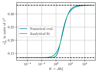
Figure 1: Extension of the decorrelation velocity at scales larger than the integral scale, following the model given in Eq. 3.36. It interpolates smoothly between $\overline{v}^{2}/3$ in the inertial range as in Eq. 3.35 and $2\overline{v}^{2}/15$ on large scales. These limits are shown with the black dashed lines.

The random sweeping approximation reviewed in Section 3.3.1 applies in the inertial range. However, in order to evaluate the GW generation, we need to model the time decorrelation of the velocity field on all scales (see for example Eq. 2.24). The decorrelation dynamics at scales larger than the integral scale in freely decaying turbulence have received little attention: numerical studies such as those performed in Refs. [45, 72], for example, study decorrelation only in the inertial range. The largest scale analysed in Ref. [70] is $k=1$, corresponding to the scale of the forcing, namely the peak of the power spectrum: it appears from this analysis that even this scale decorrelates more slowly than those of the inertial range.

In the context of the literature dedicated to GW production by turbulence, various decorrelation models have been proposed, see Refs. [33, 36, 38]. Ref. [36] assumed that the large scales do not decorrelate. The only time dependence of the velocity spectrum outside the inertial range was therefore due to the free decay, and an exponential decorrelation was inserted for wavenumbers in the inertial range by means of a step function. This introduced a non-physical discontinuity (see Eq. (57) of [36]). Furthermore, as pointed out in Ref. [38], Refs. [33, 36] used the Lagrangian eddy turnover time as typical decorrelation time, which is scale-dependent in the inertial range, and therefore in conflict with the numerical results of Refs. [70, 45].

Ref. [38] recommended the use of the model of Ref. [39], which improves Kraichnan’s random sweeping approximation by taking interactions between modes into account. The result is an Eulerian eddy turnover time which is weakly scale-dependent for wavenumbers up to $\order{10^{2}}$ times that corresponding to the integral scale. We adopt the same form for the Eulerian eddy turnover time to construct our model of the velocity UETC, but correct it to ensure the mathematical consistency of the correlation, as discussed in Section 4.

Following Refs. [74, 39], we define an instantaneous scale-dependent decorrelation velocity

$$v_{\mathrm{dc}}^{2}(k,\tau)\equiv\int_{0}^{\infty}h\quantity(\frac{q}{k})\mathcal{P}_{v}(q,\tau)\differential{\ln q},$$ (3.36)

where the function $h(x)$ is given by

$$h(x)=\frac{1}{48}(13-8x^{2}+3x^{4})+\frac{1}{32x}(1-x^{2})^{3}\ln\frac{1+x}{\absolutevalue{1-x}}.$$ (3.37)

Note that the calculations performed in Ref. [39] in principle apply only to the inertial range. We will see that extending it to lower wavenumbers is justified by the numerical data.

Eq. 3.36 reduces to $v_{\mathrm{dc}}^{2}(\tau)\simeq\overline{v}(\tau)^{2}/3$ far in the inertial range, consistent with the result of the random sweeping hypothesis, and gives $C_{v}^{2}=1$ (see Eq. 3.35). However, it also has another term, relevant at scales closer to the integral scale $\xi$, which is proportional to $-v_{k}^{2}\sim-\mathcal{P}_{v}(k)$. This negative contribution comes from the analysis at small time intervals and appears to slow down the process of decorrelation. In order to account for decorrelation at all scales, one can therefore attempt to use Eq. 3.36 as an extension of the sweeping velocity [38]. Pushing Eq. 3.36 to large scales, one can appreciate that $v_{\mathrm{dc}}(k,\tau)$ provides a continuous interpolation from $\overline{v}^{2}/3$ in the inertial range to $2\overline{v}^{2}/15$ at large scales, as shown in Fig. 1. In the semi-analytical GW evaluation, we will solve the integral of Eq. 3.36 numerically, although a good analytical fit to $v_{\mathrm{dc}}(k,\tau)$ is (we recall that $K=\mathcal{A}k\xi(\tau)$)

$$v_{\mathrm{dc}}^{2}(k,\tau)\simeq\frac{\overline{v}^{2}}{3}\quantity(\frac{1+0.2K}{\sqrt{5/2}+0.2K})^{2},$$ (3.38)

that we compare to the numerical result in Fig. 1 (note that this fit differs slightly from what was given in Ref. [38]).

In order to describe how the relevant scales in the velocity spectrum decorrelate, one might substitute, in the exponential of Eq. 3.33, the decorrelation velocity given in Eq. 3.36. This is the approach adopted in Ref. [38]. However, this breaks the time symmetry of the UETC $P_{v}(k,\tau,\zeta)$ (see Eq. 2.19). To restore this symmetry, the decorrelation velocity entering the exponential in Eq. 3.33 must depend on both times. The next section is devoted to ensuring the symmetry and positivity requirements that are necessary to model a valid UETC.

4 Unequal time correlators as positive kernels

The two-point correlation function of any random variable must be a positive kernel [75], in other words it must satisfy certain properties — most notably Mercer’s theorem. This applies to the turbulent velocity field UETC Eq. 2.19, as well as to $P_{\tilde{\Pi}}(k,\tau,\zeta)$ Eq. 2.12, describing the random anisotropic stresses arising from the turbulent field. The model of the velocity field — and consequently of the anisotropic stress — UETCs that we construct in this section ensures that they are positive kernels. According to Mercer’s theorem, this implies that the GW energy density power spectrum is indeed also positive, see Eq. 2.15. This issue had already been raised in Ref. [36], but it is analysed here in more depth directly on the velocity field UETC.

4.1 The unequal time correlation function as a non-stationary Gaussian kernel

As we have discussed in Section 3, the turbulent rms velocity and integral scale are evolving in time, while the turbulent source decorrelates. GWs are therefore generated by a non-stationary, random process, whose UETC we need to model. To do so, we make use of some general properties of two-point correlators of stochastic processes, which we review in the following.

The two-point correlator of a complex valued stochastic process $\phi(\tau)$ is defined by

$$K(\tau_{1},\tau_{2})\equiv\expectationvalue{\phi^{*}(\tau_{1})\phi(\tau_{2})}.$$ (4.1)

We assume that the real and imaginary part of the stochastic process are uncorrelated, in which case $K(\tau_{1},\tau_{2})$ is real. $K(\tau_{1},\tau_{2})$ is a positive semi-definite kernel which satisfies several properties: symmetry $K(\tau_{1},\tau_{2})=K(\tau_{2},\tau_{1})$; the Cauchy-Schwartz inequality; and the Mercer condition (see e.g. Ref. [75])

$$\iint_{I\times I}\differential{\tau_{1}}\differential{\tau_{2}}f^{*}(\tau_{1})f(\tau_{2})K(\tau_{1},\tau_{2})\geq 0\,,$$ (4.2)

for any interval $I$. This follows from the fact that, for any well-behaved function $f$, the stochastic variable $X=\int\differential{\tau}f(\tau)\phi(\tau)$ must have positive variance $\langle\absolutevalue{X}^{2}\rangle\geq 0$. One can show that the linear combination and multiplication of two kernels yield another kernel [76].

The velocity UETC $P_{v}(k,\tau,\zeta)$ is the two-point correlation function of the stochastic process $v_{i}(\mathbf{k},\tau)$ (see Eq. 2.19), and is therefore a positive semi-definite kernel. In Section 3.3 we analysed the time evolution and decorrelation properties of the velocity field, based on our understanding of the turbulence physical process. In this section, we explain how the fact that a UETC must be a positive semi-definite kernel leads to our choice of the decorrelation velocity at unequal times $v_{\mathrm{dc}}(k,\tau,\zeta)$, and how to symmetrize $P_{v}(k,\tau,\zeta)$.

The simplest example of a positive semi-definite kernel is the separable kernel $K(\tau_{1},\tau_{2})=g^{*}(\tau_{1})g(\tau_{2})$, which factorizes Mercer’s condition, Eq. 4.2, into a modulus. This type of kernel was already proposed in the context of GW generation by turbulence and primordial magnetic fields in Refs [36, 77, 37], where it is referred to as the coherent assumption. Another common form is the stationary kernel $K(\tau_{1},\tau_{2})=K(\tau_{1}-\tau_{2})$. Stationary kernels are positive if and only if there exist a positive finite function $F$ such that $K(\tau_{1}-\tau_{2})=\int\cos[\omega(\tau_{1}-\tau_{2})]F(\omega)\differential{\omega}$. From this result one can easily see that a kernel of the form $K(\tau_{1},\tau_{2})\propto\delta(\tau_{1}-\tau_{2})$ is positive definite: it is referred to as incoherent in Refs. [36, 37].

Most importantly for us, stationary kernels also include the Gaussian kernel

$$K(\tau_{1},\tau_{2})=\exp[-\alpha(\tau_{1}-\tau_{2})^{2}],$$

with $\alpha>0$, which is the form provided by the Kraichnan sweeping scenario Eq. 3.33. However, here we would like to model the power spectrum of freely decaying turbulence, which is, by definition, non-stationary. A simple but well-defined departure from stationary kernels is provided by locally stationary kernels, of the form $K(\tau_{1},\tau_{2})=K_{1}\quantity({\tau_{1}+\tau_{2}}/{2})K_{2}\quantity(\tau_{1}-\tau_{2})$, where $K_{1}$ is a non-negative function and $K_{2}$ a positive stationary kernel [78]. The UETC of a freely-decaying turbulent velocity field, though, cannot assume this form. This is because the sweeping velocity depends explicitly on time, as can be seen from Eq. 3.33. For the problem at hand, we therefore also need to go beyond local stationarity.

We do so by introducing process-convolution kernels [79]. This specific class of non-stationary kernels is defined through a two-valued complex function $g(\tau,u)$ as follows:

$$K(\tau_{1},\tau_{2})=\int g^{*}(\tau_{1},u)g(\tau_{2},u)\differential{u}.$$ (4.3)

It is easy to show that process-convolution kernels satisfy Mercer’s condition Eq. 4.2. The process-convolution kernel adapted to our case is the non-stationary Gaussian kernel, defined with the function

$$g(\tau,u)=\quantity(\frac{2}{\pi J(\tau)})^{1/4}\exp[-\frac{(\tau-u)^{2}}{J(\tau)}],$$ (4.4)

where $J(\tau)$ is a free function.

4.2 Symmetrized unequal time correlator of the velocity field

To define the kernel representing the velocity unequal time correlator, we choose for a given $k$

$$J_{k}(\tau)=\frac{1}{[k\,v_{\mathrm{dc}}(k,\tau)]^{2}},$$ (4.5)

where $v_{\mathrm{dc}}(k,\tau)$ is given in Eq. 3.36. Inserting this definition into Eq. 4.4 and further into Eq. 4.3, one finds a family of non-stationary Gaussian kernels

$$K_{k}(\tau,\zeta)=\sqrt{\frac{2\,v_{\mathrm{dc}}(k,\tau)v_{\mathrm{dc}}(k,\zeta)}{v_{\mathrm{dc}}^{2}(k,\tau)+v_{\mathrm{dc}}^{2}(k,\zeta)}}\exp[-k^{2}(\tau-\zeta)^{2}\frac{v_{\mathrm{dc}}^{2}(k,\tau)v_{\mathrm{dc}}^{2}(k,\zeta)}{v_{\mathrm{dc}}^{2}(k,\tau)+v_{\mathrm{dc}}^{2}(k,\zeta)}].$$ (4.6)

Note that these kernels satisfy $K_{k}(\tau,\tau)=1$, and are therefore of a suitable form to be used as a normalized UETC $R(k,\tau,\zeta)$.

We can now use this result to construct a UETC $P_{v}(k,\tau,\zeta)$ which satisfies the Mercer condition. First we note that the UETC evaluated at equal times is the power spectrum, $P_{v}(k,\tau,\tau)=P_{v}(k,\tau)$. Hence, multiplying the kernel Eq. 4.6 by $\sqrt{P_{v}(k,\tau)P_{v}(k,\zeta)}$ will give a function of the two times which correctly reduces to the power spectrum at equal times. This function is also a kernel, as $\sqrt{P_{v}(k,\tau)P_{v}(k,\zeta)}$ is a separable kernel, and the product of two kernels is a kernel. Our model is then

$$P_{v}\quantity(k,\tau,\zeta)=\sqrt{P_{v}(k,\tau)P_{v}(k,\zeta)}\sqrt{\frac{2v_{\mathrm{dc}}(k,\tau)v_{\mathrm{dc}}(k,\zeta)}{v_{\mathrm{dc}}^{2}(k,\tau)+v_{\mathrm{dc}}^{2}(k,\zeta)}}\exp[-\frac{1}{2}k^{2}(\tau-\zeta)^{2}v_{\mathrm{dc}}^{2}(k,\tau,\zeta)],$$ (4.7)

where the average decorrelation velocity $v_{\mathrm{dc}}(k,\tau,\zeta)$ is given by the harmonic average of the equal-time decorrelation velocity:

$$v_{\mathrm{dc}}^{2}(k,\tau,\zeta)=2\,\frac{v_{\mathrm{dc}}^{2}(k,\tau)v_{\mathrm{dc}}^{2}(k,\zeta)}{v_{\mathrm{dc}}^{2}(k,\tau)+v_{\mathrm{dc}}^{2}(k,\zeta)}.$$ (4.8)

Note that this is symmetric in the two times $\tau$ and $\zeta$.

To summarize, we have shown that the velocity UETC of Eq. 4.7 is a positive kernel, i.e. a well-defined two point correlator. This guarantees that the anisotropic stress UETC $P_{\tilde{\Pi}}(k,\tau,\zeta)$ of Eq. 2.24 is also a positive kernel, being the product of two positive kernels. Finally, the integrand of Eq. 2.15 is also a positive kernel. Indeed, $\mathcal{G}$ is a separable kernel since it results from the square of Eq. 2.9. As a consequence, the GW energy density power spectrum defined in Eq. 2.15 is always positive, as it should be.

Having managed to model the decorrelation of the freely-decaying turbulence with Eq. 4.7, we can go beyond the approach of Ref. [36]. In that paper the shear stress decorrelation was modelled directly in the anisotropic stress UETC as a top-hat function of the kind $\Theta[k\absolutevalue{\tau-\zeta}-x_{c}]$. We remark that such a function is not a positive kernel, since it is the Fourier transform of a sinc function: in order to derive a positive definite GW power spectrum, one must indeed take $x_{c}<\pi$ [36, 37].

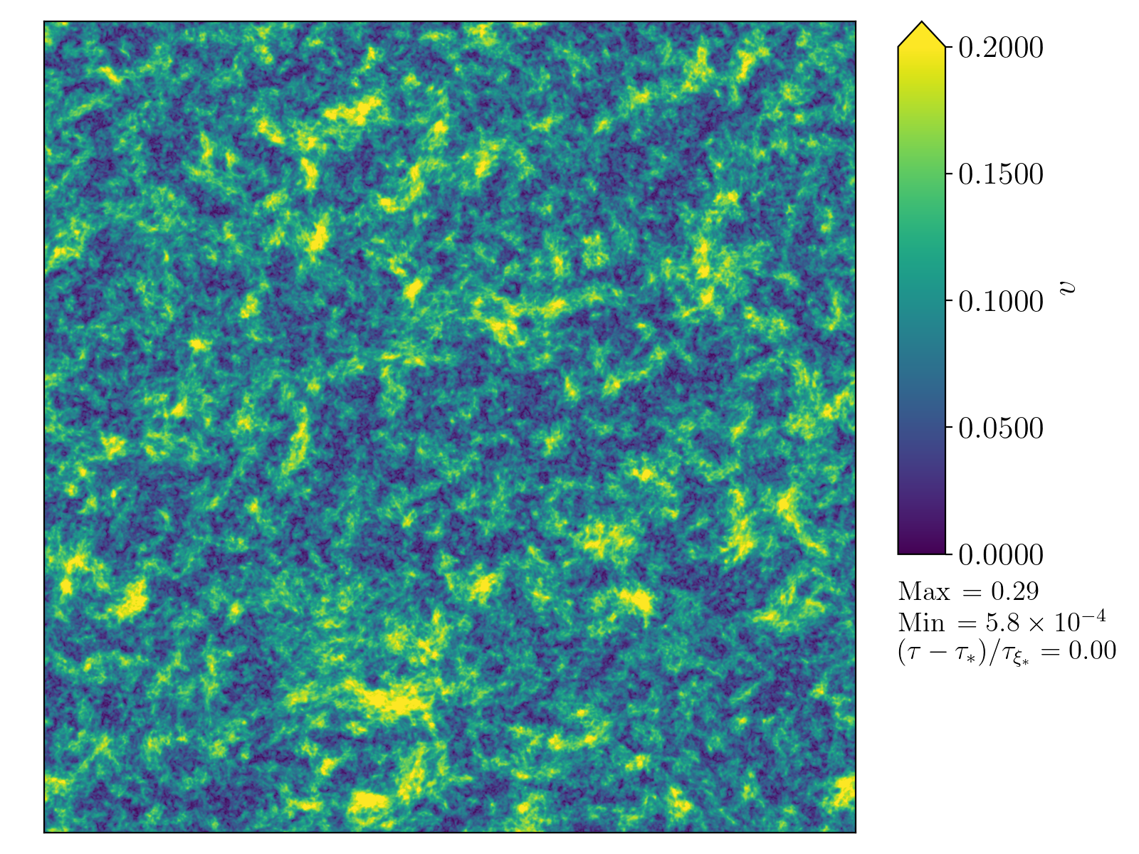
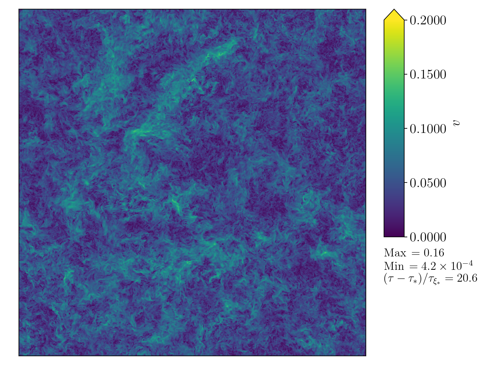
Figure 2: Left panel: Slice through simulation ($\mathrm{A}^{\prime}$) showing the velocity initial conditions in real space. Right panel: Same slice as the left panel but after a time $\Delta\tau=20.6\tau_{\xi_{*}}$ has elapsed.

5 Simulations

We carry out a series of direct hydrodynamical simulations in order to study the freely-decaying turbulent flow, in particular the UETCs of the velocity field and its overall time evolution, as well as the SGWB signal produced. For our simulations, we use a modified version of the relativistic hydrodynamics code SCOTTS, previously developed to study the coupled evolution of the scalar field and the relativistic fluid, and the production of GWs during a thermal phase transition [23, 24, 25, 31]. Here we are mainly interested in the dynamics of the fluid after the phase transition has completed. We therefore initialize the scalar field to lie in the broken phase at the start of the simulation. Given the form of the effective potential and equation of state in Ref. [31], this leaves us solely with the evolution of the relativistic fluid.

Ideally, one would want to simulate the coupled field-fluid model [80], in order to observe the generation of turbulence at all stages from the bubble collisions onwards [31]. In this work, however, we do not analyse the complete system up to fully developed turbulence. We rather concentrate on the decay of turbulence, inserting the turbulence parameters (e.g. kinetic energy and integral scale) as input values, disconnected from the rest of the phase transition dynamics. Here, we will initialize only the vortical component of the fluid velocity. This permits a cleaner analysis of the results and comparison to the semi-analytical modelling of Sections 3 and 4. We defer studying the compressional component and simulating the turbulence generation to future work. See Fig. 2 for a visualisation of the velocity field in a slice through one of our simulations at initialisation and after many eddy turnover times have passed.

In the rest of this section, we specify the equations of motion of the fluid that are solved by the code, and then explain how we fix the initial conditions and evaluate the UETCs. Finally, we discuss how we compute GW power spectra from the simulations.

5.1 Hydrodynamic evolution

Given that we are discarding the scalar field dynamics, the energy momentum tensor of the system becomes that of a perfect fluid,

$$T^{\mu\nu}=(\epsilon+p)U^{\mu}U^{\nu}+g^{\mu\nu}p\text{,}$$ (5.1)

with $\epsilon$ the internal energy density in the fluid, $p$ the pressure, $U^{\mu}=\gamma(1,\mathbf{v})$ the fluid four-velocity and with Lorentz factor $\gamma=1/\sqrt{1-v^{2}}$. The equation of state is that of an ultrarelativistic gas with $p=\epsilon/3$. It has been shown that the hydrodynamic equations of motion of an ultrarelativistic fluid in an expanding universe expressed in comoving coordinates and conformal time are the same as the hydrodynamic equations in Minkowski space-time, provided the dynamical quantities are replaced by appropriately scaled variables [81]. However, the source term for the GWs does not scale in the same way. Therefore, the Minkowski space-time code SCOTTS can be used to study hydrodynamic turbulence in an expanding background, but the output GW power spectrum can be matched to the expanding background result only for sources which are short-lived compared with the Hubble time [24].

The dynamical quantities that the code evolves are the fluid energy density $E=\gamma\epsilon$ with equation of motion [24]

$$\dot{E}+\partial_{i}(Ev^{i})+p\left[\dot{\gamma}+\partial_{i}(\gamma v^{i})\right]=0\text{,}$$ (5.2)

and the fluid momentum density $Z_{i}=\gamma^{2}(\epsilon+p)v_{i}$, the components of which evolve according to

$$\dot{Z_{i}}+\partial_{j}(Z_{i}v^{j})+\partial_{i}p=0\text{.}$$ (5.3)

The evolution algorithm follows the approach taken in Ref. [82] with a leapfrog and operator splitting approach to updating the dynamical quantities. For this work we use a van Leer scheme for the advection update [83, 84], whereas earlier uses of the SCOTTS code used an upwind donor cell scheme. For all of our simulations we pick the lattice spacing and timestep such that their ratio is $\differential x/\differential\tau=2.5$. We denote the starting time of our simulations as $\tau=\tau_{*}$. Note that while our simulations do not contain a physical viscosity, the introduction of a lattice spacing $\differential x$ effectively sets a dissipation scale. This is due to the numerical viscosity introduced by the discretization of the fluid equations. Therefore, simulations with larger $\xi_{*}/\differential x$ have a larger effective Reynolds number.

5.2 Initial conditions of the simulation

In our simulations the velocity field $\mathbf{v}$ is not necessarily divergence-free. However, as outlined in the rest of this section, we initialize the velocity field to be divergence-free in our simulations. In Appendix F we show that in this case the longitudinal component of the velocity field remains negligible throughout our simulations, and so we treat $\mathbf{v}$ as divergence-free in subsequent sections.

At the start of our simulations, we initialize the fluid energy density $E$ everywhere. For our simulations we choose to set $E\,\differential x^{4}=1/16$. Next we initialize the velocity field of the simulations in Fourier space. We do this indirectly by initializing the spatial components of the four-velocity $\mathbf{U}=\gamma\mathbf{v}$, such that

$$\mathbf{U}_{\mathbf{x}}=\frac{1}{L^{3}}\sum_{\mathbf{k}}\mathbf{U}_{\mathbf{k}}\operatorname{e}^{i\mathbf{k}\cdot\mathbf{x}},$$ (5.4)

where $\mathbf{x}$ and $\mathbf{k}$ refer to the discrete real and momentum space coordinates on the lattice, and $L^{3}$ is the total number of lattice sites. Each mode $\mathbf{U}_{\mathbf{k}}$ is randomly distributed and follows Gaussian statistics with mean zero and variance determined by the desired power spectrum serving as initial condition. Initializing $\mathbf{U}_{\mathbf{k}}$ rather than $\mathbf{v}_{\mathbf{k}}$ prevents individual modes of $\mathbf{v}_{\mathbf{k}}$ being drawn from the tails of the Gaussian with unphysical velocities larger than one. The $\mathbf{U}_{\mathbf{k}}$ field is then projected onto its vortical component with the projector $\bot_{ij}(\hat{\mathbf{k}})$, see Eq. 2.6. Since $\mathbf{U}$ is real, we impose that $\mathbf{U}_{\mathbf{k}}=\mathbf{U}^{*}_{-\mathbf{k}}$. Once the $\mathbf{U}_{\mathbf{k}}$ field is correctly initialized we perform a Fourier transform to find the real space configuration of the $\mathbf{U}$ field, and from this we can calculate the velocity field $\mathbf{v}$.

This method allows us to initialize the simulation with arbitrary choices for the $\mathbf{U}$ field power spectrum $\mathcal{P}_{U}(k,\tau)={k^{3}}P_{U}(k,\tau)/{\pi^{2}}$. Here $P_{U}(k,\tau)$ corresponds to the spectral density of the $\mathbf{U}$ field, defined via the equal time correlator (see also Eq. 3.3)

$$\langle U_{i}(\mathbf{k},\tau)U_{j}^{*}(\mathbf{q},\tau)\rangle=(2\pi)^{3}\bot_{ij}(\hat{\mathbf{k}})\delta(\mathbf{k}-\mathbf{q})P_{U}(k,\tau)\text{,}$$ (5.5)

where in our initial conditions we have set the longitudinal component of $\mathbf{U}$ to zero. We initialize the simulations with a relativistic version of the von Kármán spectrum Eq. 3.13, supplemented with a high-wavenumber cutoff:

$$\mathcal{P}_{U}(k,\tau_{*})=C\frac{(k/\tilde{k})^{5}}{[1+(k/\tilde{k})^{2}]^{17/6}}\exp\left[-\left(\frac{k}{k_{\mathrm{max}}}\right)^{2}\right]\text{.}$$ (5.6)

The two constants $\tilde{k}$ and $C$ determine respectively the peak location and amplitude. The values of $C$ and $\tilde{k}$ are chosen so that the initial rms velocity $\overline{v}_{*}=\sqrt{\overline{v}^{2}(\tau_{*})}$ (defined in Eq. 3.8) and integral scale $\xi_{*}=\xi(\tau_{*})$ (defined in Eq. 3.11) extracted from the simulation will be close to a desired value. A list of parameters for the simulations we perform is given in Table 2. In Eq. 5.6 we insert an exponential cutoff to ensure that the power does not extend to the lattice scale, with $k_{\mathrm{max}}\,\differential{x}=\pi/4$ used in our simulations.

$L^{3}$	$\overline{v}_{*}$	$\xi_{*}/\differential{x}$	$L\differential{x}/\xi_{*}$	$(\tau_{\mathrm{end}}-\tau_{*})/\tau_{\xi_{*}}$	$(\tau_{\mathrm{ref}}-\tau_{*})/\tau_{\xi_{*}}$	$\Delta\tau_{\mathrm{UETC}}/\tau_{\xi_{*}}$	C	$\tilde{k}\differential{x}$	Label
$4096^{3}$	$0.0988$	$29.8$	$138$	$99.6$	$5.97$	$1.08\,\times\,10^{-2}$	1.99	$9.19\times 10^{-3}$	(A)
$2048^{3}$	$0.0298$	$8.08$	$253$	$99.5$	$4.97$	$1.18\,\times\,10^{-3}$	0.995	$4.06\times 10^{-2}$	(B)
$2048^{3}$	$0.0274$	$57.2$	$35.8$	$12.9$	$6.47$	$9.18\,\times\,10^{-4}$	0.129	$3.28\times 10^{-3}$	(C)
$2048^{3}$	$0.0984$	$8.08$	$253$	$97.4$	$4.87$	$1.32\,\times\,10^{-2}$	0.974	$4.06\times 10^{-2}$	(D)
$2048^{3}$	$0.0955$	$64.4$	$31.8$	$11.9$	$0.594$	$1.02\,\times\,10^{-2}$	0.119	$3.28\times 10^{-3}$	(E)
$2048^{3}$	$0.279$	$8.11$	$253$	$103$	$4.13$	$1.18\,\times\,10^{-1}$	1.03	$4.06\times 10^{-2}$	(F)
$2048^{3}$	$0.289$	$70.9$	$28.9$	$11.7$	$0.466$	$9.18\,\times\,10^{-2}$	0.117	$3.28\times 10^{-3}$	(G)
$2048^{3}$	$0.0974$	$28.4$	$72.0$	$103$	$6.17$	$1.08\,\times\,10^{-2}$	2.06	$9.19\times 10^{-3}$	($\mathrm{A}^{\prime}$)
$1024^{3}$	$0.0942$	$25.4$	$40.4$	$111$	$6.69$	$1.08\,\times\,10^{-2}$	2.23	$9.19\times 10^{-3}$	($\mathrm{A}^{\prime\prime}$)

Table 2: List of the simulations used in this work. We list the number of sites in the lattice for each simulation $L^{3}$, the initial rms velocity $\overline{v}_{*}=\sqrt{\overline{v}^{2}(\tau_{*})}$ (see Eq. 3.8) and integral scale $\xi_{*}=\xi(\tau_{*})$ (see Eq. 3.11) extracted from the simulation on the initial timestep. The relative size of each simulation to the integral scale $L\differential{x}/\xi_{*}$ is given. We also list the final time of each simulation $\tau_{\mathrm{end}}$, the UETC reference time $\tau_{\mathrm{ref}}$ and the UETC output interval $\Delta\tau_{\mathrm{UETC}}$, all given in units of the eddy turnover time at the integral scale $\tau_{\xi_{*}}=\xi_{*}/\overline{v}_{*}$. Finally we list the parameters for the simulation input power spectrum as given in Eq. 5.6. Simulations ($\mathrm{A}^{\prime}$) and ($\mathrm{A}^{\prime\prime}$) are used to test the effects of finite volume and are discussed in Appendix C.

5.3 Velocity power spectra in the simulations

During the simulation we regularly output the rotational velocity power spectra $\mathcal{P}_{v}(k,\tau)$. We validate that the longitudinal piece of the velocity correlator $P_{v}(k,\tau)$ is negligible over the full duration of all our simulations, providing it is initialized to be zero, see Appendix F. To find the velocity power spectrum within our simulations, we first perform a discrete Fourier transform on the real space field to obtain the Fourier modes

$$\mathbf{v}_{\mathbf{k}}=\sum_{\mathbf{x}}\mathbf{v}_{\mathbf{x}}\operatorname{e}^{-i\mathbf{x}\cdot\mathbf{k}}\text{.}$$ (5.7)

The rotational power spectrum is then approximated by projecting and binning these modes in momentum space. The power spectrum for the $r$-th bin is constructed via

$$\mathcal{P}_{v}(k_{r},\tau)=\frac{1}{L^{6}}\frac{k_{r}}{\Delta k}\sum_{r\leq\tfrac{|\mathbf{k}|}{\Delta k}<r+1}\bot_{ij}(\mathbf{\hat{k}})v^{i}_{\mathbf{k}}(\tau){v}^{j*}_{\mathbf{k}}(\tau)\text{,}$$ (5.8)

where $k_{r}=2\pi(r+1/2)/L\differential x$ is the central value of the bin in $k$, and $\Delta k=2\pi/L\differential x$ is the bin width. Note that the power spectra from the simulation are formed from an average over a spherical shell in $\mathbf{k}$ of Fourier modes.

5.4 Unequal time correlators in the simulations

We are also interested in studying the UETCs of the velocity field in these simulations as these enable us to model the GW source, see Eqs. 2.15 and 2.24. However, evaluating $P_{v}(k,\tau,\zeta)$ for many values of $\tau$ and $\zeta$ is very costly within a simulation, in part because each pair of $\tau$ and $\zeta$ represents snapshots of the field $\mathbf{v}$ that must be stored concurrently in memory. Instead, we define a reference time $\tau_{\mathrm{ref}}$ at which we store in memory the field $\mathbf{v}(\mathbf{k},\tau_{\mathrm{ref}})$, and then compute the UETC at regular intervals with the field on the current timestep, i.e.

$$\expectationvalue{v_{i}(\mathbf{k},\tau)v_{j}^{*}(\mathbf{q},\tau_{\mathrm{ref}})}=(2\pi)^{3}\bot_{ij}(\hat{\mathbf{k}})\delta(\mathbf{k}-\mathbf{q})P_{v}(k,\tau,\tau_{\mathrm{ref}}).$$ (5.9)

We evaluate the unequal-time correlator at times $\tau=\tau_{\mathrm{ref}}+n\Delta\tau_{\mathrm{UETC}}$, where $\Delta\tau_{\mathrm{UETC}}$ is the interval between UETC outputs (see Table 2) and $n$ is some positive integer. Using a single value of $\tau_{\mathrm{ref}}$ per simulation is in principle a limitation of our analysis. Nonetheless, we are confident that the latter still captures the general behaviour of the time decorrelation of the turbulent field, especially given the good agreement we find between the simulations results and the theoretical model, see Section 6.

5.5 Gravitational waves

We also output GW power spectra calculated from our simulations. As SCOTTS is a Minkowski space code, we neglect cosmological expansion in the following. To find the metric perturbations $h_{ij}$, we evolve an auxiliary tensor $u_{ij}$ according to Ref. [85] (see also Eq. 2.2)

$$\ddot{u}_{ij}-\nabla^{2}u_{ij}=8\pi T_{ij}\text{.}$$ (5.10)

The metric perturbations can then be recovered from our auxiliary tensor by performing a projection in momentum space,

$$h_{ij}(\mathbf{k},\tau)=G\Lambda_{ij\ell m}(\hat{\mathbf{k}})u_{\ell m}(\mathbf{k},\tau)$$ (5.11)

where $\Lambda_{ij,\ell m}(\mathbf{k})$ is the projector onto transverse-traceless rank two tensors, Eq. 2.5. We can then define the power spectral density of the metric perturbations, $P_{\dot{h}}(k,\tau)$ via

$$\langle\dot{h}_{ij}(\mathbf{k},\tau)\dot{h}_{ij}(\mathbf{q},\tau)\rangle=G^{2}\langle\Lambda_{ijk\ell}(\hat{\mathbf{k}})\Lambda_{ijmn}(\hat{\mathbf{q}})\dot{u}_{k\ell}(\mathbf{k})\dot{u}_{mn}(\mathbf{q})\rangle=(2\pi)^{3}\delta(\mathbf{k}-\mathbf{q})P_{\dot{h}}(k,\tau)\text{,}$$ (5.12)

and from this construct the power spectrum of the metric perturbations,

$$\mathcal{P}_{\dot{h}}(k,\tau)=\frac{k^{3}}{2\pi^{2}}P_{\dot{h}}(k,\tau)\text{.}$$ (5.13)

From $\mathcal{P}_{\dot{h}}(k,\tau)$ and a suitable scaling, one can then reconstruct the gravitational wave power spectrum (see Eq. 2.11)

$$\left.\frac{\differential\Omega_{\mathrm{gw}}}{\differential\mathrm{ln}\,k}\right|_{\tau}=\frac{\mathcal{P}_{\dot{h}}(k,\tau)}{8\pi G\rho_{*}}\text{,}$$ (5.14)

where $\rho_{*}$ is the conserved average total energy density (note that we insert a $*$ subscript to make the connection with the expanding Universe quantity, see Eq. 5.17).

Dimensionful quantities in our simulations are always output normalized according to a corresponding length scale, which we have chosen to be the initial integral scale $\xi_{*}$ (defined later in Eq. 3.11). Noting that the gravitational constant $G$ has been scaled out of our equation of motion in Eq. 5.10, the output from our code is

$$O_{\mathrm{code}}(k,\tau)=\frac{\xi_{*}^{2}}{8\pi\rho_{*}}\frac{\mathcal{P}_{\dot{h}}(k,\tau)}{G^{2}}=\frac{\xi_{*}^{2}}{G}\left.\frac{\differential\Omega_{\mathrm{gw}}}{\differential\mathrm{ln}\,k}\right|_{\tau}\text{.}$$ (5.15)

In this expression, the power spectra of the metric perturbations in the simulations are binned and constructed analogously to the velocity power spectra,

$$\frac{\mathcal{P}_{\dot{h}}(k_{r},\tau)}{G^{2}}=\frac{1}{L^{6}}\frac{k_{r}}{\Delta k}\sum_{r\leq\tfrac{|\mathbf{k}|}{\Delta k}<r+1}\Lambda_{ij\ell m}(\mathbf{\hat{k}})\dot{u}^{ij}_{\mathbf{k}}(\tau)\dot{u}^{\ell m*}_{\mathbf{k}}(\tau)\text{.}$$ (5.16)

The GW power spectrum is thus recoverable from the simulations by fixing a value for $\xi_{*}^{2}/G$.

While the GW evaluation is carried out in flat space-time, we can still infer a value for the Hubble rate via the Friedmann equation

$$\mathcal{H}_{*}^{2}=\frac{8\pi G\rho_{*}}{3}\text{.}$$ (5.17)

This allows us to rewrite the scaling for the gravitational wave power spectrum as (note that $\rho_{*}$ is a conserved quantity throughout the simulation)

$$\frac{1}{(\mathcal{H}_{*}\xi_{*})^{2}}\left.\frac{\differential\Omega_{\mathrm{gw}}}{\differential\mathrm{ln}\,k}\right|_{\tau}=\frac{3}{8\pi\rho_{*}\xi_{*}^{4}}O_{\mathrm{code}}(k,\tau)\text{.}$$ (5.18)

The SGWB output of the simulations will be compared with the semi-analytic results in Section 7.2.4. Since the simulations neglect the expansion of the Universe, one can only compare the spectral region $k>\mathcal{H}_{*}$. The wavenumbers accessible in the simulations satisfy $k\xi_{*}>2\pi\xi_{*}/(L\differential{x})>0.03$ (see Table 2), and we will therefore compare with semi-analytical results calculated setting $\mathcal{H}_{*}\xi_{*}=0.001$ (see Section 7.2.2).

6 Results: evolution of the velocity field

In this section, we verify the model of decaying turbulence presented in Section 3 with the hydrodynamic simulations. We compare the time evolution laws of the turbulent kinetic energy and correlation scale with the simulation results in Section 6.1. Then in Section 6.2, we validate the symmetrized velocity field decorrelation function constructed in Sections 3.3 and 4, and thereby show that it can also describe decorrelation at large scales, outside the inertial range. Note that the turbulence model we adopted has been developed in the context of non-relativistic turbulence. The highest value of the initial rms velocity that we have tested in the simulations is $\overline{v}_{*}\simeq 0.3$ (see Table 2), finding good agreement with the predictions of the non-relativistic turbulence modelling, as far as the UETC, free decay evolution and SGWB spectra are concerned.

6.1 Velocity power spectrum and averaged quantities

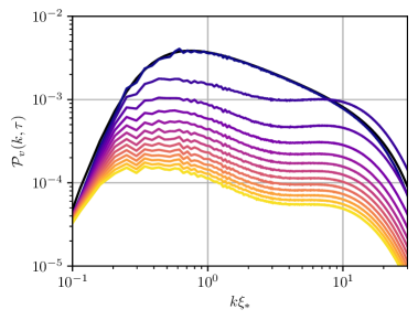
(a) Simulation (A), unrescaled velocity power spectrum.

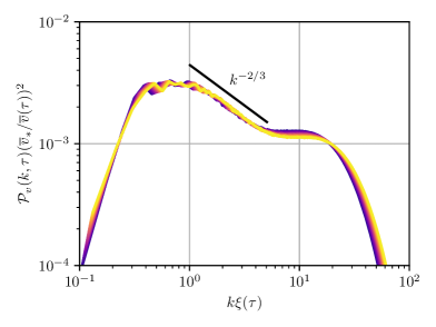
(b) Power spectrum rescaled with Eq. 3.16.

Figure 3: Evolution of the velocity power spectrum from simulation (A). Left panel: unrescaled power spectrum. The solid black line is the initial condition, Eq. 3.13 and coloured lines show the time evolution from $\tau=\tau_{*}$ up to $\tau=\tau_{\mathrm{end}}$ with interval $\Delta\tau=9.96\,\tau_{\xi_{*}}$. Lighter colours refer to later times. Right panel: power spectrum rescaled according to Eq. 3.16. The curves are plotted starting from $\tau-\tau_{*}\simeq 40\,\tau_{\xi_{*}}$, at fixed intervals $\Delta\tau=1.99\tau_{\xi_{*}}$.

Here we use the results from simulation (A) (Table 2) to investigate the time evolution of the velocity power spectrum, and the values of the parameters $\beta$, $p$ and $q$, introduced in Section 3.2.

In Fig. 3 we show the time evolution of the velocity power spectrum. Fig. 3a shows the velocity power spectrum in its raw form, whilst Fig. 3b shows the power spectrum rescaled with Eq. 3.16, indicating that there is indeed only one principal length scale in the flow, given our initial condition. The self-similarity is established starting from about $40\tau_{\xi_{*}}$, the time to which the first power spectrum line in Fig. 3b corresponds. Note that the large-scale slope of the late-time power spectrum is significantly less steep than the $k^{5}$ corresponding to the Batchelor power spectrum imposed in the initial condition Eq. 3.13: therefore, the large-scale power spectrum is not constant in time in the simulation, before about $40\tau_{\xi_{*}}$. While the large-scale slope could be subject to finite volume effects, its constancy in time seems to be well established at late times.

Turning to the form of the velocity power spectrum at wavenumbers higher than the peak, we see from Fig. 3 evidence for a power law in the range $1\lesssim k\xi_{*}\lesssim 5$. This power law is approximately consistent with a Kolmogorov power spectrum ($k^{-2/3}$) at late times. Although this was also the power spectrum in the initial conditions, one can see that this power law is lost in the early evolution, but later regained. We do not have the inertial range to give a firm value for the late-time power law index. For wavenumbers above $k\xi_{*}\gtrsim 5$, we see a small build up in power followed by a sharp fall-off for $k\xi_{*}\gtrsim 10$. The fall-off is set by the viscous damping scale of the numerical scheme, while the build up seems to be an associated feature of the van Leer advection scheme.

In Fig. 4a we plot the combination $\overline{v}^{2}\xi^{1+\beta}$, predicted to be constant when the large-scale power spectrum is constant as well, see Eq. 3.18. It can be seen that this combination indeed remains approximately constant after about $40\tau_{\xi_{*}}$, provided $\beta=3$. Consequently, in Fig. 4b we analyse again the self similarity of the power spectrum, this time rescaled according to Eq. 3.19 setting $\beta=3$. Again, we only plot the rescaled spectra for $\tau-\tau_{*}\gtrsim 40\,\tau_{\xi_{*}}$. It appears that the self-similarity condition Eq. 3.19 is satisfied by the simulation with $\beta=3$. This result is consistent with the findings of Ref. [58]. However, the large-scale power spectrum is less steep than $k^{4}$, which is the power law which would be inferred setting $\beta=3$.

Simulation (A), therefore, seems broadly consistent with the self-similar behaviour outlined in Eq. 3.19, at late times. We have seen that $\beta$ is not set by the slope of the power spectrum at low wavenumbers in the initial condition; rather, it seems to be part of the dynamics of self-similarity. We would need even larger lattices to study in detail the evolution of the power spectrum at low wavenumbers, where there appear to be correlations established at scales greater than the integral scale. Limitations of the size of the computational domain are known to possibly affect the interpretation of the turbulent decay features [66].

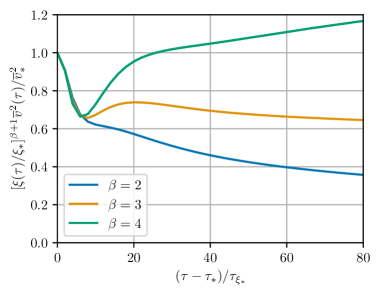
(a) Evolution of $\overline{v}^{2}\xi^{1+\beta}$.

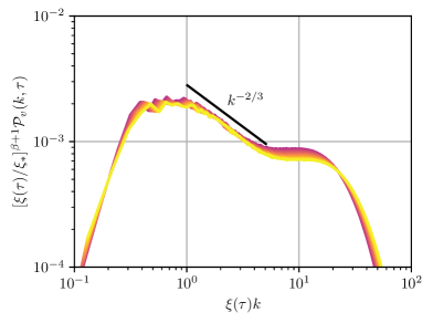
(b) Power spectrum rescaled with Eq. 3.19, assuming $\beta=3$.

Figure 4: Left panel: evolution of $\overline{v}^{2}\xi^{1+\beta}$ for different values of $\beta$ in simulation (A). As shown in Eq. 3.18, this quantity is expected to remain constant, thus indicating that $\beta\simeq 3$. Right panel: Power spectrum rescaled with Eq. 3.19, using $\beta=3$. The power spectra are plotted from $\tau-\tau_{*}\simeq 40\,\tau_{\xi_{*}}$ onward, at fixed interval $\Delta\tau=1.99\tau_{\xi_{*}}$.

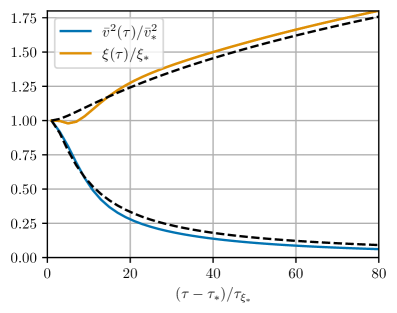
Figure 5: Evolution of the velocity and integral scale in simulation (A). The black-dashed line showcases Eqs. 3.21 and 3.22 for $\mathcal{N}_{\mathrm{e}}=5$, $p=4/3$ and $q=1/3$, where the values of $p$ and $q$ correspond to $\beta=3$; see the relationships in Eqs. 3.23 and 3.24.

In Fig. 5 we show the ratios $\overline{v}^{2}(\tau)/\overline{v}_{*}^{2}$ and $\xi(\tau)/\xi_{*}$ extracted from simulation (A), where $\overline{v}^{2}(\tau)$ and $\xi(\tau)$ are calculated by integrating the velocity power spectra of Fig. 3a, according to Eqs. 3.8 and 3.11. We also show the predicted evolution according to Eqs. 3.21 and 3.22 with $\mathcal{N}_{\mathrm{e}}=5$ (black, dashed lines), where this specific value has been chosen to match the simulation result. We fix the decay exponents in Eqs. 3.21 and 3.22 to $p=4/3$ for the kinetic energy and $q=1/3$ for the integral scale. These exponent values are provided by the condition $\beta=3$ from Eqs. 3.23 and 3.24 and provide a good fit to the simulation outcome. We shall see later in Section 7.2.2 that the precise values of the decay exponents do not have a significant effect on the final SGWB spectrum. Instead, we will see in Section 7.3 that the initial phase preceding the generation of the turbulence plays a much larger role in determining the spectral shape.

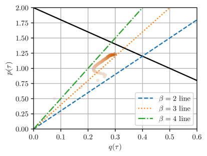
(a) Instantaneous exponents $(p,q)$.

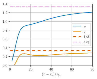
(b) Time evolution $p(\tau)$, $q(\tau)$.

Figure 6: Left panel: Trajectory of the instantaneous exponents $(p,q)$ in simulation (A). Time is represented by the colour scheme: early times are shown with lighter shades and late times with darker shades, starting at $\tau=\tau_{*}$ and with interval $\Delta\tau\simeq 2\tau_{\xi_{*}}$ between markers. The dark solid line represents the scale-invariance line $p=2(1-q)$, Eq. 3.25. The coloured dashed, dotted and dash-dotted lines show the self-similarity relations $p=(1+\beta)q$ for various choices of $\beta$. Right panel: Evolution of the instantaneous kinetic energy and integral scale exponents $(p,q)$ as a function of time in simulation (A). The dash-dotted line shows the values expected for $p$ and long dashed line for $q$, with $\beta=3$.

We further analyse the behaviour of the power law exponents $p$ and $q$ of the kinetic energy and integral scale in Fig. 6. In Fig. 6a, we adopt the same approach as Ref. [58] and plot the state of the system in $(p,q)$ space for a range of times during the simulation. The values of $p$ and $q$ are found by solving Eqs. 3.21 and 3.22 for $p$ and $q$ in terms of the measured values of $\overline{v}^{2}(\tau)$, (3.8), and $\xi(\tau)$, (3.11). The scale-invariance line $p=2(1-q)$, derived in Eq. 3.25, is represented by the black line in Fig. 6a. The self-similarity lines $p=(1+\beta)q$ are shown for various values of $\beta$ as dashed lines. As in clear from the figure, the point $(p,q)$ is still evolving at the end of the simulation. However, the evolution is moving in the direction of the intersection of the self-similarity line $p=(1+\beta)q$ with $\beta=3$, and the scale invariance line, $p=2(1-q)$. In Fig. 6b, we display the evolution of $p$ and $q$ against time, and also show the values that can be predicted from requiring scale-invariance and self-similarity for $\beta=3$, namely $p=4/3$ and $q=1/3$.

6.2 Unequal time velocity correlations

In this subsection we report on our results for the decorrelation of the velocity field at different times. We introduce a new model for the unequal time correlator and test it against the numerical simulations.

Our model for the normalized UETC is obtained by combining Eqs. 3.33, 3.36 and 4.8 giving

$$R_{\mathrm{A+}}(k,\tau,\zeta)=\frac{v_{\mathrm{dc}}(k,\tau,\zeta)}{\sqrt{v_{\mathrm{dc}}(k,\tau)v_{\mathrm{dc}}(k,\zeta)}}\exp\quantity[-\frac{1}{2}k^{2}v_{\mathrm{dc}}^{2}(k,\tau,\zeta)(\tau-\zeta)^{2}].$$ (6.1)

The factor in front of the exponential guarantees that the shear stress UETC is a positive definite kernel and hence that the resulting gravitational wave power spectrum is positive definite, as explained in Section 4.1. This is to be compared with the model of Ref. [38],

$$R_{\mathrm{NSS}}(k,\tau,\zeta)=\exp\quantity[-\frac{1}{2}k^{2}v_{\mathrm{dc}}^{2}(k,\zeta)(\tau-\zeta)^{2}],\quad\tau>\zeta\,.$$ (6.2)

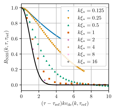
(a) Model of Ref. [39].

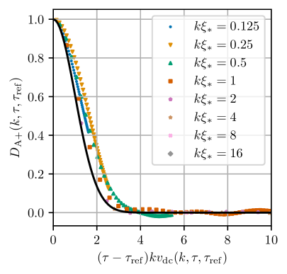
(b) Our model.

Figure 7: Comparison of normalized unequal time correlator models with data from simulation (A): on the left, the model of Ref. [39] as used in Ref. [38], on the right our model. The $y$-axis displays the combination of data and model functions which should produce a Gaussian curve in the argument of the $x$-axis; this is discussed in further detail in connection with Eq. 6.3. The solid dark line is the prediction of the model in each case.

In Fig. 7, we compare the two models to data from simulation (A), by plotting combinations of data and model functions which should be of Gaussian form. Results from the other simulations are given in Appendix D. The construction of the numerical UETC, $P_{v}(k,\tau,\zeta)$ is described in Section 5.4; in our simulations we measure the correlation of the velocity field at times $\zeta=\tau_{\mathrm{ref}}$ and $\tau$.

For our model, the data is plotted as the quantity

$$D_{\mathrm{A}+}(k,\tau,\tau_{\mathrm{ref}})\equiv\frac{P_{v}(k,\tau,\tau_{\mathrm{ref}})}{\sqrt{P_{v}(k,\tau)\,P_{v}(k,\tau_{\mathrm{ref}})}}\sqrt{\frac{v_{\mathrm{dc}}^{2}(k,\tau)+v_{\mathrm{dc}}^{2}(k,\tau_{\mathrm{ref}})}{2v_{\mathrm{dc}}(k,\tau)v_{\mathrm{dc}}(k,\tau_{\mathrm{ref}})}},$$ (6.3)

against the combination $k\,v_{\mathrm{dc}}(k,\tau,\tau_{\mathrm{ref}})(\tau-\tau_{\mathrm{ref}})$, while for the model of Ref. [38], we plot the normalized velocity UETC (3.26) as a function of $k\,v_{\mathrm{dc}}(k,\tau_{\mathrm{ref}})(\tau-\tau_{\mathrm{ref}})$. We choose a range of values for the wavenumber $k$, both larger and smaller than the inverse integral scale $\xi_{*}$. The reference time is taken to be approximately one initial eddy turnover time, $\tau_{\mathrm{ref}}\simeq\tau_{\xi_{*}}=\xi_{*}/\overline{v}_{*}$ (see Table 2). The success of the models can be judged by how well all the data from simulations collapses onto a Gaussian in the $x$-axis argument, indicated by the black lines.

From Fig. 7 it appears that both models work well in the inertial range $k\xi_{*}\gg 1$. This demonstrates that the sweeping model, with sweeping velocity $\overline{v}/\sqrt{3}$, characterizes very well the decorrelation of the system at high wavenumbers, and that we may take $C_{v}^{2}=1$ in Eq. 3.35. This also indicates that models using the scale-dependent Lagrangian eddy turn-over time $v^{2}_{\mathrm{dc}}(k,\tau_{\mathrm{ref}})\propto\mathcal{P}_{v}(k,\tau_{\mathrm{ref}})$ in the inertial range [6, 33] give a poor fit in the inertial range.

On the other hand, the decorrelation model based on Eq. 6.2 degrades somewhat for $0.125\leq k\xi_{*}\leq 1$. Our decorrelation model is a significant improvement on these scales, which we ascribe partly to the fact that the average decorrelation velocity takes into account the slowing of the decorrelation with the decay of the kinetic energy.

Because of limitations in the dynamical range of the simulations, it is not possible to analyse very small values of $k\xi_{*}$. However, we will see that the GW power spectrum decreases at small $k\xi_{*}$, and so it is less important to model accurately the UETC at wavenumbers well below the peak.

Note that according to recent work in Ref. [71], the Gaussian form of the random sweeping hypothesis should change to an exponential form at large time differences. Again, this effect should be most influential at low $k$, below the peak of the power spectrum. We leave further study of UETC models for future work.

7 Results: the gravitational wave spectrum

This section is organized as follows. In Section 7.1 we study a stationary source, meaning that we assume that $P_{v}(p,\tau,\zeta)$ only depends on the time difference $\tau-\zeta$. This is not the correct model for freely decaying turbulence, but we consider it nonetheless since it is useful to illustrate some properties of the GW power spectrum of a freely decaying source.

We present the case of freely decaying turbulence in the subsequent Sections 7.2 and 7.3. Section 7.2 contains the main results of our work, and is dedicated to the case of instantaneously generated turbulence, meaning that we insert as initial conditions a fully developed turbulent spectrum. Finally, in Section 7.3, we go beyond the instantaneous generation scenario, and include a growth phase for the turbulence kinetic energy.

Before continuing, we first set the basis for the calculation of the stochastic GW background that will follow. Combining Eqs. 2.15 and 2.24, one obtains (recall that $\mathbf{q}=\mathbf{k}-\mathbf{p}$)

$$\evaluated{\derivative{{\Omega}_{\mathrm{gw}}}{\ln k}}_{\tau}=\frac{k^{3}}{3\pi^{5}}\int\differential[3]{p}\quantity[1+(\hat{\mathbf{k}}\dotproduct\hat{\mathbf{p}})^{2}]\quantity[1+(\hat{\mathbf{k}}\dotproduct\hat{\mathbf{q}})^{2}]\iint_{\tau_{\mathrm{ini}}}^{\tau}\mathcal{G}(k,\tau,\eta,\zeta)P_{v}(p,\eta,\zeta)P_{v}(q,\eta,\zeta)\frac{\differential{\eta}}{\eta}\frac{\differential{\zeta}}{\zeta}.$$ (7.1)

From this expression, it appears that the computation of the GW background involves performing a five-dimensional integration for each mode $k$. Integrating over the azimuthal angle of $\mathbf{p}$ immediately gives a factor of $2\pi$ and one is left with a four-dimensional integration. Technical details on how to tackle this four-dimensional integration are presented in Appendix A. In particular, we advocate the change of variables $\mathbf{p}=\mathbf{k}/2+\mathbf{h}$ (and hence $\mathbf{q}=\mathbf{k}/2-\mathbf{h}$): this makes the symmetry around the zero of the cosine of the declination angle $\alpha=\hat{h}\cdot\hat{k}$ explicit.

After the complete decay of turbulence, occurring at a time that we denote $\tau_{\mathrm{fin}}$, the GW power spectrum in the radiation era evolves as

$$\evaluated{\derivative{\Omega_{\mathrm{gw}}}{\ln k}}_{\tau\geq\tau_{\mathrm{fin}}}=\frac{8}{3\pi^{2}}k^{3}\iint_{\tau_{\mathrm{ini}}}^{\tau_{\mathrm{fin}}}\mathcal{G}(k,\tau,\eta,\zeta)P_{\tilde{\Pi}}(k,\eta,\zeta)\frac{\differential{\eta}}{\eta}\frac{\differential{\zeta}}{\zeta}.$$ (7.2)

This can be obtained by matching the sourced and free solutions of Eq. 2.2 at time $\tau_{\mathrm{fin}}$. Note that the function $\mathcal{G}$ of Eq. 2.14 depends explicitly on $\tau$, meaning that the GW spectrum in principle still depends on time after the source has decayed. We are interested in the GW spectrum at a time $\tau$ in the radiation era long after the source has decayed, and such that all relevant wavenumbers are inside the horizon, $k\tau>1$. This way we can neglect the second and third terms in Eq. 2.14, proportional to $1/(k\tau)$ and $1/(k\tau)^{2}$, since they become subdominant with respect to the first one. Furthermore, we can expand the first term of Eq. 2.14 to obtain

$$\evaluated{\derivative{\Omega_{\mathrm{gw}}}{\ln k}}_{\tau\geq\tau_{\mathrm{fin}}}=\, \frac{4}{3\pi^{2}}k^{3}\iint_{\tau_{\mathrm{ini}}}^{\tau_{\mathrm{fin}}}\cos k(\eta-\zeta)P_{\tilde{\Pi}}(k,\eta,\zeta)\frac{\differential{\eta}}{\eta}\frac{\differential{\zeta}}{\zeta}$$

$$+\frac{4}{3\pi^{2}}k^{3}\cos(2k\tau)\iint_{\tau_{\mathrm{ini}}}^{\tau_{\mathrm{fin}}}\sin k(\zeta+\eta)P_{\tilde{\Pi}}(k,\eta,\zeta)\frac{\differential{\eta}}{\eta}\frac{\differential{\zeta}}{\zeta}$$

$$+\frac{4}{3\pi^{2}}k^{3}\sin(2k\tau)\iint_{\tau_{\mathrm{ini}}}^{\tau_{\mathrm{fin}}}\cos k(\zeta+\eta)P_{\tilde{\Pi}}(k,\eta,\zeta)\frac{\differential{\eta}}{\eta}\frac{\differential{\zeta}}{\zeta}+\order{(k\tau)^{-1}}$$ (7.3)

The residual time dependence consists of irrelevant, rapid oscillations in time. We can therefore perform a time average of the free SGWB solution over a long time interval around $\tau$, satisfying $\Delta\tau\gg 1/k$ for every interesting $k$, to obtain

$$\derivative{\Omega_{\mathrm{gw}}}{\ln k}\approx\frac{4}{3\pi^{2}}k^{3}\iint_{\tau_{\mathrm{ini}}}^{\tau_{\mathrm{fin}}}\cos k(\eta-\zeta)P_{\tilde{\Pi}}(k,\eta,\zeta)\frac{\differential{\eta}}{\eta}\frac{\differential{\zeta}}{\zeta}\,.$$ (7.4)

This is the effectively time-independent GW power spectrum that we aim to calculate. Recall that $\Omega_{\mathrm{gw}}$ is normalized to the radiation energy density, see Eq. 2.15. Therefore, long after the source has decayed, the averaged energy density of the GW signal would be expected to decrease as $a(\tau)^{-4}$.

7.1 The stationary assumption

In this section, we simplify the evaluation of the GW spectrum integral of Eq. 7.4 by assuming that the turbulence is stationary. Under this assumption, the rms velocity $\overline{v}$ and the integral scale $\xi$ remain constant in time. We further set the decorrelation velocity to $v_{\mathrm{dc}}\equiv\overline{v}_{*}/\sqrt{3}$ on all scales. In other words, we neglect the $k$-dependence in Eq. 3.38. Motivated by what we see in the simulations, we also set $C_{v}^{2}=1$ in Eq. 3.35. Consequently, the only time dependence left in the UETC in Eq. 4.7 is the time difference in the exponential. In order to evaluate Eq. 7.4 under the hypothesis that the source is stationary, it therefore becomes natural to change the time integration variables to $\tau_{\mathrm{mid}}=(\tau+\zeta)/2$ and $\tau_{\mathrm{diff}}=\tau-\zeta$, where the integration over the latter is symmetric around zero. We give the form that Eq. 7.4 takes under this stationary assumption as Eq. B.1.

In order to proceed analytically, we rely on the exponential decorrelation, and extend the integration limits of $\tau_{\mathrm{diff}}$ to the interval $[0,\infty[$. Furthermore, one can also assume that the time difference $\tau_{\mathrm{diff}}$ is small compared to the absolute time $\tau_{\mathrm{mid}}$. Under these two further assumptions, which are not strictly speaking a direct consequence of stationarity, one can integrate Eq. B.1 analytically.

A stationary source in principle lasts forever. However, this is not very realistic in the early Universe setting. We will therefore fix the source duration to a finite value that we express in terms of $\mathcal{N}_{\mathrm{cut}}$, the number of eddy turnover times for which the turbulence lasts. In other words, we integrate from $\tau_{*}$ until $\tau_{*}+\mathcal{N}_{\mathrm{cut}}\tau_{\xi_{*}}$. The result then depends explicitly on $\mathcal{N}_{\mathrm{cut}}$.

In Appendix B we provide the details of the integration procedure. The asymptotic behaviour of the resulting SGWB spectrum, and its scaling with the turbulence parameters are given by

$${\derivative{{\Omega}_{\mathrm{gw}}}{\ln k}}\quantity(K\ll 1) =c_{1}\,\frac{\mathcal{N}_{\mathrm{cut}}\,(\mathcal{H}_{*}\xi_{*})^{2}}{\overline{v}_{*}+\mathcal{N}_{\mathrm{cut}}\mathcal{H}_{*}\xi_{*}}\,\overline{v}_{*}^{6}\,\quantity(\frac{K}{\overline{v}_{*}})^{3};$$ (7.5)

$${\derivative{{\Omega}_{\mathrm{gw}}}{\ln k}}\quantity(K\gg 1) =\frac{\mathcal{N}_{\mathrm{cut}}\,(\mathcal{H}_{*}\xi_{*})^{2}}{\overline{v}_{*}+\mathcal{N}_{\mathrm{cut}}\mathcal{H}_{*}\xi_{*}}\,\quantity[c_{2}\,\overline{v}_{*}^{6}\,\quantity(\frac{K}{\overline{v}_{*}})^{-\frac{7}{3}}+c_{3}\,\overline{v}_{*}^{4/3}\,\exp(-\frac{3}{2\overline{v}_{*}^{2}})\quantity(\frac{K}{\overline{v}_{*}})^{-\frac{5}{3}}]$$ (7.6)

(note that $K=\mathcal{A}\xi k$, and the value of the numerical coefficients $c_{i}$ are given in Appendix B).

Eqs. 7.5 and 7.6 show that the scaling of the GW signal with the parameter $\mathcal{H}_{*}\xi_{*}$ depends on the source duration. If the sourcing lasts less than one Hubble time, meaning $\mathcal{N}_{\mathrm{cut}}\tau_{\xi_{*}}=\mathcal{N}_{\mathrm{cut}}\xi_{*}/\overline{v}_{*}<\mathcal{H}_{*}^{-1}$, one can neglect the second term in the denominator of Eqs. 7.5 and 7.6, and the SGWB scaling becomes quadratic in $\mathcal{H}_{*}\xi_{*}$. On the other hand, if the source lasts longer than one Hubble time, the scaling is linear in $\mathcal{H}_{*}\xi_{*}$ (see for example Refs. [24, 25, 36, 32, 8]). If we had set the duration of the source to infinity, as required in principle by the stationary assumption, we would have consistently found a linear dependence on $\mathcal{H}_{*}\xi_{*}$.

Gravitational wave generation from sound waves also presents the same duration-dependent scaling with $\mathcal{H}_{*}\xi_{*}$. This was previously derived within the sound shell model [24, 27, 86, 87]. In the sound shell model one can also assume stationarity and set $\mathcal{N}_{\mathrm{cut}}\sim 1$ as in Ref. [87]. Note that, in the acoustic case, the decorrelation time depends on the sound speed, instead of on the rms fluid velocity. The typical lifetime of the source is connected to the kinetic energy. For the turbulent case, low velocities correspond to longer eddy turnover times $\tau_{\xi_{*}}=\xi_{*}/\overline{v}_{*}$, and therefore sources that last longer. The kinetic energy is in turn expected to be connected to the PT strength (see for example Ref. [88]). The latter then ultimately influences the scaling of the SGWB amplitude [8].

The turbulent kinetic energy also naturally enters the SGWB amplitude, through $\overline{v}_{*}$. In particular, the stationary assumption leads to a stronger scaling with $\overline{v}_{*}$ than both the case of instantaneous generation (see Section 7.2) and the SGWB signal arising from sound waves [27, 86]: at large scales and/or for low initial turbulent velocity, Eqs. 7.5 and 7.6 show that the SGWB amplitude from turbulence within the stationary assumption scales as $\overline{v}_{*}^{6}$, as opposed to $\overline{v}_{*}^{4}$ for both sound waves and an instantaneous turbulence generation (as we shall see in Section 7.2).

We remark that the value of $\overline{v}_{*}$ also influences the high-frequency slope of the SGWB, see Eq. 7.6. This is a consequence of the exponential decorrelation in the velocity power spectrum Eq. 4.7. For large $\overline{v}_{*}>0.5$, the second term in Eq. 7.6 dominates: consequently, the SGWB spectrum becomes shallower, and its amplitude scales as $\overline{v}_{*}^{4/3}$. The slope of the SGWB at low wavenumber, on the other hand, is due to the steep (causal) increase of the velocity power spectrum Eq. 3.13, causing the convolution in Eq. 2.24 to be flat for $k<1/\xi_{*}$ (uncorrelated in space for scales larger than $\xi_{*}$) [32]. The complete spectral shape can be obtained by integrating numerically Eq. B.4: it smoothly interpolates between the slopes given by Eqs. 7.5 and 7.6, peaking at the wavenumber $k\simeq 2\overline{v}_{*}/(\mathcal{A}\xi_{*})$. Examples of spectra are given in Appendix B.

7.2 Instantaneous turbulence generation

In this section, we consider turbulence generated instantaneously, and freely decaying afterwards. We consider a situation where gravitational wave production begins when the fluid has the velocity spectrum of fully developed turbulence, at time $\tau_{*}$. We use three different methods to compute the SGWB spectrum. First, we measure the SGWB in the simulations. Second, we numerically integrate Eq. 7.4 inserting the model for freely-decaying turbulence derived in the first part of this paper, summarized in Eq. 4.7 (see also section Section 6). Third, we assume that the GW source is constant in time, and analytically integrate Eq. 7.3 under this assumption. We show that there is good agreement between the three methods for the resulting SGWB. In particular, the analytical approximation provides an easy-to-use formula, Eq. 7.16, in which the scaling with the turbulence parameters (initial rms velocity, integral scale, duration) is apparent.

7.2.1 Simulations

In Fig. 8 we present GW power spectra from three simulations with $\overline{v}_{*}\approx 0.1$, corresponding to simulations (A), (D) and (E) in Table 2. Equivalent plots for the other simulations are given in Appendix E. We explore different regions of the power spectrum with each simulation. Simulation (D) has a large value of $L\differential{x}/\xi_{*}$ and is therefore able to probe the GW power spectrum around the peak and towards smaller $k$, whereas simulation (E) is better able to probe the inertial range due to the smaller value of $\differential x/\xi_{*}$. Simulation (A) has more lattice sites, allowing for a larger dynamic range. For this simulation we chose $L\differential{x}/\xi_{*}$ and $\differential x/\xi_{*}$ such that they lie in between the values of simulations (D) and (E). Simulation (A) then probes the peak of the spectrum and intermediate wavenumbers, confirming the power laws at low and high wavenumbers in these regions.

The SGWB power spectrum builds up very rapidly - this is further discussed in Section 7.2.3; its shape reflects the initial power spectrum, $\mathcal{P}_{U}$ of Eq. 5.6, representing fully developed turbulence.

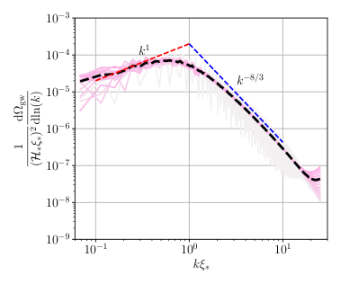
(a) Simulation (A), $\Delta\tau/\tau_{\xi_{*}}=3.98$.

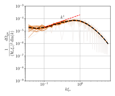
(b) Simulation (D), $\Delta\tau/\tau_{\xi_{*}}=4.87$.

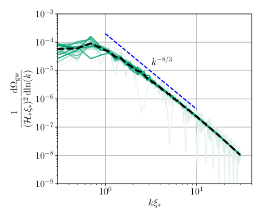
(c) Simulation (E), $\Delta\tau/\tau_{\xi_{*}}=0.594$.

Figure 8: Gravitational wave power spectrum from our simulations with $\overline{v}_{*}\approx 0.1$. In the y-axis, we divide the by $(\mathcal{H}_{*}\xi_{*})^{2}$ since the simulations are in flat space-time, see Eq. 5.18 and the following discussion. The coloured lines show the gravitational wave power spectrum at intervals $\Delta\tau$ starting from $\tau-\tau_{*}=\Delta\tau$ and finishing at $\tau=\tau_{\mathrm{end}}$ . Darker shades correspond to later times. The black dashed line shows an average over the gravitational wave power spectrum in the last half of the elapsed simulation time. The red dashed line shows a $k^{1}$ power-law, while the blue dashed line shows a $k^{-8/3}$. The sampling of relatively few $k$-space modes into discrete bins leads to some noise in the very lowest wavenumbers. It is also possible that, for these lowest wavenumbers, finite volume effects lead to a flattening of the power spectrum as this is not seen in our results using numerical integration. We have cut off the spectrum at high wavenumbers as it progressively gets polluted due to numerical precision errors in projecting $\dot{u}_{ij}(\mathbf{k})$ to $\dot{h}_{ij}(\mathbf{k})$.

By averaging over the gravitational wave power spectrum in the latter half of each simulation, we are able to smooth out time-dependent oscillations in the GW power spectrum. This averaged power spectrum is shown by the black dashed line in Fig. 8. A clear $k^{-8/3}$ power law is found for the inertial range in simulations (A) and (E), and an approximate $k^{1}$ power law at small wavenumbers is seen in (A) and (D). Taking a time average over the second half of the simulation is justified since the simulation wavenumbers satisfy $k>2/(\tau_{\mathrm{end}}-\tau_{*})$ for all simulations. This can be verified by comparing the k-range in Fig. 8 (figures for the other simulations are in Appendix E) with the values given in Table 2 (see also Table 1).

When we compute the power spectrum from our simulations, we bin modes which have a wavenumber within a given shell of $k$, as given by Eq. 5.16. At late times, the frequency of the oscillations of each mode increases and the modes in each bin begin to oscillate out of phase. Consequently, our simulations average over these oscillations and do not capture them, even when we do not perform an average over time. This process can clearly be seen for high wavenumbers in Fig. 8.

To show the variation of the GW power spectrum for different $\overline{v}_{*}$ and for different choices of $\xi_{*}/\differential x$, we plot the averaged GW power spectrum from all simulations in Fig. 9. As can be seen, simulations with different choices of $\xi_{*}/\differential x$ explore different parts of the spectrum, with small $\xi_{*}/\differential x$ mapping out low wavenumbers and the peak of the spectrum, and larger $\xi_{*}/\differential x$ exploring the inertial range. Indeed, for $\overline{v}_{*}\simeq 0.1$ we find good agreement between simulations (A) and (D) from low wavenumbers up to the vicinity of the peak, and with (E) at high wavenumbers. This gives us confidence that the results obtained for other $\overline{v}_{*}$ are also valid.

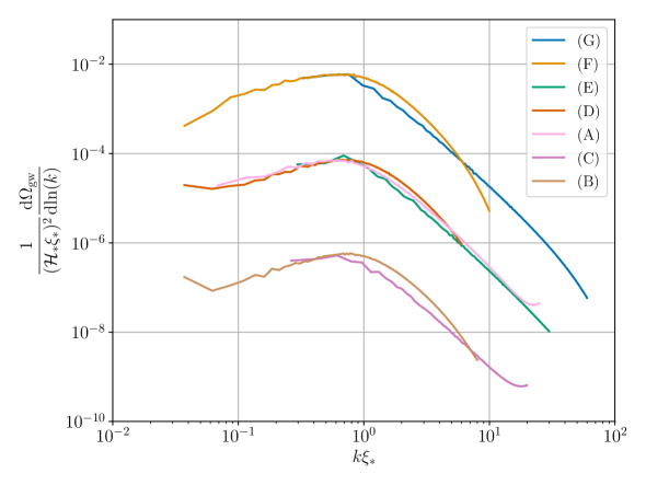
Figure 9: Averaged GW power spectra for simulations (A)-(G) from Table 2. The coloured lines shown here correspond to averaging the GW power spectra over the last half of the simulations. Simulations (B) and (C) have $\overline{v}_{*}\simeq 0.03$, (A), (D) and (E) have $\overline{v}_{*}\simeq 0.1$, and (F) and (G) have $\overline{v}_{*}\simeq 0.3$. A cut off has been applied to the spectrum at high wavenumbers due to numerical precision noise.

In subsequent sections we will show how these simulations can be compared with the results of the four dimensional numerical integration, and with the analytical result obtained under the assumption of a constant source in time. We plot all three approaches in Fig. 13 and find good agreement.

7.2.2 Gravitational wave spectrum via numerical integration of the anisotropic stress UETC

We have developed a numerical method allowing exact integration of the time-averaged SGWB spectrum, Eq. 7.4. This includes integration of the full angular dependence as well, improving on previous attempts [36, 38]. We insert Eq. 4.7 into Eq. 2.24, and in turn into Eq. 7.4. Making use of Eq. 3.9, the initial spectral density $P_{v}(k,\tau_{\mathrm{ini}})$ is set to the von Kármán spectrum Eq. 3.13, representing fully developed incompressible turbulence.

We also need to insert the time evolution laws for $\overline{v}^{2}(\tau)$ and $\xi(\tau)$. In accordance with the initial conditions adopted in the simulations (see Section 5.2), we assume instantaneous generation of turbulence. Specifically, prior to $\tau_{*}$ the velocity field is zero everywhere, then at time $\tau_{*}$, turbulence appears fully developed with initial rms velocity $\overline{v}_{*}$ and initial correlation scale $\xi_{*}$. Turbulence then starts decaying on a timescale of order $\tau_{\xi_{*}}$, following Eqs. 3.21 and 3.22. To summarize, for the instantaneous generation scenario:

$$\overline{v}^{2}(\tau)=\begin{cases}0&\text{if }\tau<\tau_{*}\\ \overline{v}_{*}^{2}\quantity(\dfrac{\tau-\tau_{*}+\mathcal{N}_{\mathrm{e}}\tau_{\xi_{*}}}{\mathcal{N}_{\mathrm{e}}\tau_{\xi_{*}}})^{-p}&\text{if }\tau>\tau_{*}\end{cases}\quad\text{and}\quad\xi(\tau)=\begin{cases}\text{Not defined}&\text{if }\tau<\tau_{*}\\ \xi_{*}\quantity(\dfrac{\tau-\tau_{*}+\mathcal{N}_{\mathrm{e}}\tau_{\xi_{*}}}{\mathcal{N}_{\mathrm{e}}\tau_{\xi_{*}}})^{q}&\text{if }\tau>\tau_{*}\end{cases}.$$ (7.7)

In the following we set $\mathcal{N}_{\mathrm{e}}=5$, the value that best fits the simulations, see Fig. 5. For the decay exponents $p,~{}q$, we tested both sets of values that one infers from Eqs. 3.23 and 3.24, setting $\beta=3$ and $\beta=4$. The unequal time decorrelation velocity appearing in the exponential of Eq. 4.7 is expressed in terms of the equal time one as in Eq. 4.8, with $v_{\mathrm{dc}}(k,\tau)$ given in Eq. 3.36. The four-dimensional integral of Eq. 7.4 is calculated with Monte Carlo integration with importance sampling, using the VEGAS algorithm [89, 90], an iterative and adaptive Monte Carlo scheme. More details on the implementation are given in Appendix A.

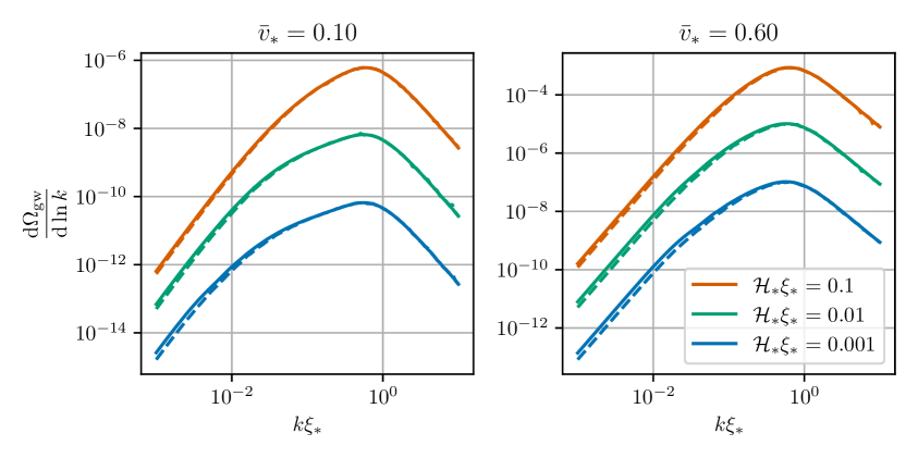
Figure 10: Examples of GW power spectra computed via numerical integration of Eq. 7.4 under the assumption of instantaneous turbulence generation (see (7.7)). The spectra are computed using different values of the initial rms velocity, $\overline{v}_{*}$, the initial integral scale relative to the Hubble scale, $\mathcal{H}_{*}\xi_{*}$. Each panel corresponds to a different value of $\overline{v}_{*}$, as specified by the title, and each colour indicates a different value of $\mathcal{H}_{*}\xi_{*}$, as specified by the legend in the bottom right panel. The solid lines are computed setting $\beta=3$, whereas the dashed lines setting $\beta=4$. We recall that the evolution of $\overline{v}(\tau)$ and $\xi(\tau)$ are determined by $\beta$ through Eqs. 3.23 and 3.24.

As discussed at the end of Section 3.2, turbulence is fully dissipated after about $1000\tau_{\xi_{*}}$ (the inertial range has disappeared), for reasonable choices of the initial parameters $T_{*},~{}\overline{v}_{*},~{}\xi_{*}\mathcal{H}_{*}$. However, there is no need to time-integrate Eq. 7.4 for so long: the bulk of the GW power spectrum is sourced on a much shorter timescale. This is due to two reasons. First, the generation of GWs is very localized in time: GWs with wavenumber $k$ are produced by the source on a timescale $\order{1/k}$, since the Green’s function in Eq. 7.1, given in Eq. 2.14, has period $2\pi/k$. Second, the decay of turbulence occurs over a timescale of the order of the initial eddy turnover time $\tau_{\xi_{*}}$, which effectively cuts off the source (more precisely, about five $\tau_{\xi_{*}}$, since $\mathcal{N}_{\mathrm{e}}\simeq 5$ is the value that best fits the simulations - see Section 3.2). All GW wavenumbers with $k\gtrsim 1/(\mathcal{N}_{\mathrm{e}}\tau_{\xi_{*}})$ are therefore sourced before the turbulent kinetic energy has decayed appreciably. This includes the peak region of the SGWB spectrum. On the other hand, GW wavenumbers with $k\lesssim 1/(\mathcal{N}_{\mathrm{e}}\tau_{\xi_{*}})$ are excited when the decay of the turbulent kinetic energy has already occurred: GW production on these wavenumbers is therefore negligible. This is the large scale spectral region, proportional to $k^{3}$. We therefore expect the GW power spectrum to stop growing after a timescale of the order of $1/(\mathcal{N}_{\mathrm{e}}\tau_{\xi_{*}})$. We have numerically checked that the integration in Eq. 7.1 indeed converges to a fixed result after a few tens of $\tau_{\xi_{*}}$.

In the code, we actually integrate for $100~{}\tau_{\xi_{*}}$: therefore, in practice we output the SGWB spectra long after the source has decayed, when the spectral amplitude does not grow in time any longer (the integral in Eq. 7.4 has converged). Furthermore, the $k$-range of interest is such that $k>1/(100\,\tau_{\xi_{*}})$ for every chosen value of $\overline{v}_{*}$ and $\mathcal{H}_{*}\xi_{*}$, as can be appreciated from Fig. 10. Therefore, we are allowed to integrate directly the time-averaged GW spectrum Eq. 7.4. We have indeed checked that numerically integrating the full expression Eq. 7.3 provides a GW spectrum which is oscillating around the amplitude of the integral of the time-averaged GW spectrum, Eq. 7.4, shown in Fig. 10. We do not plot these spectra, as they do not convey any additional information.

Fig. 10 shows the GW power spectrum computed from the numerical integration code, for different values of the parameters $\overline{v}_{*}$ and $\mathcal{H}_{*}\xi_{*}$ and for both $\beta=3$ and $\beta=4$. It can be appreciated that the peak amplitude scales like $(\mathcal{H}_{*}\xi_{*})^{2}$. The spectral peak is independent of the value of $\overline{v}_{*}$, and corresponds to the peak of the velocity power spectrum Eq. 3.13, occurring at $k\xi_{*}\simeq 2.7/\mathcal{A}$. This is consistent with the finding of Ref. [77] for a source which is discontinuous in time.

The spectra which have $\mathcal{H}_{*}\xi_{*}=10^{-3}$ in Fig. 10 are minimally affected by the expansion of the Universe: the chosen values of $\overline{v}_{*}$ and $\mathcal{H}_{*}\xi_{*}$ satisfy $100\,\tau_{\xi_{*}}\leq\mathcal{H}_{*}^{-1}$, and so the dynamics take place fully at sub-horizon scales. It is therefore appropriate to compare these spectra to the time-averaged spectra resulting from the simulations, in the region $k>\mathcal{H}_{*}$ (see Eq. 5.18 and discussion thereafter). We will do so in sub-Section 7.2.4. On the other hand, for larger values of $\mathcal{H}_{*}\xi_{*}$ in Fig. 10, we integrate for longer than one Hubble time.

We find that the actual values of the exponents $p$ and $q$ do not substantially impact the SGWB spectrum, indicating that the precise details of the turbulent decay are unimportant in this respect. This is due to the nature of the free decay of turbulence in combination with the typically short timescale associated with GW production. Fig. 10 shows the SGWB spectrum from the numerical integration for both $\beta=3$ and $\beta=4$. For all values of $\overline{v}_{*}$ and $\mathcal{H}_{*}\xi_{*}$ the spectra only differ in the region $k<1/(\mathcal{N}_{\mathrm{e}}\tau_{\xi_{*}})$, as expected for reasons we have outlined above. For the same reasons, we can safely ignore the role of the viscous scale $\lambda$ in all our evaluations.

7.2.3 Constant source approximation

In this section, we show that the GW source can be approximated as almost constant in time while the majority of the GW signal is being generated. This has already been pointed out in Ref. [46], in the case of MHD turbulence. Since the Green’s function in Eq. 7.1 has period $2\pi/k$, the GW production for each wavenumber $k$ occurs on a timescale of the order of $1/k$. Therefore, over the typical decay time for the turbulence source, namely $\mathcal{N}_{\mathrm{e}}\tau_{\xi_{*}}$ – as we assumed for Eq. 7.7 – there is sourcing of gravitational waves for wavenumbers $k>1/(\mathcal{N}_{\mathrm{e}}\tau_{\xi_{*}})\equiv\overline{v}_{*}/(\mathcal{N}_{\mathrm{e}}\xi_{*})$. This constitutes a large fraction of the GW spectrum, including the region around the peak $k\,\xi_{*}\simeq 2.7/\mathcal{A}$. Consequently, the SGWB signal on the scales of interest – specifically, around the peak – is fully established before the turbulence has decayed appreciably. On scales larger than the peak, on the other hand, the GW production is less efficient due to the decay of the source. On even larger scales, one expects the $k^{3}$ increase typical of uncorrelated sources in both time and space [77].

We assume in what follows that the turbulent GW source is instantaneously generated, remains constant for a duration $\mathcal{N}_{\mathrm{cut}}\tau_{\xi_{*}}$, and sharply turns off at a time $\tau_{*}+\mathcal{N}_{\mathrm{cut}}\tau_{\xi_{*}}$. The number $\mathcal{N}_{\mathrm{cut}}$ is of the same order as $\mathcal{N}_{\mathrm{e}}$, and we set $\mathcal{N}_{\mathrm{cut}}$ to $7$ as it gives the best fit to the result of the numerical integration. We neglect both the overall time dependence of the turbulent fluid velocity power spectrum and its time decorrelation in Eq. 4.7 This means that the anisotropic stress spectral density Eq. 2.24 becomes time-independent, and the time and momentum integrals in Eq. 7.1 decouple. We can then rewrite Eq. 7.2 as

$$\evaluated{\derivative{{\Omega}_{\mathrm{gw}}}{\ln k}}_{\tau_{*}+\mathcal{N}_{\mathrm{cut}}\tau_{\xi_{*}}}=\frac{8}{3\pi^{2}}\,k^{3}\,\mathcal{T}_{\mathrm{gw}}(k,\tau_{*},\mathcal{N}_{\mathrm{cut}}\tau_{\xi_{*}})\,P_{\tilde{\Pi}}(k,\tau_{*})\,.$$ (7.8)

Let us first analyse the part due to the double time integral $\mathcal{T}_{\mathrm{gw}}$. We evaluate it at the source turn-off:

$$\mathcal{T}_{\mathrm{gw}}(k,\tau_{*},\mathcal{N}_{\mathrm{cut}}\tau_{\xi_{*}})\equiv\iint_{\tau_{*}}^{\tau_{*}+\mathcal{N}_{\mathrm{cut}}\tau_{\xi_{*}}}\mathcal{G}(k,\tau_{*}+\mathcal{N}_{\mathrm{cut}}\tau_{\xi_{*}},\eta,\zeta)\,\frac{\differential{\eta}}{\eta}\frac{\differential{\zeta}}{\zeta}.$$ (7.9)

Restricting our consideration of this integral to wavenumbers satisfying $k>1/(\tau_{*}+\mathcal{N}_{\mathrm{cut}}\tau_{\xi_{*}})$, we are again entitled to drop the second and third term from the Green’s function Eq. 2.14, to obtain [46]:

$$\mathcal{T}_{\mathrm{gw}}(k,\tau_{*},\mathcal{N}_{\mathrm{cut}}\tau_{\xi_{*}}) =\iint_{\tau_{*}}^{\tau_{*}+\mathcal{N}_{\mathrm{cut}}\tau_{\xi_{*}}}\cos k(\tau_{*}+\mathcal{N}_{\mathrm{cut}}\tau_{\xi_{*}}-\eta)\cos k(\tau_{*}+\mathcal{N}_{\mathrm{cut}}\tau_{\xi_{*}}-\zeta)\frac{\differential{\eta}}{\eta}\frac{\differential{\zeta}}{\zeta}$$ (7.10)

$$=\left\{\cos k(\tau_{*}+\mathcal{N}_{\mathrm{cut}}\tau_{\xi_{*}})\quantity[\operatorname{Ci}(k(\tau_{*}+\mathcal{N}_{\mathrm{cut}}\tau_{\xi_{*}}))-\operatorname{Ci}(k\tau_{*})]\right.$$

$$\qquad+\left.\sin k(\tau_{*}+\mathcal{N}_{\mathrm{cut}}\tau_{\xi_{*}})\quantity[\operatorname{Si}(k(\tau_{*}+\mathcal{N}_{\mathrm{cut}}\tau_{\xi_{*}}))-\operatorname{Si}(k\tau_{*})]\right\}^{2}.$$ (7.11)

The upper limits of both time integrals must be set to $\tau_{\mathrm{fin}}=\tau_{*}+\mathcal{N}_{\mathrm{cut}}\tau_{\xi_{*}}$ in order to match the results of both the simulations and the numerical integration (see Section 7.2.4). As pointed out in Ref. [46], the abrupt switching off of the source means that the evolution after $\tau_{\mathrm{fin}}$ would give an enhancement of the SGWB power at high frequency, which would break this agreement. Since we evaluate the time integrals at $\tau_{\mathrm{fin}}$, we cannot perform a time average; this is why we do not use Eq. 7.4 in this Section.

In Ref. [46], a simplified expression for Eq. 7.10 has been found, tuned to interpolate the envelope of the $k$-oscillations. In this work, we want to compare with the results of the simulations (Section 7.2.1) and of the numerical integration (Section 7.2.2), which both evaluate the time-averaged SGWB. We therefore adapt the result of Ref. [46] to account for time averaging, as follows:

$$\mathcal{T}_{\mathrm{gw}}(k,\tau_{*},\mathcal{N}_{\mathrm{cut}}\tau_{\xi_{*}})\approx\begin{cases}\ln^{2}\quantity(1+\mathcal{N}_{\mathrm{cut}}\tau_{\xi_{*}}/\tau_{*})&\text{ for}~{}\sqrt{2}\,k<1/(\mathcal{N}_{\mathrm{cut}}\tau_{\xi_{*}})\,,\\ \ln^{2}\quantity[1+(\sqrt{2}k\tau_{*})^{-1}]&\text{ for}~{}\sqrt{2}\,k>1/(\mathcal{N}_{\mathrm{cut}}\tau_{\xi_{*}})\,.\end{cases}$$ (7.12)

The transition occurs at the wavenumber corresponding to the source lifetime, namely $\mathcal{N}_{\mathrm{cut}}\tau_{\xi_{*}}$ (see Ref. [77]).

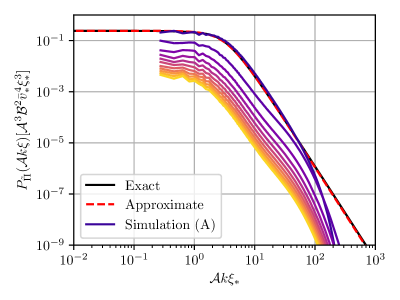
Figure 11: Anisotropic stress spectral density $P_{\tilde{\Pi}}(k,\tau_{*})$ at the initial time in the constant source approximation, from the exact integration of Eq. 7.13 (black solid line) and the analytical approximation Eq. 7.14 (red dashed line). We also show $P_{\tilde{\Pi}}(k,\tau)$ extracted from simulation (A) (colored solid lines) between $\tau=\tau_{*}$ and $\tau=\tau_{\mathrm{end}}$ with interval $\Delta\tau=9.96\tau_{\xi_{*}}$. Lighter colours indicate later times.

We now turn to the description of the anisotropic stress spectral density at initial time $P_{\tilde{\Pi}}(k,\tau_{*})$, also entering Eq. 7.8. This is given by the convolution in momentum of Eq. 2.24 (without residual time dependence). It takes the form (we use the notation of Appendix B):

$$P_{\tilde{\Pi}}(k,\tau_{*}) =\frac{\pi^{2}}{2}\mathcal{A}^{3}{\xi_{*}^{3}}\int_{0}^{\infty}\differential H\,H^{2}\int_{0}^{1}\differential\alpha\,\frac{\mathrm{Proj}(H,\alpha)}{\mathrm{s}^{3}(H,\alpha)\mathrm{s}^{3}(H,-\alpha)}\mathcal{P}_{v}[\mathrm{s}(H,\alpha),\tau_{*}]\mathcal{P}_{v}[\mathrm{s}(H,-\alpha),\tau_{*}]$$ (7.13)

$$\simeq\frac{P_{\tilde{\Pi}}(0)}{1+\quantity(\frac{\mathcal{A}k\xi_{*}}{3.0})^{2}+\quantity(\frac{\mathcal{A}k\xi_{*}}{3.5})^{11/3}}\,,$$ (7.14)

where the factors of $3.0$ and $3.5$ come from an analytical fit, tuned to match the exact numerical integration of Eq. 7.13, and $P_{\tilde{\Pi}}(0)$ is the value of the anisotropic stress spectral density at $k=0$:

$$P_{\tilde{\Pi}}(0)=\mathcal{B}^{2}\mathcal{A}^{3}\,\overline{v}_{*}^{4}\,{\xi_{*}^{3}}\int_{0}^{\infty}\differential{H}\frac{1024\,\sqrt[3]{2}\,\pi^{2}H^{6}}{(4H^{2}+4)^{17/3}}\int_{0}^{1}\differential{\alpha}(\alpha^{2}+1)^{2}=\mathcal{B}^{2}\mathcal{A}^{3}\,\overline{v}_{*}^{4}\,{\xi_{*}^{3}}\,\,\frac{7\pi^{5/2}\,\Gamma\left(\frac{13}{6}\right)}{8\,\Gamma\left(\frac{17}{3}\right)}\,.$$ (7.15)

In Fig. 11, we compare the anisotropic stress spectral density from simulation (A) with both the numerical result Eq. 7.13, and the analytical approximation Eq. 7.14. As can be appreciated from the figure, at the initial time $\tau_{*}$ there is excellent agreement between the simulation result and the anisotropic stress spectral density derived in the context of our turbulent model. For illustration purposes, in Fig. 11 we also display the time evolution of the anisotropic stress spectral density from simulation (A): it is decaying, due in turn to the decay of the turbulent source itself.

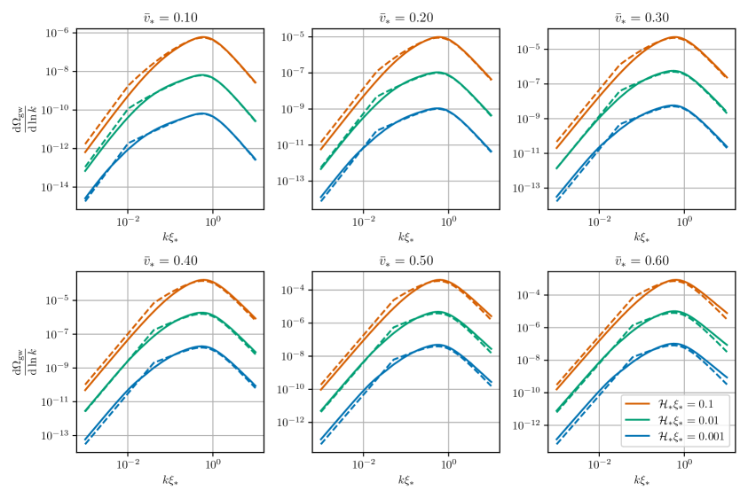
Figure 12: Reproduction of Fig. 10, where here we also show the constant source approximation given in Eq. 7.16 for different values of $\overline{v}_{*}$ and $\mathcal{H}_{*}\xi_{*}$. The solid lines match those of Fig. 10 (with $\beta=3$), whereas the dashed lines give the constant source approximation for an equivalent value of $\overline{v}_{*}$ and $\mathcal{H}_{*}\xi_{*}$. We fix $\mathcal{N}_{\mathrm{cut}}=7$ in the constant source approximation Eq. 7.16 for all values of $\overline{v}_{*}$ and $\mathcal{H}_{*}\xi_{*}$.

The spectral shape of the SGWB from a constant source, Eq. 7.8, is given by the combination of the $k$-dependence coming from both $\mathcal{T}_{\mathrm{gw}}(k,\tau_{*},\mathcal{N}_{\mathrm{cut}}\tau_{\xi_{*}})$ and $P_{\tilde{\Pi}}(k,\tau_{*})$. Recalling that the values of $\mathcal{A}$ and $\mathcal{B}$ can be found in Eqs. 3.14 and 3.15, we find

$$\derivative{{\Omega}_{\mathrm{gw}}}{\ln k}=\frac{7\sqrt{\pi}\,\Gamma(13/6)}{3\Gamma(17/3)}\frac{(\mathcal{A}\,k\,\xi_{*})^{3}\mathcal{B}^{2}\,\overline{v}_{*}^{4}}{1+\quantity(\mathcal{A}\,k\,\xi_{*}/3.0)^{2}+\quantity(\mathcal{A}\,k\,\xi_{*}/3.5)^{11/3}}\\ \times\begin{cases}\ln^{2}\quantity(1+\mathcal{N}_{\mathrm{cut}}\tau_{\xi_{*}}\mathcal{H}_{*})&\text{ for}~{}\sqrt{2}k<1/(\mathcal{N}_{\mathrm{cut}}\tau_{\xi_{*}})\\ \ln^{2}\quantity[1+\mathcal{H}_{*}/(\sqrt{2}\,k)]&\text{ for}~{}\sqrt{2}\,k>1/(\mathcal{N}_{\mathrm{cut}}\tau_{\xi_{*}})\end{cases}\text{.}$$ (7.16)

The $k$-dependence of $\mathcal{T}_{\mathrm{gw}}(k,\tau_{*},\mathcal{N}_{\mathrm{cut}}\tau_{\xi_{*}})$ has been described in Ref. [77] in the context of coherent sources, meaning those for which the UETC can be factorized. Eq. 7.10 is effectively a time-domain Fourier cosine transform, therefore the decay properties of $\mathcal{T}_{\mathrm{gw}}(k,\tau_{*},\mathcal{N}_{\mathrm{cut}}\tau_{\xi_{*}})$ at large $k$ depend on its time differentiability – and in the case being studied here, it is discontinuous in time. This gets combined with the behaviour of $P_{\tilde{\Pi}}(k,\tau_{*})$, which is uncorrelated for wavenumbers $k<1/(\mathcal{A}\xi_{*})$, while at high $k$ it shares the same power-law decrease as $P_{v}(k,\tau_{*})$ (hence, for an initially von Kármán spectrum, it decreases as $k^{-11/3}$ at high $k$) [20]. Altogether, for instantaneous turbulence generation of a von Kármán spectrum, the expected slopes for low $\overline{v}_{*}$ are (with notation $K=\mathcal{A}\xi_{*}k$):

$$\text{if}~{}~{}\mathcal{N}_{\mathrm{cut}}\mathcal{H}_{*}\xi_{*}<\overline{v}_{*}\,,\qquad \derivative{{\Omega}_{\mathrm{gw}}}{\ln k}\propto\begin{cases}\mathcal{N}_{\mathrm{cut}}^{2}\,\overline{v}_{*}^{2}\,(\mathcal{H}_{*}\xi_{*})^{2}\,K^{3}&\text{ for}~{}\mathcal{N}_{\mathrm{cut}}K\ll\overline{v}_{*}\,,\\ \overline{v}_{*}^{4}\,(\mathcal{H}_{*}\xi_{*})^{2}\,K^{1}&\text{ for}~{}\overline{v}_{*}\ll\mathcal{N}_{\mathrm{cut}}K\text{ and }K\ll 1\,,\\ \overline{v}_{*}^{4}\,(\mathcal{H}_{*}\xi_{*})^{2}\,K^{-8/3}&\text{ for}~{}1\ll K\,,\end{cases}$$ (7.17)

$$\text{if}~{}~{}\mathcal{N}_{\mathrm{cut}}\mathcal{H}_{*}\xi_{*}>\overline{v}_{*}\,,\qquad \derivative{{\Omega}_{\mathrm{gw}}}{\ln k}\propto\begin{cases}\overline{v}_{*}^{4}K^{3}\ln^{2}\quantity(1+\mathcal{N}_{\mathrm{cut}}\mathcal{H}_{*}\xi_{*}/\overline{v}_{*})&\text{ for}~{}\mathcal{N}_{\mathrm{cut}}K\ll\overline{v}_{*}\,,\\ \overline{v}_{*}^{4}K^{3}\ln^{2}\quantity[1+\mathcal{A}\mathcal{H}_{*}\xi_{*}/(\sqrt{2}\,K)]&\text{ for}~{}\overline{v}_{*}/\mathcal{N}_{\mathrm{cut}}\ll K\ll\mathcal{A}\mathcal{H}_{*}\xi_{*}\,,\\ \overline{v}_{*}^{4}\,(\mathcal{H}_{*}\xi_{*})^{2}\,K^{1}&\text{ for}~{}\mathcal{A}\mathcal{H}_{*}\xi_{*}\ll\mathcal{N}_{\mathrm{cut}}K\text{ and }K\ll 1\,,\\ \overline{v}_{*}^{4}\,(\mathcal{H}_{*}\xi_{*})^{2}\,K^{-8/3}&\text{ for}~{}1\ll K\,.\end{cases}$$ (7.18)

This behaviour is in accordance with that found in Refs. [77, 46]. Note that the $P_{\tilde{\Pi}}/k^{2}$ slope observed in Ref. [91] at high $k$ can be interpreted in light of what has been discussed above as well as the results of Ref. [77].

In Fig. 12, we plot the constant source approximation, Eq. 7.16, and compare it to the result of the full numerical integration presented in Section 5. As discussed above, we set $\mathcal{N}_{\mathrm{cut}}=7$ to match the SGWB spectra obtained from the numerical integration. The spectral shapes of the SGWBs evaluated under the constant source approximation are in good agreement with those produced with the numerical integration, over the tested range of values for the input parameters $\overline{v}_{*}$ and $\mathcal{H}_{*}\xi_{*}$. The discrepancy around the transition between regimes at $k=1/(\sqrt{2}\mathcal{N}_{\mathrm{cut}}\tau_{\xi_{*}})$, see Eq. 7.16, is most notable for sources that last longer than one Hubble time (meaning $\mathcal{N}_{\mathrm{cut}}\tau_{\xi_{*}}\mathcal{H}_{*}>1$), where the intermediate power law for wavenumbers smaller than the peak is less pronounced. Note that in Ref. [46] it was possible to adjust the source duration (i.e. the value of $\mathcal{N}_{\mathrm{cut}}$) in the constant approximation, as a function of $\overline{v}_{*}$ and $\mathcal{H}_{*}\xi_{*}$. This was done by comparison with the SGWBs output by the simulations, which covered also the large scale part of the spectrum. Here, on the other hand, we fix $\mathcal{N}_{\mathrm{cut}}=7$ for all initial $\overline{v}_{*}$ and $\mathcal{H}_{*}\xi_{*}$.

The UETC of decaying turbulence Eq. 4.7 has both a factorizable (coherent) component and a decorrelating one. The coherent component shapes the SGWB spectrum at large scales and around the peak. On the other hand, the decorrelation influences the spectral shape at small scales, as discussed in Section 7.1. The discrepancy that can be observed in Fig. 12 at high wavenumber for large $\overline{v}_{*}$ can therefore be interpreted in light of what found under the assumption of a purely stationary source, see the asymptotic behaviour at high $k$ of Eq. 7.6. The constant source approximation, in which the decorrelation is absent, predicts a steeper power law – given in Eq. 7.17 – than that found by the numerical integration, which contains the full time evolution of the source.

All in all, it emerges that both the overall decay of turbulence as well as its decorrelation play a relatively minor role in shaping the SGWB signal: the first influences the spectral shape only at large scales $k\xi_{*}<\overline{v}_{*}/\mathcal{N}_{\mathrm{e}}$, while the second does so only for large initial velocity $\overline{v}_{*}$ and at small scales $k\xi_{*}\gg 1$.

7.2.4 Comparison of the SGWB spectra

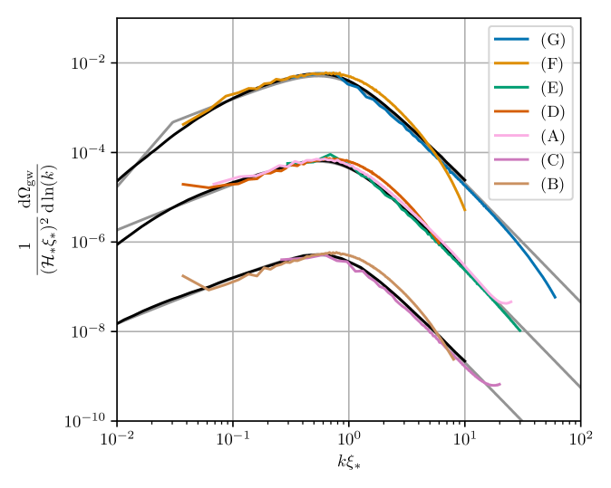
Figure 13: GW power spectrum for instantaneous turbulence generation. The gray lines show the analytical approximation of Eq. 7.16 based on a constant source lasting for $\mathcal{N}_{\mathrm{cut}}=7$ eddy turnover times. The black lines show the result of the 4d numerical integration of Section 7.2.2. From top to bottom, these lines correspond to $\overline{v}_{*}=0.3$, $\overline{v}_{*}=0.1$ and $\overline{v}_{*}=0.03$ respectively. In all cases we fix $\mathcal{H}_{*}\xi_{*}=0.001$. We also show the averaged GW power spectra for simulations (A)-(G) from Table 2, which are plotted using colored lines as specified in the legend. The GW power spectra from simulations has been cut off at high wavenumbers due to numerical precision noise.

In Sections 7.2.1, 7.2.2 and 7.2.3, we have presented three different methods of estimating the GW power spectrum when turbulence is generated instantaneously. We first presented the GW spectra from simulations, then we performed an exact numerical integration and finally computed an analytical approximation assuming a constant source.

In this section, we compare the GW spectra obtained from the three different methods. The comparison is performed (i) long after the source has dissipated and (ii) for the lowest value of $\mathcal{H}_{*}\xi_{*}$ for which we performed the numerical integration, namely $\mathcal{H}_{*}\xi_{*}=10^{-3}$. Condition (i) is necessary to perform the time average, while condition (ii) is necessary since the simulations neglect the effect of expansion. For more detail, we refer the reader to the discussions at the end of Sections 5.5 and 7.2.2.

We plot the late-time averaged GW power spectra from our simulations in Fig. 13, and compare them to those computed in the full numerical integration and in the constant source approximation. We show the GW power spectra from the numerical integration and the constant source approximation for $\overline{v}_{*}=0.03\text{,}~{}0.1$ and $0.3$. There is excellent agreement between the SGWBs obtained with the three methods, for all the values of $\overline{v}_{*}$ we simulated. They are all consistent with respect to the GW power spectrum amplitude, the breadth of the peak, the peak location at $k\xi_{*}\simeq 2.7/\mathcal{A}$ and the power laws at low and high wavenumbers. In particular, they all agree in the regions we expect the simulations to be accurate, namely at low wavenumbers for simulations (B), (D) and (F), and at high wavenumbers for simulations (C), (E) and (G). Simulation (A), which is our largest simulation, has close agreement with the other methods for the full range of wavenumbers depicted. We have therefore validated that the numerical integration and the constant approximation are accurate in the limit of $\mathcal{H}_{*}\xi_{*}\ll 1$. Furthermore, as they include the effect of expansion, we expect them to also be accurate outside this limit. As discussed in the previous section and depicted in Fig. 12, there is a discrepancy between the constant source approximation and the full numerical integration for wavenumbers close to the kink at $k=1/(\sqrt{2}\mathcal{N}_{\mathrm{cut}}\tau_{\xi_{*}})$. This can also be seen in Fig. 13.

As the constant source approximation displays excellent agreement around the peak and obtains the correct asymptotic power laws, Eq. 7.16 can be used as a simple approximation to the GW power spectrum which does not require simulations.

7.3 Phase of turbulence growth: results from the numerical integration

Figure 14: Diagram for the evolution of turbulence in terms of $\eta$ and $\zeta$. The injection of kinetic energy starts at $\tau_{\mathrm{ini}}$ and turbulence develops in region $1$ on a timescale $\tau_{\mathrm{gro}}$, the value of which depends on the model: it might correspond to the PT duration $\beta^{-1}$, or to the eddy turnover time $\tau_{\xi_{*}}$. In region $2$, the turbulence is freely decaying. The growth and free decay phases are correlated: regions $3$ and $4$ also contribute to the production of GWs.

In this section we go beyond the scenario of instantaneous turbulence generation, considered so far, and include a growth phase for the turbulence kinetic energy. Since the Reynolds number in the early Universe is very large (of the order of $10^{13}$ at the electroweak scale, see Section 7.2.2), turbulence is expected to arise from vorticity generated during the PT [16], or due to the interaction of shocks [29, 30]. In order to model the GW source properly, one would have to model the onset of turbulence by simulating the complete system of scalar field and fluid. We leave this complicated problem for future work.

In the present analysis we model the (purely vortical) turbulence growth phase heuristically. This allows us to gauge in a simple way the importance of this phase, as far as the SGWB spectral shape is concerned. Refs. [77, 36, 37] have demonstrated analytically that time continuity of the GW sourcing process must be ensured, since it plays a role in shaping the SGWB signal, and Refs. [42, 92, 93] also obtained different SGWB spectral shapes in the forced case. As we shall see, we confirm this result in the present work, via the numerical integration of the SGWB source (see Section 7.2.2).

Starting from the initial time $\tau_{\mathrm{ini}}$, we assume that turbulence is sourced on a timescale $\tau_{\mathrm{gro}}$. At time $\tau_{*}=\tau_{\mathrm{ini}}+\tau_{\mathrm{gro}}$, turbulence is fully developed, and then starts decaying (see Fig. 14). The duration of the growth phase would depend on the particular mechanism sourcing the turbulence. If the sourcing process is related to the PT dynamics, one would expect the duration of the growth phase to be of the order of the duration of the PT. Alternatively, one can assume that it takes approximately one initial eddy turnover time $\tau_{\xi_{*}}=\xi_{*}/\overline{v}_{*}$ to build the turbulent cascade. This is the assumption we make in the following, namely that $\tau_{\mathrm{gro}}=\tau_{\xi_{*}}$.

Concerning the correlations of the velocity field, the Gaussian decorrelation scenario of Sections 3.3.1 and 4.2 holds in principle only in the free-decay phase. However, in the absence of a better model, we assume that Eq. 4.7 is valid also during the growth phase, and in the mixed regions. Therefore, in the UETC of Eq. 4.7, the times $\tau$ and $\zeta$ can pertain either both to the growth phase, or both to the free decay phase, or to the two phases mixed (see Fig. 14).

We consider two scenarios for the generation of turbulence: a $\mathcal{C}^{0}$ growth phase and a $\mathcal{C}^{1}$ growth phase. First we adopt the model of Ref. [37] and suppose that the vortical kinetic energy grows linearly in time before turbulence enters the free-decay phase. Furthermore, we assume that the integral scale remains constant during the growth phase, and starts growing during the phase of free decay in the $\mathcal{C}^{0}$ scenario:

$$\begin{split}\overline{v}^{2}(\tau)&=\overline{v}_{*}^{2}\begin{cases}\dfrac{\tau-\tau_{\mathrm{ini}}}{\tau_{\mathrm{gro}}}&\text{if }\tau<\tau_{*}\\ \quantity(\dfrac{\tau-\tau_{*}+\mathcal{N}_{\mathrm{e}}\tau_{\xi_{*}}}{\mathcal{N}_{\mathrm{e}}\tau_{\xi_{*}}})^{-p}&\text{if }\tau>\tau_{*}\end{cases}\\ \text{and}\quad\xi(\tau)&=\xi_{*}\begin{cases}1&\text{if }\tau<\tau_{*}\\ \quantity(\dfrac{\tau-\tau_{*}+\mathcal{N}_{\mathrm{e}}\tau_{\xi_{*}}}{\mathcal{N}_{\mathrm{e}}\tau_{\xi_{*}}})^{q}&\text{if }\tau>\tau_{*}.\end{cases}\end{split}$$ (7.19)

In the second scenario the kinetic energy and the integral scale evolve in such a way that they are both continuous and differentiable at time $\tau_{*}$. The kinetic energy is also continuous and differentiable at initial time $\tau_{\mathrm{ini}}$. This scenario requires defining two extra functions. For the growth phase of the kinetic energy we use a smooth step function with the properties $\operatorname{SStep}(1)=1$, $\operatorname{SStep}^{\prime}(1)=0$ (and also, $\operatorname{SStep}(0)=\operatorname{SStep}^{\prime}(0)=0$):

$$\operatorname{SStep}(x)=\begin{cases}0&x<0\\ 3x^{2}-2x^{3}&0<x<1\\ 1&x>1.\end{cases}$$ (7.20)

To connect with the decay phase, we use a smooth power law with the property $\operatorname{SPL}(1,p)=1$ and $\operatorname{SPL}^{\prime}(1,p)=0$:

$$\operatorname{SPL}(x,p)=(1-p)x^{p}+px^{p-1}\,,$$ (7.21)

where $p<1$. Using the above functions, we set for the $\mathcal{C}^{1}$ scenario:

$$\begin{split}\overline{v}^{2}(\tau)&=\overline{v}_{*}^{2}\begin{cases}\operatorname{SStep}\quantity(\dfrac{\tau-\tau_{\mathrm{ini}}}{\tau_{\mathrm{gro}}})&\text{if }\tau<\tau_{*}\\ \operatorname{SPL}\quantity(\dfrac{\tau-\tau_{*}+\mathcal{N}_{\mathrm{e}}\tau_{\xi_{*}}}{\mathcal{N}_{\mathrm{e}}\tau_{\xi_{*}}},-p)&\text{if }\tau>\tau_{*}\end{cases}\\ \text{and}\quad\xi(\tau)&=\xi_{*}\begin{cases}1&\text{if }\tau<\tau_{*}\\ \operatorname{SPL}\quantity(\dfrac{\tau-\tau_{*}+\mathcal{N}_{\mathrm{e}}\tau_{\xi_{*}}}{\mathcal{N}_{\mathrm{e}}\tau_{\xi_{*}}},q)&\text{if }\tau>\tau_{*}.\end{cases}\end{split}$$ (7.22)

Different choices for the growth phase lead to different spectral shapes in the resulting SGWB. This is demonstrated by Fig. 15, showing the SGWB with both the $\mathcal{C}^{0}$ and $\mathcal{C}^{1}$ growth phases, as well as for the instantaneous generation scenario. While the spectra at large scales are comparable, inserting a continuous growth phase shifts the spectral peak position from the characteristic length scale of the source, $k_{\mathrm{peak}}\simeq\xi_{*}^{-1}$, to the characteristic timescale of the source, $k_{\mathrm{peak}}\simeq\tau_{\xi_{*}}^{-1}$: the peak position becomes therefore velocity-dependent [77]. This behaviour is caused by the component in the velocity field UETC Eq. 4.7 which is factorizable in time, termed the “coherent” case in Ref. [77]; see the discussion below Eq. 7.16. Furthermore, the addition of a growth phase which is continuous in time leads to a reduction in the GW power, and a steeper slope at high frequencies, as shown in Fig. 16 (in this figure we only plot the results for the $\mathcal{C}^{1}$ growth phase). Since the peak now corresponds to the inverse eddy turnover time, the $k^{1}$ region observed in the instantaneous growth scenario never develops, as illustrated by Fig. 15. Note that the spectra in the $\mathcal{C}^{0}$ and $\mathcal{C}^{1}$ growth phase are almost identical, contrary to what was observed in Ref. [77]. Indeed, we would not expect Ref. [77] to capture all the complexity of the spectral changes due to the insertion of a continuous growth phase, since it studied a very simplified case in which the anisotropic stress UETC was separable in time.

At first, it may seem counter-intuitive that the addition of a growth phase decreases the energy in GWs, given Mercer’s condition (see Section 4.1). We illustrate this using Fig. 14: Mercer’s condition Eq. 4.2 applies to intervals of the form $I\times I$, hence the contributions from the regions $1$ and $2$ are positive. However, the contributions from the regions $3$ and $4$ can very well be negative, lowering the total GW energy. This effect depends crucially on the correlations between the growth and the free decay phase. We leave the study of the growth of turbulence from more realistic initial conditions to a future work.

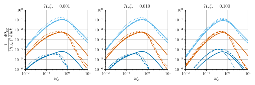
Figure 15: Gravitational wave power spectrum in the instantaneous generation scenario (solid lines), with a $\mathcal{C}^{0}$ growth phase (dashed lines) and with a $\mathcal{C}^{1}$ growth phase (dotted lines). From bottom to top, $\overline{v}_{*}=0.1,0.3$ and $0.6$. The left panel shows $\mathcal{H}_{*}\xi_{*}=10^{-3}$, the middle panel $\mathcal{H}_{*}\xi_{*}=10^{-2}$ and the right panel $\mathcal{H}_{*}\xi_{*}=10^{-1}$.

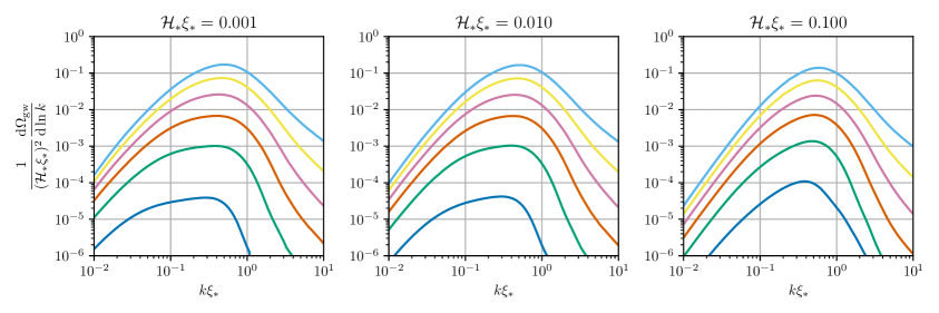
Figure 16: Gravitational wave power spectrum in the scenario with $\mathcal{C}^{1}$ growth phase. Each panel displays a different value for the initial integral scale $\mathcal{H}_{*}\xi_{*}$ (as specified in the panels titles), and each line corresponds to $\overline{v}_{*}=0.1,0.2,0.3,0.4,0.5,$ and $0.6$ from bottom to top.

8 Discussion

In this paper, we have studied the GW signal generated by a phase of freely decaying vortical turbulence in a relativistic fluid. We were motivated by the fact that thermal first order phase transitions occurring in the early Universe are expected to lead to a turbulent flow, either directly from vorticity generation during bubble collisions, or from the interaction of shocks following the acoustic phase. Since the sourcing of the turbulent flow remains an active area of research, we have chosen to focus on GW production in the phase of turbulent free decay, inserting as our initial conditions a fully developed turbulent spectrum, as if the turbulence generation was instantaneous. While this is not the most realistic assumption, it simplified our analysis, allowing us to build a thorough understanding of the temporal and spatial structure of both the velocity field and the subsequent GW signal. We thereby derived a model for the UETC of the velocity field in freely decaying turbulence. The GW source, built in the context of this model, was then integrated to compute the GW spectrum. The validity of our model and of the integration technique was supported with a series of simulations using the Minkowski space relativistic hydrodynamics code SCOTTS. The simulations were prepared with equivalent initial conditions to our model, namely a fully developed turbulent spectrum.

The velocity of the turbulent fluid was assumed to follow the von Kármán power spectrum, interpolating between a causal $k^{5}$ slope at low wavenumbers and a Kolmogorov $k^{-2/3}$ one at high wavenumbers. This basic choice influences the spectral shape of the anisotropic stress power spectrum and consequently of the GW power spectrum. Concerning the velocity UETC, motivated by the Kraichnan sweeping model, we assumed that the velocity field decorrelation is Gaussian in time, with a timescale set by the Eulerian eddy turnover time. We implemented the decorrelation at larger scales, around the spectral peak, by extending the decorrelation velocity according to Ref. [39]. We further addressed the modelling of decorrelation in the context of the theory of positive kernels, and propose to model the UETC of the turbulent velocity field as a Gibbs kernel. This both consistently enforces time symmetry in the UETC, and guarantees that the GW power spectrum is non-negative. We have validated our model for the velocity field decorrelation with a series of relativistic hydrodynamic simulations performed with SCOTTS, with the initial root-mean-squared velocity, $\overline{v}_{*}$, ranging from $0.03$ to $0.3$. We used our simulations also to study the time evolution of both the kinetic energy and the integral scale, allowing us to fix the number of eddy turnover times that it takes for the turbulence to decay.

We have reviewed the analytical computation of the SGWB from a purely vortical fluid, arriving at an equation for the GW power spectrum in terms of an integral over the Green’s function and the anisotropic stress UETC, which is provided by the turbulence model we have developed. The computation of the GW spectrum could then be performed without any further approximation using Monte Carlo integration with importance sampling. Varying the exponents of the turbulence decay laws had limited impact on the resulting GW spectrum. We therefore conclude that our predictions are robust with respect to this unknown. For instantaneously generated turbulence, we found excellent agreement between the GW signal evaluated with direct numerical integration and the one extracted from our simulations.

To conclude our exploration of the GW signal in instantaneously generated turbulence, we studied the case of a turbulent source which is constant in time. As the GW spectrum at high wavenumbers and around the peak is built up on short timescales in comparison to the decay of the source, the constant source approximation works well in this region. The GW power spectrum derived within the constant source approximation is in very good agreement with both the simulation result and the power spectrum arising from direct numerical integration of the turbulence model we have built. We provide an analytical form for the SGWB signal from turbulence, Eq. 7.16, which has the advantage that it can be readily used without the need to perform simulations or the challenging computation of 4-dimensional integrals.

Finally, we explored how the GW spectrum was modified by inserting a growth phase for the turbulence, therefore removing the time discontinuity inherent in the instantaneous generation assumption. We considered in particular a $\mathcal{C}^{0}$ growth phase and a $\mathcal{C}^{1}$ growth phase. These models, although simplistic, allowed us to show how the GW signal might be modified by the turbulence generation phase. In contrast to the decay law exponents, the form of the initial growth phase has a large effect on the GW power spectrum: flows with equivalent $\overline{v}_{*}$ can lead to GW signals with different spectral shapes and amplitudes, if the initial condition differs. This underlines the importance of understanding the turbulence formation mechanism in the context of first order phase transitions.

Future works will therefore focus on the generation of turbulence — which we showed is crucial to make precise predictions for future GW experiments — and on the inclusion of the longitudinal velocity field and a magnetic field.

Appendix A Integration variables for the evaluation of the GW power spectrum

Figure 17: Coordinate system consisting of $(h,\alpha)$.

This appendix summarizes the changes of variable we perform in order to tackle the convolution integral $\differential[3]{p}$ in Eq. 7.1. To make the symmetries of the integrand apparent, we first set $\mathbf{h}=\mathbf{p}-\mathbf{k}/2$, see Fig. 17. Denoting $\alpha=\hat{\mathbf{k}}\dotproduct\hat{\mathbf{h}}$, it follows that

$$p^{2}=\absolutevalue{\mathbf{k}/2+\mathbf{h}}^{2} =k^{2}/4+hk~{}\alpha+h^{2}\equiv\mathrm{s}^{2}(h,\alpha)$$ (A.1)

$$\absolutevalue{\mathbf{k}-\mathbf{p}}^{2}=\absolutevalue{\mathbf{k}/2-\mathbf{h}}^{2} =k^{2}/4-hk~{}\alpha+h^{2}\equiv\mathrm{s}^{2}(h,-\alpha)\,.$$ (A.2)

The projection factor becomes (note the symmetry $\alpha\rightarrow-\alpha$)

$$\quantity[1+(\hat{\mathbf{k}}\dotproduct\hat{\mathbf{p}})^{2}]\quantity[1+(\hat{\mathbf{k}}\dotproduct\widehat{\mathbf{k-p}})^{2}] = 4\quantity[1-\frac{h^{2}(1-\alpha^{2})}{2(k^{2}/4-hk~{}\alpha+h^{2})}]\quantity[1-\frac{h^{2}(1-\alpha^{2})}{2(k^{2}/4+hk~{}\alpha+h^{2})}]$$ (A.3)

$$\equiv \mathrm{Proj}(h,\alpha).$$

For the numerical integration, it is useful to define the new variable $M\equiv{k^{2}}/(k^{2}+h^{2})$. The volume element of the spherical coordinates $(h,\theta,\phi)$ can then be written as

$$\differential[3]{h}=\frac{k\differential{M}}{2\sqrt{1-M}M^{3/2}}\differential{\alpha}\differential{\phi}$$ (A.4)

with $M\in]0,1]$ and $\alpha\in[0,1]$. Note that the integrand in Eq. 7.1 is invariant under rotations of the azimuthal angle $\phi$.

Appendix B Analytical expressions for the stationary assumption

Under the stationary assumption, whose implications are described in Section 7.1, Eq. 7.4 can be rewritten as:

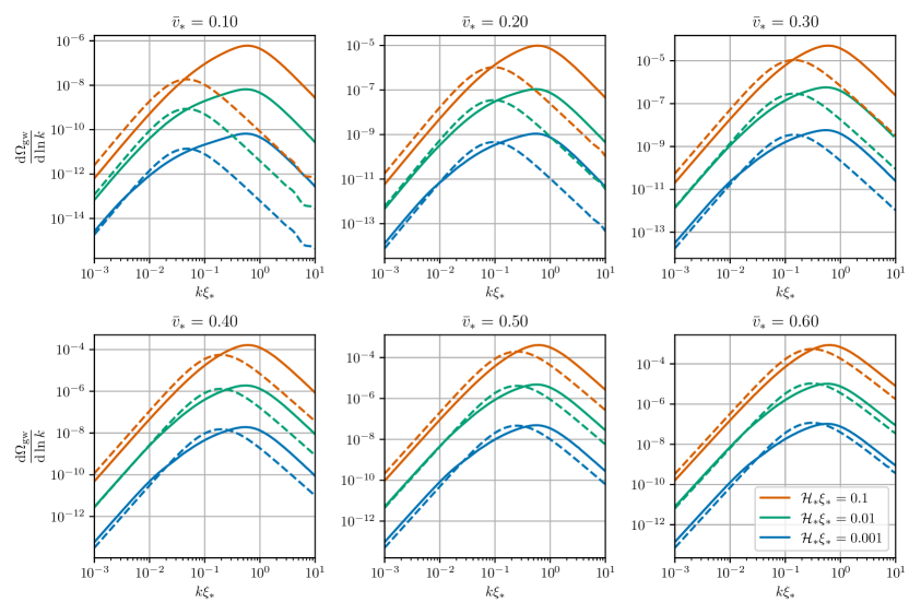
Figure 18: As in Fig. 10, we show the SGWB spectra for several values of $\overline{v}_{*}$ and $\mathcal{H}_{*}\xi_{*}$ in the instantaneous generation scenario with $\beta=3$ (solid lines), compared with the SGWB obtained within the stationary assumption given in Eq. B.4 (dashed lines). We fix $\mathcal{N}_{\mathrm{cut}}=7$ as in the constant source approximation, see Eq. 7.8.

$$\derivative{{\Omega}_{\mathrm{gw}}}{\ln k}= \frac{4}{3}k^{3}\int_{0}^{\infty}\differential h\,h^{2}\int_{0}^{1}\differential\alpha\,\frac{\mathrm{Proj}(h,\alpha)}{\mathrm{s}^{3}(h,\alpha)\mathrm{s}^{3}(h,-\alpha)}\mathcal{P}_{v}[\mathrm{s}(h,\alpha)]\mathcal{P}_{v}[\mathrm{s}(h,-\alpha)]$$

$$\times\Bigg{\{}\int_{\tau_{*}}^{\frac{\tau_{*}+\tau_{\mathrm{fin}}}{2}}\differential\tau_{\mathrm{mid}}\int_{0}^{2\tau_{\mathrm{mid}}-2\tau_{*}}\differential\tau_{\mathrm{diff}}\,\frac{\cos(k\tau_{\mathrm{diff}})}{\tau_{\mathrm{mid}}^{2}-\frac{\tau_{\mathrm{diff}}^{2}}{4}}\exp\quantity[-\frac{\overline{v}_{*}^{2}\tau_{\mathrm{diff}}^{2}}{3}\quantity(h^{2}+\frac{k^{2}}{4})]$$

$$+\int_{\frac{\tau_{*}+\tau_{\mathrm{fin}}}{2}}^{\tau_{\mathrm{fin}}}\differential\tau_{\mathrm{mid}}\int_{0}^{2\tau_{\mathrm{fin}}-2\tau_{\mathrm{mid}}}\differential\tau_{\mathrm{diff}}\,\frac{\cos(k\tau_{\mathrm{diff}})}{\tau_{\mathrm{mid}}^{2}-\frac{\tau_{\mathrm{diff}}^{2}}{4}}\exp\quantity[-\frac{\overline{v}_{*}^{2}\tau_{\mathrm{diff}}^{2}}{3}\quantity(h^{2}+\frac{k^{2}}{4})]\Bigg{\}}\,,$$ (B.1)

where $\mathrm{s}(h,\alpha)$ and $\mathrm{Proj}(h,\alpha)$ are defined in Eqs. (A.1), (A.2) and (A.3) of Appendix A, and we have used Eq. 3.9 in Eq. 2.24 to express the power spectral density in terms of the power spectrum $\mathcal{P}_{v}[\mathrm{s}(h,-\alpha)]$, defined in Eq. 3.13. In order to proceed analytically, we make some extra assumptions: (i) we push the upper limit of the integration in $\differential\tau_{\mathrm{diff}}$ to $+\infty$; (ii) we neglect the term $\tau_{\mathrm{diff}}^{2}/4$ with respect to $\tau_{\mathrm{mid}}^{2}$ in the denominator of Eq. B.1. Indeed, since $\tau_{\mathrm{diff}}^{2}/4\leq\tau_{\mathrm{mid}}^{2}/4$, we expect that the Gaussian decorrelation favours the region $\tau_{\mathrm{diff}}^{2}\ll 1$ for the generation of GW. Under these assumptions, the 4 dimensional integration reduces to a 1 dimensional one. First, the integral over the time difference becomes

$$\int_{0}^{\infty}\cos(k\tau_{\mathrm{diff}})\exp[-\frac{\overline{v}_{*}^{2}\tau_{\mathrm{diff}}^{2}}{3}\quantity(h^{2}+\frac{k^{2}}{4})]\differential{\tau_{\mathrm{diff}}}=\frac{\sqrt{3\pi}}{\overline{v}_{*}\sqrt{k^{2}+4h^{2}}}\exp[-\frac{3k^{2}}{(k^{2}+4h^{2})\overline{v}_{*}^{2}}].$$ (B.2)

Additionally, the integral over absolute time starting at $\tau_{*}=\mathcal{H}_{*}^{-1}$ and lasting until $\tau_{\mathrm{fin}}=\tau_{*}+\mathcal{N}_{\mathrm{cut}}\tau_{\xi_{*}}$ where $\tau_{\xi_{*}}=\xi_{*}/\overline{v}_{*}$, gives

$$\int_{\tau_{*}}^{\tau_{*}+\mathcal{N}_{\mathrm{cut}}\tau_{\xi_{*}}}\frac{\differential{\tau_{\mathrm{mid}}}}{\tau_{\mathrm{mid}}^{2}}=\mathcal{H}_{*}\frac{\mathcal{N}_{\mathrm{cut}}\mathcal{H}_{*}\xi_{*}}{\overline{v}_{*}+\mathcal{N}_{\mathrm{cut}}\mathcal{H}_{*}\xi_{*}}.$$ (B.3)

Finally, it is possible to integrate analytically over $\alpha=\cos\theta$, yielding the GW power spectrum in terms of the 1-dimensional integration (we define $H=\mathcal{A}\xi h$ and $K=\mathcal{A}\xi k$)

$$\derivative{{\Omega}_{\mathrm{gw}}}{\ln k}=\frac{32\,2^{1/3}}{55}\sqrt{\frac{\pi}{3}}\,\mathcal{A}\,\mathcal{B}^{2}\,\frac{N\,(\mathcal{H}_{*}\xi_{*})^{2}}{\overline{v}_{*}+N\mathcal{H}_{*}\xi_{*}}\,\overline{v}_{*}^{3}\int_{0}^{\infty}\differential{H}\frac{H^{2}}{K\sqrt{4H^{2}+K^{2}}}\exp[-\frac{3K^{2}}{\overline{v}_{*}^{2}(4H^{2}+K^{2})}]f(H,K),$$ (B.4)

where the function $f(H,K)$ is given by

$$f(H,K)\equiv ~{}\frac{f_{1}}{\quantity(K^{2}+4H^{2}+4)^{17/3}}\,\phantom{}_{{}_{2}}\mathrm{F}\!_{{}_{1}}\!\left(\frac{1}{2},\frac{5}{6};\frac{3}{2};\frac{16K^{2}H^{2}}{K^{2}+4H^{2}+4}\right)$$ (B.5)

$$+\frac{3f_{2}}{\quantity(K^{2}+4H^{2}+4)^{4}\quantity(K^{4}-8K^{2}(H^{2}-1)+16(H^{2}+1)^{2})^{11/6}}$$

with

$$f_{1}\equiv~{} 16(415H^{2}+171)K^{6}+768(H^{2}+1)^{2}(5H^{2}+9)K^{2}+6912(H^{2}+1)^{4}$$ (B.6)

$$+32(305H^{4}+402H^{2}+225)K^{4}+1339K^{8}\,,$$

$$f_{2}\equiv~{} 8(613-247H^{2})K^{10}+18432(H^{2}-3)(H^{2}+1)^{4}K^{2}-36864(H^{2}+1)^{6}+$$ (B.7)

$$16(-823H^{4}+1042H^{2}+121)K^{8}+256(H^{2}+1)^{2}(361H^{4}-174H^{2}-231)K^{4}$$

$$+256(55H^{6}+73H^{4}-251H^{2}-141)K^{6}+727K^{12}\,.$$

Fig. 18 compares the SGWB obtained within the stationary assumption with the results of Section 7.2.2. Within the stationary assumption, the GW spectrum peaks at $k\simeq 2\overline{v}_{*}/(\mathcal{A}\xi_{*})$, while in the instantaneous generation scenario the peak occurs at $k\simeq 2.7/(\mathcal{A}\xi_{*})$. The stationary assumption also leads to a substantial reduction of power at small scales. In Section 7.1 we provide the low and high wavenumber asymptotic behaviour of the SGWB (B.4), for which the prefactors are

$$c_{1}=\frac{3\sqrt{3\pi}}{110}\mathcal{A}\,\mathcal{B}^{2}\simeq 0.3\,,\quad c_{2}=\frac{896\sqrt{\pi}}{405}\quantity(\frac{4}{3})^{\frac{1}{6}}\Gamma\quantity(\frac{8}{3})\mathcal{A}\,\mathcal{B}^{2}\simeq 23\,,\quad c_{3}=\frac{24\sqrt{6\pi}}{55}\mathcal{A}\,\mathcal{B}^{2}\Upsilon\simeq 57$$ (B.8)

where we have fit the factor $\Upsilon\simeq 8$.

Appendix C Finite volume tests

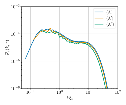
Figure 19: Velocity power spectra at $\tau=\tau_{\mathrm{end}}$ in simulations (A), ($\mathrm{A}^{\prime}$) and ($\mathrm{A}^{\prime\prime}$).

We performed two additional test simulations ($\mathrm{A}^{\prime}$) and ($\mathrm{A}^{\prime\prime}$) to understand how the low-wavenumber behaviour seen in simulation (A) depends on the cutoff induced by the box size. As shown in Table 2, these simulations have the same input power spectrum as simulation (A), but with different simulation volumes. By reducing the number of lattice points by a factor of 2 or 4 for simulation ($\mathrm{A}^{\prime}$) and ($\mathrm{A}^{\prime\prime}$) respectively, there is less dynamic range above the integral scale $\xi_{*}$. The small differences in $\overline{v}_{*}$ and $\xi_{*}$ are explained partially by the use of a different random seed and partially by the different simulation volume.

In Fig. 19 we plot the final velocity power spectra from each simulation. It can be seen that even by the end of the simulation, there is broad agreement between the simulations for the wavenumbers that they share in common. We plot the evolution of $\xi$ and $\overline{v}^{2}$ in each of the simulations in Fig. 20b. From this we can see that the evolution of the kinetic energy is relatively similar, however for ($\mathrm{A}^{\prime\prime}$) we see that the integral scale is unable to evolve to larger values due to the limited volume. Simulation $\mathrm{A}^{\prime}$) has a closer agreement with ($\mathrm{A}$) at early times, but still deviates at late times as the $\xi$ continues to grow.

This effect then modifies the rest of our global plots. In Fig. 21, we show the evolution of the instantaneous kinetic energy and integral scale exponents $(p,q)$, both parametrically and as a function of time. We see that the simulations agree on $p$ and $q$ at early times, but diverge in particular for the exponent $q$ at later times. This is unsurprising, as when $q$ is positive it indicates that the integral scale is growing. Eventually $\xi$ becomes comparable to the maximum scale within the simulation and the fluid flow becomes increasingly sensitive to the size of the box. At this point it appears the growth of $\xi$ is restricted, leading to a reduction in $q$.

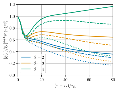
(a) Evolution of $\overline{v}^{2}\xi^{1+\beta}$

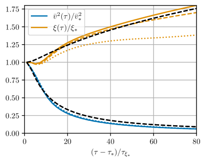
(b) Evolution of $\xi$ and $\overline{v}^{2}$

Figure 20: Left panel: Evolution of $\overline{v}^{2}\xi^{1+\beta}$ for different values of $\beta$ in simulations (A), ($\mathrm{A}^{\prime}$) and ($\mathrm{A}^{\prime\prime}$). As shown in the main text, this quantity should remain constant in freely decaying turbulence, thus indicating that $\beta\simeq 3$. Right panel: Evolution of the velocity and integral scale in simulations (A), ($\mathrm{A}^{\prime}$) and ($\mathrm{A}^{\prime\prime}$). The black-dashed line showcases Eqs. 3.21 and 3.22 for $\mathcal{N}_{\mathrm{e}}=5$, $p=4/3$ and $q=1/3$, where the values of $p$ and $q$ correspond to $\beta=3$. In both panels, the coloured solid lines refer to simulation (A), dashed lines to ($\mathrm{A}^{\prime}$) and dotted lines to ($\mathrm{A}^{\prime\prime}$).

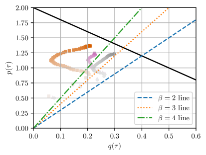
(a) Instantaneous exponents $(p,q)$.

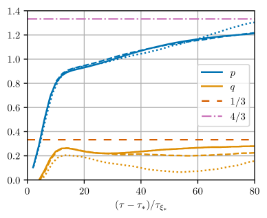
(b) Time evolution $p(\tau)$, $q(\tau)$.

Figure 21: Left panel: Trajectory of the instantaneous exponents $(p,q)$ in simulation (A), ($\mathrm{A}^{\prime}$) and ($\mathrm{A}^{\prime\prime}$). Simulation (A) is shown with circular gray markers, ($\mathrm{A}^{\prime}$) with pink triangles, and ($\mathrm{A}^{\prime\prime}$) with orange squares. Time is represented by the colour scheme: early times are shown with lighter shades and late times with darker shades, starting at $\tau=\tau_{*}$, with interval $\Delta\tau\sim 2\tau_{\xi_{*}}$. The dark solid line represents the self-similarity line $p=2(1-q)$. The coloured lines show the relation $p=(1+\beta)q$ for various choices of $\beta$. Right panel: Evolution of the instantaneous kinetic energy and integral scale exponents $(p,q)$ as a function of time in simulation (A), ($\mathrm{A}^{\prime}$) and ($\mathrm{A}^{\prime\prime}$). Solid lines refer to simulation (A), dashed lines to ($\mathrm{A}^{\prime}$) and dotted lines to ($\mathrm{A}^{\prime\prime}$). The horizontal lines show the values expected for $p$ and $q$ if $\beta=3$.

Appendix D Unequal time correlations in other simulations

In this appendix, we give the plots of the UETCs for simulations (B)-(C) in Fig. 22, simulations (D)-(E) in Fig. 23 and simulations (F)-(G) in Fig. 24. The $y$-axis is $D_{\mathrm{A}+}(k,\tau,\tau_{\mathrm{ref}})$.

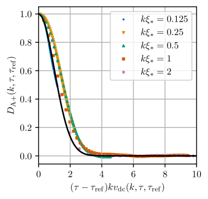
(a) Simulation (B).

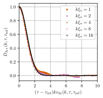
(b) Simulation (C).

Figure 22: Real part of the unequal time correlator measured in simulation (B) on the left panel and simulation (C) on the right panel. The $y$-axis displays $D_{\mathrm{A}+}(k,\tau,\tau_{\mathrm{ref}})$. The solid dark line is the prediction of our model combining Eqs. 3.33, 3.36 and 4.8.

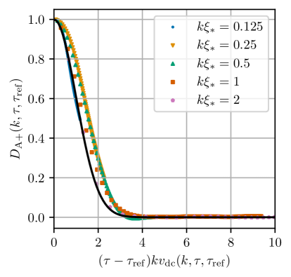
(a) Simulation (D).

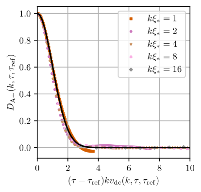
(b) Simulation (E).

Figure 23: Real part of the unequal time correlator measured in simulation (D) on the left panel and simulation (E) on the right panel. The $y$-axis displays $D_{\mathrm{A}+}(k,\tau,\tau_{\mathrm{ref}})$. The solid dark line is the prediction of our model combining Eqs. 3.33, 3.36 and 4.8).

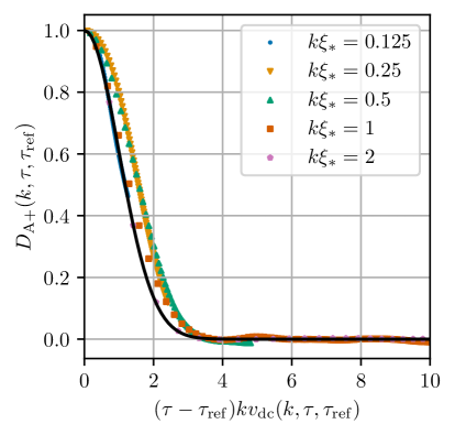
(a) Simulation (F).

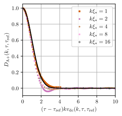
(b) Simulation (G).

Figure 24: Real part of the unequal time correlator measured in simulation (F) on the left panel and simulation (G) on the right panel. The $y$-axis displays $D_{\mathrm{A}+}(k,\tau,\tau_{\mathrm{ref}})$. The solid dark line is the prediction of our model combining Eqs. 3.33, 3.36 and 4.8).

Appendix E Other GW power spectra from simulations

In this appendix we present the plots of the GW power spectrum from simulations (B)-(C) with $\overline{v}_{*}\approx 0.03$ in Fig. 25, and (F)-(G) with $\overline{v}_{*}\approx 0.3$ in Fig. 26.

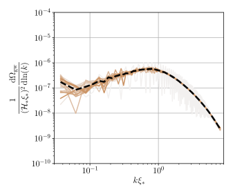
(a) Simulation (B), $\Delta\tau/\tau_{\xi_{*}}=4.97$.

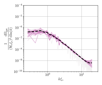
(b) Simulation (C), $\Delta\tau/\tau_{\xi_{*}}=0.647$.

Figure 25: GW power spectrum from simulations with $\overline{v}_{*}\approx 0.03$. The left and right panels show simulation (B) and (C) from Table 2 respectively. The coloured lines show the GW power spectrum with interval $\Delta\tau$ as listed in the caption, with darker shades corresponding to later times. The black dashed line shows an average over the GW power spectrum in the last $50\%$ of the simulation. We have cut off the spectrum at high wavenumbers due to numerical precision noise.

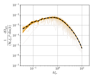
(a) Simulation (F), $\Delta\tau/\tau_{\xi_{*}}=5.16$.

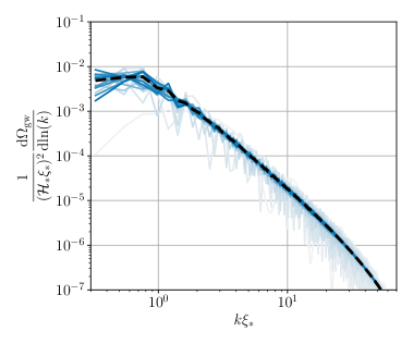
(b) Simulation (G), $\Delta\tau/\tau_{\xi_{*}}=0.583$.

Figure 26: GW power spectrum from simulations with $\overline{v}_{*}\approx 0.3$. The left and right panels show simulation (F) and (G) from Table 2 respectively. The coloured lines show the GW power spectrum with interval $\Delta\tau$ as listed in the caption, with darker shades corresponding to later times. The black dashed line shows an average over the GW power spectrum in the last $50\%$ of the simulation. We have cut off the spectrum at high wavenumbers due to numerical precision noise.

Appendix F Vortical and longitudinal velocity in simulations

In this work we assume that the velocity field is purely vortical. While the longitudinal component can be set to zero in the analytical modelling or during the numerical integration, in the numerical simulations a longitudinal component can in principle develop even if it is removed in the initial conditions. In the following short appendix, we present the evolution of the kinetic energy, $\overline{v}^{2}$, within the simulations, split into its vortical and longitudinal components. Note that in the following we adjust our notation to explicitly indicate both the longitudinal and vortical components of the velocity field.

We can decompose the spectral density into vortical and longitudinal components,

$$\expectationvalue{v_{i}(\mathbf{k},\tau)v_{j}^{*}(\mathbf{q},\tau)}\equiv(2\pi)^{3}\delta\quantity(\mathbf{k}-\mathbf{q})\left[\bot_{ij}(\hat{\mathbf{k}})P_{v_{\perp}}(k,\tau)+(1-\bot_{ij}(\hat{\mathbf{k}}))P_{v_{\parallel}}(k,\tau)\right]\text{.}$$ (F.1)

From these we can construct the vortical and longitudinal kinetic energy analogous to Eq. 3.8,

$$\overline{v}_{\perp/\parallel}^{2}(\tau)\equiv\int\frac{\differential k}{k}\mathcal{P}_{v_{\perp/\parallel}}(k,\tau)\text{,}$$ (F.2)

where the vortical and longitudinal power spectra are given by

$$\mathcal{P}_{v_{\perp/\parallel}}(k,\tau)=\frac{k^{3}}{\pi^{2}}P_{v_{\perp/\parallel}}(k,\tau)\text{,}$$ (F.3)

and the total kinetic energy is

$$\overline{v}^{2}(\tau)=\overline{v}^{2}_{\perp}(\tau)+\overline{v}_{\parallel}^{2}(\tau)\text{.}$$ (F.4)

In the following Figs. 27, 28, 29 and 30, we show the evolution of $\overline{v}^{2}$, $\overline{v}^{2}_{\perp}$ and $\overline{v}_{\parallel}^{2}$ in simulations (A)-(G). The longitudinal component of the kinetic energy stays small throughout each simulation, with the total kinetic energy being dominated by the vortical component. The simulations (F) and (G) with $\overline{v}_{*}\simeq 0.3$ have the largest increase of $\overline{v}_{\parallel}^{2}$ at the start of the simulation, and interestingly this remains relatively constant throughout the simulation. By the end of simulation (F) the ratio of the longitudinal to total kinetic energy is $\overline{v}_{\parallel}^{2}/\overline{v}^{2}=0.176$, but by this time the total kinetic energy has decayed by more than a factor 20.

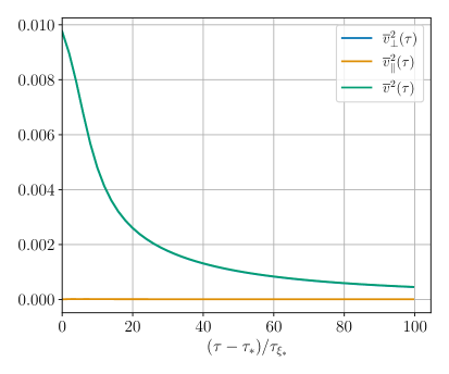
Figure 27: Evolution of the kinetic energy $\overline{v}^{2}$, decomposed into the vortical, $\overline{v}_{\perp}^{2}$, and longitudinal, $\overline{v}_{\parallel}^{2}$, components (see Eq. F.2). The central panel shows simulation (A).

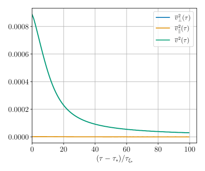
(a) Simulation (B).

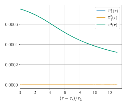
(b) Simulation (C).

Figure 28: Evolution of the kinetic energy $\overline{v}^{2}$, decomposed into the vortical, $\overline{v}_{\perp}^{2}$, and longitudinal, $\overline{v}_{\parallel}^{2}$, components (see Eq. F.2). The left and right panels show simulation (B) and (C) respectively.

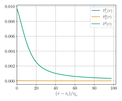
(a) Simulation (D).

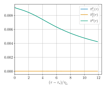
(b) Simulation (E).

Figure 29: Evolution of the kinetic energy $\overline{v}^{2}$, decomposed into the vortical, $\overline{v}_{\perp}^{2}$, and longitudinal, $\overline{v}_{\parallel}^{2}$, components (see Eq. F.2). The left and right panels show simulation (D) and (E) respectively.

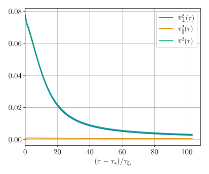
(a) Simulation (F).

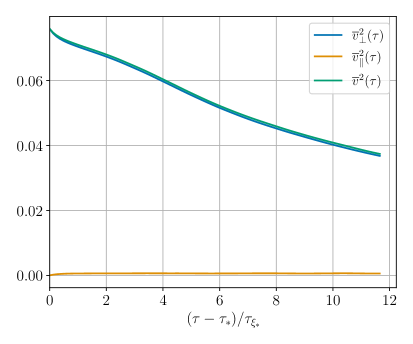
(b) Simulation (G).

Figure 30: Evolution of the kinetic energy $\overline{v}^{2}$, decomposed into the vortical, $\overline{v}_{\perp}^{2}$, and longitudinal, $\overline{v}_{\parallel}^{2}$, components (see Eq. F.2). The left and right panels show simulation (F) and (G) respectively.

References

- [1] E. Witten, Cosmic Separation of Phases, Phys. Rev. D 30 (1984) 272.
- [2] C. Hogan, Gravitational radiation from cosmological phase transitions, MNRAS 218 (1986) 629.
- [3] M.S. Turner and F. Wilczek, Relic gravitational waves and extended inflation, Phys. Rev. Lett. 65 (1990) 3080.
- [4] A. Kosowsky, M.S. Turner and R. Watkins, Gravitational radiation from colliding vacuum bubbles, Phys. Rev. D 45 (1992) 4514.
- [5] A. Kosowsky and M.S. Turner, Gravitational radiation from colliding vacuum bubbles: envelope approximation to many bubble collisions, Phys. Rev. D 47 (1993) 4372 [astro-ph/9211004].
- [6] M. Kamionkowski, A. Kosowsky and M.S. Turner, Gravitational radiation from first order phase transitions, Phys. Rev. D49 (1994) 2837 [astro-ph/9310044].
- [7] K. Kajantie, M. Laine, K. Rummukainen and M.E. Shaposhnikov, Is there a hot electroweak phase transition at m(H) larger or equal to m(W)?, Phys. Rev. Lett. 77 (1996) 2887 [hep-ph/9605288].
- [8] C. Caprini et al., Detecting gravitational waves from cosmological phase transitions with LISA: an update, JCAP 03 (2020) 024 [1910.13125].
- [9] LISA collaboration, Laser interferometer space antenna, 1702.00786.
- [10] C. Caprini et al., Science with the space-based interferometer eLISA. II: Gravitational waves from cosmological phase transitions, JCAP 1604 (2016) 001 [1512.06239].
- [11] R. Caldwell et al., Detection of Early-Universe Gravitational Wave Signatures and Fundamental Physics, 2203.07972.
- [12] S.J. Huber and T. Konstandin, Gravitational wave production by collisions: More bubbles, JCAP 0809 (2008) 022 [0806.1828].
- [13] D.J. Weir, Revisiting the envelope approximation: gravitational waves from bubble collisions, Phys. Rev. D 93 (2016) 124037 [1604.08429].
- [14] T. Konstandin, Gravitational radiation from a bulk flow model, JCAP 03 (2018) 047 [1712.06869].
- [15] D. Cutting, M. Hindmarsh and D.J. Weir, Gravitational waves from vacuum first-order phase transitions: From the envelope to the lattice, Phys. Rev. D97 (2018) 123513 [1802.05712].
- [16] D. Cutting, E.G. Escartin, M. Hindmarsh and D.J. Weir, Gravitational waves from vacuum first order phase transitions II: from thin to thick walls, Phys. Rev. D 103 (2021) 023531 [2005.13537].
- [17] M. Lewicki and V. Vaskonen, Gravitational wave spectra from strongly supercooled phase transitions, Eur. Phys. J. C 80 (2020) 1003 [2007.04967].
- [18] M. Lewicki and V. Vaskonen, Gravitational waves from colliding vacuum bubbles in gauge theories, Eur. Phys. J. C 81 (2021) 437 [2012.07826].
- [19] O. Gould, S. Sukuvaara and D. Weir, Vacuum bubble collisions: From microphysics to gravitational waves, Phys. Rev. D 104 (2021) 075039 [2107.05657].
- [20] C. Caprini, R. Durrer and G. Servant, Gravitational wave generation from bubble collisions in first-order phase transitions: An analytic approach, Phys. Rev. D77 (2008) 124015 [0711.2593].
- [21] R. Jinno and M. Takimoto, Gravitational waves from bubble collisions: An analytic derivation, Phys. Rev. D 95 (2017) 024009 [1605.01403].
- [22] R. Jinno and M. Takimoto, Gravitational waves from bubble dynamics: Beyond the Envelope, JCAP 01 (2019) 060 [1707.03111].
- [23] M. Hindmarsh, S.J. Huber, K. Rummukainen and D.J. Weir, Gravitational waves from the sound of a first order phase transition, Phys. Rev. Lett. 112 (2014) 041301 [1304.2433].
- [24] M. Hindmarsh, S.J. Huber, K. Rummukainen and D.J. Weir, Numerical simulations of acoustically generated gravitational waves at a first order phase transition, Phys. Rev. D92 (2015) 123009 [1504.03291].
- [25] M. Hindmarsh, S.J. Huber, K. Rummukainen and D.J. Weir, Shape of the acoustic gravitational wave power spectrum from a first order phase transition, Phys. Rev. D96 (2017) 103520 [1704.05871].
- [26] M. Hindmarsh, Sound shell model for acoustic gravitational wave production at a first-order phase transition in the early Universe, Phys. Rev. Lett. 120 (2018) 071301 [1608.04735].
- [27] M. Hindmarsh and M. Hijazi, Gravitational waves from first order cosmological phase transitions in the Sound Shell Model, JCAP 12 (2019) 062 [1909.10040].
- [28] R. Jinno, T. Konstandin and H. Rubira, A hybrid simulation of gravitational wave production in first-order phase transitions, JCAP 04 (2021) 014 [2010.00971].
- [29] U.-L. Pen and N. Turok, Shocks in the Early Universe, Phys. Rev. Lett. 117 (2016) 131301 [1510.02985].
- [30] J. Dahl, M. Hindmarsh, K. Rummukainen and D. Weir, Decay of acoustic turbulence in two dimensions and implications for cosmological gravitational waves, 2112.12013.
- [31] D. Cutting, M. Hindmarsh and D.J. Weir, Vorticity, kinetic energy, and suppressed gravitational wave production in strong first order phase transitions, 1906.00480.
- [32] C. Caprini and R. Durrer, Gravitational waves from stochastic relativistic sources: Primordial turbulence and magnetic fields, Phys. Rev. D 74 (2006) 063521 [astro-ph/0603476].
- [33] G. Gogoberidze, T. Kahniashvili and A. Kosowsky, The Spectrum of Gravitational Radiation from Primordial Turbulence, Phys. Rev. D 76 (2007) 083002 [0705.1733].
- [34] T. Kahniashvili, L. Campanelli, G. Gogoberidze, Y. Maravin and B. Ratra, Gravitational Radiation from Primordial Helical Inverse Cascade MHD Turbulence, Phys. Rev. D 78 (2008) 123006 [0809.1899].
- [35] T. Kahniashvili, G. Gogoberidze and B. Ratra, Gravitational Radiation from Primordial Helical MHD Turbulence, Phys. Rev. Lett. 100 (2008) 231301 [0802.3524].
- [36] C. Caprini, R. Durrer and G. Servant, The stochastic gravitational wave background from turbulence and magnetic fields generated by a first-order phase transition, JCAP 12 (2009) 024 [0909.0622].
- [37] C. Caprini, R. Durrer and E. Fenu, Can the observed large scale magnetic fields be seeded by helical primordial fields?, JCAP 11 (2009) 001 [0906.4976].
- [38] P. Niksa, M. Schlederer and G. Sigl, Gravitational Waves produced by Compressible MHD Turbulence from Cosmological Phase Transitions, Class. Quant. Grav. 35 (2018) 144001 [1803.02271].
- [39] Y. Kaneda, Lagrangian and Eulerian time correlations in turbulence, Physics of Fluids A: Fluid Dynamics 5 (1993) 2835.
- [40] R.H. Kraichnan, Kolmogorov’s hypotheses and eulerian turbulence theory, The Physics of Fluids 7 (1964) 1723 [https://aip.scitation.org/doi/pdf/10.1063/1.2746572].
- [41] A. Roper Pol, A. Brandenburg, T. Kahniashvili, A. Kosowsky and S. Mandal, The timestep constraint in solving the gravitational wave equations sourced by hydromagnetic turbulence, Geophys. Astrophys. Fluid Dynamics 114 (2020) 130 [1807.05479].
- [42] A. Roper Pol, S. Mandal, A. Brandenburg, T. Kahniashvili and A. Kosowsky, Numerical simulations of gravitational waves from early-universe turbulence, Phys. Rev. D 102 (2020) 083512 [1903.08585].
- [43] T. Kahniashvili, A. Brandenburg, G. Gogoberidze, S. Mandal and A. Roper Pol, Circular polarization of gravitational waves from early-Universe helical turbulence, Phys. Rev. Res. 3 (2021) 013193 [2011.05556].
- [44] A. Brandenburg, G. Gogoberidze, T. Kahniashvili, S. Mandal, A. Roper Pol and N. Shenoy, The scalar, vector, and tensor modes in gravitational wave turbulence simulations, 2103.01140.
- [45] G.-W. He, M. Wang and S.K. Lele, On the computation of space-time correlations by large-eddy simulation, Physics of Fluids 16 (2004) 3859 [https://doi.org/10.1063/1.1779251].
- [46] A. Roper Pol, C. Caprini, A. Neronov and D. Semikoz, The gravitational wave signal from primordial magnetic fields in the Pulsar Timing Array frequency band, 2201.05630.
- [47] C. Caprini and D.G. Figueroa, Cosmological backgrounds of gravitational waves, Class. Quant. Grav. 35 (2018) 163001 [1801.04268].
- [48] P.A. Davidson, Turbulence: An Introduction for Scientists and Engineers, Oxford University Press, Oxford, UK ; New York (2004).
- [49] A. Kolmogorov, The Local Structure of Turbulence in Incompressible Viscous Fluid for Very Large Reynolds’ Numbers, Akademiia Nauk SSSR Doklady 30 (1941) 301.
- [50] T. von Karman, Progress in the Statistical Theory of Turbulence, Proceedings of the National Academy of Sciences 34 (1948) 530.
- [51] A. Brandenburg, T. Kahniashvili, S. Mandal, A. Roper Pol, A.G. Tevzadze and T. Vachaspati, Evolution of hydromagnetic turbulence from the electroweak phase transition, Phys. Rev. D 96 (2017) 123528 [1711.03804].
- [52] W.K. George, The decay of homogeneous isotropic turbulence, Physics of Fluids A 4 (1992) 1492.
- [53] A. Brandenburg, T. Kahniashvili and A.G. Tevzadze, Nonhelical inverse transfer of a decaying turbulent magnetic field, Phys. Rev. Lett. 114 (2015) 075001 [1404.2238].
- [54] J. Reppin and R. Banerjee, Nonhelical turbulence and the inverse transfer of energy: A parameter study, Phys. Rev. E 96 (2017) 053105 [1708.07717].
- [55] M. Christensson, M. Hindmarsh and A. Brandenburg, Inverse cascade in decaying 3-D magnetohydrodynamic turbulence, Phys. Rev. E 64 (2001) 056405 [astro-ph/0011321].
- [56] L. Campanelli, On the self-similarity of nonhelical magnetohydrodynamic turbulence, Eur. Phys. J. C 76 (2016) 504 [1511.06797].
- [57] P. Olesen, Inverse transfer of self-similar decaying turbulent non-helical magnetic field, 1509.08962.
- [58] A. Brandenburg and T. Kahniashvili, Classes of hydrodynamic and magnetohydrodynamic turbulent decay, Phys. Rev. Lett. 118 (2017) 055102 [1607.01360].
- [59] P. Olesen, On inverse cascades in astrophysics, Phys. Lett. B 398 (1997) 321 [astro-ph/9610154].
- [60] P.D. Ditlevsen, M.H. Jensen and P. Olesen, Scaling in decaying hydrodynamic turbulence, Physica A 342 (2004) 471 [nlin/0205055].
- [61] L. Campanelli, Evolution of Magnetic Fields in Freely Decaying Magnetohydrodynamic Turbulence, Phys. Rev. Lett. 98 (2007) 251302 [0705.2308].
- [62] L. Landau and E. Lifshitz, Fluid Mechanics: Volume 6, no. v. 6, Elsevier Science (2013).
- [63] T. Teitelbaum and P.D. Mininni, Large-scale effects on the decay of rotating helical and non-helical turbulence, Physica Scripta Volume T 142 (2010) 014003 [0911.0356].
- [64] S.J. Camargo and S.J. Tasso, Renormalization group in magnetohydrodynamic turbulence, Physics of Fluids B: Plasma Physics 4 (1992) 1199.
- [65] T. Shiromizu, Inverse cascade of primordial magnetic field in MHD turbulence, Phys. Lett. B 443 (1998) 127 [astro-ph/9810339].
- [66] V. Mons, J.-C. Chassaing, T. Gomez and P. Sagaut, Is isotropic turbulence decay governed by asymptotic behavior of large scales? an eddy-damped quasi-normal markovian-based data assimilation study, Physics of Fluids 26 (2014) 115105 [https://doi.org/10.1063/1.4901448].
- [67] P. Schaefer, M. Gampert, J. Goebbert, M. Gauding and N. Peters, Asymptotic analysis of homogeneous isotropic decaying turbulence with unknown initial conditions, Journal of Turbulence 12 (2011) 1.
- [68] M. Meldi and P. Sagaut, On non-self-similar regimes in homogeneous isotropic turbulence decay, Journal of Fluid Mechanics 711 (2012) 364.
- [69] Y. Zhou, Turbulence theories and statistical closure approaches, Phys. Rept. 935 (2021) 1.
- [70] T. Sanada and V. Shanmugasundaram, Random sweeping effect in isotropic numerical turbulence, Physics of Fluids A: Fluid Dynamics 4 (1992) 1245.
- [71] A. Gorbunova, G. Balarac, L. Canet, G. Eyink and V. Rossetto, Spatio-temporal correlations in three-dimensional homogeneous and isotropic turbulence, Phys. Fluids 33 (2021) 045114.
- [72] Y.-H. Dong and P. Sagaut, A study of time correlations in lattice Boltzmann-based large-eddy simulation of isotropic turbulence, Physics of Fluids 20 (2008) 035105.
- [73] M. Wilczek and Y. Narita, Wave-number–frequency spectrum for turbulence from a random sweeping hypothesis with mean flow, Phys. Rev. E 86 (2012) 066308.
- [74] Y. Kaneda and T. Gotoh, Lagrangian velocity autocorrelation in isotropic turbulence, Physics of Fluids A: Fluid Dynamics 3 (1991) 1924.
- [75] M.G. Genton, Classes of kernels for machine learning: A statistics perspective, J. Mach. Learn. Res. 2 (2002) 299–312.
- [76] J. Mercer, Functions of Positive and Negative Type, and their Connection with the Theory of Integral Equations, Philosophical Transactions of the Royal Society of London Series A 209 (1909) 415.
- [77] C. Caprini, R. Durrer, T. Konstandin and G. Servant, General Properties of the Gravitational Wave Spectrum from Phase Transitions, Phys. Rev. D 79 (2009) 083519 [0901.1661].
- [78] R. Silverman, Locally stationary random processes, IRE Transactions on Information Theory 3 (1957) 182.
- [79] D. Higdon, J. Swall and J. Kern, Non-stationary spatial modeling, Bayesian statistics 6 (1999) 761.
- [80] K. Enqvist, J. Ignatius, K. Kajantie and K. Rummukainen, Nucleation and bubble growth in a first order cosmological electroweak phase transition, Phys.Rev. D45 (1992) 3415.
- [81] A. Brandenburg, K. Enqvist and P. Olesen, Large scale magnetic fields from hydromagnetic turbulence in the very early universe, Phys. Rev. D 54 (1996) 1291 [astro-ph/9602031].
- [82] J. Wilson and G. Matthews, Relativistic Numerical Hydrodyamics, Cambridge University Press, Cambridge (2003).
- [83] B. Van Leer, Towards the ultimate conservative difference scheme. iv. a new approach to numerical convection, Journal of Computational Physics 23 (1977) 276.
- [84] P. Anninos and P.C. Fragile, Non-oscillatory central difference and artificial viscosity schemes for relativistic hydrodynamics, Astrophys. J. Suppl. 144 (2003) 243 [astro-ph/0206265].
- [85] J. Garcia-Bellido, D.G. Figueroa and A. Sastre, A Gravitational Wave Background from Reheating after Hybrid Inflation, Phys. Rev. D 77 (2008) 043517 [0707.0839].
- [86] M.B. Hindmarsh, M. Lüben, J. Lumma and M. Pauly, Phase transitions in the early universe, SciPost Phys. Lect. Notes 24 (2021) 1 [2008.09136].
- [87] H.-K. Guo, K. Sinha, D. Vagie and G. White, Phase Transitions in an Expanding Universe: Stochastic Gravitational Waves in Standard and Non-Standard Histories, JCAP 01 (2021) 001 [2007.08537].
- [88] J. Ellis, M. Lewicki and J.M. No, Gravitational waves from first-order cosmological phase transitions: lifetime of the sound wave source, JCAP 07 (2020) 050 [2003.07360].
- [89] G.P. Lepage, A new algorithm for adaptive multidimensional integration, Journal of Computational Physics 27 (1978) 192.
- [90] G.P. Lepage, Adaptive multidimensional integration: VEGAS enhanced, J. Comput. Phys. 439 (2021) 110386 [2009.05112].
- [91] A. Brandenburg and S. Boldyrev, The turbulent stress spectrum in the inertial and subinertial ranges, Astrophys. J. 892 (2020) 80 [1912.07499].
- [92] A. Brandenburg, Y. He, T. Kahniashvili, M. Rheinhardt and J. Schober, Relic gravitational waves from the chiral magnetic effect, Astrophys. J. 911 (2021) 110 [2101.08178].
- [93] A. Roper Pol, S. Mandal, A. Brandenburg and T. Kahniashvili, Polarization of gravitational waves from helical MHD turbulent sources, JCAP 04 (2022) 019 [2107.05356].