Moment-based Invariants for Probabilistic Loops with Non-polynomial Assignments

Abstract

We present a method to automatically approximate moment-based invariants of probabilistic programs with non-polynomial updates of continuous state variables to accommodate more complex dynamics. Our approach leverages polynomial chaos expansion to approximate non-linear functional updates as sums of orthogonal polynomials. We exploit this result to automatically estimate state-variable moments of all orders in Prob-solvable loops with non-polynomial updates. We showcase the accuracy of our estimation approach in several examples, such as the turning vehicle model and the Taylor rule in monetary policy.

1 Introduction

Probabilistic programs (PPs) are becoming widely employed in many areas including AI applications, security/privacy protocols or modeling stochastic dynamical systems. The study of the properties of these processes requires knowledge of their distribution; that is, the distribution(s) of the random variable(s) generated by executing the probabilistic program.

The characterization of many distributions can be accomplished via their moments. In [2] the authors introduced a class of probabilistic programs, Prob-solvable loops, for which moment-based invariants over the state variables of the programs are automatically computed as a closed-form expression. A Prob-solvable loop consists of an initialization section and a non-nested loop where the variables can be updated by drawing from distributions determined by their moments (e.g., Bernoulli, Normal) and using polynomial arithmetic. However, modeling complex dynamics often requires the use of non-polynomial updates, such as in the turning vehicle example in Fig. 1. An open research question is how to leverage the class of Prob-solvable loops to estimate moment-based invariants as closed-form expressions for probabilistic loops with updates governed by non-polynomial non-linear functions.

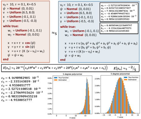
Figure 1: On the top left a probabilistic loop modeling the behaviour of a turning vehicle [25] using non-polynomial (cos, sin) updates in the loop body. On top right a Prob-Solvable loop obtained by approximating the cos, sin functions using polynomial chaos expansion (up to 5th degree). In the middle the expected position $(x,y)$ computed automatically from the Prob-Solvable loop as a closed-form expression in the number of the loop iterations $n$. In the bottom center and right the comparison among the true and the estimated distribution for a fixed iteration (we execute the loop for $n=20$ iterations and $8\cdot 10^{5}$ repetitions).

At the heart of our approach is the decomposition of a random function into a linear combination of basis functions that are orthogonal polynomials. We accommodate non-polynomial updates of program variables to allow for more complicated dynamics. By expressing the non-linear functionals of the updates as sums of orthogonal polynomials, we can apply the approach in [2, 3] to automatically estimate the moments of all the program random variables. Our approach is within the framework of general polynomial chaos expansion (gPCE) [34]. As such, it converges to the truth with guaranteed recovery of the moments of random variables with complex distributions. We focus on state variables with continuous distributions with updates that are square-integrable functionals and use general polynomial chaos expansion to represent them. In Fig. 1 we illustrate our approach via the turning vehicle example, where we estimate the expected position of a vehicle. In this example, we approximate the original cosine and sine functions with 5$th$ degree polynomials and obtain a Prob-solvable loop. This enables the automatic computation of the moments in closed-form at each loop iteration ($n$) using the approach proposed in [2].

Related Work.

[25] proposed polynomial forms to represent distributions of state variables. Polynomial forms are generalizations of affine forms [4] and use the Taylor series expansion to represent functions of random variables generated in a PP. Functions can be only approximated in a small interval around a fixed point, otherwise high order derivatives are required to guarantee sufficient accuracy of the approximation. As a consequence, functions with unbounded support cannot be handled with this approach.

So-called Taylor models have been proposed in [19, 23, 5] for reachability analysis of (non-probabilistic) non-linear dynamical systems. Taylor models combine polynomials and error intervals to capture the set of reachable states after some fixed time horizon. Application of Taylor series expansions for generalized functions of probabilistic distributions can also be found in [27, 31].

[17] introduced trigonometric and mixed-trigonometric-polynomial moments to obtain an exact description of the moments of uncertain states for nonlinear autonomous and robotic systems over the planning horizon. This approach can only handle systems encoded in PPs, where all nonlinear transformations take standard, trigonometric, or mixed-trigonometric polynomial forms.

Polynomial chaos expansion based methods have been extensively used for uncertainty quantification in engineering problems of solid and fluid mechanics (e.g. [13, 9, 16]), computational fluid dynamics (e.g., [18]), flow through porous media [11, 12], thermal problems [15], analysis of turbulent velocity fields [6, 20], differential equations (e.g., [32, 34]), and, more recently, geosciences and meteorology (e.g., [10, 14, 7]).

Outline.

Sec. 2 reviews the notion of Prob-solvable Loop and the general theory of Polynomial Chaos Expansion (PCE). Sec. 3 presents our PCE algorithm and the conditions under which it produces accurate approximations to general random functions in probabilistic program loops. Sec. 4 combines general PCE with Prob-solvable loops to automatically compute moments of all orders of state variables. There, we also characterize the structure a probabilistic program ought to have in order to be compatible with the Prob-solvable loops approach for computation of moments. Sec. 5 demonstrates the accuracy and feasibility of our approach on different benchmarks as compared with the state-of-the-art. We conclude in Sec. 6.

2 Preliminaries

2.1 Prob-Solvable Loops

[2] defined the class of Prob-solvable loops for which moments of all orders of program variables can be computed symbolically: given a Prob-solvable loop and a program variable $x$, their method computes a closed-form solution for $\mathbb{E}(x_{n}^{k})$ for arbitrary $k\in{\mathbb{N}}$, where $n$ denotes the $n$th loop iteration. Prob-solvable loops are restricted to polynomial variable updates.

Definition 1 (Prob-solvable loops)

Let $m\in{\mathbb{N}}$ and $x_{1},\ldots x_{m}$ denote real-valued program variables. A Prob-solvable loop with program variables $x_{1},\ldots x_{m}$ is a loop of the form

$$I;\texttt{while(true)}\{U\},$$

where

• $I$ is a sequence of initial assignments over a subset of $\{x_{1},\ldots,x_{m}\}$. The initial values of $x_{i}$ can be drawn from a known distribution. They can also be real constants.

• $U$ is the loop body and is a sequence of $m$ random updates, each of the form:

  $$x_{i}=\textit{Dist}\quad\text{or}\quad x_{i}:=ax_{i}+P_{i}(x_{1},\dots x_{i-1})$$

  where $a\in$, $P_{i}\in[x_{1},\ldots,x_{i-1}]$ is a polynomial over program variables $x_{1},\ldots,x_{i-1}$ and Dist is a distribution independent from program variables with computable moments.

Many real-life systems exhibit non-polynomial dynamics and require more general updates, such as, for example, trigonometric or exponential functions. In this work, we develop a method that allows approximation of non-polynomial assignments in probabilistic loops by polynomial assignments. In doing so, we can use the methods for Prob-solvable loops to compute the moments for a broader class of stochastic systems.

The programming model we use (Definition 1) is a simplified version of the Prob-solvable model as introduced in [2]. Our approach, described in the following sections, is not limited to this simple fragment of the Prob-solvable and can be used for Prob-solvable loops as originally defined as well as other more general probabilistic loops. The only requirement is that the loops satisfy the conditions in Section 3.1.

2.2 Polynomial Chaos Expansion

Polynomial chaos expansion recovers a random variable in terms of a linear combination of functionals whose entries are known random variables, sometimes called germs, or, basic variables. Let $(\Omega,\Sigma,\mathbb{P})$ be a probability space, where $\Omega$ is the set of elementary events, $\Sigma$ is a $\sigma$-algebra of subsets of $\Omega$, and $\mathbb{P}$ is a probability measure on $\Sigma$. Suppose $X$ is a real-valued random variable defined on $(\Omega,\Sigma,\mathbb{P})$, such that

$$\mathbb{E}(X^{2}) =\int_{\Omega}X^{2}(\omega)d\mathbb{P}(\omega)<\infty.$$ (1)

The space of all random variables $X$ satisfying (1) is denoted by $L^{2}(\Omega,\Sigma,\mathbb{P})$. That is, the elements of $L^{2}(\Omega,\Sigma,\mathbb{P})$ are real-valued random variables defined on $(\Omega,\Sigma,\mathbb{P})$ with finite second moments. If we define the inner product as

$$\mathbb{E}(XY) =(X,Y)=\int_{\Omega}X(\omega)Y(\omega)d\mathbb{P}(\omega)$$ (2)

and norm $||X||=\sqrt{\mathbb{E}(X^{2})}=\sqrt{\int_{\Omega}X^{2}(\omega)d\mathbb{P}(\omega)}$, then $L^{2}(\Omega,\Sigma,\mathbb{P})$ is a Hilbert space; i.e., an infinite dimensional linear space of functions endowed with an inner product and a distance metric. Elements of a Hilbert space can be uniquely specified by their coordinates with respect to an orthonormal basis of functions, in analogy with Cartesian coordinates in the plane. Convergence with respect to $||\cdot||$ is called mean-square convergence. A particularly important feature of a Hilbert space is that when the limit of a sequence of functions exists, it belongs to the space.

The elements in $L^{2}(\Omega,\Sigma,\mathbb{P})$ can be classified in two groups: basic and generic random variables, which we want to decompose using the elements of the first set of basic variables. [8] showed that the basic random variables that can be used in the decomposition of other functions have finite moments of all orders with continuous probability density functions (pdf).

The $\sigma$-algebra generated by the basic random variable $Z$ is denoted by $\sigma(Z)$. Suppose we restrict our attention to decompositions of a random variable $X=g(Z)$, where $g$ is a function with $g(Z)\in L^{2}(\Omega,\sigma(Z),\mathbb{P})$ and the basic random variable $Z$ determines the class of orthogonal polynomials $\{\phi_{i}(Z),i\in\mathbb{N}\}$,

$$\left<\phi_{i}(Z),\phi_{j}(Z)\right> =\int_{\Omega}\phi_{i}(Z(\omega))\phi_{j}(Z(\omega))d\mathbb{P}(\omega)$$

$$=\int\phi_{i}(x)\phi_{j}(x)f_{Z}(x)dx=\begin{cases}1&i=j\\ 0&i\neq j\end{cases}$$ (3)

which is a polynomial chaos basis. If $Z$ is normal with mean zero, the Hilbert space $L^{2}(\Omega,\sigma(Z),\mathbb{P})$ is called Gaussian and the related set of polynomials is represented by the family of Hermite polynomials (see, for example, [34]) defined on the whole real line. Hermite polynomials form a basis of $L^{2}(\Omega,\sigma(Z),\mathbb{P})$. Therefore, every random variable $X$ with finite second moment can be approximated by the truncated PCE

$$X^{(d)} =\sum_{i=0}^{d}c_{i}\phi_{i}(Z),$$ (4)

for suitable coefficients $c_{i}$ that depend on the random variable $X$. The truncation parameter $d$ is the highest polynomial degree in the expansion. Since the polynomials are orthogonal,

$$c_{i} =\frac{1}{||\phi_{i}||^{2}}\left<X,\phi_{i}\right>=\frac{1}{||\phi_{i}||^{2}}\left<g,\phi_{i}\right>=\frac{1}{||\phi_{i}||^{2}}\int g(x)\phi_{i}(x)f_{Z}(x)dx.$$ (5)

The truncated PCE of $X$ in (4) converges in mean square to $X$ [8, Sec. 3.1]. The first two moments of (4) are determined by

$$\mathbb{E}(X^{(d)}) =c_{0},$$ (6)

$$\mathbb{V}\mathrm{ar}(X^{(d)}) =\sum_{i=1}^{d}c_{i}^{2}||\phi_{i}||^{2}.$$ (7)

Representing a random variable by a series of Hermite polynomials in a countable sequence of independent Gaussian random variables is known as Wiener–Hermite polynomial chaos expansion. In applications of Wiener–Hermite PCEs, the underlying Gaussian Hilbert space is often taken to be the space spanned by a sequence $\{Z_{i},i\in\mathbb{N}\}$ of independent standard Gaussian basic random variables, $Z_{i}\sim\mathcal{N}(0,1)$. For computational purposes, the countable sequence $\{Z_{i},i\in\mathbb{N}\}$ is restricted to a finite number $k\in\mathbb{N}$ of random variables. The Wiener–Hermite polynomial chaos expansion converges for random variables with finite second moment. Specifically, for any random variable $X\in L^{2}(\Omega,\sigma(\{Z_{i},i\in\mathbb{N}\}),\mathbb{P})$, the approximation (4) satisfies

$$X_{k}^{(d)} \to X\quad\mbox{as }d,k\to\infty$$ (8)

in mean-square convergence. The distribution of $X$ can be quite general; e.g., discrete, singularly continuous, absolutely continuous as well as of mixed type.

3 Polynomial Chaos Expansion Algorithm

3.1 Random Function Representation

In this section, we state the conditions under which the estimated polynomial is an unbiased and consistent estimator and has exponential convergence rate.
Suppose $k$ continuous random variables $Z_{1},\ldots,Z_{k}$ are used to introduce stochasticity in a PP, with corresponding cumulative distribution functions (cdf) $F_{Z_{i}}$ for $i=1,\ldots,k$. Also, suppose all $k$ distributions have probability density functions, and let ${\mathbf{Z}}=(Z_{1},\ldots,Z_{k})$ with cdf $F_{{\mathbf{Z}}}$. We assume that the elements of ${\mathbf{Z}}$ satisfy the following conditions:

• $Z_{i},i=1,\ldots,k$, are independent.

• We consider functions $g$ such that $g({\mathbf{Z}})\in L^{2}(\mathcal{Q},F_{\mathbf{Z}})$, where $\mathcal{Q}$ is the support of the joint distribution of ${\mathbf{Z}}=(Z_{1},\ldots,Z_{k})$ .

• All random variables $Z_{i}$ have distributions that are uniquely defined by their moments.

Under condition (A), the joint cdf of the components of ${\mathbf{Z}}$ is $F_{{\mathbf{Z}}}=\prod_{i=1}^{k}F_{Z_{i}}$. To ensure the construction of unbiased estimators with optimal exponential convergence rate (see [34], [8]) in the context of probabilistic loops, we further introduce the following assumptions:

• $g$ is a function of a fixed number of basic variables (arguments) over all loop iterations.

• If ${\mathbf{Z}}(j)=(Z_{1}(j),\ldots,Z_{k}(j))$ is the stochastic argument of $g$ at iteration $j$, then $F_{Z_{i}(j)}(x)=F_{Z_{i}(l)}(x)$ for all pairs of iterations $(j,l)$ and $x$ in the support of $F_{Z_{i}}$.

If Conditions (D) and (E) are not met, then the polynomial coefficients in the PCE need be computed for each loop iteration individually to ensure optimal convergence rate. It is straightforward to show the following proposition.

Proposition 1

If functions $f$ and $g$ satisfy conditions (B) and (D), and ${\mathbf{Z}}=(Z_{1},\ldots,Z_{k_{1}})$, ${\mathbf{Y}}=(Y_{1},\ldots,Y_{k_{2}})$ satisfy conditions (A), (C) and (E) and are mutually independent, then their sum, $f({\mathbf{Z}})+g({\mathbf{Y}})$, and product, $f({\mathbf{Z}})\cdot g({\mathbf{Y}})$, also satisfy conditions (B) and (D).

Figure 2: Illustration of PCE algorithm

3.2 PCE Algorithm

Let $Z_{1},\ldots,Z_{k}$ be independent continuous random variables, with respective cdfs $F_{i}$, satisfying conditions (A), (B) and (C), and ${\mathbf{Z}}=(Z_{1},\ldots,Z_{k})^{T}$ with cdf ${\mathbf{F}}=\prod_{i=1}^{k}F_{i}$ and support $\mathcal{Q}$. The function $g:^{k}\to$, with $g\in L^{2}(\mathcal{Q},{\mathbf{F}})$ can be approximated with the truncated orthogonal polynomial expansion, as described in Fig. 2,

$$g({\mathbf{Z}}) \approx\hat{g}({\mathbf{Z}})=\sum_{\begin{subarray}{c}d_{i}\in\{0,\ldots,\bar{d}_{i}\},\\ i=1,\ldots,k\end{subarray}}c(d_{1},\ldots,d_{k})z_{1}^{d_{1}}\cdots z_{k}^{d_{k}}=\sum_{j=1}^{L}c_{j}\prod\limits_{i=1}^{k}\bar{p}_{i}^{d_{ji}}(z_{i}),$$ (9)

where

• $\bar{p}_{i}^{d_{ji}}(z_{i})$ is a polynomial of degree $d_{ji}$, and belongs to the set of orthogonal polynomials with respect to $F_{Z_{i}}$ that are calculated with the Gram-Schmidt orthogonalization procedure;

• $\bar{d}_{i}=\max\limits_{j}(d_{ji})$ is the highest degree of the univariate orthogonal polynomial, for $i=1,\ldots,k$;

• $L=\prod\limits_{i=1}^{k}(1+\bar{d}_{i})$ is the total number of multivariate orthogonal polynomials and equals the truncation constant;

• $c_{j}$ are the Fourier coefficients.

The Fourier coefficients are calculated using

$$c_{j} =\int\limits_{\mathcal{Q}}g(z_{1},...,z_{k})p_{i}^{d_{ji}}(z_{i})d{\mathbf{F}}=\idotsint\limits_{\mathcal{Q}}g(z_{1},...,z_{k})\prod\limits_{i=1}^{k}\bar{p}_{i}^{d_{ji}}(z_{i})dF_{Z_{k}}...dF_{Z_{1}},$$ (10)

by Fubini’s theorem. An example with calculation details of the coefficients in (10) is given in Appendix 0.B.

Example 1

Returning to the Turning Vehicle model in Fig. 1, the non-polynomial functions to approximate are $g_{1}=cos$ and $g_{2}=sin$ from the updates of program variables $y,x$, respectively. In both cases, we only need to consider a single basic random variable, $Z\sim\mathcal{N}(0,0.01)$ ($\psi$ in Fig. 1).

For the approximation, we use polynomials of degree up to $5$. Eqn. (9) has the following form for the two functions,

$$\hat{g}_{1}(z)=cos(\psi)=a_{0}+a_{1}\psi+...+a_{5}\psi^{5}$$ (11)

and

$$\hat{g}_{2}(z)=sin(\psi)=b_{0}+b_{1}\psi+...+b_{5}\psi^{5}.$$ (12)

We compute the coefficients $a_{i},b_{i}$ in equations (11)-(12) using (10) to obtain the values shown in Fig. 1.

Complexity.

Assuming the expansion is carried out up to the same polynomial degree $d$ for each basic variable, $\bar{d}_{i}=d$, $\forall i=1,...,k$. This implies $d=\sqrt[k]{L}-1$. The complexity of the scheme is $\mathcal{O}(sd^{2}k+s^{k}d^{k})$, where $\mathcal{O}(s)$ is the complexity of computing univariate integrals.

The complexity of our approximation scheme is comprised of two parts: (1) the orthogonalization process and (2) the calculation of coefficients. Regarding (1), we orthogonalize and normalize $k$ sets of $d$ basic linearly independent polynomials during the Gram-Schmidt process. For degree $d{=}1$, we need to calculate one integral, the inner product with the previous polynomial. Additionally, we need to compute one more integral, the norm of itself (for normalization). For each subsequent degree $d^{\prime}$, we must calculate $d^{\prime}$ additional new integrals. The computation of each integral has complexity $\mathcal{O}(s)$. Regarding (2), the computation of the coefficients requires calculating $L{=}(d{+}1)^{k}$ integrals with $k$-variate functions as integrands.

We define the approximation error to be

$$se(\hat{g})=\sqrt{\int\limits_{\mathcal{Q}}\left(g(z_{1},...,z_{k})-\hat{g}(z_{1},...,z_{k})\right)^{2}dF_{Z_{1}}\ldots dF_{Z_{k}}}$$ (13)

since $\mathbb{E}(\hat{g}(Z_{1},...,Z_{k}))=g(Z_{1},\cdots,Z_{k})$ by construction.

Appendix 0.C contains examples of polynomial chaos expansion for functions of up to three variables. The implementation of this algorithm may become challenging when the random functions have complicated forms and the number of parametric uncertainties is large. In this case, the calculation of the PCE coefficients involves high dimensional integration, which may prove difficult and time prohibitive for real-time applications [26].

4 Prob-Solvable Loops for General Non-Polynomial Functions

PCE allows incorporating non-polynomial updates into Prob-solvable loop programs and use the algorithm in [2] and exact tools, such as Polar [21], for moment (invariant) computation. We identify two classes of programs based on how the distributions of the random variables generated by the programs vary.

4.1 Iteration-Stable Distributions of Random Arguments

Let $\mathcal{P}$ be an arbitrary Prob-solvable loop and suppose that a (non-basic) state variable $x\in\mathcal{P}$ has a non-polynomial $L^{2}$-type update $g({\mathbf{Z}})$, where ${\mathbf{Z}}=(Z_{1},...,Z_{k})^{T}$ is a vector of (basic) continuous, independent, and identically distributed random variables across iterations. That is, if $f_{Z_{j}(n)}$ is the pdf of the random variable $Z_{j}$ in iteration $n$, then $f_{Z_{j}(n)}\equiv f_{Z_{j}(n^{\prime})}$, for all iterations $n,n^{\prime}$ and $j=1,\ldots,k$. The basic random variables $Z_{1},\ldots,Z_{k}$ and the update function $g$ satisfy conditions (A)–(E) in Section 3.1. For the class of Prob-solvable loops where all variables with non-polynomial updates satisfy these conditions, the computation of the Fourier coefficients in the PCE approximation (9) can be carried out as explained in Section 3.2. In this case, the convergence rate is optimal.

4.2 Iteration Non-Stable Distribution of Random Arguments

Let $\mathcal{P}$ be an arbitrary Prob-solvable loop and suppose that a state variable $x\in\mathcal{P}$ has a non-polynomial $L^{2}$-type update $g({\mathbf{Z}})$, where ${\mathbf{Z}}=(Z_{1},...,Z_{k})^{T}$ is a vector of continuous independent but not necessarily identically distributed random variables across iterations. For this class of Prob-solvable loops, conditions (A)–(C) in Section 3.1 hold, but (D) and/or (E) may not be fulfilled. In this case, we can ensure optimal exponential convergence by fixing the number of loop iterations. For unbounded loops, we describe an approach converging in mean-square and establish its convergence rate next.

Conditional estimator given number of iterations.

Let $N$ be an a priori fixed finite integer, representing the maximum iteration number. The set $\{1,...,N\}$ is a finite sequence of iterations for the Prob-solvable loop $\mathcal{P}$.

Iterations are executed sequentially for $n=1,\ldots,N$, which allows the estimation of the final functional that determines the target state variable at each iteration $n\in\{1,...,N\}$ and its set of supports. Knowing these features, we can carry out $N$ successive expansions. Let $P(n)$ be a PCE of $g({\mathbf{Z}})$ for iteration $n$. We introduce an additional program variable $c$ that counts the loop iterations. The variable $c$ is initialized to $0$ and incremented by $1$ at the beginning of every loop iteration. The final estimator of $g({\mathbf{Z}})$ can be represented as

$$\hat{g}({\mathbf{Z}})=\sum\limits_{n=1}^{N}P(n)\left[\prod\limits_{j=1,j\neq n}^{N}\frac{(c-j)}{n-j}\right].$$ (14)

Replacing non-polynomial functions with (14) results in a program with only polynomial-type updates and constant polynomial structure; that is, polynomials with coefficients that remain constant across iterations. Moreover, the estimator is unbiased with optimal exponential convergence on the set of iterations $\{1,...,N\}$ [34].

Unconditional estimator.

Here the iteration number is unbounded. Without loss of generality, we consider a single basic random variable $Z$; that is, $k{=}1$. The function $g(Z)$ is scalar valued and can be represented as a polynomial of nested $L^{2}$ functions, which depend on polynomials of the argument variable. Each nested functional argument is expressed as a sum of orthogonal polynomials yielding the final estimator, which is itself a polynomial.

Since PCE converges to the function it approximates in mean-square (see [8]) on the whole interval (argument’s support), PCE converges on any sub-interval of the support of the argument in the same sense.

Let us consider a function $g$ with sufficiently large domain, and a random variable $Z$ with known distribution and support. For example, $g(Z)=e^{Z}$, with $Z\sim N(\mu,\sigma^{2})$. The domain of $g$ and the support of $Z$ are the real line. We can expand $g$ into a PCE with respect to the distribution of $Z$ as

$$g(Z) =\sum\limits_{i=0}^{\infty}c_{i}p_{i}(Z).$$ (15)

The distribution of $Z$ is reflected in the polynomials in (15). Specifically, $p_{i}$, for $i=0,1,\ldots$, are Hermite polynomials of special type in that they are orthogonal (orthonormal) with respect to $N(\mu,\sigma^{2})$. They also form an orthogonal basis of the space of $L^{2}$ functions. Consequently, any function in $L^{2}$ can be estimated arbitrarily closely by these polynomials. In general, any continuous distribution with finite moments of all orders and sufficiently large support can also be used as a model for basic variables in order to construct a basis for $L^{2}$ (see [8]).

Now suppose that the distribution of the underlying variable $Z$ is unknown with pdf $f(Z)$ that is continuous on its support $\left[a,b\right]$. Then, there exists another basis of polynomials, $\{q_{i}\}_{i=0}^{\infty}$, which are orthogonal on the support $\left[a,b\right]$ with respect to the pdf $f(Z)$. Then, on the interval $\left[a,b\right]$, $g(Z)=\sum_{i=0}^{\infty}k_{i}q_{i}(Z)$, and $\mathbb{E}_{f}\left[g(Z)\right]=\mathbb{E}_{f}\left[\sum_{i=0}^{M}k_{i}q_{i}(Z)\right]$, $\forall M\geq 0$.

Since $\left[a,b\right]\subset$, the expansion $\sum_{i=0}^{\infty}c_{i}p_{i}(Z)$ converges in mean-square to $g(Z)$ on $\left[a,b\right]$. In the limit, we have $g(Z)=\sum_{i=0}^{\infty}c_{i}p_{i}(Z)$ on the interval $\left[a,b\right]$. Also, $\mathbb{E}_{f}\left(g(Z)\right)=\mathbb{E}_{f}\left(\sum_{i=0}^{\infty}c_{i}p_{i}(Z)\right)$ for the true pdf $f$ on $\left[a,b\right]$. In general, though, it is not true that $\mathbb{E}_{f}\left(g(Z)\right)=\mathbb{E}_{f}\left(\sum_{i=0}^{M}c_{i}p_{i}(Z)\right)$ for any arbitrary $M\geq 0$ and any pdf $f(Z)$ on $\left[a,b\right]$, as the estimator is biased.

To capture this discrepancy, we define the approximation error as

$$e(M) =\mathbb{E}_{f}\left[g(Z)-\sum\limits_{i=0}^{M}c_{i}p_{i}(Z)\right]^{2}=\mathbb{E}_{f}\left[\sum\limits_{i=M+1}^{\infty}c_{i}p_{i}(Z)\right]^{2}.$$ (16)

Computation of error bound.

Assume the true pdf $f_{Z}$ of $Z$ is supported on $\left[a,b\right]$. Also, assume the domain of $g$ is $\mathbb{R}$. The random function $g(Z)$ has PCE on the whole real line based on Hermite polynomials $\{p_{i}(Z)\}_{i=0}^{\infty}$ that are orthogonal with respect to the standard normal pdf $\phi$. The truncated expansion estimate of (15) with respect to a normal basic random variable is

$$\hat{g}(Z) =\sum\limits_{i=0}^{M}c_{i}p_{i}(Z).$$ (17)

We compute an upper-bound for the approximation error for our scheme in Theorem (4.1).

Theorem 4.1

Suppose $Z$ has density $f$ supported on $[a,b]$, $g:\to$ is in $L^{2}$, and $\phi$ denotes the standard normal pdf. Under (15) and (17),

$$\left\|g(Z)-\hat{g}(Z)\right\|_{f}^{2} =\int_{a}^{b}\left(g(z)-\hat{g}(z)\right)^{2}f_{Z}(z)dz$$

$$\qquad\leq\left(\frac{2}{\min{(\phi(a),\phi(b))}}+1\right)\mathbb{V}\mathrm{ar}_{\phi}\left(g(Z)\right).$$ (18)

The proof is given in the Appendix.

The upper bound in (18) depends only on the support of $f$, the pdf of $Z$, and the function $g$. If $Z$ is standard normal ($f=\phi$), then the upper bound in (18) equals $\mathbb{V}\mathrm{ar}_{\phi}(g(Z))$.

Remark 1

The approximation error inequality in [22, Lemma 1],

$$\left\|{g(Z)-\sum_{i=0}^{T}c_{i}p_{i}(Z)}\right\|\leq\frac{\|g(Z)^{(k)}\|}{\prod_{i=0}^{k-1}\sqrt{T-i+1}},$$ (19)

is a special case of Theorem 4.1 when $Z\sim\mathcal{N}(0,1)$ and $f=\phi$, and the polynomials $p_{i}$ are Hermite. In this case, the left hand side of (19) equals $\sqrt{\sum_{i=n+1}^{\infty}c_{i}^{2}}$.

Although Theorem 4.1 is restricted to distributions with bounded support, the approximation in (17) also converges for distributions with unbounded support.

5 Evaluation

In this section, we evaluate our approach on four benchmarks from the literature. We use our method based on PCE to approximate non-polynomial functions. After PCE, all benchmark programs fall into the class of Prob-solvable loops. We use the static analysis tool Polar [21] on the resulting Prob-solvable loops to compute the moments of the program variables parameterized by the loop iteration $n$. All experiments were run on a machine with 32 GB of RAM and a 2.6 GHz Intel i7 (Gen 10) processor.

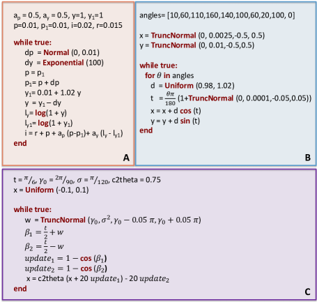
Figure 3: Probabilistic loops: (A) Taylor rule [30], (B) 2D Robotic Arm [4] (in the figure we use the inner loop as syntax sugar to keep the program compact), (C) Rimless Wheel Walker [28].

Taylor Rule Model. Central banks set monetary policy by raising or lowering their target for the federal funds rate. The Taylor rule is an equation intended to describe the interest rate decisions of central banks. The rule relates the target of the federal funds rate to the current state of the economy through the formula

$$i_{t}=r^{*}_{t}+\pi_{t}+a_{\pi}(\pi_{t}-\pi^{*}_{t})+a_{y}(y_{t}-\bar{y}_{t}),$$

where $i_{t}$ is the nominal interest rate, $r^{*}_{t}$ is the equilibrium real interest rate, $r^{*}_{t}=r$, $\pi_{t}$ is inflation rate at $t$, $\pi^{*}_{t}$ is the short-term target inflation rate at $t$, $y_{t}=\log(1+Y_{t})$, with $Y_{t}$ the real GDP, and $\bar{y}_{t}=\log(1+\bar{Y}_{t})$, with $\bar{Y}_{t}$ denoting the potential real output.

Highly-developed economies grow exponentially with a sufficiently small rate (e.g., according to the World Bank, the average growth rate of the GDP in the USA in 2001-2020 equals to 1,73%). Therefore, we set the growth rate of the potential output to 2%. Moreover, we follow [1] and model inflation as a martingale process; that is, $\mathbb{E}_{t}\left[\pi_{t+1}\right]=\pi_{t}$. The Taylor rule model is described by the program in Fig. 3, A.

Fig. 4 illustrates the performance of our approach as a function of the polynomial degree of our approximation. The approximations to the true first moment (in red) are plotted in the left panel and the relative errors for the first and second moments are in the middle and the right panels, respectively, over iteration number. The $y$-axis in both middle and right panels shows relative errors calculated as $rel.err=|est-true|/true.$ All plots show that the approximation error is low and that it deteriorates as the polynomial degree increases from 3 to 9, across iterations. The drop is sharper for the second moment.

Figure 4: The approximations and their relative errors for the Taylor rule model.

Turning Vehicle Model. The Turning vehicle model is described by the program in Fig. 1. The model was introduced in [25] and depicts the position of a vehicle, as follows. The state variables are $(x,y,v,\psi)$, where $(x,y)$ is the vehicle’s position with velocity $v$ and yaw angle $\psi$. The vehicle’s velocity is stabilized around $v_{0}=10$ m/s. The dynamics are modelled by the equations $x(t{+}1)=x(t)+\tau v\cos(\psi(t))$, $y(t{+}1)=y(t)+\tau v\sin(\psi(t))$, $v(t{+}1)=v(t)+\tau(K(v(t)-v_{0})+w_{1}(t{+}1))$, and $\psi(t{+}1)=\psi(t)+w_{2}(t{+}1)$. The disturbances $w_{1}$ and $w_{2}$ have distributions $w_{1}\sim U[-0.1,0.1]$, $w_{2}\sim N(0,0.1)$. Moreover, as in [25], we set $K=-0.5$. Initially, the state variables are distributed as: $x(0)\sim U[-0.1,0.1]$, $y(0)\sim U[-0.5,-0.3]$, $v(0)\sim U[6.5,8.0]$, $\psi(0)\sim N(0,0.01)$. We allow all normally distributed parameters take values over the entire real line, in contrast to [25] who could not accommodate distributions with infinite support and required the normal variables to take values over finite intervals.

This program requires the approximation of trigonometric functions for the computation of the location of the vehicle at time $t$. We used PCEs of degree 3, 5 and 9, built on a basic standard normal random variable, to estimate the dynamics of $x$ and $y$, the first and second coordinates of the vehicle’s location. For all three PCEs for $\sin$, the Prob-solvable loops tool estimates the first moment of $y$ to be the same, namely $-2/5$. We report the value of the first moment of $x$ in Table 1. The polynomial form of [25] can not be applied to approximate any moments of $x$ and $y$. We see that our PCE based estimate is very close to the “true” first moment of $x$, with the 9th degree PCE being the closest, as expected.

Rimless Wheel Walker. The Rimless wheel walker [25, 29] is a system that describes a human walking. The system models a rotating wheel consisting of $n_{s}$ spokes, each of length $L$, connected at a single point. The angle between consecutive spokes is $\theta=2\pi/n_{s}$. We set $L=1$ and $\theta=\pi/6.$ The Rimless wheel walker is modeled by the program in Fig. 3, C. For more details we refer to [25].

Robotic Arm Model. Proposed and studied in [4, 24, 25], this system models the position of a 2D robotic arm. The arm moves through translations and rotations. Moreover, at every step, errors in movement are modeled with probabilistic noise. The Robotic arm model is described by the program in Fig. 3, B.

Benchmark	Target	Poly form	Sim.	Deg.	Result	🕛 Runtime
Taylor rule model	$\mathbb{E}\left(i_{n}\right)$ $n{=}20$	$\times$	0.02298	$3$ $5$ $9$	$0.02278$ $0.02295$ $0.02300$	$0.4s{+}0.5s$ $0.5s{+}5.0s$ $5.9s{+}34.6s$
Turning vehicle model	$\mathbb{E}\left(x_{n}\right)$ $n{=}20$	$\times$	15.69792	$3$ $5$ $9$	$14.44342$ $15.43985$ $15.60595$	$0.6s{+}3.6s$ $1.4s{+}9.2s$ $15.6s{+}16.1s$
Turning vehicle model (trunc.)	$\mathbb{E}\left(x_{n}\right)$ $n{=}20$	for deg. 2 $\left[-3\cdot 10^{5},3\cdot 10^{5}\right]$ 1117s	15.69882	$3$ $5$ $9$	$14.44342$ $15.43985$ $15.60595$	$0.6s{+}3.6s$ $1.4s{+}9.1s$ $15.6s{+}19.0s$
Rimless wheel walker	$\mathbb{E}\left(x_{n}\right)$ $n{=}2000$	for deg. 2 $\left[1.791,1.792\right]$ 46.1s	1.79155	$1$ $2$ $3$	$1.79159$ $1.79159$ $1.79159$	$0.2s{+}0.5s$ $0.3s{+}0.5s$ $0.6s{+}0.5s$
Robotic arm model	$\mathbb{E}\left(x_{n}\right)$ $n{=}100$	for deg. 2 $\left[268.87,268.88\right]$ 35.8s	268.853	$1$ $2$ $3$	$268.85236$ $268.85227$ $268.85227$	$1.3s{+}0.3s$ $2.5s{+}0.6s$ $4.8s{+}0.7s$

Table 1: Evaluation of our approach on $4$ benchmarks. Poly form = the interval for the target as reported in [25]; Sim = target approximated through $10^{6}$ samples; Deg. = maximum degrees used for the approximation of the non-linear functions; Result = result of our method per degree; Runtime = execution time of our method in seconds (time of PCE + time of Polar).

The Rimless wheel walker and the Robotic arm model are the only two benchmarks from [25] containing non-polynomial updates. In [25], polynomial forms of degree 2 were used to compute bounding intervals for $\mathbb{E}(x_{n})$ (for fixed $n$) for the Rimless wheel walker and the Robotic arm model. Their tool does not support the approximation of logarithms (required for the Taylor rule model) and distributions with unbounded support (required for the Turning vehicle model). To facilitate comparison to polynomial forms, our set of benchmarks is augmented with a version of the Turning vehicle model using truncated normal distributions instead of normal distributions with unbounded support (Turning vehicle model (trunc.) in Table 1). We note that the technique in [25] supports more general probabilistic loops than Prob-solvable loops. However, as already mentioned in Section 2.1, we emphasize that our results in Sections 2.2-4 are not limited to Prob-solvable loops and can be applied to approximate non-linear dynamics for more general probabilistic loops.

Table 1 summarizes the evaluation of our approach on these four benchmarks and of the technique based on polynomial forms of [25] on the directly comparable Turning vehicle model (trunc.), Rimless wheel walker and the Robotic arm models. Our results illustrate that our method is able to accurately approximate general non-linear dynamics for challenging programs. Specifically, for the Rimless wheel walker model, our first moment estimate is reached upon with a first degree approximation, is close to the truth up to the fourth decimal and falls in the interval estimate of the polynomial forms technique. For the Robotic arm model, our results lie outside the interval predicted by the polynomial forms technique, yet are closer to the simulation (“truth”) calculated with $10^{6}$ samples. Moreover, our simulation agrees with the estimation provided in [25].

Our experiments also demonstrate that our method provides suitable approximations in a fraction of the time required by the technique based on polynomial forms. While polynomial forms additionally provide an error interval, they need to be computed on an iteration-by-iteration basis. In contrast, our method based on PCE and Prob-solvable loops computes an expression for the target parameterized by the loop iteration $n\in\mathbb{N}$ (cf. Fig. 1). As a result, increasing the target iteration does not increase the runtime of our approach.

Both Robotic arm and Rimless wheel walker models contain no stochastic accumulation: each basic random variable is iteration-stable and can be estimated using the scheme in Section 4.1. Therefore, for these two benchmarks, our estimation converges exponentially to the true values. On the other hand, the Taylor rule model and the Turning vehicle model contain stochasticity accumulation, which leads to the instability of the distributions of basic random variables. We apply the scheme in Section 4.2 for these two examples.

6 Conclusion

We present an approach to compute the moments of the distribution of random outputs in probabilistic loops with non-linear, non-polynomial updates. Our method is based on polynomial chaos expansion to approximate non-polynomial general functional assignments. The approximations produced by our technique have optimal exponential convergence when the parameters of the general non-polynomial functions have distributions that are stable across all iterations. We derived an upper bound on the approximation error for the case of unstable parameter distributions. Our methods can accommodate non-linear, non-polynomial updates in classes of probabilistic loops amenable to automated moment computation, such as the class of Prob-solvable loops. Moreover, our techniques can be used for moment approximation for uncertainty quantification in more general probabilistic loops. Our experiments demonstrate the ability of our methods to characterize non-polynomial behavior in stochastic models from various domains via their moments, with high accuracy and in a fraction of the time required by other state-of-the-art tools.

Appendix 0.A Proof of Theorem 4.1

Proof (Thm. 4.1)

Since $f(z)=0$ $\forall z\notin\left[a,b\right]$,

$$\left\|g(z)-\sum\limits_{i=0}^{T}c_{i}p_{i}(z)\right\|_{f}^{2}=\int\limits_{a}^{b}\left(g(z)-\sum\limits_{i=0}^{T}c_{i}p_{i}(z)\right)^{2}f(z)dz\quad$$

$$=\int\limits_{-\infty}^{\infty}\left(g(z)-\sum\limits_{i=0}^{T}c_{i}p_{i}(z)\right)^{2}f(z)dz$$

$$=\int\limits_{-\infty}^{a}\left(g(z)-\sum\limits_{i=0}^{T}c_{i}p_{i}(z)\right)^{2}f(z)dz+\int\limits_{b}^{\infty}\left(g(z)-\sum\limits_{i=0}^{T}c_{i}p_{i}(z)\right)^{2}f(z)dz$$

$$+\int\limits_{a}^{b}\left(g(z)-\sum\limits_{i=0}^{T}c_{i}p_{i}(z)\right)^{2}f(z)dz$$

$$\leq\int\limits_{-\infty}^{a}\left(g(z)-\sum\limits_{i=0}^{T}c_{i}p_{i}(z)\right)^{2}\phi(z)dz+\int\limits_{b}^{\infty}\left(g(z)-\sum\limits_{i=0}^{T}c_{i}p_{i}(z)\right)^{2}\phi(z)dz$$

$$+\int\limits_{a}^{b}\left(g(z)-\sum\limits_{i=0}^{T}c_{i}p_{i}(z)\right)^{2}\phi(z)dz+\int_{a}^{b}\left(g(z)-\sum\limits_{i=0}^{T}c_{i}p_{i}(z)\right)^{2}(f(z)-\phi(z))dz$$

$$=A+B+C+D$$ (20)

Since $f(z)-\phi(z)\leq\phi(z)+f(z)$, $D$ satisfies

$$\int\limits_{a}^{b}\left(g(z)-\sum\limits_{i=0}^{T}c_{i}p_{i}(z)\right)^{2}(f(z)-\phi(z))dz$$

$$\leq\int\limits_{a}^{b}\left(g(z)-\sum\limits_{i=0}^{T}c_{i}p_{i}(z)\right)^{2}dz\int\limits_{a}^{b}(\phi(z)+f(z))dz$$

$$=(1+\Phi(b)-\Phi(a))\times\int\limits_{a}^{b}\left(g(z)-\sum\limits_{i=0}^{T}c_{i}p_{i}(z)\right)^{2}dz,$$

with $(1+\Phi(b)-\Phi(a))<2.$ Now,

$$1\leq\frac{\phi(z)}{\min{(\phi(a),\phi(b))}}\quad\forall z\in\left[a,b\right],$$

and hence

$$\int\limits_{a}^{b}\left(g(z)-\sum\limits_{i=0}^{T}c_{i}p_{i}(z)\right)^{2}dz$$

$$\leq\min{(\phi(a),\phi(b))}^{-1}\int\limits_{a}^{b}\left(g(z)-\sum\limits_{i=0}^{T}c_{i}p_{i}(z)\right)^{2}\phi(x)dz$$

$$\leq\min{(\phi(a),\phi(b))}^{-1}C.$$ (21)

By (21) and (15), (20) satisfies

$$A+B+C+D\leq\left(\frac{2}{\min{(\phi(a),\phi(b))}}+1\right)\Bigg{\{}\int\limits_{-\infty}^{a}\left(g(z)-\sum\limits_{i=0}^{T}c_{i}p_{i}(z)\right)^{2}\phi(z)dz$$

$$+\int\limits_{b}^{\infty}\left(g(z)-\sum\limits_{i=0}^{T}c_{i}p_{i}(z)\right)^{2}\phi(z)dz+\int\limits_{a}^{b}\left(g(z)-\sum\limits_{i=0}^{T}c_{i}p_{i}(z)\right)^{2}\phi(z)dz\Bigg{\}}$$

$$=\left(\frac{2}{\min{(\phi(a),\phi(b))}}+1\right)\int\limits_{-\infty}^{\infty}\left(g(z)-\sum\limits_{i=0}^{T}c_{i}p_{i}(z)\right)^{2}\phi(z)dz$$

$$=\left(\frac{2}{\min{(\phi(a),\phi(b))}}+1\right)\sum\limits_{i=T+1}^{\infty}c_{i}^{2}\leq\left(\frac{2}{\min{(\phi(a),\phi(b))}}+1\right)\mathbb{V}\mathrm{ar}_{\phi}\left[g(Z)\right]$$

since $\mathbb{V}\mathrm{ar}_{\phi}(g(Z))=\sum_{i=1}^{\infty}c_{i}^{2}$. In consequence, the error (16) can be upper bounded by (18).

Appendix 0.B Computation Algorithm in Detail

We let ${\mathbf{D}}\in\mathbb{Z}^{L\times k}$ be the matrix with each row $j=1,\ldots,L$ containing the degrees of $Z_{i}$ (in column $i$) in the corresponding polynomial in (9). The first row corresponds to the constant polynomial (1), and the last row to $\bar{p}_{1}^{\bar{d}_{1}}(z_{1})\ldots\bar{p}_{k}^{\bar{d}_{k}}(z_{k})$. That is,

$${\mathbf{D}}=(d_{ji})_{j=1,\ldots,L,\;i=1,\ldots,k}=\blockarray{ccccc}Z_{1}&Z_{2}Z_{3}...Z_{k}\\ \block{(ccccc)}00000\\ 00001\\ \vdots\vdots\vdots\ddots\vdots\\ \bar{d}_{1}\bar{d}_{2}\bar{d}_{3}\cdots\bar{d}_{k}\\$$

The computer implementation of the algorithm computes $c_{j}$ in (10) for each $j$ combination (row) of degrees for the corresponding polynomials.

We apply the above computation to the following example. Suppose that $X$ has a truncated normal distribution with parameters $\mu=2$, $\sigma=0.1$, and is supported over $\left[1,3\right]$, and that $Y$ is uniformly distributed over $\left[1,2\right]$. We expand $g(x,y)=\log(x+y)$ along $X$ and $Y$, as follows. We choose the relevant highest degrees of expansion to be $\bar{d}_{X}=2$ and $\bar{d}_{Y}=2$. The pdf of $Y$ is $f_{Y}(y)\equiv 1$, and of $X$ is $f_{X}(x)=e^{-\frac{(x-2)^{2}}{0.02}}/0.1TrMul\sqrt{2\pi}$, where the truncation multiplier, $TrMul$, equals $\int\limits_{1}^{3}e^{-\frac{(x-2)^{2}}{0.02}}dx/0.1\sqrt{2\pi}$.

The two sets of polynomials, $\{p_{i}\}=\{1,x,x^{2}\}$ and $\{q_{i}\}=\{1,y,y^{2}\}$, are linearly independent. Applying the Gram-Schmidt procedure to orthogonalize and normalize them, we obtain $\bar{p}_{0}(x)=1$, $\bar{p}_{1}(x)=10x-20$, $\bar{p}_{2}(x)=70.71067x^{2}-282.84271x+282.13561$, and $\bar{q}_{0}(y)=1$, $\bar{q}_{1}(y)=3.4641y-5.19615$, $\bar{q}_{2}(y)=13.41641y^{2}-40.24922y+29.06888$.

In this case, $L=(1+\bar{d}_{X})*(1+\bar{d}_{Y})=9$, and ${\mathbf{D}}$ has 9 rows and 2 columns,

$${\mathbf{D}}=(d_{ji})=\blockarray{ccc}X&Y\\ \block{(cc)c}00{}\leftarrow c_{1}=\hskip 7.0pt1.2489233\\ 01{}\leftarrow c_{2}=\hskip 7.0pt0.0828874\\ 02{}\leftarrow c_{3}=-0.0030768\\ 10{}\leftarrow c_{4}=\hskip 7.0pt0.0287925\\ 11{}\leftarrow c_{5}=-0.0023918\\ 12{}\leftarrow c_{6}=\hskip 7.0pt0.0001778\\ 20{}\leftarrow c_{7}=-0.0005907\\ 21{}\leftarrow c_{8}=\hskip 7.0pt0.0000981\\ 22{}\leftarrow c_{9}=-0.0000109\\$$

Iterating through the rows of matrix ${\mathbf{D}}$ and choosing the relevant combination of degrees of polynomials for each variable, we calculate the Fourier coefficients,

$$c_{j}=\int_{1}^{3}\int_{1}^{2}log(x+y)\bar{p}_{d_{j1}}(x)\bar{q}_{d_{j2}}(y)f_{X}(x)f_{Y}(y)dydx.$$

The final estimator can be derived by summing up the products of each coefficient and the relevant combination of polynomials:

$$\log(x+y)\approx\hat{g}(x,y)=\sum_{j=1}^{9}c_{j}\bar{p}_{d_{j1}}(x)\bar{q}_{d_{j2}}(y)\approx$$

$$-0.01038x^{2}y^{2}+0.05517x^{2}y-0.10031x^{2}+$$

$$+0.06538xy^{2}-0.37513xy+0.86515x-$$

$$-0.13042y^{2}+0.93998y-0.59927.$$

The estimation error is

$$se(\hat{g})=\sqrt{\int\limits_{1}^{3}\int\limits_{1}^{2}\left(\log(x+y))-\hat{g}(x,y)\right)^{2}f_{X}(x)f_{Y}(y)dydx}\approx 0.000151895$$

Appendix 0.C PCEs of exponential and trigonometric functions

Table 2 lists examples of functions of one up to three random arguments approximated by PCE’s of different degrees and, correspondingly, number of coefficients. We use $TruncNormal(\mu,\sigma^{2},\left[a,b\right])$ to denote the truncated normal distribution with expectation $\mu$ and standard deviation $\sigma$ on the (finite or infinite) interval $\left[a,b\right]$, and $TruncGamma(\theta,k,\left[a,b\right])$ for the truncated gamma distribution on the (finite or infinite) interval $\left[a,b\right]$, $a,b>0$, with shape parameter $k$ and scale parameter $\theta$. The approximation error in (13) is reported in the last column. The results confirm (8) in practice: the error decreases as the degree or, equivalently, the number of components in the approximation of the polynomial increases.

Function	Random Variables	Degree / #coefficients	Error
$f(x_{1},x_{2})=\xi e^{-x_{1}}+(\xi-\frac{\xi^{2}}{2})e^{x_{2}-x_{1}}$ $\xi=0.3$	$x_{1}\sim Normal(0,1),$ $x_{2}\sim Normal(2,0.01)$	1 / 4 2 / 9 3 / 16 4 / 25 5 / 36	3.076846 1.696078 0.825399 0.363869 0.270419
$f(x_{1},x_{2})=0.3e^{x_{1}-x_{2}}+0.6e^{-x_{2}}$	$x_{1}\sim TruncNormal(4,1,\left[3,5\right]),$ $x_{2}\sim TruncNormal(2,0.01,\left[0,4\right])$	1 / 4 2 / 9 3 / 16 4 / 25 5 / 36	0.343870 0.057076 0.007112 0.000709 0.000059
$f(x_{1},x_{2})=e^{x_{1}x_{2}}$	$x_{1}\sim TruncNormal(4,1,\left[3,5\right])$ $x_{2}\sim TruncGamma(3,1,\left[0.5,1\right])$	1 / 4 2 / 9 3 / 16 4 / 25 5 / 36	5.745048 1.035060 0.142816 0.016118 0.001543
$f(x_{1},x_{2},x_{3})=0.3e^{x_{1}-x_{2}}+$                        $0.6e^{x_{2}-x_{3}}+0.1e^{x_{3}-x_{1}}$	$x_{1}\sim TruncNormal(4,1,\left[3,5\right])$ $x_{2}\sim TruncGamma(3,1,\left[0.5,1\right])$ $x_{3}\sim U\left[4,8\right]$	1 / 8 2 / 27 3 / 64	1.637981 0.303096 0.066869
$f(x_{1})=\psi cos(x_{1})+(1-\psi)sin(x_{1})$ $\psi=0.3$	$x_{1}\sim Normal(0,1)$	1 / 2 2 / 3 3 / 4 4 / 5 5 / 6	0.222627 0.181681 0.054450 0.039815 0.009115

Table 2: Approximations of $5$ non-linear functions using PCE.

References

- [1] Atkeson, A., Ohanian, L.E.: Are Phillips curves useful for forecasting inflation? Quarterly Review 25(Win), 2–11 (2001), https://ideas.repec.org/a/fip/fedmqr/y2001iwinp2-11nv.25no.1.html
- [2] Bartocci, E., Kovács, L., Stankovic, M.: Automatic generation of moment-based invariants for prob-solvable loops. CoRR abs/1905.02835 (2019), http://arxiv.org/abs/1905.02835
- [3] Bartocci, E., Kovacs, L., Stankovic, M.: Mora – automatic generation of moment-based invariants (2021)
- [4] Bouissou, O., Goubault, E., Putot, S., Chakarov, A., Sankaranarayanan, S.: Uncertainty propagation using probabilistic affine forms and concentration of measure inequalities. In: International Conference on Tools and Algorithms for the Construction and Analysis of Systems. pp. 225–243. Springer (2016)
- [5] Chen, X., Ábrahám, E., Sankaranarayanan, S.: Taylor model flowpipe construction for non-linear hybrid systems. In: Proc. of IEEE RTSS (2012). https://doi.org/10.1109/RTSS.2012.70
- [6] Chorin, A.J.: Gaussian fields and random flow. Journal of Fluid Mechanics 63(1), 21–32 (1974). https://doi.org/10.1017/S0022112074000991
- [7] Denamiel, C., Huan, X., Šepić, J., Vilibić, I.: Uncertainty propagation using polynomial chaos expansions for extreme sea level hazard assessment: The case of the eastern adriatic meteotsunamis. Journal of Physical Oceanography 50(4), 1005 – 1021 (2020). https://doi.org/10.1175/JPO-D-19-0147.1, https://journals.ametsoc.org/view/journals/phoc/50/4/jpo-d-19-0147.1.xml
- [8] Ernst, Oliver G., Mugler, Antje, Starkloff, Hans-Jörg, Ullmann, Elisabeth: On the convergence of generalized polynomial chaos expansions. ESAIM: M2AN 46(2), 317–339 (2012). https://doi.org/10.1051/m2an/2011045, https://doi.org/10.1051/m2an/2011045
- [9] Foo, J., Yosibash, Z., Karniadakis, G.E.: Stochastic simulation of riser-sections with uncertain measured pressure loads and/or uncertain material properties. Comput. Methods Appl. Mech. Eng. 196, 4250–4271 (2007)
- [10] Formaggia, L., Guadagnini, A., Imperiali, I., Lever, V., Porta, G., Riva, M., Scotti, A., Tamellini, L.: Global sensitivity analysis through polynomial chaos expansion of a basin-scale geochemical compaction model. Comput. Geosci. 17, 25–42 (2013)
- [11] Ghanem, R., Dham, S.: Stochastic finite element analysis for multiphase flow in heterogeneous porous media. Transport in Porous Medias 32, 239–262 (1998), https://doi.org/10.1023/A:1006514109327
- [12] Ghanem, R.: Probabilistic characterization of transport in heterogeneous media. Computer Methods in Applied Mechanics and Engineering 158, 199–220 (1998), doi:10.1016/s0045-7825(97)00250-8
- [13] Ghanem, R.G., Spanos, P.D.: Stochastic Finite Elements: A Spectral Approach. Springer, New York, NY (1991)
- [14] Giraldi, L., Maître, O.P.L., Mandli, K.T., Dawson, C.N., Hoteit, I., Knio, O.M.: Bayesian inference of earthquake parameters from buoy data using a polynomial chaos-based surrogate. Comput. Geosci. 21, 683–699 (2017)
- [15] Hien, T.D., Kleiber, M.: Stochastic finite element modelling in linear transient heat transfer. Computer Methods in Applied Mechanics and Engineering 144(1), 111–124 (1997). https://doi.org/https://doi.org/10.1016/S0045-7825(96)01168-1, https://www.sciencedirect.com/science/article/pii/S0045782596011681
- [16] Hou, T.Y., Luo, W., Rozovskii, B., Zhou, H.M.: Wiener chaos expansions and numerical solutions of randomly forced equations of fluid mechanics. J. Comput. Phys. 216, 687–706 (2006)
- [17] Jasour, A., Wang, A., Williams, B.C.: Moment-based exact uncertainty propagation through nonlinear stochastic autonomous systems. CoRR abs/2101.12490 (2021), https://arxiv.org/abs/2101.12490
- [18] Knio, O.M., Maître, O.P.L.: Uncertainty propagation in CFD using polynomial chaos decomposition. Fluid Dynamics Research 38(9), 616–640 (sep 2006). https://doi.org/10.1016/j.fluiddyn.2005.12.003, https://doi.org/10.1016/j.fluiddyn.2005.12.003
- [19] Makino, K., Berz, M.: Taylor models and other validated functional inclusion methods. Int. J. Pure Appl. Math (2003)
- [20] Meecham, W.C., Jeng, D.T.: Use of the Wiener—Hermite expansion for nearly normal turbulence. Journal of Fluid Mechanics 32(2), 225–249 (1968). https://doi.org/10.1017/S0022112068000698
- [21] Moosbrugger, M., Stankovič, M., Bartocci, E., Kovács, L.: This is the Moment for Probabilistic Loops. arXiv (2022)
- [22] Mühlpfordt, T., Findeisen, R., Hagenmeyer, V., Faulwasser, T.: Comments on truncation errors for polynomial chaos expansions. IEEE Control Systems Letters 2(1), 169–174 (2018). https://doi.org/10.1109/LCSYS.2017.2778138
- [23] Neher, M., Jackson, K.R., Nedialkov, N.S.: On taylor model based integration of odes. SIAM Journal on Numerical Analysis pp. 236–262 (2007). https://doi.org/10.1137/050638448
- [24] Sankaranarayanan, S.: Quantitative analysis of programs with probabilities and concentration of measure inequalities. Foundations of Probabilistic Programming p. 259 (2020)
- [25] Sankaranarayanan, S., Chou, Y., Goubault, E., Putot, S.: Reasoning about uncertainties in discrete-time dynamical systems using polynomial forms. In: Larochelle, H., Ranzato, M., Hadsell, R., Balcan, M.F., Lin, H. (eds.) Advances in Neural Information Processing Systems. vol. 33, pp. 17502–17513. Curran Associates, Inc. (2020), https://proceedings.neurips.cc/paper/2020/file/ca886eb9edb61a42256192745c72cd79-Paper.pdf
- [26] Son, J., Du, Y.: Probabilistic surrogate models for uncertainty analysis: Dimension reduction-based polynomial chaos expansion. International Journal for Numerical Methods in Engineering 121(6), 1198–1217 (2020). https://doi.org/https://doi.org/10.1002/nme.6262, https://onlinelibrary.wiley.com/doi/abs/10.1002/nme.6262
- [27] Stanković, B.: Taylor expansion for generalized functions. Journal of Mathematical Analysis and Application 203, 31-37 (1996)
- [28] Steinhardt, J., Tedrake, R.: Finite-time regional verification of stochastic non-linear systems. Int. J. Robotics Res. 31(7), 901–923 (2012). https://doi.org/10.1177/0278364912444146
- [29] Steinhardt, J., Tedrake, R.: Finite-time regional verification of stochastic non-linear systems. The International Journal of Robotics Research 31(7), 901–923 (2012)
- [30] Taylor, J.B.: Discretion versus policy rules in practice. Carnegie-Rochester Conference Series on Public Policy 39(1), 195–214 (December 1993), https://ideas.repec.org/a/eee/crcspp/v39y1993ip195-214.html
- [31] Triebel, H.: Taylor expansions of distributions. In: The Structure of Functions. Birkhäuser Basel (2001). https://doi.org/10.1007/978-3-0348-8257-6_8
- [32] Wan, X., Karniadakis, G.E.: An adaptive multi-element generalized polynomial chaos method for stochastic differential equations. J. Comput. Phys. 209, 617–642 (2005)
- [33] Xiu, D.: Numerical Methods for Stochastic Computations: A Spectral Method Approach. Princeton University Press (2010), http://www.jstor.org/stable/j.ctv7h0skv
- [34] Xiu, D., Karniadakis, G.E.: The Wiener-Askey polynomial chaos for stochastic differential equations. SIAM J. Sci. Comput. 24(2), 619–644 (Feb 2002). https://doi.org/10.1137/S1064827501387826