A Boosted-DCA with Power-Sum-DC Decomposition for Linearly Constrained Polynomial Program

Abstract

In this paper, we introduce a difference-of-convex (DC) decomposition for polynomials based on power-sum representation, which can be established by solving a sparse linear system. A boosted DCA with exact line search (BDCAe) is proposed to solve the DC formulation of the linearly constrained polynomial program. We show that the exact line search is equivalent to finding roots of a unary polynomial in an interval, which has a closed-form solution in many applications. The subsequential convergence of BDCAe to a critical point is proved, and the convergence rate under Kurdyka-Łojasiewicz property is established. Moreover, a fast dual proximal gradient (FDPG) method is applied to efficiently solve the resulting convex subproblems. Numerical experiments on the Mean-Variance-Skewness-Kurtosis (MVSK) portfolio optimization model via BDCAe, DCA, BDCA with Armijo line search, as well as FMINCON and FILTERSD solvers are reported, which demonstrates good performance of BDCAe.

1 Introduction

We are interested in solving the polynomial optimization problem with linear constraints:

$$\min_{\mathbf{x}\in\mathcal{\mathcal{P}}}f(\mathbf{x}),$$ (POPL)

where $f$ is a multivariate polynomial and $\mathcal{P}$ is a nonempty convex polyhedral set (not necessarily bounded), defined by

$$\mathcal{P}:=\{\mathbf{x}\in\mathbb{R}^{n}:\langle\boldsymbol{a}_{i},\mathbf{x}\rangle\leq b_{i},\langle\boldsymbol{p}_{j},\mathbf{x}\rangle=q_{j},i=1,\cdots,m,j=1,\cdots,r\}$$

where $\mathbf{a}_{i},\mathbf{p}_{j}\in\mathbb{R}^{n}$ and $b_{i},q_{j}\in\mathbb{R}$. Throughout the paper, we use a bold face letter as $\mathbf{x}$ for a vector and $\mathbf{x}_{i}$ for the i-th coordinate of the vector $\mathbf{x}$. The polynomial function $f$ is assumed to be bounded from below over $\mathcal{P}$, i.e.,

$$\inf_{\mathbf{x}\in\mathcal{P}}f(\mathbf{x})>-\infty.$$

This problem arises in many applications such as the higher-order moment portfolio selection dinh2016dc ; Niu2011 ; niu2019higher , the eigenvalue complementarity problem le2012dc ; niu2013efficient ; niu2015solving ; niu2019improved , the tensor complementarity problem song2016properties , the Euclidean distance matrix completion problem bakonyi1995euclidian , the copositivity of matrix bras2016copositivity ; burer2009copositive ; dur2013testing ; you2022refined , the Boolean polynomial program niu2019discrete , the linear and bilinear matrix inequalities boyd1994linear ; niu2014dc , and so on.

The (POPL) is indeed a special class of the difference-of-convex (DC) program hartman1959functions ; hiriart1985generalized ; le2018dc , defined as below:

$$\min_{\mathbf{x}\in\mathcal{\mathcal{P}}}\{f(\mathbf{x}):=g(\mathbf{x})-h(\mathbf{x})\}, {}_{\text{dc}}$$ (P)

where $g$ and $h$ are convex polynomials. There are some related works on DC decompositions for polynomials. The DC decomposition for quadratic functions has been studied in hoai2000efficient ; bomze2004undominated ; le1997solving based on the eigenvalue decomposition of real symmetric matrices. However, in the case of general multivariate polynomials, this technique is no longer available and the DC decomposition is more difficult to obtain (especially in dense polynomials). Niu et al. Niu2011 proposed a DC decomposition for general polynomials in the form of $\frac{\sigma}{2}\|\mathbf{x}\|^{2}-(\frac{\sigma}{2}\|\mathbf{x}\|^{2}-f)$ where $\sigma>0$ is obtained by estimating an upper bound of the spectral radius of the Hessian matrix of $f$ over a compact convex set. This technique has been successfully applied to several real-world applications such as the higher-order moment portfolio optimization Niu2011 and the eigenvalue complementarity problems niu2013efficient ; niu2015solving ; niu2019improved . Ahmadi et al. ahmadi2018dc explored DC decompositions for polynomials via algebraic relaxation techniques. They showed in ahmadi2012convex that convexity is different from sos-convexity, and characterized the discrepancy between convexity and sos-convexity in ahmadi2013complete for polynomials. Several DC decompositions are proposed in ahmadi2018dc by solving linear, second-order cone, or semidefinite programs. Meanwhile, Niu defined in niu2018difference the so-called Difference-of-Convex-Sums-of-Squares (DC-SOS) decomposition for general polynomials and developed several practical DC-SOS decomposition techniques. Some of these decomposition techniques can be also parallelized. The DC decomposition technique proposed in this paper is indeed a special DC-SOS decomposition in form of power-sums of linear forms, namely the power-sum DC (PSDC) decomposition. We will show that this decomposition can be established by solving a sparse linear system, which is discussed in Section 3.

Concerning the solution method for DC programming formulation (P${}_{\text{dc}}$), the most popular method is DCA, introduced by Pham 1988Duality in 1985 as an extension of the subgradient method, and extensively developed by Le Thi and Pham since 1994 (see, e.g., le1997solving ; tao2005dc ; le2018dc ; 1997Convex ; tao1998dc and the references therein). The main idea of DCA is to minimize a sequence of convex majorizations of the DC objective function $f$ by linearizing the second DC component $h$ at the current iterate. The general convergence theorem of DCA ensures that every limit point of the generated sequence $\{\mathbf{x}^{k}\}$ by DCA is a critical point of (P${}_{\text{dc}}$) (see, e.g., 1997Convex ; tao2005dc ). Recent years, some accelerated DCAs are established. Artacho et al. artacho2018accelerating proposed a boosted DCA (BDCA) by incorporating DCA with an Armijo-type line search to potentially accelerate DCA under the smoothness assumption of both $g$ and $h$. This method is extended to the non-smooth case of $h$ component in aragon2018boosted . Meanwhile, Niu et al. niu2019higher further extended BDCA to the convex constrained DC program for both smooth and nonsmooth cases. The global convergence theorem is established under the Łojasiewicz subgradient inequality. Besides, some other accelerations based on the heavy-ball method polyak1964some and Nesterov’s extrapolation nesterov1983method are also proposed. The inertial DCA (InDCA) de2019inertial is established by de Oliveira as a heavy-ball type polyak1964some accelerated DCA. Le Thi et al. proposed in nhat2018accelerated a Nesterov-type accelerated DCA (ADCA). Wen et al. wen2018proximal proposed a proximal DCA algorithm with Nesterov-type extrapolation gotoh2018dc . In this paper, based on BDCA for convex constrained DC program established in niu2019higher , we introduce an exact line search to accelerate DCA for solving (POPL), namely BDCA${}_{\text{e}}$. The exact line search is equivalent to searching roots of a unary polynomial in an interval, which has a closed-form solution in many applications. We provide a verifiable necessary and sufficient condition for checking the feasibility of the line search direction (namely, the DC descent direction, generated by two consecutive iterates of DCA), and an upper bound for the initial stepsize along the DC descent direction is estimated. Moreover, a fast dual proximal gradient (FDPG) method beck2017first is proposed to effectively solve the convex subproblems in DCA and BDCA${}_{\text{e}}$ by exploiting the special structure of the power-sum DC decomposition. The convergence of BDCA${}_{\text{e}}$ is proved and its convergence rate under the Kurdyka-Łojasiewicz property is established.

The rest of this paper is organized as follows. In Section 2, we recall some notations and preliminaries required in this paper. In Section 3, we establish two power-sum DC decompositions to get two DC programming formulations of (POPL). The corresponding BDCA${}_{\text{e}}$ to the two DC formulations are proposed in Section 4. The convergence analysis and the convergence rate of BDCA${}_{\text{e}}$ are proved in Section 5. The FDPG method for solving the convex subproblem are presented in Section 6. Some numerical experiments on the Mean-Variance-Skewness-Kurtosis portfolio optimization model by comparing BDCA${}_{\text{e}}$ with the classical DCA, BDCA with the Armijo line search, as well as the solvers FILTERSD and FMINCON are reported in Section 7. Some concluding remarks and potential research topics are discussed in the final section.

2 Notations and preliminaries

The inner product of two vectors $\mathbf{x},\mathbf{y}\in\mathbb{R}^{n}$ is denoted by $\langle\mathbf{x},\mathbf{y}\rangle$, while $\|\cdot\|$ denotes the induced norm, defined by $\|\mathbf{x}\|=\sqrt{\langle\mathbf{x},\mathbf{x}\rangle}.$ The gradient of a differentiable function $f:\mathbb{R}^{n}\rightarrow\mathbb{R}$ at $\mathbf{x}^{0}\in\mathbb{R}^{n}$ is denoted by $\nabla f(\mathbf{x}^{0})\in\mathbb{R}^{n}$.

A function $f:\mathbb{R}^{n}\rightarrow\mathbb{R}$ is said to be $\rho$-strongly convex ($\rho>0$) if

$$f(\lambda\mathbf{x}+(1-\lambda)\mathbf{y})\leq\lambda f(\mathbf{x})+(1-\lambda)f(\mathbf{y})-\frac{\rho}{2}\lambda(1-\lambda)\|\mathbf{x}-\mathbf{y}\|^{2}$$

for all $\mathbf{x},\mathbf{y}\in\mathbb{R}^{n}$ and $\lambda\in]0,1[,$ which is equivalent to that $f-\frac{\rho}{2}\|\cdot\|^{2}$ is convex. A function $\psi:\mathbb{R}^{n}\rightarrow\mathbb{R}^{n}$ is called Lipschitz continuous, if there is some constant $L>0$ such that

$$\|\psi(\mathbf{x})-\psi(\mathbf{y})\|\leq L\|\mathbf{x}-\mathbf{y}\|\text{ for all }\mathbf{x},\mathbf{y}\in\mathbb{R}^{n}$$

and $\psi$ is said to be locally Lipschitz continuous if, for each $\mathbf{x}\in\mathbb{R}^{n}$, there exists a neighborhood $\mathcal{U}$ of $\mathbf{x}$ such that $\psi$ restricted to $\mathcal{U}$ is Lipschitz continuous.

The definition of the cone of feasible directions at $\bar{\mathbf{y}}\in\mathcal{P}$ is defined as

$$\mathcal{D}(\bar{\mathbf{y}}):=\{\mathbf{d}\in\mathbb{R}^{n}:\text{ there exists }\delta>0\text{ such that }\bar{\mathbf{y}}+t\mathbf{d}\in\mathcal{P},\forall t\in[0,\delta]\}$$

and the set of active constraints at $\bar{\mathbf{y}}$ is denoted by

$$\mathcal{A}(\bar{\mathbf{y}})=\{i\in\{1,\cdots,m\}:\langle\mathbf{a}_{i},\bar{\mathbf{y}}\rangle=b_{i}\}.$$

Then, it is classical (see, e.g., (aragon2019nonlinear, , Proposition 4.14)) to get the next equality

$$\mathcal{D}(\bar{\mathbf{y}})=\{\mathbf{d}\in\mathbb{R}^{n}:\langle\mathbf{a}_{i},\mathbf{d}\rangle\leq 0,\langle\mathbf{p}_{j},\mathbf{d}\rangle=0,i\in\mathcal{A}(\bar{\mathbf{y}}),j=1,\cdots,r\}.$$

Let $\Gamma_{0}(\mathbb{R}^{n})$ be the set of all extended real-valued proper closed convex functions from $\mathbb{R}^{n}$ to $(-\infty,+\infty]$. A function $f:\mathbb{R}^{n}\rightarrow(-\infty,+\infty]$ is said to be difference-of-convex (DC) if $f=g-h$ with $g,h\in\Gamma_{0}(\mathbb{R}^{n})$. We call that $g$ and $h$ are DC components of $f$ and $g-h$ is a DC decomposition of $f$.

For a proper and closed (or lower semicontinuous) function $f:\mathbb{R}^{n}\rightarrow(-\infty,+\infty]$, the Fréchet subdifferential of $f$ at $\mathbf{x}_{0}\in\text{dom}f:=\{\mathbf{x}\in\mathbb{R}^{n}:f(\mathbf{x})<+\infty\}$ is defined by

$$\partial^{F}f(\mathbf{x}_{0})=\{\mathbf{u}\in\mathbb{R}^{n}:\liminf_{\mathbf{h}\rightarrow\mathbf{0}}\dfrac{f(\mathbf{x}_{0}+\mathbf{h})-f(\mathbf{x}_{0})-\langle\mathbf{u},\mathbf{h}\rangle}{\|\mathbf{h}\|}\geq 0\},$$

and if $\mathbf{x}_{0}\notin\text{dom}f$, then we take $\partial^{F}f(\mathbf{x}_{0})=\emptyset.$ A point $\mathbf{x}_{0}\in\mathbb{R}^{n}$ is called a (Fréchet) critical point for $f$, if $0\in\partial^{F}f(\mathbf{x}_{0}).$ The effective domain of $\partial^{F}f$ is defined by

$$\text{dom}(\partial^{F}f):=\{\mathbf{x}\in\text{dom}f:\partial^{F}f(\mathbf{x})\neq\emptyset\}.$$

Particularly, when $f$ is convex, then $\partial^{F}f$ coincides with the classical subdifferential in convex analysis, defined by

$$\partial f(\mathbf{x}_{0})=\{\mathbf{u}\in\mathbb{R}^{n}:f(\mathbf{x})-f(\mathbf{x}_{0})\geq\langle\mathbf{u},\mathbf{x}-\mathbf{x}_{0}\rangle,\forall\mathbf{x}\in\mathbb{R}^{n}\}.$$

Moreover, if $f$ is a DC function with $f=g-h$, and $h$ is differentiable at $\mathbf{x}$, then one has the following equality:

$$\partial^{F}f(\mathbf{x})=\partial g(\mathbf{x})-\nabla h(\mathbf{x}).$$

Let $\chi_{\mathcal{P}}:\mathbb{R}^{n}\to(-\infty,+\infty]$ be the indicator function of the polyhedral convex set $\mathcal{P}$ defined by $\chi_{\mathcal{P}}(\mathbf{x})=0$ if $\mathbf{x}\in\mathcal{P}$ and $\chi_{\mathcal{P}}(\mathbf{x})=+\infty$ if $\mathbf{x}\notin\mathcal{P}$. Then $\chi_{\mathcal{P}}$ belongs to $\Gamma_{0}(\mathbb{R}^{n})$ and $\partial\chi_{\mathcal{P}}(\mathbf{x})=\mathcal{N}_{\mathcal{P}}(\mathbf{x})$ where $\mathcal{N}_{\mathcal{P}}(\mathbf{x})$ is the normal cone to $\mathcal{P}$ at $\mathbf{x}$ defined by

$$\mathcal{N}_{\mathcal{P}}(\mathbf{x}):=\{\mathbf{v}\in\mathbb{R}^{n}:\langle\mathbf{v},\mathbf{y}-\mathbf{x}\rangle,\forall\mathbf{y}\in\mathcal{P}\}.$$

A point $\mathbf{x}_{0}$ is a (Fréchet) critical point of (P${}_{\text{dc}}$) with differentiable $h$ at $\mathbf{x}_{0}$ iff

$$\nabla h(x_{0})\in\nabla g(\mathbf{x}_{0})+\mathcal{N}_{\mathcal{P}}(\mathbf{x}_{0}).$$

The set of real polynomials with degree up to $d$ in $n$ variables $\mathbf{x}\in\mathbb{R}^{n}$ is denoted by $\mathbb{R}_{d}[\mathbf{x}]$. The set of all $n$-variate and $d$-degree homogeneous polynomials (forms) is defined by $\mathbb{H}_{d}[\mathbf{x}]$, i.e.,

$$\mathbb{H}_{d}[\mathbf{x}]:=\{f(\mathbf{x})\in\mathbb{R}_{d}[\mathbf{x}]:f(\mathbf{x})=\sum_{\boldsymbol{\alpha}\in\mathcal{I}_{n,d}}c_{\boldsymbol{\alpha}}{\mathbf{x}}^{\boldsymbol{\alpha}}\},$$

where $\mathcal{I}_{n,d}=\{\boldsymbol{\alpha}=(\alpha_{1},\cdots,\alpha_{n})^{\top}\in\mathbb{N}^{n}:\sum_{i=1}^{n}\alpha_{i}=d\}$ and $c_{\boldsymbol{\alpha}}\in\mathbb{R}$. Let us denote by $s_{n,d}=\tbinom{n+d-1}{d}$ the cardinality of $\mathcal{I}_{n,d}$ and rewrite $\mathcal{I}_{n,d}$ as $\mathcal{I}_{n,d}=\{\boldsymbol{\alpha}_{1},\boldsymbol{\alpha}_{2},\cdots,\boldsymbol{\alpha}_{s_{n,d}}\}$.

A form $f(\mathbf{x})\in\mathbb{H}_{d}[\mathbf{x}]$ is said to have a power-sum representation, if there exist linear forms $L_{i}(\mathbf{x})\in\mathbb{H}_{1}[\mathbf{x}]$ and scalars $\lambda_{i}\in\mathbb{R}$ ($i=1,\cdots,r$) such that

$$f(\mathbf{x})=\sum_{i=1}^{r}\lambda_{i}L_{i}^{d}(\mathbf{x}),\forall\mathbf{x}\in\mathbb{R}^{n}.$$

A proper and closed function $f:\mathbb{R}^{n}\to(-\infty,+\infty]$ is said to have the Kurdyka–Łojasiewicz property at $\mathbf{x}^{*}\in\text{dom}(\partial^{F}f)$ if there exist $\eta\in(0,+\infty)$, a concave function $\varphi:[0,\eta]\rightarrow[0,+\infty)$ and a neighborhood $\mathcal{U}$ of $\mathbf{x}^{*}$, such that

1. $\varphi(0)=0;$

2. $\varphi$ belongs to the class $\mathscr{C}^{1}$ on $(0,\eta);$

3. $\varphi^{\prime}>0$ on $(0,\eta);$

4. $\forall\mathbf{x}\in\mathcal{U}$ with $f(\mathbf{x}^{*})<f(\mathbf{x})<f(\mathbf{x}^{*})+\eta$, we have the KL inequality

   $$\varphi^{\prime}(f(\mathbf{x})-f(\mathbf{x}^{*}))\text{dist}(0,\partial^{F}f(\mathbf{x}))\geq 1.$$

The class of functions having the KL property is very ample. For example, all semialgebraic and subanalytic functions satisfy the KL inequality bolte2007lojasiewicz ; kurdyka1994wf ; lojasiewicz1993geometrie , so as to polynomial functions and indicator functions of polyhedral sets.

3 Power-Sum-DC decompositions of polynomials

3.1 Power-sum representation

It is known (see, e.g., trove ) that any form can be represented as weighted power-sum of linear forms (cf. the power-sum representation). For a given form, its power-sum representation (if exists) is not unique in general and nontrivial to be constructed. This kind of representations dates back to the Waring decomposition of homogeneous polynomials in complex space, defined as finding the smallest positive integer $r$ for a power-sum representation of a polynomial, which is notoriously difficult to determine in general. To date, only a few particular families are known (see, e.g., buczynska2013waring ; carlini2012solution ; mella2009base ). The situation in the real case is more complicated blekherman2015typical , and little is known. In the next lemma, we have a power-sum representation of a form by solving a linear system.

Lemma 1

For any form $f(\mathbf{x})\in\mathbb{H}_{d}[\mathbf{x}]$, i.e., $f(\mathbf{x})=\sum_{\boldsymbol{\alpha}\in\mathcal{I}_{n,d}}c_{\boldsymbol{\alpha}}{\mathbf{x}}^{\boldsymbol{\alpha}},$ one has the following power-sum representation for some $\lambda_{\boldsymbol{\alpha}}\in\mathbb{R}$:

$$f(\mathbf{x})=\sum_{\boldsymbol{\alpha}\in\mathcal{I}_{n,d}}\lambda_{\boldsymbol{\alpha}}\langle\boldsymbol{\alpha},\mathbf{x}\rangle^{d}.$$ (1)

Proof

Let $\mathbf{x}\in\mathbb{R}^{n}$, the multinomial equation reads as

$$\bigg{(}\sum_{i=1}^{n}x_{i}\bigg{)}^{d}=\sum_{\boldsymbol{\alpha}\in\mathcal{I}_{n,d}}{d\choose\boldsymbol{\alpha}}\mathbf{x}^{\boldsymbol{\alpha}},$$ (2)

where ${d\choose\boldsymbol{\alpha}}=\frac{d!}{\alpha_{1}!\alpha_{2}!\cdots\alpha_{n}!}$. It follows from

$$\langle\boldsymbol{\alpha},\mathbf{x}\rangle^{d}=\sum_{\boldsymbol{\beta}\in\mathcal{I}_{n,d}}{d\choose\boldsymbol{\beta}}\boldsymbol{\alpha}^{\boldsymbol{\beta}}\mathbf{x}^{\boldsymbol{\beta}},\forall\boldsymbol{\alpha}\in\mathcal{I}_{n,d},$$

that

$$\begin{pmatrix}\langle\boldsymbol{\alpha}_{1},\mathbf{x}\rangle^{d}\\ \langle\boldsymbol{\alpha}_{2},\mathbf{x}\rangle^{d}\\ \vdots\\ \langle\boldsymbol{\alpha}_{s_{n,d}},\mathbf{x}\rangle^{d}\end{pmatrix}=\mathbf{D}(n,d)\begin{pmatrix}\mathbf{x}^{\boldsymbol{\alpha}_{1}}\\ \mathbf{x}^{\boldsymbol{\alpha}_{2}}\\ \vdots\\ \mathbf{x}^{\boldsymbol{\alpha}_{s_{n,d}}}\end{pmatrix},$$ (3)

where the matrix

$$\mathbf{D}(n,d)=\bigg{(}\tbinom{d}{\boldsymbol{\alpha}_{j}}(\boldsymbol{\alpha}_{i})^{\boldsymbol{\alpha}_{j}}\bigg{)}_{1\leq i,j\leq s_{n,d}}.$$

Let $\mathcal{B}=(\mathbf{x}^{\boldsymbol{\alpha}_{1}},\mathbf{x}^{\boldsymbol{\alpha}_{2}},\cdots,\mathbf{x}^{\boldsymbol{\alpha}_{s_{n,d}}})^{\top}$ and $\widetilde{\mathcal{B}}=(\langle\boldsymbol{\alpha}_{1},\mathbf{x}\rangle^{d},\langle\boldsymbol{\alpha}_{2},\mathbf{x}\rangle^{d},\cdots,\langle\boldsymbol{\alpha}_{s_{n,d}},\mathbf{x}\rangle^{d})^{\top}$. Then by the nonsingularity of $\mathbf{D}(n,d)$ niu2021power ; shelton1986multinomial , we can rewrite (3) as

$$\mathcal{B}=\mathbf{D}^{-1}(n,d)\widetilde{\mathcal{B}}.$$

Let $\mathbf{c}=(c_{\boldsymbol{\alpha}_{1}},\cdots,c_{\boldsymbol{\alpha}_{s_{n,d}}})^{\top}$. Then

$$f(\mathbf{x})=\boldsymbol{c}^{\top}\mathcal{B}=\boldsymbol{c}^{\top}\mathbf{D}^{-1}(n,d)\widetilde{\mathcal{B}}=\boldsymbol{\lambda}^{\top}\widetilde{\mathcal{B}}$$

with $\boldsymbol{\lambda}=(\mathbf{D}^{-1}(n,d))^{\top}\boldsymbol{c}$. ∎

Remark 1

Lemma 1 indicates that a power-sum representation of a form can be generated by solving the linear system:

$$\mathbf{D}(n,d)\boldsymbol{\lambda}=\boldsymbol{c}.$$ (4)

$\mathbf{D}(n,d)$ is asymmetric in general and the size of $\mathbf{D}(n,d)$ is $\tbinom{n+d-1}{d}^{2}$, which could be very large even if $n$ and $d$ are not too large. For instance, when $d=4$ and $n=100$, the size of $\mathbf{D}(n,d)$ goes up to millions. Fortunately, in many applications of polynomial optimization, the number of variables $n$ is much bigger than the degree $d$, in this case, the matrix $\mathbf{D}(n,d)$ appears to be very sparse, whose analysis is demonstrated in niu2021power . As a consequence, the density of the matrix $\mathbf{D}(n,d)$ goes to $0$ as $n\rightarrow+\infty$ for any fixed $d$. In Fig. 1, we observe that for $n>6$, the sparsity of $\mathbf{D}(n,d)$ with $d=3,4,5$ respectively is more than $90\%$. Thanks to the sparsity of the matrix $\mathbf{D}(n,d)$, the power-sum representation of a form can be generated effectively by solving the sparse linear system (4).

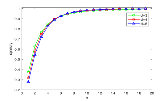
Figure 1: The sparsity of the matrix $\mathbf{D}(n,d)$ v.s. $n$ for $d=3,4,5$.

3.2 Power-sum difference-of-convex decompositions

In this section, we establish the DC decomposition for any polynomial in two ways: the termwise power-sum-DC (TPSDC) decomposition and the homogenizing-dehomogenizing power-sum-DC (HDPSDC) decomposition.

TPSDC decomposition

: Applying Lemma 1 to a form, we can establish a power-sum-DC (PSDC) decomposition of any homogeneous polynomial in two cases: odd degree forms and even degree forms.

Corollary 1

Let $f(\mathbf{x})\in\mathbb{H}_{d}[\mathbf{x}]$.

• If the degree $d$ is even, then we have a PSDC decomposition as

  $$f(\mathbf{x})=\sum_{\boldsymbol{\alpha}\in\mathcal{I}^{+}}\lambda_{\boldsymbol{\alpha}}\langle\boldsymbol{\alpha},\mathbf{x}\rangle^{d}-\sum_{\boldsymbol{\alpha}\in\mathcal{I}^{-}}(-\lambda_{\boldsymbol{\alpha}})\langle\boldsymbol{\alpha},\mathbf{x}\rangle^{d},$$ (5)

  where $\mathcal{I}^{+}=\{\boldsymbol{\alpha}\in\mathcal{I}_{n,d}:\lambda_{\boldsymbol{\alpha}}>0\}$ and $\mathcal{I}^{-}=\{\boldsymbol{\alpha}\in\mathcal{I}_{n,d}:\lambda_{\boldsymbol{\alpha}}<0\}.$

• If the degree $d$ is odd, then we have a PSDC decomposition as

  $$f(\mathbf{x})=\sum_{\boldsymbol{\alpha}\in\mathcal{I}^{+}}\lambda_{\boldsymbol{\alpha}}\langle\boldsymbol{\alpha},\hat{\mathbf{x}}\rangle^{d+1}-\sum_{\boldsymbol{\alpha}\in\mathcal{I}^{-}}(-\lambda_{\boldsymbol{\alpha}})\langle\boldsymbol{\alpha},\hat{\mathbf{x}}\rangle^{d+1},$$ (6)

  where $\mathcal{I}^{+}=\{\boldsymbol{\alpha}\in\mathcal{I}_{n+1,d+1}:\lambda_{\boldsymbol{\alpha}}>0\},\mathcal{I}^{-}=\{\boldsymbol{\alpha}\in\mathcal{I}_{n+1,d+1}:\lambda_{\boldsymbol{\alpha}}<0\}$ and $\hat{\mathbf{x}}=(\mathbf{x},1).$

Proof

The case (i) is followed by Lemma 1. To prove the case (ii), we can multiply $f(\mathbf{x})$ with an additional variable $x_{n+1}$ to get an even degree form $\tilde{f}(\tilde{\mathbf{x}})=x_{n+1}f(\mathbf{x})$. Then, by applying the case (i) to $\tilde{f}(\tilde{x})$ and setting $x_{n+1}=1$, we get immediately the case (ii). ∎

Any polynomial $f(\mathbf{x})\in\mathbb{R}_{d}[\mathbf{x}]$ can be written as a finite sum of forms $f(\mathbf{x})=\sum_{k=0}^{d}h_{k}(\mathbf{x})$ with $h_{k}(\mathbf{x})\in\mathbb{H}_{k}[\mathbf{x}](k=0,1,\cdots,d).$ Hence, applying Corollary 1 to each forms $h_{k}(\mathbf{x})(k=1,2,\cdots,d)$, we obtain a so-called termwise power-sum (TPSDC) decomposition of $f(\mathbf{x})$, which is described in Algorithm 1.

Input: $h_{1}(\mathbf{x}),\cdots,h_{d}(\mathbf{x})$;

1 $\mathcal{K_{\boldsymbol{\lambda}}}\leftarrow\emptyset,\mathcal{K_{\mathcal{I}}}\leftarrow\emptyset$;

2 for $k=1,\cdots,d$ do

3       if $k$ is odd then

4             $\hat{n}\leftarrow n+1,\hat{d}\leftarrow k+1;$

5            

6      else

7            $\hat{n}\leftarrow n,\hat{d}\leftarrow k;$

8       end if

9      $\mathcal{I}\leftarrow\mathcal{I}_{\hat{n},\hat{d}}$;

10       $\boldsymbol{c}\leftarrow$ the coefficient of $h_{k}(\mathbf{x})$ associated with canonical basis generated by set $\mathcal{I}$;

11       Compute $\boldsymbol{\lambda}$ by solving linear equations: $\mathbf{D}^{\top}(\hat{n},\hat{d})\boldsymbol{\lambda}=\boldsymbol{c}$;

12       $\mathcal{K_{\boldsymbol{\lambda}}}\leftarrow\mathcal{K_{\boldsymbol{\lambda}}}\cup\boldsymbol{\lambda},\mathcal{K_{\mathcal{I}}}\leftarrow\mathcal{K_{\mathcal{I}}}\cup\mathcal{I};$

13      

14 end for

15return $\mathcal{K_{\boldsymbol{\lambda}}}$ and $\mathcal{K_{\mathcal{I}}}$;

Algorithm 1 TPSDC Decomposition

HDPSDC decomposition

: It is well-known that: an $n$-variate $d$-degree form can be dehomogenized to a polynomial in $n-1$ variable of degree not more than $d$ by fixing a variable to 1 (cf. dehomogenization); conversely, a polynomial can be converted into a form by multiplying some powers of a new variable $x_{n+1}$ to each monomial as $f_{H}(\tilde{\mathbf{x}})=x_{n+1}^{d}\ f(x_{1}/x_{n+1},\cdots,x_{n}/x_{n+1})$ (cf. homogenization). Based on this fact, we propose a PSDC representation for any polynomial as follows:

Proposition 1

For any polynomial $f(\mathbf{x})\in\mathbb{R}_{d}[\mathbf{x}]$, one has the following PSDC decomposition:

$$f(\mathbf{x})=\sum_{\boldsymbol{\alpha}\in\mathcal{I}^{+}}\lambda_{\boldsymbol{\alpha}}\langle\boldsymbol{\alpha},\hat{\mathbf{x}}\rangle^{d_{f}}-\sum_{\boldsymbol{\alpha}\in\mathcal{I}^{-}}(-\lambda_{\boldsymbol{\alpha}})\langle\boldsymbol{\alpha},\hat{\mathbf{x}}\rangle^{d_{f}},$$ (7)

where $d_{f}=2\lceil\frac{d}{2}\rceil,\hat{\mathbf{x}}=(\mathbf{x},1)$ and $\mathcal{I}^{+}=\{\boldsymbol{\alpha}\in\mathcal{I}_{n+1,d_{f}}:\lambda_{\boldsymbol{\alpha}}>0\},\mathcal{I}^{-}=\{\boldsymbol{\alpha}\in\mathcal{I}_{n+1,d_{f}}:\lambda_{\boldsymbol{\alpha}}<0\}.$

Proof

Let $f(\mathbf{x})$ be an $n$-variate and $d$-degree polynomial in $\mathbb{R}_{d}[\mathbf{x}]$. If $d$ is even, applying Lemma 1 for the homogenized polynomial $f_{H}(\tilde{\mathbf{x}})$ and setting $x_{n+1}=1$, then we have the result immediately. If $d$ is odd, by homogenizing $f(\mathbf{x})$ as a $n+1$-variate $d+1$-degree form, i.e.,

$$f_{H}(\tilde{\mathbf{x}})=x_{n+1}^{d+1}\ f(x_{1}/x_{n+1},\cdots,x_{n}/x_{n+1}),$$

then incorporating Lemma 1 and dehomogenizing it by setting $x_{n+1}=1$, we get the desired representation. ∎

As a consequence, the homogenizing-dehomogenizing power-sum-DC (HDPSDC) decomposition is summarized in Algorithm 2.

Input: $f(\mathbf{x})$;

1 $d\leftarrow degree(f);$

2 if $d$ is odd then

3       $d\leftarrow d+1$;

4      

5 end if

6$n\leftarrow n+1$;

7 $\mathcal{I}\leftarrow{\mathcal{I}_{n,d}}$;

8 Compute $\boldsymbol{\lambda}$ by solving linear equations: $\mathbf{D}^{\top}(n,d)\boldsymbol{\lambda}=\boldsymbol{c};$

return $\boldsymbol{\lambda}$ and $\mathcal{I}$.

Algorithm 2 HDPSDC Decomposition

Comparison of TPSDC and HDPSDC:

We implemented and tested two decomposition algorithms on MATLAB R2021a with a laptop equipped with Intel Core i5-1035G1 CPU 1.19GHz and 8GB RAM. The CPU time (in seconds) of the two proposed decompositions are reported in Table 1. We observe that the average CPU time for Algorithm 2 (HDPSDC) is about 1.5 times faster than Algorithm 1 (TPSDC) when $d=4$; while they perform almost the same in the case of $d=3$. This indicates that HDPSDC performes faster than TPSDC for large $d$. Furthermore, the CPU time increases slowly with respect to $n$, while sharply with respect to $d$, and both methods are more sensitive to $d$ than $n$.

Algorithms		11	18	25	32	39	46
Algorithm 1	3	0.03	0.02	0.06	0.17	0.40	1.26
	4	0.01	0.03	0.11	0.32	0.72	2.29
Algorithm 2	3	0.01	0.02	0.06	0.17	0.39	1.09
	4	0.02	0.02	0.06	0.18	0.40	1.19

Table 1: The comparison of TPSDC and HDPSDC algorithms on average CPU time of 10 runs for each $n\in\{11,18,\cdots,46\}$ and $d\in\{3,4\}$; random polynomials with random integer coefficients uniformly distributed in $[-10,10]$.

3.3 DC reformulations of (POPL) based on PSDC

Based on the two PSDC decompositions (namely, TPSDC and HDPSDC), we can reformulate (POPL) as DC programs as follows: Let $\|\cdot\|_{p}$ be the $\ell_{p}$ norm. Then

• By using TPSDC decomposition, the problem (POPL) can be reformulated as

  $$\min_{\mathbf{x}\in\mathcal{P}}f(\mathbf{x})=\underbrace{\sum_{p=1}^{\lceil\frac{d}{2}\rceil}\|\mathbf{A}_{p}^{+}\mathbf{x}+\boldsymbol{b}_{p}^{+}\|_{2p}^{2p}}_{g_{1}(\mathbf{x})}-\underbrace{\sum_{p=1}^{\lceil\frac{d}{2}\rceil}\|\mathbf{A}_{p}^{-}\mathbf{x}+\boldsymbol{b}_{p}^{-}\|_{2p}^{2p}}_{h_{1}(\mathbf{x})}, {}_{\text{dc}}$$ (T–P)

  where $\mathbf{A}_{p}^{+}\in\mathbb{R}^{m_{1}\times n},\mathbf{A}_{p}^{-}\in\mathbb{R}^{m_{2}\times n},\boldsymbol{b}_{p}^{+}\in\mathbb{R}^{m_{1}},\boldsymbol{b}_{p}^{-}\in\mathbb{R}^{m_{2}}$ with

  $$m_{1}+m_{2}\leq s_{n,2p}+s_{n+1,2p}$$

  and $p=1,\cdots,\lceil\frac{d}{2}\rceil.$

• By using HDPSDC decomposition, the problem (POPL) can be reformulated as

  $$\min_{\mathbf{x}\in\mathcal{P}}f(\mathbf{x})=\underbrace{\|\mathbf{A}^{+}\mathbf{x}+\boldsymbol{b}^{+}\|_{d_{f}}^{d_{f}}}_{g_{2}(\mathbf{x})}-\underbrace{\|\mathbf{A}^{-}\mathbf{x}+\boldsymbol{b}^{-}\|_{d_{f}}^{d_{f}}}_{h_{2}(\mathbf{x})}, {}_{\text{dc}}$$ (HD–P)

  where $d_{f}=2\lceil\frac{d}{2}\rceil$ and $\mathbf{A}^{+}\in\mathbb{R}^{m_{1}\times n},\mathbf{A}^{-}\in\mathbb{R}^{m_{2}\times n},\boldsymbol{b}^{+}\in\mathbb{R}^{m_{1}},\boldsymbol{b}^{-}\in\mathbb{R}^{m_{2}}$ with

  $$m_{1}+m_{2}\leq s_{n+1,d_{f}}.$$

These DC formulations are followed immediately from Corollary 1 and Proposition 1.

4 DCA and BDCA${}_{\text{e}}$ for solving (T–P${}_{\text{dc}}$) and (HD–P${}_{\text{dc}}$)

The classical DCA for solving problems (T–P${}_{\text{dc}}$) and (HD–P${}_{\text{dc}}$) is summarized as:

• Initialization : Let $\mathbf{x}^{0}\in\mathbb{R}^{n}$ be an initial point, $\varepsilon>0$ be a small stopping tolerance, and $k=0$;

General step:

3 Step 1: Solving the subproblem

$$\mathbf{y}^{k}\in\operatorname*{argmin}_{\mathbf{x}\in\mathcal{P}}~{}g_{i}(\mathbf{x})-\langle\nabla h_{i}(\mathbf{x}^{k}),\mathbf{x}\rangle,$$

where $i=1$ for (T–P${}_{\text{dc}}$) and $i=2$ for (HD–P${}_{\text{dc}}$).

4 Step 2: Set $\mathbf{d}^{k}=\mathbf{y}^{k}-\mathbf{x}^{k}$. If $\|\mathbf{d}_{k}\|/(1+\|\mathbf{x}^{k}\|)<\varepsilon$, return $\mathbf{x}^{k}.$ Otherwise set $\mathbf{x}^{k+1}=\mathbf{y}^{k}$, $k=k+1$ and go to Step 1;

Algorithm 3 DCA for solving problem (T–P${}_{\text{dc}}$) (or (HD–P${}_{\text{dc}}$))

Niu et al. proved in (niu2019higher, , Proposition 1) that the direction $\mathbf{d}^{k}=\mathbf{y}^{k}-\mathbf{x}^{k}$ in DCA is a descent direction (namely, DC descent direction) of $f$ at $\mathbf{y}^{k}$ if (1) $\mathbf{d}^{k}\neq 0$, (2) $\mathbf{d}^{k}$ is a feasible direction of $\mathcal{P}$ at $\mathbf{y}^{k}$, and (3) $h$ is strongly convex. In this case, proceeding a line search (exact or inexact) along $\mathbf{d}^{k}$ will gain an extra decrease in the value of the objective function, which ensures an acceleration of DCA. Next, we present a Boosted DCA with exact line search (BDCA${}_{\text{e}}$) to problem (T–P${}_{\text{dc}}$) and (HD–P${}_{\text{dc}}$) as described in Algorithm 4.

• Initialization: Let $\mathbf{x}^{0}\in\mathcal{P}$ be an initial point, $\varepsilon>0$ be a small stopping tolerance, and $k=0$;

General step:

3 Step 1: Solving the subproblem

$$\mathbf{y}^{k}\in\operatorname*{argmin}_{\mathbf{x}\in\mathcal{P}}~{}g_{i}(\mathbf{x})-\langle\nabla h_{i}(\mathbf{x}^{k}),\mathbf{x}\rangle,$$

where $i=1$ for (T–P${}_{\text{dc}}$) and $i=2$ for (HD–P${}_{\text{dc}}$).

4 Step 2: Set $\mathbf{d}^{k}=\mathbf{y}^{k}-\mathbf{x}^{k}$. If $\|\mathbf{d}_{k}\|/(1+\|\mathbf{x}^{k}\|)<\varepsilon,$ return $\mathbf{x}^{k}$;

5 Step 3: Set $\mathcal{I}(\mathbf{d}^{k})=\{i\in\{1,\cdots,m\}:\langle\mathbf{a}_{i},\mathbf{d}^{k}\rangle>0\}$ and compute

$$\bar{t}=\min_{i\in\mathcal{I}(\mathbf{d}^{k})}\frac{b_{i}-\langle\mathbf{a}_{i},\mathbf{y}^{k}\rangle}{\langle\mathbf{a}_{i},\mathbf{d}^{k}\rangle}.$$

Step 4: If $\bar{t}>0$, then compute $t_{k}=\text{ExactLineSearch}(\mathbf{d}^{k},\mathbf{y}^{k},\bar{t})$ by Algorithm 5, otherwise set $t_{k}=0$;

6 Step 5: Set $\mathbf{x}^{k+1}=\mathbf{y}^{k}+t_{k}\mathbf{d}^{k}$, $k=k+1$, and go to Step 1;

Algorithm 4 BDCA${}_{\text{e}}$ for solving problem (T–P${}_{\text{dc}}$) (or (HD–P${}_{\text{dc}}$))

Note that when $t_{k}=0$ for all $k$, then BDCA${}_{\text{e}}$ is reduced to DCA. The convention $\min\emptyset=+\infty$ is applied for computing $\bar{t}$. Next, we will discuss several aspects in BDCA${}_{\text{e}}$ including: how to check the feasibility of the direction $\mathbf{d}^{k}$ at $\mathbf{y}^{k}$ over $\mathcal{P}$; how to estimate an upper bound for the line search step-size; and the exact line search procedure.

Checking the feasibility of the direction $\mathbf{d}^{k}$ at $\mathbf{y}^{k}$ over $\mathcal{P}$

: We propose the next Lemma to check the feasibility of $\mathbf{d}^{k}$ at $\mathbf{y}^{k}$ over $\mathcal{P}$, which is different from the way in (niu2019higher, , Proposition 2) by comparing the active sets $\mathcal{A}(\mathbf{x}^{k})$ and $\mathcal{A}(\mathbf{y}^{k})$.

Lemma 2

Let $\mathbf{y}^{k}$ and $\mathbf{d}^{k}$ be generated in Algorithm 4, then

$$\mathbf{d}^{k}\in\mathcal{D}(\mathbf{y}^{k})~{}~{}\Leftrightarrow~{}~{}\min_{i\in\mathcal{I}(\mathbf{d}^{k})}\{b_{i}-\langle\mathbf{a}_{i},\mathbf{y}^{k}\rangle\}>0,$$

where $\mathcal{I}(\mathbf{d}^{k})=\{i\in\{1,\cdots,m\}:\langle\mathbf{a}_{i},\mathbf{d}^{k}\rangle>0\}.$

Proof

If $\mathcal{I}(\mathbf{d}^{k})=\emptyset$, the conclusion is obvious by the definition of the cone of feasible directions $\mathcal{D}(\mathbf{y}^{k})$.
If $\mathcal{I}(\mathbf{d}^{k})\neq\emptyset$, then for $i\in\{1,\cdots,m\}$ and $j\in\{1,\cdots,r\}$, we have

$$\mathbf{d}^{k}\in\mathcal{D}(\mathbf{y}^{k})~{}\Leftrightarrow~{}\begin{cases}\langle\mathbf{a}_{i},\mathbf{y}^{k}\rangle=b_{i}\Rightarrow\langle\mathbf{a}_{i},\mathbf{d}^{k}\rangle\leq 0,\\ \langle\mathbf{p}_{j},\mathbf{d}^{k}\rangle=0.\end{cases}$$

Invoking the fact that $\langle\mathbf{p}_{j},\mathbf{d}^{k}\rangle=\langle\mathbf{p}_{j},\mathbf{y}^{k}\rangle-\langle\mathbf{p}_{j},\mathbf{x}^{k}\rangle=q_{j}-q_{j}=0$, we deduce

$$\mathbf{d}^{k}\in\mathcal{D}(\mathbf{y}^{k})~{}\Leftrightarrow~{}\langle\mathbf{a}_{i},\mathbf{y}^{k}\rangle=b_{i}\Rightarrow\langle\mathbf{a}_{i},\mathbf{d}^{k}\rangle\leq 0~{}\Leftrightarrow~{}\langle\mathbf{a}_{i},\mathbf{d}^{k}\rangle>0\Rightarrow\langle\mathbf{a}_{i},\mathbf{y}^{k}\rangle<b_{i}.$$

The last equivalent condition implies that the conclusion holds. ∎

Upper bound estimation for the line search step-size

: The next proposition provides us an upper bound for the line search step-size along the direction $d^{k}$ as $\bar{t}=\min_{i\in\mathcal{I}(\mathbf{d}^{k})}\{\frac{b_{i}-\langle\mathbf{a}_{i},\mathbf{y}^{k}\rangle}{\langle\mathbf{a}_{i},\mathbf{d}^{k}\rangle}\}$ (if $\mathcal{I}(\mathbf{d}^{k})\neq\emptyset$) by ensuring that $\mathbf{y}^{k}+\bar{t}\mathbf{d}^{k}\in\mathcal{P}$.

Proposition 2

Let $\mathbf{y}^{k}$ and $\mathbf{d}^{k}$ be generated in Algorithm 4 and $\mathbf{d}^{k}\in\mathcal{D}(\mathbf{y}^{k})$. Then

• If $\mathcal{I}(\mathbf{d}^{k})=\emptyset$, $\forall\delta\in]0,+\infty[$, then we have $\mathbf{y}^{k}+t\mathbf{d}^{k}\in\mathcal{P}\text{ for any }t\in[0,\delta]$.

• If $\mathcal{I}(\mathbf{d}^{k})\neq\emptyset$, $\forall\delta\in]0,\bar{t}]$, then we have $\mathbf{y}^{k}+t\mathbf{d}^{k}\in\mathcal{P}$ for each $t\in[0,\delta]$; moreover, $\forall\delta_{0}>\bar{t}$, there exists $t_{0}\in[0,\delta_{0}]$ such that $\mathbf{y}^{k}+t_{0}\mathbf{d}^{k}\notin\mathcal{P}.$

Proof

(i) If $\mathcal{I}(\mathbf{d}^{k})=\emptyset$, we have $\langle\mathbf{a}_{i},\mathbf{d}^{k}\rangle\leq 0$ for $i=1,2,\cdots,m$. $\forall\delta\in]0,+\infty[$ and $\forall t\in[0,\delta]$, we observe that the fact

$$\begin{cases}\langle\mathbf{a}_{i},\mathbf{y}^{k}+t\mathbf{d}^{k}\rangle=\langle\mathbf{a}_{i},\mathbf{y}^{k}\rangle+t\langle\mathbf{a}_{i},\mathbf{d}^{k}\rangle\leq b_{i},\\ \langle\mathbf{p}_{j},\mathbf{y}^{k}+t\mathbf{d}^{k}\rangle=\langle\mathbf{p}_{j},\mathbf{y}^{k}\rangle+t\langle\mathbf{p}_{j},\mathbf{d}^{k}\rangle=q_{j}.\end{cases}$$

holds for $i=1,2,\cdots,m$ and $j=1,2,\cdots,r$. Therefore, we have $\mathbf{y}^{k}+t\mathbf{d}^{k}\in\mathcal{P}$.
(ii) If $\mathcal{I}(\mathbf{d}^{k})\neq\emptyset$, we get from Lemma 2 that $\bar{t}=\min_{i\in\mathcal{I}(\mathbf{d}^{k})}\{\frac{b_{i}-\langle\mathbf{a}_{i},\mathbf{y}^{k}\rangle}{\langle\mathbf{a}_{i},\mathbf{d}^{k}\rangle}\}>0$. $\forall\delta\in]0,\bar{t}]$ and $\forall t\in[0,\delta]$, we observe that the fact

$$\langle\mathbf{p}_{j},\mathbf{y}^{k}+t\mathbf{d}^{k}\rangle=\langle\mathbf{p}_{j},\mathbf{y}^{k}\rangle+t\langle\mathbf{p}_{j},\mathbf{d}^{k}\rangle=q_{j}.$$ (8)

holds for $j=1,\cdots,r$. On the other hand, we verify the result $\langle\mathbf{a}_{i},\mathbf{y}^{k}+t\mathbf{d}^{k}\rangle\leq b_{i},i=1,\cdots,m$ from two aspects:
Case 1: If $i\in\mathcal{I}(\mathbf{d}^{k})$, it implies $\langle\mathbf{a}_{i},\mathbf{d}^{k}\rangle>0$, we get that

$$\langle\mathbf{a}_{i},\mathbf{y}^{k}+t\mathbf{d}^{k}\rangle=\langle\mathbf{a}_{i},\mathbf{y}^{k}\rangle+t\langle\mathbf{a}_{i},\mathbf{d}^{k}\rangle\leq\langle\mathbf{a}_{i},\mathbf{y}^{k}\rangle+\min_{i\in\mathcal{I}(\mathbf{d}^{k})}\{\frac{b_{i}-\langle\mathbf{a}_{i},\mathbf{y}^{k}\rangle}{\langle\mathbf{a}_{i},\mathbf{d}^{k}\rangle}\}\langle\mathbf{a}_{i},\mathbf{d}^{k}\rangle\leq b_{i}.$$

Case 2: If $i\notin\mathcal{I}(\mathbf{d}^{k})$, it implies $\langle\mathbf{a}_{i},\mathbf{d}^{k}\rangle\leq 0$. The similar augment to (a) can be used to deduce $\langle\mathbf{a}_{i},\mathbf{y}^{k}+t\mathbf{d}^{k}\rangle\leq b_{i}.$
Moreover, $\forall\delta_{0}>\bar{t}$, we have some $i_{0}\in\mathcal{I}(\mathbf{d}^{k})$ such that

$$\delta_{0}>\frac{b_{i_{0}}-\langle\mathbf{a}_{i_{0}},\mathbf{y}^{k}\rangle}{\langle\mathbf{a}_{i_{0}},\mathbf{d}^{k}\rangle}.$$

By taking $t_{0}=\delta_{0}$, we have

$$\langle\mathbf{a}_{i_{0}},\mathbf{y}^{k}+t_{0}\mathbf{d}^{k}\rangle=\langle\mathbf{a}_{i_{0}},\mathbf{y}^{k}+\delta_{0}\mathbf{d}^{k}\rangle=\langle\mathbf{a}_{i_{0}},\mathbf{y}^{k}\rangle+\delta_{0}\langle\mathbf{a}_{i_{0}},\mathbf{d}^{k}\rangle>b_{i_{0}},$$

Therefore, we conclude $\mathbf{y}^{k}+t_{0}\mathbf{d}^{k}\notin\mathcal{P}.$ ∎

Exact line search

: The exact line search in Step 4 is described in Algorithm 5, which is based on the minimization problem (ELS):

Input: A descent direction $\mathbf{d}^{k}$, a point $\mathbf{y}^{k}$ and a bound $\bar{t}$;

Output: Optimal solution $t_{k}$;

1 Compute $c_{j}(j=0,\cdots,d_{f})$ by Equation (10);

2 Set $\mathcal{R}\leftarrow\{t:\hat{f}^{\prime}(t)=0\}\cup\{0,\bar{t}\}$;

3 $t_{k}\in\operatorname*{argmin}_{t\in\mathcal{R}}\hat{f}(t);$

Algorithm 5 Exact line search

$$\min_{t\geq 0}\{f(\mathbf{y}^{k}+t\mathbf{d}^{k}):\mathbf{y}^{k}+t\mathbf{d}^{k}\in\mathcal{P}\}.$$ (ELS)

Without loss of generality, we suppose that $f(\mathbf{x})$ has a representation in form of Proposition 1, i.e.,

$$f(\mathbf{x})=\sum_{\boldsymbol{\alpha}\in\mathcal{I}_{n+1,d_{f}}}\lambda_{\boldsymbol{\alpha}}\langle\boldsymbol{\alpha},\hat{\mathbf{x}}\rangle^{d_{f}}.$$ (9)

Then plugging $\hat{\mathbf{x}}=\hat{\mathbf{y}}^{k}+t\hat{\mathbf{d}}^{k}$ into Equation (9) with $\hat{\mathbf{y}}^{k}=(\mathbf{y}^{k},1)$ and $\hat{\mathbf{d}}^{k}=(\mathbf{d}^{k},0)$, we have

$$\hat{f}(t)=f(\mathbf{y}^{k}+t\mathbf{d}^{k})=\sum_{j=0}^{d_{f}}c_{j}t^{j},$$

where

$$c_{j}=\sum_{i=1}^{s_{n+1,d_{f}}}\lambda_{i}\langle\boldsymbol{\alpha}_{i},\hat{\mathbf{y}}^{k}\rangle^{d_{f}-j}\langle\boldsymbol{\alpha}_{i},\hat{\mathbf{d}}^{k}\rangle^{j}.$$ (10)

Combined with Proposition 2, the problem (ELS) is shown as the following unary polynomial minimization problem:

$$\min\{\hat{f}(t):0\leq t\leq\bar{t}\}.$$ (11)

Remark 2

The minimization problem (11) is well-defined. In fact, if $\mathcal{I}(\mathbf{d}^{k})\neq\emptyset$, then $\bar{t}<+\infty$. The assertation is verified. If $\mathcal{I}(\mathbf{d}^{k})=\emptyset$, then we have $\bar{t}=+\infty$. Since $\lim_{t\rightarrow+\infty}|\hat{f}(t)|=+\infty$ by the assumption that $\inf_{x\in\mathcal{P}}f(x)>-\infty$.

Remark 3

In contrast to the Armijo inexact line search in artacho2018accelerating ; niu2019higher , our approach requires to computing $c_{j}$ in Equation (10) and solving the problem (11) instead of computing the objective function values. The minimization of problem (11) can be done by finding the roots of the derivative $\hat{f}^{\prime}(t)$ of $\hat{f}(t)$. In the case of $d_{f}\leq 5$, the roots of $\hat{f}^{\prime}(t)$ can be computed efficiently by root formula, which covers many cases in applications and provides optimal step-size for line search.

5 Convergence analysis for BDCA${}_{\text{e}}$

Assumption 1

The component $h$ is $\rho$-strongly convex with $\rho>0$.

Note that this assumption is easy to be satisfied for problems (T–P${}_{\text{dc}}$) and $\eqref{eq:HDPSDC}$. Since for a DC function $f=\tilde{g}-\tilde{h}$ with convex $\tilde{g}$ and $\tilde{h}$, we can take $g:=\tilde{g}+\frac{\rho}{2}\|\mathbf{x}\|^{2}$ and $h:=\tilde{h}+\frac{\rho}{2}\|\mathbf{x}\|^{2}$ with a small $\rho>0$ to ensure the strong convexity of $h$.

Lemma 3

niu2019higher Under Assumption 1. For the sequences $\{\mathbf{y}^{k}\}$, $\{\mathbf{x}^{k}\}$ and $\{\mathbf{d}^{k}\}$ generated by Algorithm 4, it holds that

$$f(\mathbf{y}^{k})\leq f(\mathbf{x}^{k})-\rho\|\mathbf{d}^{k}\|^{2}.$$ (12)

Theorem 5.1

Under Assumption 1. If the sequence $\{\mathbf{x}^{k}\}$ generated by BDCA${}_{\text{e}}$ in Algorithm 4 is bounded, then

• The sequence $\{f(\mathbf{x}^{k})\}$ is decreasing and converging to some finite $f_{opt}$.

• Every limit point of the sequence $\{\mathbf{x}^{k}\}$ is a critical point of problem (T–P${}_{\text{dc}}$) (or (HD–P${}_{\text{dc}}$)).

• $\sum_{k=0}^{+\infty}\|\mathbf{d}^{k}\|^{2}<+\infty$.

Proof

(i) To simplify the proof, we use $g$ (resp. $h$) instead of $g_{i}$ (resp. $h_{i}$) for $i\in\{1,2\}$. Invoking Step 4 and Step 5 of Algorithm 4, we have

$$f(\mathbf{x}^{k+1})\leq f(\mathbf{y}^{k}).$$

Combining the previous inequality and Lemma 3, we obtain

$$f(\mathbf{x}^{k+1})\leq f(\mathbf{x}^{k})-\rho\|\mathbf{d}^{k}\|^{2},$$ (13)

as $\{f(\mathbf{x}^{k})\}$ is decreasing and $\inf_{\mathbf{x}\in\mathcal{P}}f(\mathbf{x})>-\infty,$ we can conclude (i).
(ii) Since $\{\mathbf{x}^{k}\}$ is bounded. Assume that $\mathbf{x}^{*}$ is any limit point of sequence $\{\mathbf{x}^{k}\}$ and $\{\mathbf{x}^{k_{j}}\}$ is a subsequence of $\{\mathbf{x}^{k}\}$ converging to $\mathbf{x}^{*}$, as $k_{j}\rightarrow+\infty$, we get from (13) that

$$\|\mathbf{y}^{k_{j}}-\mathbf{x}^{k_{j}}\|\to 0.$$

From the boundness of the sequence $\{\mathbf{x}^{k}\}$, we obtain $\mathbf{y}^{k_{j}}\to\mathbf{x}^{*}$. Since

$$\mathbf{y}^{k_{j}}\in\operatorname*{argmin}_{\mathbf{x}}\{g(\mathbf{x})-\langle\nabla h(\mathbf{x}^{k_{j}}),\mathbf{x}\rangle,\mathbf{x}\in\mathcal{P}\}.$$

Hence, for all $\mathbf{x}\in\mathcal{P}$,

$$\langle\nabla g(\mathbf{y}^{k_{j}})-\nabla h(\mathbf{x}^{k_{j}}),\mathbf{x}-\mathbf{y}^{k_{j}}\rangle\geq 0.$$

Taking $j\to+\infty$, since $g$ and $h$ are continuously differentiable, we have

$$\langle\nabla f(\mathbf{x}^{*}),\mathbf{x}-\mathbf{x}^{*}\rangle\geq 0.$$

This implies that $\mathbf{x}^{*}$ is a critical point for problem (T–P${}_{\text{dc}}$) (or (HD–P${}_{\text{dc}}$)).
(iii) By summing inequality (13) from $k=0$ to $+\infty$, we obtain

$$\sum_{k=0}^{+\infty}\rho\|\mathbf{d}^{k}\|^{2}\leq\sum_{k=0}^{+\infty}(f(\mathbf{x}^{k})-f(\mathbf{x}^{k+1}))=f(\mathbf{x}^{0})-\lim_{k}f(\mathbf{x}^{k+1})<+\infty,$$

therefore, we have $\sum_{k=0}^{+\infty}\|\mathbf{d}^{k}\|^{2}<+\infty.$ ∎

Remark 4

Note that if the line search step-size $t_{k}$ is supposed to be bounded (e.g., let $\bar{t}$ in (11) be some big enough value), then we will have a stronger convergence result based on (niu2019higher, , Theorem 11) that the sequence $\{\mathbf{x}^{k}\}$ in BDCA${}_{\text{e}}$ is also convergent.

By employing the following useful lemma, we can obtain the rate of convergence of the sequence $\{f(\mathbf{x}^{k})\}$ generated by Algorithm 4.

Lemma 4

Let $\{s_{k}\}$ be a nonincreasing and nonnegative real sequence converging to $0$. Suppose that there exist $\alpha\geq 0$ and $\beta>0$ such that for all large enough $k$,

$$s_{k+1}^{\alpha}\leq\beta(s_{k}-s_{k+1}).$$ (14)

Then

1. if $\alpha=0$, then the sequence $\{s_{k}\}$ converges to $0$ in a finite number of steps;

2. if $\alpha\in]0,1]$, then the sequence $\{s_{k}\}$ converges linearly to $0$ with rate $\frac{\beta}{1+\beta}$.

3. if $\alpha>1$, then the sequence $\{s_{k}\}$ converges sublinearly to $0$, i.e., there exists $\eta>0$ such that

   $$s_{k}\leq\eta k^{\frac{1}{1-\alpha}}$$ (15)

   for large enough $k$.

Proof

(i) If $\alpha=0$, then (14) implies that

$$0\leq s_{k+1}\leq s_{k}-\frac{1}{\beta}.$$

It follows by $s_{k}\to 0$ and $\frac{1}{\beta}>0$ that $\{s_{k}\}$ converges to $0$ in a finite number of steps, and we can estimate the number of steps as:

$$0\leq s_{k+1}\leq s_{k}-\frac{1}{\beta}\leq s_{k-1}-\frac{2}{\beta}\leq\cdots\leq s_{N}-\frac{k-N+1}{\beta}.$$

Hence

$$k\leq\beta s_{N}+N-1.$$

(ii) If $\alpha\in]0,1]$. Since $s_{k}\to 0$, we have that $s_{k}<1$ for large enough $k$. Thus, $s_{k+1}\leq s_{k}<1$, and it follows by (14) that

$$s_{k+1}\leq s_{k+1}^{\alpha}\leq\beta(s_{k}-s_{k+1})$$

for large enough $k$. Hence

$$s_{k+1}\leq\left(\frac{\beta}{1+\beta}\right)s_{k},$$

i.e., $\{s_{k}\}$ converges linearly to $0$ with rate $\frac{\beta}{1+\beta}$ for large enough $k$.
(iii) If $\alpha>1$, then we have two cases:
Case 1: if $\{x^{k}\}$ converges in a finite number of steps, then the inequality (15) trivially holds.
Case 2: Otherwise, $s_{k}>0$ for all $k\in\mathbb{N}$. Let $\phi(t)=t^{-\alpha}$ and $\tau>1$.
$\rhd$ Suppose that $\phi(s_{k+1})\leq\tau\phi(s_{k})$. By the decreasing of $\phi(t)$ and $s_{k}\geq s_{k+1}$, we have

$$\phi(s_{k})(s_{k}-s_{k+1})\leq\int_{s_{k+1}}^{s_{k}}\phi(t)~{}\mathrm{d}t=\frac{1}{1-\alpha}(s_{k}^{1-\alpha}-s_{k+1}^{1-\alpha}).$$

It follows from (14) that

$$\frac{1}{\beta}\leq\phi(s_{k+1})(s_{k}-s_{k+1})\leq\tau\phi(s_{k})(s_{k}-s_{k+1})\leq\frac{\tau}{\alpha-1}(s_{k+1}^{1-\alpha}-s_{k}^{1-\alpha}).$$

Hence

$$s_{k+1}^{1-\alpha}-s_{k}^{1-\alpha}\geq\frac{\alpha-1}{\beta\tau}$$ (16)

for large enough $k$.
$\rhd$ Suppose that $\phi(s_{k+1})\geq\tau\phi(s_{k})$. Taking $q:=\tau^{-\alpha^{-1}}\in]0,1[$, then

$$s_{k+1}\leq qs_{k}.$$

Hence

$$s_{k+1}^{1-\alpha}\geq q^{1-\alpha}s_{k}^{1-\alpha}.$$

It follows that $\exists N>0,\forall k\geq N$:

$$s_{k+1}^{1-\alpha}-s_{k}^{1-\alpha}\geq(q^{1-\alpha}-1)s_{k}^{1-\alpha}\geq(q^{1-\alpha}-1)s_{N}^{1-\alpha}.$$

In both cases, there exist a constant $\zeta:=\min\{(q^{1-\alpha}-1)s_{N}^{1-\alpha},\frac{\alpha-1}{\beta\tau}\}$ such that for large enough $k$, we have

$$s_{k+1}^{1-\alpha}-s_{k}^{1-\alpha}\geq\zeta.$$

Summing for $k$ from $N$ to $M-1>N$, we have

$$s_{M}^{1-\alpha}-s_{N}^{1-\alpha}\geq\zeta(M-N).$$

Then, by the decreasing of $t^{\frac{1}{1-\alpha}}$, we get

$$s_{M}\leq\left(s_{N}^{1-\alpha}+\zeta(M-N)\right)^{\frac{1}{1-\alpha}}.$$

Hence, there exist some $\eta>0$ such that

$$s_{M}\leq\eta M^{\frac{1}{1-\alpha}}$$

for large enough $M$, which completes the proof. ∎

We prove the convergence rate of the sequence $\{f(\mathbf{x}^{k})\}$ generated by BDCA${}_{\text{e}}$ as the sequence $\{\mathbf{x}^{k}\}$ has a limit point $\mathbf{x}^{*}$ at which $\tilde{f}=f+\chi_{\mathcal{P}}$ satisfies the Kurdyka–Łojasiewicz (KL) property frankel2015splitting ; lojaciewicz1964ensembles and $\nabla h$ is locally Lipschitz continuous.

Theorem 5.2

Consider the settings of Theorem 5.1, let $\{\mathbf{x}^{k}\},\{\mathbf{y}^{k}\}$ are sequences generated by BDCA${}_{\text{e}}$ from a starting point $\mathbf{x}^{0}\in\mathcal{P}$. Denote by $\mathcal{V}$ the set of limit points of $\{\mathbf{x}^{k}\}$. As $\nabla h$ is locally Lipschitz continuous and $\tilde{f}$ satisfies the KL property at each $\mathbf{x}^{*}\in\mathcal{V}$ with $\varphi(s)=Ms^{1-\theta}$ for some $M>0$ and $0\leq\theta<1$. The following estimations hold:

1. If $\theta=0$, then the sequence $\{f(\mathbf{x}^{k})\}$ converges to $f_{opt}$ in a finite number of steps.

2. If $\theta\in]0,1/2]$, then the sequence $\{f(\mathbf{x}^{k})\}$ converges linearly to $f_{opt}$, that is, there exist positive constants $N_{0},\eta_{0}$ and $0<q<1$ such that $f(\mathbf{x}^{k})-f_{opt}\leq\eta_{0}q^{k}$ for all $k\geq N_{0}$.

3. If $\theta\in]1/2,1[$, then the sequence $\{f(\mathbf{x}^{k})\}$ converges sublinearly to $f_{opt}$, that is, there exist positive constants $\eta_{0}$ and $N_{0}$ such that $f(\mathbf{x}^{k})-f_{opt}\leq\eta_{0}k^{-\frac{1}{2\theta-1}}$ for all $k\geq N_{0}$.

Proof

We conclude that $f$ shares the same value on $\mathcal{V}$. In fact, Since $f$ is continuously differentiable, the result is followed directly by

$$f_{opt}=\lim_{k\rightarrow+\infty}f(\mathbf{x}^{k})=\lim_{j\rightarrow+\infty}f(\mathbf{x}^{k_{j}})=f(\mathbf{x}^{*})$$

with any subsequence $\{\mathbf{x}^{k_{j}}\}\rightarrow\mathbf{x}^{*}\in\mathcal{V}.$ Since $\nabla h$ is locally Lipschitz continuous, for each $\mathbf{x}^{*}\in\mathcal{V}$, there exist some constant $L_{\mathbf{x}^{*}}\geq 0$ and $\delta^{\prime}_{\mathbf{x}^{*}}>0$ such that

$$\|\nabla h(\mathbf{x})-\nabla h(\mathbf{y})\|\leq L_{\mathbf{x}^{*}}\|\mathbf{x}-\mathbf{y}\|,~{}~{}\forall\mathbf{x},\mathbf{y}\in\mathbb{B}(\mathbf{x}^{*},\delta^{\prime}_{\mathbf{x}^{*}}).$$ (17)

Moreover, since $\tilde{f}$ satisfies the Kurdyka–Łojasiewicz property at $\mathbf{x}^{*}\in\mathcal{V}$, there exists some constant $\delta^{\prime\prime}_{\mathbf{x}^{*}}>0$, $\forall\mathbf{x}\in\mathbb{B}(\mathbf{x}^{*},\delta^{\prime\prime}_{\mathbf{x}^{*}})$ with $f(\mathbf{x}^{*})<f(\mathbf{x})<f(\mathbf{x}^{*})+\eta$ such that the Kurdyka–Łojasiewicz inequality holds. Let $\delta_{\mathbf{x}^{*}}=\min\{\delta^{\prime}_{\mathbf{x}^{*}},\delta^{\prime\prime}_{\mathbf{x}^{*}}\},$ we can construct an open cover of the set $\mathcal{V}$:

$$\mathcal{V}\subset\bigcup_{\mathbf{x}^{*}\in\mathcal{V}}\mathbb{B}(\mathbf{x}^{*},\delta_{\mathbf{x}^{*}}/4).$$

Since the sequence $\{\mathbf{x}^{k}\}$ is bounded, then $\mathcal{V}$ is a compact set. Therefore, there exist finite number of points $\mathbf{v}_{1},\cdots,\mathbf{v}_{l}\in\mathcal{V}$ such that

$$\mathcal{V}\subset\bigcup_{i=1}^{l}\mathbb{B}(\mathbf{v}_{i},\delta_{\mathbf{v}_{i}}/4).$$

Let $L=\max\{L_{\mathbf{v}_{i}}:i\in\{1,\cdots,l\}\}$ and $\delta=\min\{\delta_{\mathbf{v}_{i}}/2:i\in\{1,\cdots,l\}\}.$ Invoking the fact from Theorem 5.1 that $\{\mathbf{x}^{k}\}$ and $\{\mathbf{y}^{k}\}$ share the same set of limit points $\mathcal{V}$, there exists $N_{1}>0$ such that $\{\mathbf{x}^{k}\}\in\bigcup_{i=1}^{l}\mathbb{B}(\mathbf{v}_{i},\delta_{\mathbf{v}_{i}}/2)$ and $\|\mathbf{x}^{k}-\mathbf{y}^{k}\|\leq\delta$ for all $k\geq N_{1}$. Thus, for all $k\geq N_{1}$, there exists some $\mathbf{v}_{i}$ such that $\mathbf{x}^{k},\mathbf{y}^{k}\in\mathbb{B}(\mathbf{v}_{i},\delta_{\mathbf{v}_{i}}).$ Combined with (17), it implies that for all $k>N_{1}$

$$\|\nabla h(\mathbf{x}^{k})-\nabla h(\mathbf{y}^{k})\|\leq L_{\mathbf{v}_{i}}\|\mathbf{x}^{k}-\mathbf{y}^{k}\|\leq L\|\mathbf{x}^{k}-\mathbf{y}^{k}\|.$$ (18)

On the other hand, since $\lim_{k\rightarrow+\infty}f(\mathbf{x}^{k})=f_{opt},f(\mathbf{x}^{k})\geq f_{opt}$, there exist $N_{2}>0$ and $\eta>0$ such that $f_{opt}<f(\mathbf{x}^{k})<f_{opt}+\eta$ for all $k\geq N_{2}$. Setting $N=\max\{N_{1},N_{2}\}$ and for each $k\geq N$, we conclude that there exists some $\mathbf{v}_{i}\in\mathcal{V}$ such that $\mathbf{x}^{k},\mathbf{y}^{k}\in\mathbb{B}(\mathbf{v}_{i},\delta_{\mathbf{v}_{i}})$. Hence, for each $\mathbf{y}^{k}\in\mathbb{B}(\mathbf{v}_{i},\delta_{\mathbf{v}_{i}})$ and $k\geq N$, we have

$$f_{opt}<f(\mathbf{y}^{k})\leq f(\mathbf{x}^{k})<f_{opt}+\eta.$$

Since $\tilde{f}$ satisfies the Kurdyka–Łojasiewicz property and $\tilde{f}(\mathbf{x})=f(\mathbf{x})$ on $\mathcal{P}$, we have

$$\varphi^{\prime}(\tilde{f}(\mathbf{y}^{k})-\tilde{f}(\mathbf{x}^{*}))\text{dist}(0,\partial^{F}\tilde{f}(\mathbf{y}^{k}))\geq 1.$$ (19)

Because $\mathbf{y}^{k}\in\operatorname*{argmin}_{\mathbf{x}}\{g(\mathbf{x})-\langle\nabla h(\mathbf{x}^{k}),\mathbf{x}\rangle,\mathbf{x}\in\mathcal{P}\},$ we get that

$$\nabla h(\mathbf{x}^{k})=\nabla g(\mathbf{y}^{k})+\mathbf{u}_{k},\mathbf{u}_{k}\in N_{\mathcal{P}}(\mathbf{y}^{k}),$$

using the previous equation, we obtain

$$\nabla h(\mathbf{y}^{k})-\nabla h(\mathbf{x}^{k})=\nabla h(\mathbf{y}^{k})-\nabla g(\mathbf{y}^{k})-\mathbf{u}_{k}\in-\partial^{F}\tilde{f}(\mathbf{y}^{k}).$$

Then it follows from (18) that

$$\text{dist}(0,\partial^{F}\tilde{f}(\mathbf{y}^{k}))\leq\|\nabla h(\mathbf{y}^{k})-\nabla h(\mathbf{x}^{k})\|\leq L\|\mathbf{x}^{k}-\mathbf{y}^{k}\|.$$ (20)

Combining (19) and (20) with $\varphi(s)=Ms^{1-\theta}$, we can obtain for all $k\geq N$ that

$$(f(\mathbf{y}^{k})-f_{opt})^{\theta}\leq ML(1-\theta)\|\mathbf{x}^{k}-\mathbf{y}^{k}\|.$$ (21)

For all $k\geq N$, it follows from $f(\mathbf{y}^{k})-f_{opt}\geq f(\mathbf{x}^{k+1})-f_{opt}\geq 0$, (13) and (21) that

$$\begin{split}(f(\mathbf{x}^{k+1})-f_{opt})^{2\theta}\leq&(f(\mathbf{y}^{k})-f_{opt})^{2\theta}\\ \leq&(ML)^{2}(1-\theta)^{2}\|\mathbf{x}^{k}-\mathbf{y}^{k}\|^{2}\\ \leq&\frac{(ML)^{2}(1-\theta)^{2}}{\rho}(f(\mathbf{x}^{k})-f(\mathbf{x}^{k+1}))\\ =&\frac{(ML)^{2}(1-\theta)^{2}}{\rho}((f(\mathbf{x}^{k})-f_{opt})-(f(\mathbf{x}^{k+1})-f_{opt})).\end{split}$$

Hence, setting $s_{k}=f(\mathbf{x}^{k})-f_{opt}$ and $\tau=\frac{(ML)^{2}(1-\theta)^{2}}{\rho}>0$, we can obtain

$$s_{k+1}^{2\theta}\leq\tau(s_{k}-s_{k+1})~{}~{}\text{for all }k\geq N.$$

Invoking Lemma 4, we can conclude (i), (ii) and (iii) immediately. ∎

6 A FDPG method for solving the convex subproblem

We consider the PSDC representation in (HD–P${}_{\text{dc}}$) with a $\rho$-strongly convex modulus ($\rho>0$) as bellow:

$$f(\mathbf{x})=\underbrace{\|\mathbf{A}^{+}\mathbf{x}+\boldsymbol{b}^{+}\|_{d_{f}}^{d_{f}}+\frac{\rho}{2}\|\mathbf{x}\|^{2}}_{g(\mathbf{x})}-\underbrace{\|\mathbf{A}^{-}\mathbf{x}+\boldsymbol{b}^{-}\|_{d_{f}}^{d_{f}}+\frac{\rho}{2}\|\mathbf{x}\|^{2}}_{h(\mathbf{x})}.$$ (22)

Hence, the related convex subproblem is as follow:

$$\min_{\mathbf{x}\in\mathcal{P}}\big{\{}\|\mathbf{A}^{+}\mathbf{x}+\boldsymbol{b}^{+}\|_{d_{f}}^{d_{f}}+\frac{\rho}{2}\|\mathbf{x}\|^{2}-\mathbf{c}^{T}\mathbf{x}\big{\}}.$$

where $\mathbf{c}$ denotes the gradient of $h(\mathbf{x})$ at some point $\bar{\mathbf{x}}\in\mathbb{R}^{n}$, i.e., $\mathbf{c}=\nabla h(\bar{\mathbf{x}}).$ By incorporating the indicator function $\chi_{\mathcal{P}}$ of the constraint set into objective function, and we can rewrite the convex subproblem as:

$$\bar{f}_{opt}=\min_{\mathbf{x}}\big{\{}\|\mathbf{A}^{+}\mathbf{x}+\boldsymbol{b}^{+}\|_{d_{f}}^{d_{f}}+\frac{\rho}{2}\|\mathbf{x}\|^{2}-\mathbf{c}^{T}\mathbf{x}+\chi_{\mathcal{P}}(\mathbf{x})\big{\}}.$$ (23)

Let us denote by $\mathbf{A}^{+}=(\mathbf{a}_{1},\mathbf{a}_{2},\cdots,\mathbf{a}_{m_{1}})^{T}$ and $\mathbf{b}^{+}=(b_{1},b_{2},\cdots,b_{m_{1}})^{T}$. By introducing new variables $t_{i}(i=1,\cdots,m_{1})$ such that $t_{i}=\mathbf{a}_{i}^{T}\mathbf{x}$ and taking

$$\mathbf{t}=(t_{1},\cdots,t_{m_{1}})^{T},$$

we can rewrite equivalently the problem (23) as:

$$\min_{\mathbf{x},\mathbf{t}}\{\psi(\mathbf{x})+\varphi(\mathbf{t}):\mathbf{A}^{+}\mathbf{x}-\mathbf{t}=0\},$$ (24)

where

$$\begin{cases}\varphi(\mathbf{t})=\sum_{i=1}^{m_{1}}\varphi_{i}(t_{i})\text{ with }\varphi_{i}(t_{i})=(t_{i}+b_{i})^{d_{f}},i=1,\cdots,m_{1},\\ \psi(\mathbf{x})=\frac{\rho}{2}\|\mathbf{x}\|^{2}-\mathbf{c}^{T}\mathbf{x}+\chi_{\mathcal{P}}(\mathbf{x}).\end{cases}$$

The Lagrangian for problem (24) is

$$L(\mathbf{x},\mathbf{t};\mathbf{y})=\psi(\mathbf{x})+\varphi(\mathbf{t})-\langle\mathbf{A}^{+}\mathbf{x}-\mathbf{t},\mathbf{y}\rangle,$$

where $\mathbf{y}=(y_{1},y_{2},\cdots,y_{m_{1}})^{T}.$ Then minimizing the Lagrangian w.r.t. $\mathbf{x}$ and $\mathbf{t}$, the dual problem is written as

$$\bar{q}_{opt}=\max_{\mathbf{y}}\{q(\mathbf{y})=-\psi^{*}((\mathbf{A}^{+})^{T}\mathbf{y})-\varphi^{*}(-\mathbf{y})\}.$$

By the strong duality theorem (see e.g., (beck2017first, , Theorem A.1)), then $\bar{f}_{opt}=\bar{q}_{opt}.$ Consider the dual problem in its minimization form:

$$-\bar{q}_{opt}=\min_{\mathbf{y}}\{\Psi(\mathbf{y})+\Phi(\mathbf{y})\},$$ (25)

where $\Psi(\mathbf{y})=\psi^{*}((\mathbf{A}^{+})^{T}\mathbf{y}),\Phi(\mathbf{y})=\varphi^{*}(-\mathbf{y}).$ Therefore, we have the following properties beck2017first :

• $\Psi$ is convex and $L_{\Psi}$-smooth with $L_{\Psi}=\frac{\|\mathbf{A}^{+}\|^{2}}{\rho}$;

• $\Phi$ is proper closed and convex.

Applying the classical FISTA (see, e.g., beck2017first ) for (25) and invoking that fact (beck2017first, , Lemma 12.5) that

$$\mathbf{y}^{k+1}=\operatorname*{prox}\nolimits_{\frac{1}{L}\Phi}(\mathbf{w}^{k}-\frac{1}{L}\nabla\Psi(\mathbf{w}^{k}))$$

holds if and only if

$$\mathbf{y}^{k+1}=\mathbf{w}^{k+1}-\frac{1}{L}\mathbf{A}^{+}\mathbf{u}^{k}+\frac{1}{L}\operatorname*{prox}\nolimits_{L\varphi}(\mathbf{A}^{+}\mathbf{u}^{k}-L\mathbf{w}^{k}),$$

with $\mathbf{u}^{k}=\operatorname*{argmin}\nolimits_{\mathbf{u}}\{\psi(\mathbf{u})-\langle(\mathbf{A}^{+})^{T}\mathbf{w}^{k},\mathbf{u}\rangle\}:=\operatorname*{P}\nolimits_{\mathcal{P}}(\frac{1}{\rho}(\mathbf{c}+(\mathbf{A}^{+})^{T}\mathbf{w}^{k}))$, and combined with

$$\mathbf{v}^{k}=\operatorname*{prox}\nolimits_{L\varphi}(\mathbf{A}^{+}\mathbf{u}^{k}-L\mathbf{w}^{k})\Leftrightarrow v_{i}^{k}=\operatorname*{prox}\nolimits_{L\varphi_{i}}(\mathbf{a}_{i}^{T}\mathbf{u}^{k}-Lw_{i}^{k}),i=1,\cdots,m_{1},$$

we obtain FDPG method for (24), shown in Algorithm 6.

• Initialization: pick $\mathbf{w}^{0}=\mathbf{y}^{0},s_{0}=1$ and $L\geq L_{\Psi}.$

• General step $(k\geq 0)$:

  Step 1: $\mathbf{u}^{k}=\operatorname*{P}\nolimits_{\mathcal{P}}(\frac{1}{\rho}(\mathbf{c}+(\mathbf{A}^{+})^{T}\mathbf{w}^{k}));$

2 Step 2: $v_{i}^{k}=\operatorname*{prox}\nolimits_{L\varphi_{i}}(\mathbf{a}_{i}^{T}\mathbf{u}^{k}-Lw_{i}^{k}),i=1,\cdots,m_{1};$

3 Step 3: $\mathbf{y}^{k+1}=\mathbf{w}^{k}-\frac{1}{L}(\mathbf{A}^{+}\mathbf{u}^{k}-\mathbf{v}^{k});$

4 Step 4: $s_{k+1}=\frac{1+\sqrt{1+4s_{k}^{2}}}{2};$

Step 5: $\mathbf{w}^{k+1}=\mathbf{y}^{k+1}+(\frac{s_{k}-1}{s_{k+1}})(\mathbf{y}^{k+1}-\mathbf{y}^{k}).$

Algorithm 6 FDPG method for (24)

Remark 5

In Step 2 of Algorithm 6, the proximal operator of the convex functions $\varphi_{i}(i=1,\cdots,m_{1})$ can be computed by finding the unique real root of its derivative, and this can be done by the root formula as $d_{f}\leq 5$. In the case of $d_{f}>5$, the efficient numerical method (e.g., Newton method) can be applied. Moreover, the computation of the proximal operator can be performed in parallelism.

The convergence result of the defined sequence $\{\mathbf{u}^{k}\}$ is given bellow.

Lemma 5

(beck2017first, , Theorem 12.10) Suppose that $\{\mathbf{u}^{k}\}_{k\geq 0}$ is the sequence generated by Algorithm 6. Then for the unique optimal solution $\mathbf{x}^{*}$ of problem (24) and any optimal solution $\mathbf{y}^{*}$ of problem (25) and $k\geq 1$,

$$\|\mathbf{u}^{k}-\mathbf{x}^{*}\|\leq 2\sqrt{\frac{L}{\rho}}\frac{\|\mathbf{y}^{0}-\mathbf{y}^{*}\|}{k+1}.$$

Remark 6

By setting $L=L_{\Psi}=\frac{\|\mathbf{A}^{+}\|^{2}}{\rho}$ in Algorithm 6, we get from Lemma 5 that the convergence speed of the FDPG method for (24) is significantly affected by strong convexity modulus $\rho$ of function $\psi$ and initial point $\mathbf{y}^{0}$. This will be investigated further in the numerical experiment for solving the DC problem (HD–P${}_{\text{dc}}$). Finally, we point out that the FDGP method can also be applied to solve the convex subproblem of the problem (T–P${}_{\text{dc}}$).

7 Numerical experiment

In this section, we use our BDCA${}_{\text{e}}$ against the classical DCA and BDCA with Armijo line search proposed in niu2019higher applied to our new PSDC decompositions, as well as FILTERSD filtersdFletcher and FMINCON for solving the higher-order moment portfolio optimization model. All algorithms are implemented on MATLAB R2021a, and tested on a laptop equipped with Intel Core i5-1035G1 CPU 1.19GHz and 8GB RAM.

7.1 Higher-order moment portfolio optimization model

Let $\mathbf{r}$ = $(r_{1},r_{2},\ldots,r_{n})^{\top}$ be a random return vector of $n$ risky assets, $\mathbf{x}$ be the $n$-dimensional decision vector, where $x_{i}$ is the percentage invested in the $i$-th risky asset, and $\mathbb{E}$ be the expectation operator. The moments of the return are defined as followed:

• The mean of the return denoted by $\boldsymbol{\mu}$ $\in$ $\mathbb{R}^{n}$ and $\forall i\in\{1,\cdots,n\}$,

  $$\mu_{i}=\mathbb{E}(r_{i});$$

• The variance of the return denoted by $\mathbf{V}$ $\in$ $\mathbb{R}^{n^{2}}$ and $\forall(i,j)\in\{1,\cdots,n\}^{2}$,

  $$V_{ij}=\mathbb{E}\left([r_{i}-\mathbb{E}(r_{i})][r_{j}-\mathbb{E}(r_{j})]\right);$$

• The skewness of the return denoted by $\mathbf{S}$ $\in$ $\mathbb{R}^{n^{3}}$ and $\forall(i,j,k)\in\{1,\cdots,n\}^{3}$,

  $$S_{ijk}=\mathbb{E}\left([r_{i}-\mathbb{E}(r_{i})][r_{j}-\mathbb{E}(r_{j})][r_{k}-\mathbb{E}(r_{k})]\right);$$

• The kurtosis of the return denoted by $\mathbf{K}$ $\in\mathbb{R}^{n^{4}}$ and $\forall(i,j,k,l)\in\{1,\cdots,n\}^{4}$,

  $$K_{ijkl}=\mathbb{E}([r_{i}-\mathbb{E}(r_{i})][r_{j}-\mathbb{E}(r_{j})][r_{k}-\mathbb{E}(r_{k})][r_{l}-\mathbb{E}(r_{l})]).$$

Furthermore, the mean of a portfolio (first order moment) can be expressed as $M_{1}(\mathbf{x})=\displaystyle\sum_{i}\mu_{i}x_{i};$ the variance of the portfolio (second order moment) as $M_{2}(\mathbf{x})=\displaystyle\sum_{i,j}x_{i}V_{ij}x_{j};$ the skewness of the portfolio (third order moment) as $M_{3}(\mathbf{x})=\displaystyle\sum_{i,j,k}S_{ijk}x_{i}x_{j}x_{k};$ the kurtosis of the portfolio (fourth order moment) as $M_{4}(\mathbf{x})=\displaystyle\sum_{i,j,k,l}K_{ijkl}x_{i}x_{j}x_{k}x_{l}.$

The mean-variance-skewness-kurtosis portfolio model can be studied as a weighted nonconvex polynomial minimization problem (see, e.g., niu2019higher ; Niu2011 ):

$$\min_{\mathbf{x}}\{\langle\boldsymbol{\omega},\mathbf{F}(\mathbf{x})\rangle:\mathbf{x}\in\Omega\},$$ (MVSK)

where the parameter vector $\boldsymbol{\omega}\in\mathbb{R}^{4}_{+}$ is the investor preference, the set $\Omega=\{\mathbf{x}\in\mathbb{R}^{n}_{+}:\langle\mathbf{e},\mathbf{x}\rangle=1\}$ with $\mathbf{e}$ being the vector of ones is the $(n-1)$-simplex, and $\mathbf{F}(\mathbf{x})=[-M_{1}(\mathbf{x}),M_{2}(\mathbf{x}),-M_{3}(\mathbf{x}),M_{4}(\mathbf{x})]^{\top}$. Note that this problem is known to be NP-hard in general. Moreover, due to the symmetry of $\mathbf{V}$ (resp. $\mathbf{S}$ and $\mathbf{K}$), the computation complexity on $\mathbf{V}$ (resp. $\mathbf{S}$ and $\mathbf{K}$) can be reduced from $n^{2}$ (resp. $n^{3}$ and $n^{4}$) to $\binom{n+1}{2}$ (resp. $\binom{n+2}{3}$ and $\binom{n+3}{4}$), see, e.g. Maringer2009GlobalOO ; Niu2011 . But for the larger $n$ (e.g., $n=100$), the total monomials of kurtosis can reach up to millions.

7.2 The numerical experiments of DCA, BDCA, BDCA${}_{\text{e}}$, FILTERSD and FMINCON on (MVSK) model

We test on the dataset collected from monthly records from 1995 to 2015 of 48 industry-sector portfolios of the U.S stock market with the number of assets $n\in\{11,16,\cdots,46\}$. For each $n$, we test problems with three different investor’s preferences including risk-seeking ($\boldsymbol{\omega}=(10,1,10,1)^{\top}$), risk-aversing ($\boldsymbol{\omega}=(1,10,1,10)^{\top}$) and risk-neutral ($\boldsymbol{\omega}=(10,10,10,10)^{\top}$). In all tested methods, the initial points are generated by MATLAB function rand and the gradient is approximately computed by

$$\frac{\partial f}{\partial x_{i}}=(f(\mathbf{x}+\delta\mathbf{e}_{i})-f(\mathbf{x}-\delta\mathbf{e}_{i}))/(2\delta),i=1,\ldots,n,$$

where $\delta=10^{-3}$. We terminate DCA, BDCA and BDCA${}_{\text{e}}$ when

$$\|\mathbf{d}_{k}\|/(1+\|\mathbf{x}^{k}\|)\leq 10^{-5}.$$

Settings of FDPG for solving convex subproblem

: (a) The initial point $\mathbf{w}^{0}=\mathbf{y}^{0}$ is set by $\mathbf{y}^{0}=-\nabla\varphi(\mathbf{A}^{+}\mathbf{x}^{k})$ and $\mathbf{x}^{k}$ is the previous iterate in Algorithm 4. (b) We terminate FDPG when

$$\|\mathbf{y}^{k+1}-\mathbf{y}^{k}\|/(1+\|\mathbf{y}^{k}\|)\leq 5\times 10^{-5}.$$

Settings of Armijo rule in BDCA

: We reduce the initial stepsize $t$ by taking $t=\beta t$ in BDCA niu2019higher where the reduction factor $\beta=0.8$, until that

$$f(\mathbf{x}^{k+1})-f(\mathbf{y}^{k})\leq-\sigma t^{2}\|\mathbf{d}^{k}\|^{2},$$

under the parameter $\sigma=10^{-3}$ and the initial stepsize

$$t=\min\{\min_{i\in\mathcal{I}(\mathbf{d}^{k})}\{\frac{b_{i}-\langle\mathbf{a}_{i},\mathbf{y}^{k}\rangle}{\langle\mathbf{a}_{i},\mathbf{d}^{k}\rangle}\},\frac{\sqrt{2}}{\|\mathbf{d}^{k}\|}\}.$$

Numerical results

: In Fig. 2, we demonstrate the curve of the objective value with respect to the number of iterations and CPU time for DCA, BDCA, and BDCA${}_{\text{e}}$ with different modulus $\rho$ in (22) to solve the problem (HD–P${}_{\text{dc}}$). Fig. 2(a) shows that for all three methods, the smaller the modulus $\rho$, the faster the objective values decrease with respect to the iterations, and better stationary point could be obtained. The reason is that the smaller modulus $\rho$ gives a better approximation of the objective function. Fig. 2(b) shows that the larger modulus $\rho$ will slow down DCA while speeding up BDCA and BDCA${}_{\text{e}}$. There are two possible reasons to explain the speedup for BDCA and BDCA${}_{\text{e}}$. The first is based on Lemma 5 that the larger $\rho$ will lead to faster convergence in solving convex subproblems. The second is perhaps due to the line search acceleration. In conclusion, Fig. 2 demonstrates that there is a trade-off in the choice of modulus $\rho$ for BDCA and BDCA${}_{\text{e}}$. Increasing $\rho$ may lead to more acceleration but a bad critical point could be obtained.

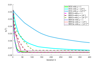
(a) iteration v.s. objective function value

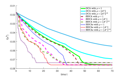
(b) time v.s. objective function value

Figure 2: The behaviors of DCA, BDCA and BDCA_e with different strong convexity modulus $\rho\in\{1,\|\mathbf{A}^{+}\|,\|\mathbf{A}^{+}\|^{1.5}\}$ for a problem of $45$ assets using a random initial point.

In Table 2, we report the numerical results comparing BDCA${}_{\text{e}}$ with DCA, BDCA on objective function values, the CPU time (in seconds), and the iterations for (T–P${}_{\text{dc}}$) and (HD–P${}_{\text{dc}}$), as well as the solvers FILTERSD and FMINCON on objective values and the CPU time. We choose the modulus $\rho=1$ for DCA and $\rho=\|A^{+}\|$ for BDCA and BDCA${}_{\text{e}}$ based on Fig. 2. The average CPU time and the average iterations are also reported. On average CPU time, we observe that BDCA${}_{\text{e}}$ is the fastest method among the others for both (T–P${}_{\text{dc}}$) and (HD–P${}_{\text{dc}}$). Concerning the objective values, we observe that DCA and FILTERSD provide the best objective values in all tested examples. Our BDCA${}_{\text{e}}$ for both (T–P${}_{\text{dc}}$) and (HD–P${}_{\text{dc}}$) shares the same function values in most of cases except for instances of No. $11,14,17,20,23$, and the differences in the objective values between BDCA${}_{\text{e}}$ and DCA as well as FILTERSD in these instances are within $O(10^{-5})$. Besides, we can see that BDCA${}_{\text{e}}$ for (HD–P${}_{\text{dc}}$) is about 1.5 times faster than BDCA and FMINCON, 2 times faster than FILTERSD, and more than 3 times faster than DCA on average CPU time. In conclusion, BDCA${}_{\text{e}}$ outperforms the other compared methods on (HD–P${}_{\text{dc}}$).

Table 2: Numerical results of DCA with $\rho=1$, BDCA and BDCA${}_{\text{e}}$ with $\rho=\|A^{+}\|$ for problem (T–P${}_{\text{dc}}$) and (HD–P${}_{\text{dc}}$) as well as FILTERSD and FMINCON with default parameters; bold values for best results in objective function.

No.	$n$	Algorithms for solving (T–P${}_{\text{dc}}$)									Algorithms for solving (HD–P${}_{\text{dc}}$)									FILTERSD		FMINCON
		DCA			BDCA			BDCA${}_{\text{e}}$			DCA			BDCA			BDCA${}_{\text{e}}$
		iter	time	obj	iter	time	obj	iter	time	obj	iter	time	obj	iter	time	obj	iter	time	obj	time	obj	time	obj
1	11	1213	3.95	-9.675e-02	27	0.17	-9.675e-02	12	0.08	-9.675e-02	1232	1.54	-9.675e-02	26	0.08	-9.675e-02	11	0.04	-9.675e-02	0.03	-9.675e-02	0.09	-9.675e-02
2	11	505	2.34	5.625e-03	54	0.41	5.625e-03	13	0.08	5.625e-03	504	0.86	5.625e-03	48	0.13	5.625e-03	21	0.05	5.625e-03	0.03	5.625e-03	0.10	5.627e-03
3	11	305	1.43	-9.993e-02	72	1.14	-9.993e-02	17	0.11	-9.993e-02	326	0.54	-9.993e-02	50	0.17	-9.993e-02	28	0.06	-9.993e-02	0.08	-9.993e-02	0.17	-9.993e-02
4	16	225	4.10	-1.522e-01	34	0.57	-1.522e-01	15	0.27	-1.522e-01	244	4.11	-1.522e-01	33	0.40	-1.522e-01	17	0.23	-1.522e-01	0.14	-1.522e-01	0.32	-1.522e-01
5	16	486	6.19	8.175e-03	67	1.12	8.175e-03	29	0.42	8.175e-03	434	2.46	8.175e-03	51	0.49	8.175e-03	33	0.39	8.175e-03	0.19	8.175e-03	0.37	8.179e-03
6	16	396	4.39	-8.260e-02	45	0.72	-8.260e-02	21	0.35	-8.260e-02	403	2.38	-8.260e-02	43	0.35	-8.260e-02	20	0.20	-8.260e-02	0.15	-8.260e-02	0.32	-8.259e-02
7	21	179	8.61	-1.647e-01	44	3.26	-1.647e-01	22	1.35	-1.647e-01	189	11.42	-1.647e-01	43	1.82	-1.647e-01	22	1.03	-1.647e-01	0.79	-1.647e-01	0.68	-1.647e-01
8	21	477	18.77	1.574e-03	88	8.51	1.574e-03	21	1.18	1.574e-03	444	7.29	1.574e-03	54	1.39	1.574e-03	22	0.65	1.574e-03	0.81	1.574e-03	1.58	1.579e-03
9	21	308	12.16	-9.945e-02	240	16.56	-9.945e-02	37	2.12	-9.945e-02	313	8.08	-9.945e-02	82	3.51	-9.945e-02	25	1.03	-9.945e-02	0.98	-9.945e-02	1.18	-9.945e-02
10	26	138	15.34	-1.302e-01	56	5.26	-1.302e-01	27	2.98	-1.302e-01	224	13.94	-1.302e-01	56	3.56	-1.302e-01	28	2.16	-1.302e-01	2.33	-1.302e-01	2.20	-1.302e-01
11	26	472	31.45	4.184e-03	68	10.16	4.185e-03	30	3.61	4.185e-03	457	16.84	4.184e-03	68	3.25	4.185e-03	28	1.42	4.185e-03	3.28	4.184e-03	4.52	4.191e-03
12	26	349	19.52	-1.077e-01	102	11.10	-1.077e-01	30	3.11	-1.077e-01	373	13.97	-1.077e-01	92	5.74	-1.077e-01	32	2.30	-1.077e-01	2.46	-1.077e-01	3.08	-1.077e-01
13	31	107	15.73	-1.649e-01	58	9.59	-1.649e-01	32	11.18	-1.649e-01	166	19.45	-1.649e-01	58	7.74	-1.649e-01	31	5.04	-1.649e-01	6.16	-1.649e-01	4.31	-1.649e-01
14	31	565	65.38	9.530e-04	77	12.52	9.543e-04	54	9.50	9.543e-04	545	29.18	9.530e-04	109	8.15	9.555e-04	46	3.86	9.566e-04	6.51	9.530e-04	9.18	9.613e-04
15	31	513	55.87	-1.082e-01	129	37.56	-1.082e-01	37	6.86	-1.082e-01	535	30.66	-1.082e-01	86	9.68	-1.082e-01	42	4.87	-1.082e-01	7.46	-1.082e-01	7.75	-1.082e-01
16	36	67	21.60	-1.649e-01	64	18.56	-1.649e-01	35	12.26	-1.649e-01	106	24.12	-1.649e-01	66	15.51	-1.649e-01	33	9.76	-1.649e-01	14.61	-1.649e-01	9.00	-1.649e-01
17	36	597	128.97	7.728e-04	85	26.76	7.769e-04	67	22.47	7.764e-04	591	53.18	7.728e-04	82	8.71	7.769e-04	34	4.29	7.740e-04	14.75	7.732e-04	20.67	7.824e-04
18	36	320	55.33	-1.144e-01	85	22.47	-1.144e-01	39	12.35	-1.144e-01	336	37.12	-1.144e-01	90	16.96	-1.144e-01	47	13.85	-1.144e-01	15.84	-1.144e-01	15.95	-1.144e-01
19	41	71	28.43	-1.650e-01	75	33.74	-1.650e-01	41	23.08	-1.650e-01	87	28.83	-1.650e-01	73	21.74	-1.650e-01	40	14.84	-1.650e-01	28.47	-1.650e-01	15.81	-1.650e-01
20	41	599	217.92	8.431e-04	117	51.56	8.436e-04	59	28.40	8.456e-04	592	81.15	8.431e-04	112	23.45	8.452e-04	75	18.25	8.484e-04	28.58	8.431e-04	34.87	8.540e-04
21	41	223	61.09	-1.083e-01	88	35.27	-1.083e-01	40	20.14	-1.083e-01	238	41.35	-1.083e-01	93	25.09	-1.083e-01	44	16.36	-1.083e-01	28.22	-1.083e-01	21.93	-1.083e-01
22	46	65	34.28	-1.650e-01	77	51.42	-1.650e-01	43	33.65	-1.650e-01	71	25.71	-1.650e-01	77	31.35	-1.650e-01	44	22.85	-1.650e-01	60.59	-1.650e-01	29.71	-1.650e-01
23	46	483	276.73	1.165e-03	111	78.71	1.168e-03	67	53.35	1.166e-03	474	104.54	1.165e-03	111	34.76	1.168e-03	72	26.76	1.165e-03	67.20	1.165e-03	74.03	1.177e-03
24	46	324	139.86	-1.146e-01	102	61.48	-1.146e-01	49	53.01	-1.146e-01	336	87.68	-1.146e-01	106	53.20	-1.146e-01	49	36.87	-1.146e-01	64.49	-1.146e-01	48.95	-1.146e-01
average		374	51.23		82	20.78		35	12.58		384	26.93		71	11.55		35	7.80		14.76		12.78

Fig. 3 demonstrates the $\log$ average CPU time for the instances in Table 2 along the number of assets $n$. We observe that DCA for (T–P${}_{\text{dc}}$) has the worst performance, while FILTERSD has the best performance when $n$ is less than about $22$. As $n$ increases beyond $22$, the best result is given by BDCA${}_{\text{e}}$ for (HD–P${}_{\text{dc}}$), and the methods BDCA for (HD–P${}_{\text{dc}}$), BDCA${}_{\text{e}}$ for (T–P${}_{\text{dc}}$), FMINCON, and FILTERSD have almost the same performance, which demonstrates that BDCA${}_{\text{e}}$ should be a promising approach to outperform the others on large-scale settings.

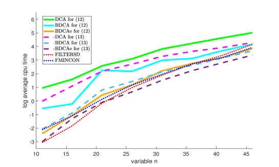
Figure 3: Plot the curve for $\log$ average CPU time of the data generated in Table 2 for each $n$ of DCA, BDCA and BDCA${}_{\text{e}}$ for (T–P${}_{\text{dc}}$) and (HD–P${}_{\text{dc}}$) as well as FILTERSD and FMINCON. We choose the modulus $\rho=1$ for DCA and $\rho=\|A^{+}\|$ for BDCA and BDCA${}_{\text{e}}$.

8 Conclusions

In this paper, we presented a novel DC-SOS decomposition technique based on the power-sum representation for polynomials. We proposed an accelerated DCA (BDCA${}_{\text{e}}$) combining DCA with an exact line search along the DC descent direction for solving linearly constrained polynomial optimization problems. We proved that any limit point of the sequence $\{\mathbf{x}^{k}\}$ generated by BDCA${}_{\text{e}}$ is a critical point of (POPL) and established the convergence rate of the sequence $\{f(\mathbf{x}^{k})\}$ under the Kurdyka-Łojasiewicz assumption. We applied the FDPG method by exploiting the power-sum-DC structure for solving effectively the convex subproblems. The numerical experiments on the (MVSK) model indicated that BDCA${}_{\text{e}}$ outperformed BDCA with Armijo line search and DCA, as well as the solvers FILTERSD and FMINCON on average CPU time and almost always got the best objective values. In the future, one important question is to investigate a better way to generate power-sum-DC decompositions with a shorter basis or to generate a sparse power-sum-DC decomposition. Another important question is how to find an adaptive way to update strongly convex parameter $\rho$ for ensuring both acceleration and good computed solution. Moreover, taking advantage of the power-sum structure to more effectively solve convex subproblems is always an important research topic.

- (1) Ahmadi, A.A., Hall, G.: DC decomposition of nonconvex polynomials with algebraic techniques. Mathematical Programming 169(1), 69–94 (2018)
- (2) Ahmadi, A.A., Parrilo, P.A.: A convex polynomial that is not sos-convex. Mathematical Programming 135(1), 275–292 (2012)
- (3) Ahmadi, A.A., Parrilo, P.A.: A complete characterization of the gap between convexity and sos-convexity. SIAM Journal on Optimization 23(2), 811–833 (2013)
- (4) Artacho, F.J.A., Fleming, R.M., Vuong, P.T.: Accelerating the dc algorithm for smooth functions. Mathematical Programming 169(1), 95–118 (2018)
- (5) Artacho, F.J.A., Goberna, M.A., López, M.A., Rodríguez, M.M.: Nonlinear optimization. Springer (2019)
- (6) Artacho, F.J.A., Vuong, P.T.: The boosted dc algorithm for nonsmooth functions. SIAM J. Optim. 30(1), 980–1006 (2020)
- (7) Bakonyi, M., Johnson, C.R.: The euclidian distance matrix completion problem. SIAM Journal on Matrix Analysis and Applications 16(2), 646–654 (1995)
- (8) Beck, A.: First-order methods in optimization. SIAM (2017)
- (9) Blekherman, G.: Typical real ranks of binary forms. Foundations of Computational Mathematics 15(3), 793–798 (2015)
- (10) Bolte, J., Daniilidis, A., Lewis, A.: The łojasiewicz inequality for nonsmooth subanalytic functions with applications to subgradient dynamical systems. SIAM Journal on Optimization 17(4), 1205–1223 (2007)
- (11) Bomze, I.M., Locatelli, M.: Undominated dc decompositions of quadratic functions and applications to branch-and-bound approaches. Computational Optimization and Applications 28(2), 227–245 (2004)
- (12) Boyd, S., El Ghaoui, L., Feron, E., Balakrishnan, V.: Linear matrix inequalities in system and control theory. SIAM (1994)
- (13) Brás, C., Eichfelder, G., Júdice, J.: Copositivity tests based on the linear complementarity problem. Computational Optimization and Applications 63(2), 461–493 (2016)
- (14) Buczyńska, W., Buczyński, J., Teitler, Z.: Waring decompositions of monomials. Journal of Algebra 378, 45–57 (2013)
- (15) Burer, S.: On the copositive representation of binary and continuous nonconvex quadratic programs. Mathematical Programming 120(2), 479–495 (2009)
- (16) Carlini, E., Catalisano, M.V., Geramita, A.V.: The solution to the waring problem for monomials and the sum of coprime monomials. Journal of algebra 370, 5–14 (2012)
- (17) Chambadal, L.: Algèbre linéaire et algèbre tensorielle (2017)
- (18) Dür, M., Hiriart-Urruty, J.B.: Testing copositivity with the help of difference-of-convex optimization. Mathematical Programming 140(1), 31–43 (2013)
- (19) Fletcher, R.: Filtersd–a library for nonlinear optimization written in fortran (2015). URL https://projects.coin-or.org/filterSD
- (20) Frankel, P., Garrigos, G., Peypouquet, J.: Splitting methods with variable metric for Kurdyka–Łojasiewicz functions and general convergence rates. Journal of Optimization Theory and Applications 165(3), 874–900 (2015)
- (21) Gotoh, J., Takeda, A., Tono, K.: DC formulations and algorithms for sparse optimization problems. Mathematical Programming 169(1), 141–176 (2018)
- (22) Hartman, P.: On functions representable as a difference of convex functions. Pacific Journal of Mathematics 9(3), 707–713 (1959)
- (23) Hiriart-Urruty, J.B.: Generalized differentiability/duality and optimization for problems dealing with differences of convex functions. In: Convexity and duality in optimization, pp. 37–70. Springer (1985)
- (24) Kurdyka, K., Parusinski, A.: wf-stratification of subanalytic functions and the lojasiewicz inequality. Comptes rendus de l’Académie des sciences. Série 1, Mathématique 318(2), 129–133 (1994)
- (25) Le Thi, H.A.: An efficient algorithm for globally minimizing a quadratic function under convex quadratic constraints. Mathematical programming 87, 401–426 (2000)
- (26) Le Thi, H.A., Moeini, M., Pham, D.T., Judice, J.: A dc programming approach for solving the symmetric eigenvalue complementarity problem. Computational Optimization and Applications 51(3), 1097–1117 (2012)
- (27) Le Thi, H.A., Pham, D.T.: Solving a class of linearly constrained indefinite quadratic problems by DC algorithms. Journal of global optimization 11(3), 253–285 (1997)
- (28) Le Thi, H.A., Pham, D.T.: The DC (difference of convex functions) programming and DCA revisited with DC models of real world nonconvex optimization problems. Annals of operations research 133(1), 23–46 (2005)
- (29) Le Thi, H.A., Pham, D.T.: DC programming and DCA: thirty years of developments. Mathematical Programming 169(1), 5–68 (2018)
- (30) Łojasiewicz, S.: Ensembles semi-analytiques, institut des hautes etudes sci. Bures-sur-Yvette, France (1964)
- (31) Łojasiewicz, S.: Sur la géométrie semi et sous-analytique. In: Annales de l’institut Fourier, vol. 43, pp. 1575–1595 (1993)
- (32) Maringer, D., Parpas, P.: Global optimization of higher order moments in portfolio selection. Journal of Global optimization 43(2), 219–230 (2009)
- (33) Mella, M.: Base loci of linear systems and the waring problem. Proceedings of the American Mathematical Society 137(1), 91–98 (2009)
- (34) Nesterov, Y.E.: A method for solving the convex programming problem with convergence rate . In: Dokl. akad. nauk Sssr, vol. 269, pp. 543–547 (1983)
- (35) Niu, Y.S.: On difference-of-sos and difference-of-convex-sos decompositions for polynomials. arXiv :1803.09900 (2018)
- (36) Niu, Y.S., Glowinski, R.: Discrete dynamical system approaches for boolean polynomial optimization. to appear in Journal of Scientific Computing, arXiv preprint arXiv:1912.10221 (2019)
- (37) Niu, Y.S., Júdice, J., Le Thi, H.A., Pham, D.T.: Solving the quadratic eigenvalue complementarity problem by dc programming. In: Modelling, Computation and Optimization in Information Systems and Management Sciences, pp. 203–214. Springer (2015)
- (38) Niu, Y.S., Júdice, J., Le Thi, H.A., Pham, D.T.: Improved dc programming approaches for solving the quadratic eigenvalue complementarity problem. Applied Mathematics and Computation 353, 95–113 (2019)
- (39) Niu, Y.S., Pham, D.T.: DC programming approaches for bmi and qmi feasibility problems. In: Advanced Computational Methods for Knowledge Engineering, pp. 37–63. Springer (2014)
- (40) Niu, Y.S., Pham, D.T., Le Thi, H.A., Júdice, J.: Efficient dc programming approaches for the asymmetric eigenvalue complementarity problem. Optimization Methods and Software 28(4), 812–829 (2013)
- (41) Niu, Y.S., Wang, Y.J., Le Thi, H.A., Pham, D.T.: Higher-order moment portfolio optimization via an accelerated difference-of-convex programming approach and sums-of-squares. arXiv :1906.01509 (2019)
- (42) Niu, Y.S., Zhang, H.: Power-product matrix: nonsingularity, sparsity and determinant. arXiv:2104.05209 (2021)
- (43) de Oliveira, W., Tcheou, M.P.: An inertial algorithm for dc programming. Set-Valued and Variational Analysis 27(4), 895–919 (2019)
- (44) Pham, D.T., Le Thi, H.A.: Convex analysis approach to DC programming: theory, algorithms and applications. Acta mathematica vietnamica 22(1), 289–355 (1997)
- (45) Pham, D.T., Le Thi, H.A.: A DC optimization algorithm for solving the trust-region subproblem. SIAM Journal on Optimization 8(2), 476–505 (1998)
- (46) Pham, D.T., Le Thi, H.A., Pham, V.N., Niu, Y.S.: DC programming approaches for discrete portfolio optimization under concave transaction costs. Optimization letters 10(2), 261–282 (2016)
- (47) Pham, D.T., Niu, Y.S.: An efficient dc programming approach for portfolio decision with higher moments. Computational Optimization and Applications 50(3), 525–554 (2011)
- (48) Pham, D.T., Souad, E.B.: Duality in dc (difference of convex functions) optimization. subgradient methods. Trends in mathematical optimization pp. 277–293 (1988)
- (49) Phan, D.N., Le, H.M., Le Thi, H.A.: Accelerated difference of convex functions algorithm and its application to sparse binary logistic regression. In: IJCAI, pp. 1369–1375 (2018)
- (50) Polyak, B.T.: Some methods of speeding up the convergence of iteration methods. Ussr computational mathematics and mathematical physics 4(5), 1–17 (1964)
- (51) Shelton, R., Heuvers, K.J., Moak, D., Rao, K.B.: Multinomial matrices. Discrete mathematics 61(1), 107–114 (1986)
- (52) Song, Y., Yu, G.: Properties of solution set of tensor complementarity problem. Journal of Optimization Theory and Applications 170(1), 85–96 (2016)
- (53) Wen, B., Chen, X., Pong, T.K.: A proximal difference-of-convex algorithm with extrapolation. Computational optimization and applications 69(2), 297–324 (2018)
- (54) You, Y., Niu, Y.S.: A refined inertial dc algorithm for dc programming. Optimization and Engineering pp. 1–27 (2022)