The tropological vertex

School of Mathematics, Monash University, VIC 3800 Australia
Email: norm.do@monash.edu

Mathematical Sciences Institute, The Australian National University, ACT 2601 Australia
Email: brett.parker@anu.edu.au

Abstract. The theory of the topological vertex was originally proposed by Aganagic, Klemm, Mariño and Vafa as a means to calculate open Gromov–Witten invariants of toric Calabi–Yau threefolds. In this paper, we place the topological vertex within the context of relative Gromov–Witten invariants of log Calabi–Yau manifolds and describe how these invariants can be effectively computed via a gluing formula for the enumeration of tropical curves in a singular integral affine space. This richer context allows us to prove that the topological vertex possesses certain tropical symmetries. These symmetries are captured by the action of a quantum torus Lie algebra that is related to a quantisation of the Lie algebra of the tropical vertex group of Gross, Pandharipande and Siebert. Finally, we demonstrate how this algebra of symmetries leads to an explicit description of the topological vertex and related Gromov–Witten invariants.

Keywords. Gromov–Witten invariants, topological vertex, tropical geometry

2020 Mathematics Subject Classification. 14N35, 53D45

Acknowledgements. The first author was supported by the Australian Research Council grant DP180103891. Both authors thank the mathematical research institute MATRIX in Australia where part of this research was performed. Both authors thank Jean-Emile Bourgine for directing us to reference [3].

 

 

1 Introduction

Aganagic, Klemm, Mariño and Vafa introduced the theory of the topological vertex for the effective computation of open Gromov–Witten invariants, motivated by the duality between Chern–Simons theory and Gromov–Witten theory [2, 9]. Li, Liu, Liu and Zhou provided a rigorous mathematical construction of the topological vertex in terms of formal relative Gromov–Witten invariants [16]. We will relate this construction to Gromov–Witten invariants of three-dimensional log Calabi–Yau manifolds, which are computable using a calculus of tropical curves. This perspective provides an algebra of tropical symmetries of the topological vertex; hence, ‘the tropological vertex’.

The aforementioned tropical symmetries arise as a representation of a quantum torus Lie algebra, which is introduced in Section 13 and comes in two forms. The small quantum torus Lie algebra $\mathfrak{t}_{s}$ has generators $T_{(a,b)}$ for $(a,b)\in\mathbb{Z}^{2}\setminus\{(0,0)\}$ that satisfy the commutation relations

$$[T_{(a,b)},T_{(c,d)}]=[ad-bc]_{q}\,T_{(a+c,b+d)}\ ,$$

where we use the slightly unconventional notation $[n]_{q}:=-i(q^{n/2}-q^{-n/2})=2\sin(n\hbar/2)$ and the relation $q^{1/2}=e^{i\hbar/2}$. This small quantum torus Lie algebra is associated to a real 2-dimensional torus with Lie algebra $\mathfrak{t}^{2}$ so that the $\mathbb{Z}^{2}$ used to index the generators corresponds naturally to the integral lattice $\mathbb{Z}^{2}=\mathfrak{t}^{2}_{\mathbb{Z}}\subset\mathfrak{t}^{2}$. The big quantum torus Lie algebra $\mathfrak{t}_{b}$ is a central extension of $\mathfrak{t}_{s}$ by $\mathfrak{t}^{2}$, with generators that satisfy the commutation relations

$$[T_{(a,b)},T_{(c,d)}]=[ad-bc]_{q}\,T_{(a+c,b+d)}+\delta_{(a+c,b+d),(0,0)}(a,b)\ .$$

Our quantum torus Lie algebra can be regarded as a quantisation of the Lie algebra of the tropical vertex group of Gross, Pandharipande and Siebert [10], and also appears as the Lie algebra of the quantum tropical vertex group of Bousseau [5].

The main output of our analysis is the following, which appears subsequently with proof as 15.1.

Theorem.

For any $v\in\mathfrak{t}^{2}_{\mathbb{Z}}$, we have

$$\left(\mathcal{W}_{v,1^{-}}+\mathcal{W}_{v,2^{-}}+\mathcal{W}_{v,3^{-}}\right)\mathfrak{T}=0\ .$$

One can think of $\mathfrak{T}$ as a partition function for the topological vertex, storing certain Gromov–Witten invariants of $\mathbb{C}^{3}$, whose toric graph comprises three legs adjacent to a single vertex. The operators $\mathcal{W}_{v,\ell}$ encode Gromov–Witten invariants that virtually count holomorphic curves with an extra constraint corresponding to $v\in\mathfrak{t}^{2}_{\mathbb{Z}}$ on the leg $\ell$ of the toric graph. Using a calculus of tropical curves, we prove that the map

$$T_{v}\longmapsto\mathcal{W}_{v,1^{-}}+\mathcal{W}_{v,2^{-}}+\mathcal{W}_{v,3^{-}}$$

produces a representation of the small quantum torus Lie algebra $\mathfrak{t}_{s}$. Thus, the result above demonstrates that tropical symmetries of the topological vertex are captured by the action of a quantum torus Lie algebra. A connection between the closely related quantum $\mathcal{W}_{1+\infty}$ algebra and the refined topological vertex was shown in the algebraic approach of Awata, Feigin and Shiraishi [3].

The relevant definitions and full details required for the statement and proof of the theorem above appear in the remainder of the paper.

The geometric setup for our analysis and results appears in Sections 2, 3 and 4.

• In Section 2, we discuss how to construct log Calabi–Yau manifolds from toric Calabi–Yau manifolds and relate the topological vertex to Gromov–Witten invariants of these log Calabi–Yau manifolds. The Lie algebra $\mathfrak{t}^{2}$ described above makes its first appearance here as an algebra of symmetries for such manifolds.

• In Section 3, we describe how holomorphic curves in these log Calabi–Yau manifolds can be studied via tropical curves in a singular integral affine space.

• In Section 4, we introduce the spaces used to encode Gromov–Witten invariants of these log Calabi–Yau manifolds. In this three-dimensional Calabi–Yau setting, it turns out that these evaluation spaces have a holomorphic symplectic structure and the image of the moduli space of holomorphic curves is holomorphic Lagrangian.

The algebraic setup for our analysis and results appears in Sections 5, 6, 7 and 8.

• In Sections 5 and 6, we explain how to encode Gromov–Witten invariants using cohomology classes and package them in suitable generating functions. We then introduce a Novikov ring $\mathfrak{N}$ in which such generating functions naturally reside, which allows us to keep track of the symplectic area and Euler characteristic of the curves that we enumerate.

• In Sections 7 and 8, we package the possible constraints for the Gromov–Witten invariants of interest into an algebra $\mathcal{H}$, which plays the role of a bosonic Fock space of quantum states. We encode the full Gromov–Witten theory in a partition function $\exp\eta\in\mathcal{H}$ that can be determined tropically, but contains more information than the topological vertex. The topological vertex partition function $Z_{\bar{X}}$ is obtained by projecting $\mathcal{H}$ to a subalgebra $\mathcal{H}^{\pm}$, corresponding to counting holomorphic curves with particular constraints. This constrained state space $\mathcal{H}^{\pm}$ is naturally a tensor product of algebras $\mathcal{H}^{\pm}_{\ell}$ over the legs $\ell$ of the toric graph associated to our toric Calabi–Yau manifold.

The analysis that leads to a proof of our main result appears in the remaining Sections 9, 11, 10, 12, 13, 14 and 15.

• In Section 9, we reformulate the gluing formula for topological vertex partition functions in the language of this paper. This formula can be derived from the tropical gluing formula appearing in previous work of the second author [23, Equation (1)]. We briefly present this tropical gluing formula, which is also required for subsequent arguments in the paper.

• In Sections 11 and 10, we calculate Gromov–Witten invariants in the simplest cases by using the tropical correspondence formula for three-dimensional toric manifolds as a key input [22]. This allows us to give a complete analysis of the cases $X=\mathbb{C}\times(\mathbb{C}^{*})^{2}$ and $X=\mathbb{C}^{2}\times\mathbb{C}^{*}$, which correspond to the empty tropical graph and the tropical graph with no vertices, respectively.

• In Sections 12 and 13, we construct operators $\mathcal{W}_{v,\ell}$ on $\mathcal{H}_{\ell}^{+}$ that encode Gromov–Witten invariants counting holomorphic curves with an extra constraint corresponding to $v\in\mathfrak{t}^{2}_{\mathbb{Z}}\setminus\{0\}$. 12.3 states that these operators provide a representation of the big quantum torus Lie algebra $\mathfrak{t}_{b}$, corresponding to a projective representation of $\mathfrak{t}_{s}$. The proof involves the calculus of tropical curves, using diagrams such as that pictured in Figure 1. It also relies heavily on the aforementioned tropical gluing formula and three-dimensional tropical correspondence formula of the second author [23, 22]. We then prove that this is a highest weight representation with weights calculated in Lemmas 12.4 and 12.5.

  Figure 1: $\mathcal{W}_{v,\ell}\mathcal{W}_{w,\ell}=\mathcal{W}_{w,\ell}\mathcal{W}_{v,\ell}+\left[{v\wedge w}\right]_{q}\,\mathcal{W}_{v+w,\ell}$

• In Section 14, we analyse the behaviour of the operators $\mathcal{W}_{v,\ell}$ under a change of framing. Recall that a choice of framing is required for each leg $\ell$ in order to define the topological vertex. We prove that the structure of $\mathcal{H}^{+}_{\ell}$ as a highest weight representation does not depend on the framing, so the framing change isomorphism $F_{\bar{X}}$ is an isomorphism of representations. Again, the proof involves the calculus of tropical curves, using diagrams such as that pictured in Figure 2.

  Figure 2: $F_{\bar{X}}\circ\mathcal{W}_{v,\ell_{1}}=\mathcal{W}_{v,\ell_{2}^{-}}\circ F_{\bar{X}}$.

• In Section 15, we consider the topological vertex partition function, corresponding to the toric Calabi–Yau manifold $X=\mathbb{C}^{3}$, whose toric graph comprises three legs adjacent to a single vertex. The partition function $Z_{\bar{X}}$ is an element of the algebra $\mathcal{H}^{+}_{1^{-}}\otimes\mathcal{H}^{+}_{2^{-}}\otimes\mathcal{H}^{+}_{3^{-}}$, which has a representation of the small quantum torus Lie algebra $\mathfrak{t}_{s}$ induced from the representations of $\mathfrak{t}_{b}$ on the three tensor factors. We state and prove our main results — 15.1 and 15.2 — which assert that $Z_{\bar{X}}$ is invariant under this action, thereby giving rise to tropical symmetries of the topological vertex. Once again, the proof involves the calculus of tropical curves, using diagrams such as that pictured in Figure 3. We conclude the paper by showing how these symmetries allow one to effectively calculate the topological vertex in Lemmas 15.3, 15.4 and 15.5 and 15.6.

  Figure 3: Two ways of calculating a Gromov–Witten invariant to derive tropical symmetries of the topological vertex.

Our general approach relies on the theory of exploded manifolds developed by the second author in a series of previous works [21, 22, 23, 24, 25, 26]. However, our main results only depend largely on two main outputs of that program — the tropical gluing formula and the three-dimensional tropical correspondence formula.

In separate work, we give an independent proof of our tropical symmetries using the operator formalism on the infinite wedge space and discuss consequences for the integrability of topological vertex partition functions [7]. In that context, we observe that the $W$ operators introduced in this paper agree with the $\mathcal{E}$ operators that arise in the Gromov–Witten/Hurwitz correspondence of Okounkov and Pandharipande [20].

2 From toric Calabi–Yau to log Calabi–Yau

A toric Calabi–Yau threefold $X$ is a (non-compact) toric manifold with $\dim_{\mathbb{C}}X=3$ and a holomorphic volume form $\Omega$. In toric coordinates,

$$\Omega_{X}=f\frac{\mathrm{d}z_{1}}{2\pi iz_{1}}\wedge\frac{\mathrm{d}z_{2}}{2\pi iz_{2}}\wedge\frac{\mathrm{d}z_{3}}{2\pi iz_{3}}\ ,$$

where $f:X\longrightarrow\mathbb{C}$ is a globally defined holomorphic function, whose vanishing set is the toric boundary divisor of $X$. So on the interior of $X$, $\Omega_{X}$ is $f$ multiplied by the unique $(\mathbb{C}^{*})^{3}$–invariant holomorphic $3$-form with integral equal to 1 on each each torus fibre. Assume that the toric fan of $X$ is convex and that $f$ is a primitive monomial in the toric coordinates. Let $\bar{X}$ be a smooth toric compactification of $X$ such that $f$ extends to a meromorphic function on $\bar{X}$, and vanishes only on the toric boundary strata of $X\subset\bar{X}$. The form

$$\Omega_{\bar{X}}:=\frac{\Omega_{X}}{1-f}$$

extends to a meromorphic volume form on $\bar{X}$ with poles at the simple normal crossing divisor

$$D:=f^{-1}(1)\cup(\bar{X}\setminus X)$$

and $(\bar{X},D)$ is a log Calabi–Yau manifold with logarithmic holomorphic volume form $\Omega_{\bar{X}}$. We will study Gromov–Witten invariants of $\bar{X}$ relative to the simple normal crossing divisor $D$ and relate these to the topological vertex of Aganagic, Klemm, Mariño and Vafa [2].

2.1 Toric graphs

Let $\mathbb{T}^{2}$ be the sub-torus preserving $f$, and let $\mathfrak{t}^{2}$ be the corresponding Lie algebra. This has a canonical integral lattice, $\mathfrak{t}^{2}_{\mathbb{Z}}\subset\mathfrak{t}^{2}$ comprised of the elements whose time 1 flow is the identity. Choose a $\mathbb{T}^{2}$–invariant symplectic form $\omega$ on $\bar{X}$ defining a Kähler structure. This can be a toric symplectic form, however the following discussion does not require that $\omega$ be $\mathbb{T}^{3}$ invariant.

The moment map of the $\mathbb{T}^{2}$-action is a map

$$\pi:\bar{X}\longrightarrow(\mathfrak{t}^{2})^{*}=\mathbb{R}^{2}\ ,$$

defined up to translation by the condition that for $v\in\mathfrak{t}^{2}$ and $\widetilde{v}$ the corresponding vector field on $X$, $-i_{\widetilde{v}}\omega=\pi^{*}dv$, where we consider $v$ as giving a linear function on $(\mathfrak{t}^{2})^{*}$. Within $X\subset\bar{X}$, the $\mathbb{T}^{2}$-action is free away from toric boundary strata of codimension at least $2$; the image of these strata is a graph called the toric graph of $X$. The edges of this toric graph travel in integral directions: if the flow of $v\in\mathfrak{t}^{2}$ is constant on the stratum over an edge, then the linear function $v$ on $(\mathfrak{t}^{2})^{*}$ is constant on that edge. For an edge $e$, a choice of primitive integral generator $v_{e}\in\mathfrak{t}^{2}_{\mathbb{Z}}$ for the sub-torus preserving this stratum then corresponds to a choice of coorientation of $e$. Call such a $v_{e}$ a normal vector to the edge $e$. Vertices of this toric graph are trivalent, and with a cyclic choice of coorientation of the edges leaving a vertex, the corresponding normal vectors sum to $0$. Moreover, we can always choose $\mathbb{Z}$-affine coordinates $(x,y)$ centred on a vertex such that these cyclically oriented normal vectors are $(0,1)$, $(-1,0)$, and $(1,-1)$.

The edges of a toric graph can also end at the boundary of $\pi(\bar{X})$, which is a compact, convex polytope. Such an end is called a leg. In $\bar{X}$, this leg $\ell$ corresponds to a $0$-dimensional stratum of $\bar{X}$, the intersection of two codimension $1$ strata of $X$, and one extra codimension $1$ stratum $\bar{X}_{\ell}$ of $\bar{X}$. Our conditions on $\bar{X}$ ensure that this extra stratum is necessarily fixed by the flow of some primitive $w_{\ell}\in\mathfrak{t}^{2}_{\mathbb{Z}}$ such that the corresponding boundary face of the polytope $\pi(\bar{X})$ is where the linear function $w_{\ell}$ on $(\mathfrak{t}^{2})^{*}$ is constant and achieves its maximum. Moreover, $w_{\ell}$ and the normal vector to the edge form a basis for the lattice $\mathfrak{t}^{2}_{\mathbb{Z}}$, so there exist $\mathbb{Z}$-affine coordinates $(x,y)$ such that the edge is a positive ray in the $x$ direction, and $w_{\ell}=x$. Different choices of compactification $\bar{X}\supset X$ lead to different $w_{\ell}$, and a choice of such $w_{\ell}$ is called a $\bf{framing}$. See Figure 4 for an example of a toric graph.

Figure 4: A toric graph with four legs and framing vectors $(-1,0)$, $(-1,0)$, $(0,1)$, $(0,-1)$.

This stratum $\bar{X}_{\ell}\subset\bar{X}$ where the leg $\ell$ ends naturally has the structure of a $2$-dimensional log Calabi–Yau manifold. The divisor $D_{\ell}\subset\bar{X}_{\ell}$ is the intersection of $\bar{X}_{\ell}$ with the strata of $\bar{X}$ that don’t contain $\bar{X}_{\ell}$. To obtain the holomorphic volume form $\Omega_{\bar{X}_{\ell}}$ on $\bar{X}_{\ell}$, denote by $\iota_{w_{\ell}}\Omega_{\bar{X}}$ the holomorphic $2$–form on $\bar{X}$ obtained by inserting the vector field generating the flow of $w_{\ell}$; so if $z$ is a primitive monomial vanishing on $\bar{X}_{\ell}\subset\bar{X}$, then $\Omega_{\bar{X}}=-\frac{\mathrm{d}z}{2\pi iz}\wedge\iota_{w_{\ell}}\Omega_{\bar{X}}$. Then $\Omega_{\bar{X}_{\ell}}$ is the restriction of $\iota_{w_{\ell}}\Omega_{\bar{X}}$ to $\bar{X}_{\ell}\subset\bar{X}$. We will also think of $\Omega_{\bar{X}_{\ell}}$ as a holomorphic symplectic form on $(\bar{X}_{\ell},D_{\ell})$.

2.2 Lagrangian fibrations

The holomorphic map

$$f:\bar{X}\longrightarrow\mathbb{CP}^{1}$$

is a submersion away from $0$ and $\infty$, and the nondegenerate fibres are Kähler, with structure preserved by the $\mathbb{T}^{2}$-action. Parallel transport orthogonal to fibres defines a symplectic connection on this bundle. This connection preserves the symplectic structure, and also the $\mathbb{T}^{2}$-action and its moment map $\pi$. We can use this connection to define various Lagrangians in $X$ and $\bar{X}$. Because the moment map $\pi$ is preserved, parallel transport of a $\mathbb{T}^{2}$-orbit around any smooth closed curve $\gamma$ in $\mathbb{CP}^{1}\setminus\{0,\infty\}$ closes up to give a Lagrangian torus in $\bar{X}$. Moreover, this Lagrangian is $f^{-1}(\gamma)\cap\pi^{-1}(p)$ for some point $p\in(\mathfrak{t}^{2})^{*}$. For example, the $\mathbb{T}^{3}$-orbits are the parallel transport of $\mathbb{T}^{2}$-orbits around the loops where $\left\lvert f\right\rvert$ is constant. Parallel transport around the loops where $\left\lvert f-1\right\rvert$ is constant defines a nice singular Lagrangian torus fibration on $\bar{X}$ such that the behaviour of this fibration around the divisor $D\subset\bar{X}$ is like the behaviour of a toric fibration near the toric boundary divisor. Moreover, $\Omega_{\bar{X}}$ is purely real on these Lagrangian fibres, so this is a special Lagrangian fibration. The geometric significance of this is that, if $\omega$ defined a Kähler metric in which $\Omega_{\bar{X}}$ was covariantly constant, then these special Lagrangian fibres would have minimal volume, because their volume coincides with the integral of the closed form $\Omega_{\bar{X}}$. In $f^{-1}(0)$, there are singularities of this fibration where $\mathrm{d}f=0$, but as $\mathrm{d}f\neq 0$ away from codimension 2 strata of $X$, the fibration is smooth away from such strata. So we have singular Lagrangian torus fibration

$$(\ln\left\lvert f-1\right\rvert,\pi):\bar{X}\longrightarrow[-\infty,\infty]\times(\mathfrak{t}^{2})^{*}\ ,$$

which is smooth away from the embedding of the toric graph in $\{0\}\times(\mathfrak{t}^{2})^{*}$, which we will call the singular locus. We will also refer to the inverse image of this graph in $\bar{X}$ as the singular locus — this is actually a union of holomorphic spheres, one over each edge of the toric graph; it is also the locus where $f=0$ and $\mathrm{d}f=0$. Over any point in an edge of the singular locus, the fibre degenerates to an immersed Lagrangian $S^{1}\times S^{2}$ which intersects itself in a circle where $f=0$. These singular fibres degenerate further to have a more complicated singularity at $f=0$ over a vertex.

On the complement of the singular locus, the smooth Lagrangian torus fibration induces a $\mathbb{Z}$-affine structure on the base. This structure is such that if $(x_{1},x_{2},x_{3})$ are local $\mathbb{Z}$-affine coordinates on the base, they locally generate a free Hamiltonian $\mathbb{T}^{3}$-action on $\bar{X}$ with orbits the Lagrangian torus fibres. If $w\in\mathfrak{t}^{2}$ is integral, the corresponding linear function on $(\mathfrak{t}^{2})^{*}$ is a $\mathbb{Z}$-affine function, however there is monodromy in the $\mathbb{Z}$-affine structure around the singular locus, so there are not global $\mathbb{Z}$-affine coordinates. Note that the real part of $\Omega_{\bar{X}}$ gives an orientation form on fibres, and hence induces an orientation on the base — we choose the convention that if $(x_{1},x_{2},x_{3})$ are oriented $\mathbb{Z}$-affine coordinates, then the Hamiltonian vector fields generated by $-x_{1}$, $-x_{2}$ and $-x_{3}$ provide an oriented basis for the tangent space of the fibres.

This fibration also restricts to a singular special Lagrangian torus fibration on the toric boundary stratum $\bar{X}_{\ell}$ at the end of a leg $\ell$. Here, the singular locus consists of a single point. Both the $\mathbb{Z}$-affine stucture from the Lagrangian torus fibration and the orientation from $\Omega_{\bar{X}_{\ell}}$ coincide with the corresponding structure induced on the boundary of $\bar{X}$.

There is another interesting singular Lagrangian fibration

$$\left(\frac{f-1}{\left\lvert f-1\right\rvert},\pi\right):\bar{X}\setminus f^{-1}(\{1,\infty\})\longrightarrow S^{1}\times(\mathfrak{t}^{2})^{*}$$

whose fibres are now non-compact Lagrangian manifolds which are special in the sense that $\Omega_{\bar{X}}$ restricts to be purely imaginary on them. On $(X,\Omega_{X})$, there is a related non-compact special Lagrangian fibration given by the map $((f-\bar{f}),\pi)$. Of particular interest are the Aganagic–Vafa branes, given by $f^{-1}(-\infty,0]$ intersected with the inverse image of a point on an edge. These are diffeomorphic to $S^{1}\times\mathbb{R}^{2}$, intersecting $f^{-1}(0)$ in the circle $S^{1}\times\{0\}$; and are also special Lagrangians in $\bar{X}$ with the logarithmic holomorphic volume form $\Omega_{\bar{X}}$. These Aganagic–Vafa branes in $\bar{X}$ are non-compact, with their boundary a $\mathbb{T}^{2}$–orbit in $f^{-1}(\infty)$.

The above singular special Lagrangian fibration on $\bar{X}$ also restricts to $\bar{X}_{\ell}\subset\bar{X}$, and $\Omega_{\bar{X}_{\ell}}$ is also purely imaginary restricted to fibres. As there is a unique singular point corresponding to $\ell$ in the fibration of $\bar{X}_{\ell}$, there is a unique Aganagic–Vafa brane $A_{\ell}\subset\bar{X}_{\ell}$ corresponding to $\ell$ over $f^{-1}(-\infty,0]$. We orient $A_{\ell}$ so that $i\Omega_{\bar{X}_{\ell}}$ is a volume form on $A_{\ell}$. Topologically, $A_{\ell}\subset\bar{X}_{\ell}$ is a disk with boundary on $f^{-1}(\infty)$, so $A_{\ell}$ defines a class $[A_{\ell}]\in H_{2}(\bar{X}_{\ell},f^{-1}(\infty))$.

2.3 The topological vertex

The topological vertex, introduced by Aganagic, Klemm, Mariño and Vafa, involves a virtual count of holomorphic curves in $X=\mathbb{C}^{3}$ with boundary on three chosen Aganagic–Vafa branes over the three legs of the corresponding toric graph [2]. In this case, $f=z_{1}z_{2}z_{3}$ and the singular locus consists of the points where two coordinate functions vanish.

To define the topological vertex, the extra information of a framing is required — in [2], a framing is given by a choice of 1-dimensional sub-torus of $\mathbb{T}^{2}$ acting freely on this Aganagic–Vafa brane. Li, Liu, Liu, and Zhou provide a mathematical definition of the topological vertex using relative Gromov—Witten invariants [16]. In both [16] and our setting, the framing on each leg is provided by a toric compactification $\bar{X}$ of $X$, so the new boundary component $\bar{X}_{\ell}$ at the end of each leg $\ell$ is invariant under the 1-dimensional sub-torus given by the framing. Symplectically, this $\bar{X}_{\ell}$ can be regarded as the quotient of a hypersurface by this 1-dimensional sub-torus, and $A_{\ell}\subset\bar{X}_{\ell}$ is the quotient of an Aganagic–Vafa brane by this 1-dimensional sub-torus.

The definition of the topological vertex in [16] involves a count of holomorphic curves in $\bar{X}$, touching the new parts of the boundary divisor only in $A_{\ell}\subset\bar{X}_{\ell}$. Heuristically, a point on a holomorphic curve sent to $A_{\ell}$ and tangent to $\bar{X}_{\ell}$ with order $k$ plays the role of a boundary of a holomorphic curve that wraps $k$ times around the $S^{1}$ direction of the Aganagic–Vafa brane. In both [2] and [16], the invariants only see curves around the singular locus of $\bar{X}$, where $f=0$ and $\mathrm{d}f=0$. Accordingly, [16] defines the required curve counts in terms of formal relative Gromov–Witten invariants, with ‘formal’ meaning that the moduli stack of holomorphic curves is restricted to a formal neighbourhood of the curves in the singular locus. This restriction allows [16] to use the technology of Gromov–Witten invariants relative to smooth divisors from [15], avoiding the need for Gromov–Witten invariants relative to normal crossing divisors, which were only defined after [16] was published; see [11, 12, 25]. In what follows, we instead use Gromov–Witten invariants of $\bar{X}$ relative to the normal crossing divisor $D$, so that we can apply the tropical gluing formula from [23] to derive tropical symmetries of the topological vertex.

2.4 Substituting holomorphic constraints for Lagrangian constraints

In general, the moduli stack of holomorphic curves in $\bar{X}$ constrained using $A_{\ell}\subset\bar{X}_{\ell}$ has nonempty boundary, so it is more convenient for us to use different constraints. When no other legs have the same framing as $\ell$, $f^{-1}(0)\subset\bar{X}_{\ell}$ is the union of two embedded holomorphic spheres $E^{+}_{\ell}$ and $E^{-}_{\ell}$ so that

$$[E^{\pm}_{\ell}]=\pm[A_{\ell}]\text{ in }H_{2}(\bar{X}_{\ell},f^{-1}(\infty))\ .$$ (1)

We can make a minor perturbation of $A_{\ell}$ for different legs $\ell$, so that their image under $f$ intersects only at $0$. Then, the constraint of requiring holomorphic curves in $\bar{X}$ to only touch the divisor in these $A_{\ell}$ is satisfied only by curves in $f^{-1}(0)$. We can therefore get the same counts by using $E^{+}_{\ell}$ or $-E^{-}_{\ell}$ as a constraint in place of $A_{\ell}$.

Figure 5: A toric picture of $\bar{X}_{\ell}$, with divisor $D_{\ell}$ shown in yellow, the Lagrangian submanifold $A_{\ell}$ shown in green, and the holomorphic spheres $E^{+}_{\ell}$ shown in red, and $E^{-}_{\ell}$ shown in blue.

As classes in $H_{2}(\bar{X})$, we can readily calculate the intersections between $E^{\pm}_{\ell}$.

$$[E^{+}_{\ell}]\cdot[E^{-}_{\ell}]=1\qquad[E^{+}_{\ell}]\cdot[E^{+}_{\ell}]=-1\qquad[E^{-}_{\ell}]\cdot[E^{-}_{\ell}]=-1$$ (2)

These spheres $E^{\pm}_{\ell}$ are related to the two choices of normal vectors to the leg $\ell$. In particular, there is a canonical choice of normal vector $n_{\ell}\in\mathfrak{t}^{2}_{\mathbb{Z}}$ such that, for some choice of moment map, $\bar{X}\longrightarrow\mathfrak{(}\mathfrak{t}^{2})^{*}$ the hamiltonian function corresponding to $n_{\ell}$ is positive on $E^{+}$ and negative on $E^{-}$. Another way of describing this choice is as follows: removing their intersection with the divisor, $E^{\pm}$ is a complex plane, the action of $n_{\ell}$ on $E^{+}$ has weight $1$ and the action of $n_{\ell}$ on $E^{-}$ has weight $-1$.

When $k$ legs have the same framing, $f^{-1}(0)\subset\bar{X}_{\ell}$ consists of $k+1$ spheres. In this case define $E^{\pm}_{\ell}$ to be a union of these spheres satisfying equation 1. In each case, $f^{-1}(0)=E^{+}_{\ell}\cup E^{-}_{\ell}$, with both $E_{\ell}^{+}$ and $E^{-}_{\ell}$ connected, and intersecting only at the point in $\bar{X}_{\ell}$ corresponding to $\ell$. Equation 2 still holds. Moreover, for two legs $\ell$ and $\ell^{\prime}$ with the same framing, $[E^{\pm}_{\ell}]\cdot[E^{\pm}_{\ell^{\prime}}]=0$.

There exist toric degenerations of $X$ which break the original toric graph at some internal edges into matched pairs of legs $\ell^{+},\ell^{-}$ with the opposite framings $w_{\ell^{-}}=-w_{\ell^{+}}$. There is a natural identification of $\bar{X}_{\ell^{+}}$ with $\bar{X}_{\ell^{-}}$, but the induced holomorphic volume forms are opposite $\Omega_{\bar{X}_{\ell^{-}}}=-\Omega_{\bar{X}_{\ell^{+}}}$, so $E_{\ell^{-}}^{+}=E_{\ell^{+}}^{-}$. Holomorphic curves within $f^{-1}(0)$ in such situations can be analysed using tropical curves in a $\mathbb{Z}$-affine space modelled on $\mathfrak{t}^{2}$, but with a 1-dimensional piecewise linear singular locus. The broken internal edge of the toric graph corresponds to an edge in this singular locus travelling in the direction $w_{\ell^{+}}$, and there are tropical curves corresponding to $E_{\ell^{+}}^{\pm}$ travelling out from this singular edge in the directions $\pm n_{\ell^{+}}$. Our holomorphic volume form gives a canonical orientation of $\mathfrak{t}^{2}_{\mathbb{Z}}$ such that for each leg, $(w_{\ell},n_{\ell})$ is an oriented basis for $\mathfrak{t}^{2}_{\mathbb{Z}}$. See Figure 6 for an example of a toric degeneration.

Figure 6: A degeneration of $\bar{X}$ into four toric manifolds, and three red tropical curves ending on the black singular locus of the corresponding $\mathbb{Z}$-affine space.

Using Poincaré duals, we define the cohomology classes

$$\alpha_{\ell}=\alpha^{+}_{\ell}:=PD(E^{+}_{\ell})\qquad\text{and}\qquad\alpha^{-}_{\ell}:=PD(E^{-}_{\ell})\ .$$

Considering these cohomology classes as differential forms, we have

$$\int_{\bar{X}_{\ell}}\alpha^{+}_{\ell}\wedge\alpha^{-}_{\ell}=1\qquad\text{and}\qquad\int_{\bar{X}_{\ell}}\alpha^{\pm}_{\ell}\wedge\alpha^{\pm}_{\ell}=-1\ .$$

Inside the cohomology of $\bar{X}_{\ell}$ relative $f^{-1}(\infty)$, we have $\alpha^{-}_{\ell}=-\alpha^{+}_{\ell}$, and making this identification uncovers some beautiful structure in our Gromov–Witten invariants.

To explain the full structure of relative Gromov–Witten invariants of $(\bar{X},D)$, it is convenient to use exploded manifolds, so instead of the complex manifold $\bar{X}$ with the normal crossing divisor, we instead use its explosion $\operatorname{Expl}(\bar{X},D)$, and define invariants using exploded holomorphic curves in $\operatorname{Expl}(\bar{X},D)$; see [21, 26]. For the present discussion, it is enough to think of the moduli space of holomorphic curves in $\operatorname{Expl}(\bar{X},D)$ as a suitable compactification of the moduli space of holomorphic curves in $\bar{X}$, which are smooth and not contained in $D$. When we apply the explosion functor to such a smooth holomorphic curve, we obtain an exploded holomorphic curve in $\operatorname{Expl}(\bar{X},D)$, however the moduli space of exploded curves keeps track of more structure when such curves sink into the divisor. In particular, there is an evaluation map from the moduli stack of exploded curves analogous to the evaluation at a point of contact with $\bar{X}_{\ell}$, except now this map has codomain the exploded manifold $\operatorname{Expl}(\bar{X}_{\ell},D_{\ell})$. We introduce the notation

$$\mathbf{X}_{w_{\ell}}:=\operatorname{Expl}(\bar{X}_{\ell},D_{\ell})\ .$$

Evaluation at a point of contact order $k$ to $\bar{X}_{\ell}$ determines a map to the quotient stack $\bar{X}_{\ell}/\mathbb{Z}_{k}$, where we take the quotient by the trivial $\mathbb{Z}_{k}$-action. The exploded manifold analogue is given by

$$\mathbf{X}_{kw_{\ell}}/G_{kw_{\ell}},\quad\text{where }\mathbf{X}_{kw_{\ell}}:=\operatorname{Expl}(\bar{X}_{\ell},D_{\ell})\quad\text{and}\quad G_{kw_{\ell}}:=\mathbb{Z}_{k}\ .$$

As $E^{\pm}\longrightarrow\bar{X}_{\ell}$ is holomorphic, and not contained in $D_{\ell}$, we can apply the explosion functor to this map, and, using [24], define the Poincaré dual to this as the class $\alpha^{\pm}_{w_{\ell}}\in H^{2}(\mathbf{X}_{w_{\ell}})$. Pushing this class forward to $\mathbf{X}_{kw_{\ell}}/G_{kw_{\ell}}$ gives a class $\alpha^{\pm}_{k,\ell}\in H^{2}(\mathbf{X}_{kw_{\ell}}/G_{kw_{\ell}})$, whose pullback to $\mathbf{X}_{w_{\ell}}$ is $k\alpha^{\pm}_{\ell}$, and we have

$$\int_{\mathbf{X}_{kw_{\ell}}/G_{kw_{\ell}}}\alpha^{+}_{k,\ell}\wedge\alpha^{-}_{k,\ell}:=\frac{1}{k}\int_{\mathbf{X}_{w_{\ell}}}k\alpha^{+}_{\ell}\wedge k\alpha^{-}_{\ell}=k\qquad\text{and}\qquad\int_{\mathbf{X}_{kw_{\ell}}/G_{kw_{\ell}}}\alpha^{\pm}_{k,\ell}\wedge\alpha^{\pm}_{k,\ell}=-k.$$

3 Contact data and tropical curves

The exploded manifold $\operatorname{Expl}(\bar{X},D)$ has a functorial projection to a singular $\mathbb{Z}$-affine space, called its tropical part $\underline{\operatorname{Expl}(\bar{X},D)}$ [21]. This tropical part has a stratification into $\mathbb{Z}$-affine cones, each isomorphic to $[0,\infty)^{3}$, $[0,\infty)^{2}$, $[0,\infty)$, or a point, where each $k$-dimensional cone corresponds to the intersection of $k$ components of $D$. See Figure 7 for an example of the tropical part of an exploded manifold.

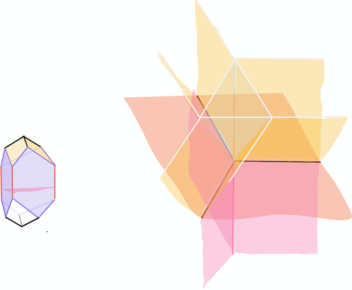
Figure 7: A toric moment polytope of $\bar{X}$ in the case $X=\mathbb{C}^{3}$ on the left and its tropical part $\underline{\operatorname{Expl}(\bar{X},D)}$ on the right.

In general, the $\mathbb{Z}$-affine structure on the tropical part of an exploded manifold does not extend across strata. In this case however, we can extend the $\mathbb{Z}$-affine structure to a global singular $\mathbb{Z}$-affine structure, with singular rays corresponding to the legs of our toric graph. Divide $\underline{\operatorname{Expl}(\bar{X},D)}$ into two nonsingular half spaces, glued over a wall isomorphic to $\mathfrak{t}^{2}$, to create a singular $\mathbb{Z}$-affine space with singularities along the rays spanned by framing vectors $w_{\ell}$. The top half of $\underline{\operatorname{Expl}(\bar{X},D)}$ is the tropical part of $\operatorname{Expl}(\bar{X},D)\setminus f^{-1}(1)$, which is naturally identified with the toric fan of $\bar{X}\setminus f^{-1}(0)$. As such, it has a natural global $\mathbb{Z}$-affine structure as a closed half space within the Lie algebra of the torus $\mathbb{T}^{3}$ acting on $\bar{X}$. The wall is the tropical part of $\operatorname{Expl}(\bar{X},D)\setminus f^{-1}(\{1,\infty\})$, which is naturally isomorphic to $\mathfrak{t}^{2}$, subdivided by the toric fan of $\bar{X}\setminus f^{-1}(\{0,\infty\})$. The bottom half is the tropical part of $\operatorname{Expl}(\bar{X},D)\setminus f^{-1}(\infty)$. This is naturally isomorphic to $\mathfrak{t}^{2}\times[0,\infty)$, with the stratification induced from the product of the stratification of the wall $\mathfrak{t}^{2}$, and $[0,\infty)$. The distinguished stratum $\{0\}\times[0,\infty)$ in this bottom half corresponds to the component $f^{-1}(1)$ of the divisor $D$.

We extend the $\mathbb{Z}$-affine structure of $\underline{\operatorname{Expl}(\bar{X},D)}$ by gluing the bottom half to the top half as follows. Let $v_{f}$ be the primitive integral vector in the $[0,\infty)$ direction, corresponding to the component $f^{-1}(1)$ of the divisor $D$. Using the given $\mathbb{Z}$-affine structure, we can transport $v_{f}$ anywhere in the bottom half, and we now specify how to transport $v_{f}$ into the top half over the interior of a 2-dimensional cone $\sigma$ on the wall. This cone corresponds to the intersection of two toric strata of $\bar{X}$ intersecting $f^{-1}(0)$ in exactly one stratum $S_{\sigma}$. Let $v_{S_{\sigma}}$ be the corresponding primitive integral vector in the toric fan of $\bar{X}$. This then can be considered as a constant vector field on the top half, which is naturally identified with half of the toric fan of $\bar{X}$. We extend the $\mathbb{Z}$-affine structure by gluing the top and bottom halves over $\sigma$ so $v_{f}$ is sent to $v_{S_{\sigma}}$ when we parallel transport $v_{f}$ over the cone $\sigma$. Note that this depends on the cone $\sigma$. If $\sigma$ and $\sigma^{\prime}$ intersect along the singular ray spanned by $w_{\ell}$, and no other legs have the same framing, then the difference between $v_{S_{\sigma}}$ and $v_{S_{\sigma^{\prime}}}$ is the normal vector $n_{\ell}$.

The importance of this global $\mathbb{Z}$-affine structure is due to the following. Each exploded holomorphic curve in $\operatorname{Expl}(\bar{X},D)$ has a tropical part consisting of a tropical curve in $\underline{\operatorname{Expl}(\bar{X},D)}$. These tropical curves satisfy the usual tropical balancing condition at vertices unless these vertices are on the singular locus. This balancing condition follows from the balancing condition for holomorphic curves in the explosion of toric manifolds relative to toric boundary divisors, because apart from the strata corresponding to legs, each stratum of the boundary divisor $D$ has a neighbourhood isomorphic to a toric boundary stratum in a toric manifold. See Figure 8 for a diagrammatic representation of tropical curves in the tropical part of an exploded manifold.

Figure 8: A diagrammatic representation of tropical curves in $\underline{\operatorname{Expl}(\bar{X},D)}$, with the wall shown in pink, the singular locus shown in black, and tropical curves in red. Note that how tropical curves bend when passing through the wall depends on what cone they pass through. Through the interior of each cone $\sigma$ in the above picture, one of the above tropical curves is a ‘straight line’ coming down to the wall in the direction $v_{S_{\sigma}}$, and passing through the wall in the direction $v_{f}$. These tropical curves are the tropical part of holomorphic spheres which have sunk into the component of the divisor corresponding to $\sigma$. The corresponding family of holomorphic spheres close to this component of the divisor consists of the orbits of the $\mathbb{C}^{*}$-action generated by $v_{S_{\sigma}}$.

Relative Gromov–Witten invariants of $(\bar{X},D)$ count holomorphic curves with specified contact with the divisor $D$, or more accurately, count the corresponding curves in $\operatorname{Expl}(\bar{X},D)$. In what follows, we formalise how we encode contact data. Given a smooth holomorphic curve in $\bar{X}$ intersecting the divisor in a collection of points, the explosion of this holomorphic curve has tropical part a tropical curve in $\underline{\operatorname{Expl}(\bar{X},D)}$ consisting of a single vertex sent to $0$, connected to an edge $[0,\infty)\longrightarrow\underline{\operatorname{Expl}(\bar{X},D)}$ for each point of contact with $D$. Let $M_{\mathbb{Z}}$ be the set of non-constant $\mathbb{Z}$-affine maps $[0,\infty)\longrightarrow\operatorname{Expl}(\bar{X},D)$ sending $0$ to $0$. The derivative of such a map is a nonzero integral vector $v$ in some cone $\sigma$ of $\operatorname{Expl}(\bar{X},D)$, and we use the notation $v\in M_{\mathbb{Z}}$.

The relationship between $v$ and contact with the divisor is as follows: If $v$ is within the 1-dimensional cone corresponding to a component $S$ of the divisor, $v=kv_{S}$, where $v_{S}$ is the corresponding primitive integral vector and $k$ is a positive integer. Then $v$ indicates contact of order $k$ with the interior of $S$. More generally, if $v$ is in the interior of a cone spanned by $v_{S_{i}}$, we have $v=\sum_{i}k_{i}v_{S_{i}}$, and $v$ indicates contact with $\bigcap_{i}S_{i}$, of order $k_{i}$ with $S_{i}$.

We encode contact data $\mathbf{p}$ for a curve as a map

$$\mathbf{p}:M_{\mathbb{Z}}\longrightarrow\{0,1,2,\ldots\}\ ,$$

so that a curve with contact data $\mathbf{p}$ has exactly $\mathbf{p}(v)$ contact points of type $v\in M_{\mathbb{Z}}$. For curves with contact data $\mathbf{p}$ to have finite energy, $\mathbf{p}(v)$ must be zero for all but finitely many $v\in M_{\mathbb{Z}}$, so all contact data $\mathbf{p}$ is automatically assumed to have this property. This contact data continues to make sense for exploded curves that have sunk into the divisor. An exploded curve with contact data $\mathbf{p}$ is one whose tropical part continuously deforms to a tropical curve with all vertices at $0$, and with exactly $\mathbf{p}(v)$ infinite rays of type $v$ emanating from $0$.

The curves most relevant to this paper are contained in $f^{-1}(0)$, and thus never intersect $f^{-1}(1)$ or $f^{-1}(\infty)$. As such they have contact data $\mathbf{p}$ supported on

$$\mathfrak{t}^{2}_{\mathbb{Z}}\setminus\{0\}\subset M_{\mathbb{Z}}\ .$$

Specialising further, we will be counting holomorphic curves in $\bar{X}$ only intersecting $D$ in the strata $\bar{X}_{\ell}$ at the end of each leg, and constrained to $E_{\ell}^{+}$. To specify the contact data of such curves, we need a sequence of natural numbers ${\mathbf{p}^{\ell}}:=(p^{\ell}_{1},p^{\ell}_{2},\ldots)$ for each leg $\ell$; this encodes contact data $\mathbf{p}^{\ell}:M_{\mathbb{Z}}\longrightarrow\{0,1,2,\ldots\}$ such that $\mathbf{p}^{\ell}(kw_{\ell})=p^{\ell}_{k}$, and $\mathbf{p}^{\ell}(v)=0$ for any $v\in M_{\mathbb{Z}}$ that is not a positive multiple of the framing vector $w_{\ell}$. After specifying such contact data $\mathbf{p}^{\ell}$ for each leg $\ell$, we obtain contact data $\mathbf{p}=\sum_{\ell}\mathbf{p}^{\ell}$. Note however, that in the case that multiple legs have the same framing, we can not recover $\mathbf{p}^{\ell}$ from $\mathbf{p}$.

4 The evaluation spaces $\mathbf{X}_{v}$ and $\mathbf{X}^{\mathbf{p}}$

Suppose $v\in M_{\mathbb{Z}}$ is a primitive integral vector corresponding to a component $\bar{X}_{v}$ of the divisor $D$. The intersection $D_{v}$ of this component with the rest of the divisor is naturally a normal crossing divisor in $\bar{X}_{v}$. Evaluation at a contact point of type $v$ determines a map to the exploded manifold

$$\mathbf{X}_{v}:=\operatorname{Expl}(\bar{X}_{v},D_{v})\ .$$

More generally, to each primitive integral vector $w\in M_{\mathbb{Z}}$, we can associate an exploded manifold $\mathbf{X}_{w}$, constructed in [23, Section 3]. This exploded manifox $\mathbf{X}_{w}$ has a refinement, [21, Section 10], which can be constructed as follows. We can perform blowups of $(\bar{X},D)$, locally modelled on toric blowups, until $w$ corresponds to a component $(\bar{X}^{\prime}_{w},D_{w})$ of the blown up divisor. These blowups correspond to refinements of $\operatorname{Expl}(\bar{X},D)$, which induce refinements of $\mathbf{X}_{w}$. In particular, $\operatorname{Expl}(\bar{X}^{\prime}_{w},D_{w})$ is the induced refinement of $\mathbf{X}_{w}$. In the case of a smooth curve with a contact point of type $w$, the evaluation map at this point can be understood as follows: performing these blowups gives a curve with simple contact with the interior of $\bar{X}^{\prime}_{w}$, so evaluation at this point gives a map to $\bar{X}^{\prime}_{w}$.

Using the language of exploded manifolds, we can describe $\mathbf{X}_{w}$ more explicitly in coordinates. Let $\widetilde{\mathbf{X}}_{w}$ be the subset of $\operatorname{Expl}(\bar{X},D)$ over the stratum corresponding to $w$; there is a canonical projection $\widetilde{\mathbf{X}}_{w}\longrightarrow\mathbf{X}_{w}$, that can be roughly thought of as the quotient by an action corresponding to $w$. We describe this more precisely below.

If $w$ is in the interior of the upper half of $M_{\mathbb{Z}}$, we can choose a basis $(z^{\alpha_{1}},z^{\alpha_{2}},z^{\beta})$ for toric monomials such that the flow induced by $w$ acts with weight 0 on $z^{\alpha_{i}}$ and weight $-1$ on $z^{\beta}$. These monomials do not generally extend to smooth functions on $\bar{X}$, however they each extend to smooth maps, $\widetilde{z}^{\alpha_{i}}$ and $\widetilde{z}^{\beta}$, from $\operatorname{Expl}(\bar{X},D)\setminus f^{-1}(0)$ to the exploded manifold $\mathbf{T}$, so they define exploded coordinate functions; see [21, Section 3]. These exploded coordinates $(\widetilde{z}^{\alpha_{1}},\widetilde{z}^{\alpha_{2}},\widetilde{z}^{\beta})$ give global coordinates on $\widetilde{\mathbf{X}}_{w}$. The exploded manifold $\widetilde{\mathbf{X}}_{w}$ is defined using its smooth part $\lceil\widetilde{\mathbf{X}}_{w}\rceil$, which is the stratum of $D$ corresponding to $w$, and the sheaf of exploded functions generated by $\widetilde{z}^{\alpha_{i}}$ and $\widetilde{z}^{\beta}$. The exploded manifold $\mathbf{X}_{w}$ has the same smooth part, but its sheaf of exploded functions is generated by only $\widetilde{z}^{\alpha_{1}}$ and $\widetilde{z}^{\alpha_{2}}$; so the projection $\widetilde{\mathbf{X}}_{w}\longrightarrow\mathbf{X}_{w}$ simply forgets the coordinate $\widetilde{z}^{\beta}$.

If $w$ is in the lower half of $M_{\mathbb{Z}}$, we can similarly choose maps $\widetilde{z}^{\alpha_{i}}$ and $\widetilde{z}^{\beta}$ from $\widetilde{\mathbf{X}}_{w}$ to $\mathbf{T}$ such that the projection to $\mathbf{X}_{w}$ is given by $\widetilde{z}^{\alpha_{i}}$, however these exploded functions are obtained using monomials with $1-f$ replacing the role of the primitive monomial $f$. In particular, choose a basis $(f,u_{1},u_{2})$ for toric monomials on $X$, such that $u_{i}$ extend to holomorphic functions on $f^{-1}(0)$ near the stratum of $\bar{X}$ corresponding to $w$. Consider monomials in $1-f$, $u_{1}$ and $u_{2}$. Each of these monomials extends to a map to $\mathbf{T}$ near the stratum corresponding to $w$, and, so long as $w$ is not a framing vector, these exploded functions provide global coordinates on $\widetilde{\mathbf{X}}_{w}$. (When $w$ is a framing vector, these functions only fail to provide global coordinates because the derivative of $1-f$ vanishes when $f=0$.) Suppose that $w=av_{f}+w^{\prime}$ with $w^{\prime}\in\mathfrak{t}^{2}_{\mathbb{Z}}$ and $a\geq 0$, and suppose that $w^{\prime}$ acts with weight $-b$ on $u_{1}$ and $-c$ on $u_{2}$. The vector $w\in M_{\mathbb{Z}}$ is primitive when $(a,b,c)$ is a primitive vector in $\mathbb{Z}^{3}$. The description of $\mathbf{X}_{w}$ is as above in the toric case, except the exploded coordinates $\widetilde{z}^{\alpha_{i}}$ are the extensions of $(1-f)^{x_{1}}u_{2}^{x_{2}}u_{3}^{x_{3}}$ where $(x_{1},x_{2},x_{3})\in\mathbb{Z}^{3}$ satisfy $x_{1}a+x_{2}b+x_{3}c=0$, and $\widetilde{z}^{\beta}$ is the extension of some monomial in this form such that $x_{1}a+x_{2}b+x_{3}c=1$.

More generally, evaluation at contact points of type $kw\in M_{\mathbb{Z}}$ with $w$ primitive, determines a map to

$$\mathbf{X}_{kw}/G_{kw},\quad\text{where }\mathbf{X}_{kw}:=\mathbf{X}_{w}\quad\text{and}\quad G_{kw}:=\mathbb{Z}_{k}\ .$$

As in the case when $w$ is a framing vector, the codomain of this evaluation map is a stack which is not naturally a quotient stack, however we can identify it with the quotient of $\mathbf{X}_{kw}$ by the trivial $\mathbb{Z}_{k}$-action by choosing a $k$th root of the coordinate function $\widetilde{z}^{\beta}$ on $\widetilde{\mathbf{X}}_{w}$.

Each $\mathbf{X}_{w}$ has a natural holomorphic volume form $\Omega_{\mathbf{X}_{w}}$ induced from $\Omega_{\bar{X}}$. On $\widetilde{\mathbf{X}}_{w}$,

$$\Omega_{\bar{X}}=h\,\frac{\mathrm{d}\widetilde{z}^{\alpha_{1}}}{2\pi i\widetilde{z}^{\alpha_{1}}}\wedge\frac{\mathrm{d}\widetilde{z}^{\alpha_{2}}}{2\pi i\widetilde{z}^{\alpha_{2}}}\wedge\frac{\mathrm{d}\widetilde{z}^{\beta}}{2\pi i\widetilde{z}^{\beta}}\ ,$$

where $h$ is holomorphic and $\mathbb{C}^{*}$-valued. When $w$ is primitive, $\Omega_{\mathbf{X}_{w}}$ is then defined by

$$\Omega_{\mathbf{X}_{w}}=-h\,\frac{\mathrm{d}\widetilde{z}^{\alpha_{1}}}{2\pi i\widetilde{z}^{\alpha_{1}}}\wedge\frac{\mathrm{d}\widetilde{z}^{\alpha_{2}}}{2\pi i\widetilde{z}^{\alpha_{2}}}\ ,$$

and for a positive multiple $kw$ of $w$, define $\Omega_{\mathbf{X}_{kw}}$ by

$$\Omega_{\mathbf{X}_{kw}}=-kh\,\frac{\mathrm{d}\widetilde{z}^{\alpha_{1}}}{2\pi i\widetilde{z}^{\alpha_{1}}}\wedge\frac{\mathrm{d}\widetilde{z}^{\alpha_{2}}}{2\pi i\widetilde{z}^{\alpha_{2}}}\ .$$

Similarly, for any holomorphic volume form $\Omega$ on an exploded manifold $\mathbf{X}$, there is an analogous holomorphic volume form $\Omega_{\mathbf{X}_{v}}$ induced on the evaluation space $\mathbf{X}_{v}$. In general, $\widetilde{\mathbf{X}}_{v}\subset\mathbf{X}$ has an integral vector field $v^{\prime}$ such that the projection $\widetilde{\mathbf{X}}_{v}\longrightarrow\mathbf{X}_{v}$ can be regarded as a quotient by an action generated by $v^{\prime}$, and $\Omega_{\mathbf{X}_{v}}$ is defined so that its pullback to $\widetilde{\mathbf{X}}_{v}$ is $2\pi i\iota_{v^{\prime}}\Omega$.

Given contact data $\mathbf{p}$, define

$$\mathbf{X}^{\mathbf{p}}:=\prod_{v\in M_{\mathbb{Z}}}\mathbf{X}_{v}^{\mathbf{p}(v)}\ .$$

As $\Omega_{\mathbf{X}_{v}}$ is a holomorphic symplectic form on $\mathbf{X}_{v}$, the sum of the pullbacks of these forms defines a holomorphic symplectic form $\Omega_{\mathbf{X}^{\mathbf{p}}}$ on $\mathbf{X}^{\mathbf{p}}$. The significance of this holomorphic symplectic form is that the image of the evaluation map is a holomorphic Lagrangian; see Remark 4.1 below.

On $\mathbf{X}^{\mathbf{p}}$, we have an action of the symmetric group $S_{\mathbf{p}(v)}$ permuting all the factors of $\mathbf{X}_{v}$, and therefore an action of

$$\operatorname{Aut}\mathbf{p}:=\prod_{v}S_{\mathbf{p}(v)}\ .$$

There is also an action of $\operatorname{Aut}\mathbf{p}$ on $\prod_{v}{G_{v}}^{\mathbf{p}(v)}$ permuting the different factors. Let $G_{\mathbf{p}}$ be the corresponding semi-direct product of $\prod_{v}S_{\mathbf{p}(v)}$ with $\operatorname{Aut}\mathbf{p}$.

$$\prod_{v}G_{v}^{\mathbf{p}(v)}\hookrightarrow G_{\mathbf{p}}\longrightarrow\operatorname{Aut}\mathbf{p}$$

There is a natural action of $G_{\mathbf{p}}$ on $\mathbf{X}^{\mathbf{p}}$ factoring through the permutation action of $\operatorname{Aut}\mathbf{p}$. The codomain of the evaluation map from the moduli stack of holomorphic curves with contact data $\mathbf{p}$ is the quotient stack

$$\mathbf{X}^{\mathbf{p}}/G_{\mathbf{p}}\ .$$

For a vector $v\in M_{\mathbb{Z}}$, let $\left\lvert v\right\rvert$ denote the positive integer such that $v/\left\lvert v\right\rvert$ is a primitive integral vector, so $G_{v}=\mathbb{Z}_{\left\lvert v\right\rvert}$. We have

$$\left\lvert G_{\mathbf{p}}\right\rvert=\prod_{v}\left\lvert v\right\rvert^{\mathbf{p}(v)}\mathbf{p}(v)!\ .$$

The moduli stack of holomorphic curves in $\operatorname{Expl}(\bar{X},D)$ with contact data $\mathbf{p}$ has a natural evaluation map $ev$ with codomain $\mathbf{X}^{\mathbf{p}}/G_{\mathbf{p}}$. Taking the fibre product with $\mathbf{X}^{\mathbf{p}}\longrightarrow\mathbf{X}^{\mathbf{p}}/G_{\mathbf{p}}$ gives a $|G_{\mathbf{p}}|$–fold cover $\mathcal{M}_{\mathbf{p}}$ of this moduli stack with a natural evaluation map

$$ev:\mathcal{M}_{\mathbf{p}}\longrightarrow\mathbf{X}^{\mathbf{p}}\ .$$

The complex virtual dimension of $\mathcal{M}_{\mathbf{p}}$ is $\left\lvert\mathbf{p}\right\rvert:=\sum_{v}\mathbf{p}(v)$, which is half the dimension of $\mathbf{X}^{\mathbf{p}}$.

Remark 4.1.

The image of $ev$ is a holomorphic Lagrangian subset of $(\mathbf{X}^{\mathbf{p}},\Omega_{\mathbf{X}^{\mathbf{p}}})$, so $ev^{*}\Omega_{\mathbf{X}^{\mathbf{p}}}=0$. In particular, this implies that the complex dimension of the image of $ev$ is at most $\left\lvert\mathbf{p}\right\rvert$. An analogous result holds for all log Calabi–Yau threefolds. To see that $ev^{*}\Omega_{\mathbf{X}^{\mathbf{p}}}$ vanishes, pull back $\Omega_{\bar{X}}$ to the total space of a family of holomorphic curves parametrised by some manifold $M$, using $\Omega^{\prime}_{\bar{X}}$ to indicate this pullback. Let $v$ and $w$ be two vector fields on $M$, with lifts $\widetilde{v}$ and $\widetilde{w}$ to vector fields on the total space of the family. Because $\Omega_{\bar{X}}$ is holomorphic and fibres are holomorphic, the restriction of $\iota_{\widetilde{v}}\iota_{\widetilde{w}}\Omega^{\prime}_{\bar{X}}$ to fibres does not depend on the choice of lift, and a local calculation implies that on fibres, $\iota_{\widetilde{v}}\iota_{\widetilde{w}}\Omega^{\prime}_{\bar{X}}$ is a holomorphic $1$-form, or a meromorphic 1-form with simple poles at each contact point, when we use the usual cotangent space on fibres instead of the logarithmic cotangent space. Then, $ev^{*}\Omega_{\mathbf{X}^{\mathbf{p}}}(v,w)$ is the sum of the residues of this meromorphic form, which is zero by Stokes’ theorem.

If we break our contact data into $\mathbf{p}+\mathbf{q}$, with $\mathbf{p}$ considered incoming contact data and $\mathbf{q}$ as outgoing contact data, we can think of the image of $ev$ in $\mathbf{X}^{\mathbf{p}+\mathbf{q}}=\mathbf{X}^{\mathbf{p}}\times\mathbf{X}^{\mathbf{q}}$ as a holomorphic Lagrangian correspondence between $(\mathbf{X}^{\mathbf{p}},-\Omega_{\mathbf{X}^{\mathbf{p}}})$ and $(\mathbf{X}^{\mathbf{q}},\Omega_{\mathbf{X}^{\mathbf{q}}})$. In particular, applying a holomorphic Lagrangian constraint $\mathcal{L}_{p}\subset\mathbf{X}^{\mathbf{p}}$ to holomorphic curves in $\mathcal{M}_{\mathbf{p}+\mathbf{q}}$, the image of the constrained moduli stack in $\mathbf{X}^{q}$ is also a holomorphic Lagrangian subset. For this reason, it is natural to use holomorphic Lagrangian constraints on our curves.

If we instead used special Lagrangian constraints, such as Aganagic–Vafa branes — with Lagrangian now referring to the restriction of the ordinary symplectic form instead of $\Omega_{\mathbf{X}^{\mathbf{p}}}$, and special meaning that the imaginary part of $\Omega_{\mathbf{X}^{\mathbf{p}}}$ vanishes — we would instead get the weaker result that the imaginary part of $\Omega_{\mathbf{X}^{\mathbf{q}}}$ vanishes on the image of the constrained curves, and the image of this evaluation map might no longer be holomorphic.

5 Relative Gromov–Witten invariants

Given a cohomology class in $H^{2\left\lvert\mathbf{p}\right\rvert}(\mathbf{X}^{\mathbf{p}};\mathbb{R})$ represented by a differential form $\alpha$, we can pull back $\alpha$ and integrate over the moduli stack of holomorphic curves to define a relative Gromov–Witten invariant. More generally, we can take $\alpha$ to be a differential form on a refinement of $\mathbf{X}^{\mathbf{p}}$, defining a class in the refined cohomology ${}^{r}\!H^{2\left\lvert\mathbf{p}\right\rvert}(\mathbf{X}^{\mathbf{p}})$ [24, Section 9]. Given a non-negative integer $g$ and a homology class $\beta\in H_{2}(\bar{X};\mathbb{Z})$, let $\mathcal{M}_{g,\mathbf{p},\beta}\subset\mathcal{M}_{\mathbf{p}}$ denote the moduli stack of connected holomorphic curves with genus $g$, labelled contact data $\mathbf{p}$ and homology class $\beta$. Define the Gromov–Witten invariant

$$\langle\alpha\rangle_{g,\mathbf{p},\beta}:=\int_{[\mathcal{M}_{g,\mathbf{p},\beta}]}ev^{*}\alpha\in\mathbb{R}\ ,$$

where we can use the formalism from [25] to define the virtual fundamental class $[\mathcal{M}_{g,\mathbf{p},\beta}]$ and integrate the differential form $ev^{*}\alpha$ over it. Also using the formalism from [25], the Poincaré dual of the pushforward of $[\mathcal{M}_{g,\mathbf{p},\beta}]$ is the cohomology class

$$\eta_{g,\mathbf{p},\beta}:=ev_{!}(1)\in{}^{r}\!H^{2\left\lvert\mathbf{p}\right\rvert}(\mathbf{X}^{\mathbf{p}})\ ,$$

so it follows that

$$\langle\alpha\rangle_{g,\mathbf{p},\beta}=\int_{\mathbf{X}^{\mathbf{p}}}\alpha\wedge\eta_{g,\mathbf{p},\beta}\ .$$

Without using refined cohomology, the corresponding invariant would not capture the full relative Gromov–Witten invariants. For manifolds with normal crossing divisors, capturing the full relative Gromov–Witten invariants requires performing blowups on the boundary divisors until the image of $ev$ intersects boundary strata transversely. In this paper, we mainly consider moduli spaces whose image already intersects boundary strata transversely.

It is convenient to introduce formal parameters $\hbar$ and $t$ so that these invariants can be packaged in the formal sum

$$\eta:=\sum_{\mathbf{p}}\eta_{\mathbf{p}}\ ,\quad\text{where}\quad\eta_{\mathbf{p}}:=\sum_{g,\beta}\hbar^{2g-2+\left\lvert\mathbf{p}\right\rvert}\,t^{\int_{\beta}\omega}\,\eta_{g,\mathbf{p},\beta}\ .$$ (3)

Here, we set $\left\lvert\mathbf{p}\right\rvert:=\sum_{v}\mathbf{p}(v)$ to be the number of contact points, so removing these points gives a curve with Euler characteristic $-(2g-2+\left\lvert\mathbf{p}\right\rvert)$.

6 The Novikov ring $\mathfrak{N}$

To circumvent issues of convergence in infinite sums such as those appearing in equation 3, we work over a suitably chosen Novikov ring. Let $\mathfrak{N}$ be the Novikov ring of formal sums

$$\sum_{\chi\in\mathbb{Z}}\sum_{y\in[0,\infty)}c_{-\chi,y}\,\hbar^{-\chi}\,t^{y}$$

with coefficients $c_{-\chi,y}\in\mathbb{R}$, such that for any $M\in\mathbb{R}$, there are only finitely many nonzero coefficients $c_{-\chi,y}$ with both $-\chi$ and $y$ bounded above by $M$. So $\mathfrak{N}$ has a $\mathbb{Z}\times[0,\infty)$-grading by $(-\chi,y)$. Multiplication in $\mathfrak{N}$ is well-defined without any notion of limits because the calculation of any coefficient in a product only involves a finite sum.

We introduce the following natural terminology for $\mathfrak{N}$-modules.

Definition 6.1.

Let $\mathfrak{N}$ be the Novikov ring introduced above.

• Define a graded $\mathfrak{N}$-module $A$ to be an $\mathfrak{N}$-module with a $\mathbb{Z}\times[0,\infty)$-grading that is compatible with the grading of $\mathfrak{N}$. For $v\in A$, use the notation $v_{-\chi,y}\in A_{-\chi,y}\subset A$ for the part of $v$ with grading $(-\chi,y)$, and use $v_{\leq M}\subset A_{\leq M}$ for the part of $v$ with grading $(-\chi,y)$ such that $-\chi\leq M$ and $y\leq M$.

• Define a bounded $\mathfrak{N}$-module $A$ to be a graded $\mathfrak{N}$-module such that for all $v\in A$ and $M\in\mathbb{R}$, $v_{-\chi,y}$ is $0$ for all but finitely many $(-\chi,y)$ with $-\chi\leq M$ and $y\leq M$. Call $S\subset A$ a basis for a bounded $\mathfrak{N}$-module if for all $v\in A$, $v_{\leq M}$ can be written uniquely as a finite $\mathfrak{N}$–linear combination of elements of $S$.

• Define the completion of a bounded $\mathfrak{N}$-module $A$ to be the limit of the $\mathbb{R}$-modules $A_{\leq M}$ and observe that the completion is itself a bounded $\mathfrak{N}$-module.

• An $\mathfrak{N}$-module homomorphism $\phi:A\longrightarrow B$ is graded if it preserves the grading. It is bounded if for all $M\in\mathbb{R}$, there exists an $M^{\prime}$ such that $\phi^{-1}(B_{\leq M})\subset A_{\leq M^{\prime}}$.

• Define the tensor product of two bounded $\mathfrak{N}$-modules $A$ and $B$ to be the completion of the tensor product of $A$ and $B$ as modules over the ring $\mathfrak{N}$.

• Define a bounded $\mathfrak{N}$-algebra $A$ to be an algebra over $\mathfrak{N}$ such that $A$ is a bounded $\mathfrak{N}$-module, the inclusion $\mathfrak{N}\longrightarrow A$ is a graded homomorphism, and the multiplication $A\otimes A\longrightarrow A$ is a graded homomorphism.

The completion of a bounded $\mathfrak{N}$-module $A$ effectively allows infinite sums, as long as only finitely many terms are in $A_{\leq M}$ for each $M$. The grading on $A\otimes B$ is such that

$$(v\otimes w)_{-\chi,y}=\sum_{\begin{subarray}{c}\chi_{1}+\chi_{2}=\chi\\ y_{1}+y_{2}=y\end{subarray}}v_{-\chi_{1},y_{1}}\otimes w_{-\chi_{2},y_{2}}\ ,$$

which is a finite sum because $A$ and $B$ are assumed to be bounded $\mathfrak{N}$-modules.

7 The state space $\mathcal{H}$

Let $\mathcal{H}$ be the completion of the bounded $\mathfrak{N}$-module

$$\bigoplus_{\mathbf{p}}{}^{r}\!H^{2\left\lvert\mathbf{p}\right\rvert}(\mathbf{X}^{\mathbf{p}}/G_{\mathbf{p}};\mathfrak{N}):=\bigoplus_{\mathbf{p}}{}^{r}\!H^{2\left\lvert\mathbf{p}\right\rvert}(\mathbf{X}^{\mathbf{p}}/G_{\mathbf{p}})\otimes_{\mathbb{R}}\mathfrak{N}\ ,$$

where we identify ${}^{r}\!H^{*}(\mathbf{X}^{\mathbf{p}}/G_{\mathbf{p}})$ with the refined cohomology defined using $(\operatorname{Aut}\mathbf{p})$–invariant differential forms on refinements of $\mathbf{X}^{\mathbf{p}}$. The bounded $\mathfrak{N}$-module $\mathcal{H}$ will play the role of a bosonic Fock space of states, and should be thought of as the space of possible constraints for our Gromov–Witten invariants. We shall see below that the integration pairing induces a nondegenerate bilinear pairing on $\mathcal{H}$ and there is a natural commutative multiplication on $\mathcal{H}$, where the constraint $\alpha\beta\in\mathcal{H}$ corresponds to applying both the constraints $\alpha\in\mathcal{H}$ and $\beta\in\mathcal{H}$.

Since $\eta_{\mathbf{p}}$ is invariant under the action of $G_{\mathbf{p}}$ on $\mathbf{X}^{\mathbf{p}}$, we can consider the Gromov–Witten invariant $\eta$ from equation 3 as an element of $\mathcal{H}$. Gromov compactness implies that $\eta_{\leq M}$ is a finite sum, so $\eta$ certainly lies in $\mathcal{H}$.

For $\alpha\in\mathcal{H}$, use the notation $\alpha_{\mathbf{p}}$ for the pullback of $\alpha$ to ${}^{r}\!H^{2\left\lvert\mathbf{p}\right\rvert}(\mathbf{X}^{\mathbf{p}};\mathfrak{N})$. A special case of this is given by $\alpha_{0}\in H^{0}(\mathbf{X}^{0};\mathfrak{N})=\mathfrak{N}$. The $\mathfrak{N}$-module $\mathcal{H}$ should be thought of as a generalisation of a commutative Fock space on the completion of $\bigoplus_{v\in M_{\mathbb{Z}}}{}^{r}\!H^{2}(\bar{X}_{v}/G_{v};\mathfrak{N})$. Define the $\mathfrak{N}$-bilinear integration pairing $\mathcal{H}\times\mathcal{H}\longrightarrow\mathfrak{N}$ by

$$\int\alpha\wedge\beta:=\int_{\coprod_{\mathbf{p}}\mathbf{X}^{\mathbf{p}}/G_{\mathbf{p}}}\alpha\wedge\beta:=\sum_{\mathbf{p}}\frac{1}{\left\lvert G_{\mathbf{p}}\right\rvert}\int_{\mathbf{X}^{\mathbf{p}}}\alpha_{\mathbf{p}}\wedge\beta_{\mathbf{p}}\ .$$

This integration pairing defines a graded $\mathfrak{N}$-module homomorphism $\mathcal{H}\otimes\mathcal{H}\longrightarrow\mathfrak{N}$.

The bounded $\mathfrak{N}$-module $\mathcal{H}$ is also a commutative $\mathfrak{N}$-algebra, with product induced from

$$\alpha\beta:=\frac{1}{\left\lvert G_{\mathbf{p}}\right\rvert\left\lvert G_{\mathbf{q}}\right\rvert}\sum_{\sigma\in G_{\mathbf{p}+\mathbf{q}}}\sigma^{*}(\pi_{1}^{*}\alpha\wedge\pi_{2}^{*}\beta)\in{}^{r}\!H^{2\left\lvert\mathbf{p}+\mathbf{q}\right\rvert}(\mathbf{X}^{\mathbf{p}+\mathbf{q}};\mathfrak{N})\ ,$$

where $\alpha\in{}^{r}\!H^{2\left\lvert\mathbf{p}\right\rvert}(\mathbf{X}^{\mathbf{p}};\mathfrak{N})$, $\beta\in{}^{r}\!H^{2\left\lvert\mathbf{q}\right\rvert}(\mathbf{X}^{\mathbf{q}};\mathfrak{N})$, and $\pi_{1}$ and $\pi_{2}$ are the projections onto the factors of $\mathbf{X}^{\mathbf{p}+\mathbf{q}}=\mathbf{X}^{\mathbf{p}}\times\mathbf{X}^{\mathbf{q}}$. As this formula sends symmetric forms to symmetric forms, it induces a map

$${}^{r}\!H^{*}(\mathbf{X}^{\mathbf{p}}/G_{\mathbf{p}};\mathfrak{N})\times{}^{r}\!H^{*}(\mathbf{X}^{\mathbf{q}}/G_{\mathbf{q}};\mathfrak{N})\longrightarrow{}^{r}\!H^{*}(\mathbf{X}^{\mathbf{p}+\mathbf{q}}/G_{\mathbf{p}+\mathbf{q}};\mathfrak{N})\ .$$

We can extend this map to a multiplication that is compatible with grading, thus endowing $\mathcal{H}$ with the structure of a bounded commutative $\mathfrak{N}$-algebra.

$$(\alpha\beta)_{\mathbf{r}}:=\sum_{\mathbf{p}+\mathbf{q}=\mathbf{r}}\frac{1}{\left\lvert G_{\mathbf{p}}\right\rvert\left\lvert G_{\mathbf{q}}\right\rvert}\sum_{\sigma\in G_{\mathbf{p}+\mathbf{q}}}\sigma^{*}(\pi_{1}^{*}\alpha_{\mathbf{p}}\wedge\pi_{2}^{*}\beta_{\mathbf{q}})$$

Since $\eta_{\leq 0}=0$, we can define

$$\exp\eta:=1+\eta+\frac{1}{2!}\eta^{2}+\frac{1}{3!}\eta^{3}+\dotsb\in\mathcal{H}\ ,$$

which can be thought of as a partition function encoding Gromov–Witten invariants that count possibly disconnected curves, with $1\in{}^{r}\!H^{0}(\mathbf{X}^{0};\mathfrak{N})=\mathfrak{N}$ representing the empty holomorphic curve.

Note that multiplication by $\beta\in\mathcal{H}$ is a bounded $\mathfrak{N}$-module homomorphism $\mathcal{H}\longrightarrow\mathcal{H}$. We can define a bounded $\mathfrak{N}$-module homomorphism ${\mathbf{a}}_{\beta}:\mathcal{H}\longrightarrow\mathcal{H}$ that is adjoint to multiplication by $\beta$ via

$$\left({\mathbf{a}}_{\beta}(\alpha)\right)_{\mathbf{q}}:=\sum_{\mathbf{p}}\frac{1}{\left\lvert G_{\mathbf{p}}\right\rvert}(\pi_{2})_{!}\left(\alpha_{\mathbf{p}+\mathbf{q}}\wedge\pi_{1}^{*}\beta_{\mathbf{p}}\right)\ .$$

This map is bounded and sends symmetric forms to symmetric forms, so it induces the required bounded map ${\mathbf{a}}_{\beta}:\mathcal{H}\longrightarrow\mathcal{H}$. One can think of multiplication by $\beta\in\mathcal{H}$ as analogous to a creation operator on a Fock space, while ${\mathbf{a}}_{\beta}$ is analogous to an annihilation operator.

The following calculation serves as a check that ${\mathbf{a}}_{\beta}$ is indeed adjoint to multiplication by $\beta$. For $\gamma\in\mathcal{H}$,

$$\int\alpha\wedge\beta\gamma =\sum_{\mathbf{p}+\mathbf{q}}\frac{1}{\left\lvert G_{\mathbf{p}+\mathbf{q}}\right\rvert}\int_{\mathbf{X}^{\mathbf{p}+\mathbf{q}}}\alpha_{\mathbf{p}+\mathbf{q}}\wedge\frac{1}{\left\lvert G_{\mathbf{p}}\right\rvert\left\lvert G_{\mathbf{q}}\right\rvert}\sum_{\sigma\in G_{\mathbf{p}+\mathbf{q}}}\sigma^{*}(\pi_{1}^{*}\beta_{\mathbf{p}}\wedge\pi_{2}^{*}\gamma_{\mathbf{q}})$$

$$=\sum_{\mathbf{p}+\mathbf{q}}\frac{1}{\left\lvert G_{\mathbf{p}}\right\rvert\left\lvert G_{\mathbf{q}}\right\rvert}\int_{\mathbf{X}^{\mathbf{p}+\mathbf{q}}}\alpha_{\mathbf{p}+\mathbf{q}}\wedge\pi_{1}^{*}\beta_{\mathbf{p}}\wedge\pi_{2}^{*}\gamma_{\mathbf{q}}$$

$$=\sum_{\mathbf{p}+\mathbf{q}}\frac{1}{\left\lvert G_{\mathbf{q}}\right\rvert}\int_{\mathbf{X}^{\mathbf{q}}}\frac{1}{\left\lvert G_{\mathbf{p}}\right\rvert}(\pi_{2})_{!}(\alpha_{\mathbf{p}+\mathbf{q}}\wedge\pi_{1}^{*}\beta_{\mathbf{p}})\wedge\gamma_{\mathbf{q}}$$

$$=\int{\mathbf{a}}_{\beta}(\alpha)\wedge\gamma\ .$$

Note that for $\alpha,\beta,\eta\in\mathcal{H}$, we have the equations

$${\mathbf{a}}_{\alpha\beta}={\mathbf{a}}_{\alpha}{\mathbf{a}}_{\beta},\quad{\mathbf{a}}_{\alpha+\beta}={\mathbf{a}}_{\alpha}+{\mathbf{a}}_{\beta},\quad\text{and}\quad{\mathbf{a}}_{\exp\eta}=\exp{\mathbf{a}}_{\eta}\ .$$

8 The constrained state space $\mathcal{H}^{\pm}$

Consider curves with contact data $\mathbf{p}$ supported on $\mathfrak{t}^{2}_{\mathbb{Z}}\setminus\{0\}$. Each connected component of such a curve is contained in a level set of $f$. If $\sum_{v}\mathbf{p}(v)v\neq 0$, then the only connected holomorphic curves in $\bar{X}$ with contact data $\mathbf{p}$ are contained in $f^{-1}(0)\subset\bar{X}$, because the other fibres of $f$ are toric manifolds and holomorphic curves in toric manifolds have contact data that sums to $0$. Within $\bar{X}_{v}$, $f^{-1}(0)$ has complex dimension $1$, consisting of $E^{+}$ and $E^{-}$ if $v$ is a positive multiple of some leg framing $w_{\ell}$, and consisting of a single sphere otherwise. Accordingly, $\prod f^{-1}(0)\subset\mathbf{X}^{\mathbf{p}}$ is a $\left\lvert\mathbf{p}\right\rvert$-dimensional holomorphic Lagrangian subvariety of $(\mathbf{X}^{\mathbf{p}},\Omega_{\mathbf{X}^{\mathbf{p}}})$, with different irreducible components depending on whether $E^{+}$ or $E^{-}$ is used within each $\bar{X}_{\ell}$. Moreover, the pushforward of $[\mathcal{M}_{g,\mathbf{p},\beta}]$ represents a rational sum of the homology classes represented by these connected components.

Similarly, if we constrain at least one contact point to be contained within $f^{-1}(0)$, the image of the evaluation map at the other contact points will be contained in $f^{-1}(0)$.

For a leg $\ell$, define $\mathcal{H}_{\ell}^{+}\subset\mathcal{H}$ and $\mathcal{H}^{-}_{\ell}\subset\mathcal{H}$ to be the completion of the $\mathfrak{N}$–subalgebra generated by the Poincaré duals $\alpha^{\pm}_{k,\ell}$ to the maps $\operatorname{Expl}E^{\pm}\longrightarrow\mathbf{X}_{kw_{\ell}}/G_{kw_{\ell}}$. There is an orthogonal basis for $\mathcal{H}_{\ell}^{\pm}$ defined by

$$\alpha_{\ell}^{\pm\mathbf{p}}:=\prod_{k=1}^{\infty}(\alpha^{\pm}_{k,\ell})^{p_{k}}\ .$$

We have

$$\int\alpha_{\ell}^{+\mathbf{p}}\wedge\alpha_{\ell}^{-\mathbf{p}}=\left\lvert G_{\mathbf{p}}\right\rvert=\prod_{k}k^{p_{k}}p_{k}!\qquad\text{and}\qquad\int\alpha_{\ell}^{\pm\mathbf{p}}\wedge\alpha_{\ell}^{\pm\mathbf{p}}=\prod_{k}(-k)^{p_{k}}p_{k}!\ .$$

There exists a canonical orthogonal projection to $\mathcal{H}_{\ell}^{\pm}$ given by

$$\mathcal{H} \longrightarrow\mathcal{H}_{\ell}^{\pm}$$

$$\beta \longmapsto(\beta)^{\pm}_{\ell}:=\sum_{\mathbf{p}}\left(\int\beta\wedge\alpha_{\ell}^{\mp\mathbf{p}}\right)\frac{1}{\left\lvert G\right\rvert_{\mathbf{p}}}\alpha_{\ell}^{\pm\mathbf{p}}\ .$$

The kernel of this projection consists of $\beta$ such that ${\mathbf{a}}_{\beta}$ vanishes on $\mathcal{H}_{\ell}^{\pm}$, and is hence an ideal. It follows that this projection is a graded $\mathfrak{N}$-algebra homomorphism. Note that restricted to $\mathcal{H}_{\ell}^{\mp}$, this projection defines an isomorphism from $\mathcal{H}_{\ell}^{\mp}$ to $\mathcal{H}^{\pm}_{\ell}$ sending $\alpha^{\mp}_{k,\ell}$ to $-\alpha^{\pm}_{k,\ell}$.

Similarly, define $\mathcal{H}^{\pm}\subset\mathcal{H}$ to be the completion of the subalgebra generated by $\mathcal{H}^{\pm}_{\ell}$ for all $\ell$. In particular,

$$\mathcal{H}^{\pm}=\bigotimes_{\ell}\mathcal{H}^{\pm}_{\ell}\ .$$

There is also a canonical projection $\mathcal{H}\longrightarrow\mathcal{H}^{\pm}$ which is a graded $\mathfrak{N}$-algebra homomorphism given by

$$\beta\mapsto(\beta)^{\pm}:=\sum_{\{\mathbf{p}^{\ell}\}}\left(\int\beta\wedge\prod_{\ell}\alpha^{\mp\mathbf{p}^{\ell}}_{\ell}\right)\prod_{\ell}\frac{1}{\left\lvert G_{\mathbf{p}^{\ell}}\right\rvert}\alpha^{\pm\mathbf{p}^{\ell}}_{\ell}$$ (4)

and a similarly defined projection $\mathcal{H}\longrightarrow\prod_{\ell\in I}\mathcal{H}^{\pm}_{\ell}$ given by

$$\beta\longmapsto(\beta)^{\pm}_{I}\ .$$

Here, $I$ is any subset of legs, with $(\beta)^{\pm}_{I}$ defined using equation 4 with the sum restricted to only using $\mathbf{p}^{\ell}$ for $\ell\in I$.

As well as the orthogonal projection from $\mathcal{H}^{\pm}$ to $\mathcal{H}^{\mp}$, there is another natural graded $\mathfrak{N}$-algebra isomorphism

$$\text{Conj}:\mathcal{H}^{\pm}\longrightarrow\mathcal{H}^{\mp}$$

such that

$$\text{Conj}(\alpha^{\pm\bf p})=\alpha^{\mp\bf p}.$$

Composing this isomorphism with the projection $\mathcal{H}^{\mp}\longrightarrow\mathcal{H}^{\pm}$ gives an involution that acts a little like complex conjugation. In fact, Remark 13.1 gives an isomorphism between $\mathcal{H}^{+}_{\ell}\otimes\mathbb{C}$ and the infinite wedge space. Under this isomorphism, our involution corresponds to the anti-complex involution preserving the standard orthonormal basis for the infinite wedge space. Twisting the integration product by this involution gives an important positive definite metric on $\mathcal{H}^{\pm}$

$$\left\llangle\alpha,\beta\right\rrangle:=\int\text{Conj}(\alpha)\wedge\beta\ .$$ (5)

In particular, $\alpha_{\ell}^{\pm\mathbf{p}}$ form an orthogonal basis for $\mathcal{H}^{\pm}_{\ell}$, with

$$\left\llangle\alpha_{\ell}^{\pm\mathbf{p}},\alpha_{\ell}^{\pm\mathbf{p}}\right\rrangle=\left\lvert G_{\mathbf{p}}\right\rvert=\prod_{k}k^{p_{k}}p_{k}!\ .$$

We encode Gromov–Witten invariants counting possibly disconnected curves constrained to $E^{+}_{\ell}$ in a partition function $Z_{\bar{X}}\in\mathcal{H}^{-}$, by projecting $\exp\eta$ to $\mathcal{H}^{-}\subset\mathcal{H}$.

$$Z_{\bar{X}}:=(\exp\eta)^{-}=\exp\left(\sum_{\{\mathbf{p}^{\ell}\},g,y}n_{\{\mathbf{p}^{\ell}\},g,y}\hbar^{2g-2}t^{y}\prod_{\ell}\hbar^{\left\lvert\mathbf{p}^{\ell}\right\rvert}\alpha^{-\mathbf{p}^{\ell}}_{\ell}\right)$$ (6)

Where, in the above, $n_{\{\mathbf{p}^{\ell}\},g,y}\in\mathbb{Q}$ is the Gromov–Witten invariant counting connected holomorphic curves with genus $g$, $\omega$-energy $y$, and contact data $\{\mathbf{p}^{\ell}\}$, always constrained to $E^{+}_{\ell}$ in $\bar{X}_{\ell}$, and not contacting any other component of the divisor.

Given $\beta\in\mathcal{H}$, define $Z_{\bar{X},\beta}\in\mathcal{H}^{-}$ as the projection of ${\mathbf{a}}_{\beta}\exp\eta$.

$$Z_{\bar{X},\beta}:=({\mathbf{a}}_{\beta}\exp\eta)^{-}=\sum_{\{\mathbf{p}^{\ell}\}}\left(\int\exp\eta\wedge\beta\prod_{\ell}\alpha_{\ell}^{+\mathbf{p}^{\ell}}\right)\prod_{\ell}\frac{1}{\left\lvert G_{\mathbf{p}^{\ell}}\right\rvert}\alpha^{-\mathbf{p}^{\ell}}_{\ell}$$ (7)

This is a kind of partition function counting holomorphic curves constrained to $E^{+}_{\ell}$ at some contact points, and constrained using $\beta$ at the remaining contact points. The map $\beta\mapsto Z_{\bar{X},\beta}$ is a bounded $\mathfrak{N}$-module homomorphism $\mathcal{H}\longrightarrow\mathcal{H}^{-}$.

Given any $\alpha\in\mathcal{H}$, and a subset $I$ of legs, $\alpha$ induces a bounded $\mathfrak{N}$-module homomorphism

$${}_{I}\alpha:\mathcal{H}\longrightarrow\bigotimes_{\ell\in I}\mathcal{H}^{-}_{\ell}$$ (8)

defined by

$${}_{I}\alpha(\beta)=({\mathbf{a}}_{\beta}\alpha)^{-}_{I}\ .$$

We will use this to interpret various Gromov–Witten invariants as operators; for example, if we divide legs into outgoing legs in $I$, and incoming legs in $I^{\prime}$, restricting ${}_{I}Z_{\bar{X}}$ to $\bigotimes_{\ell^{\prime}\in I^{\prime}}\mathcal{H}^{+}_{\ell^{\prime}}$ defines a bounded $\mathfrak{N}$-module homomorphism

$${}_{I}Z_{\bar{X}}:\bigotimes_{\ell^{\prime}\in I^{\prime}}\mathcal{H}^{+}_{\ell^{\prime}}\longrightarrow\bigotimes_{\ell\in I}\mathcal{H}^{-}_{\ell}$$

9 The gluing formula for the partition function $Z_{\bar{X}}$

Given a toric degeneration of $\bar{X}$ into $\bar{X}_{i}$, there is a simple gluing formula for $Z_{\bar{X}}$ in terms of $Z_{\bar{X}_{i}}$, reformulating the gluing formula from [16, 2]. In particular, the legs of the toric graph of $\coprod_{i}\bar{X}_{i}$ consist of legs from $\bar{X}$, and matched pairs of new legs, $k^{+}$ and $k^{-}$ where some $\bar{X}_{i}$ meets some $\bar{X}_{j}$ in a stratum $(\bar{X}_{i})_{k^{+}}=(\bar{X}_{j})_{k^{-}}$. At such a matched pair of legs, the framings are opposite: $w_{k^{-}}=-w_{k^{+}}$. Hence, the homology classes we use to define $\mathcal{H}^{\pm}_{k^{\pm}}$ are opposite: $[E_{k^{-}}]=-[E_{k^{+}}]$ and $\alpha^{+}_{k^{-}}=\alpha^{-}_{k^{+}}$. With this identification of $\mathcal{H}^{\mp}_{k^{\pm}}$, the integration pairing gives a natural graded $\mathfrak{N}$-module homomorphism

$$\mathcal{H}^{-}_{k^{+}}\otimes\mathcal{H}^{-}_{k^{-}}\longrightarrow\mathfrak{N}$$

$$\alpha^{-\bf p}_{k^{+}}\otimes\alpha^{-\bf q}_{k^{-}}\mapsto\int\alpha^{-\bf p}_{k^{+}}\wedge\alpha^{+\bf q}_{k^{+}}=\left\llangle\alpha^{-\bf p}_{k^{+}},\alpha^{-\bf q}_{k^{+}}\right\rrangle$$

and these homomorphisms then induce a graded $\mathfrak{N}$-module homomorphism

$$\pi:\bigotimes_{\ell}\mathcal{H}^{-}_{\ell}\bigotimes_{k}\Big{(}\mathcal{H}^{-}_{k^{+}}\otimes\mathcal{H}^{-}_{k^{-}}\Big{)}\longrightarrow\bigotimes_{\ell}\mathcal{H}^{-}_{\ell}\ .$$

The gluing formula for $Z_{\bar{X}}$ is then simply

$$Z_{\bar{X}}=\pi\bigg{(}\bigotimes_{i}Z_{\bar{X}_{i}}\bigg{)}\ .$$ (9)

The proof of equation 9 can be found in [16]. One can also see [27, 1, 8, 13, 17] for different approaches to such a gluing formula that use different formalisms to define relative Gromov–Witten invariants. However, given our geometric setup, equation 9 can also be deduced from the tropical gluing formula of [23, Equation (1)]. We reproduce the formula here for the convenience of the reader, since we will invoke it at various times below.

$$\eta\check{\rvert}_{\gamma}=\frac{k_{\gamma}}{|\operatorname{Aut}\gamma|}\iota_{!}^{[\gamma]}\Delta^{*}\prod_{v}\eta^{[\gamma_{v}]}$$ (10)

Here, $\eta$ represents a Gromov–Witten invariant and the notation $\check{\rvert}_{\gamma}$ indicates the contribution of a tropical curve $\gamma$ to this invariant. The term $\eta^{[\gamma_{v}]}$ represents a relative Gromov–Witten invariant associated to the vertex $v$ of $\gamma$. The right side takes the form of a ‘pull-push formula’, which one can think of as elementary instructions for gluing together these relative invariants. The prefactor on the right side is essentially combinatorial in nature, taking into account edge multiplicities and symmetries of the tropical curve $\gamma$. Rather than describe the tropical gluing formula in full detail and generality, we explicitly identify all elements of the formula required for our purposes below, particularly in the proof of Lemma 12.2. As a word of warning, we flag the fact that equation 10 cannot be used verbatim in our context. A minor adjustment to the combinatorial factor needs to be made because the evaluation spaces in the present paper are quotients of those used in [23].

The following is a brief sketch of how the gluing formula of equation 9 for the partition function $Z_{\bar{X}}$ can be deduced from the tropical gluing formula of equation 10. Exploding the toric degeneration provides a smooth family of exploded manifolds containing $\operatorname{Expl}(\bar{X},D)$ and an exploded manifold $\mathbf{X}$ with smooth part the union of the $\bar{X}_{i}$. The tropical gluing formula of equation 10 provides a gluing formula for $\eta$ as a sum over tropical curves in the tropical part $\underline{\mathbf{X}}$ of $\mathbf{X}$, and this tropical gluing formula implies a slightly simpler gluing formula for $\exp\eta$, where it is not necessary to keep track of how tropical curves are connected together. Analogously to the tropical part of $\operatorname{Expl}(\bar{X},D)$, we can put a global $\mathbb{Z}$-affine structure on $\underline{\mathbf{X}}$ with singular locus a graph with a vertex for each $\bar{X}_{i}$, an internal edge in direction $w_{k^{+}}$ for each matched pair of new legs $k^{\pm}$, and singular rays in the directions $w_{\ell}$, as in the tropical part of $\operatorname{Expl}(\bar{X},D)$. For computing the projection of $\exp\eta$ to $\mathcal{H}^{-}$ and hence $Z_{\bar{X}}$, constrain our curves to (the equivalent of) $E^{+}_{\ell}$. The only tropical curves with nonzero contribution consist of tropical curves with image contained in the singular locus, and all vertices at vertices of the singular locus, and the formula for the contribution of all such curves is analogous to equation 9, except the pairing between $\mathcal{H}^{-}_{k^{+}}$ and $\mathcal{H}^{-}_{k^{-}}$ is replaced by integration over the relevant evaluation space without first projecting to $\mathcal{H}^{-}$. This still gives rise to the same formula as equation 9, because once we have constrained our curves to $E^{+}_{\ell}$, the cohomology classes we have to integrate are contained in $\mathcal{H}_{k^{\pm}}^{-}\otimes\mathcal{H}_{k^{\pm}}^{+}$, and orthogonal projection to $\mathcal{H}^{-}$ then does not affect the integration pairing.

10 Analysis of the empty tropical graph

In the case that $X=\mathbb{C}\times(\mathbb{C}^{*})^{2}$, we may take the function $f$ to be the first coordinate, and choose $\bar{X}$ as $(\mathbb{CP}^{1})^{3}$, or the product of $\mathbb{CP}^{1}$ with any toric compactification of $(\mathbb{C}^{*})^{2}$. In this case, the toric graph is empty. As there is a toric structure on $\mathbb{CP}^{1}$ such that $f-1$ is a primitive toric monomial, $((\mathbb{CP}^{1})^{3},D)$ is isomorphic to $(\mathbb{CP}^{1})^{3}$ with its toric boundary divisor. Relative Gromov–Witten invariants of such three-dimensional toric manifolds are calculated using a tropical gluing fomula in [22].

For $v\in M_{\mathbb{Z}}=\mathfrak{t}^{3}_{\mathbb{Z}}\setminus\{0\}$, and $\theta\in(\mathfrak{t}^{3}_{\mathbb{Z}})^{*}$ such that $\theta(v)=0$, there is a distinguished class $h_{v,\theta}\in\mathcal{H}$ defined as follows: First, blow up $(\mathbb{CP}^{1})^{3}$ using toric blowups until $v/{\left\lvert v\right\rvert}$ corresponds to a codimension $1$ toric boundary stratum $S$, and the monomial $z^{\theta}$ extends to a holomorphic map to $\mathbb{CP}^{1}$. Then $h_{v/\left\lvert v\right\rvert,\theta}$ is the pullback of the Poincaré dual to a point in $\mathbb{CP}^{1}$ using $z^{\theta}\rvert_{S}:S\longrightarrow\mathbb{CP}^{1}$. As $\operatorname{Expl}S$ is a refinement of $\mathbf{X}_{v}$, we have that $h_{v/\left\lvert v\right\rvert,\theta}$ defines a class in the refined cohomology of $\mathbf{X}_{v}$. Define $h_{v,\theta}\in\mathcal{H}$ to be the pushforward of this class to $\mathbf{X}_{v}/G_{v}$. Note that $h_{v,k\theta}=\left\lvert k\right\rvert h_{v,\theta}$.

For $\alpha\in\mathcal{H}$ a product of these classes $h_{v,\theta}$, we can write some examples of $Z_{(\mathbb{CP}^{1})^{3},\alpha}$. Apart from the exponent of $t$ that records $\omega$-energy, these Gromov–Witten invariants do not depend on which three-dimensional toric manifold is used. The exponent of $t$ has a particularly simple dependence on the contact data in the case of $(\mathbb{CP}^{1})^{3}$. Suppose that the $\omega$-area of the $k$th copy of $\mathbb{CP}^{1}$ is $x_{k}$ and, for $v\in\mathfrak{t}^{3}_{\mathbb{Z}}=\mathbb{Z}^{3}$, define $2x(v)=x_{1}\left\lvert v\right\rvert_{1}+x_{2}\left\lvert v\right\rvert_{2}+x_{3}\left\lvert v\right\rvert_{3}$. Then the $\omega$-energy of a curve with contact data $\mathbf{p}$ is $\sum_{v}\mathbf{p}(v)x(v)$.

We have the equations

$$Z_{(\mathbb{CP}^{1})^{3}}=1\in\mathfrak{N}\qquad\text{and}\qquad Z_{(\mathbb{CP}^{1})^{3},h_{v,\theta}}=0\ ,$$

which reflect that the virtual count of curves with empty or unbalanced contact data is $0$. One can also observe that the moduli space of genus zero curves with exactly two contact points consists of a compactification of the space of monomial maps $\mathbb{C}^{*}\longrightarrow(\mathbb{C}^{*})^{3}$, and that the corresponding virtual moduli space of higher genus curves vanishes. This gives the equation

$$Z_{(\mathbb{CP}^{1})^{3},h_{v,\theta}h_{w,\gamma}}=\delta_{v+w}\left\lvert\theta\wedge\gamma\right\rvert t^{x(v)+x(w)}\ ,$$ (11)

where $\left\lvert\theta\wedge\gamma\right\rvert$ indicates the smallest nonnegative integer $k$ such that the integral vector $\theta\wedge\gamma$ is $k$ times a primitive integral vector.

The virtual moduli space of curves with three contact points does contain interesting contributions from higher genus curves. The calculation of these contributions appears in [22, Theorem 1.1] and leads to the equation

$$Z_{(\mathbb{CP}^{1})^{3},h_{u,\beta}h_{v,\theta}h_{w,\gamma}}=\delta_{u+v+w}\left\lvert\beta\wedge\theta\wedge\gamma\right\rvert t^{x(u)+x(v)+x(w)}2\sin\left(\left\lvert u\wedge v\right\rvert\hbar/2\right)\ .$$

The result of [22, Theorem 1.1] furthermore implies that

$${\mathbf{a}}_{h_{v,\theta}h_{w,\gamma}}\eta=t^{x(v)+x(w)+x(-v-w)}2\sin(\left\lvert v\wedge w\right\rvert\hbar/2)\,h_{-v-w,\iota_{v+w}(\theta\wedge\gamma)}+\dotsb\ ,$$ (12)

where the missing terms count curves with at least four contact points.

Observe that the two previous equations involve factors of

$$2\sin(n\hbar/2):=n\hbar-\frac{n^{3}}{2^{2}\,3!}\hbar^{3}+\frac{n^{5}}{2^{4}\,5!}\hbar^{5}-\dotsb\in\mathfrak{N}\ ,$$

which will occur regularly in this work. So we make the slightly unconventional definition

$$q^{1/2}:=e^{i\hbar/2}\in\mathfrak{N}\qquad\text{and}\qquad[n]_{q}:=-i(q^{n/2}-q^{-n/2})=2\sin(n\hbar/2)\in\mathfrak{N}\ .$$ (13)

11 Analysis of the tropical graph with no vertices

In the case that $X=\mathbb{C}^{2}\times\mathbb{C}^{*}$, we can take the function $f$ to be $z_{1}z_{2}$. In this case, the toric graph has two legs $\ell_{1}$ and $\ell_{2}$, and consists of a single edge with no vertices. The simplest case is when the two legs have opposite framing. Then, we can take $\bar{X}$ to be the product of a toric compactification of $\mathbb{C}^{2}$ with $\mathbb{CP}^{1}$. Note that not any toric compactification of $\mathbb{C}^{2}$ will do, because $z_{1}z_{2}$ must extend to a meromorphic function on this compactification. A concrete example of such a compactification is the blowup $Y$ of $(\mathbb{CP}^{1})^{2}$ at the points $(0,\infty)$ and $(\infty,0)$; another example is drawn in Figure 5.

Consider a connected holomorphic curve in $Y\times\mathbb{CP}^{1}$ that only touches the boundary divisor in $Y\times\{0,\infty\}$. All such curves have image in a $\mathbb{CP}^{1}$ fibre. Accordingly, $Z_{Y\times\mathbb{CP}^{1}}$ is simple to compute and we obtain

$$Z_{Y\times\mathbb{CP}^{1}}=\exp\sum_{k=1}^{\infty}\frac{t^{kx}}{k}\alpha^{-}_{k,\ell_{1}}\alpha^{-}_{k,\ell_{2}}=\sum_{\mathbf{p}}\frac{t^{x(\mathbf{p})}}{\left\lvert G_{\mathbf{p}}\right\rvert}\alpha_{\ell_{1}}^{-\mathbf{p}}\alpha_{\ell_{2}}^{-\mathbf{p}}\ ,$$

where $x$ is the $\omega$-area of $\mathbb{CP}^{1}$ and $x(\mathbf{p})=\sum_{k}xp_{k}$.

The corresponding Gromov–Witten invariants counting curves with constraints $\bf p$ at $\ell_{1}$ and $\bf q$ at $\ell_{2}$ are given by

$$\int Z_{Y\times\mathbb{C}P^{1}}\wedge\alpha_{\ell_{1}}^{+\bf p}\alpha_{\ell_{2}}^{+\bf q}=t^{x(\bf p)}\left\lvert G_{\bf p}\right\rvert\delta_{\bf p,\bf q}=t^{x(\bf p)}\left\llangle\alpha_{\ell_{1}}^{+\bf p},\alpha_{\ell_{1}}^{+\bf q}\right\rrangle\ .$$

By thinking of $\ell_{1}$ as incoming and $\ell_{2}$ as outgoing, we get a bounded $\mathfrak{N}$-module homomorphism

$$P_{x}:\mathcal{H}^{+}_{\ell_{1}}\longrightarrow H^{-}_{\ell_{2}}\ ,$$

defined as the restriction of ${}_{\ell_{2}}Z_{Y\times\mathbb{CP}^{1}}$ to $\mathcal{H}^{+}_{\ell_{1}}$; where equation 8 is used to define ${}_{\ell_{2}}Z_{Y\times\mathbb{CP}^{1}}$ so, for $\alpha\in\mathcal{H}_{\ell_{1}}^{+}$, $P_{x}\alpha$ is the projection of $Z_{Y\times\mathbb{CP}^{1},\alpha}$ to $\mathcal{H}^{-}_{\ell_{2}}$. In particular,

$$P_{x}\alpha_{\ell_{1}}^{+\mathbf{p}}=t^{x(\mathbf{p})}\alpha_{\ell_{2}}^{-\mathbf{p}}\ .$$

There is a canonical identification of $\mathcal{H}^{\pm}_{\ell_{1}}$ with $\mathcal{H}^{\mp}_{\ell_{2}}$ from identifying $Y\times 0$ with $Y\times\infty$, so we can also think of $P_{x}$ as a bounded $\mathfrak{N}$-module automorphism of $\mathcal{H}^{+}_{\ell_{1}}$. In particular, this defines a bounded $\mathfrak{N}$-module automorphism

$$P_{x,\ell}:\mathcal{H}^{+}_{\ell} \longrightarrow\mathcal{H}^{+}_{\ell}$$

$$\alpha^{+\mathbf{p}}_{\ell} \longmapsto t^{\sum_{k=1}^{\infty}p_{k}kx}\alpha^{+\mathbf{p}}_{\ell}\ .$$

This operator $P_{x,\ell}$ can be thought of as a kind of propagation operator. The equation $P_{x,\ell}\circ P_{y,\ell}=P_{x+y,\ell}$ is an immediate calculation, but also follows from the gluing formula of equation 9.

12 The algebra of operators $\mathcal{W}_{v,\ell}$

Suppose that $v\in\mathfrak{t}^{2}_{\mathbb{Z}}$ is a primitive integral vector, and let $h_{v}$ be some class in ${}^{r}\!H^{2}(\mathbf{X}_{v})$ such that

$$\int_{f^{-1}(0)}h_{v}=1\text{ and, if $v=w_{\ell}$, }\int\alpha_{\ell}^{+}\wedge h_{v}=0\ .$$ (14)

Similarly, if $v$ is not a primitive vector, define $h_{v}$ to be the pushforward of such a class $h_{v/\left\lvert v\right\rvert}$ to $\mathbf{X}_{v}/G_{v}$. The classes $h_{v,\theta}$ in the case $X=\mathbb{C}^{3}$ from Section 10 are examples of such a class when $v\in\mathfrak{t}^{2}_{\mathbb{Z}}$ and $\theta\in(\mathfrak{t}^{3})^{*}$ is primitive and vanishes on $v_{f}$ and $v$.

In calculations below, we will use that, when $-v=w_{\ell_{2}}=-w_{\ell_{1}}$,

$$\int\alpha^{+}_{k,\ell_{1}}\wedge h_{-kv}=k\ \ \ \text{and }\int\alpha^{+}_{k,\ell_{2}}\wedge h_{-kv}=0\ .$$

Note that $Z_{\bar{X},h_{v}}$ does not depend on the particular choice of such an $h_{v}$, because holomorphic curves otherwise constrained to $E^{+}_{\ell_{i}}$ with one further contact point corresponding to $v$ are contained in $f^{-1}(0)$, so the cohomology class representing the pushforward of the constrained moduli space to $\mathbf{X}_{v}$ is some linear combination of the Poincaré dual to $f^{-1}(0)$ and $\alpha_{\ell}^{+}$.

For $\bar{X}=Y\times\mathbb{CP}^{1}$, ${}_{\ell_{2}}Z_{Y\times\mathbb{CP}^{1},h_{-v}}$ defines a bounded map of $\mathfrak{N}$-modules

$$\widetilde{W}_{v}:\mathcal{H}^{+}_{\ell_{1}} \longrightarrow\mathcal{H}^{-}_{\ell_{2}}$$

$$\alpha \longmapsto({\mathbf{a}}_{\alpha}Z_{Y\times\mathbb{CP}^{1},h_{-v}})_{\ell_{2}}^{-}\ .$$

Note the use of $-v$ to indicate that this contact point is thought of as incoming. This map $\widetilde{W}_{v}$ depends on the symplectic form chosen on $Y\times\mathbb{CP}^{1}$, however this dependence is straightforward to calculate. Setting the symplectic form to $0$, and identifying $\mathcal{H}^{-}_{\ell_{2}}$ with $\mathcal{H}^{+}_{\ell_{1}}$ by identifying $Y\times 0$ with $Y\times\infty$, we get a canonical bounded $\mathfrak{N}$-module homomorphism

$$W_{v}:\mathcal{H}^{+}_{\ell_{1}}\longrightarrow\mathcal{H}^{+}_{\ell_{1}}\ .$$

To see that $W_{v}$ is bounded, note that

$$W_{v}\alpha_{\ell_{1}}^{+\mathbf{p}}=\sum_{\mathbf{q},\chi}\frac{n_{\mathbf{p},\mathbf{q},-v,\chi}}{\left\lvert G_{\mathbf{q}}\right\rvert}\hbar^{-\chi}\alpha_{\ell_{1}}^{+\mathbf{q}}\ ,$$

where $n_{\mathbf{p},\mathbf{q},-v,\chi}\in\mathbb{Q}$ counts the number of possibly disconnected holomorphic curves in $Y\times\mathbb{CP}^{1}$ with Euler characteristic $\chi$ and contact data $\mathbf{p}$ with $Y\times 0$, contact data $\mathbf{q}$ at $Y\times\infty$, and one extra contact point determined by $-v$, suitably constrained. Given a positive symplectic form $\omega$, the $\omega$-energy of such curves is entirely determined by $\mathbf{p}$ and $v$, so Gromov–compactness implies that this is a finite sum once $\chi$ is fixed. Moreover, $\chi$ is bounded above by $1$, because, in the above count, the only possible connected stable holomorphic curve with positive Euler characteristic is a sphere with a unique contact point given by $v$. Accordingly, $W_{v}$ is a bounded $\mathfrak{N}$-module automorphism.

In the following, we define an operator

$$\mathcal{W}_{v,\ell}:\mathcal{H}^{+}_{\ell}\longrightarrow\mathcal{H}^{+}_{\ell}$$

for each $v\in\mathfrak{t}^{2}_{\mathbb{Z}}\setminus\{0\}$.

Associated to the leg $\ell$, we have have the framing $w_{\ell}\in\mathfrak{t}^{2}_{\mathbb{Z}}$, and also a canonical normal vector $n_{\ell}\in\mathfrak{t}^{2}_{\mathbb{Z}}$ such that the leg travels in the direction annihilated by $n_{\ell}$, and $(w_{\ell},n_{\ell})$ forms an oriented basis for $\mathfrak{t}^{2}_{\mathbb{Z}}$. We can write $v$ in this basis, using the notation

$$v=\frac{v\wedge n_{\ell}}{w_{\ell}\wedge n_{\ell}}w_{\ell}+\frac{w_{\ell}\wedge v}{w_{\ell}\wedge n_{\ell}}n_{\ell}:=\left(v\wedge n_{\ell}\right)w_{\ell}+\left(w_{\ell}\wedge v\right)n_{\ell}\ .$$

Then define $\mathcal{W}_{v,\ell}$ as follows.

$$\mathcal{W}_{v,\ell}:=\begin{cases}W_{v},&\text{ if }{w_{\ell}\wedge v}>0\text{ or }v=-kw_{\ell}\text{ with }k>0\\ -W_{v},&\text{ if }{w_{\ell}\wedge v}<0\text{ or }v=kw_{\ell}\text{ with }k>0\end{cases}$$ (15)

Remark 12.1.

Given two legs $\ell_{1}$ and $\ell_{2}$ and an integral matrix $A$ such that

$$Aw_{\ell_{1}}=w_{\ell_{2}}\ \ \ \ \text{ and }An_{\ell_{1}}=n_{\ell_{2}}$$

There is a natural isomorphism

$$I_{A}:\mathcal{H}^{+}_{\ell_{1}}\longrightarrow\mathcal{H}^{+}_{\ell_{2}}$$

such that

$$I_{A}(\alpha^{+\bf p}_{\ell_{1}})=\alpha^{+\bf p}_{\ell_{2}}\ .$$

This isomorphism respects all the structure of $\mathcal{H}^{+}_{\ell}$, including the action of $\mathcal{W}_{v,\ell}$

$$I_{A}\circ\mathcal{W}_{v,\ell_{1}}=\mathcal{W}_{Av,\ell_{2}}\circ I_{A}\ .$$

Note that in the case that $\ell_{1}$ and $\ell_{2}$ are the two legs from $Y\times\mathbb{C}P^{1}$, this natural identification is different from the identification used above, which instead identifies $\mathcal{H}^{+}_{\ell_{1}}$ with $\mathcal{H}^{-}_{\ell_{2}}$ because the two copies of $Y$ over $0$ and $\infty$ have opposite holomorphic volume forms.

Lemma 12.2.

Suppose that $v_{1}$ and $v_{2}$ satisfy

$${w_{\ell_{1}}\wedge v_{1}}>0,\qquad{w_{\ell_{1}}\wedge v_{2}}>0,\qquad v_{1}\wedge v_{2}\geq 0.$$

Then

$${}_{\ell_{2}}Z_{Y\times\mathbb{CP}^{1},h_{-v_{1}}h_{-v_{2}}}\rvert_{\mathcal{H}^{+}_{\ell_{1}}}=P_{x}\circ t^{c_{1}}\mathcal{W}_{v_{1},\ell_{1}}\circ t^{c_{2}}\mathcal{W}_{v_{2},\ell_{1}},$$

where $x$, $c_{1}$ and $c_{2}$ are given by the formulas

$$x =\int_{\mathbb{CP}^{1}}\omega$$

$$c_{i} =\bigg{(}\int_{E^{-}_{\ell_{1}}}\omega\bigg{)}{w_{\ell_{1}}\wedge v_{i}}+\bigg{(}\int_{\mathbb{CP}^{1}}\omega\bigg{)}\max\left(0,{v_{i}\wedge n_{\ell_{1}}}\right).$$

So, for $\alpha$ in $\mathcal{H}^{+}_{\ell_{1}}$ and $\beta\in\mathcal{H}^{+}_{\ell_{2}}$,

$$\int Z_{Y\times\mathbb{CP}^{1},h_{-v_{1}}h_{-v_{2}}}\wedge\beta\alpha=t^{c_{1}+c_{2}}\int Z_{Y\times\mathbb{CP}^{1}}\wedge\beta\mathcal{W}_{v_{1},\ell_{1}}\mathcal{W}_{v_{2},\ell_{1}}\alpha\ .$$

Proof.

The exponent of $t$ is straightforward to verify, as it is determined topologically.

For $\alpha\in\mathcal{H}^{+}_{\ell_{1}}$, note that

$${}_{\ell_{2}}Z_{Y\times\mathbb{CP}^{1},h_{-v_{1}}h_{-v_{2}}}(\alpha)={}_{\ell_{2}}\exp\eta(h_{v_{1}}h_{v_{2}}\alpha)\ ,$$

because all the holomorphic curves contributing to this count are contained in $f^{-1}(0)$. The tropical gluing formula of equation 10 then allows us to compute this Gromov–Witten invariant as a sum over the contributions of tropical curves.

We are free to choose representatives of $h_{-v_{i}}$ to constrain these tropical curves to appear as in Figure 9. In particular, the tropical part of $\mathbf{X}_{-v_{i}}$ parametrises the space of infinite rays in the tropical part of $\operatorname{Expl}(Y\times\mathbb{CP}^{1},D)$ travelling in the direction $-v_{i}$, with two rays identified if they eventually coincide. We can choose refined forms representing $h_{-v_{i}}\in{}^{r}\!H(\mathbf{X}_{-v_{i}})$ so that the tropical part of the support of $h_{-v_{i}}$ is a 1-dimensional linear subspace in this space of rays, intersecting the space of rays emanating from the singular locus at a single point, which we can choose where we like. Our conditions on the vectors $v_{i}$ ensure that both these rays are on one side of the singular locus, and that we can choose constraints so that these rays do not intersect, and the second ray intersects the singular locus closer to $\ell_{1}$ than the first ray.

Figure 9: Tropical curves contributing to $Z_{Y\times\mathbb{CP}^{1},h_{-v_{1}}h_{-v_{2}}}$. The wavy line along the singular line indicates some unspecified combination of edges travelling along the singular line.

Using such a representative for $h_{-v_{i}}$, the tropical curves contributing to our calculation must have vertices only where these rays intersect the singular locus, and edges only along these rays or along the singular locus. This is because other tropical curves satisfying the required balancing condition are either not rigid after being constrained, and hence do not contribute to the count, or contain a vertex connected by two different paths of edges to the singular locus. Such curves also do not contribute, as can be seen from the gluing formula combined with the observation that the self intersection of $f^{-1}(0)$ vanishes. See Figure 10 for examples of tropical curves that do not contribute to our calculation.

Figure 10: Some tropical curves that are the tropical part of holomorphic curves, but do not contribute to $Z_{Y\times\mathbb{CP}^{1},h_{-v_{1}}h_{-v_{2}}}$.

Once we have that all contributing tropical curves are in the form of Figure 9, the tropical gluing formula of equation 10 simplifies to a formula gluing together two relative invariants: one for each of the vertices in Figure 9. Let $p_{1}$ and $p_{2}$ be the corresponding points in Figure 9 and choose our constraints such that $p_{1}$ and $p_{2}$ are both contained in the ray corresponding to the leg $\ell_{1}$.

To simplify the discussion, we can refine $\operatorname{Expl}(Y\times\mathbb{CP}^{1})$ as pictured in Figure 11 to an exploded manifold $\mathbf{X}$ so that contributing tropical curves are forced to have vertices at these points $p_{i}$; otherwise, the discussion is complicated by contributing tropical curves with edges passing through these points. After this refinement our contributing tropical curves are forced to have vertices along the singular line at the points $0$, $p_{1}$, and $p_{2}$, and any point where one of our rays in the direction $-v_{i}$ passes through a lower dimensional stratum, like on the left in Figure 11. The tropical gluing formula involves Gromov–Witten invariants for the exploded manifolds $\mathbf{X}\check{\rvert}_{0}:=\mathbf{X}_{0}$, $\mathbf{X}\check{\rvert}_{p_{1}}:=\mathbf{X}_{1}$ and $\mathbf{X}\check{\rvert}_{p_{2}}:=\mathbf{X}_{2}$, each of which is isomorphic to $\operatorname{Expl}(Y\times\mathbb{CP}^{1})$. The Gromov–Witten invariant from $\mathbf{X}_{0}$ is encapsulated in $P_{x}$, as it counts possibly disconnected curves with contact data only along the singular locus, whereas the Gromov–Witten invariant from $\mathbf{X}_{i}$ is encapsulated in $\mathcal{W}_{v_{i},\ell_{1}}$, (times $t$ to some exponent) as it counts possibly disconnected curves with a single contact point of type $v_{i}$ and all other contact points along the singular locus.

Figure 11: The subdivision of the tropical part of $\operatorname{Expl}(Y\times\mathbb{CP}^{1})$ used to refine $\operatorname{Expl}(Y\times\mathbb{CP}^{1})$. Each of the three grey lines should be imagined as a plane extending in the unpictured direction. The line on the left passes through $0\subset\underline{\operatorname{Expl}(Y\times\mathbb{CP}^{1})}$, and was already present, but not pictured before.

The tropical gluing formula of equation 10 is stated for the contribution of a single, connected tropical curve, however we can apply it for each connected component of a tropical curve $\gamma$ with multiple connected components to derive an analogous formula for disconnected tropical curves. It requires a combinatorial factor $k_{\gamma}$, the product of the multiplicities of the internal edges of $\gamma$, because it uses evaluation spaces analogous to $\mathbf{X}_{v}$, instead of the quotient stack $\mathbf{X}_{v}/G_{v}:=\mathbf{X}_{v}/\mathbb{Z}_{\left\lvert v\right\rvert}$, and it requires dividing by $\left\lvert\operatorname{Aut}\gamma\right\rvert$, because the relative invariants use labelled contact data so that we can specify which edges get attached, and the evaluation spaces for multiple edges are the products of the evaluation spaces for individual edges, instead of the quotient of this by symmetries. Summing over all contributing tropical curves, and allowing disconnected curves means that we glue edges in all possible ways, so allows us to use evaluation spaces analogous to our $\mathbf{X}^{\mathbf{p}}/G_{\mathbf{p}}$, without these extra combinatorial factors.

Let us apply the tropical gluing formula of equation 10 to calculate

$$\int\beta\wedge{}_{\ell_{2}}Z_{Y\times\mathbb{CP}^{1},h_{-v_{1}}h_{-v_{2}}}\alpha=\left({\mathbf{a}}_{\beta\alpha h_{-v_{1}}h_{-v_{2}}}\exp\eta\right)_{0}$$ (16)

in the notationally simpler case that the only vertices of our contributing tropical curves $\gamma$ are at the points $p_{0}$, $p_{1}$ and $p_{2}$. In this calculation $\eta$ is a form on $\coprod_{\mathbf{p}}\mathbf{X}^{\mathbf{p}}/G_{\mathbf{p}}$, whereas in [23], the notation $\eta$ indicates a form on $\coprod_{\mathbf{p}}\mathbf{X}^{\mathbf{p}}$, which on each component is the pullback $\eta_{\mathbf{p}}$ of our $\eta$ divided by $\prod_{v}\left\lvert v\right\rvert^{\mathbf{p}(v)}=\left\lvert G_{\mathbf{p}}\right\rvert/\left\lvert\operatorname{Aut}\mathbf{p}\right\rvert$. It follows that, using our present notation, the combinatorial factor in [23, Equation (1)] becomes $\frac{1}{k_{\gamma}\left\lvert\operatorname{Aut}\gamma\right\rvert}$ instead of $\frac{k_{\gamma}}{\left\lvert\operatorname{Aut}\gamma\right\rvert}$ where now $k_{\gamma}$ means the product of multiplicities of all edges of $\gamma$ instead of just the internal edges, and $\operatorname{Aut}\gamma$ means the full automorphism group of the tropical curve $\gamma$ instead of the group of automorphisms fixing the ends of $\gamma$. Our calculation of equation 16 reduces to

$$\sum_{\gamma}\frac{1}{k_{\gamma}\left\lvert\operatorname{Aut}\gamma\right\rvert}\int{\beta h_{-v_{1}}h_{-v_{2}}}\iota^{[\gamma]}_{!}\Delta^{*}(\exp\eta)^{[\gamma_{p_{0}}]}(\exp\eta)^{[\gamma_{p_{1}}]}(\exp\eta)^{[\gamma_{p_{2}}]}\ ,$$

where the sum is over contributing, possibly disconnected tropical curves $\gamma$. In the above, $\gamma_{p_{i}}$ indicates the tropical curve in $\underline{\mathbf{X}_{i}}$ with one connected component for each vertex of $\gamma$ at $p_{i}$, such that each component has a single vertex at $p_{i}$ and edges corresponding to the edges of $\gamma$ leaving this vertex. The term $(\exp\eta)^{[\gamma_{p_{i}}]}$ indicates the Gromov–Witten invariant counting curves in $\mathbf{X}_{i}$ with connected components labelled by the components of $\gamma_{p_{i}}$, and contact data determined by the edges of $\gamma_{p_{i}}$. Each such tropical curve $\gamma$ determines contact data $\mathbf{p}_{i}$, for curves in $\mathbf{X}_{i}$ but different tropical curves can determine the same contact data. When we sum over all tropical curves with the same contact data, we obtain the following expression for equation 16.

$$\sum_{\mathbf{p}_{0},\mathbf{p}_{1},\mathbf{p}_{2}}\frac{1}{\left\lvert G_{\mathbf{p}_{0}}\right\rvert\left\lvert G_{\mathbf{p}_{1}}\right\rvert\left\lvert G_{\mathbf{p}_{2}}\right\rvert}\int{\beta h_{-v_{1}}h_{-v_{2}}}\iota_{!}\Delta^{*}(\exp\eta_{0})_{\mathbf{p}_{0}}(\exp\eta_{1})_{\mathbf{p}_{1}}(\exp\eta_{2})_{\mathbf{p}_{2}}\ .$$ (17)

Here, $\eta_{i}$ now indicates the Gromov–Witten invariant from $\mathbf{X}_{i}$ and $(\exp\eta_{i})_{\mathbf{p}_{i}}$ indicates the pullback of $\exp\eta_{i}$ to the evaluation space $(\mathbf{X}_{i})^{\mathbf{p}_{i}}$. The contact data in $\mathbf{p}_{0}$ and $\mathbf{p}_{1}$ corresponding to edges between $p_{0}$ and $p_{1}$ is matched. Denote this contact data by $\mathbf{p}^{1^{-}}$ and $\mathbf{p}^{1^{+}}$, respectively; so as lists of numbers, $\mathbf{p}^{1^{-}}=\mathbf{p}^{1^{+}}$. There is a canonical identification of $(\mathbf{X}_{0})^{\mathbf{p}^{1^{-}}}=(\mathbf{X}_{1})^{\mathbf{p}^{1^{+}}}$. Similarly, denoting the matched contact data corresponding to edges between $p_{1}$ and $p_{2}$ by $\mathbf{p}^{2^{\pm}}$ there is a canonical identification of $(\mathbf{X}_{1})^{\mathbf{p}^{2^{-}}}=(\mathbf{X}_{2})^{\mathbf{p}^{2^{+}}}$. In equation 17, the map $\Delta$ is the corresponding diagonal inclusion

$$\Delta:(\mathbf{X}_{1})^{\mathbf{p}^{1^{+}}}(\mathbf{X}_{2})^{\mathbf{p}^{2^{+}}}\longrightarrow(\mathbf{X}_{1})^{\mathbf{p}_{1}}(\mathbf{X}_{2})^{\mathbf{p}_{2}}(\mathbf{X}_{2})^{\mathbf{p}_{2}}$$

and $\iota$ indicates the projection forgetting all factors corresponding to internal edges

$$\iota:(\mathbf{X}_{1})^{\mathbf{p}_{1}}(\mathbf{X}_{2})^{\mathbf{p}_{2}}(\mathbf{X}_{2})^{\mathbf{p}_{2}}\longrightarrow(\mathbf{X}_{1})^{\mathbf{p}_{1}-\mathbf{p}^{1^{-}}}(\mathbf{X}_{2})^{\mathbf{p}_{2}-\mathbf{p}^{1^{+}}-\mathbf{p}^{2^{-}}}(\mathbf{X}_{2})^{\mathbf{p}_{2}-\mathbf{p}^{2^{+}}}\ .$$

With this understood, we can rewrite equation 17 as

$$\sum_{\mathbf{p}^{1^{+}},\mathbf{p}^{2^{+}}}\frac{1}{\left\lvert G_{\mathbf{p}^{1^{+}}}\right\rvert\left\lvert G_{\mathbf{p}^{2^{+}}}\right\rvert}\int_{\mathbf{X}_{1}^{\mathbf{p}^{1^{+}}}\mathbf{X}_{2}^{\mathbf{p}^{2^{+}}}}\left({\mathbf{a}}_{\beta}(\exp\eta_{0})\right)_{\mathbf{p}^{1^{-}}}\wedge\left({\mathbf{a}}_{h_{-v_{1}}}(\exp\eta_{1})\right)_{\mathbf{p}^{2^{-}}+\mathbf{p}^{1^{+}}}\wedge\left({\mathbf{a}}_{h_{-v_{2}}\alpha}(\exp\eta_{2})\right)_{\mathbf{p}^{2^{+}}}.$$ (18)

Note that $\left({\mathbf{a}}_{\beta}(\exp\eta_{0})\right)_{\mathbf{p}^{1^{-}}}$ is contained within $\mathcal{H}^{+}_{1^{-}}\otimes\mathcal{H}^{-}_{1^{-}}$, because it counts holomorphic curves which, once constrained by $\beta$, are contained in $f^{-1}(0)$. Similarly, $\left({\mathbf{a}}_{h_{-v_{2}}\alpha}(\exp\eta_{2})\right)_{\mathbf{p}^{2^{+}}}\in\mathcal{H}^{+}_{2^{+}}\otimes\mathcal{H}^{-}_{2^{+}}$. Moreover, given any $\theta\in\mathcal{H}^{+}_{2^{-}}\otimes\mathcal{H}^{-}_{2^{-}}$, we have $\left({\mathbf{a}}_{\theta}{\mathbf{a}}_{h_{-v_{1}}}(\exp\eta_{1})\right)_{\mathbf{p}^{1^{+}}}\in\mathcal{H}^{+}_{1^{+}}\otimes\mathcal{H}^{-}_{1^{+}}$, and the projection of ${\mathbf{a}}_{\theta}{\mathbf{a}}_{h_{-v_{1}}}(\exp\eta_{1})$ to $\mathcal{H}^{+}_{1^{+}}$ depends only on the projection of $\theta$ to $\mathcal{H}^{+}_{2^{-}}$. Accordingly, we can rewrite equation 18 as

$$\int\left({\mathbf{a}}_{\beta}(\exp\eta_{0})\right)_{1^{+}}\wedge\left({\mathbf{a}}_{h_{-v_{1}}}(\exp\eta_{1})\right)_{1^{+},2^{-}}\wedge\left({\mathbf{a}}_{h_{-v_{2}}\alpha}(\exp\eta_{2})\right)_{2^{+}}$$

and then rewrite this as a composition of operators

$$\int\beta\wedge P_{x}\circ t^{c_{1}}\mathcal{W}_{v_{1},\ell_{1}}\circ t^{c_{2}}\mathcal{W}_{v_{2},\ell_{1}}(\alpha)\ ,$$

where the constant $c_{i}$ is the $\omega$-energy of the corresponding curve at the vertex $p_{i}$, which is $\left(\int_{E^{-}_{\ell_{1}}}\omega\right){w_{\ell_{1}}\wedge v_{i}}$.

This above suffices to prove Lemma 12.2 in the case that our tropical curves do not have vertices away from $p_{0}$, $p_{1}$, and $p_{2}$. In the case of these extra vertices, using the tropical gluing formula in conjunction with equation 11, we obtain the same result

$${}_{\ell_{2}}Z_{Y\times\mathbb{CP}^{1},h_{-v_{1}}h_{-v_{2}}}\rvert_{\mathcal{H}^{+}_{\ell_{1}}}=P_{x}\circ t^{c_{1}}\mathcal{W}_{v_{1},\ell_{1}}\circ t^{c_{2}}\mathcal{W}_{v_{2},\ell_{1}}\ ,$$

except now $c_{i}$ is $\left(\int_{E^{-}_{\ell_{1}}}\omega\right){w_{\ell_{1}}\wedge v_{i}}$ plus the $\omega$-energy of the curve at the extra vertices on the $i$th ray, which is concentrated where this ray crosses the codimension 1 stratum passing through $0$; this only happens when $v_{i}\wedge n_{\ell_{1}}>0$, and the $\omega$-energy here is $(v_{i}\wedge n_{\ell_{1}})x$. So

$$c_{i}=\left(\int_{E^{-}_{\ell_{1}}}\omega\right){w_{\ell_{1}}\wedge v_{i}}+\left(\int_{\mathbb{CP}^{1}}\omega\right)\max\left(0,{v_{i}\wedge n_{\ell_{1}}}\right)\ .\qed$$

A remarkable fact about these operators $\mathcal{W}_{v,\ell}$ is that they obey the following commutation relations.

Theorem 12.3.

We have

$$\mathcal{W}_{v,\ell}\mathcal{W}_{w,\ell}-\mathcal{W}_{w,\ell}\mathcal{W}_{v,\ell}=[{v\wedge w}]_{q}\,\mathcal{W}_{v+w,\ell}+(n_{\ell}\wedge v)\delta_{v+w}\ ,$$

or equivalently,

$$\left[\mathcal{W}_{aw_{\ell}+bn_{\ell},\ell},\mathcal{W}_{cw_{\ell}+dn_{\ell},\ell}\right]=[ad-bc]_{q}\mathcal{W}_{(a+c)w_{\ell}+(b+d)n_{\ell},\ell}-a\delta_{a+c}\delta_{b+d}\ .$$

Proof.

This commutation relation follows from computing $Z_{Y\times\mathbb{CP}^{1},h_{-v}h_{-w}}$ using two different forms representing $h_{-v}$ and $h_{-w}$.

Consider the case that $v+w\neq 0$, in which the second term on the right side of the commutation relation does not contribute. This assumption ensures that all holomorphic curves contributing to the calculation of $Z_{Y\times\mathbb{CP}^{1},h_{-v}h_{-w}}$ are contained in $f^{-1}(0)$. As in the proof of Lemma 12.2, we are free to choose forms representing $h_{-v}$ and $h_{-w}$ so that the tropical curves contributing to the calculation of $Z_{Y\times\mathbb{CP}^{1},h_{-v}h_{-w}}$ consist of tropical curves with an end in the directions $-v$ and $-w$ constrained to a chosen ray, and all other ends travelling out in the direction of the singular line. Moreover, each contributing tropical curve must be rigid once these ends are constrained, and each component of these tropical curves minus the singular line must consist of a tree with at most one edge attached to a vertex on the singular line.

First, consider the case that $v\wedge w$, $w_{\ell}\wedge v$ and $w_{\ell}\wedge w$ are positive. In this case, Lemma 12.2 computes $Z_{Y\times\mathbb{CP}^{1},h_{-v}h_{-w}}$, and if we choose constraints as in the proof of Lemma 12.2, contributing tropical curves are as pictured on the left in Figure 12. However, if we choose our constraints so that the corresponding rays from the singular line in the direction $-v$ and $-w$ cross, we get contributing tropical curves of the two types depicted on the right. The first of these corresponds to applying $\mathcal{W}_{w,\ell}\mathcal{W}_{v,\ell}$, whereas equation 12 and the tropical gluing formula imply that the second corresponds to applying $[v\wedge w]_{q}\,\mathcal{W}_{v+w,\ell}$.

Figure 12: In the case $v\wedge w$, $w_{\ell}\wedge v$ and $w_{\ell}\wedge w$ are positive, this diagram represents two ways of calculating $Z_{Y\times\mathbb{CP}^{1},h_{-v}h_{-w}}$, thus showing that $\mathcal{W}_{v,\ell}\mathcal{W}_{w,\ell}=\mathcal{W}_{w,\ell}\mathcal{W}_{v,\ell}+\left[{v\wedge w}\right]_{q}\,\mathcal{W}_{v+w,\ell}$.

Similarly, calculating $Z_{Y\times\mathbb{CP}^{1},h_{-v}h_{-w}}$ in two different ways gives our commutation relation in all other cases when $v+w\neq 0$, as illustrated in Figures 13, 14, 15, 16 and 17.

Figure 13: In the case $v\wedge w$, $w_{\ell}\wedge v$ and $w_{\ell}\wedge w$ are negative, we obtain $(-\mathcal{W}_{v,\ell})(-\mathcal{W}_{w,\ell})=(-\mathcal{W}_{w,\ell})(-\mathcal{W}_{v,\ell})+\left[-{v\wedge w}\right]_{q}\,(-\mathcal{W}_{v+w,\ell})$.

Figure 14: In the case $w_{\ell}\wedge v$ and $w_{\ell}\wedge(v+w)$ are negative, but $v\wedge w$ and $w_{\ell}\wedge w$ are positive, we obtain $-\mathcal{W}_{v,\ell}\mathcal{W}_{w,\ell}=\mathcal{W}_{w,\ell}(-\mathcal{W}_{v,\ell})+\left[{v\wedge w}\right]_{q}\,(-\mathcal{W}_{v+w,\ell})$.

Figure 15: In the case $w_{\ell}\wedge v$ is negative, but $v\wedge w$, $w_{\ell}\wedge(v+w)$ and $w_{\ell}\wedge w$ are positive, we obtain $-\mathcal{W}_{v,\ell}\mathcal{W}_{w,\ell}+\left[{v\wedge w}\right]_{q}\,(\mathcal{W}_{v+w,\ell})=\mathcal{W}_{w,\ell}(-\mathcal{W}_{v,\ell})$.

Figure 16: In the case $v+w$ is a positive multiple of $w_{\ell}$, $w_{\ell}\wedge w$ is positive, but $v\wedge w$ and $w_{\ell}\wedge v$ are negative, we obtain $-\mathcal{W}_{v,\ell}\mathcal{W}_{w,\ell}=\mathcal{W}_{w,\ell}(-\mathcal{W}_{v,\ell})+\left[{v\wedge w}\right]_{q}\,(-\mathcal{W}_{v+w,\ell})$.

Figure 17: In the case $v+w$ is a negative multiple of $w_{\ell}$, $w_{\ell}\wedge v$ is negative, but $v\wedge w$ and $w_{\ell}\wedge w$ positive, we obtain $-\mathcal{W}_{v,\ell}\mathcal{W}_{w,\ell}=\mathcal{W}_{w,\ell}(-\mathcal{W}_{v,\ell})+\left[-{v\wedge w}\right]_{q}\,\mathcal{W}_{v+w,\ell}$.

The only important cases not drawn are when $v$ is proportional to $w$. When $w=kv$ with $k\neq-1$, and $v$ not proportional to $w_{\ell}$, all relevant holomorphic curves for calculating $Z_{Y\times\mathbb{CP}^{1},h_{-v}h_{-w}}$ are contained in $f^{-1}(0)$, and $\mathcal{W}_{v,\ell}$ and $\mathcal{W}_{w,\ell}$ commute, as in Figure 18. When $v=-w$, there are extra holomorphic curves which contribute, outside of $f^{-1}(0)$. These contributions can also be calculated tropically, but we instead calculate them using the Jacobi identity and the case when $v$ is a multiple of $w_{\ell}$.

Figure 18: $\mathcal{W}_{n_{\ell},\ell}\mathcal{W}_{-n_{\ell},\ell}=\mathcal{W}_{-n_{\ell},\ell}\mathcal{W}_{n_{\ell},\ell}$.

When $v$ is a multiple of $w_{\ell}$, $\mathcal{W}_{v,\ell}$ is straightforward to calculate, because all holomorphic curves involved are $k$-fold covers of the fibers of $Y\times\mathbb{C}P^{1}$. Because $\int h_{-kw_{\ell}}\wedge\alpha^{+}_{k,\ell}=k$, we get that $\mathcal{W}_{kw_{l},l}\alpha^{+}_{k,\ell}=-k$, and more generally, for $k>0$,

$$\mathcal{W}_{kw_{\ell},\ell}={\mathbf{a}}_{\alpha^{+}_{k,\ell}}:\mathcal{H}^{+}_{\ell}\longrightarrow\mathcal{H}^{+}_{\ell}\ .$$ (19)

Similarly, as $\int h_{kw_{\ell_{1}}}\wedge\alpha^{+}_{k,\ell_{2}}=k$ we get that $\widetilde{W}_{-kw_{\ell_{1}}}\alpha^{+\bf p}_{\ell_{1}}=\alpha^{-}_{k,\ell_{2}}\alpha^{-\bf p}_{\ell_{2}}$, so

$$\mathcal{W}_{-kw_{\ell},\ell}(\beta)=\alpha^{+}_{k,\ell}\beta\ .$$ (20)

So our commutation relation holds in this case.

$$\mathcal{W}_{kw_{\ell},\ell}\mathcal{W}_{k^{\prime}w_{\ell},\ell}-\mathcal{W}_{k^{\prime}w_{\ell},\ell}\mathcal{W}_{kw_{\ell},\ell}=-k\delta_{k+k^{\prime}}$$

We now have that our commutation relation holds whenever $v+w\neq 0$, and whenever $v$ is proportional to $w_{\ell}$. It is straightforward to verify that our commutation relation satisfies the Jacobi identity, so it follows that all our operators obey this commutation relation. In particular, when $v+w=0$, and neither is proportional to $w_{\ell}$, write $\mathcal{W}_{w,\ell}$ in terms of the commutator of $\mathcal{W}_{w_{\ell},\ell}$ and $\mathcal{W}_{w-w_{\ell},\ell}$, then apply the Jacobi identity to verify our commutation relation for $\mathcal{W}_{v,\ell}$ and $\mathcal{W}_{w,\ell}$. ∎

Equations 19 and 20 give that $\mathcal{W}_{kw_{\ell},\ell}$ is adjoint to $\mathcal{W}_{-kw_{\ell},\ell}$, using the integration pairing. Equivalently, $\mathcal{W}_{kw_{\ell},\ell}$ is adjoint to $-\mathcal{W}_{-kw_{\ell},\ell}$ when using our positive definite inner product.

$$\left\llangle\mathcal{W}_{kw_{\ell},\ell}\alpha,\beta\right\rrangle=\left\llangle\alpha,-\mathcal{W}_{-kw_{\ell},\ell}\beta\right\rrangle$$

More generally, the adjoint of $\mathcal{W}_{v,\ell}$ is $-\mathcal{W}_{-v,\ell}$ in the sense that

$$\left\llangle\alpha,\mathcal{W}_{v,\ell}\beta\right\rrangle=\left\llangle-\mathcal{W}_{-v,\ell}\alpha,\beta\right\rrangle\ .$$ (21)

Conceptually, this is because the adjoint of $\widetilde{W}_{v}$ can be constructed in the same way as $\widetilde{W}_{v}$, but reversing the roles of the legs $\ell_{1}$ and $\ell_{2}$, which are also reversed by the symmetry sending $v$ to $-v$.

$$\begin{split}\int\alpha_{\ell_{2}}^{+\bf q}\wedge\widetilde{W}_{v}\alpha_{\ell_{1}}^{+\bf p}&=\int\alpha_{\ell_{2}}^{+\bf q}\alpha_{\ell_{1}}^{+\bf p}h_{-v}\wedge\exp\eta\\ &=\int\alpha_{\ell_{1}}^{+\bf q}\alpha_{\ell_{2}}^{+\bf p}h_{v}\wedge\exp\eta\\ &=\int\alpha_{\ell_{2}}^{+\bf p}\wedge\widetilde{W}_{-v}\alpha_{\ell_{1}}^{+\bf q}\end{split}$$

Identifying $\mathcal{H}_{\ell_{2}}^{\pm}$ with $\mathcal{H}_{\ell_{1}}^{\mp}$, to define $W_{v}$ from $\widetilde{W}_{v}$, we then get

$$\left\llangle\alpha_{\ell_{1}}^{+\bf q},W_{v}\alpha_{\ell_{1}}^{+\bf p}\right\rrangle=\int\alpha_{\ell_{1}}^{-\bf q}\wedge W_{v}\alpha_{\ell_{1}}^{+\bf p}=\int\alpha_{\ell_{2}}^{+\bf q}\wedge\widetilde{W}_{v}\alpha_{\ell_{1}}^{+\bf p}=\int\alpha_{\ell_{2}}^{+\bf p}\wedge\widetilde{W}_{-v}\alpha_{\ell_{1}}^{+\bf q}=\left\llangle W_{-v}\alpha_{\ell_{1}}^{+\bf q},\alpha_{\ell_{1}}^{+\bf p}\right\rrangle$$

When $\mathcal{W}_{v,\ell_{1}}=\pm W_{v}$, we have $\mathcal{W}_{-v,\ell_{1}}=\mp W_{-v}$, so equation 21 holds and the adjoint of $\mathcal{W}_{v,\ell}$ is $-\mathcal{W}_{-v,\ell}$.

There are also the following two vanishing results for $\mathcal{W}_{v,\ell}$ that follow from topological consideration of the possible contact data for holomorphic curves in $Y\times\mathbb{CP}^{1}$.

$$\mathcal{W}_{v,\ell}\alpha_{\ell}^{+\mathbf{p}} =0, \text{ if }\sum_{k=1}^{\infty}kp_{k}<{v\wedge n_{\ell}}\ ,$$ (22)

$$\left\llangle\alpha_{\ell}^{+\mathbf{q}},\mathcal{W}_{v,\ell}\alpha_{\ell}^{+\mathbf{p}}\right\rrangle =0, \text{ unless }\sum_{k=1}^{\infty}kp_{k}={v\wedge n_{\ell}}+\sum_{k=1}^{\infty}kq_{k}\ .$$ (23)

So if we assign $\mathcal{H}^{+}_{\ell}$ the $\mathbb{Z}$-grading in which the degree of $\alpha_{\ell}^{+\mathbf{p}}$ is $\sum_{k}kp_{k}$, the operator $\mathcal{W}_{v,\ell}$ has degree $-v\wedge n_{\ell}$. Note that this implies that the propagation operator $P_{x,\ell}$ and $\mathcal{W}_{v,\ell}$ almost commute in the following sense.

$$P_{x,\ell}\circ\mathcal{W}_{v,\ell}=t^{-(v\wedge n_{\ell})x}\mathcal{W}_{v,\ell}\circ P_{x,\ell}$$ (24)

The degree $0$ operators $\mathcal{W}_{kn_{\ell},\ell}$ act as scalars on the degree zero subspace of $\mathcal{H}^{+}_{\ell}$. We compute these weights in the lemmas below.

Lemma 12.4.

$$\mathcal{W}_{n_{\ell},\ell}(1)=\frac{1}{[1]_{q}}$$

Proof.

Take $Y$ to be the toric blowup of $\mathbb{CP}^{2}$ at two points, so we have coordinates $z_{1},z_{2}$ on $Y$ and $z_{3}$ on $\mathbb{CP}^{1}$. Consider the family of embedded holomorphic spheres defined by setting $z_{2}$ and $z_{3}$ to be constant and nonzero. The evaluation space for the corresponding moduli space of curves is $\mathbf{X}_{v_{f}}\times\mathbf{X}_{(1,0,0)}$. Let $\beta\in\mathcal{H}$ represent the Poincaré dual to $\mathbf{X}_{v_{f}}\times\{p\}$ where $p$ is a chosen point in $\mathbf{X}_{(1,0,0)}$. Note that $\mathbf{X}_{(1,0,0)}$ is the explosion of a toric manifold with toric coordinates $(z_{2},z_{3})$, and the evaluation map from the interior of our moduli space simply reads off these coordinates. Choosing $p$ so that $(z_{2}(p),z_{3}(p))\in(\mathbb{C}^{*})^{2}$, we get

$$\int\eta\wedge\beta=t^{x}$$

where $x$ is the symplectic area of these spheres. The calculation of this Gromov–Witten invariant is analogous when we choose $p\in\mathbf{X}_{(1,0,0)}$ in the divisor where $z_{2}$ is infinite. There, the description of the moduli space is as above, with the coordinates $z_{2}$ and $z_{3}$ extended to exploded coordinate functions. The corresponding holomorphic curves have tropical part a straight line in the $v_{f}$ and $(1,0,0)$ directions, translated in the $(0,1,0)$ direction from the singular line some distance, depending on the image of $p$ in the tropical part of $\mathbf{X}_{(1,0,0)}$.

If instead, we choose $p$ in the divisor where $z_{2}=0$, the calculation becomes interesting. In this case, the tropical part of the relevant curves have a ray in the $(1,0,0)$ direction, translated in the $(0,-1,0)$ direction from the singular line. Over this side of the singular line, the parallel transport of $v_{f}$ is (0,-1,0) instead of $(-1,0,0)$ so in order for this ray to continue down in the $v_{f}$ direction and satisfy the balancing condition, this tropical curve must also have an edge in the $(1,-1,0)$ direction, travelling from the singular line to our rays in the $(1,0,0)$ and $v_{f}$ directions. So this tropical curve has a monovalent vertex on the singular line, joined to a trivalent vertex by an edge in the $(1,-1,0)$ direction, with rays leaving this vertex in the directions $(1,0,0)$ and $v_{f}$. The only other tropical curves satisfying the balancing condition and our constraints have extra vertices in the interior of the edges of this curve, and such tropical curves never contribute to our Gromov–Witten invariants. See Figure 19 for a diagram of the tropical curves in the tropical part of $\operatorname{Expl}(Y\times\mathbb{CP}^{1})$.

Figure 19: On the left, a toric picture of $Y$, showing the divisor in yellow and a holomorphic curve in red. On the right, a picture of two tropical curves in the tropical part of $\operatorname{Expl}(Y\times\mathbb{CP}^{1})$, each the tropical part of a holomorphic curve in the same homology class. In the middle, a side-on view of these two curves, showing the projection to the tropical part of $\operatorname{Expl}Y$.

Choose our leg $\ell$ such that $n_{\ell}=-(1,-1,0)$. The balancing condition for curves along the singular line implies that $\mathcal{W}_{n_{\ell},\ell}(1)\in\mathfrak{N}$. Moreover, we can identify $W_{n_{\ell},\ell}(1)$ as the Gromov–Witten invariant

$$\mathcal{W}_{n_{\ell},\ell}(1)=\int\eta\wedge h_{-n_{\ell}}\ ,$$

because it only counts connected curves — the virtual moduli space of stable holomorphic curves with zero contact data is empty in this manifold because of symmetry considerations.

The tropical gluing formula of equation 10 and equation 12 together give

$$\int\eta\wedge\beta=\mathcal{W}_{n_{\ell},\ell}(1)[1]_{q}\,t^{x}\ ,$$

which implies our desired result when compared to $\int\eta\wedge\beta=t^{x}$. ∎

Lemma 12.4 together with equation 21, the commutation relations from 12.3, and the vanishing relations of equation 23, suffice to determine the operators $\mathcal{W}_{v,\ell}$ completely. In the following lemma, we instead use the tropical gluing formula to calculate the weights $\mathcal{W}_{kn_{\ell},\ell}(1)$.

Lemma 12.5.

$$\mathcal{W}_{kn_{\ell},\ell}(1)=\frac{(-1)^{k+1}}{[k]_{q}}\text{ for }k>1$$

Proof.

Use the same notation as in the proof of Lemma 12.4. As before, we have

$$\mathcal{W}_{kn_{\ell},\ell}(1)=\int\eta\wedge h_{-kn_{\ell}}\in\mathfrak{N}\text{ for }k>0\ .$$

Fix a non-negative integer $m$ and consider connected holomorphic curves with contact data $(1,0,0)$ and $v_{f}-(m-1)n_{\ell}$. Let $\beta_{m}$ be the Poincaré dual to $\mathbf{X}_{v_{f}-(m-1)n_{\ell}}\times\{p\}\subset\mathbf{X}_{v_{f}-(m-1)n_{\ell}}\times\mathbf{X}_{(1,0,0)}$. Let us compute the Gromov–Witten invariant $\int\eta\wedge\beta_{m}$. The case $\int\eta\wedge\beta_{1}=1$ was computed in the proof of Lemma 12.4. For $m\geq 2$, there are no curves with this contact data in the interior of $Y\times\mathbb{CP}^{1}$, so choosing $p$ such that $(z_{2}(p),z_{3}(p))\in(\mathbb{C}^{*})^{2}$ gives that $\int\eta\wedge\beta_{m}=0$. Similarly, choosing $p$ so that $z_{2}(p)$ is infinite, there are no tropical curves with the required contact data satisfying the balancing condition, and we come to the same conclusion that these Gromov–Witten invariants vanish.

However, if we choose $p\in\mathbf{X}_{(1,0,0)}$ so that $z_{2}(p)=0$, there are tropical curves satisfying the required conditions. The relevant tropical curves are labelled by partitions of $m$. These tropical curves have a distinguished vertex, from which emanates the rays in direction $(1,0,0)$ and $v_{f}-(m-1)n_{\ell}$, and several monovalent vertices on the singular line, each of which is connected to the distinguished vertex by an edge with derivative $-kn_{\ell}$. Suppose that there are $\mu_{k}$ such edges with derivative $-kn_{\ell}$ for each positive integer $k$. Then the partition of $m$ has $\mu_{k}$ parts equal to $k$ for each positive integer $k$. Such tropical curves have $\prod_{k}\mu_{k}!$ automorphisms, which must be accounted for when applying the tropical gluing formula of equation 10. Applying this tropical gluing formula, along with [22, Theorem 1.1] and [22, Equation (5)] gives the following formula for our Gromov–Witten invariants.

$$\delta_{m,1}t^{x}=\int\eta\wedge\beta_{m}=\sum_{\sum k\mu_{k}=m}\prod_{k}\frac{1}{\mu_{k}!}\left(\mathcal{W}_{kn_{\ell},\ell}(1)\frac{[k]_{q}}{k}\right)^{\mu_{k}}$$

These equations determine $\mathcal{W}_{kn_{\ell},\ell}$ completely, so to complete the proof, it suffices to substitute $\mathcal{W}_{kn_{\ell},\ell}(1)=\frac{(-1)^{k+1}}{[k]_{q}}$ into the above equation and to check the resulting identity

$$\sum_{\sum k\mu_{k}=m}\frac{(-1)^{\sum(k+1)\mu_{k}}}{\prod\mu_{k}!\,k^{\mu_{k}}}=\delta_{m,1}\ .$$

To see why this holds, note that the sign in the numerator is the parity of a permutation in the symmetric group $S_{m}$ with $\mu_{k}$ cycles of length $k$ for each positive integer $k$. The denominator arises in the formula $m!/(\prod\mu_{k}!\,k^{\mu_{k}})$ for the number of such permutations. So the left side of the equation is simply $\frac{1}{m!}$ multiplied by the sum of the signs of the permutations in $S_{m}$. The above identity then follows from the observation that for $m\geq 2$, the number of even permutations is equal to the number of odd permutations in $S_{m}$. ∎

13 The quantum torus Lie algebra

The commutation relations from 12.3 identify the Lie algebra generated by the operators $\mathcal{W}_{v,\ell}$ as a subalgebra of the sine Lie algebra, also known as a quantum 2-torus Lie algebra. Below, we first discuss the non-quantum case, then discuss its quantum deformation.

Consider the complexification of the Poisson algebra of a real symplectic 2-dimensional torus $\mathbb{R}^{2}/(2\pi\mathbb{Z})^{2}$ with symplectic form $\mathrm{d}\theta_{1}\wedge\mathrm{d}\theta_{2}$. This algebra has a dense subalgebra generated by the functions $T_{v}:=e^{i(v_{1}\theta_{1}+v_{2}\theta_{2})}$, with the Poisson bracket given by

$$\{T_{v},T_{w}\}=(v\wedge w)\,T_{v+w}\ ,$$

where $v\wedge w:=v_{1}w_{2}-v_{2}w_{1}$ for $v=(v_{1},v_{2})$ and $w=(w_{1},w_{2})$. These relations also describe a dense subalgebra of the Poisson algebra of the holomorphic symplectic manifold $(\mathbb{C}^{*})^{2}$ with holomorphic symplectic form $\frac{\mathrm{d}z_{1}}{z_{1}}\wedge\frac{\mathrm{d}z_{2}}{z_{2}}$, and corresponding Poisson bivector $z_{1}\partial_{z_{1}}\wedge z_{2}\partial_{z_{2}}$, where now $T_{v}$ corresponds to $z_{1}^{v_{1}}z_{2}^{v_{2}}$.

The above Poisson algebra is related to the Lie algebra of the topological vertex group of Gross, Pandharipande and Siebert [10], used to compute genus $0$ Gromov–Witten invariants of 2-dimensional log Calabi–Yau manifolds. It is interesting that a quantisation of this algebra occurs in our study of arbitrary genus Gromov–Witten invariants of three-dimensional log Calabi–Yau manifolds. Indeed, such a quantisation was suggested in the work of Kontsevich and Soibelman [14], and has already appeared in the work of Bousseau on higher genus Gromov–Witten invariants of 2-dimensional log Calabi–Yau manifolds [4, 5]. Bousseau’s work can be interpreted as providing a calculation of Gromov–Witten invariants counting curves contained in 2-dimensional Calabi–Yau submanifolds such as our calculation in Lemmas 12.4 and 12.5 of curves in $Y\times\{1\}\subset Y\times\mathbb{CP}^{1}$. This is different to our current project studying curves contained in $f^{-1}(0)$ and accordingly, Bousseau’s quantum torus is a quantisation of a different torus. These two theories may potentially be connected through the web of correspondences introduced by Bousseau, Brini and van Garrel [6].

Discarding $T_{0}$ by restricting to complex-valued functions on the 2-torus whose integral is $0$, we can obtain a quantum 2-torus Lie algebra as a quantum deformation of this Poisson algebra, with generators $T_{v}$ for $v\in\mathbb{Z}^{2}\setminus\{0\}$ satisfying the commutation relations

$$[T_{v},T_{w}]=[v\wedge w]_{q}\,T_{v+w}\ ,$$ (25)

where the quantum integer $[n]_{q}$ is defined as in equation 13.

Given a vector $n_{\ell}\in\mathbb{Z}^{2}$, there is a central extension of this Lie algebra with generators $T_{v}$ for $v\in\mathbb{Z}^{2}\setminus\{0\}$ and a central element $C$, satisfying the commutation relations

$$[T_{v},T_{w}]=[v\wedge w]_{q}\,T_{v+w}+\delta_{v+w}(n_{\ell}\wedge v)C\ .$$

These are the commutation relations defining a sine Lie algebra, also known as the quantum 2-torus Lie algebra. More canonically, there is a central extension of this algebra with generators $T_{v}$ for $v\in\mathbb{Z}^{2}\setminus\{0\}$ and central elements $C_{1}$ and $C_{2}$, satisfying the commutation relation

$$[T_{v},T_{w}]=[v\wedge w]_{q}\,T_{v+w}+\delta_{v+w}(v_{1}C_{1}+v_{2}C_{2})\ .$$ (26)

Define the small quantum torus Lie algebra $\mathfrak{t}_{s}$ to be the completion of the Lie algebra over $\mathfrak{N}$ generated by $T_{v}$ for $v\in\mathfrak{t}^{2}_{\mathbb{Z}}\setminus\{0\}$, satisfying the commutation relations of equation 25. Furthermore, define the big quantum torus Lie algebra $\mathfrak{t}_{b}$ as the central extension of $\mathfrak{t}_{s}$ by $\mathfrak{t}^{2}$, defined by the commutation relations

$$[T_{v},T_{w}]=[v\wedge w]_{q}\,T_{v+w}+\delta_{v+w}v\ .$$

So on $\mathcal{H}^{+}_{\ell}$, 12.3 gives that the operators $\mathcal{W}_{v,\ell}$ provide a projective representation of $\mathfrak{t}_{s}$, and a representation of $\mathfrak{t}_{b}$ so that $v\in\mathfrak{t}^{2}_{\mathbb{Z}}\subset\mathfrak{t}_{b}$ acts by multiplying by the constant $n_{\ell}\wedge v$. Using the $\mathbb{Z}$-grading in which $\mathcal{W}_{v,\ell}$ has degree $n_{\ell}\wedge v$, this representation is quasi-finite, with basis for the degree $n$ subspace given by $\alpha_{\ell}^{+\mathbf{p}}=\left(\prod_{k}W_{-kw_{\ell},\ell}^{p_{k}}\right)(1)$ with $\sum_{k}kp_{k}=n$; so $\mathbf{p}$ represents a partition of $n$ in which there are $p_{k}$ parts equal to $k$. Moreover, the vanishing result of equation 23 and the weights from Lemma 12.5 identify this as a highest weight representation.

These conditions determine the operators $\mathcal{W}_{v,\ell}$. Given $v_{1},v_{2},\ldots,v_{n}$, the vanishing result of equation 23 implies that $\prod_{i}\mathcal{W}_{v_{i},\ell}(1)$ has degree $-\sum_{i}v_{i}\wedge n_{\ell}$, and therefore

$$\prod_{i}\mathcal{W}_{v_{i},\ell}(1)=\sum_{\mathbf{p}}c_{\mathbf{p}}\alpha_{\ell}^{+\mathbf{p}}\ ,$$

where the sum is over partitions $\mathbf{p}$ of $-\sum_{i}v_{i}\wedge n_{\ell}$. The coefficient $c_{\mathbf{p}}$ is then determined by applying the operator $\frac{1}{\left\lvert G_{\mathbf{p}}\right\rvert}\prod_{k}\mathcal{W}_{kn_{\ell},\ell}^{p_{k}}$, and we can compute

$$c_{\mathbf{p}}=\frac{1}{\left\lvert G_{\mathbf{p}}\right\rvert}\prod_{i}\mathcal{W}_{kn_{\ell},\ell}^{p_{k}}\prod_{i}\mathcal{W}_{v_{i},\ell}(1)\ ,$$

by commuting the negative degree operators to the right using 12.3, and discarding terms in which negative degree operators act on $1$ until we are left with an expression in degree $0$ operators, which is then determined by Lemma 12.5.

Remark 13.1.

After tensoring with $\mathbb{C}$, we can also identify this representation as arising in the work of Okounkov and Pandharipande on the Gromov–Witten/Hurwitz correspondence for curves [20]. In particular, we use a version of the boson-fermion correspondence, and place our bosonic Fock space $\mathcal{H}^{+}_{\ell}\otimes\mathbb{C}$ within a fermionic Fock space represented by an infinite wedge space. The infinite wedge space is acted on by operators $\mathcal{E}_{r}(z)$ from [20, Section 2.2]. Then, for $r$ and $k$ in $\mathbb{Z}$, the operators

$$\frac{(-1)^{k}}{i}\mathcal{E}_{r}(i\hbar k):=\sum_{j\in\mathbb{Z}+\frac{1}{2}}\frac{(-e^{i\hbar(j-r/2)})^{k}}{i}E_{j-r,j}+\frac{(-1)^{k+1}}{2\sin k\hbar/2}\delta_{r,0}$$

obey the same commutation relations as our operators $\mathcal{W}_{rw_{\ell}+kn_{\ell},\ell}$, and define a highest weight representation with the same weights.

In particular, equation (2.17) of [20] gives that

$$\left[\frac{(-1)^{k_{1}}}{i}\mathcal{E}_{r_{1}}(i\hbar k_{1}),\frac{(-1)^{k_{2}}}{i}\mathcal{E}_{r_{2}}(i\hbar k_{2})\right]=\frac{(-1)^{k_{1}+k_{2}}}{i^{2}}\zeta\left(\det\left[\begin{smallmatrix}r_{1}&i\hbar k_{1}\\ r_{2}&i\hbar k_{2}\end{smallmatrix}\right]\right)\mathcal{E}_{r_{1}+r_{2}}(i\hbar(k_{1}+k_{2}))\ ,$$

where $\zeta(z):=e^{z/2}-e^{-z/2}$, so $[n]_{q}=\zeta(i\hbar n)/i$, and we can rewrite the above expression as

$$\left[\frac{(-1)^{k_{1}}}{i}\mathcal{E}_{r_{1}}(i\hbar k_{1}),\frac{(-1)^{k_{2}}}{i}\mathcal{E}_{r_{2}}(i\hbar k_{2})\right]=[r_{1}k_{2}-r_{2}k_{1}]_{q}\frac{(-1)^{k_{1}+k_{2}}}{i}\mathcal{E}_{r_{1}+r_{2}}(i\hbar(k_{1}+k_{2}))\ ,$$

which agrees with 12.3 when $(r_{1},k_{1})\neq(-r_{2},-k_{2})$. In the case that $(r_{1},k_{1})=(-r_{2},-k_{2})$, the right side of the above commutation relation is interpreted in [20] as

$$\left[\frac{(-1)^{k_{1}}}{i}\mathcal{E}_{r}(i\hbar k),\frac{(-1)^{-k}}{i}\mathcal{E}_{-r}(-i\hbar k)\right]=(-1)^{k+k+1}r=-r\ ,$$

again agreeing with 12.3. Moreover, $(-1)^{k}\mathcal{E}_{0}(i\hbar k)/i$ acts on the vacuum vector with weight $(-1)^{k+1}/(2\sin k\hbar/2)=(-1)^{k+1}/[k]_{q}$, agreeing with the weights computed in Lemma 12.5.

14 Framing change

Suppose that we choose a different compactification $\bar{X}$ of $\mathbb{C}^{2}\times\mathbb{C}^{*}$ so that the two legs $\ell_{1}$ and $\ell_{2}$ have different framings, so $w_{\ell_{1}}\neq-w_{\ell_{2}}$. Thinking of $\ell_{1}$ as incoming and $\ell_{2}$ as outgoing, we get a bounded $\mathfrak{N}$-module homomorphism

$$F_{\bar{X}}:\mathcal{H}^{+}_{\ell_{1}}\longrightarrow\mathcal{H}^{-}_{\ell_{2}}=\mathcal{H}^{+}_{\ell_{2}^{-}}$$

$$F_{\bar{X}}\alpha=({\mathbf{a}}_{\alpha}Z_{\bar{X}})_{\ell_{2}^{-}}^{+}\ .$$

So $F_{\bar{X}}\alpha$ is the projection of ${\mathbf{a}}_{\alpha}Z_{\bar{X}}$ onto $\mathcal{H}^{-}_{\ell_{2}}=\mathcal{H}^{+}_{\ell_{2}^{-}}$. This homomorphism depends on the symplectic form chosen on $\bar{X}$, but is still bounded when we send the symplectic form to $0$, so define $F_{\bar{X}}$ in this canonical case where the symplectic form is $0$. Note that $F_{\bar{X}}1=1$, because, after an abstract perturbation, there are no stable curves with contact only on the boundary of $\bar{X}$ corresponding to $\ell_{2}$, so the empty curve is the only ‘curve’ contributing to this invariant.

We will think of $F_{\bar{X}}$ as a framing change, because $n_{\ell_{2}^{-}}=-n_{\ell_{2}}=n_{\ell_{1}}$, but $w_{\ell_{2}^{-}}\neq w_{\ell_{1}}$. The gluing formula of equation 9 applied to the toric degeneration pictured in Figure 20 implies that $F_{\bar{X}}$ is an isomorphism, and preserves the inner product $\left\llangle\cdot,\cdot\right\rrangle$.

Figure 20: A toric degeneration of $Y\times\mathbb{CP}^{1}$ into two pieces, both isomorphic to $\bar{X}$, leading to the observation that $F_{\bar{X}}$ is an isomorphism which preserves the inner product.

In fact $F_{\bar{X}}$ is an isomorphism of representations.

Proposition 14.1.

The map $F_{\bar{X}}$ is an isomorphism of representations. In particular, we have

$$F_{\bar{X}}\circ\mathcal{W}_{v,\ell_{1}}=\mathcal{W}_{v,\ell_{2}^{-}}\circ F_{\bar{X}}\qquad\text{and}\qquad F_{\bar{X}}(1)=1\ .$$

Proof.

We have already observed that $F_{\bar{X}}(1)=1$, so it remains to prove that $F_{\bar{X}}$ intertwines the operators $\mathcal{W}_{v,\ell_{1}}$ and $\mathcal{W}_{v,\ell_{2}^{-}}$.

To prove this, first suppose that

$$w_{\ell_{1}}\wedge v>0\qquad\text{and}\qquad w_{\ell_{2}^{-}}\wedge v>0\ ,$$

and compute $Z_{\bar{X},h_{-v}}$ while setting the symplectic form to zero so that we can ignore the symplectic energy contributions, which are determined topologically and uninteresting in this case. As in the proof of Lemma 12.2, we can choose the constraint corresponding to $h_{-v}$ in two different ways so that different tropical curves contribute to the calculation of $Z_{\bar{X},h_{-v}}$. In particular, one constraint leads to the tropical curves on the left in Figure 21, and a different constraint leads to the tropical curves on the right.

Figure 21: Two ways of calculating $Z_{\bar{X},h_{-v}}$ as $F_{\bar{X}}\circ\mathcal{W}_{v,\ell_{1}}$ or $\mathcal{W}_{v,\ell_{2}^{-}}\circ F_{\bar{X}}$.

For the constraint on the left, applying the tropical gluing formula of equation 10 with the considerations noted in the proof of Lemma 12.2 gives that for $\alpha\in\mathcal{H}^{+}_{\ell_{1}}$ and $\beta\in\mathcal{H}^{+}_{\ell_{2}}$,

$$\int Z_{\bar{X},h_{-v}}\wedge\alpha\beta=\int\exp\eta\wedge h_{-v}\alpha\beta=\int\beta\wedge F_{\bar{X}}\circ\mathcal{W}_{v,\ell_{1}}\alpha\ ,$$

whereas using the constraint on the right gives

$$\int Z_{\bar{X},h_{-v}}\wedge\alpha\beta=\int\beta\wedge\mathcal{W}_{v,\ell^{-}_{2}}\circ F_{\bar{X}}\alpha\ .$$

So we have that $F_{\bar{X}}\circ\mathcal{W}_{v,\ell_{1}}=\mathcal{W}_{v,\ell_{2}^{-}}\circ F_{\bar{X}}$ in this case.

Similarly, if

$$w_{\ell_{1}}\wedge v>0\quad\text{and}\quad w_{\ell_{2}^{-}}\wedge v>0\ ,$$

we obtain that

$$\int Z_{\bar{X},h_{-v}}\wedge\alpha\beta=\int\beta\wedge F_{\bar{X}}\circ-\mathcal{W}_{v,\ell_{1}}\alpha=\int\beta\wedge-\mathcal{W}_{v,\ell^{-}_{2}}\circ F_{\bar{X}}\alpha\ .$$

So we also have the required relation in this case.

Figure 22: In this pictured case, $Z_{\bar{X},h_{-v}}=0$ and $F_{\bar{X}}\circ\mathcal{W}_{v,\ell_{1}}-\mathcal{W}_{v,\ell_{2}^{-}}\circ F_{\bar{X}}=0$.

The case that $w_{\ell_{i}}\wedge v$ have different signs is pictured in Figure 22, but we do not need this to complete the proof. We already have the required relation for a set of vectors $v$ generating $\mathbb{Z}^{2}$ under addition. As the other operators are obtained as commutators of these operators using 12.3, it follows that these other operators also satisfy the required relation

$$F_{\bar{X}}\circ\mathcal{W}_{v,\ell_{1}}=\mathcal{W}_{v,\ell_{2}^{-}}\circ F_{\bar{X}}\ .\qed$$

Note also that $F_{\bar{X}}$ preserves the $\mathbb{Z}$-grading, so

$$F_{\bar{X}}\circ P_{x,\ell_{1}}=P_{x,\ell_{2}^{-}}\circ F_{\bar{X}}\ .$$

Moreover, equation 21 and the commutation relation implies that $F_{\bar{X}}$ preserves the inner product.

$$\left\llangle\alpha,\beta\right\rrangle=\left\llangle F_{\bar{X}}\alpha,F_{\bar{X}}\beta\right\rrangle$$ (27)

14.1 completely determines the framing change. Moreover, it motivates us to think of $\mathcal{H}^{+}_{\ell}$ as a highest weight representation of the big quantum torus Lie algebra $\mathfrak{t}_{b}$, depending only on $n_{\ell}$, and not $w_{\ell}$. From this perspective, the invariant structure of $\mathcal{H}_{\ell}^{+}$ is as a highest weight representation of $\mathfrak{t}_{b}$, with its $\mathfrak{N}$-module structure, the inner product $\left\llangle\cdot,\cdot\right\rrangle$ and the vacuum vector $1\in\mathcal{H}_{\ell}^{+}$; only the multiplication structure, the integration pairing, and the preferred basis $\alpha_{\ell}^{+\mathbf{p}}$ depend on the framing $w_{\ell}$.

15 The topological vertex

The case when $X=\mathbb{C}^{3}$ and $f=z_{1}z_{2}z_{3}$ is of particular interest. In this case, the toric graph has three legs and a single vertex. Choose a compactification $\bar{X}$ of $\mathbb{C}^{3}$ such as the one pictured in Figure 23.

Figure 23: A compactification of $\mathbb{C}^{3}$ with framing vectors $(1,0),(-1,1),(0,-1)$, and respective normal vectors $(0,1),(-1,0),(1,-1)$ shown in red.

Regardless of what compactification $\bar{X}\supset X$ is chosen, the symplectic energy of a holomorphic curve in $\bar{X}$ is determined by its contact data. For $v\in\mathfrak{t}^{2}_{\mathbb{Z}}$, let $x(v)>0$ be the integral of $\omega$ over a holomorphic sphere in $\bar{X}$ with contact data $\mathbf{p}=1_{v}$. (Such holomorphic spheres can be found as the closures of orbits of the $\mathbb{C}^{*}$-action of weight $v$ on $f^{-1}(0)$.) Then the symplectic energy of a holomorphic curve with contact data $\mathbf{p}$ supported on $\mathfrak{t}^{2}_{\mathbb{Z}}$ is

$$x(\mathbf{p}):=\sum_{v}x(v)\,\mathbf{p}(v)\ .$$

In this section, we refer to the three legs using the numbers $1$, $2$ and $3$, considered modulo 3 and numbered anticlockwise in the above picture so that $n_{\ell}\wedge n_{\ell+1}=1$. Consider

$$Z_{\bar{X}}\in\mathcal{H}^{-}_{1}\otimes\mathcal{H}^{-}_{2}\otimes\mathcal{H}^{-}_{3}:=\mathcal{H}^{+}_{1^{-}}\otimes\mathcal{H}^{+}_{2^{-}}\otimes\mathcal{H}^{+}_{3^{-}}\ .$$

Each $\mathcal{H}^{+}_{\ell^{-}}$ has a natural $\mathbb{Z}$-grading so that the space of elements of degree $n$ has a basis labelled by partitions of $n$. Using the corresponding $\mathbb{Z}^{3}$-grading, we can take a limit to complete $\mathcal{H}^{+}_{1^{-}}\otimes\mathcal{H}^{+}_{2^{-}}\otimes\mathcal{H}^{+}_{3^{-}}$ to an $\mathfrak{N}$-module

$$\widehat{\mathcal{H}^{+}_{1^{-}}\otimes\mathcal{H}^{+}_{2^{-}}\otimes\mathcal{H}^{+}_{3^{-}}}$$

consisting of infinite sums in $\mathcal{H}^{+}_{1^{-}}\otimes\mathcal{H}^{+}_{2^{-}}\otimes\mathcal{H}^{+}_{3^{-}}$ with a single term in each multi-degree. Then setting $t=1$ in $Z_{\bar{X}}$ to remove dependence on the symplectic form gives

$$\mathfrak{T}\in\widehat{\mathcal{H}^{+}_{1^{-}}\otimes\mathcal{H}^{+}_{2^{-}}\otimes\mathcal{H}^{+}_{3^{-}}}\ ,$$

so that

$$Z_{\bar{X}}=P_{x(w_{1}),1^{-}}P_{x(w_{2}),2^{-}}P_{x(w_{3}),3^{-}}\mathfrak{T}\ .$$ (28)

We have that each $\mathcal{H}^{+}_{\ell^{-}}$ is a highest weight representation of the big quantum torus Lie algebra $\mathfrak{t}_{b}$ using the operators $\mathcal{W}_{v,\ell^{-}}$, and each of these operators induces a corresponding operator on $\widehat{\mathcal{H}^{+}_{1^{-}}\otimes\mathcal{H}^{+}_{2^{-}}\otimes\mathcal{H}^{+}_{3^{-}}}$. Using the operators $(\mathcal{W}_{v,1^{-}}+\mathcal{W}_{v,2^{-}}+\mathcal{W}_{v,3^{-}})$ gives a $\mathfrak{t}_{b}$-representation on this $\mathfrak{N}$-module. Moreover, the central elements $v\in\mathfrak{t}^{2}\subset\mathfrak{t}_{b}$ act on $\mathcal{H}^{+}_{i^{-}}$ by multiplying by the number $v\wedge n_{i^{-}}$, so they act trivially on $\widehat{\mathcal{H}^{+}_{1^{-}}\otimes\mathcal{H}^{+}_{2^{-}}\otimes\mathcal{H}^{+}_{3^{-}}}$ because $n_{1^{-}}+n_{2^{-}}+n_{3^{-}}=0$. So we actually have a representation of the small quantum torus Lie algebra $\mathfrak{t}_{s}$. The following theorem tells us that $\mathfrak{T}$ is fixed by the action of the quantum torus.

Theorem 15.1.

For any $v\in\mathfrak{t}^{2}_{\mathbb{Z}}$, we have

$$\left(\mathcal{W}_{v,1^{-}}+\mathcal{W}_{v,2^{-}}+\mathcal{W}_{v,3^{-}}\right)\mathfrak{T}=0\ .$$

Proof.

This follows by calculating $Z_{\bar{X},h_{-v}}$, while setting $t=1$ so that we can ignore the symplectic area of curves.

First, suppose that

$$w_{1}\wedge v>0,\ w_{3}\wedge v>0\text{ and }w_{2}\wedge v<0\ .$$ (29)

As in the proof of Lemma 12.2, we can choose the constraint corresponding to $h_{-v}$ so that contributing tropical curves to $Z_{\bar{X},h_{-v}}$ are either as depicted in the two pictures on the left in Figure 24, or alternatively, as depicted on the right. So for these tropical curves, all edges are either along the singular locus or along a ray in the direction $-v$ starting from the singular locus. Moreover, all vertices are either at the vertex at the centre of the singular locus, at the start of this ray, or are a vertex with valency two that subdivides a ray into two edges, where the ray crosses the singular locus. Other tropical curves do not contribute as they either are not rigid after being constrained, or are eliminated using the tropical gluing formula and the observation that the self intersection of $f^{-1}(0)$ is $0$.

Figure 24: Two ways of calculating $Z_{\bar{X},h_{-v}}$ as $-\mathcal{W}_{v,3^{-}}\mathfrak{T}-\mathcal{W}_{v,1^{-}}\mathfrak{T}$ or $\mathcal{W}_{v,2^{-}}\mathfrak{T}$

Applying the tropical gluing formula of equation 10, with the considerations discussed in the proof of Lemma 12.2, gives the equation

$$Z_{\bar{X},h_{-v}}=-\mathcal{W}_{v,3^{-}}\mathfrak{T}-\mathcal{W}_{v,1^{-}}\mathfrak{T}$$

with one constraint, and

$$Z_{\bar{X},h_{-v}}=\mathcal{W}_{v,2^{-}}\mathfrak{T}$$

with a different constraint. To see that the contribution of tropical curves depicted in the middle picture gives the term $-\mathcal{W}_{v,1^{-}}\mathfrak{T}$, we must understand why we can ignore the extra bivalent vertex where our tropical curve crosses the singular locus, as we did when interpreting Figure 22. Call this bivalent vertex $q$. The contribution of this vertex $q$ in our tropical gluing formula is a Gromov–Witten invariant $\eta^{[\gamma_{q}]}$ of the exploded manifold $\operatorname{Expl}(\bar{X})\check{\rvert}_{q}$, which is isomorphic to the exploded manifold $\operatorname{Expl}(Y\times\mathbb{CP}^{1})$ considered in Section 11. The key calculation is the step gluing the contribution of this vertex along the edge $e$ joining it to the singular locus. Calculate by first gluing along all internal edges apart from $e$, leaving one final integral where $\eta^{[\gamma_{q}]}$ is paired with $h_{-v}$ at one contact point, and a multiple $m$ of the Poincaré dual of $f^{-1}(0)$ at the other contact point, coming from the glued-together contribution of the rest of the curve. This Gromov–Witten invariant is then easily calculated to be $m$ by replacing the Poincaré dual of $f^{-1}(0)$ with the Poincaré dual of $f^{-1}(2)$. The upshot is that ${\mathbf{a}}_{h_{-v}}\eta^{[\gamma_{q}]}$ satisfies equation 14, so satisfies the conditions required of $h_{-v}$. So this vertex has no effect on our calculations.

So for $v$ satisfying equation 29, we have the required equation

$$\left(\mathcal{W}_{v,1^{-}}+\mathcal{W}_{v,2^{-}}+\mathcal{W}_{v,3^{-}}\right)\mathfrak{T}=0\ .$$

Similarly, we have the required equation for all $v$ satisfying equation 29 with the legs $(1,2,3)$ cyclically permuted. Such vectors $v$ generate $\mathfrak{t}^{2}_{\mathbb{Z}}$ under addition, so the other operators $\mathcal{W}_{w,\ell^{-}}$ are obtained using 12.3 as commutators of operators satisfying the above equation. Therefore the required equation holds for all $v\in\mathfrak{t}^{2}_{\mathbb{Z}}$. ∎

15.1, and equations 24 and 28 imply the following modification when we include the symplectic energy of curves.

Corollary 15.2.

For $X=\mathbb{C}^{3}$, we have

$$\left(t^{x(w_{1})(v\wedge n_{1})}\mathcal{W}_{v,1^{-}}+t^{x(w_{2})(v\wedge n_{2})}\mathcal{W}_{v,2^{-}}+t^{x(w_{3})(v\wedge n_{3})}\mathcal{W}_{v,3^{-}}\right)Z_{\bar{X}}=0\ .$$

So $Z_{\bar{X}}$ is annihilated by a different action of the small quantum torus Lie algebra $\mathfrak{t}_{s}$ using the operators $(t^{x(w_{1})(v\wedge n_{1})}\mathcal{W}_{v,1^{-}}+t^{x(w_{2})(v\wedge n_{2})}\mathcal{W}_{v,2^{-}}+t^{x(w_{3})(v\wedge n_{3})}\mathcal{W}_{v,3^{-}})$. Note, however that these operators are only defined on a subset of $\mathcal{H}^{+}_{1^{-}}\otimes\mathcal{H}^{+}_{2^{-}}\otimes\mathcal{H}^{+}_{3^{-}}$ because of the presence of negative powers of $t$.

Together with the observation that the degree $(0,0,0)$ part of $\mathfrak{T}$ is $1\otimes 1\otimes 1$, the commutation relations from 12.3, and the vanishing relations of equation 23 for $\mathcal{W}_{v,\ell}$, 15.1 completely determines $\mathfrak{T}$, and hence $Z_{\bar{X}}$.

Use $\mathfrak{T}_{\ell}$ for the projection of $\mathfrak{T}$ to $\widehat{\mathcal{H}^{+}_{\ell^{-}}}$, the completion of $\mathcal{H}^{+}_{\ell^{-}}\subset\widehat{\mathcal{H}^{+}_{1^{-}}\otimes\mathcal{H}^{+}_{2^{-}}\otimes\mathcal{H}^{+}_{3^{-}}}$ allowing infinite sums with one term in each degree.

Lemma 15.3.

For $\ell=1,2,3$, we have the following equations.

$$\mathfrak{T}_{\ell} =\exp\left(\sum_{k}\frac{(-1)^{k}}{k[k]_{q}}\mathcal{W}_{-kn_{\ell+1},\ell^{-}}\right)(1\otimes 1\otimes 1)$$

$$\mathfrak{T}_{\ell} =\exp\left(\sum_{k}\frac{(-1)^{k+1}}{k[k]_{q}}\mathcal{W}_{kn_{\ell-1},\ell^{-}}\right)(1\otimes 1\otimes 1)$$

Proof.

For notational ease, we assume without loss of generality that $\ell=3$, so we aim to show that

$$\mathfrak{T}_{3}=\exp\left(\sum_{k}\frac{(-1)^{k}}{k[k]_{q}}\mathcal{W}_{-kn_{1},3^{-}}\right)1\otimes 1\otimes 1\ .$$

Equation 23 tells us that the operator $\mathcal{W}_{kn_{1},\ell^{-}}$ has degree $kn_{1}\wedge n_{\ell}$. In particular, $\mathcal{W}_{kn_{1},2^{-}}$ has degree $k$, $\mathcal{W}_{kn_{1},3^{-}}$ has degree $-k$ and $\mathcal{W}_{kn_{1},1^{-}}$ has degree $0$. So we can obtain an element with degree $(0,0,n)$ by applying $\mathcal{W}_{kn_{1},1^{-}}$ to an element of degree $(0,0,n)$, or by applying $\mathcal{W}_{kn_{1},3^{-}}$ to an element of degree $(0,0,n+k)$. Therefore, 15.1 implies that

$$\left(\left(\mathcal{W}_{kn_{1},1^{-}}+\mathcal{W}_{kn_{1},2^{-}}+\mathcal{W}_{kn_{1},3^{-}}\right)\mathfrak{T}_{3}\right)_{3}=\left(\left(\mathcal{W}_{kn_{1},1^{-}}+\mathcal{W}_{kn_{1},2^{-}}+\mathcal{W}_{kn_{1},3^{-}}\right)\mathfrak{T}\right)_{3}=0\ .$$ (30)

where the subscript indicates that we project to the part with degree $(0,0,*)$.

Using that $n_{1}=w_{3^{-}}$, Lemma 12.5 and equation 21 allow us to simplify this equation to

$$\mathcal{W}_{kn_{1},3^{-}}\mathfrak{T}_{3}=\frac{(-1)^{k+1}}{[k]_{q}}\mathfrak{T}_{3}\ .$$

Using the fact that $\mathfrak{T}_{3}$ is a sum of powers of $\mathcal{W}_{-kn_{1},3^{-}}$ applied to $1\otimes 1\otimes 1$, and the commutation relation

$$[\mathcal{W}_{kn_{1},3^{-}},\mathcal{W}_{-k^{\prime}n_{1},3^{-}}]=k(n_{3^{-}}\wedge n_{1})\delta_{k,k^{\prime}}=-k\delta_{k,k^{\prime}}$$

then gives that

$$\mathfrak{T}_{3}=\exp\left(\sum_{k}\frac{(-1)^{k}}{k[k]_{q}}\mathcal{W}_{-kn_{1},3^{-}}\right)1\otimes 1\otimes 1\ .$$

The statement using $\mathcal{W}_{kn_{2},3^{-}}$ is analogous, although when simplifying this operator, we get a different sign because $\mathcal{W}_{kn_{1},1^{-}}(1)=-\mathcal{W}_{-kn_{2},2^{-}}$, obtaining

$$\mathfrak{T}_{3}=\exp\left(\sum_{k}\frac{(-1)^{k+1}}{k[k]_{q}}\mathcal{W}_{kn_{2},3^{-}}\right)1\otimes 1\otimes 1\ .\qed$$

We will now describe how to obtain the $2$-legged and $3$-legged topological vertex by applying operators to the $1$-legged topological vertex. Define the operators $\mathfrak{E}_{\ell+1,\ell}:\widehat{\mathcal{H}^{+}_{1^{-}}\otimes\mathcal{H}^{+}_{2^{-}}\otimes\mathcal{H}^{+}_{3^{-}}}\longrightarrow\widehat{\mathcal{H}^{+}_{1^{-}}\otimes\mathcal{H}^{+}_{2^{-}}\otimes\mathcal{H}^{+}_{3^{-}}}$ by

$$\mathfrak{E}_{\ell+1,\ell}:=\exp\left(\sum_{k}\frac{1}{k}\left(\mathcal{W}_{kn_{\ell+1},(\ell+1)^{-}}+\mathcal{W}_{kn_{\ell+1},(\ell+2)^{-}}\right)\mathcal{W}_{-kn_{\ell+1},\ell^{-}}\right)\ .$$

The commutation relation $[\mathcal{W}_{sn_{\ell+1},\ell^{-}},\mathcal{W}_{-kn_{\ell+1},\ell^{-}}]=-s\delta_{s,k}$ implies that, for $s>0$,

$$\left[\mathcal{W}_{sn_{\ell+1},\ell^{-}},\left(\sum_{k=1}^{\infty}\frac{1}{k}\left(\mathcal{W}_{kn_{\ell+1},(\ell+1)^{-}}+\mathcal{W}_{kn_{\ell+1},(\ell+2)^{-}}\right)\mathcal{W}_{-kn_{\ell+1},\ell^{-}}\right)\right]=-\left(\mathcal{W}_{sn_{\ell+1},(\ell+1)^{-}}+\mathcal{W}_{sn_{\ell+1},(\ell+2)^{-}}\right)\ ,$$

which commutes with each operator in the sum defining $\mathfrak{E}_{\ell+1,\ell}$. Using this to compute $[\mathcal{W}_{sn_{\ell+1},\ell^{-}},\mathfrak{E}_{\ell+1,\ell}]$, we arrive at the key property

$$[\mathcal{W}_{kn_{\ell+1},\ell^{-}},\mathfrak{E}_{\ell+1,\ell}]=-\left(\mathcal{W}_{kn_{\ell+1},(\ell+1)^{-}}+\mathcal{W}_{kn_{\ell+1},(\ell+2)^{-}}\right)\mathfrak{E}_{\ell+1,\ell}\ ,\quad\text{ for }k>0.$$ (31)

So if $\mathcal{W}_{kn_{\ell+1},\ell^{-}}x=0$, then

$$\left(\mathcal{W}_{kn_{\ell+1},\ell^{-}}+\mathcal{W}_{kn_{\ell+1},(\ell+1)^{-}}+\mathcal{W}_{kn_{\ell+1},(\ell+2)^{-}}\right)\mathfrak{E}_{\ell+1,\ell}\,x=0\ .$$

Similarly, define

$$\mathfrak{E}_{\ell-1,\ell}:=\exp\left(\sum_{k}\frac{1}{k}\left(\mathcal{W}_{-kn_{\ell-1},(\ell+1)^{-}}+\mathcal{W}_{-kn_{\ell-1},(\ell-1)^{-}}\right)\mathcal{W}_{kn_{\ell-1},\ell^{-}}\right)\ ,$$

which satisfies the key property

$$[\mathcal{W}_{-kn_{\ell-1},\ell^{-}},\mathfrak{E}_{\ell-1,\ell}]=-\left(\mathcal{W}_{-kn_{\ell-1},(\ell+1)^{-}}+\mathcal{W}_{-kn_{\ell-1},(\ell-1)^{-}}\right)\mathfrak{E}_{\ell-1,\ell}\ ,\quad\text{ for }k>0.$$ (32)

In the following lemmas, we prove that

$$\mathfrak{T}=\mathfrak{E}_{1,3}\,\mathfrak{E}_{3,2}\mathfrak{T}_{1}=\mathfrak{E}_{1,2}\,\mathfrak{E}_{2,3}\mathfrak{T}_{1}\ .$$

Use the notation $\mathfrak{T}_{\ell,\ell+1}$ for the projection of $\mathfrak{T}$ to $\widehat{\mathcal{H}^{+}_{\ell^{-}}\otimes\mathcal{H}^{+}_{(\ell+1)^{-}}}$.

Lemma 15.4.

$$\mathfrak{T}_{\ell,\ell+1}=\mathfrak{E}_{\ell+2,\ell+1}\mathfrak{T}_{\ell}=\mathfrak{E}_{\ell-1,\ell}\mathfrak{T}_{\ell+1}$$

Proof.

For notational ease, we assume without loss of generality that $\ell=3$. So we must show that

$$\mathfrak{T}_{3,1}=\exp\left(\sum_{k}\frac{1}{k}(\mathcal{W}_{kn_{2},3^{-}}+\mathcal{W}_{kn_{2},2^{-}})\mathcal{W}_{-kn_{2},1^{-}}\right)\mathfrak{T}_{3}\ .$$

Note that $\mathcal{W}_{kn_{2},1^{-}}$ has degree $-k$, and therefore annihilates $\mathfrak{T}_{3}$. We also have that $\mathcal{W}_{kn_{2},2^{-}}$ has degree $0$ and $\mathcal{W}_{kn_{2},3^{-}}$ has degree $k$. Therefore, all these operators commute with projection to degree $(*,0,*)$, so 15.1 implies the equation

$$(\mathcal{W}_{kn_{2},1^{-}}+\mathcal{W}_{kn_{2},2^{-}}+\mathcal{W}_{kn_{2},3^{-}})\mathfrak{T}_{3,1}=0\ .$$

As $\mathcal{W}_{kn_{2},1^{-}}$ annihilates $\mathfrak{T}_{3}$, equation 31 implies that $\mathfrak{T}_{3,1}=\mathfrak{E}_{2,1}\mathfrak{T}_{3}$ solves this equation with the initial condition that its projection to $\widehat{\mathcal{H}^{+}_{3^{-}}}$ is $\mathfrak{T}_{3}$.

Similarly, $\mathcal{W}_{-kn_{2},3^{-}}$ annihilates $\mathfrak{T}_{1}$, and degree considerations and 15.1 imply the equation

$$\left(\mathcal{W}_{-kn_{2},1^{-}}+\mathcal{W}_{-kn_{2},2^{-}}+\mathcal{W}_{-kn_{2},3^{-}}\right)\mathfrak{T}_{3,1}=0\ .$$

So $\mathfrak{T}_{3,1}=\mathfrak{E}_{2,3}\mathfrak{T}_{1}$ solves this equation, with the initial condition that its projection to $\widehat{\mathcal{H}^{+}_{1^{-}}}$ is $\mathfrak{T}_{1}$. ∎

Using $\mathfrak{T}_{2,3}=\mathfrak{E}_{1,2}\exp\left(\sum_{k}\frac{(-1)^{k}}{k[k]_{q}}\mathcal{W}_{-kn_{1},3^{-}}\right)1\otimes 1\otimes 1$, we get an explicit expression for the two-legged topological vertex as a single exponential, because $\mathfrak{E}_{1,2}$ and $\mathcal{W}_{-kn_{1},3^{-}}$ commute.

$$\begin{split}\mathfrak{T}_{2,3}&=\exp\left(\sum_{k}\frac{1}{k}\left(\mathcal{W}_{-kn_{1},3^{-}}+\frac{(-1)^{k+1}}{[k]_{q}}\right)\mathcal{W}_{kn_{1},2^{-}}\right)\exp\left(\sum_{k}\frac{(-1)^{k}}{k[k]_{q}}\mathcal{W}_{-kn_{1},3^{-}}\right)1\otimes 1\otimes 1\\ &=\exp\left(\sum_{k}\frac{(-1)^{k}}{k[k]_{q}}\left(\mathcal{W}_{-kn_{1},3^{-}}-\mathcal{W}_{kn_{1},2^{-}}\right)+\frac{1}{k}\mathcal{W}_{-kn_{1},3^{-}}\mathcal{W}_{kn_{1},2^{-}}\right)1\otimes 1\otimes 1\end{split}$$ (33)

Lemma 15.5.

$$\mathfrak{T}=\mathfrak{E}_{\ell-1,\ell}\mathfrak{T}_{\ell+1,\ell+2}=\mathfrak{E}_{\ell+1,\ell}\mathfrak{T}_{\ell+1,\ell+2}$$

Proof.

For notational ease, we assume without loss of generality that $\ell=1$. As $\mathcal{W}_{-kn_{3},1-}$ has degree $-k$, it annihilates $\mathfrak{T}_{2,3}$. Therefore, equation 32 implies that $\mathfrak{T}=\mathfrak{E}_{3,1}\mathfrak{T}_{2,3}$ satisfies the required symmetry equation

$$(\mathcal{W}_{-kn_{3},1^{-}}+\mathcal{W}_{-kn_{3},2^{-}}+\mathcal{W}_{-kn_{3},3^{-}})\mathfrak{T}=0\ ,$$

and satisfies the initial condition that its projection to $\widehat{\mathcal{H}^{+}_{2^{-}}\otimes\mathcal{H}^{+}_{3^{-}}}$ is $\mathfrak{T}_{2,3}$.

Similarly, $\mathcal{W}_{kn_{2},1^{-}}$ has degree $-k$, so annihilates $\mathfrak{T}_{2,3}$, and it follows from equation 31 that

$$\mathfrak{T}=\mathfrak{E}_{2,1}\mathfrak{T}_{2,3}\ .\qed$$

Using equations 24 and 28, we can include the symplectic area of curves in our calculations and determine $Z_{\bar{X}}$. Recall that the symplectic energy of a curve with contact data $v$ is given by $x(v)$ for $x$ some positive function on $\mathfrak{t}^{2}_{\mathbb{Z}}\setminus\{0\}$.

Define

$$\mathfrak{E}_{\ell+1,\ell}(x):=\exp\left(\sum_{k=1}^{\infty}\frac{1}{k}\left(\mathcal{W}_{kn_{\ell+1},(\ell+1)^{-}}+t^{kx(w_{\ell+2})}\mathcal{W}_{kn_{\ell+1},(\ell+2)^{-}}\right)t^{kx(w_{\ell})}\mathcal{W}_{-kn_{\ell+1},\ell^{-}}\right)\ ,$$

so equation 24 implies that

$$P_{x(w_{1}),1^{-}}P_{x(w_{2}),2^{-}}P_{x(w_{3}),3^{-}}\mathfrak{E}_{\ell+1,\ell}=\mathfrak{E}_{\ell+1,\ell}(x)P_{x(w_{1}),1^{-}}P_{x(w_{2}),2^{-}}P_{x(w_{3}),3^{-}}\ .$$

Similarly, define

$$\mathfrak{E}_{\ell-1,\ell}(x):=\exp\left(\sum_{k=1}^{\infty}\frac{1}{k}\left(t^{kx(w_{\ell+1})}\mathcal{W}_{-kn_{\ell-1},(\ell+1)^{-}}+\mathcal{W}_{-kn_{\ell-1},(\ell-1)^{-}}\right)t^{kx(w_{\ell})}\mathcal{W}_{kn_{\ell-1},\ell^{-}}\right)\ ,$$

which satisfies the analogous equation

$$P_{x(w_{1}),1^{-}}P_{x(w_{2}),2^{-}}P_{x(w_{3}),3^{-}}\mathfrak{E}_{l-1,\ell}=\mathfrak{E}_{l-1,\ell}(x)P_{x(w_{1}),1^{-}}P_{x(w_{2}),2^{-}}P_{x(w_{3}),3^{-}}\ .$$

Note that because of the positive powers of $t$, the above operators $\mathfrak{E}_{\ell\pm 1,\ell}(x)$ define bounded operators on $\mathcal{H}^{+}_{1^{-}}\otimes\mathcal{H}^{+}_{2^{-}}\otimes\mathcal{H}^{+}_{3-}$.

Moreover, Lemmas 15.3, 15.4 and 15.5 together with equation 28 have the following immediate consequence.

Corollary 15.6.

$$Z_{\bar{X}}=\mathfrak{E}_{1,2}(x)\,\mathfrak{E}_{2,3}(x)P_{x(w_{1}),1^{-}}\mathfrak{T}_{1}=\mathfrak{E}_{1,2}(x)\,\mathfrak{E}_{2,3}(x)\exp\left(\sum_{k}\frac{(-t^{x(w_{1})})^{k}}{k[k]_{q}}\mathcal{W}_{-kn_{2},1^{-}}\right)(1\otimes 1\otimes 1)$$

References

- [1] Dan Abramovich, Qile Chen, Mark Gross, and Bernd Siebert. Decomposition of degenerate Gromov-Witten invariants. Compos. Math., 156(10):2020–2075, 2020.
- [2] Mina Aganagic, Albrecht Klemm, Marcos Mariño, and Cumrun Vafa. The topological vertex. Comm. Math. Phys., 254(2):425–478, 2005.
- [3] H. Awata, B. Feigin, and J. Shiraishi. Quantum algebraic approach to refined topological vertex. J. High Energy Phys., (3):041, front matter+34, 2012.
- [4] Pierrick Bousseau. Tropical refined curve counting from higher genera and lambda classes. Invent. Math., 215(1):1–79, 2019.
- [5] Pierrick Bousseau. The quantum tropical vertex. Geom. Topol., 24(3):1297–1379, 2020.
- [6] Pierrick Bousseau, Andrea Brini, and Michel van Garrel. Stable maps to Looijenga pairs. arXiv:2011.08830, 2020.
- [7] Norman Do and Brett Parker. Constraints and integrability for the topological vertex. To appear.
- [8] Mohammad Farajzadeh-Tehrani. Limits of stable maps in a semi-stable degeneration. Geom. Dedicata, 216(6):Paper No. 66, 42, 2022.
- [9] Rajesh Gopakumar and Cumrun Vafa. On the gauge theory/geometry correspondence. Adv. Theor. Math. Phys., 3(5):1415–1443, 1999.
- [10] Mark Gross, Rahul Pandharipande, and Bernd Siebert. The tropical vertex. Duke Math. J., 153(2):297–362, 2010.
- [11] Mark Gross and Bernd Siebert. Logarithmic Gromov-Witten invariants. J. Amer. Math. Soc., 26(2):451–510, 2013.
- [12] Eleny-Nicoleta Ionel. GW invariants relative to normal crossing divisors. Adv. Math., 281:40–141, 2015.
- [13] Bumsig Kim, Hyenho Lho, and Helge Ruddat. The degeneration formula for stable log maps. manuscripta math., 2021.
- [14] Maxim Kontsevich and Yan Soibelman. Affine structures and non-Archimedean analytic spaces. In The unity of mathematics, volume 244 of Progr. Math., pages 321–385. Birkhäuser Boston, Boston, MA, 2006.
- [15] Jun Li. A degeneration formula of GW-invariants. J. Differential Geom., 60(2):199–293, 2002.
- [16] Jun Li, Chiu-Chu Melissa Liu, Kefeng Liu, and Jian Zhou. A mathematical theory of the topological vertex. Geom. Topol., 13(1):527–621, 2009.
- [17] Travis Mandel and Helge Ruddat. Descendant log Gromov-Witten invariants for toric varieties and tropical curves. Trans. Amer. Math. Soc., 373(2):1109–1152, 2020.
- [18] D. Maulik, A. Oblomkov, A. Okounkov, and R. Pandharipande. Gromov-Witten/Donaldson-Thomas correspondence for toric 3-folds. Invent. Math., 186(2):435–479, 2011.
- [19] D. Maulik and Dhruv Ranganathan. Logarithmic Donaldson–Thomas invariants. arXiv:2006.6603, 2020.
- [20] A. Okounkov and R. Pandharipande. Gromov-Witten theory, Hurwitz theory, and completed cycles. Ann. of Math. (2), 163(2):517–560, 2006.
- [21] Brett Parker. Exploded manifolds. Adv. Math., 229(6):3256–3319, 2012.
- [22] Brett Parker. Three dimensional tropical correspondence formula. Comm. Math. Phys., 353(2):791–819, 2017.
- [23] Brett Parker. Tropical gluing formulae for Gromov-Witten invariants. arXiv:1703.05433, 2017.
- [24] Brett Parker. De Rham theory of exploded manifolds. Geom. Topol., 22(1):1–54, 2018.
- [25] Brett Parker. Holomorphic curves in exploded manifolds: virtual fundamental class. Geom. Topol., 23(4):1877–1960, 2019.
- [26] Brett Parker. Notes on exploded manifolds and a tropical gluing formula for Gromov-Witten invariants. In Gromov-Witten theory, gauge theory and dualities, volume 48 of Proc. Centre Math. Appl. Austral. Nat. Univ., page 17. Austral. Nat. Univ., Canberra, 2019.
- [27] Dhruv Ranganathan. Logarithmic Gromov-Witten theory with expansions. arXiv:1903.09006, 2019.