View-labels Are Indispensable: A Multifacet Complementarity Study of Multi-view Clustering

Abstract

Consistency and complementarity are two key ingredients for boosting multi-view clustering (MVC). Recently with the introduction of popular contrastive learning, the consistency learning of views has been further enhanced in MVC, leading to promising performance. However, by contrast, the complementarity has not received sufficient attention except just in the feature facet, where the Hilbert Schmidt Independence Criterion (HSIC) term or the independent encoder-decoder network is usually adopted to capture view-specific information. This motivates us to reconsider the complementarity learning of views comprehensively from multiple facets including the feature-, view-label- and contrast- facets, while maintaining the view consistency. We empirically find that all the facets contribute to the complementarity learning, especially the view-label facet, which is usually neglected by existing methods. Based on this, we develop a novel Multifacet Complementarity learning framework for Multi-View Clustering (MCMVC), which fuses multifacet complementarity information, especially explicitly embedding the view-label information. To our best knowledge, it is the first time to use view-labels explicitly to guide the complementarity learning of views. Compared with the SOTA baseline, MCMVC achieves remarkable improvements, e.g., by average margins over $5.00\%$ and $7.00\%$ respectively in complete and incomplete MVC settings on Caltech101-20 in terms of three evaluation metrics.

I Introduction

Multi-view data are common in many real-world applications with the deployment of various data collectors [1]. For example, images can be described by different features such as HOG and GIST, while visual, textual and hyper-linked information can be combined to better describe webpages. To effectively integrate information and provide compatible solutions across all views, multi-view learning recently received increasing attention, thus resulting in many multi-view learning tasks. Among these tasks, multi-view clustering (MVC) is particularly challenging due to the absence of label guidance [2], which aims at integrating the multiple views so as to discover the underlying data structure.

To date, many MVC methods have been proposed[3, 4]. Earlier works focused more on the consistency learning of multiple views, i.e., maximizing the agreement among views. For example, [5] forces the similarity matrix of each view to be as similar as possible by introducing the co-regularization technique. [6] seeks a cooperative factorization for multiple views via joint nonnegative matrix factorization. [7] learns a common representation under the spectral clustering framework, while [8] learns a shared clustering structure to ensure the consistency among views. As some theoretical results [9] have shown, the specific information of different views, i.e., the view complementarity, can also benefit the MVC performance as a helpful complement. Therefore, in past years, several MVC methods comprehensively considering consistency and complementarity have been developed [10, 11, 12, 13]. For example, [10] simultaneously exploits the representation exclusivity and indicator consistency in a unified manner, while [11] employs a shared consistent representation and a set of specific representations to describe the multi-view self-representation properties.

Though the blessing of consistency and complementarity enables these methods above to achieve considerable results, they are still greatly limited by the use of shallow and linear embedding functions which are difficult to capture the nonlinear nature of complex data [14]. To address this issue, some attempts have been made to introduce deep neural networks (DNNs) to MVC due to its excellent nonlinear feature transformation capability [15, 16, 17, 18]. Thanks to the powerful feature/representation capture ability of DNNs, the DNNs-based MVC methods have made a new baseline in MVC performance and gradually become a popular trend in this community. In particular, [19, 20] recently introduced the popular contrastive learning technique [21, 22] to deep MVC, which further enhances the consistency learning of views, and established the current SOTA performance.

Although the methods mentioned above improve the MVC performance from different degrees, most of them mainly focus on the consistency learning of views, whereas the complementarity study is relatively singleness and just limited to the feature facet (i.e., maintaining the overall information of the sample as much as possible), where the Hilbert Schmidt Independence Criterion (HSIC) term [2] or the independent encoder-decoder network [17, 18, 19, 20] is usually used to realize the complementary learning of views. This motivates us to reconsider the complementarity learning in MVC. Considering that the DNNs-based MVC methods are current popular MVC methods, we next mainly rely on this kind of models to carry out our investigation.

Complementarity states that each view of data may contain some knowledge that other views do not have. In the typical DNNs-based MVC methods, the reconstruction loss with independent encoder-decoder network is usually adopted for each view to capture view-specific information. However, relying solely on an unsupervised reconstruction loss plus independent encoder-decoder networks for each view data seems to be difficult to ensure the sufficiency of view-specific representation. In fact, view-labels, i.e., view identities, should also be seemingly employed to learn view-specific representation as the off-the-shelf view facet supervised signals. Strangely, despite of long history for MVC research, to our best knowledge, there has still had no related work yet to explicitly use them for the view-specific representation learning at present. The existing works which adopt the independent encoder-decoder networks for each view actually can be seen as implicitly exploiting the view-labels. Thus a natural question is: is it better to use view-labels explicitly? In this paper, our answer is YES!

In addition, complementarity is essentially to ensure the diversity of the learned representations [2]. From this perspective, it seems that we should not be just limited to the learning of view-specific representation, but should go further and devote ourselves to the learning of diverse representations of views through using all kinds of available information so as to realize a multifacet complementarity learning! For example, in the feature facet, in addition to the reconstruction loss, we can also utilize the variance loss [23], which has been shown to be beneficial for the learned representation. Furthermore, the SOTA deep MVC method [19] just considers the cluster-level contrast in order to guarantee the consistency among views. In fact, the instance-level contrast can also be added to further diversify the learned representations. Therefore, in this paper, we conduct a multifacet complementarity study of multi-view clustering. Specifically, our contributions can be highlighted as follows:

• We empirically find that the feature facet, view-label facet and contrast facet all contribute to the complementarity learning of views, especially the view-label facet, which is usually ignored or has never been explicitly concerned by existing works.

• Based on such findings, we propose a simple yet flexible and effective Multifacet Complementarity learning framework for Multi-View Clustering (MCMVC), which fuses multi-facet complementarity information, especially explicitly embedding the view-label information, while maintaining the view consistency. To our best knowledge, it is the first time that view-labels are explicitly employed to guide the complementarity learning of views in this community.

• Extensive experiments on datasets with bi-view under complete and incomplete MVC settings and more than two views under complete MVC setting comprehensively demonstrate the advantages of our proposed framwork, which in turn further supports our above findings.

II Related Work

In this section, we will briefly review the existing works on multi-view clustering, as well as the related research topic, namely, contrastive learning.

II-A Multi-view Clustering

In past years, a large number of MVC methods have been developed, which can be roughly divided into five categories, i.e., the subspace-based, non-negative matrix factorization-based, graph-based, kernel trick-based and DNNs-based MVC methods [14].

The subspace-based methods extend the traditional subspace clustering to MVC and assume that the data of multiple views come from the same latent space [10, 11, 24, 25]. The non-negative matrix factorization-based methods seek a common latent factor among multiple views [6, 26, 27]. The graph-based methods pursue the fusion graph in all views with the aim of discovering clusters among views [28, 29, 30, 31, 32], while the kernel trick-based methods usually use the multi-kernel learning strategy to solve this problem [33, 34, 35]. However, these methods above are difficult to capture nonlinear nature of complex multi-view data with their shallow or linear embedding functions, limiting their performance. To address this issue, the recent works attempted to implement multi-view clustering by DNNs due to its powerful feature extraction ability, i.e., the DNNs-based MVC methods [15, 36, 14, 37, 38]. For more methods, please refer to the related survey [39, 40].

Note that unlike most existing MVC works mentioned above which focus on the construction of models, this paper pays more attention to the novel exploration about MVC’s multifacet complementarity study including the feature facet, view-label facet, and contrast facet, especially the view-label facet which has NEVER been explicitly concerned or ignored so far. Therefore, our work actually makes up for a deficiency in the existing multi-view learning community.

II-B Contrastive Learning

As a novel self-supervised learning (SSL) paradigm, contrastive learning [21, 22] has achieved great success in the field of unsupervised representation learning. For example, the representation it learned can outperform the supervised pre-training counterpart in some settings. Its core idea is maximizing the agreement between embedding features produced by encoders fed with different augmented views of the same images, whose essence is to achieve the consistency between the raw view data and its augmented view data [41, 42]. Different contrastive strategies have developed different contrastive learning methods. For example, in instance-level, MoCo [21] and SimCLR [22] respectively adopt momentum update mechanism and large batch size to maintain sufficient negative sample pairs, while BYOL [43] and SimSiam [44] abandon the negative sample pairs, and instead introduce the prediction module and stop-gradient trick to achieve the good representation. In cluster-level, SwAV [45] enforced consistency between cluster assignments produced for different augmentations (or views) of the same image. For more methods, we refer the reader to [46].

Such a great success has attracted the attention of machine learning community, e.g., the latest work [19] in MVC adopted cluster-level contrast to achieve the consistency learning of multiple views. Here, we want to clarify some differences between the contrastive learning in SSL and MVC, which are specifically reflected in that 1) the views in the former are generally generated by some data-augmentations and own the same dimension, while those in the latter usually are heterogeneous and have different dimensions, which poses relatively greater challenges; 2) though the former apparently are of multiple views, it is coped with using single view rather than multi-view training strategies.

III Main Work

III-A A Multifacet Complementarity Study

As discussed earlier, the essence of complementarity is to diversify the learned representations. Therefore, we next conduct a multifacet complementarity study including the feature facet, view-label facet, and contrast facet. For clarity, we first elaborate each facet and then perform specific experimental investigations.

Without loss of generality, we follow [19] and take bi-view data as an demonstration. Let $m$ be the data size, $\bm{x}_{t}^{v}$ denote the $t$-th sample of the $v$-th view, $f^{(v)}$ and $g^{(v)}$ respectively denote the encoder and decoder for the $v$-th view, with the corresponding network parameters $\theta^{v}$ and $\phi^{v}$. Then, the embedding representation $\bm{z}_{t}^{v}$ of the $t$-th sample in the $v$-th view can be given by $\bm{z}_{t}^{v}=f^{(v)}(\bm{x}_{t}^{v})$.

III-A1 The Feature Facet

The feature facet refers to maintaining the overall information of the sample as much as possible. In this facet, we here consider two kinds of losses (not limited to these), the one is the reconstruction loss commonly used in most existing DNNs-based MVC methods, defined as follows

$$L_{rec}=\sum_{v=1}^{2}\sum_{t=1}^{m}\left\|\bm{x}_{t}^{v}-g^{(v)}\left(f^{(v)}(\bm{x}_{t}^{v})\right)\right\|_{2}^{2},$$ (1)

the other is the variance loss, which can also diversify the learned representations [23]. Let $\bm{B}^{1}=[\bm{z}_{1}^{1},...,\bm{z}_{t}^{1}]$ and $\bm{B}^{2}=[\bm{z}_{1}^{2},...,\bm{z}_{t}^{2}]$ denote the batches of $d$-dimension vectors encoded from view 1 and view 2, respectively. $\bm{b}_{j}^{v}$ represents the vector composed of each value at dimension $j$ in all vectors in $\bm{B}^{v}$. Then we have the following variance loss

$$L_{var}=\sum_{v=1}^{2}\sum_{j=1}^{d}\max(0,\gamma-S(\bm{b}_{j}^{v},\epsilon)),$$ (2)

where $S$ is the regularized standard deviation defined by $S(\bm{b},\epsilon)=\sqrt{\text{Var}(\bm{b}+\epsilon)}$, $\gamma$ is a constant, fixed to $1$ recommended by [23], and $\epsilon$ is a small scalar preventing numerical instabilities.

III-A2 The View-label Facet

View-labels, as the off-the-shelf supervised signals, indicate the identities of views. We argue that such supervision is beneficial to extract view-specific representations. However, to our best knowledge, there has had no work in this community specifically investigating their utility. Even the deep autoencoder-based MVC methods [18, 19, 20] also just employ the independent encoder-decoder network with an unsupervised reconstruction loss for each view, implying an implicit utilization of view-labels. Different from these methods, this paper conducts a customized investigation for view-labels by explicitly predicting them for which we define the following prediction loss:

$$L_{cla}=-\sum_{v=1}^{2}\sum_{t=1}^{m}\left(y_{t}\log(h(\bm{z}_{t}^{v}))+(1-y_{t})\log(1-h(\bm{z}_{t}^{v}))\right),$$ (3)

where $y_{t}\in\{0,1\}$ indicates the data $\bm{z}_{t}^{v}$ comes from view 1 or view 2, $h$ denotes the view-label predictor. In other words, this paper attempts to investigate: 1) Are view-labels indispensable? 2) Is it better to use view-labels explicitly?

III-A3 The Contrast Facet

The latest work [19] introduced the popular contrastive learning so as to achieve the better consistency among views. Specifically, the authors proposed a cross-view contrastive loss

$$L_{clu}=-\sum_{t=1}^{m}(I(\bm{z}_{t}^{1},\bm{z}_{t}^{2})+\alpha(H(\bm{z}_{t}^{1})+H(\bm{z}_{t}^{2}))),$$ (4)

where $I$ denotes the mutual information, $H$ represents the information entropy, and $\alpha$ is a weighting parameter, fixed to 9 recommended by [19]. To formulate $I(\bm{z}_{t}^{1},\bm{z}_{t}^{2})$, [19] regarded each element of $\bm{z}_{t}^{1}$ and $\bm{z}_{t}^{2}$ as an over-cluster class probability, thus realizing the cluster-level contrast of given samples. Different from [19], in addition to cluster-level contrast, this paper also considers the instance-level contrast $L_{ins}$. There are two commonly used instance-level contrastive losses, the one is MSE loss [23]

$$L_{mse}=\sum_{t=1}^{m}\|\bm{z}_{t}^{1}-\bm{z}_{t}^{2}\|_{2}^{2},$$ (5)

the other is InfoNCE loss [46]

$$L_{info}=-\sum_{t=1}^{m}\log\frac{e^{(\text{sim}(\bm{z}_{t}^{1},\bm{z}_{t}^{2})/\tau)}}{\sum_{i\neq j}e^{(\text{sim}(\bm{z}_{i}^{1},\bm{z}_{j}^{2})/\tau)}},$$ (6)

where $\text{sim}(\bm{u},\bm{v})=\bm{u}^{T}\bm{v}/\|\bm{u}\|\|\bm{v}\|$ represents the cosine similarity, $\tau$ denotes the temperature parameter.

Note that the cluster-level and instance-level contrastive learnings in this paper actually play a double role. First, they cooperate with each other to further enhance the consistency among views. Second, they also complement each other to realize the complementarity learning in a broader sense, further diversifying the learned representations.

TABLE I: The quantitative analysis of multifacet complementarity study on Caltech101-20. In the table, ‘$\checkmark$’ indicates the term appears in the total loss. Best results (%) are indicated in bold

Baseline	$L_{ins}$	$L_{var}$	$L_{cla}$	ACC	NMI	ARI
$\checkmark$				55.12	66.36	54.09
$\checkmark$	$\checkmark$			55.64	66.96	53.66
$\checkmark$		$\checkmark$		56.16	66.35	54.26
$\checkmark$	$\checkmark$	$\checkmark$		56.00	66.38	53.91
$\checkmark$			$\checkmark$	67.34	70.61	76.83
$\checkmark$	$\checkmark$		$\checkmark$	69.62	71.00	78.45
$\checkmark$		$\checkmark$	$\checkmark$	68.54	70.56	77.67
$\checkmark$	$\checkmark$	$\checkmark$	$\checkmark$	73.77	71.89	87.26

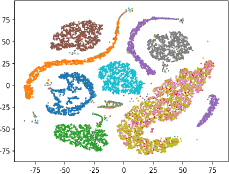
(a) Only cluster-level contrast (NMI=0.821)

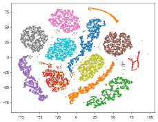
(b) The contrast facet (NMI=0.861)

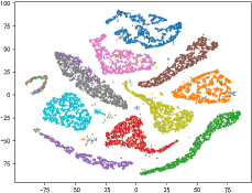
(c) The contrast & feature facets (NMI=0.872)

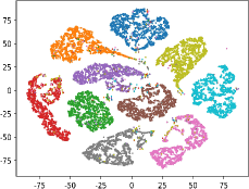
(d) ALL (NMI=0.889)

Figure 1: The qualitative analysis of multifacet complementarity study on Noisy MNIST.

III-A4 Complementarity Investigation

In this section, without loss of generality, we specifically design the investigation experiments for the multifacet complementarity study in the complete MVC setting (i.e., each data point has complete views) and analyze the impact of each facet on the MVC performance quantitatively and qualitatively. Concretely, we take the loss combination of $L_{clu}+L_{rec}$ as Baseline which can be seen as implicitly using view-labels and has been employed in the SOTA method [19].

$$L_{base}=L_{clu}+\mu L_{rec}$$

For the quantitative analysis, we take Caltech101-20 as an example, and adopt three widely-used clustering metrics including Accuracy (ACC), Normalized Mutual Information (NMI), and Adjusted Rand Index (ARI). Let $L_{ins}=L_{mse}$, we run the models 5 times and take their average as the final results. Table 1 reports the results.

As shown in Table 1, compared with Baseline, it can be seen that whether the contrast facet $L_{ins}$ or the feature facet $L_{var}$ is additionally introduced, the corresponding performance can be improved to varying degrees in terms of ACC. However, these gains are rather limited, even both two are introduced jointly. But when we explicitly embed the view-label information, i.e., adding $L_{cla}$ to Baseline, the MVC performance improves remarkably, e.g., ACC($+12.22\%$), NMI($+4.25\%$), and ARI($+22.74\%$). Furthermore, we also conduct an independent experiment with $L_{clu}+L_{cla}$, which remarkably surpasses Baseline as well with ($70.80\%$ vs $55.12\%$) in ACC, ($70.61\%$ vs $66.36\%$) in NMI, and ($80.09\%$ vs $54.09\%$) in ARI. All of these fully demonstrate the importance of view-labels, while indicate that explicitly using them has more advantages than using them implicitly like Baseline, which convincingly answers ’YES’ to the two questions asked in Section 3.1.

In addition, after introducing $L_{cla}$, the MVC performance can be further improved significantly regardless of adding $L_{ins}$ or $L_{var}$. In particular, the performance achieves the optimum, when all of them jointly contribute to the total objective function. This further evidences the importance of view-labels, while showing that all the facets are beneficial to the complementarity learning. Besides, an interesting phenomenon is that when $L_{ins}$ and $L_{var}$ are added alone or at the same time, the performance gains are not significant. However, once $L_{cla}$ is introduced, the performance can be generally significantly improved, which seems to indicate that some intriguing reactions are produced when $L_{cla}$ works together with $L_{ins}$, $L_{var}$ or both, which is worth further investigation in the future.

For the qualitative analysis, we take Noisy MNIST as an example, and show its t-sne visualizations using the loss combinations of different complementarity facets. Fig. 1(a-d) respectively show that the objective uses the cluster-level loss $L_{clu}$, the contrast facet losses (i.e.,$L_{clu}$ and $L_{ins}$), the contrast and feature facet losses (i.e., $L_{clu}$, $L_{ins}$, $L_{rec}$, and $L_{var}$) and all the three facet losses. We can find that with the addition of each loss term by term, the learned representations become more compact in regular shapes, while the clusters are increasingly discriminative with less overlaps. Furthermore, this visual demonstrations are also in line with the increasing performance of NMI. This once again evidences the effectiveness of these three facets.

III-B Multifacet Complementarity Learning Framework

Based on the investigations above, we put forward a multifacet complementarity learning framework (MCMVC), as follows

$$L=L_{\text{The contrast facet}}+L_{\text{The feature facet}}+L_{\text{The view-label facet}}$$

While maintaining the view consistency, MCMVC realizes the complementarity learning of views from the feature facet, view-label facet and contrast facet, especially explicitly embedding view-label information. Fig. 2 shows the overview of the proposed MCMVC. Note that this framework is very flexible and can be implemented by any existing off-the-shelf methods.

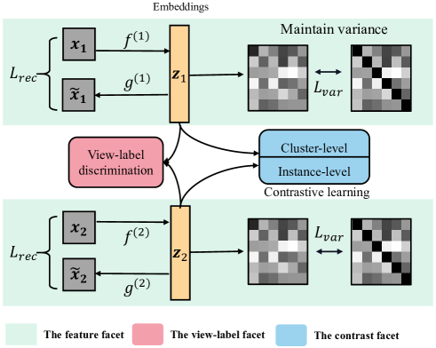
Figure 2: Overview of the MCMVC framework.

III-B1 MCMVC for Bi-view Datasets

The method in [19], i.e., COMPLETER, is specifically designed for bi-view datasets, and obtains the current SOTA performance. Without any change to the backbone network architecture in [19], it can be expanded to our MCMVC by just introducing several additional losses (i.e., $L_{ins},L_{var},L_{cla}$). Compared with [19], though several additional losses are introduced, the scale of network parameters in MCMVC has little change, except that the implementation of the view-label facet loss ($L_{cla}$) introduces an additional linear predictor based on the embedding representation $\bm{z}$, in which the introduced training parameters can be negligible. Concretely, we have the following loss function:

$$L=\underbrace{L_{clu}+\lambda_{1}L_{ins}}_{\text{The contrast facet}}+\underbrace{\lambda_{2}L_{rec}+\lambda_{3}L_{var}}_{\text{The feature facet}}+\underbrace{\lambda_{4}L_{cla}}_{\text{The view-label facet}}$$ (7)

Moreover, using different instance-level contrastive losses, we develop two versions of MCMVC for bi-view datasets, i.e., MCMVC-M using the MSE loss and MCMVC-I using the InfoNCE loss. In addition, we also conduct the incomplete MVC experiments following [19], where a dual prediction loss is additionally introduced as well. It is worth noting that different from [19] which needs a pre-training process to stabilize the training of this loss, our model does not need such a process at all yet it is still stable, as shown in subsection 4.3.3.

III-B2 MCMVC for Datasets with More Views ($\geq 2$)

As mentioned above, the method COMPLETER in [19] is specifically designed for bi-view datasets, and when facing more views ($>2$), the authors do not provide corresponding strategies. Admittedly, it is possible to adapt COMPLETER to the situation of more than two views, but this is beyond the scope of this paper. Thanks to the flexibility of our proposed framework, we here implement it for the situation of more than two views directly on the basis of MFLVC [20] which is the current SOTA method for the datasets with more than two views. For clarity, we call such extended method MCMVC+, which actually can handle the datasets with any number of views. Different from MCMVC-M(I), the key of MCMVC+ is to adapt the contrast facet loss and view-label facet loss to three or more views, which details in the following parts.

The Accumulated Multi-view Contrast Loss. Following [20], the accumulated multi-view contrast loss is introduced at the contrast facet. Specifically, for the instance-level contrast, a feature MLP is stacked on the embedding representation $\{\bm{z}^{v}\}^{V}_{v=1}$ to obtain the instance-level contrast features $\{\bm{H}^{v}\}^{V}_{v=1}$, where $\bm{h}^{v}_{t}\in\mathbb{R}^{H}$ and the feature MLP is one-layer linear MLP denoted by $F(\{\bm{z}^{v}\}^{V}_{v=1};\bm{W}_{H})$. Similar to [20], we adopt NT-Xent loss [22], a variant of InfoNCE loss, to realize the instance-level contrast:

$$l_{ic}^{(ij)}=-\frac{1}{m}\sum^{m}_{t=1}\log\frac{e^{(\text{sim}(\bm{h}_{t}^{i},\bm{h}_{t}^{j})/\tau_{1})}}{\sum_{s=1}^{m}\sum_{v=i,j}e^{(\text{sim}(\bm{h}_{t}^{i},\bm{h}_{s}^{v})/\tau_{1})}-e^{1/\tau_{1}}}$$

Then the accumulated multi-view instance-level contrastive loss can be formulated as:

$$L_{\bm{H}}=\frac{1}{2}\sum_{v=1}^{V}\sum_{i\neq j}l_{fc}^{(ij)}.$$ (8)

For the cluster-level contrast, a cluster MLP, i.e., $F(\{\bm{z}^{v}\}^{V}_{v=1};\bm{W}_{Q})$, is stacked on the embedding representation $\{\bm{z}^{v}\}^{V}_{v=1}$, whose last layer is set to the Softmax operation to output the probability, e.g., $q_{ij}^{v}$ denotes the probability that the $i$-th sample belongs to the $j$-th cluster in the $v$-th view. Thus we can obtain the cluster assignments of samples for all views $\{\bm{Q}^{v}\in\mathbb{R}^{m\times K}\}_{v=1}^{V}$. Similar to the instance-level contrast, the cluster-level contrast can be formulated as

$$l_{cc}^{(ij)}=-\frac{1}{K}\sum^{K}_{t=1}\log\frac{e^{(\text{sim}(\bm{Q}_{\cdot t}^{i},\bm{Q}_{\cdot t}^{j})/\tau_{2})}}{\sum_{s=1}^{K}\sum_{v=i,j}e^{(\text{sim}(\bm{Q}_{\cdot t}^{i},\bm{Q}_{\cdot s}^{v})/\tau_{2})}-e^{1/\tau_{2}}}.$$

Thus we have the following accumulated multi-view cluster-level contrastive loss

$$L_{\bm{Q}}=\frac{1}{2}\sum_{v=1}^{V}\sum_{i\neq j}l_{cc}^{(ij)}+\sum_{v=1}^{V}\sum_{t=1}^{K}u_{t}^{v}\log u_{t}^{v},$$ (9)

where $u_{t}^{v}=\frac{1}{m}\sum_{s=1}^{m}u_{st}^{v}$. The first part of Eq.(9) aims to learn the clustering consistency for all views, while its second part is a regularization term [40] used to avoid all samples being assigned into a single cluster. For more details, we refer the reader to [20].

View-label Prediction for More Views. As for the view-label facet, when facing three or more views, we just need to replace the binary cross entropy loss with its multi-class version as follows:

$$L_{mcla}=-\sum_{v=1}^{V}\sum_{t=1}^{m}\left(y_{t}\log(h(\bm{z}_{t}^{v}))\right),$$ (10)

where $y_{t}$ indicates which view the data $\bm{z}_{t}^{v}$ comes from.

With the feature facet loss, our MCMVC+ can be formulated as

$$L=\underbrace{L_{rec}+\mu_{1}L_{var}}_{\text{The feature facet}}+\underbrace{L_{\bm{Q}}+L_{\bm{H}}}_{\text{The contrast facet}}+\underbrace{\mu_{2}L_{mcla}}_{\text{The view-label facet}}.$$ (11)

MCMVC+ adopts the backbone network architecture provided by [20]. As this backbone network is trained in stages, we first pre-train the backbone network using the feature facet loss, then the contrast facet and view-label facet losses are jointly used to retrain the network. Note that such a training process reduces our need for the large number of weight parameters used to balance the different losses. In fact, we only introduce two weight parameters, i.e., $\mu_{1}$ and $\mu_{2}$ respectively for $L_{var}$ and $L_{mcla}$.

III-B3 MCMVC++

Furthermore, inspired by [20], we also introduce an additional cluster-assignment enhancement module on the basis of MCMVC+ and finally develop the MCMVC++ learning framework. The cluster-assignment enhancement module leverages the cluster information from the instance-level contrast features to further enhance the cluster assignments obtained by the cluster MLP, which details in the following part.

Cluster-assignment Enhancement (CE). Concretely, the $K$-means technique is applied to the instance-level contrast features $\{\bm{H}^{v}\}^{V}_{v=1}$ to obtain the cluster information of each view. For the $v$-th view, letting $\{c_{k}^{v}\}_{k=1}^{K}\in\mathbb{R}^{H}$ denote the $K$ cluster centroids, we have

$$\min_{\bm{c}_{1}^{v},\bm{c}_{2}^{v},...,\bm{c}_{K}^{v}}\sum_{i=1}^{m}\sum_{j=1}^{K}\|\bm{h}_{i}^{v}-\bm{c}_{j}^{v}\|_{2}^{2}.$$ (12)

The cluster assignments of all samples $\bm{p}^{v}\in\mathbb{R}^{m}$ can be obtained by

$$p_{i}^{v}=\arg\min_{j}|\bm{h}_{i}^{v}-\bm{c}_{j}^{v}\|_{2}^{2}.$$ (13)

Let $\bm{l}^{v}\in\mathbb{R}^{m}$ represent the cluster assignment obtained by the cluster MLP, in which $l_{i}^{v}=\arg\max_{j}q_{ij}^{v}$. Note that the clusters denoted by $\bm{p}^{v}$ and $\bm{l}^{v}$ are not corresponding to each other. To achieve the consistent correspondence between them, we can adopt the following maximum matching formula

$$\min_{\bm{A}^{v}}\bm{U}^{v}\bm{A}^{v}$$ (14)

$$s.t.\sum_{i=1}u_{ij}^{v}=1,\ \ \sum_{j=1}^{v}=1,$$

$$a_{ij}^{v}\in\{0,1\},i,j=1,2,...,K,$$

where $\bm{A}^{v}\in\{0,1\}^{K\times K}$ denotes the boolean matrix and $\bm{U}^{v}\in\mathbb{R}^{K\times K}$ represents the cost matrix. $\bm{U}^{v}=\max_{i,j}\widetilde{u}_{ij}^{v}-\bm{\widetilde{U}}^{v}$ and $\widetilde{u}_{ij}^{v}=\sum_{t=1}^{m}\mathbbm{1}[l_{t}^{v}=i]\mathbbm{1}[p_{t}^{v}=j]$, where $\mathbbm{1}$ is the indicator function. The solution of Eq.(14) can be obtained by the Hungarian algorithm [47]. Let $\widehat{\bm{p}}_{i}^{v}\in\{0,1\}^{K}$ denote the modified cluster assignment for the $i$-th sample, which can be used to further enhance the cluster assignments obtained by the cluster MLP by the following loss function

$$L_{\bm{P}}=-\sum_{v=1}^{V}\widehat{\bm{P}}^{v}\log\bm{Q}^{v},$$ (15)

where $\widehat{\bm{P}}^{v}=[\widehat{\bm{p}}_{1}^{v},\widehat{\bm{p}}_{2}^{v},...,\widehat{\bm{p}}_{m}^{v}]\in\mathbb{R}^{m\times K}$. Finally, the cluster assignment of the $i$-th sample is:

$$y_{i}=\arg\max_{j}\left(\frac{1}{V}\sum_{v=1}^{V}q_{ij}^{v}\right).$$ (16)

Overall above, the full optimization process of MCMVC++ is summarized in Algorithm 1.

Remark. Compared with MFLVC [20], though the variance and view-label prediction losses are additionally introduced, the scale of network parameters in MCMVC++ has little change, except that the implementation of the view-label facet loss ($L_{mcla}$) introduces an additional linear predictor based on the embedding representation $\bm{z}$, in which the introduced training parameters can be negligible.

Algorithm 1 The optimization of MCMVC++

1:Multi-view dataset $\{\bm{x}^{v}\}_{v=1}^{V}$; Number of clusters $K$; Temperature parameters $\tau_{1}$ and $\tau_{2}$.

2:Inintialize $\{\theta^{v},\phi^{v}\}_{v=1}^{V}$ by minimizing Eq.(1) and Eq.(2).

3:Optimize $\bm{W}_{H}$, $\bm{W}_{Q}$, $\{\theta^{v}\}_{v=1}^{V}$ by minimizing Eq.(8), Eq.(9) and Eq.(10).

4:Compute cluster assignments by Eq.(12) and Eq.(13).

5:Match multi-view cluster assignments by solving Eq.(14).

6:Fine-tune $\bm{W}_{Q}$, $\{\theta^{v}\}_{v=1}^{V}$ by minimizing Eq.(15).

7:Calculate the final cluster assignment by Eq.(16).

8:The label predictor $\{\{\theta^{v}\}_{v=1}^{V},\bm{W}_{Q}\}$; The high-level feature extractor $\{\{\theta^{v}\}_{v=1}^{V},\bm{W}_{H}\}$.

IV Experiments

IV-A Datasets

For the bi-view experiments, we follow [19] and use the following widely-used dataset:

• Caltech101-20 [48]: has 2386 images from 20 subjects, and the views of HOG and GIST features are used.

• LandUse-21 [49]: owns 2100 satellite images from 21 categories, and the views of PHOG and LBP features are used.

• Scene-15 [50]: consists of 4485 images from 15 categories, and the PHOG and GIST features are used as two views.

• Noisy MNIST [51]: is a multi-view version of MNIST, where the original MNIST images are used as view 1, while the randomly selected within-class images with Gaussian noise are used as view 2. Like [19], we here use a 20k subset of Noise MNIST including 10k validation images and 10k testing images.

For the experiments with more views ($\geq 2$), we follow [20] and use the following widely-used dataset:

• MNIST-USPS [52]: contains 5000 samples from 10 categories, and two different styles of digital images are provided.

• BDGP [53]: contains 2500 samples of drosophila embryos, and two views of visual and textual representations are provided.

• Columbia Consumer Video (CCV) [54]: contains 6773 samples belonging to 20 categories, and three views of hand-crafted Bag-of-Words representations are provided, including STIP, SIFT, and MFCC.

• Fashion [55] contains 10 kinds of fashionable products (such as T-shirt, dress, etc.). Following [56], we treat different three styles as three views of one product.

• Caltech [57]: owns 1400 samples from 7 categories with five view features (i.e., WM, CENTRIST, LBP, GIST, HOG). Based on it, we build four datasets for the evaluations in terms of the number of views like [56]. Concretely, Caltech-2V contains WM and CENTRIST; Caltech-3V contains WM, CENTRIST and LBP; Caltech-4V contains WM, CENTRIST, LBP and GIST; Caltech-5V contains WM, CENTRIST, LBP, GIST and HOG.

IV-B Experimental Settings

To comprehensively evaluate the proposed multifacet complementarity learning framework, we respectively conduct the experiments on benchmark datasets with bi-view and more than two views. Four widely-used metrics, i.e., clustering accuracy (ACC), normalized mutual information (NMI), Adjusted Rand Index (ARI), and purity (PUR), are adopted to evaluate the effectiveness of clustering. We implement our methods (including MCMVC-M(I) and MCMVC++) in PyTorch 1.6.0 and carry all experiments on a standard Ubuntu-16.04 OS with an NVIDIA 2080Ti GPU. Next, we detail the experimental settings about these two types of experiments.

TABLE II: The clustering performance comparisons on the datasets with bi-view under complete MVC setting. ‘-’ indicates unavailable results due to out of memory. Bold denotes the best results ($\%$), while underline denotes the second-best ($\%$).

Method\Datasets	Caltech101-20			LandUse-21			Scene-15			Noisy MNIST
	ACC	NMI	ARI	ACC	NMI	ARI	ACC	NMI	ARI	ACC	NMI	ARI
AE2Nets [15] (2019)	49.10	65.38	35.66	24.79	30.36	10.35	36.10	40.39	22.08	56.98	46.83	36.98
IMG [58] (2016)	44.51	61.35	35.74	16.40	27.11	5.10	24.20	25.64	9.57	-	-	-
UEAF [59] (2019)	47.40	57.90	38.98	23.00	27.05	8.79	34.37	36.69	18.52	67.33	65.37	55.81
DAIMC [60] (2019)	45.48	61.79	32.40	24.35	29.35	10.26	32.09	33.55	17.42	39.18	35.69	23.65
EERIMVC [61] (2020)	43.28	55.04	30.42	24.92	29.57	12.24	39.60	38.99	22.06	65.47	57.69	49.54
DCCAE [51] (2015)	44.05	59.12	34.56	15.62	24.41	4.42	36.44	39.78	21.47	81.60	84.69	70.87
PVC [62] (2014)	44.91	62.13	35.77	25.22	30.45	11.72	30.83	31.05	14.98	41.94	33.90	22.93
BMVC [63] (2018)	42.55	63.63	32.33	25.34	28.56	11.39	40.50	41.20	24.11	81.27	76.12	71.55
DCCA [64] (2013)	41.89	59.14	33.39	15.51	23.15	4.43	36.18	38.92	20.87	85.53	89.44	81.87
PIC [65] (2019)	62.27	67.93	51.56	24.86	29.74	10.48	38.72	40.46	22.12	-	-	-
EAMC [14] (2020)	45.87	41.03	42.31	17.80	19.02	5364	24.83	31.91	12.73	32.57	28.81	15.35
SiMVC [66] (2021)	40.73	63.00	32.65	25.10	31.76	12.06	28.86	28.06	13.05	35.68	28.74	18.06
CoMVC [66] (2021)	38.67	61.48	31.38	25.58	31.92	13.00	30.64	30.31	13.62	41.87	35.02	24.14
COMPLETER [19] (2021)	70.18	68.06	77.88	25.63	31.73	13.05	41.07	44.68	24.78	89.08	88.86	85.47
MCMVC-M (Ours 1)	73.77	71.89	87.26	27.33	32.98	14.34	42.59	45.76	25.95	92.17	86.79	85.22
MCMVC-I (Ours 2)	73.45	71.44	86.73	27.78	33.74	14.90	42.79	46.59	26.74	94.77	88.54	88.88

TABLE III: The clustering performance comparisons on the datasets with bi-view under incomplete MVC setting. ‘-’ indicates unavailable results due to out of memory. Bold denotes the best results ($\%$), while underline denotes the second-best ($\%$).

Method\Datasets	Caltech101-20			LandUse-21			Scene-15			Noisy MNIST
	ACC	NMI	ARI	ACC	NMI	ARI	ACC	NMI	ARI	ACC	NMI	ARI
AE2Nets [15] (2019)	33.61	49.20	24.99	19.22	23.03	5.75	27.88	31.35	13.93	38.67	33.79	19.99
IMG [58] (2016)	42.29	58.26	33.69	15.52	22.54	3.73	23.96	25.70	9.21	-	-	-
UEAF [59] (2019)	47.35	56.71	37.08	16.38	18.42	3.80	28.20	27.01	8.70	34.56	33.13	24.04
DAIMC [60] (2019)	44.63	59.53	32.70	19.30	19.45	5.80	23.60	21.88	9.44	34.44	27.15	16.42
EERIMVC [61] (2020)	40.66	51.38	27.91	22.14	25.18	9.10	33.10	32.11	15.91	54.97	44.91	35.94
DCCAE [51] (2015)	40.01	52.88	30.00	14.94	20.94	3.67	31.75	34.42	15.80	61.79	59.49	33.49
PVC [62] (2014)	41.42	56.53	31.00	21.33	23.14	8.10	25.61	25.31	11.25	35.97	27.74	16.99
BMVC [63] (2018)	32.13	40.58	12.20	18.76	18.73	3.70	30.91	30.23	10.93	24.36	15.11	6.50
DCCA [64] (2013)	38.59	52.51	29.81	14.08	20.02	3.38	31.83	33.19	14.93	61.82	60.55	37.71
PIC [65] (2019)	57.53	64.32	45.22	23.60	26.52	9.45	38.70	37.98	21.16	-	-	-
COMPLETER [19] (2021)	68.44	67.39	75.44	22.16	27.00	10.39	39.50	42.35	23.51	80.01	75.23	70.66
MCMVC-M (Ours 1)	74.84	70.32	88.75	22.65	28.24	11.22	40.07	42.67	24.15	85.88	77.19	74.51
MCMVC-I (Ours 2)	74.14	70.54	87.48	22.90	27.87	11.89	39.94	42.78	24.14	86.35	76.39	73.39

IV-B1 Bi-view Experiment Settings

Following [19], we conduct the bi-view experiments on Caltech101-20, LandUse-21, Scene-15, and Noisy MNIST under both complete and incomplete MVC settings. For the incomplete case, we define the miss rate as $\eta=(n-m)/n$, where $m$ and $n$ denote the number of complete samples and the whole dataset, respectively. For each dataset, we run the models 5 times and take their average as the final results. Meanwhile, ACC, NMI and ARI clustering metrics are used.

Training details. The backbone network of our methods (including MCMVC-M and MCMVC-I) adopts the network architectures from [19], and the dimensionality of the encoders is set to $E-1024-1024-1024-D$, where $E$ is the dimension of raw data and $D$ is the dimension of latent space. The Adam optimizer with default parameters is employed to train our model. The batch size is set to $256$, while the initial learning rate is set to $1e-4$ for Caltech101-20 and $1e-3$ for other three datasets.

For MCMVC-M, in the complete MVC setting, the parameters $\lambda_{2}$, $\lambda_{4}$ are respectively set to 0.1 and 0.2 for all datasets. For Caltech101-20, we set $\lambda_{1}=0.2$ and $\lambda_{3}=0.2$ and train for 500 epochs. For LandUse21, we respectively fix $\lambda_{1}$ and $\lambda_{3}$ to 0.5 and 0.2, and set the training epoch to 1000. For Scene-15, we let $\lambda_{1}=0.1$, $\lambda_{3}=0.3$ and the training epoch be 400. For Noisy MNIST, $\lambda_{1}$ is set to 0.1, $\lambda_{3}$ is set to 0.3 and the training epoch is set to 650. In the incomplete MVC setting, we follow [19] and introduce a dual prediction loss to address the missing view problem, defined as follows

$$L_{pre}=\|G^{(1)}(\bm{z}^{1})-\bm{z}^{2}\|_{2}^{2}+\|G^{(2)}(\bm{z}^{2})-\bm{z}^{1}\|_{2}^{2},$$

where $G^{(j)}(\cdot)$ denotes a parameterized model which maps the embedding representation $\bm{z}^{j}$ of view $j$ to that $\bm{z}^{i}$ of view $i$. For more details, please refer to [19]. We set the weight parameter of $L_{pre}$ to 0.2 recommended by [19] and maintain the parameters used in the complete setting with just slightly modifying $\lambda_{1}$, $\lambda_{3}$ and the training epoch. For Caltech101-20, we maintain the same setting as in complete setting except for modifying the training epoch to 1000. For LandUse21, we set $\lambda_{1}=1.1$, $\lambda_{3}=1.1$ and the training epoch to 400. For Scene-15, we set $\lambda_{1}$ to 0.2, $\lambda_{3}$ to 0.1 and the training epoch to 500. For Noisy MNIST, $\lambda_{1}$ and $\lambda_{3}$ are respectively fixed to 0.3 and 0.4 and the training epoch is 300.

For MCMVC-I, in the complete MVC setting, similar to the complete setting in MCMVC-M, we still maintain most of the settings except that we fix $\lambda_{1}=0.1$. Still $\lambda_{3}$ and the training epoch varies with different datasets. For Caltech101-20, we use $\lambda_{3}=0.2$ and set the training epoch to 500. For LandUse21, we fix $\lambda_{3}$ to 1.0 while setting the training epoch to 700. For Scene-15, we use $\lambda_{3}=0.7$, while the model is trained for 300 epochs. For Noisy MNIST, $\lambda_{3}$ is also set to 1.0 and the training epoch is set to 500. As for the incomplete MVC setting, similar to the incomplete setting in MCMVC-M, we just slightly modify $\lambda_{3}$ and the training epoch. For Caltech101-20, we use $\lambda_{3}=0.3$ and set the training epoch to 1000. For LandUse21, we set $\lambda_{3}=0.7$ and the training epoch to 700. For Scene-15, we set $\lambda_{3}=0.5$ and the training epoch to 500. For Noisy MNIST, $\lambda_{3}$ is fixed to 1.0, and the training epoch is 200.

IV-B2 Experiment Settings with More Views ($\geq 2$)

Following [20], we conduct the experiments with more views ($\geq 2$) on MNIST-USPS, BDGP, CCV, Fashion, and Caltech-2V, 3V, 4V, 5V in the complete MVC settings. For each dataset, we run the models 10 times and take their average as the final results. Meanwhile, ACC, NMI and PUR clustering metrics are used.

Training details. The backbone network of our MCMVC++ adopts the network architectures from [20], and the dimensionality of the encoders is set to $E-2000-2000-500-500-D$, where $E$ is the dimension of raw data and $D$ is the dimension of latent space. The Adam optimizer with default parameters is employed to train our model. The batch size is set to $256$, while the initial learning rate is set to $3e-4$ for MNIST-USPS, BDGP, Caltech-2V, 3V, 4V, 5V, and $5e-4$ for CCV, $1e-4$ for Fashion. The temperature parameter $\tau_{1}$ is set to $1.0$ for MNIST-USPS and BDGP, The epoches of contrast training process are set to 70, 80, and 70 respectively for Caltech-2V, 3V, and 4V, while other related parameters are set to the default parameters recommended by [20]. As for the weight parameters $\mu_{1}$ and $\mu_{2}$ in Eq.(11), we set $\mu_{1}=0.1,\mu_{2}=0.1$ for MNIST-USPS; $\mu_{1}=0.0001,\mu_{2}=0.03$ for BDGP; $\mu_{1}=0.001,\mu_{2}=0.2$ for CCV; $\mu_{1}=0.1,\mu_{2}=0.4$ for Fashion; $\mu_{1}=0.2,\mu_{2}=0.02$ for Caltech-2V; $\mu_{1}=0.01,\mu_{2}=0.2$ for Caltech-3V; $\mu_{1}=0.1,\mu_{2}=0.4$ for Caltech-4V; $\mu_{1}=0.02,\mu_{2}=0.03$ for Caltech-5V.

IV-C Results on Datasets with Bi-view

IV-C1 Comparisons with State of the Arts

On the bi-view datasets, we conduct the comparisons under the complete and incomplete MVC settings.

In the complete setting, we compare MCMVC-M(I) with 14 leading MVC methods including Deep Canonically Correlated Analysis (DCCA) [64], Deep Canonically Correlated Autoencoders (DCCAE) [51], Binary Multi-view Clustering (BMVC) [63], Autoencoder in Autoencoder Networks (AE²-Nets) [15], Partial Multi-View Clustering (PVC) [62], Efficient and Effective Regularized Incomplete Multi-view Clustering (EERIMVC) [61], Doubly Aligned Incomplete Multi-view Clustering (DAIMC) [60], Incomplete Multi-Modal Visual Data Grouping (IMG) [58], Unified Embedding Alignment Framework (UEAF) [59], Perturbation oriented Incomplete Multi-view Clustering (PIC) [65], Incomplete Multi-view clustering via Contrastive Prediction (COMPLETER) [19], End-to-End Adversarial-Attention Network for Multi-Modal Clustering (EAMC) [14], Simple Multi-View Clustering (SiMVC) [66] and Contrastive Multi-View Clustering (CoMVC) [66]. For fair comparisons, we adopt the same experimental setting as [19] so that we here directly compare with their published results from [19] for the first 10 methods. As for EAMC, SiMVC and CoMVC, we use the recommended network structures and parameters to implement by ourselves. Table 2 reports the results.

As shown in Table 2, MCMVC-M(I) significantly outperforms these leading baselines by a large margin on all four datasets through the multifacet complementarity learning. Compared with the SOTA baseline (i.e., COMPLETER), our MCMVC-M achieves the remarkable improvements by average margins respectively over 2.40% in terms of ACC, 1.00% in terms of NMI, and 2.90% in terms of ARI, while for our MCMVC-I, such margins are even raised to 3.20% in terms of ACC, 1.70% for NMI, and 4.00% for ARI. In particular, MCMVC-I gains a nontrivial $8.85\%$ improvement on Caltech101-20 in terms of ARI.

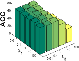
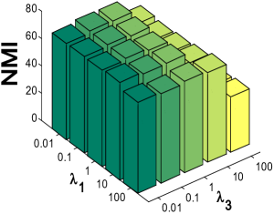
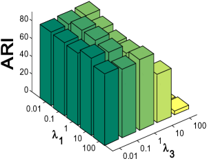
Figure 3: Parameter sensitivity analysis on Caltech101-20.

In the incomplete setting, we also adopt the same experimental setting as [19] for fair comparisons, where the missing rate $\eta$ is set to $0.5$. We compare MCMVC-M(I) with AE²Nets, IMG, UEAF, DAIMC, EERIMVC, DCCAE, PVC, BMVC, DCCA, PIC, COMPLETER, and we here directly compare with their published results from [19]. Table 3 reports the results.

As shown in Table 3, MCMVC-M(I) also achieves significant improvements on most datasets. For example, MCMVC-M wins the best baseline by average margins respectively $3.30\%$ in terms of ACC, $1.60\%$ in terms of NMI, and $4.60\%$ in terms of ARI, while MCMVC-I also has a similar significant performance gains. In particular, both MCMVC-M and MCMVC-I achieve the performance gains of more than $10\%$ on Caltech101-20 in terms of ARI.

Remark. It worth noting that the ACC and ARI performances of our MCMVC in the incomplete setting on Caltech101-20 are surprisingly slightly better than the complete counterpart, which may be a little bit confusing. We conjecture that through considering the mlutifacet complementarity learning, our model captures the richer complementarity information while maintaining the consistency among views. When this information is used to recover the missing views, in some cases, the benefits of the new recovered views may be more than the raw views directly collected, which further demonstrates the advantages of our MCMVC.

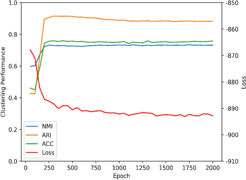
Figure 4: Clustering performance of MCMVC with increasing epoch on Caltech101-20. The x-axis denotes the training epoch, the left and right y-axis denote the clustering performance and corresponding loss value, respectively.

TABLE IV: The clustering performance comparisons on the datasets with more views ($\geq 2$) under complete MVC setting. Bold denotes the best results, while underline denotes the second-best.

Method\Dataset	MNIST-USPS			BDGP			CCV			Fashion
	ACC	NMI	PUR	ACC	NMI	PUR	ACC	NMI	PUR	ACC	NMI	PUR
RMSL [67] (2019)	0.424	0.318	0.428	0.849	0.630	0.849	0.215	0.157	0.243	0.408	0.405	0.421
MVC-LFA [68] (2019)	0.768	0.675	0.768	0.564	0.395	0.612	0.232	0.195	0.261	0.791	0.759	0.794
COMIC [52] (2019)	0.482	0.709	0.531	0.578	0.642	0.639	0.157	0.081	0.157	0.578	0.642	0.608
CDIMC-net [69] (2020)	0.620	0.676	0.647	0.884	0.799	0.885	0.201	0.171	0.218	0.776	0.809	0.789
EAMC [14] (2020)	0.735	0.837	0.778	0.681	0.480	0.697	0.263	0.267	0.274	0.614	0.608	0.638
IMVTSC-MVI [70] (2021)	0.669	0.592	0.717	0.981	0.950	0.982	0.117	0.060	0.158	0.632	0.648	0.635
SiMVC [66] (2021)	0.981	0.962	0.981	0.704	0.545	0.723	0.151	0.125	0.216	0.825	0.839	0.825
CoMVC [66] (2021)	0.987	0.976	0.989	0.802	0.670	0.803	0.296	0.286	0.297	0.857	0.864	0.863
MFLVC [20] (2022)	0.995	0.985	0.995	0.989	0.966	0.989	0.312	0.316	0.339	0.992	0.980	0.992
MFLVC+ (Ours)	0.996	0.987	0.996	0.990	0.967	0.990	0.323	0.319	0.354	0.994	0.984	0.994
MCMVC++ (Ours)	0.996	0.988	0.996	0.990	0.965	0.990	0.334	0.321	0.360	0.994	0.984	0.994

TABLE V: The clustering performance comparisons on the datasets with more views ($\geq 2$) under complete MVC setting. Bold denotes the best results, while underline denotes the second-best.

Method\Datasets	Caltech-2V			Caltech-3V			Caltech-4V			Caltech-5V
	ACC	NMI	PUR	ACC	NMI	PUR	ACC	NMI	PUR	ACC	NMI	PUR
RMSL[67] (2019)	0.525	0.474	0.540	0.554	0.480	0.554	0.596	0.551	0.608	0.354	0.340	0.391
MVC-LFA[68] (2019)	0.462	0.348	0.496	0.551	0.423	0.578	0.609	0.522	0.636	0.741	0.601	0.747
COMIC[52] (2019)	0.422	0.446	0.535	0.447	0.491	0.575	0.637	0.609	0.764	0.532	0.549	0.604
CDIMC-net[69] (2020)	0.515	0.480	0.564	0.528	0.483	0.565	0.560	0.564	0.617	0.727	0.692	0.742
EAMC[14] (2020)	0.419	0.256	0.427	0.389	0.214	0.398	0.356	0.205	0.370	0.318	0.173	0.342
IMVTSC-MVI[70] (2021)	0.490	0.398	0.540	0.558	0.445	0.576	0.687	0.610	0.719	0.760	0.691	0.785
SiMVC[66] (2021)	0.508	0.471	0.557	0.569	0.495	0.591	0.619	0.536	0.630	0.719	0.677	0.729
CoMVC[66] (2021)	0.466	0.426	0.527	0.541	0.504	0.584	0.568	0.569	0.646	0.700	0.687	0.746
MFLVC[20] (2022)	0.606	0.528	0.616	0.631	0.566	0.639	0.733	0.652	0.734	0.804	0.703	0.804
MFLVC+ (Ours)	0.626	0.538	0.631	0.658	0.582	0.666	0.750	0.679	0.753	0.839	0.745	0.839
MCMVC++ (Ours)	0.639	0.554	0.648	0.686	0.604	0.697	0.768	0.675	0.771	0.844	0.754	0.844

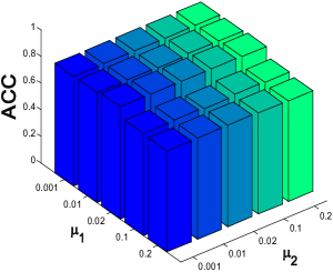
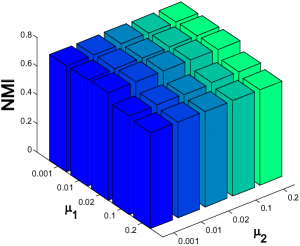
Figure 5: Parameter sensitivity analysis on Caltech-5V.

IV-C2 Parameter Sensitivity Analysis

In this part, we evaluate MCMVC’s sensitivity (using MCMVC-M) to the hyper-parameters on Caltech101-20. On the bi-view situation, we find the weight parameters $\lambda_{2}$ and $\lambda_{4}$ respectively for $L_{rec}$ and $L_{cla}$ are very insensitive. Therefore, we here just conduct sensitivity experiments on the parameters $\lambda_{1}$ and $\lambda_{3}$. We change their value in the range of {0.01, 0.1, 1, 10, 100}. As shown in Fig. 3, our model is also relatively insensitive to the choice of $\lambda_{1}$, $\lambda_{3}$. When $\lambda_{3}$ is larger than 10, MCMVC’s performance decreases rapidly, while the results are still encouraging when $\lambda_{3}$ is smaller than 1. Still, careful selection of these hyper-parameters would result in better performance.

TABLE VI: The clustering performance comparisons on the Cluster-assignment Enhancement (CE). Bold denotes the best results.

Method\Dataset	MNIST-USPS			BDGP			CCV			Fashion
	ACC	NMI	PUR	ACC	NMI	PUR	ACC	NMI	PUR	ACC	NMI	PUR
MCMVC+ (W/O CE)	0.996	0.987	0.996	0.990	0.966	0.990	0.301	0.314	0.349	0.993	0.983	0.993
MCMVC++ (W/ CE)	0.996	0.988	0.996	0.990	0.965	0.990	0.334	0.321	0.360	0.994	0.984	0.994

TABLE VII: The clustering performance comparisons on the Cluster-assignment Enhancement (CE). Bold denotes the best results.

Method\Dataset	Caltech-2V			Caltech-3V			Caltech-4V			Caltech-5V
	ACC	NMI	PUR	ACC	NMI	PUR	ACC	NMI	PUR	ACC	NMI	PUR
MCMVC+ (W/O CE)	0.625	0.541	0.636	0.690	0.606	0.701	0.753	0.661	0.758	0.833	0.736	0.833
MCMVC++ (W/ CE)	0.639	0.554	0.648	0.686	0.604	0.697	0.768	0.675	0.771	0.844	0.754	0.844

IV-C3 Convergence Analysis

In this part, we analyze the convergence of MCMVC (using MCMVC-M) by recording its performance metrics (ACC, NMI, ARI) and its loss with increasing epoches on Caltech101-20. As shown in Fig. 4, the loss decreases remarkably, while the performance increases rapidly for the first 300 epochs. After that, they become relatively stable. In addition, without the pre-training process like [19], our method still performs relatively smoothly throughout the whole training process. We speculate that this may be the result caused by the joint efforts of the losses from all facets.

IV-D Results on Datasets with More Views ($\geq 2$)

IV-D1 Comparisons with State of the Arts

When facing more views $\geq 2$, we develop MCMVC++, and compare it with 9 classical and leading MVC methods including Reciprocal Multi-Layer Subspace Learning (RMSL) [67], Multi-view Clustering via Late Fusion Alignment Maximization (MVC-LFA) [68], Cross-view Matching Clustering (COMIC) [52], Incomplete Multi-view Tensor Spectral Clustering with Missing View Inferring (IMVTSC-MVI) [70], Cognitive Deep Incomplete Multi-view Clustering Network (CDIMC-net) [69], End-to-End Adversarial-Attention Network for Multi-Modal Clustering (EAMC) [14], Simple Multi-View Clustering (SiMVC) [66], Contrastive Multi-View Clustering (CoMVC) [66], and Multi-level Feature Learning for Contrastive Multi-view Clustering (MFLVC) [20].

For fair comparisons, we adopt the same experimental setting as [20] so that we here directly compare with their published results from [20] for the first 9 methods. Moreover, to further verify the importance of view-labels, we also develop an enhanced version MFLVC, i.e., MFLVC+, which additionally introduces the view-label prediction loss $L_{mcla}$. Note that the implementation of $L_{mcla}$ just adds a linear predictor based on the embedding representation $\bm{z}$, in which the introduced training parameters can be negligible.

Table 4 reports the results on MNIST-USPS, BDGP, CCV, and Fashion. As shown in Table 4, both MFLVC+ and MCMVC++ have at least a slight lead over the SOTA baseline MFLVC on all these datasets. Please note that the performances on MNIST-USPS, BDGP, and Fashion are almost saturated (Close to $100\%$), and even a small performance gain is very difficult. This demonstrates the utilities of view-label and variance losses to some extent.

To further verify our methods, we follow [20] and conduct the experiments on Caltech-2V, 3V, 4V, and 5V. Table 5 shows the results, and from which we can find that: (1) the introduction of view-label prediction does endow the original MFLVC more powerful capabilities, where MFLVC+ beats MFLVC in terms of all metrics on all datasets, e.g., by average margins $2.48\%$ in ACC, $2.38\%$ in NMI, and $2.40\%$ in PUR, which once again fully indicates the importance of view-labels. (2) Based on MFLVC+, the further addition of variance loss term, i.e., our MCMVC++, further improves the performance. For example, MCMVC++ wins MFLVC+ by $1.3\%$ on Caltech-2V, $2.6\%$ on Caltech-3V, $1.8\%$ on Caltech-4V, and $0.5\%$ on Caltch-5V in terms of ACC. (3) In particular, compared with the SOTA baseline (i.e., MFLVC), our MCMVC++ achieves remarkable improvements, by average margins respectively over $4.03\%$ in terms of ACC, $3.35\%$ in terms of NMI, and $4.18\%$ in terms of ARI on all Caltech datasets, which also once again evidences the effectiveness of these three facets.

IV-D2 Parameter Sensitivity Analysis

In this part, we evaluate MCMVC++’s sensitivity to the hyper-parameters $\mu_{1}$ and $\mu_{2}$ on Caltech-5V. We change their value in the range of {0.001, 0.01, 0.02, 0.1, 0.2}. As shown in Fig. 5, our model is relatively insensitive to the choice of $\mu_{1}$, $\mu_{2}$. Still, careful selection of these hyper-parameters would result in better performance.

IV-D3 The Impact of Cluster-assignment Enhancement

In this part, we evaluate the impact of cluster-assignment enhancement on the performance. Table 6 and Table 7 report the results. As shown in Table 6 and Table 7, The introduction of cluster-assignment enhancement does further improve the performance of the model. MCMVC++ beats MCMVC+ in all metrics on most datasets, except for Caltech-3V and BDGP, where it is comparable, e.g., $0.686$ vs $0.690$ in terms of ACC, $0.604$ vs $0.606$ in terms of NMI, and $0.697$ vs $0.701$ in terms of PUR on Caltech-3V.

V Conclusion

This paper explores a multifacet complementarity study of MVC from the feature facet, view-label facet, and contrast facet, in which we find that all three facets jointly contribute to the complementarity learning of views, especially the view-label facet which is usually ignored or has never been explicitly concerned by existing works. Based on our such findings, we propose the multifacet complementarity learning framework for multi-view clustering. Specifically, we respectively develop MCMVC-M(I) and MCMVC++ for datasets with bi-view and more than two views. Their excellent performance on all datasets also supports our conclusions in turn. What needs special emphasis is that our novel view-label facet is orthogonal to all the facets in all existing MVC methods, meaning it can also boost their performance.

References

- [1] A. Blum and T. Mitchell, “Combining labeled and unlabeled data with co-training,” in Proceedings of the eleventh annual conference on Computational learning theory, 1998, pp. 92–100.
- [2] X. Cao, C. Zhang, H. Fu, S. Liu, and H. Zhang, “Diversity-induced multi-view subspace clustering,” in Proceedings of the IEEE conference on computer vision and pattern recognition, 2015, pp. 586–594.
- [3] J. Zhao, X. Xie, X. Xu, and S. Sun, “Multi-view learning overview: Recent progress and new challenges,” Information Fusion, vol. 38, pp. 43–54, 2017.
- [4] Y. Li, M. Yang, and Z. Zhang, “A survey of multi-view representation learning,” IEEE transactions on knowledge and data engineering, vol. 31, no. 10, pp. 1863–1883, 2018.
- [5] A. Kumar, P. Rai, and H. Daume, “Co-regularized multi-view spectral clustering,” Advances in neural information processing systems, vol. 24, pp. 1413–1421, 2011.
- [6] J. Liu, C. Wang, J. Gao, and J. Han, “Multi-view clustering via joint nonnegative matrix factorization,” in Proceedings of the 2013 SIAM international conference on data mining. SIAM, 2013, pp. 252–260.
- [7] M. D. Collins, J. Liu, J. Xu, L. Mukherjee, and V. Singh, “Spectral clustering with a convex regularizer on millions of images,” in European Conference on Computer Vision. Springer, 2014, pp. 282–298.
- [8] H. Gao, F. Nie, X. Li, and H. Huang, “Multi-view subspace clustering,” in Proceedings of the IEEE international conference on computer vision, 2015, pp. 4238–4246.
- [9] W. Wang and Z.-H. Zhou, “Analyzing co-training style algorithms,” in European conference on machine learning. Springer, 2007, pp. 454–465.
- [10] X. Wang, X. Guo, Z. Lei, C. Zhang, and S. Z. Li, “Exclusivity-consistency regularized multi-view subspace clustering,” in Proceedings of the IEEE conference on computer vision and pattern recognition, 2017, pp. 923–931.
- [11] S. Luo, C. Zhang, W. Zhang, and X. Cao, “Consistent and specific multi-view subspace clustering,” in Thirty-second AAAI conference on artificial intelligence, 2018.
- [12] Z. Li, C. Tang, J. Chen, C. Wan, W. Yan, and X. Liu, “Diversity and consistency learning guided spectral embedding for multi-view clustering,” Neurocomputing, vol. 370, pp. 128–139, 2019.
- [13] X. Si, Q. Yin, X. Zhao, and L. Yao, “Consistent and diverse multi-view subspace clustering with structure constraint,” Pattern Recognition, vol. 121, p. 108196, 2022.
- [14] R. Zhou and Y.-D. Shen, “End-to-end adversarial-attention network for multi-modal clustering,” in Proceedings of the IEEE/CVF Conference on Computer Vision and Pattern Recognition, 2020, pp. 14 619–14 628.
- [15] C. Zhang, Y. Liu, and H. Fu, “Ae2-nets: Autoencoder in autoencoder networks,” in Proceedings of the IEEE/CVF Conference on Computer Vision and Pattern Recognition, 2019, pp. 2577–2585.
- [16] Z. Huang, J. T. Zhou, X. Peng, C. Zhang, H. Zhu, and J. Lv, “Multi-view spectral clustering network.” in IJCAI, 2019, pp. 2563–2569.
- [17] P. Zhu, B. Hui, C. Zhang, D. Du, L. Wen, and Q. Hu, “Multi-view deep subspace clustering networks,” arXiv preprint arXiv:1908.01978, 2019.
- [18] J. Xu, Y. Ren, G. Li, L. Pan, C. Zhu, and Z. Xu, “Deep embedded multi-view clustering with collaborative training,” Information Sciences, vol. 573, pp. 279–290, 2021.
- [19] Y. Lin, Y. Gou, Z. Liu, B. Li, J. Lv, and X. Peng, “Completer: Incomplete multi-view clustering via contrastive prediction,” in Proceedings of the IEEE/CVF Conference on Computer Vision and Pattern Recognition, 2021, pp. 11 174–11 183.
- [20] J. Xu, H. Tang, Y. Ren, L. Peng, X. Zhu, and L. He, “Multi-level feature learning for contrastive multi-view clustering,” in Proceedings of the IEEE/CVF Conference on Computer Vision and Pattern Recognition, 2022, pp. 16 051–16 060.
- [21] K. He, H. Fan, Y. Wu, S. Xie, and R. Girshick, “Momentum contrast for unsupervised visual representation learning,” in Proceedings of the IEEE/CVF Conference on Computer Vision and Pattern Recognition, 2020, pp. 9729–9738.
- [22] T. Chen, S. Kornblith, M. Norouzi, and G. Hinton, “A simple framework for contrastive learning of visual representations,” in International conference on machine learning. PMLR, 2020, pp. 1597–1607.
- [23] A. Bardes, J. Ponce, and Y. LeCun, “Vicreg: Variance-invariance-covariance regularization for self-supervised learning,” arXiv preprint arXiv:2105.04906, 2021.
- [24] C. Zhang, H. Fu, Q. Hu, X. Cao, Y. Xie, D. Tao, and D. Xu, “Generalized latent multi-view subspace clustering,” IEEE transactions on pattern analysis and machine intelligence, vol. 42, no. 1, pp. 86–99, 2018.
- [25] S. Huang, I. W. Tsang, Z. Xu, J. Lv, and Q. Liu, “Cdd: Multi-view subspace clustering via cross-view diversity detection,” in Proceedings of the 29th ACM International Conference on Multimedia, 2021, pp. 2308–2316.
- [26] Y. Wang, L. Wu, X. Lin, and J. Gao, “Multiview spectral clustering via structured low-rank matrix factorization,” IEEE transactions on neural networks and learning systems, vol. 29, no. 10, pp. 4833–4843, 2018.
- [27] F. Nie, S. Shi, and X. Li, “Auto-weighted multi-view co-clustering via fast matrix factorization,” Pattern Recognition, vol. 102, p. 107207, 2020.
- [28] R. Wang, F. Nie, Z. Wang, H. Hu, and X. Li, “Parameter-free weighted multi-view projected clustering with structured graph learning,” IEEE Transactions on Knowledge and Data Engineering, vol. 32, no. 10, pp. 2014–2025, 2019.
- [29] X. Li, H. Zhang, R. Wang, and F. Nie, “Multiview clustering: A scalable and parameter-free bipartite graph fusion method,” IEEE Transactions on Pattern Analysis and Machine Intelligence, vol. 44, no. 1, pp. 330–344, 2020.
- [30] S. Huang, I. Tsang, Z. Xu, and J. C. Lv, “Measuring diversity in graph learning: a unified framework for structured multi-view clustering,” IEEE Transactions on Knowledge and Data Engineering, 2021.
- [31] D. Wu, F. Nie, X. Dong, R. Wang, and X. Li, “Parameter-free consensus embedding learning for multiview graph-based clustering,” IEEE Transactions on Neural Networks and Learning Systems, 2021.
- [32] S. Huang, I. W. Tsang, Z. Xu, and J. Lv, “Latent representation guided multi-view clustering,” IEEE Transactions on Knowledge and Data Engineering, 2022.
- [33] L. Du, P. Zhou, L. Shi, H. Wang, M. Fan, W. Wang, and Y.-D. Shen, “Robust multiple kernel k-means using l21-norm,” in Twenty-fourth international joint conference on artificial intelligence, 2015.
- [34] X. Liu, X. Zhu, M. Li, L. Wang, C. Tang, J. Yin, D. Shen, H. Wang, and W. Gao, “Late fusion incomplete multi-view clustering,” IEEE transactions on pattern analysis and machine intelligence, vol. 41, no. 10, pp. 2410–2423, 2018.
- [35] X. Liu, “Incomplete multiple kernel alignment maximization for clustering,” IEEE Transactions on Pattern Analysis and Machine Intelligence, 2021.
- [36] Z. Li, Q. Wang, Z. Tao, Q. Gao, Z. Yang et al., “Deep adversarial multi-view clustering network.” in IJCAI, 2019, pp. 2952–2958.
- [37] C. Zhang, Y. Cui, Z. Han, J. T. Zhou, H. Fu, and Q. Hu, “Deep partial multi-view learning,” IEEE transactions on pattern analysis and machine intelligence, 2020.
- [38] Q. Wang, Z. Tao, W. Xia, Q. Gao, X. Cao, and L. Jiao, “Adversarial multiview clustering networks with adaptive fusion,” IEEE Transactions on Neural Networks and Learning Systems, 2022.
- [39] Y. Yang and H. Wang, “Multi-view clustering: A survey,” Big Data Mining and Analytics, vol. 1, no. 2, pp. 83–107, 2018.
- [40] Y. Wang, “Survey on deep multi-modal data analytics: collaboration, rivalry, and fusion,” ACM Transactions on Multimedia Computing, Communications, and Applications (TOMM), vol. 17, no. 1s, pp. 1–25, 2021.
- [41] T. Wang and P. Isola, “Understanding contrastive representation learning through alignment and uniformity on the hypersphere,” in International Conference on Machine Learning. PMLR, 2020, pp. 9929–9939.
- [42] S. Chen and C. Geng, “A comprehensive perspective of contrastive self-supervised learning,” Frontiers of Computer Science, vol. 15, no. 4, pp. 1–3, 2021.
- [43] J.-B. Grill, F. Strub, F. Altché, C. Tallec, P. Richemond, E. Buchatskaya, C. Doersch, B. Avila Pires, Z. Guo, M. Gheshlaghi Azar et al., “Bootstrap your own latent-a new approach to self-supervised learning,” Advances in Neural Information Processing Systems, vol. 33, pp. 21 271–21 284, 2020.
- [44] X. Chen and K. He, “Exploring simple siamese representation learning,” in Proceedings of the IEEE/CVF Conference on Computer Vision and Pattern Recognition, 2021, pp. 15 750–15 758.
- [45] M. Caron, I. Misra, J. Mairal, P. Goyal, P. Bojanowski, and A. Joulin, “Unsupervised learning of visual features by contrasting cluster assignments,” Advances in Neural Information Processing Systems, vol. 33, pp. 9912–9924, 2020.
- [46] X. Liu, F. Zhang, Z. Hou, L. Mian, Z. Wang, J. Zhang, and J. Tang, “Self-supervised learning: Generative or contrastive,” IEEE Transactions on Knowledge and Data Engineering, 2021.
- [47] R. Jonker and T. Volgenant, “Improving the hungarian assignment algorithm,” Operations Research Letters, vol. 5, no. 4, pp. 171–175, 1986.
- [48] Y. Li, F. Nie, H. Huang, and J. Huang, “Large-scale multi-view spectral clustering via bipartite graph,” in Twenty-ninth AAAI conference on artificial intelligence, 2015.
- [49] Y. Yang and S. Newsam, “Bag-of-visual-words and spatial extensions for land-use classification,” in Proceedings of the 18th SIGSPATIAL international conference on advances in geographic information systems, 2010, pp. 270–279.
- [50] L. Fei-Fei and P. Perona, “A bayesian hierarchical model for learning natural scene categories,” in 2005 IEEE Computer Society Conference on Computer Vision and Pattern Recognition (CVPR’05), vol. 2. IEEE, 2005, pp. 524–531.
- [51] W. Wang, R. Arora, K. Livescu, and J. Bilmes, “On deep multi-view representation learning,” in International conference on machine learning. PMLR, 2015, pp. 1083–1092.
- [52] X. Peng, Z. Huang, J. Lv, H. Zhu, and J. T. Zhou, “Comic: Multi-view clustering without parameter selection,” in International conference on machine learning. PMLR, 2019, pp. 5092–5101.
- [53] X. Cai, H. Wang, H. Huang, and C. Ding, “Joint stage recognition and anatomical annotation of drosophila gene expression patterns,” Bioinformatics, vol. 28, no. 12, pp. i16–i24, 2012.
- [54] Y.-G. Jiang, G. Ye, S.-F. Chang, D. Ellis, and A. C. Loui, “Consumer video understanding: A benchmark database and an evaluation of human and machine performance,” in Proceedings of the 1st ACM International Conference on Multimedia Retrieval, 2011, pp. 1–8.
- [55] H. Xiao, K. Rasul, and R. Vollgraf, “Fashion-mnist: a novel image dataset for benchmarking machine learning algorithms,” arXiv preprint arXiv:1708.07747, 2017.
- [56] J. Xu, Y. Ren, H. Tang, X. Pu, X. Zhu, M. Zeng, and L. He, “Multi-vae: Learning disentangled view-common and view-peculiar visual representations for multi-view clustering,” in Proceedings of the IEEE/CVF International Conference on Computer Vision, 2021, pp. 9234–9243.
- [57] L. Fei-Fei, R. Fergus, and P. Perona, “Learning generative visual models from few training examples: An incremental bayesian approach tested on 101 object categories,” in 2004 conference on computer vision and pattern recognition workshop. IEEE, 2004, pp. 178–178.
- [58] H. Zhao, H. Liu, and Y. Fu, “Incomplete multi-modal visual data grouping.” in IJCAI, 2016, pp. 2392–2398.
- [59] J. Wen, Z. Zhang, Y. Xu, B. Zhang, L. Fei, and H. Liu, “Unified embedding alignment with missing views inferring for incomplete multi-view clustering,” in Proceedings of the AAAI Conference on Artificial Intelligence, vol. 33, no. 01, 2019, pp. 5393–5400.
- [60] M. Hu and S. Chen, “Doubly aligned incomplete multi-view clustering,” in IJCAI, 2018, pp. 2262–2268.
- [61] X. Liu, M. Li, C. Tang, J. Xia, J. Xiong, L. Liu, M. Kloft, and E. Zhu, “Efficient and effective regularized incomplete multi-view clustering,” IEEE transactions on pattern analysis and machine intelligence, 2020.
- [62] S.-Y. Li, Y. Jiang, and Z.-H. Zhou, “Partial multi-view clustering,” in Proceedings of the AAAI conference on artificial intelligence, vol. 28, no. 1, 2014.
- [63] Z. Zhang, L. Liu, F. Shen, H. T. Shen, and L. Shao, “Binary multi-view clustering,” IEEE transactions on pattern analysis and machine intelligence, vol. 41, no. 7, pp. 1774–1782, 2018.
- [64] G. Andrew, R. Arora, J. Bilmes, and K. Livescu, “Deep canonical correlation analysis,” in International conference on machine learning. PMLR, 2013, pp. 1247–1255.
- [65] H. Wang, L. Zong, B. Liu, Y. Yang, and W. Zhou, “Spectral perturbation meets incomplete multi-view data,” in IJCAI, 2019, pp. 3677–3683.
- [66] D. J. Trosten, S. Lokse, R. Jenssen, and M. Kampffmeyer, “Reconsidering representation alignment for multi-view clustering,” in Proceedings of the IEEE/CVF Conference on Computer Vision and Pattern Recognition, 2021, pp. 1255–1265.
- [67] R. Li, C. Zhang, H. Fu, X. Peng, T. Zhou, and Q. Hu, “Reciprocal multi-layer subspace learning for multi-view clustering,” in Proceedings of the IEEE/CVF International Conference on Computer Vision, 2019, pp. 8172–8180.
- [68] S. Wang, X. Liu, E. Zhu, C. Tang, J. Liu, J. Hu, J. Xia, and J. Yin, “Multi-view clustering via late fusion alignment maximization.” in IJCAI, 2019, pp. 3778–3784.
- [69] J. Wen, Z. Zhang, Y. Xu, L. Zhang Bob, Fei, and G.-S. Xie, “Cdimc-net: Cognitive deep incomplete multi-view clustering network,” in IJCAI, 2020, pp. 3230–3236.
- [70] J. Wen, Z. Zhang, Z. Zhang, L. Zhu, L. Fei, B. Zhang, and Y. Xu, “Unified tensor framework for incomplete multi-view clustering and missing-view inferring,” in Proceedings of the AAAI conference on artificial intelligence, vol. 35, no. 11, 2021, pp. 10 273–10 281.