Orbital equivalence classes of finite coverings of geodesic flows

Abstract $-$ Let $M$ be a closed $3$-manifold admitting a finite cover of index $n$ along the fibers over the unit tangent bundle of a closed surface. We prove that if $n$ is odd, there is only one Anosov flow on $M$ up to orbital equivalence, and if $n$ is even, there are two orbital equivalence classes of Anosov flows on $M.$

1. Introduction

Let $\Sigma$ be a closed orientable surface of genus $g>1$, equipped with a negatively curved riemannian metric, and let $T^{1}\Sigma$ be the unit tangent bundle. The geodesic flow $\Phi_{0}^{t}$ on $T^{1}\Sigma$ is a typical Anosov flow (see Section 3.1 for a definition of the geodesic flow, and Definition 2.1 for a definition of Anosov flows).

E. Ghys, in [Gh1], proved that, up to finite covers, geodesic flows are essentially the only possible Anosov flows on circle bundles over a closed surface. More precisely, if $\Phi^{t}$ is an Anosov flow on a closed manifold $M$ admitting a circle fibration over the closed surface $\Sigma$, then there is a finite covering $q:M\to T^{1}(\Sigma)$ such that $\Phi^{t}$ is a reparametrization of the lifting in $M$ by $q$ of the geodesic flow on $T^{1}\Sigma$ (see Theorem 3.3).

Observe that the finite covering $q$ is along the fibers (see Section 3.3). It implies that if $M$ is homeomorphic the unit tangent bundle $T^{1}M$ itself, then $q$ is a homeomorphism, and that, in this case, $\Phi^{t}$ is merely orbitally equivalent to the geodesic flow itself (see Definition 2.3).

This is not true in the general case. More precisely: let $M$ be a closed $3$-manifold admitting a circle fibration over $\Sigma$. Ghys’s Theorem implies that in order to support some Anosov flow, $M$ must be a finite cover of $T^{1}\Sigma$. The index $n$ of this finite cover is a topological invariant of $M$: any other finite covering $q:M\to T^{1}\Sigma$ has index $n$ (see beginning of Section 3.3). There are infinitely many such finite coverings, providing different Anosov flows on $M$. Hence a natural question is to wonder if different finite coverings can provide different orbital equivalence classes of Anosov flows? The answer is given by Theorem 3.23, that we restate here:

Main Theorem : Let $q_{0}:M\to T^{1}(\Sigma)$ be a finite covering of index $n$ along the fibers. Then, if $n$ is odd, there is only one Anosov flow on $M$ up to orbital equivalence. If $n$ is even, there are two orbital equivalence classes of Anosov flows.

The Main Theorem is essentially topological, not really dynamical - the dynamical system part being mainly contained in Ghys Theorem. Its proof mainly reduces to a study of the action of the (extended) mapping class group Mod${}^{\pm}(\Sigma)$ on the space $\mathfrak{G}_{n}$ of subgroups of $\widetilde{\Gamma}=\pi_{1}(T^{1}\Sigma)$ corresponding to finite coverings of order $n$ along the fibers. More precisely, there is an exact sequence

$$0\to\mathbb{Z}\to\widetilde{\Gamma}\to\pi_{1}(\Sigma)\to 1$$

and elements of $\mathfrak{G}_{n}$ are subgroups of $\widetilde{\Gamma}$ of index $n$ such that the projection on $\pi_{1}(\Sigma)$ is surjective (see Definition 3.16).

It is quite well-known (and recalled in Section 3.4) that the mapping class group Mod${}^{\pm}(\Sigma)$ acts naturally on $\mathfrak{G}_{n}$. In Proposition 3.19 we prove that there is a one-to-one correspondence between orbital equivalence classes of Anosov flows in $M$ and Mod${}^{\pm}(\Sigma)$-orbits in $\mathfrak{G}_{n}$.

Hence, the core of the proof is Proposition 3.22, where we compute explicitly how the Lickorish generators of Mod${}^{\pm}(\Sigma)$ do act on $\mathfrak{G}_{n}$, and which allows us to compute the number of Mod${}^{\pm}(\Sigma)$-orbits in $\mathfrak{G}_{n}$ according to the parity of $n$.

We thank J. Bowden who had indicated to us that the main Theorem is closely related to Theorem $2.9$ in [Rand], but we point out that our result concerns the case where $\Sigma$ is a closed surface, whereas Randal-Williams only considers the case of compact surfaces with non-empty boundary.

Moreover, our Main Theorem is closely related to Giroux’s classification of universally tight contact structures, with wrapping number $-n$, on a circle bundle $M$ ([Gi]). See Remark 3.26 for more details.

2. Background

2.1. Anosov flows $-$ definitions

Definition 2.1.

(Anosov flow) Let $\Phi^{t}$ be a non-singular $C^{k}$-flow ($k\geq 1$) on a closed 3-manifold $M$, equipped with an auxiliary Riemannian metric. We say that $\Phi^{t}$ is Anosov if the tangent bundle of $M$ admits a continuous $d\Phi^{t}$ - invariant splitting:

$$TM=\mathbb{R}\Phi\oplus E^{ss}\oplus E^{uu}$$

such that:

- $\mathbb{R}\Phi$ is the one-dimensional bundle tangent to the orbits of the flow,

- There are two positive real numbers $a,C$, such that, for every vector $v^{s}$ in $E^{ss}$ (respectively $v^{u}$ in $E^{uu}$) and for every $t>0$, the following inequalities hold:

$$\|d\Phi^{t}(v^{s})\| \leq Ce^{-at}\|v^{s}\|$$

$$\|d\Phi^{t}(v^{u})\| \geq \frac{1}{C}e^{at}\|v^{u}\|$$

The invariant bundles $E^{ss}$, $E^{uu}$ are called the strong stable and strong unstable bundles, respectively. They are usually only Hölder continuous, they are nevertheless uniquely integrable, tangent to one-dimensional foliations ${\mathcal{F}}^{ss}$ and ${\mathcal{F}}^{uu}$, called the strong stable and unstable foliations [An, Ha-Ka].

The weak stable and unstable bundles $E^{s}:=\mathbb{R}\Phi\oplus E^{ss}$ and $E^{u}:=\mathbb{R}\Phi\oplus E^{uu}$ are uniquely integrable too, the foliations ${\mathcal{F}}^{s}$ and ${\mathcal{F}}^{u}$ they integrate to are the weak stable and unstable foliations. These foliations are $C^{1}$ and in fact they are even $C^{1+\text{Zygmund}}$, in the case that the flow preserves some volume form on $M$ and the flow is $C^{k}$ with $k\geq 3$ (Theorem 3.1 of [Hu-Ka]).

Sometimes we will assume that $M$ is orientable and/or the foliations ${\mathcal{F}}^{s}$, ${\mathcal{F}}^{u}$ are transversely orientable. This can always be achieved in a cover of order at most $4$.

The intersection foliation $\Phi=\mbox{${\mathcal{F}}^{s}$}\cap\mbox{${\mathcal{F}}^{u}$}$ is an oriented $1$-dimensional foliation, whose leaves are the orbits of $\Phi^{t}$, oriented by the time direction. The weak foliations ${\mathcal{F}}^{s}$, ${\mathcal{F}}^{u}$ only depend on $\Phi$ and not on the parametrization of the flow, contrary to the strong foliations ${\mathcal{F}}^{ss}$, ${\mathcal{F}}^{uu}$.

Definition 2.2.

An Anosov foliation is a foliation $\Phi=\mbox{${\mathcal{F}}^{s}$}\cap\mbox{${\mathcal{F}}^{u}$}$, oriented by the time direction, where ${\mathcal{F}}^{s}$, ${\mathcal{F}}^{u}$ are the weak stable and unstable foliations of some Anosov flow.

We also remind the following definition, for the reader’s convenience:

Definition 2.3.

A $C^{r}$-orbital equivalence between two flows $(M,\Phi^{t})$ and $(N,\Psi^{s})$ is a $C^{r}$-diffeomorphism $f:M\to N$ mapping oriented orbits onto oriented orbits: there exists a continuous map $u:\mathbb{R}\times M\to\mathbb{R}$, increasing with the first factor, and such that, for every $(t,x)$ in $\mathbb{R}\times M$ we have:

$$f(\Phi^{t}(x))=\Psi^{u(t,x)}(f(x)).$$

The flows are then $C^{r}$-orbitally equivalent. If moreover the map $u$ satisfies $u(t,x)=t$, then the orbital equivalence is a ($C^{r}$-)conjugation. Here $r$ could be $0$, in which case $f$ is only a homeomorphism.

Observe that the orbital equivalence maps the foliation $\Phi$ onto the foliation $\Psi$. Orbital equivalences can therefore be defined as conjugacies between Anosov foliations preserving the orientation. Orbital equivalences map weak leaves onto weak leaves.

From now on, $\Phi^{t}$ denotes a $C^{k}$-Anosov flow ($k\geq 1)$ on a closed $3$-manifold $M$.

2.2. Orbit space and leaf spaces of Anosov flows

We denote by $\pi:\mbox{$\widetilde{M}$}\to M$ the universal covering of $M$, and by $\pi_{1}(M)$ the fundamental group of $M$, considered as the group of deck transformations on $\widetilde{M}$. The foliations lifted to $\widetilde{M}$ are denoted by $\mbox{${\widetilde{\mathcal{F}}}^{s}$},\mbox{${\widetilde{\mathcal{F}}}^{u}$}$. If $x\in M$ let $\mbox{${\mathcal{F}}^{s}$}(x)$ denote the leaf of ${\mathcal{F}}^{s}$ containing $x$. Similarly one defines $\mbox{${\mathcal{F}}^{u}$}(x)$ and in the universal cover $\mbox{${\widetilde{\mathcal{F}}}^{s}$}(x),\mbox{${\widetilde{\mathcal{F}}}^{u}$}(x)$. If $\theta$ is a leaf of $\Phi$, we denote by $\mbox{${\mathcal{F}}^{s}$}(\theta)$, $\mbox{${\mathcal{F}}^{u}$}(\theta)$ the weak leaves containing $\theta$. Let also $\mbox{$\widetilde{\Phi}$}^{t}$ be the lifted flow to $\widetilde{M}$. We adopt similar conventions denoting by $\mbox{${\widetilde{\mathcal{F}}}^{s}$}(\tilde{\theta})$, $\mbox{${\widetilde{\mathcal{F}}}^{u}$}(\tilde{\theta})$ the weak stable and unstable leaves of $\tilde{\theta}$.

We denote by $\mathcal{O}$ the orbit space $\mbox{$\widetilde{M}$}/\widetilde{\Phi}$ and by $\Theta:\mbox{$\widetilde{M}$}\to\mbox{$\mathcal{O}$}$ the quotient map. It is remarkable that $\widetilde{M}$ is always homeomorphic to $\mathbb{R}^{3}$, $\mathcal{O}$ diffeomorphic to $\mathbb{R}^{2}$, and that $\Theta$ is a $\pi_{1}(M)$-equivariant $\mathbb{R}$-principal fibration ([Ba1], [Fe-Mo] ). We denote by $\mbox{$\mathcal{O}$}^{s}$, $\mbox{$\mathcal{O}$}^{u}$ the $1$-dimensional foliations induced by ${\widetilde{\mathcal{F}}}^{s}$, ${\widetilde{\mathcal{F}}}^{u}$ on $\mathcal{O}$. The leaves of these foliations are properly embedded lines.

We denote the leaf spaces $\mbox{$\widetilde{M}$}/\mbox{${\widetilde{\mathcal{F}}}^{s}$}$, $\mbox{$\widetilde{M}$}/\mbox{${\widetilde{\mathcal{F}}}^{u}$}$ by respectively $Q^{s}$, $Q^{u}$. Observe that they are canonically identified with the leaf spaces $\mbox{$\mathcal{O}$}/\mbox{$\mathcal{O}$}^{s}$, $\mbox{$\mathcal{O}$}/\mbox{$\mathcal{O}$}^{u}$. A particular case of interest for us is the case of $\mathbb{R}$-covered Anosov flows, i.e. the case where $Q^{s}$ or $Q^{u}$ is homeomorphic to the real line. In fact if one of them is homeomorphic to the real line, then both of them are [Ba1]. We fix homeomorphisms of these with $\mathbb{R}$. This induces total order in $Q^{s},Q^{u}$ (both homeomorphic to $\mathbb{R}$). If $\mbox{${\mathcal{F}}^{s}$},\mbox{${\mathcal{F}}^{u}$}$ are transversely oriented this total order is preserved by deck transformations.

In addition the following is true:

Theorem 2.4.

([Ba2, Théorème $2.10$]) Let $(M,\Phi^{t})$ be an $\mathbb{R}$-covered Anosov flows Assume that $(M,\Phi^{t})$ is not orbitally equivalent to the suspension of an Anosov diffeomorphism of the torus. Then, the map $\Upsilon:\mbox{$\mathcal{O}$}\to Q^{s}\times Q^{u}$ sending an orbit $\tilde{\theta}$ to the pair $(\mbox{${\widetilde{\mathcal{F}}}^{s}$}(\tilde{\theta}),\mbox{${\widetilde{\mathcal{F}}}^{u}$}(\tilde{\theta}))$ is an homeomorphism onto its image, which is:

$$\Omega:=\{(x,y)\in Q^{s}\times Q^{u}\;|\;\alpha(x)<y<\beta(x)\}$$

where $\alpha$ and $\beta$ are two homeomorphisms from $Q^{s}$ into $Q^{u}$ satisfying, for every $\gamma$ in $\pi_{1}(M)$:

$$\alpha\circ\gamma=\gamma\circ\alpha\mbox{ and }\beta\circ\gamma=\gamma\circ\beta\mbox{ if }\gamma\mbox{ preserves the orientation of }Q^{s}\mbox{ and }Q^{u}$$

$$\alpha\circ\gamma=\gamma\circ\beta\mbox{ and }\beta\circ\gamma=\gamma\circ\alpha\mbox{ if }\gamma\mbox{ reverses the orientation of }Q^{s}\mbox{ and }Q^{u}$$

Remark 2.5.

The $\mathbb{R}$-covered Anosov flows in Theorem 2.4 are called skewed Anosov flow. We refer the reader to [Ba1, Fen] for a more detailed study of these flows and their properties. For example, it follows from these papers that for every $\gamma$ in $\pi_{1}(M)$, $\gamma$ preserves the orientation of $Q^{s}$ if anf only if it preserves the orientation of $Q^{u}$, so that the two cases considered at the end of Theorem 2.4 cover indeed all the possible cases.

Here we first stress that $\alpha,\beta$ are homeomorphims, and not just continuous maps, which is a big part of the content of the theorem. In particular it follows from Theorem 2.4 that the composition $\tau_{s}=\alpha^{-1}\circ\beta$ is a homeomorphism without fixed points of $Q^{s}$ into itself satisfying for every $\gamma$ in $\pi_{1}(M)$:

$$\tau_{s}\circ\gamma=\gamma\circ\tau_{s}\mbox{ if }\gamma\mbox{ preserves the orientation of }Q^{s}\mbox{ and }Q^{u}$$

$$\tau_{s}\circ\gamma=\gamma\circ\tau_{s}^{-1}\mbox{ if }\gamma\mbox{ reverses the orientation of }Q^{s}\mbox{ and }Q^{u}$$

We can furthermore define a map $\zeta:\mbox{$\mathcal{O}$}\to\mbox{$\mathcal{O}$}$ which is conjugated by $\Upsilon$ to the map:

$$(x,y)\mapsto(\alpha^{-1}(y),\beta(x)).$$

This map $\zeta$ satisfies:

$$\zeta\circ\gamma=\gamma\circ\zeta\mbox{ if }\gamma\mbox{ preserves the orientation of }Q^{s}\mbox{ and }Q^{u}$$

$$\zeta\circ\gamma=\gamma\circ\zeta^{-1}\mbox{ if }\gamma\mbox{ reverses the orientation of }Q^{s}\mbox{ and }Q^{u}$$

Observe that the map $\zeta$ permutes the foliations $\mbox{$\mathcal{O}$}^{s}$ and $\mbox{$\mathcal{O}$}^{u}$. By an abuse of notation we will identity $\mathcal{O}$ and $\Omega$ by the homeomorphism $\Upsilon$. This induces an action of $\zeta$ on $\Omega$.

Remark 2.6.

The homeomorphisms $\zeta$, $\tau_{s}$, $\alpha$ and $\beta$ are Hölder continuous (see [Ba3, Proposition $2.1$]).

Remark 2.7.

The image under $\Upsilon$ of a stable leaf $\mbox{$\mathcal{O}$}^{s}(\tilde{\theta})$ is a vertical segment contained in $\Omega$ that we will call later a stable leaf in $\Omega$. Similarly, images under $\Upsilon$ of unstable leaves $\mbox{$\mathcal{O}$}^{u}(\tilde{\theta})$ will be horizontal segments that we will call later unstable leaves in $\Omega$.

Corollary 2.8.

Let $(M,\Phi^{t})$ be a skewed $\mathbb{R}$-covered Anosov flow. Then, the only homeomorphisms from $\mathcal{O}$ into itself commuting with the action of $\pi_{1}(M)$ are the powers $\zeta^{k}$ ($k\in\mathbb{Z})$ of $\zeta$. If the homeomorphism is induced by a self orbit equivalence of $\Phi$, then it is of the form $\zeta^{2k}$, where $k\in\mathbb{Z}$.

Proof.

Let us consider now some homeomorphism $f:\mbox{$\mathcal{O}$}\to\mbox{$\mathcal{O}$}$ commuting with the action of $\pi_{1}(M)$. We will abuse notation and also denote by $f$ the action induced on $\Omega$ by its conjugate under $\Upsilon$.

Let $\gamma$ be a non-trivial element of $\pi_{1}(M)$ fixing a point $(x,y)$ of $\Omega$. Then, the other fixed points of $\gamma$ are the elements of the orbits of $(x,y)$ under $\zeta$. Therefore, there is some integer $k$ such that:

$$f(x,y)=\zeta^{k}(x,y)$$

Hence, $(x,y)$ is a fixed point of $\zeta^{-k}\circ f$.

Let $(x_{1},y_{1})$ fixed by some $\gamma_{1}$ non trivial and $(x_{1},y_{1})$ sufficiently close to $(x,y)$, so that $(x_{1},y)$ and $(x,y_{1})$ are in $\Omega$, and in addition $\zeta^{-k}\circ f(x_{1},y_{1})$ is very close to $(x_{1},y_{1})$ also. The previous paragraph implies that there is $j$ so that $\zeta^{-j}\circ f(x_{1},y_{1})=(x_{1},y_{1})$. Hence the stable leaf of $\zeta^{-k}(x_{1},y_{1})$ intersects the unstable leaf of $\zeta^{-j}(x_{1},y_{1})$ and vice versa. This immediately implies that $j=k$. In particular the arbitrarily near is uniform, that is there is $\epsilon>0$ so that if the orbit of $(x,y)$ and the orbit of $(x_{1},y_{1})$ are $\epsilon$ close at some point then the above happens.

Since $\Phi$ is $\mathbb{R}$-covered, it is topologically transitive [Ba1], and therefore the union of periodic orbits are dense in $M$. It means that fixed points of non trivial elements of $\pi_{1}(M)$ are dense in $\Omega$. It follows that elements of $\Omega$ with non-trivial $\pi_{1}(M)$-stabilizers can be connected by a finite sequence of elements with non-trivial $\pi_{1}(M)$-stabilizers such that two successive elements of the sequence are sufficiently close one to the other in the preceding meaning.

As a conclusion, the integer $k$ at elements of $\Omega$ with non-trivial $\pi_{1}(M)$-stabilizer is the same at each of them. In other words, there is an integer $k$ such that $\zeta^{-k}\circ f$ preserves every element of $\Omega$ with non-trivial $\pi_{1}(M)$-stabilizer. Since the union of these elements is dense in $\Omega$, the equality $f=\zeta^{k}$ holds everywhere. This proves the first statement of the theorem.

To prove the second statement notice that if $F$ comes from an orbit equivalence, then it sends the weak stable foliation to itself and likewise for the weak unstable foliation. By Remark 2.5, it now follows that $f$ must be an even power of $\zeta$. The corollary follows. ∎

2.3. Recovering the Anosov flow from the orbit space

In this Section, we see how, from the data of the orbit space $\mathcal{O}$ and the $\pi_{1}(M)$-action on it, to recover the Anosov flow itself up to orbital equivalence. The flow $(M,\Phi^{t})$ is not assumed to be $\mathbb{R}$-covered, nor topologically transitive.

Theorem 2.9.

([Ba1, Théorème $3.4$]) Let $(M,\Phi^{t})$ and $(N,\Psi^{s})$ be two $C^{k}$-Anosov flows on closed $3$-manifolds ($k\geq 1)$. Assume that there exists an isomorphism $\rho:\pi_{1}(M)\to\pi_{1}(N)$ and an equivariant $C^{r}$-diffeomorphism $\bar{f}:\mbox{$\mathcal{O}$}\to Q^{\Psi}$ between the orbit spaces ($1\leq r\leq k$). Then, $\bar{f}$ lifts to an equivariant $C^{r}$-diffeomorphism between the universal coverings. In other words, either $(M,\Phi^{t})$ is orbitally equivalent to $(N,\Psi^{s}),$ or $(M,\Phi^{t})$ is orbitally equivalent to $(N,\Psi^{-s})$ (i.e. the second flow with the time direction reversed). If moreover $\bar{f}$ maps the stable foliation $\mbox{$\mathcal{O}$}^{s}(\Phi)$ onto the stable foliation $\mbox{$\mathcal{O}$}^{s}(\Psi)$, then the first case occurs, i.e. $(M,\Phi^{t})$ is orbitally equivalent to $(N,\Psi^{s}).$

It follows in particular that, according to Remark 2.5, an $\mathbb{R}$-covered Anosov flow admitting no global cross-section is weak orbitally equivalent to its own inverse: the map $\zeta$ defined in Remark 2.5 lifts to some weak orbital equivalence $F_{0}:M\to M$ between $\Phi$ and its inverse. Moreover, $F_{0}$ is isotopic to the identity.

Observe also the following consequence of Corollary 2.8:

Corollary 2.10.

Let $(M,\Phi^{t})$ be a skewed $\mathbb{R}$-covered Anosov flow. Let $F:M\to M$ be orbital equivalence between $\Phi$ and itself. Assume that $F$ is isotopic to the identity. Then, $F$ is isotopic along $\Phi$ to some power $F_{0}^{k}$ of $F_{0}$.

3. Classification of finite coverings of geodesic flows up to isotopy and orbital equivalence

3.1. Geodesic flows

In this Section, $\Sigma$ is a closed oriented surface of genus $g>1,$ we denote by $\bar{\Gamma}$ its fundamental group, and by $p^{0}:M_{1}(\Sigma)\to\Sigma$ the positive projective tangent bundle of $\Sigma,$ i.e. the quotient of the tangent bundle with the zero section removed by the relation identifying two vectors if they are proportional up to a positive real number. This definition avoids the choice of a peculiar Riemannian metric, but $M_{1}(\Sigma)$ clearly identifies with the unit tangent bundle for any Riemannian metric on $\Sigma$.

According to [An], the geodesic flow of any negatively curved metric on $\Sigma$ is an Anosov flow on $M_{1}(\Sigma).$ Moreover, since the Teichmüller space Teich$(\Sigma)$ is connected, and since the space of negatively curved metrics in a given conformal class is connected, any pair of negatively curved metrics on $\Sigma$ can be joined by a path of negatively curved metrics. It follows from structural stability of Anosov flows that Anosov geodesic flows on $M_{1}(\Sigma)$ are isotopic one to the other. Hence, we can speak of the Anosov geodesic flow of $\Sigma$.

Let us review alternative ways to define geodesic flows for hyperbolic metrics, each of them being useful in the rest of the paper:

3.1.1. Geodesic flows as algebraic flows.

Let $\widetilde{PSL}(2,\mathbb{R})$ be the universal covering of PSL$(2,\mathbb{R})$, and let $\widetilde{\Gamma}$ be the full preimage in $\widetilde{PSL}(2,\mathbb{R})$ of the uniform lattice $\bar{\Gamma}$. Then, $M_{1}(\Sigma)$ is diffeomorphic to the quotient $\widetilde{\Gamma}\backslash\widetilde{PSL}(2,\mathbb{R})$, and the geodesic flow is the flow induced by the action on the right of the $1$-dimensional Lie subgroup whose projection in PSL$(2,\mathbb{R})$ is the subgroup D represented by diagonal matrices of the form:

$$\left(\begin{array}[]{cc}e^{t}&0\\ 0&e^{-t}\\ \end{array}\right)$$

More generally, every finite covering og the geodesic flow has a similar description, where $\widetilde{\Gamma}$ is replaced by some finite index subgroup of itself.

3.1.2. Geodesic flow on the space of triples.

This construction is described by M. Gromov in [Gro] and therein attributed to M. Morse. Realize $\bar{\Gamma}$ as a torsion-free uniform lattice in PSL$(2,\mathbb{R})$, hence as a discrete group of projective transformations of the (oriented) circle $\mathbb{R}P^{1}$. For now and future use let

$$X\ =\ \{\ (x,y,z)\in(\mathbb{R}P^{1})^{3},\ x\not=y\not=z\not=x,\ x<y<z\ \ {\rm for\ the\ cyclic\ order\ of}\ \mathbb{R}P^{1}\ \}$$

For every $(x,y,z)$ in $X$ let $p$ be the unique point in the hyperbolic plane $\mathbb{H}^{2}$ lying in the geodesic $(xy)$ of extremities $x$ and $y$ such that the geodesic ray starting from $p$ and going to $z$ is orthogonal to $(xy)$, and let $v$ be the unit vector tangent to $(xy)$ at $p$ pointing towards $x$. The map $(x,y,z)\mapsto(p,v)$ identifies $X$ with the unit tangent bundle of the hyperbolic plane $T^{1}\mathbb{H}^{2}$. It follows that the diagonal action of $\pi_{1}(M)$ on $X$ is free and properly discontinuous, and that the quotient space is homeomorphic to $M_{1}(\Sigma)$. Moreover, the geodesic flow on $M_{1}(\Sigma)$ corresponds to the flow on $X$ preserving $x$ and $y$ and moving $z$ from $y$ to $x$. Another choice of realization of $\bar{\Gamma}$ as an uniform lattice in PSL$(2,\mathbb{R})$ leads to the same action on $\mathbb{R}P^{1}$ up to topological conjugacy, hence to the same flow up to orbital equivalence.

3.1.3. Geodesic flows on the projectived tangent bundle over the band.

Let us consider once more the universal covering $\widetilde{PSL}(2,\mathbb{R})$ and the uniform lattice $\widetilde{\Gamma}$. Observe that $\widetilde{\Gamma}$ acts naturally on the (oriented) universal covering $\widetilde{\mathbb{R}P}^{1}$ of $\mathbb{R}P^{1}$. The center of $\widetilde{PSL}(2,\mathbb{R})$ is the group of deck transformations of the universal covering $\widetilde{PSL}(2,\mathbb{R})\to$ PSL$(2,\mathbb{R})$; it is a cyclic group generated by an increasing map $\delta:\widetilde{\mathbb{R}P}^{1}\to\widetilde{\mathbb{R}P}^{1}$.

The identification between $X$ and $T^{1}\mathbb{H}^{2}$ makes clear that the lifting in $X$ of the weak stable leaves are the level sets of the projection map $(x,y,z)\mapsto x$. Therefore, the leaf space of this weak stable foliation is $\mathbb{R}P^{1}$. Hence, the leaf space $Q^{s}_{0}$ for the geodesic flow is $\widetilde{\Gamma}$-equivariantly isomorphic to $\widetilde{\mathbb{R}P}^{1}$.

Remark 3.1.

Let $p_{\ast}^{0}:\widetilde{\Gamma}\to\bar{\Gamma}$ be the projection map. Let $\bar{\gamma}$ be a non-trivial element of $\bar{\Gamma}$. It fixes two points in $\mathbb{R}P^{1}$, hence it admits a lift $\widetilde{\gamma}$ in $\widetilde{\Gamma}$ that admits fixed points in $\widetilde{\mathbb{R}P}^{1}$. More precisely, $\bar{\gamma}$ admits an attracting fixed point, and a repelling fixed point. Therefore, $\widetilde{\gamma}$ admits a $\delta$-orbit of attracting fixed points, and a $\delta$-orbit of repelling fixed points. Other elements of $(p^{0}_{\ast})^{-1}(\bar{\gamma})$ are elements of $\widetilde{\Gamma}$ of the form $\widetilde{\gamma}\delta^{k}$ for some integer $k$. It follows that $\widetilde{\gamma}$ is the unique element $(p^{0}_{\ast})^{-1}(\bar{\gamma})$ admitting fixed points in $\widetilde{\mathbb{R}P}^{1}$.

We thus have defined a canonical section $\sigma_{0}:\bar{\Gamma}\to\widetilde{\Gamma}$, the one associating to every element $\bar{\gamma}$ the unique element in its preimage by $p_{\ast}^{0}$ fixing at least one point in $\widetilde{\mathbb{R}P}^{1}$. This map is not a group morphism. Actually, it defines a cocycle $c:\bar{\Gamma}\times\bar{\Gamma}\to\mathbb{Z}$, where $c(\bar{\gamma}_{1},\bar{\gamma}_{2})$ is the unique integer $k$ satisfying:

$$\sigma_{0}(\bar{\gamma}_{1}\bar{\gamma}_{2})=\delta^{k}\sigma_{0}(\bar{\gamma}_{1})\sigma_{0}(\bar{\gamma}_{2})$$

This cocycle represents a cohomology class in H${}^{2}(\bar{\Gamma},\mathbb{Z})$ which is the Euler class. This cocycle is not trivial, meaning it is not a coboundary. As we will also see later, this will not be the case for its projection in $\mathbb{Z}/n\mathbb{Z}$, when $n$ divides $2g-2$. Actually, as proved in Lemma 3.2, this cocycle takes value in $\{-1,0,+1\}$, meaning that it represents a bounded cohomology class, which is the bounded Euler class (see [Gh2]).

The following lemma will be extremely useful:

Lemma 3.2.

Choose an arbitrary hyperbolic metric on $\Sigma$, so that $\bar{\Gamma}$ is realized as an uniform lattice in PSL$(2,\mathbb{R})$. Let $\bar{\gamma}_{1}$ and $\bar{\gamma}_{2}$ be two elements of $\bar{\Gamma}$, and let $\Delta_{1}$, $\Delta_{2}$ be their oriented axis in $\mathbb{H}^{2}$ as hyperbolic isometries of the hyperbolic plane. If $\Delta_{1}$ and $\Delta_{2}$ intersect transversely, or if they do not intersect but have the same direction, then $c(\bar{\gamma}_{1},\bar{\gamma}_{2})=0$.

Proof.

Since $\bar{\Gamma}$ is realized as an uniform lattice in PSL$(2,\mathbb{R})$, the group $\widetilde{\Gamma}$ is realized as a lattice in $\widetilde{PSL}(2,\mathbb{R})$.

Let $x_{1}$, $x_{2}$ be the attracting fixed point in $\mathbb{R}P^{1}$ of $\bar{\gamma}_{1}$,$\bar{\gamma}_{2}$, respectively, and let $y_{1}$, $y_{2}$ be their repelling fixed points.

Let now $\gamma_{i}=\sigma_{0}(\bar{\gamma}_{i})$. Let us fix one attracting fixed point $\tilde{x}_{1}$ for $\gamma_{1}$ in $\widetilde{\mathbb{R}P}^{1}$. Then the interval $]\tilde{x}_{1},\delta\tilde{x}_{1}[$ contains one and only one repelling fixed point $\tilde{y}_{1}$ for $\gamma_{1}$, and only two fixed points $\tilde{x}_{2}$, $\tilde{y}_{2}$ of $\gamma_{2}$, respectively attracting and repelling.

We have, for the cyclic order on $\mathbb{R}P^{1}$, only four possibilities:

1. $x_{1}<x_{2}<y_{1}<y_{2}$, or

2. $x_{1}<y_{2}<y_{1}<x_{2}$, or

3. $x_{1}<x_{2}<y_{2}<y_{1}$, or

4. $x_{1}<y_{1}<y_{2}<x_{2}$.

In all these cases, there is a closed interval in $\mathbb{R}P^{1}$ whose endpoints are $x_{1}$ and $x_{2}$, and whose interior does not contain $y_{1}$ and $y_{2}$. This interval lift to a closed interval $I_{0}$ in $\widetilde{\mathbb{R}P}^{1}$ bounded by two attracting fixed points of $\gamma_{1}$, $\gamma_{2}$, and containing no other fixed point of $\gamma_{1}$, $\gamma_{2}$. It follows that $\gamma_{1}$ and $\gamma_{2}$ as well send the interval $I_{0}$ into itself. Therefore:

$$\gamma_{1}\gamma_{2}(I_{0})\subset I_{0}$$

.

Therefore, $\gamma_{1}\gamma_{2}$ admits a fixed point in $I_{0}$, and $\gamma_{1}\gamma_{2}$ is $\sigma_{0}(\bar{\gamma}_{1}\bar{\gamma}_{2})$. The Lemma is proved. ∎

3.2. Anosov flows on the unit tangent bundle over a closed surface

A fundamental theorem is that the geodesic flow is essentially the unique Anosov flow on circle bundles - and our purpose here is to discuss what exactly the term “essentially” means.

Theorem 3.3 ([Gh1]).

Let $\Phi^{t}$ be an Anosov flow on a closed orientable manifold $M$ admitting a circle fibration over a closed oriented surface $\Sigma$ of genus $g>1$. Then, there is a finite covering $p:M\to M_{1}(\Sigma)$ such that $\Phi^{t}$ is a reparametrization of the lifting in $M$ by $p$ of the Anosov geodesic flow of $\Sigma.$

In the rest of this Section, we study what are the isotopy classes of Anosov flows on the unit tangent bundle $M_{1}(\Sigma)$ itself. Let us introduce some notations:

– Equip $p^{0}:M_{1}(\Sigma)\to\Sigma$ with a structure of principal $\mathbb{S}^{1}$-bundle (for example, select a metric on $\Sigma$, this uses that $\Sigma$ is oriented).

– Let $\mathfrak{I}_{1}$ be the set of isotopy classes of Anosov flows on $M_{1}(\Sigma)$.

– The fundamental group of $\Sigma$ has a presentation:

$$\bar{\Gamma}=\langle\bar{a}_{i},\bar{b}_{i}\;(i=1,...,g)\>|\;[\bar{a}_{1},\bar{b}_{1}][\bar{a}_{2},\bar{b}_{2}]...[\bar{a}_{g},\bar{b}_{g}]=1\rangle$$ (1)

– The map $p^{0}:M_{1}(\Sigma)\to\Sigma$ is a fibration by circles of Euler class $2g-2.$ In particular, the fundamental group $\widetilde{\Gamma}$ of $M_{1}(\Sigma)$ has a presentation:

$$\widetilde{\Gamma}=\langle h,a_{i},b_{i}\;(i=1,...,g)\>|\;[a_{1},b_{1}][a_{2},b_{2}]...[a_{g},b_{g}]=h^{2g-2}\rangle$$ (2)

where the projections of the $a_{i}$’s and $b_{i}$’s are generators $\bar{a}_{i}$ and $\bar{b}_{i}$ of $\bar{\Gamma}$, and $h$ is represented by the oriented fibers of $p$.

– Let $p^{0}_{\ast}:\widetilde{\Gamma}\to\bar{\Gamma}$ be the map induced as the fundamental group level by $p^{0}:M_{1}(\Sigma)\to\Sigma$.

– Let $\operatorname{Mod}(\Sigma)$ be the mapping class group of $\Sigma$, i.e. the group of orientation-preserving homeomorphisms of $\Sigma$ up to isotopy.

– Let $\operatorname{Mod}^{\pm}(\Sigma)$ be the extended mapping class group of $\Sigma$, i.e. the group of homeomorphisms of $\Sigma$ up to isotopy.

– Let $\operatorname{Mod}(M_{1}(\Sigma))$ be the extended mapping class group of $M_{1}(\Sigma)$, i.e. the group of homeomorphisms of $M_{1}(\Sigma)$ up to isotopy. We will see in Remark 3.9 that homeomorphisms of $M_{1}(\Sigma)$ are all orientation-preserving.

– Note that ker $p^{0}_{*}$ is generated by $h$, and of course we require $\bar{a}_{i}=p^{0}_{*}(a_{i})$ and $\bar{b}_{i}=p^{0}_{*}(b_{i})$.

Remark 3.4.

All the manifolds we consider are surfaces or irreducible Haken $3$-manifolds. Therefore, homeomorphisms are isotopic if and only if they are homotopically equivalent ([Wald]).

Remark 3.5.

In this context, the homeomorphism of $\mathcal{O}$ induced by $h$ is $\zeta^{2}$, where $\zeta$ is the homeomorphism defined in Remark 2.5. Therefore, in this context, Corollary 2.10 becomes:

Corollary 3.6.

Let $F:M_{1}(\Sigma)\to M_{1}(\Sigma)$ be orbital equivalence between the geodesic flow $\Phi_{0}$ and itself. Assume that $F$ is isotopic to the identity. Then, $F$ is an isotopy along the orbits of $\Phi_{0}$.

According to Baer-Dehn-Nielsen Theorem [Fa-Ma], $\operatorname{Mod}^{\pm}(\Sigma)$ is isomorphic to Out$(\bar{\Gamma})$, i.e. the quotient of the group Aut$(\bar{\Gamma})$ of automorphisms of $\bar{\Gamma}$ by the normal subgroup comprising inner automorphisms. The mapping class group $\operatorname{Mod}(\Sigma)$ is isomorphic to Out${}^{+}(\bar{\Gamma})$, i.e. the quotient by inner automorphisms of the group of automorphism of $\bar{\Gamma}$ preserving the fundamental class, see Theorem 8.1 of [Fa-Ma].

Since $\Sigma$ has higher genus, every homeomorphism of $M_{1}(\Sigma)$ is isotopic to a homeomorphism preserving the fibers of $p^{0}:M_{1}(\Sigma)\to\Sigma$. Therefore, there is a well-defined exact sequence:

$$1\to K_{1}\to\operatorname{Mod}(M_{1}(\Sigma))\to\operatorname{Mod}^{\pm}(\Sigma)\to 1$$ (3)

where $K_{1}$ is the subgroup comprising isotopy classes of homeomorphisms preserving every fiber of $p^{0}:M_{1}(\Sigma)\to\Sigma$.

Let us fix a principal $\mathbb{S}^{1}$-bundle structure on $p^{0}:M_{1}(\Sigma)\to\Sigma$. For every $f$ in $K_{1}$, and every $x$ in $\Sigma$, the restriction of $f$ to the fiber over $x$ is a homeomorphism $f_{x}$, and the principal $\mathbb{S}^{1}$-bundle structure provides an identification of $f_{x}$ as an element of Homeo$(\mathbb{S}^{1})$, well-defined up to conjugation by rotation.

Observe that every $f_{x}$ preserves the orientation of the fiber. Indeed, if it was not the case, all $f_{x}$ would be orientation reversing, and would admit $2$ fixed points in every fiber. It would provide a section (maybe $2$-multivalued) of $p^{0}$, that is, a contradiction.

Therefore, every $f_{x}$ lies in Homeo${}^{+}(\mathbb{S}^{1})$. In [Gh3, Proposition $4.2$] E. Ghys defined a continuous retraction $\mathcal{R}$ from Homeo${}^{+}(\mathbb{S}^{1})$ into $\mathbb{S}^{1}$, constant along classes of conjugation by rotation as follows: any element $f$ of Homeo${}^{+}(\mathbb{S}^{1})$ lifts as a homeomorphism $\tilde{f}$ of the real line $\mathbb{R}$ commuting with the translation $y\mapsto y+1$. Then $\mathcal{R}(f)$ is simply the integral $\sum_{0}^{1}(\tilde{f}(y)-y)dx\ {\rm mod}\ 1$. This map is a homotopy equivalence. Observe that it commutes with the composition by rotations, hence invariant by conjugation by a rotation. It therefore provides a well-defined map $x\mapsto\mathcal{R}(f_{x})$ that is continuous in $x$. The map $f$ is homotopically equivalent to the homeomorphism of $M$ that acts by rotation of angle $\mathcal{R}(f_{x})$ in each fiber $[p^{0}]^{-1}(x)$, and since in closed Haken $3$-manifolds homotopically equivalent homeomorphisms are isotopic ([Wald]), this homotopic equivalence is an isotopy.

It follows that $K_{1}$ is the group of isotopy classes of maps from $\Sigma$ into $\mathbb{S}^{1}$, which is notoriously isomorphic to H${}^{1}(\Sigma,\mathbb{Z}).$ The exact sequence (3) becomes:

$$1\to\operatorname{H}^{1}(\Sigma,\mathbb{Z})\to\operatorname{Mod}(M_{1}(\Sigma))\to\operatorname{Mod}^{\pm}(\Sigma)\to 1$$ (4)

Remark 3.7.

The way $\operatorname{H}^{1}(\Sigma,\mathbb{Z})$ acts on $M_{1}(\Sigma)$ can described as follows. For every $\alpha$ in $\operatorname{H}^{1}(\Sigma,\mathbb{Z})$, let $\omega$ be a closed $1$-form representing $\alpha$. Since $\alpha$ lies in $\operatorname{H}^{1}(\Sigma,\mathbb{Z})$, the periods $\int_{c}\omega$ for closed loops $c$ are all integers. Select a point base $x_{0}$ in $\Sigma$, and for every $x$ in $\Sigma$, let $R(x)$ be the element $\int_{c}\omega$ modulo $\mathbb{Z}$ of $\mathbb{R}/\mathbb{Z}\approx\mathbb{S}^{1}$, where $c$ is any path from $x_{0}$ to $x$. Then let $f_{\omega}:M_{1}(\Sigma)\to M_{1}(\Sigma)$ be the map rotating every fiber $p^{-1}(x)$ by $R(x)$. The isotopy class of $f_{\omega}$ only depends on the cohomology class of $\omega$, and represents the element $\alpha\in\operatorname{H}^{1}(\Sigma,\mathbb{Z})\subset\operatorname{Mod}(M_{1}(\Sigma))$.

The induced action of $\operatorname{H}^{1}(\Sigma,\mathbb{Z})$ on $\widetilde{\Gamma}$ is described as follows: the action of $\alpha\in\operatorname{H}^{1}(\Sigma,\mathbb{Z})$ on $\widetilde{\Gamma}$ is simply the map sending every $\gamma$ of $\widetilde{\Gamma}$ to $\gamma h^{\alpha(\bar{\gamma})}$, where $\bar{\gamma}=p^{0}_{\ast}(\gamma)$. Here we use the canonical identification $\operatorname{H}^{1}(\Sigma,\mathbb{Z})\approx\operatorname{H}^{1}(\bar{\Gamma},\mathbb{Z})$.

A particular interesting case is the case of vertical Dehn twists over a simple closed curve: Let $c$ be a simple closed oriented curve in $\Sigma$, and let $U$ be a small collar neighborhood of $c$. The open domain $p^{-1}(U)$ is a tubular neighborhood of the torus $T:=p^{-1}(c)$. Let $\omega_{c}$ be a closed $1$-form in $\Sigma$, with support in $U$, and representing the cohomology class dual to the homology class of $c$: for every loop $c^{\prime}$, the integral $\int_{c^{\prime}}\omega_{c}$ is the algebraic intersection number between $c$ and $c^{\prime}$. Then, the map $f_{\omega_{c}}$ is a vertical Dehn twist: it is the identity map outside $p^{-1}(U)$, and inside $U$, it rotates the fibers, more and more when we go from the left to the right of $c$, so that it adds to every homotopy class of curves crossing (positively) $c$ a $h$-component.

Since cohomology classes dual to simple closed curves generate $\operatorname{H}^{1}(\Sigma,\mathbb{Z})$, vertical Dehn twists generate the kernel of the projection of $\operatorname{Mod}(M_{1}(\Sigma))$ onto $\operatorname{Mod}^{\pm}(\Sigma)$. Actually, vertical Dehn twists over the generators $\bar{a}_{i}$ and $\bar{b}_{i}$ of $\bar{\Gamma}$ are enough to generate this kernel.

Remark 3.8.

The sequence (4) is split. Indeed, consider an element of $\operatorname{Mod}^{\pm}(\Sigma)$, represented by a homeomorphism $f$. Let $\tilde{f}$ be a lift of $f$ in $\mathbb{H}^{2}\approx\widetilde{\Sigma}$. This lift is well-defined up to composition by an element of $\bar{\gamma}$. It extends to the conformal boundary $\partial\mathbb{H}^{2}\approx\mathbb{R}P^{1}$ as a homeomorphism $\partial f$.

Let us first consider the case where $f$ preserves the orientation, then its action on $\mathbb{R}P^{1}$ preserves the cyclic order, and there induces an action on the space $X$ of triples $x<y<z$ introduced in Section 3.1.2. The induced action on the quotient of $X$ by $\bar{\Gamma}$ does not depend on the choice of the lift $\tilde{f}$. Since this quotient is homeomorphic to $M_{1}(\Sigma)$, this process defines a morphism from $\operatorname{Mod}(\Sigma)$ into $\operatorname{Mod}(M_{1}(\Sigma))$. We denote by $\operatorname{Mod}(\Sigma)^{o}$ the image of this morphism.

This construction does not apply when $f$ is orientation reversing, since therefore for every element $(x,y,z)$ of $X$ the triple $(\partial f(x),\partial f(y),\partial f(z))$ does not belong to $X$ since $\partial f(x)>\partial f(y)>\partial f(z)$. But it suffices to define the action of $\partial f$ on $X$ as given by:

$$\partial f.(x,y,z)=(\partial f(y),\partial f(x),\partial f(z))$$

Once again, the induced action on $\bar{\Gamma}\backslash X$ does not depend on the choice of the lift $\tilde{f}$, and this process defines a group morphism from $\operatorname{Mod}^{\pm}(\Sigma)$ into $\operatorname{Mod}(M_{1}(\Sigma))$, which is a section of the projection $\operatorname{Mod}(M_{1}(\Sigma))\to\operatorname{Mod}^{\pm}(\Sigma)$. We denote by $\operatorname{Mod}^{\pm}(\Sigma)^{o}$ the image of this section.

Remark 3.9.

Observe that the homeomorphisms defined in Remark 3.8 preserve the orientation of $X$, in the case where $f$ is orientation-preserving, but also in the case where it is orientation reversing. Indeed, in the last case, the homeomorphism is the restriction to $X$ of the composition of the orientation reversing map $(x,y,z)\mapsto(\partial f(x),\partial f(y),\partial f(z))$ and the orientation reversing map $(x,y,z)\mapsto(y,x,z)$. On the other hand, the description in Remark 3.7 makes it clear that elements of $K_{1}$ are also orientation-preserving.

In view of the sequence (4), it follows that every element of $\operatorname{Mod}(M_{1}(\Sigma))$ is orientation-preserving.

Remark 3.10.

This construction is closely related to the Baer-Dehn-Nielsen Theorem mentioned above. Actually, the circle $\mathbb{S}^{1}$ is naturally identified with the Gromov boundary $\partial\bar{\Gamma}$; hence the group of automorphisms Aut$(\bar{\Gamma})$ acts on $\mathbb{S}^{1}$, and therefore on the space $X$ of distinct triple of points in $\mathbb{S}^{1}$ satisfying $x<y<z$, if one performs as in Remark 3.8 in the orientation reversing case.

This action induces an action of Out$(\bar{\Gamma})$ on the quotient of $X$ by $\bar{\Gamma}$, i.e. a morphism from Out$(\bar{\Gamma})$ into $\operatorname{Mod}(M_{1}(\Sigma))$. Composing this morphism with the projection induces a morphism Out$(\bar{\Gamma})\to$ $\operatorname{Mod}^{\pm}(\Sigma)$ which is precisely the Baer-Dehn-Nielsen isomorphism. Observe that there is an obvious inverse of this map: the one associating to an element of $\operatorname{Mod}^{\pm}(\Sigma)$ its induced action on the fundamental group $\bar{\Gamma}$.

Recall that $\mathfrak{I}_{1}$ is the set of isotopy classes of Anosov flows on $M_{1}(\Sigma)$. The modular group $\operatorname{Mod}(M_{1}(\Sigma))$ acts clearly on $\mathfrak{I}_{1}$ since every element of $\operatorname{Mod}(M_{1}(\Sigma))$ admits a smooth representative (but there is no way to choose simultaneously such representatives for every element of $\operatorname{Mod}(M_{1}(\Sigma))$, see [Sou]).

Proposition 3.11.

The action of $\operatorname{Mod}(M_{1}(\Sigma))$ on $\mathfrak{I}_{1}$ is transitive, and the stabilizer of the isotopy class of the geodesic flow $\Phi_{0}$ is the subgroup $\operatorname{Mod}^{\pm}(\Sigma)^{o}$ defined in Remark 3.8.

Proof.

The transitivity property of the action comes from Theorem 3.3: this theorem gives us a finite cover $p:M_{1}(\Sigma)\mapsto M_{1}(\Sigma)$ satisfying the conclusion of Theorem 3.3. Using the Euler class of the bundle $M_{1}(\Sigma)$ it follows that the cover is of degree one, hence a homeomorphism, so $p$ is in $\operatorname{Mod}(M_{1}(\Sigma))$. Transitivity follows.

We now analyze the stabilizer. Denote by $[\Phi_{0}]$ the isotopy class of the geodesic flow on $M_{1}(\Sigma)$, and by $\Phi_{0}$ the representative of $[\Phi_{0}]$ induced by an arbitrary but fixed hyperbolic metric $g_{0}$ on $\Sigma$. We fix $\Phi_{0}$ throughout the proof.

Let now $[f]$ be an element of $\operatorname{Mod}^{\pm}(\Sigma)$. Consider as in Remark 3.8 the action $\partial f$ on the circle $\partial\mathbb{H}^{2}\approx\mathbb{R}P^{1}$ of some lift $\tilde{f}$ of a representative of $[f]$. Remark 3.8 is based on the observation that the transformation

$$(x,y,z)\ \mapsto\ (\partial f(x),\partial f(y),\partial f(z))$$

when $f$ is orientation-preserving, and

$$(x,y,z)\ \mapsto\ (\partial f(y),\partial f(x),\partial f(z))$$

when $f$ is orientation reversing, is $\bar{\Gamma}$-equivariant on $X$. Therefore this transformation induces a homeomorphism $F$ on $\bar{\Gamma}\backslash X\approx M_{1}(\Sigma)$. This homeomorphism $F$ preserves the non-oriented foliation $x=Cte$, $y=Cte$. As explained at the end of Section 3.1, this foliation is a representative of the non-oriented foliation induced by the geodesic flow. Therefore, $F_{\ast}\Phi_{0}$ is isotopic to the geodesic flow or to its inverse. But the geodesic flow is isotopic to its own inverse, see the observation just after Theorem 2.9. Hence, in all cases, $F_{\ast}\Phi_{0}$ is isotopic to the geodesic flow. We conclude that $\operatorname{Mod}^{\pm}(\Sigma)^{o}$ is contained in the stabilizer of $[\Phi_{0}]$.

Since the sequence $(4)$ is split it follows that the group $\operatorname{H}^{1}(\Sigma,\mathbb{Z})\approx\operatorname{Mod}(M_{1}(\Sigma))/\operatorname{Mod}^{\pm}(\Sigma)^{o}$ acts transitively on $\mathfrak{I}_{1}$. In order to conclude, we just have to show that non-trivial elements of $\operatorname{H}^{1}(\Sigma,\mathbb{Z})$ do not belong to the stabilizer of $[\Phi_{0}]$.

Let $\alpha$ be an element of $\operatorname{H}^{1}(\Sigma,\mathbb{Z})$, and let $\bar{\gamma}$ be a non-trivial element of $\bar{\Gamma}$. The action of $\bar{\Gamma}$ on $\mathbb{H}^{2}\approx\widetilde{\Sigma}$ preserves a unique geodesic $(xy)$ in $\mathbb{H}^{2}$, with $x$, $y\in\partial\mathbb{H}^{2}$, so that $\bar{\gamma}$ acts on this geodesic as a translation from $y$ towards $x$. The vectors in $T^{1}\mathbb{H}^{2}$ tangent to this geodesic and pointing in the direction of $x$ form an orbit of the geodesic flow of $\mathbb{H}^{2}$.

This geodesic lifts in the universal covering of $M_{1}(\Sigma)$ to infinitely many orbits of $\widetilde{\Phi}_{0}^{t}$ that are permuted under the action of the fiber $h$, and there is one and only one element $\gamma=\sigma_{0}(\bar{\gamma})$ of $(p^{0}_{\ast})^{-1}(\bar{\gamma})$ preserving each of these lifted geodesics (see Remark 3.1): all other elements of $(p^{0}_{\ast})^{-1}(\bar{\Gamma})$ have the form $\gamma h^{k}$ for some integer $k$, and when $k\neq 0$, $\gamma h^{k}$ preserves no orbit of $\widetilde{\Phi}_{0}^{t}$.

Now apply the element $\alpha\in\operatorname{H}^{1}(\Sigma,\mathbb{Z})\subset\operatorname{Mod}(M_{1}(\Sigma))$ to the geodesic flow $\Phi^{t}_{0}$, and assume that $\alpha_{*}\Phi^{t}_{0}$ is isotopic to $\Phi^{t}_{0}$. The homotopy class $\gamma$ is mapped under $\alpha$ to the homotopy class $\gamma h^{\alpha(\bar{\gamma})}$. Since $\alpha_{*}\Phi^{t}_{0}$ is isotopic to $\Phi^{t}_{0}$, this homotopy class must preserve an orbit of $\widetilde{\Phi}_{0}^{t}$, hence we must have $\alpha(\bar{\gamma})=0$. Therefore, since $\bar{\gamma}$ is arbitrary, $\alpha$ is trivial. The proposition follows. ∎

In summary, there are infinitely many isotopy classes of Anosov flows on $M_{1}(\Sigma)$ parametrized by $\operatorname{Mod}^{\pm}(M_{1}(\Sigma))/\operatorname{Mod}^{\pm}(\Sigma)^{0}\approx\operatorname{H}^{1}(\Sigma,\mathbb{Z})\approx\mathbb{Z}^{2g}$. It follows that isotopy classes can be distinguished according to periodic orbits over the generators $\bar{a}_{i}$ and $\bar{b}_{i}$ of $\bar{\Gamma}$: if two Anosov flows on $M_{1}(\Sigma)$ have the property that the periodic orbits “above the generators $\bar{a}_{i}$ and $\bar{b}_{i}$”, for all $i$, are freely homotopic for the two flows, then the two flows are isotopic.

3.3. Isotopy classes of Anosov flows on circle bundles over closed surfaces

In all this subsection, $M$ is an oriented $3$-manifold, admitting a fibration by circles $p:M\to\Sigma$ over a closed, hyperbolic surface $\Sigma$. Observe that the fibration along circles is unique up to isotopy. This section is devoted to the study of isotopy classes of Anosov flows on $M$. In the next subsection we will study orbit equivalence classes of Anosov flows, and prove the main theorem of this paper (Theorem 3.23).

According to Theorem 3.3, up to reparametrization, every Anosov flow on $M$ is the pull-back of the geodesic flow $\Phi_{0}^{t}$ by a finite covering $q:M\to M_{1}(\Sigma)$. Moreover, $M_{1}(\Sigma)$ is precisely the unit tangent bundle over the surface $\Sigma$ over which $M$ is assumed to be fibering. It implies that the finite covering $q:M\to M_{1}(\Sigma)$ is a covering along the fibers, meaning that $p$ is isotopic to the composition $p^{0}\circ q$. In other words, the pull-back by $q$ of the fibration $p^{0}$ is isotopic to the fibration induced by $p$. Modifying $q$ by this isotopy (notice that this does not modify the isotopy class of the Anosov foliation in $M$), one can always assume that the equality $p=p^{0}\circ q$ holds.

All these finite coverings $q:M\to M_{1}(\Sigma)$ have the same index $n$: it is the quotient $(2g-2)/|d|$, where $|d|$ is the absolute value of the Euler class $d$ of $p:M\to\Sigma$.

This remark makes also clear that all the finite covers $M_{1}(\Sigma)$ of index $n$ along fibers are all homeomorphic one to the others: there are all circle bundles over $\Sigma$ of Euler class $(2g-2)/n$.

Recall that $\pi_{0}:\mbox{$\widetilde{M}$}\to M_{1}(\Sigma)$ is the universal covering, and $\widetilde{\Gamma}$ is the group of deck transformations of $\pi_{0}$. We have the morphism $p_{0}^{\ast}:\widetilde{\Gamma}\to\bar{\Gamma}$.

As a representative of all finite covers of degree $n$ along the fibers, we distinguish the quotient $\mbox{$\widetilde{M}$}/\Gamma$, where $\Gamma$ is a subgroup of index $n$ of $\widetilde{\Gamma}$ satisfying the following properties (see Definition 3.16):

– the restriction of $p^{0}_{\ast}:\widetilde{\Gamma}\to\bar{\Gamma}$ to $\Gamma$ is surjective,

– $\Gamma$ has finite index $n$ in $\widetilde{\Gamma}$.

There is no canonical way to select such a subgroup, we simply fix one of them.

Observe that $\Gamma$ is then a normal subgroup of $\widetilde{\Gamma}$, and that $\widetilde{\Gamma}/\Gamma$ is isomorphic to $\mathbb{Z}/n\mathbb{Z}$. Since we identify $M$ with $\mbox{$\widetilde{M}$}/\Gamma$, we have a canonical covering map $q_{0}:M\to M_{1}(\Sigma)$ mapping every $\Gamma$-orbit in $\widetilde{M}$ to the only $\widetilde{\Gamma}$-orbit containing it. This is a Galois covering, meaning that $\widetilde{\Gamma}/\Gamma\approx\mathbb{Z}/n\mathbb{Z}$ acts naturally on $M$ and that $q_{0}$ can be understood also as the map sending every element of $M$ onto its $\mathbb{Z}/n\mathbb{Z}$-orbit. This action can also be defined as follows: every fiber of $q_{0}$ is contained in the same fiber of $p^{0}$. Once oriented the fibers of $p^{0}$, one can define the homeomorphism $f$ mapping every $x$ in $M$ to the next element of the fiber of $q_{0}$ according to the orientation of this fiber. This homeomorphism has order $n$, and generates the $\mathbb{Z}/n\mathbb{Z}$-action described above.

We fix once for all an orientation of $\widetilde{M}$, which therefore induces orientations on $M$ and $M_{1}(\Sigma)$, so that $q_{0}$ is orientation-preserving.

We propose now a useful alternative definition of finite coverings along the fibers.

Lemma 3.12.

There is a one-to-one correspondance between:

• Finite coverings $q:M\to M_{1}(\Sigma)$ of order $n$ along the fibers,

• The data of a foliation $\Theta$ of $M$ by circles and a free $\mathbb{Z}/n\mathbb{Z}$-action on $M$ preserving every leaf of $\Theta$, and an homeomorphism between the orbit space of the $\mathbb{Z}/n\mathbb{Z}$-action and $M_{1}(\Sigma)$.

The proof of this Lemma is quite straightforward, once observed that the only foliations of $M$ by circles are the ones induced by circle fibrations of $M$ over $\Sigma$. It is left to the reader. We just point out that given the free $\mathbb{Z}/n\mathbb{Z}$-action and the homeomorphism $f$ between the orbit space $N$ of the $\mathbb{Z}/n\mathbb{Z}$-action and $M_{1}(\Sigma)$, the finite covering is simply $f\circ\varrho$, where $\varrho:M\to N$ is the projection to the quotient space.

After all these preliminaries, we go back to the problem of the study of isotopy classes of Anosov flows on $M$. Once again, according to Theorem 3.3, it leads to the study of the set $\mathfrak{C}^{\pm}_{n}$ of finite coverings of order $n$ along the fibers up to the following equivalence relation: two such covering maps $q_{1}:M\to M_{1}(\Sigma)$ and $q_{2}:M\to M_{1}(\Sigma)$ are isotopic if there exists a homotopically trivial homeomorphism $F:M\to M$ such that $q_{2}=q_{1}\circ F$. Indeed, if $q_{1}$ and $q_{2}$ are isotopic in this sense, then the Anosov flows $q_{1}^{\ast}\Phi_{0}$ and $q_{2}^{\ast}\Phi_{0}$ are isotopic in $M$.

Any homotopically trivial homeomorphism of $M_{1}(\Sigma)$ lifts to a homotopically trivial homeomorphism of $M$, therefore the mapping class group $\operatorname{Mod}(M_{1}(\Sigma))$ acts on $\mathfrak{C}^{\pm}_{n}$ by composition on the left. The $\pm$ refers to covers preserving or reversing orientation.

Proposition 3.13.

The action of $\operatorname{Mod}(M_{1}(\Sigma))$ on $\mathfrak{C}^{\pm}_{n}$ is free and transitive.

Proof.

First observe that this action is free. Indeed: let$f$ be a homeomorphism of $M_{1}(\Sigma)$ and $q_{1}:M\to M_{1}(\Sigma)$ be a finite covering such that there is a homotopically trivial homeomorphism $F$ of $M$ such that $f\circ q_{1}=q_{1}\circ F$. Then, $f$ must be homotopically trivial too, and therefore trivial in $\operatorname{Mod}(M_{1}(\Sigma))$.

Let now $q:M\to M_{1}(\Sigma)$ be any covering map of index $n$ along the fibers. We want to show that it is isotopic to a finite covering of the form $f\circ q_{0}$ for some homeomorphism $f$ of $M_{1}(\Sigma)$.

According to Lemma 3.12, one can interpret $q_{0}$ and $q$ has the data of two foliations by circkes $\Theta_{0}$ and $\Theta$ on $M$, two free actions of $\mathbb{Z}/n\mathbb{Z}$ on $M$, the first preserving $\Theta_{0}$ leafwise and the second preserving $\Theta$ leafwise, and identifications $f_{0}:N_{0}\to M_{1}(\Sigma)$ and $f:N\to M_{1}(\Sigma)$, where $N_{0}$ is the orbit space of the first $\mathbb{Z}/n\mathbb{Z}$-action, and $N$ the orbit space of the second $\mathbb{Z}/n\mathbb{Z}$-action.

Up to isotopy, one can assume that the circle foliations $\Theta_{0}$ and $\Theta$ coincide. Then, in every leaf of $\Theta=\Theta_{0}$, the two $\mathbb{Z}/n\mathbb{Z}$-actions are both conjugated (through a homeomorphism isotopic to the identity) to the same action by rotations, meaning that they are conjugated one to the other. These conjugacies in all the leaves of $\Theta$ can be combined to some continuous conjugacy between the two $\mathbb{Z}/n\mathbb{Z}$-actions coincide. However this conjugacy is not necessairly isotopic to the identity, but since it preserves every leaf of $\Theta_{0}$, it is a vertical Dehn twist as described in Remark 3.7 (for more details, see the discussion on $K\subset K_{1}$ in the next subsection 3.4). Therefore, up to replacing $q_{0}$ by its image under some element of $K_{1}\subset\operatorname{Mod}(M_{1}(\Sigma))$, one can assume that both $\mathbb{Z}/n\mathbb{Z}$-actions coincide.

Therefore, the orbit spaces $N$ and $N_{0}$ do coincide, and the projection maps $\varrho_{0}:M\to N_{0}$ and $\varrho:M\to N$ as well.

The last step is to observe that the homeomorphisms $f_{0}:N_{0}\to M_{1}(\Sigma)$ and $f:N_{0}\to M_{1}(\Sigma)$ do not necessarily coincide, even if $N=N_{0}$. However, it means that $q$ coincide with $g\circ q_{0}$, where $g=f\circ f^{-1}_{0}$, meaning as required that the isotopy class of $q$ is the image of the isotopy class of $q_{0}$ under $[g]$. The Proposition is proved. ∎

Remark 3.14.

Since every element of $\operatorname{Mod}^{\pm}(M_{1}(\Sigma))=\operatorname{Mod}(M_{1}(\Sigma))$ is orientation-preserving (Remark 3.9) it follows from Proposition 3.13 that every finite covering over $M_{1}(\Sigma)$ is orientation-preserving, i.e. that $\mathfrak{C}^{\pm}_{n}=\mathfrak{C}_{n}$.

Let $\mathfrak{I}_{n}$ be the space of isotopy classes of Anosov flows in $M$. According to Theorem 3.3, every Anosov foliation on $M$ is the pull-back $q^{\ast}\Phi_{0}$ of the geodesic foliation $\Phi_{0}$ by a finite covering $q:M\to M_{1}(\Sigma)$. It means that the map $\#:\mathfrak{C}_{n}\to\mathfrak{I}_{n}$ associating to (the isotopy class of) a finite covering $q:M\to M_{1}(\Sigma)$ the (the isotopy class of the) pull-back $q^{\ast}\Phi_{0}$ of the geodesic flow is surjective.

Corollary 3.15.

The fibers of the map $\#:\mathfrak{C}_{n}\to\mathfrak{I}_{n}$ are precisely the $\operatorname{Mod}^{\pm}(\Sigma)^{0}$-orbits. In particular, there is a one-to-one correspondence between $\mathfrak{I}_{n}$ and $K_{1}\approx\operatorname{H}^{1}(\bar{\Gamma},\mathbb{Z})$.

Proof.

We use Proposition 3.13. Since $\operatorname{Mod}^{\pm}(\Sigma)^{0}$ is the stabilizer of $[\Phi_{0}]$, the map $\#:\mathfrak{C}_{n}\to\mathfrak{I}_{n}$ is constant along $\operatorname{Mod}^{\pm}(\Sigma)^{0}$-orbits. Since the exact sequence (4) is split, it follows that the restriction of $\#$ to any $K_{1}$-orbit is still surjective. The Corollary will be proved if we show that this restriction to some $K_{1}$-orbit is injective. We will show it by using the same argument as in the end of the proof of Proposition 3.11.

More precisely: let us consider the $K_{1}$-orbit of the preferred finite covering $q_{0}:M\to M_{1}(\Sigma)$ we have selected. Let $\alpha$ be a non trivial element of $K_{1}\approx\operatorname{H}^{1}(\bar{\Gamma},\mathbb{Z})$. Let $q$ be the finite covering obtained by composing the vertical twist associated to $\alpha$ and $q_{0}$. Assume that $q_{0}^{\ast}\Phi_{0}$ and $q^{\ast}\Phi_{0}$ are isotopic in $M$. But since $q=\alpha\circ q_{0}$ then $q^{\ast}=q_{0}^{\ast}\circ\alpha^{\ast}$.

Now consider $\Phi_{0}$ and $\Phi_{1}=\alpha^{\ast}(\Phi_{0})$. Since $\alpha$ is in $K_{1}$ it follows that $\Phi_{0}$ and $\Phi_{1}$ are not isotopic in $M_{1}(\Sigma)$. In fact, according to the discussion at the end of Section 3.2, there is some simple closed geodesic $\theta$ in $\Sigma$ representing some non-trivial element $\bar{\gamma}$ of $\bar{\Gamma}$ such that the periodic orbits $\theta_{0},\theta_{1}$ of $\Phi_{0},\Phi_{1}$ respectively above $\theta$ are not isotopic in $M_{1}(\Sigma)$. It follows that the periodic orbits of $q^{\ast}_{0}\Phi_{0}$ and $q^{\ast}_{0}\Phi_{1}$ above $\theta$ are not isotopic. But

$$q^{\ast}_{0}\Phi_{1}=(\alpha\circ q_{0})^{\ast}\Phi_{0}=q^{\ast}\Phi_{0}.$$

By hypothesis $q^{\ast}_{0}\Phi_{0}$ and $q^{\ast}\Phi_{0}$ are isotopic flows. Hence these periodic orbits should all be isotopic to each other, since the periodic orbits in the the torus above $\theta$ are all isotopic to each other. This is a contradiction.

The corollary is proved. ∎

3.4. Anosov flows on circle bundles over closed surfaces up to orbital equivalence

In this subsection, we study orbital equivalences of finite coverings of geodesic flows. For this purpose, we change our point of view and consider the geodesic flow as algebraic flows (cf. Section 3.1.1. Hence finite coverings can be described as quotients of $\widetilde{PSL}(2,\mathbb{R})$ by a subgroup $\Gamma$ of index $n$ in the lattice $\widetilde{\Gamma})$.

Definition 3.16.

Let $\mathfrak{G}_{n}$ be the set of subgroups $\Gamma$ of $\widetilde{\Gamma}$ such that:

– the restriction of $p^{0}_{\ast}:\widetilde{\Gamma}\to\bar{\Gamma}$ to $\Gamma$ is surjective,

– $\Gamma$ has finite index $n$ in $\widetilde{\Gamma}$

In other words, $\mathfrak{G}_{n}$ is the set of subgroups of $\widetilde{\Gamma}$ corresponding to finite coverings of order $n$ along the fibers.

The key observation we want to start with is that $\operatorname{Mod}(M_{1}(\Sigma))$ acts naturally on $\mathfrak{G}_{n}$. Indeed: let $[F]$ be a element of $\operatorname{Mod}(M_{1}(\Sigma))$, represented by some homeomorphism $F$ on $M_{1}(\Sigma)$. Let $F_{\ast}$ be the action on $\pi_{1}(M_{1}(\Sigma))\approx\widetilde{\Gamma}$. This automorphism of $\widetilde{\Gamma}$ is defined up to inner automorphism, but we claim that for any element $\Gamma$ of $\mathfrak{G}_{n}$, the subgroup $F_{\ast}(\Gamma)$ does not depend on this choice.

Indeed: let $\tilde{\gamma}$ be any element of $\widetilde{\Gamma}$. Then, according to the first property in Definition 3.16, there is an element $\gamma$ of $\Gamma$ and an integer $k$ such that $\tilde{\gamma}=\gamma h^{k}$. Then, since $h$ lies in the center of $\widetilde{\Gamma}$, the conjugate of $\Gamma$ under $\tilde{\gamma}$ is equal to its conjugate by $\gamma$, and therefore itself since $\gamma$ lies in $\Gamma$. The claim is proved.

Moreover, since $F_{\ast}$ must preserves the kernel of $p^{0}_{\ast}$ (because it is the center of $\widetilde{\Gamma}$), the image $F_{\ast}(\Gamma)$ is still an element of $\mathfrak{G}_{n}$. We have proved our first key observation.

In the remaining of this Section, we will describe this action of $\operatorname{Mod}(M_{1}(\Sigma))$ on $\mathfrak{G}_{n}$.

Let us fix arbitrarly once again one element $\Gamma$ of $\mathfrak{G}_{n}$. For any other element $\Gamma^{\prime}$ of $\mathfrak{G}_{n}$, the restriction of $p^{0}_{\ast}:\widetilde{\Gamma}\to\bar{\Gamma}$ to $\Gamma^{\prime}$ is surjective, with kernel the subgroup $n\mathbb{Z}$ generated by $h^{n}$ of the center $\mathbb{Z}$ of $\widetilde{\Gamma}$. Let us fix an element $\Gamma$ of $\mathfrak{G}_{n}$. For any other element $\Gamma^{\prime}$ of $\mathfrak{G}_{n}$, and every element $\gamma$ of $\Gamma$, there is some integer $\alpha(\gamma)$ such that $h^{\alpha({\gamma})}\gamma$ lies in $\Gamma^{\prime}$. More precisely, two elements of $\Gamma^{\prime}$ (or $\Gamma$) project on the same element of $\bar{\Gamma}$ if and only if their “difference” is an iterate of $h^{n}$.

Therefore, the integer $\alpha({\gamma})$ is unique modulo $n$, and only depends on the projection $p_{\ast}^{0}(\gamma)$. It defines an application

$$\bar{\alpha}:\bar{\Gamma}\to\mathbb{Z}/n\mathbb{Z}$$

and it is easy to check that this application is a morphism.

Hence, $\mathfrak{G}_{n}$ is parametrized by $\operatorname{H}^{1}(\bar{\Gamma},\mathbb{Z}/n\mathbb{Z})$. More precisely, it is an affine space with underlying $\mathbb{Z}/n\mathbb{Z}$-module $\operatorname{H}^{1}(\bar{\Gamma},\mathbb{Z}/n\mathbb{Z})$ (which is a genuine vector space when $n$ is prime for example). It has no preferred origin even if we have arbitrarily fixed an “origin” $\Gamma$, as for any affine space.

If $\alpha$ is an element of $\operatorname{H}^{1}(\bar{\Gamma},\mathbb{Z})$ representing an element $\bar{\alpha}$ of $\operatorname{H}^{1}(\bar{\Gamma},\mathbb{Z}/n\mathbb{Z})$, then the (isotopy class of) the homeomorphism of $M_{1}(\Sigma)$ along the fibers corresponding to $\alpha$ (cf. Remark 3.7) sends the subgroup $\Gamma$ onto the subgroup $\Gamma^{\prime}$ parametrized by $\bar{\alpha}$.

Remark 3.17.

There is another way to express this identification between $\mathfrak{G}_{n}$ and $\operatorname{H}^{1}(\bar{\Gamma},\mathbb{Z}/n\mathbb{Z})$. Let $\hat{\Gamma}_{n}$ be the quotient of $\widetilde{\Gamma}$ by the normal subgroup generated by $h^{n}$. There is an exact sequence:

$$0\to\mathbb{Z}/n\mathbb{Z}\to\hat{\Gamma}_{n}\to\bar{\Gamma}\to 1$$ (5)

which now is split since $n$ divides the Euler class. Then, the projection in $\hat{\Gamma}_{n}$ of an element $\Gamma$ of $\mathfrak{G}_{n}$ is a subgroup whose projection to $\bar{\Gamma}$ is an isomorphism. Hence, it provides a splitting of (5), and this provides a one-to-one correspondance between $\mathfrak{G}_{n}$ and the set of splittings of (5). This last one is notoriously $\operatorname{H}^{1}(\bar{\Gamma},\mathbb{Z}/n\mathbb{Z})$.

Let $\operatorname{Mod}(M)$ be the mapping class group of $M$, i.e. the group of isotopy classes of homeomorphisms of $M$. As for $M_{1}(\Sigma)$ we have a well-defined exact sequence:

$$1\to K\to\operatorname{Mod}(M)\to\operatorname{Mod}^{\pm}(\Sigma)$$ (6)

where $K$ is a group isomorphic to $\operatorname{H}^{1}(\bar{\Gamma},\mathbb{Z})$ comprising isotopy classes of homeomorphisms preserving every fiber of $p$.

We claim that the last arrow is surjective. Indeed: let $[f]$ be an element of $\operatorname{Mod}^{\pm}(\Sigma)$, and let $F:M_{1}(\Sigma)\to M_{1}(\Sigma)$ be a homeomorphism whose isotopy class projects to $[f]$. This exists because of the exact sequence (4). Then, $F_{\ast}(\Gamma)$ is a subgroup of index $n$ of $\widetilde{\Gamma}=\pi_{1}(M_{1}(\Sigma))$, and we can replace $F$ by $G=k\circ F$ where $k$ is a homeomorphism along the fibers so that $G_{\ast}(\Gamma)=\Gamma$ (see Remark 3.7 and the description above). See also Remark 3.8 for an explicit description of the property that $k$ needs to satisfy. Since it preserves $\Gamma$, $G$ lifts to an homeomorphism of $M$, whose isotopy class projects to $[f]$. The Claim is proved.

Let $[g]$ be an element of $\operatorname{Mod}(M)$. It induces some element $[f]$ of $\operatorname{Mod}^{\pm}(\Sigma)$. We just produced $[h_{1}]$ in $\operatorname{Mod}(M_{1}(\Sigma))$ inducing $[f]$ and so that $h_{1}$ lifts to $h$ homeomorphism in $M$. Hence if $g^{\prime}=h^{-1}g$, then $[g^{\prime}]$ is a homeomorphism of $M$ which is isotopic to one which preserves all the fibers. Just as in subsection 3.2, specifically Remark 3.7, the isotopy class of $g^{\prime}$ is determined by an element in $\operatorname{H}^{1}(\bar{\Gamma},\mathbb{Z})$. But the fiber in $M$ is associated with $h^{n}$ where $h$ is the fiber in $M_{1}(\Sigma)$. If follows that $g^{\prime}$ is isotopic to a homeomorphism which is a lift of a homeomorphism from $M_{1}(\Sigma)$ which lifts to $M$, and the same holds for $g$ itself.

We therefore have a commutative diagram:

(7)

where the map from $\operatorname{H}^{1}(\bar{\Gamma},\mathbb{Z})\approx K$ into $\operatorname{H}^{1}(\bar{\Gamma},\mathbb{Z})\approx K_{1}$ denoted by $\times n$ is the map multiplying morphisms $\alpha:\bar{\Gamma}\to\mathbb{Z}$ by $n$. The map $\eta$ is simply the projection map if one sees homeomorphisms of $M$ as lifting of homeomorphisms of $M_{1}(\Sigma)$ which preserve $\Gamma$. Its image is the subgroup made of elements of $\operatorname{Mod}(M_{1}(\Sigma))$ whose action on the fundamental group $\widetilde{\Gamma}$ preserves the subgroup $\Gamma$. For any homeomorphism $f$ of $M$ we have:

$$[q_{0}\circ f]=\alpha([f])\circ[q_{0}]$$

where $q_{0}$ is the fixed cover $M\rightarrow M_{1}(\Sigma)$. This formula is just an expression of the fact that any homeomorphism of $M$ is homotopic (or isotopic) to one which is a lift of a homeomorphism of $M_{1}(\Sigma)$ which preserves $\Gamma$.

Another way to find the description of $\mathfrak{G}_{n}$ as $\operatorname{H}^{1}(\bar{\Gamma},\mathbb{Z}/n\mathbb{Z})$ is to observe that the normal subgroup $K_{1}\approx\operatorname{H}^{1}(\bar{\Gamma},\mathbb{Z})$ of $\operatorname{Mod}(M_{1}(\Sigma))$ acts transitively on it, and that the kernel of this action (which is also the stabilizer of any point), is $\alpha(K)\approx\operatorname{H}^{1}(\bar{\Gamma},n\mathbb{Z})$.

Remark 3.18.

The group $\operatorname{Mod}(M_{1}(\Sigma))$ acts affinely on $\mathfrak{G}_{n}$. Once prescribed an origin $\Gamma$, an element $[f]$ of $\operatorname{Mod}(M_{1}(\Sigma))$ has a linear part $L([f])$ and a translation part $\tau([f])$ and can be written (denoting by $v$ the elements of $\mathfrak{G}_{n}\approx\operatorname{H}^{1}(\bar{\Gamma},\mathbb{Z}/n\mathbb{Z})$):

$$[f](v)=L([f])v+\tau([f])$$

The translation part $\tau([f])$ represents the element of $\mathfrak{G}_{n}$ on which the origin $\Gamma$ is sent under $[f]$. Therefore, the elements $[f]$ of $\operatorname{Mod}(M_{1}(\Sigma))$ for which $\tau([f])$ vanishes are precisely the elements preserving $\Gamma$, that is, those in the image of $\alpha$.

The linear part $L([f])$ is trivial (that is $L([f])$ is the identity map) for $[f]$ in $K_{1}$. Hence this linear part is of the form $\bar{L}([\bar{f}])$ where $[\bar{f}]$ is the projection of $[f]$ in $\operatorname{Mod}(M_{1}(\Sigma))$ to $\operatorname{Mod}^{\pm}(\Sigma)$, and $\bar{L}:\operatorname{Mod}^{\pm}(\Sigma)\to\operatorname{GL}(2g,\mathbb{Z}/n\mathbb{Z})$ is a representation, where $g$ is the genus of the surface. This representation is clearly the one induced by the classical action of $\operatorname{Mod}^{\pm}(\Sigma)$ on $\operatorname{H}^{1}(\bar{\Gamma},\mathbb{Z}/n\mathbb{Z})$, whose kernel is the Torelli subgroup. Its image is the entire symplectic group Sp$(2g,\mathbb{Z}/n\mathbb{Z})$.

We now have all the elements to prove the following proposition. Recall that the stabilizer in $\operatorname{Mod}(M_{1}(\Sigma))$ of the isotopy class of the geodesic flow $\Phi_{0}$ is $\operatorname{Mod}^{\pm}(\Sigma)^{0}$ (cf. Proposition 3.11).

Proposition 3.19.

Orbital equivalence classes of Anosov flows in $M$ are in one-to-one correspondence with the orbits of the affine action of $\operatorname{Mod}^{\pm}(\Sigma)^{0}$ on $\mathfrak{G}_{n}$.

Proof.

Let $\Gamma$ and $\Gamma^{\prime}$ be two elements of $\mathfrak{G}_{n}$. Since $\mathfrak{G}_{n}$ is in bijection with $\mathfrak{C}_{n}$, it follows directly from Corollary 3.15 that if $\Gamma$ and $\Gamma^{\prime}$ lie on the same $\operatorname{Mod}^{\pm}(\Sigma)^{0}$-orbit, the associated Anosov flows are orbitally equivalent - there is a homeomorphism between $\Gamma\backslash\mbox{$\widetilde{M}$}$ and $\Gamma^{\prime}\backslash\mbox{$\widetilde{M}$}$ mapping the first finite covering of the geodesic flow to a flow isotopic to the second finite covering of the geodesic flow.

Assume now that the Anosov flows associated to $\Gamma$ and $\Gamma^{\prime}$ are orbitally equivalent. It means that there is an orbital equivalence between $\widetilde{\Phi}$ (which is the lift to the universal cover of the geodesic flow on the surface) and itself. This induces a homeomorphism $F:\mbox{$\mathcal{O}$}\to\mbox{$\mathcal{O}$}$ on the orbit space.

Furthermore, this orbital equivalence preserves the stable and unstable foliations, and therefore induces homeomorphisms $F^{s}$ and $F^{u}$ of the leaf spaces $Q^{s}$ and $Q^{u}$, respectively.

The orbital equivalence induces a morphism $F_{\ast}:\Gamma\to\Gamma^{\prime}$, such that, for every element $\gamma$ of $\Gamma$:

$$F\circ\gamma = F_{\ast}(\gamma)\circ F$$ (8)

Similarly:

$$F^{s}\circ\gamma = F_{\ast}(\gamma)\circ F^{s}$$

$$F^{u}\circ\gamma = F_{\ast}(\gamma)\circ F^{u}$$

If we replace $\Gamma^{\prime}$ by some element of its $\operatorname{Mod}^{\pm}(\Sigma)^{0}$-orbit, one can assume the following:

$$F_{\ast}(\gamma)=h^{\alpha(\gamma)}\gamma$$

for some morphism $\alpha:\Gamma\to\mathbb{Z}$.

Recall (Section 3.1.3) that in the case of the geodesic flow there is an identification between $\mathcal{O}$ and the region $\Omega_{0}$ of $\widetilde{\mathbb{R}P}^{1}\times\widetilde{\mathbb{R}P}^{1}$ between the graphs of the identity map and the graph of $\delta$, where $\delta$ generates the center of $\widetilde{PSL}(2,\mathbb{R})$. Then, there is some homeomorphism $\bar{F}:\widetilde{\mathbb{R}P}^{1}\to\widetilde{\mathbb{R}P}^{1}$ (corresponding to $F^{s}$ or $F^{u}$ when $Q^{s}$ or $Q^{u}$ is identified with $\widetilde{\mathbb{R}P}^{1}$) so that $F$ corresponds to the map $(x,y)\mapsto(\bar{F}(x),\bar{F}(y))$. Here we are using the identification of $Q^{u}$ with $Q^{s}$ via the map $\beta^{-1}$, see Remark 2.5. Since this diagonal map must preserve $\Omega_{0}$, it follows that for every $x$ in $\widetilde{\mathbb{R}P}^{1}$ we have $(\bar{F}(x),\bar{F}(\delta x))=(\bar{F}(x),\delta\bar{F}(x))$, hence $\bar{F}\circ\delta=\delta\circ\bar{F}$.

It follows that $\bar{F}$ induces a map $g$ on $\mathbb{R}P^{1}$. Equation (8) and the equation $F_{\ast}(\gamma)=h^{\alpha(\gamma)}\gamma$  above imply that the induced map $g$ in $\mathbb{R}P^{1}$ commutes with the action of $\bar{\Gamma}$ on $\mathbb{R}P^{1}$. Since fixed points of elements of $\bar{\Gamma}$ in $\mathbb{R}P^{1}$ are dense, such a map $g$ is necessarily the identity map of $\mathbb{R}P^{1}$. It follows that $\bar{F}$ is equal to some power $\delta^{k}$. In other words, the map $F$ coincides with the action on $\mathcal{O}$ of some power $h^{k}$. Equation (8) implies that $F_{\ast}$ is trivial, that is $F_{\ast}$ is the identity map. Hence the morphism $\alpha$ is trivial, and $\Gamma^{\prime}$ coincides with $\Gamma$.

The Proposition is proved. ∎

It follows from Proposition 3.19 that the description of orbital equivalence classes of Anosov foliations in $M$ reduces to the description of the action of $\operatorname{Mod}^{\pm}(\Sigma)^{0}\approx$ $\operatorname{Mod}^{\pm}(\Sigma)$ on $\mathfrak{G}_{n}$. We start with still another way to describe elements of $\mathfrak{G}_{n}$, but this time well-suited for describing the action of $\operatorname{Mod}^{\pm}(\Sigma)$ on $\mathfrak{G}_{n}$.

Consider the section $\sigma_{0}:\bar{\Gamma}\to\widetilde{\Gamma}$ defined in Remark 3.1. We recall that it is the map associating to every element of $\bar{\gamma}$ in $\bar{\Gamma}$ the element $\widetilde{\gamma}$ in $(p^{0}_{\ast})^{-1}(\bar{\gamma})$ preserving an orbit of the lifted geodesic flow. For this, it is good to realize $\bar{\Gamma}$ as an uniform lattice in PSL$(2,\mathbb{R})$, and $\widetilde{\Gamma}$ as a lattice in $\widetilde{PSL}(2,\mathbb{R})$, acting on $\widetilde{\mathbb{R}P}^{1}$. For every $\bar{\gamma}$ in $\bar{\Gamma}$, $\sigma_{0}(\bar{\gamma})$ is the unique element in $\widetilde{\Gamma}$ above $\bar{\gamma}$ admitting a fixed point in $\widetilde{\mathbb{R}P}^{1}$.

The section $\sigma_{0}$ is not a morphism, recall Remark 3.1 (the difference between $h$ and $\delta$ is simply that the first generates the center of $\widetilde{\Gamma}$ whereas $\delta$ generates the center of $\widetilde{PSL}(2,\mathbb{R})$; they coincide once $\widetilde{\Gamma}$ identified as a lattice in $\widetilde{PSL}(2,\mathbb{R})$):

$$\sigma_{0}(\bar{\gamma}_{1}\bar{\gamma}_{2})=h^{c(\bar{\gamma}_{1},\bar{\gamma}_{2})}\sigma_{0}(\bar{\gamma}_{1})\sigma_{0}(\bar{\gamma}_{2})$$ (9)

where $c$ is the Euler cocycle. We will later give some examples that show that this cocycle takes values in $\{-1,0,+1\}$.

For every $\bar{\gamma}$ in $\bar{\Gamma}$ the element $\sigma_{0}(\bar{\gamma})^{-1}$ preserves the same orbit than $\sigma_{0}(\bar{\gamma})$, hence:

$$\sigma_{0}(\bar{\gamma}^{-1})=\sigma_{0}(\bar{\gamma})^{-1}$$ (10)

Moreover, $\sigma_{0}$ is equivariant with respect to inner automorphisms: for every $\gamma_{0}$ in $\widetilde{\Gamma}$ we have:

$$\sigma_{0}(\bar{\gamma}_{0}\bar{\gamma}\bar{\gamma}_{0}^{-1})=\gamma_{0}\sigma_{0}(\bar{\gamma})\gamma_{0}^{-1}$$ (11)

where $\bar{\gamma}_{0}=p_{\ast}^{0}(\gamma_{0})$. Indeed, the conjugate $\gamma_{0}\sigma_{0}(\bar{\gamma})\gamma_{0}^{-1}$ preserves the image under $\bar{\gamma}_{0}$ of the orbit preserved by $\sigma_{0}(\bar{\gamma})$.

Let us now see how to parametrize $\mathfrak{G}_{n}$. Let $\sigma:\bar{\Gamma}\to\hat{\Gamma}_{n}$ be a morphism representing an element of $\mathfrak{G}_{n}$ (cf. Remark 3.17). Then, there is a map $\nu:\bar{\Gamma}\to\mathbb{Z}/n\mathbb{Z}$ defined by:

$$\sigma(\bar{\gamma})=\bar{\sigma}_{0}(\bar{\gamma})\bar{h}^{\nu(\bar{\gamma})}$$

where $\bar{\sigma}_{0}(\bar{\gamma})$ and $\bar{h}$ are the projections in $\hat{\Gamma}_{n}$ of $\sigma_{0}(\bar{\gamma})$ and $h$.

The map $\nu$ is not a morphism, but must satisfy the following equation, for every pair $(\bar{\gamma}_{1},\bar{\gamma}_{2})$ of elements of $\bar{\Gamma}$:

$$\nu(\bar{\gamma}_{1}\bar{\gamma}_{2})=\nu(\bar{\gamma}_{1})+\nu(\bar{\gamma}_{2})-c(\bar{\gamma}_{1},\bar{\gamma}_{2}),$$ (12)

where the equation should be understood in $\mathbb{Z}/n\mathbb{Z}$. In other words, we are equating $c(\bar{\gamma_{1}},\bar{\gamma_{2}})$ which is an integer, with its projection in $\mathbb{Z}/n\mathbb{Z}$. The equation above means that the coboundary of the $1$-cochain $\nu$ is the $2$-cocycle $c$: the Euler class of the surface with coefficient in $\mathbb{Z}/n\mathbb{Z}$ is indeed trivial, i.e. a coboundary.

We see once again the affine space structure of $\mathfrak{G}_{n}$ over $\operatorname{H}^{1}(\bar{\Gamma},\mathbb{Z}/n\mathbb{Z})$ since the difference of such cochains are morphisms.

It follows from (10) and (11) that we have

$$\nu(\bar{\gamma}^{-1})=-\nu(\bar{\gamma})$$ (13)

Moreover, for any $\gamma_{0}$ in $\widetilde{\Gamma}$, we have $\sigma_{0}(\bar{\gamma}_{0})=\gamma_{0}{h}^{k}$ for some $k$, where as usual $\bar{\gamma}_{0}=p_{\ast}^{0}(\gamma_{0})$. Therefore, we have the equality ${\gamma}_{0}\sigma_{0}(\bar{\gamma})\gamma_{0}^{-1}=\sigma(\bar{\gamma}_{0})\sigma_{0}(\bar{\gamma})(\sigma(\bar{\gamma}_{0}))^{-1}$. So by equation (11) we have

$$\sigma_{0}(\bar{\gamma}_{0}\bar{\gamma}\bar{\gamma}^{-1})\ =\ \gamma_{0}\sigma_{0}(\bar{\gamma})\gamma_{0}^{-1}\ =\ \sigma(\bar{\gamma}_{0})\sigma_{0}(\bar{\gamma})(\sigma(\bar{\gamma}_{0}))^{-1}$$

and this implies that

$$\nu(\bar{\gamma}_{0}\bar{\gamma}\bar{\gamma}_{0}^{-1})=\nu(\bar{\gamma})$$ (14)

The next step is now to describe the affine action of $\operatorname{Mod}^{\pm}(\Sigma)\approx$ Out$(\bar{\Gamma})$ on $\mathfrak{G}_{n}$ in the $\nu$-coordinates.We will do it by describing the action of any automorphism of $\bar{\Gamma}$.

Let $\bar{f}$ be a diffeomorphism of $\Sigma$, and we denote by $[\bar{f}]$ its isotopy class, i.e. the element of $\operatorname{Mod}^{\pm}(\Sigma)\approx$ Out$(\bar{\Gamma})$ it represents. Let $[\bar{f}]_{\ast}$ denote one automorphism of $\bar{\Gamma}$ representing the action of $[\bar{f}]$ on $\bar{\Gamma}$.

Lemma 3.20.

The action of the element $[\bar{f}]$ of $\operatorname{Mod}^{\pm}(\Sigma)$ on $\mathfrak{G}_{n}$, in terms of the maps $\nu:\bar{\Gamma}\to\mathbb{Z}/n\mathbb{Z}$ above, is:

$$[\bar{f}]\ast\nu=\nu\circ[\bar{f}]_{\ast}^{-1}$$

.

Observe that, due to equation (14) the term $\nu\circ[\bar{f}]_{\ast}^{-1}$ is well-defined despite of the fact that $[\bar{f}]_{\ast}$ is well-defined only up to inner automorphisms.

Proof.

According to Remark 3.8 the diagonal action of the selected representative $[\bar{f}]_{\ast}$ on the set of triples $X$ defines an homeomorphism $f$ of $M_{1}(\Sigma)$ that maps the geodesic flow $\Phi_{0}$ onto itself. It lifts to a map $\tilde{f}:\mbox{$\widetilde{M}$}\to\mbox{$\widetilde{M}$}$ permuting the orbits of $\widetilde{\Phi}_{0}$. There is an automorphism $[f]_{\ast}:\widetilde{\Gamma}\to\widetilde{\Gamma}$ so that $\tilde{f}$ is $[f]_{\ast}$-equivariant. Once again, it is well-defined only up to inner automorphisms; we select one representative. If necessary, we change our previous choice of $[\bar{f}]_{\ast}$ so that it coincides with the automorphism of $\bar{\Gamma}$ induced by $[f]_{\ast}$.

For any element $\bar{\gamma}$ of $\bar{\Gamma}$, by definition, $\sigma_{0}(\bar{\gamma})$ is the only element of $\widetilde{\Gamma}$ above $\bar{\gamma}$ preserving some orbit $\tilde{\theta}$ of $\widetilde{\Phi}_{0}$. Then, $[f]_{\ast}(\sigma_{0}(\bar{\gamma}))$ is an element of $\widetilde{\Gamma}$ above $[\bar{f}]_{\ast}(\bar{\gamma})$ preserving some orbit of $\widetilde{\Phi}_{0}$, namely $\tilde{f}(\tilde{\theta})$. Therefore:

$$\sigma_{0}([\bar{f}]_{\ast}(\bar{\gamma}))=[f]_{\ast}(\sigma_{0}(\bar{\gamma}))$$ (15)

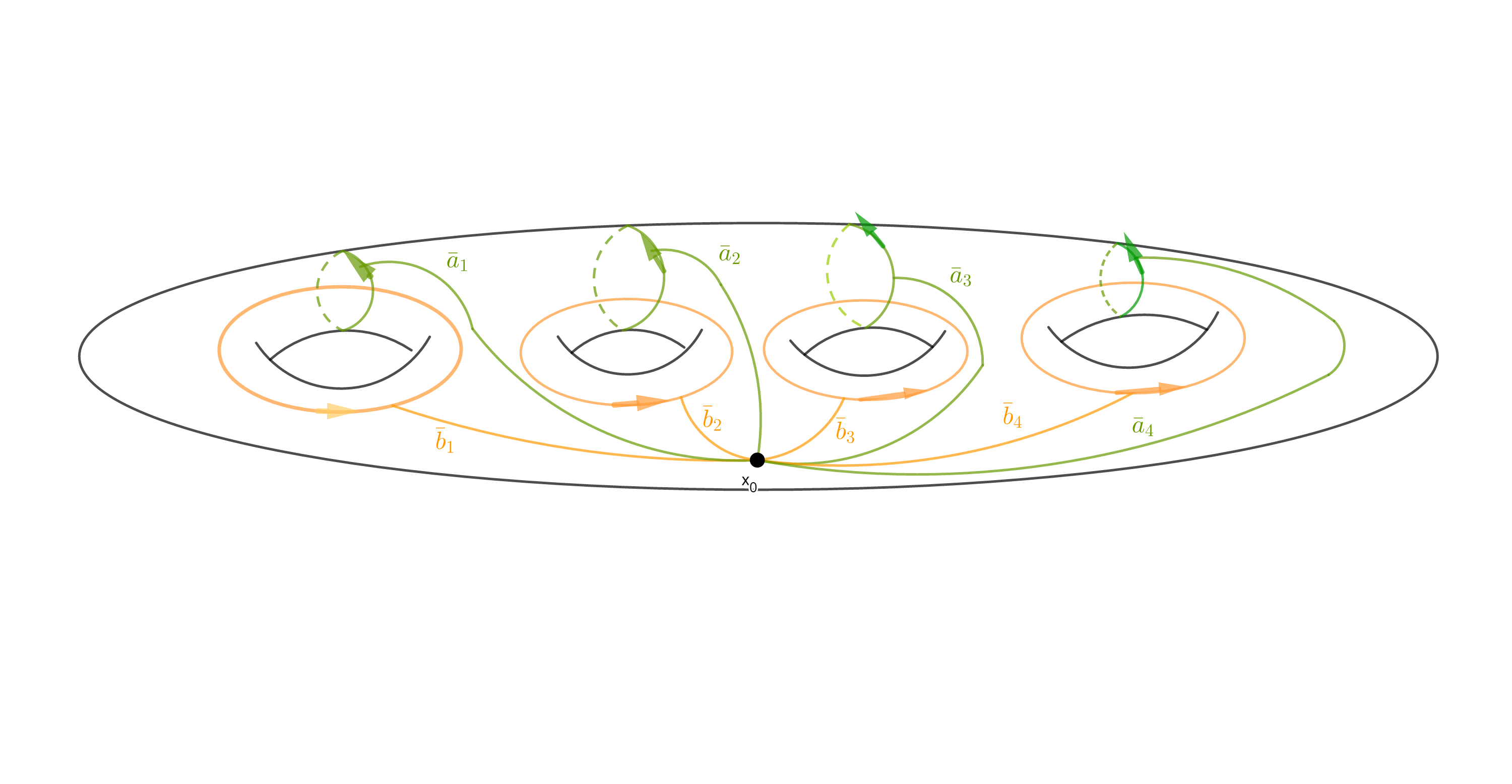
Figure 1. A collection of oriented loops $(\bar{a}_{1},\bar{b}_{1},\ldots,\bar{a}_{g},\bar{b}_{g})$ forming a symplectic basis in homology, here for $g=4$. The surface is considered has the boundary of an handlebody in $\mathbb{R}^{3}$ and the orientation of the surface is given by the normal vector pointing out the handlebody.

Let us now consider an element of $\mathfrak{G}_{n}$. We have seen two ways to describe it:

– either by some morphism $\sigma:\bar{\Gamma}\to\hat{\Gamma}_{n}$,

– or a map $\nu:\bar{\Gamma}\to\mathbb{Z}/n\mathbb{Z}$.

The link between the two is given by:

$$\forall\bar{\gamma}\in\bar{\Gamma}\;\;\sigma(\bar{\gamma})=\bar{\sigma}_{0}(\bar{\gamma})\bar{h}^{\nu(\bar{\gamma})}$$

For any element $\Gamma$ of $\mathfrak{G}_{n}$, the image under $[\bar{f}]$ of $\Gamma$ is the subgroup $[f]_{\ast}(\Gamma)$. It should be clear to the reader that if $\Gamma$ corresponds to the morphism $\sigma$, then $[f]_{\ast}(\Gamma)$ corresponds to the morphism $\sigma^{\prime}=[f]_{\ast}\circ\sigma\circ[\bar{f}]_{\ast}^{-1}$.

On the other hand, let denote by $\nu^{\prime}$ the map from $\bar{\Gamma}$ to $\mathbb{Z}/n\mathbb{Z}$ corresponding to $[f]_{\ast}(\Gamma)$. For any element $\bar{\gamma}$ of $\bar{\Gamma}$:

$$\bar{\sigma}_{0}(\bar{\gamma})\bar{h}^{\nu^{\prime}(\bar{\gamma})} = \sigma^{\prime}(\bar{\gamma})$$

$$= [f]_{\ast}(\sigma([\bar{f}]_{\ast}^{-1}(\bar{\gamma})))$$

$$= [f]_{\ast}(\bar{\sigma}_{0}([\bar{f}]_{\ast}^{-1}(\bar{\gamma}))\bar{h}^{\nu([\bar{f}]_{\ast}^{-1}(\bar{\gamma}))})$$

$$= [f]_{\ast}(\bar{\sigma}_{0}([\bar{f}]_{\ast}^{-1}(\bar{\gamma}))\bar{h}^{\nu([\bar{f}]_{\ast}^{-1}({\gamma}))}\;\mbox{since}\;[f]_{\ast}\;\mbox{is a morphism preserving}\;\bar{h}$$

$$= \bar{\sigma}_{0}(\bar{\gamma})\bar{h}^{\nu([\bar{f}]_{\ast}^{-1}(\bar{\gamma}))}\;\mbox{according to \eqref{eq:sigmaphi}}$$

Therefore, $\nu^{\prime}(\bar{\gamma})=\nu\circ[\bar{f}]_{\ast}^{-1}(\bar{\gamma})$. The Lemma is proved. ∎

Let us now fix a generator system of $\bar{\Gamma}$ satisfying the usual presentation:

$$\bar{\Gamma}=\langle\bar{a}_{i},\bar{b}_{i}\;(i=1,...,g)\>|\;[\bar{a}_{1},\bar{b}_{1}][\bar{a}_{2},\bar{b}_{2}]...[\bar{a}_{g},\bar{b}_{g}]=1\rangle$$

More precisely, we select a base point $x_{0}$, and take such a generator system so that every $\bar{a}_{i}$ and $\bar{b}_{i}$ is represented by a loop, such that the homology classes $[\bar{a}_{i}]$ and $[\bar{b}_{j}]$ form a symplectic basis for the intersection form (i.e. the intersection numbers $[\bar{a}_{i}].[\bar{a}_{j}]$ and $[\bar{b}_{i}].[\bar{b}_{j}]$ all vanish, and $[\bar{a}_{i}].[\bar{b}_{j}]$ as well except in the case $i=j$ where we have $[\bar{a}_{i}].[\bar{b}_{i}]=+1$). We furthermore require that the only intersection between any two such loops is reduced to the base point $x_{0}$. See Figure 1. Denote by $a_{i}$ and $b_{i}$ the images of $\bar{a}_{i}$ and $\bar{b}_{i}$ by ${\sigma}_{0}$, respectively.

Lemma 3.20 describes the way that $\operatorname{Mod}^{\pm}(\Sigma)$ acts on $\mathfrak{G}_{n}$, and we will now do the actual computation of this action. For this, we use the explicit generating system for $\operatorname{Mod}(\Sigma)$ provided by the Lickorish Theorem. Let $A_{i}$, $B_{i}$ and $C_{j}$ the simple closed curves depicted in Figure 2 ($1\leq i\leq g$, $1\leq j\leq g-1$).

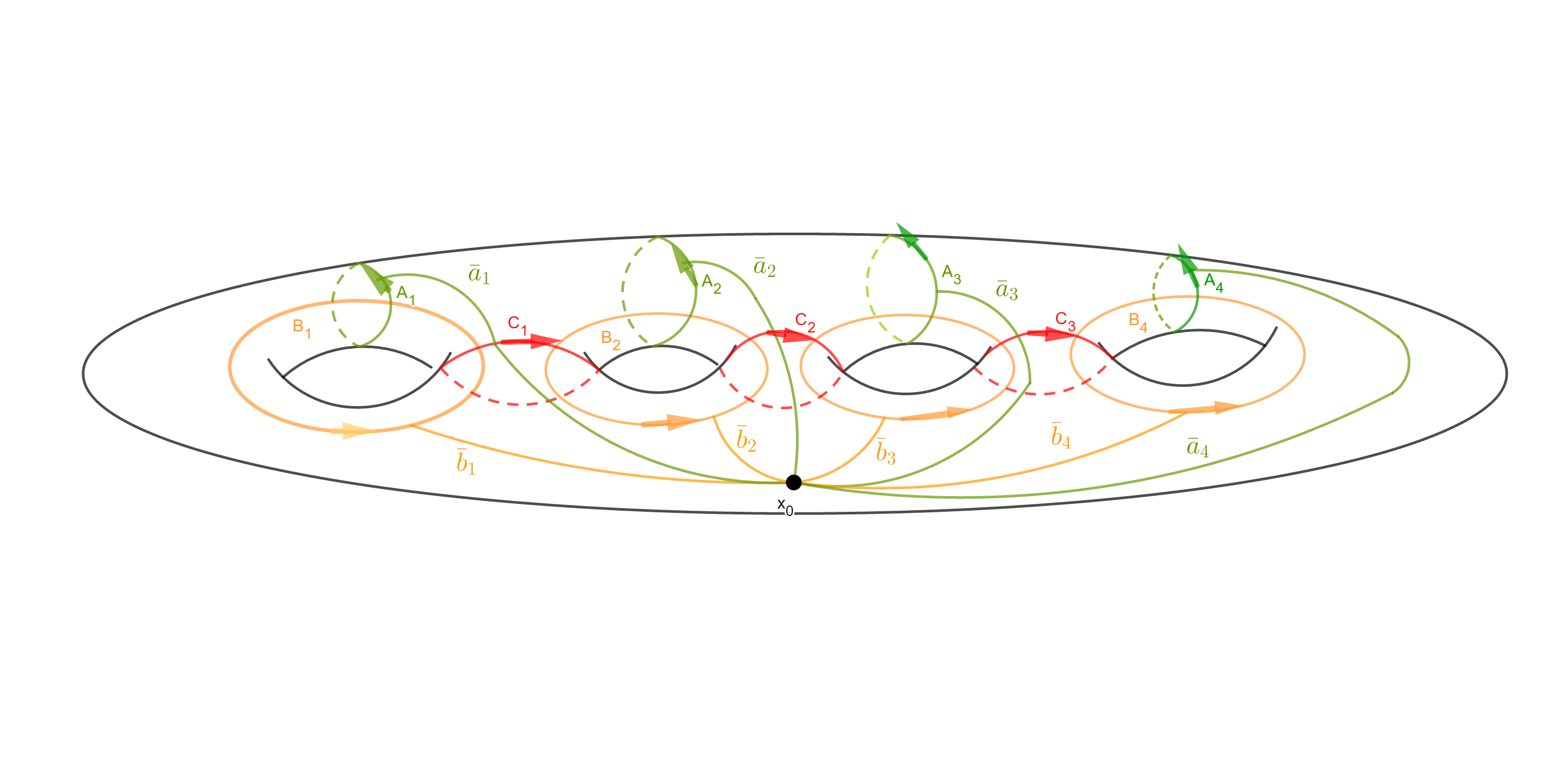
Figure 2. According to Lickorish’s Theorem, Dehn twists along these simple closed curves generate the mapping class group.

Theorem 3.21 (Lickorish [Lic]).

Let $(A_{1},B_{1},...,A_{g},B_{g},C_{1},\ldots,C_{g-1})$ the system of closed simple closed curves depicted in figure 2. Then, the Dehn twists along these curves generate $\operatorname{Mod}(\Sigma)$.

Slightly abusively, we will also denote by $A_{i}$, $B_{i}$ and $C_{j}$ the Dehn twists along these curves, and by $[A_{i}]_{\ast}$, $[B_{i}]_{\ast}$, $[C_{j}]_{\ast}$ the induced automorphisms of $\bar{\Gamma}\approx\pi_{1}(\Sigma,x_{0})$.

It follows from Figure 2 that for every $i$ between $1$ and $g$ that $[A_{i}]_{\ast}$ maps every generator $\bar{a}_{j}$ and $\bar{b}_{j}$ onto itself, except $\bar{b}_{i}$ for which we have:

$$[A_{i}]_{\ast}(\bar{b}_{i})=\bar{a}_{i}\bar{b}_{i}.$$

Therefore:

$$[A_{i}]^{-1}_{\ast}(\bar{b}_{i})=\bar{a}^{-1}_{i}\bar{b}_{i}.$$ (16)

Similarly $[B_{i}]_{\ast}$ maps every generator onto itself except $\bar{a}_{i}$ for which we have:

$$[B_{i}]_{\ast}(\bar{a}_{i})=\bar{a}_{i}\bar{b}^{-1}_{i}.$$

Hence:

$$[B_{i}]^{-1}_{\ast}(\bar{a}_{i})=\bar{a}_{i}\bar{b}_{i}.$$ (17)

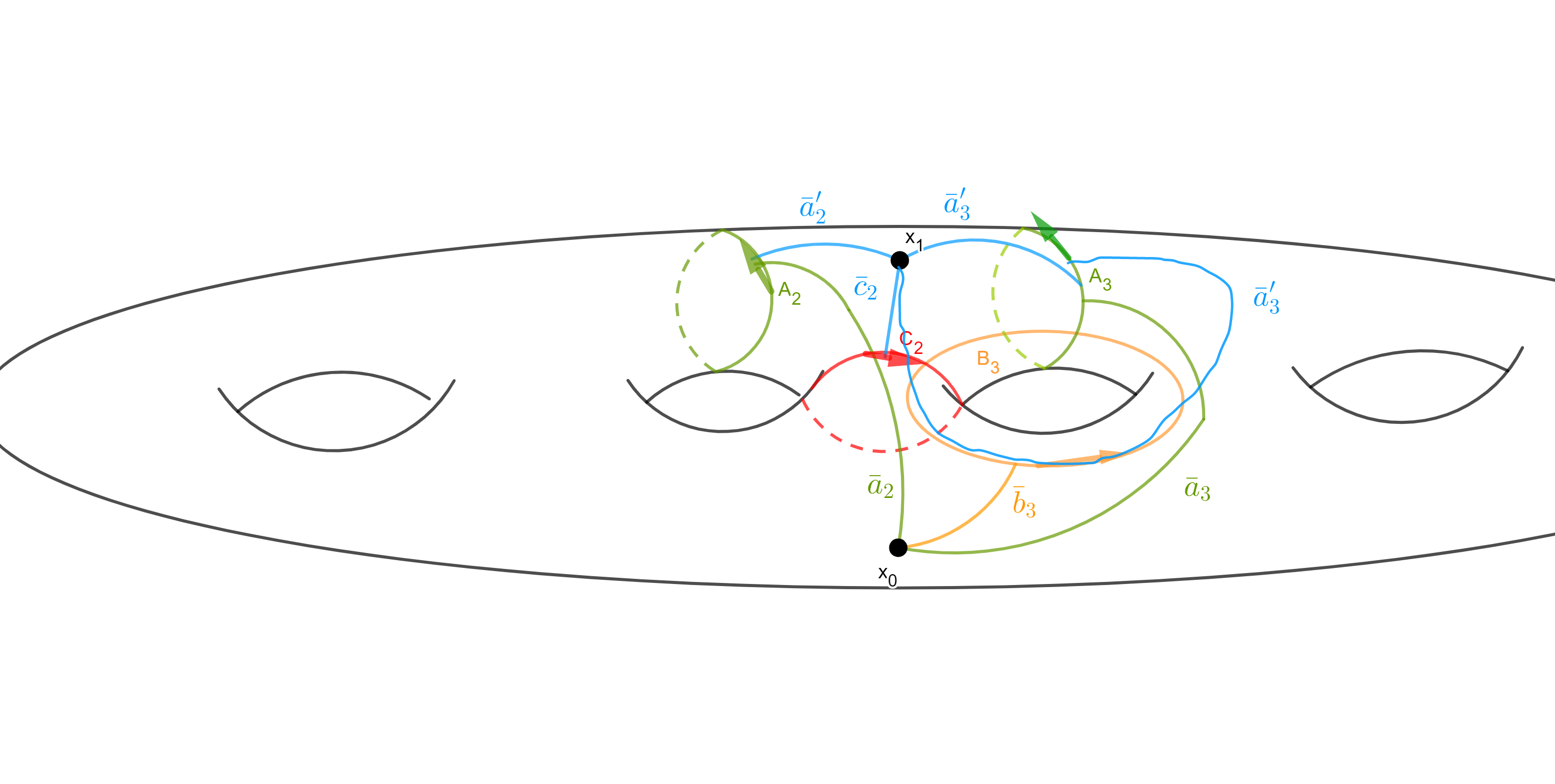
Figure 3. Definition of $\bar{a}^{\prime}_{3}$. Blue loops and green loops with the same label are homotopic.

The computation of the action of $[C_{i}]_{\ast}$ ($1\leq i\leq g-1$) is more intricate. Let $\bar{c}_{i}$ be the element of $\bar{\Gamma}$ defined by the loop describing first the initial part of $\bar{a}_{i}$ until it reaches $C_{i}$, then following $C_{i}$ in the direction depicted in Figure 2, then going back to $x_{0}$ by the path it uses to reach $C_{i}$. Then, $[C_{i}]_{\ast}$ acts trivially on every $\bar{a}_{j}$ for $j\neq i$, and also on every $\bar{b}_{j}$, except for $j=i$ and $j=i+1$. Furthermore:

$$[C_{i}]_{\ast}(\bar{a}_{i})=\bar{c}_{i}\bar{a}_{i}\bar{c}^{-1}_{i}$$

$$[C_{i}]_{\ast}(\bar{b}_{i})=\bar{c}_{i}\bar{b}_{i}$$

$$[C_{i}]_{\ast}(\bar{b}_{i+1})=\bar{b}_{i+1}\bar{c}^{-1}_{i}$$

Therefore, the inverse of $[C_{i}]_{\ast}$ satisfies:

$$[C_{i}]^{-1}_{\ast}(\bar{a}_{i})=\bar{c}^{-1}_{i}\bar{a}_{i}\bar{c}_{i},\;\;[C_{i}]^{-1}_{\ast}(\bar{b}_{i})=\bar{c}^{-1}_{i}\bar{b}_{i},\;\;[C_{i}]^{-1}_{\ast}(\bar{b}_{i+1})=\bar{b}_{i+1}\bar{c}_{i}.$$ (18)

Now we claim the following equality:

$$\bar{c}_{i}=\bar{a}_{i}\bar{b}_{i+1}\bar{a}_{i+1}^{-1}\bar{b}_{i+1}^{-1}$$ (19)

Indeed: let $a^{\prime}_{i+1}$ the loop based at the new base point $x_{1}$ in Figure 3. It follows from this picture that we have $\bar{c}_{i}=\bar{a}_{i}(\bar{a}^{\prime}_{i+1})^{-1}$. The same figure shows that we have:

$$\bar{a}_{i+1}=\bar{b}_{i+1}\bar{a}^{\prime}_{i+1}\bar{b}_{i+1}^{-1}$$

The equality (19) follows.

We can now compute how the generators $A_{i}$, $B_{i}$, $C_{i}$ acts on $\mathfrak{G}_{n}$.

Proposition 3.22.

Let $i$ be an integer between $1$ and $g$. The action of the element $[A_{i}]$ of $\operatorname{Mod}(\Sigma)$ represented by the Dehn twist $A_{i}$ on $\mathfrak{G}_{n}$ is given by:

$$[A_{i}]\ast\nu(\bar{a}_{j})=\nu(\bar{a}_{j})\ \ \forall j,\ \ \ [A_{i}]\ast\nu(\bar{b}_{j})=\nu(\bar{b}_{j})\ \ \forall j\neq i,\\ \ [A_{i}]\ast\nu(\bar{b}_{i})=-\nu(\bar{a}_{i})+\nu(\bar{b}_{i}).$$

The action of the element $[B_{i}]$ of $\operatorname{Mod}(\Sigma)$ represented by $B_{i}$ is:

$$[B_{i}]\ast\nu(\bar{b}_{j})=\nu(\bar{b}_{j})\ \ \forall j,\ \ \ [B_{i}]\ast\nu(\bar{a}_{j})=\nu(\bar{a}_{j})\ \ \forall j\neq i,\\ \ [B_{i}]\ast\nu(\bar{a}_{i})=\nu(\bar{a}_{i})+\nu(\bar{b}_{i}).$$

Finally, for $i$ between $1$ and $g-1$, the action of the element $[C_{i}]$ of $\operatorname{Mod}(\Sigma)$ represented by $C_{i}$ is:

$$[C_{i}]\ast\nu(\bar{a}_{j})=\nu(\bar{a}_{j})\ \ \forall j,\ \ \ [C_{i}]\ast\nu(\bar{b}_{j})=\nu(\bar{b}_{j})\ \ \forall j\neq i,i+1,$$

and

$$[C_{i}]\ast\nu(\bar{b}_{i})=\nu(\bar{b}_{i})-\nu(\bar{a}_{i})+\nu(\bar{a}_{i+1})+1,\;\;[C_{i}]\ast\nu(\bar{b}_{i+1})=\nu(\bar{b}_{i+1})+\nu(\bar{a}_{i})-\nu(\bar{a}_{i+1})-1$$

Proof.

Recall that according to Lemma 3.20, for every element $[\bar{f}]$ of $\operatorname{Mod}(\Sigma)$ we have:

$$[\bar{f}]\ast\nu=\nu\circ[\bar{f}]_{\ast}^{-1}.$$

Most formulae in the statement of the Proposition immediatly follow. The only cases we have to consider are:

$$[A_{i}]\ast\nu(\bar{b}_{i}) = \nu(\bar{a}_{i}^{-1}\bar{b}_{i})\;\;\mbox{(because of Equation \eqref{eq:calculA} )}$$

$$= -\nu(\bar{a}_{i})+\nu(\bar{b}_{i})-c(\bar{a}_{i}^{-1},\bar{b}_{i})\;\;\mbox{ (because of Equation \eqref{eq:nuc} )}$$

$$= -\nu(\bar{a}_{i})+\nu(\bar{b}_{i})\;\;\mbox{ (because of Lemma \ref{le:cvanishes} )}$$

The formula for $[B_{i}]\ast\nu(\bar{a}_{i})$ is similar.

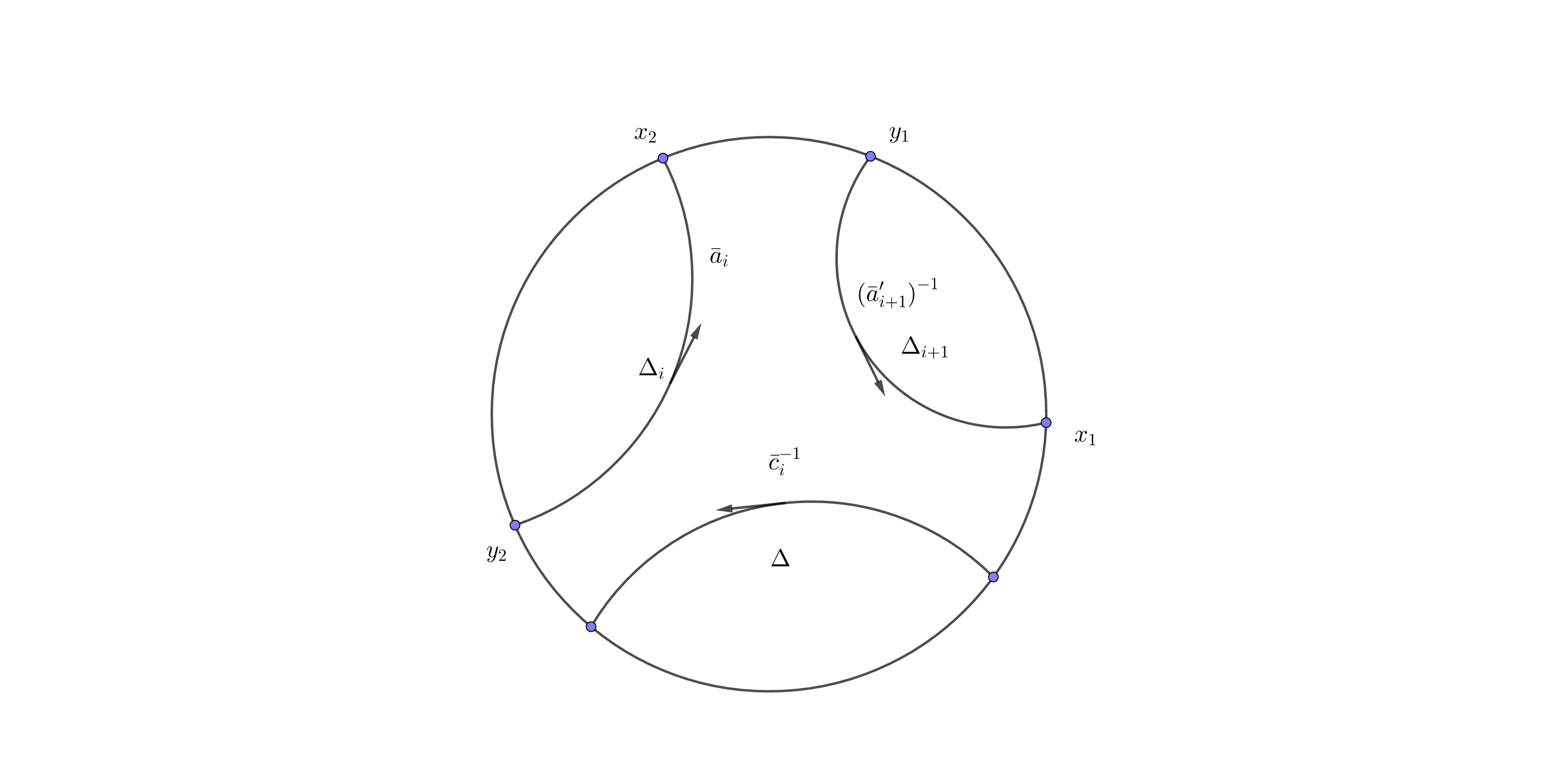
Figure 4. $\Delta$, $\Delta_{i}$ and $\Delta_{i+1}$ are preserved by respectively $\bar{c}^{-1}$, $\bar{a}_{i}$ and $(\bar{a}^{\prime}_{i+1})^{-1}$. The attracting fixed point of $(\bar{a}^{\prime}_{i+1})^{-1}$ is $x_{1}$, and the attracting fixed point of $\bar{a}_{i}$ is $x_{2}$.

The remaining computations we have to do are for $[C_{i}]_{\ast}\beta(\bar{a}_{i})$, $[C_{i}]_{\ast}\beta(\bar{b}_{i})$, and $[{C}_{i}]_{\ast}\beta(\bar{b}_{i+1})$. Concerning the first, we have:

$$[C_{i}]\ast\nu(\bar{a}_{i})=\nu(\bar{c}^{-1}_{i}\bar{a}_{i}\bar{c}_{i})=\nu(\bar{a}_{i})$$

Thanks to Equations (18), (12) one gets:

$$[C_{i}]\ast\nu(\bar{b}_{i})=\nu(\bar{b}_{i})-\nu(\bar{c}_{i})-c(\bar{c}_{i}^{-1},\bar{b}_{i}),\\ \ [C_{i}]\ast\nu(\bar{b}_{i+1})=\nu(\bar{b}_{i+1})+\nu(\bar{c}_{i})-c(\bar{b}_{i+1},\bar{c}_{i}).$$

But it follows from Lemma 3.2 that $c(\bar{c}_{i}^{-1},\bar{b}_{i})$ and $c(\bar{b}_{i+1},\bar{c}_{i})$ vanishes. Therefore:

$$[C_{i}]\ast\nu(\bar{b}_{i})=\nu(\bar{b}_{i})-\nu(\bar{c}_{i}),\;\;[C_{i}]\ast\nu(\bar{b}_{i+1})=\nu(\bar{b}_{i+1})+\nu(\bar{c}_{i})$$ (20)

Hence, the key point is to compute $\nu(\bar{c}_{i})$. Since $\bar{c}_{i}=\bar{a}_{i}(\bar{a}^{\prime}_{i+1})^{-1}$, we have:

$$\nu(\bar{c}_{i})=\nu(\bar{a}_{i})-\nu(\bar{a}^{\prime}_{i+1})-c(\bar{a}_{i},(\bar{a}^{\prime}_{i+1})^{-1})$$

Hence, we have to compute $c(\bar{a}_{i},(\bar{a}^{\prime}_{i+1})^{-1})$. Observe that the closed simple curves $A_{i}$, $C_{i}$ and $A_{i+1}$ form the boundary of a pair of pants. If we realize it as closed geodesics for the hyperbolic metric, we see that they are the projections of the axis of respectively $\bar{a}_{i}$, $\bar{c}_{i}$ and $(\bar{a}^{\prime}_{i+1})^{-1}$ (recall Figure 3). It follows that the axis of these elements in $\mathbb{H}^{2}$ have the configuration illustrated in Figure 4:

Consider now the lifted action in $\widetilde{\mathbb{R}P}^{1}$ is as in Figure 5. Here $a_{i}$ and $a^{\prime}_{i+1}$ are the lifts of $\bar{a}_{i}$ and $\bar{a}^{\prime}_{i+1}$ with fixed points in $\widetilde{\mathbb{R}P}^{1}$. Here $x_{2},y_{2}$ are fixed by $\bar{a}_{i}$ with $x_{2}$ the attracting fixed point. This generates $a_{i}$ fixing $\widetilde{x}_{2},\widetilde{y}_{2}$ (and infinitely many other pairs). Similarly $({a}^{\prime}_{i+1})^{-1}$ fixes $x_{1},y_{1}$ and so on.

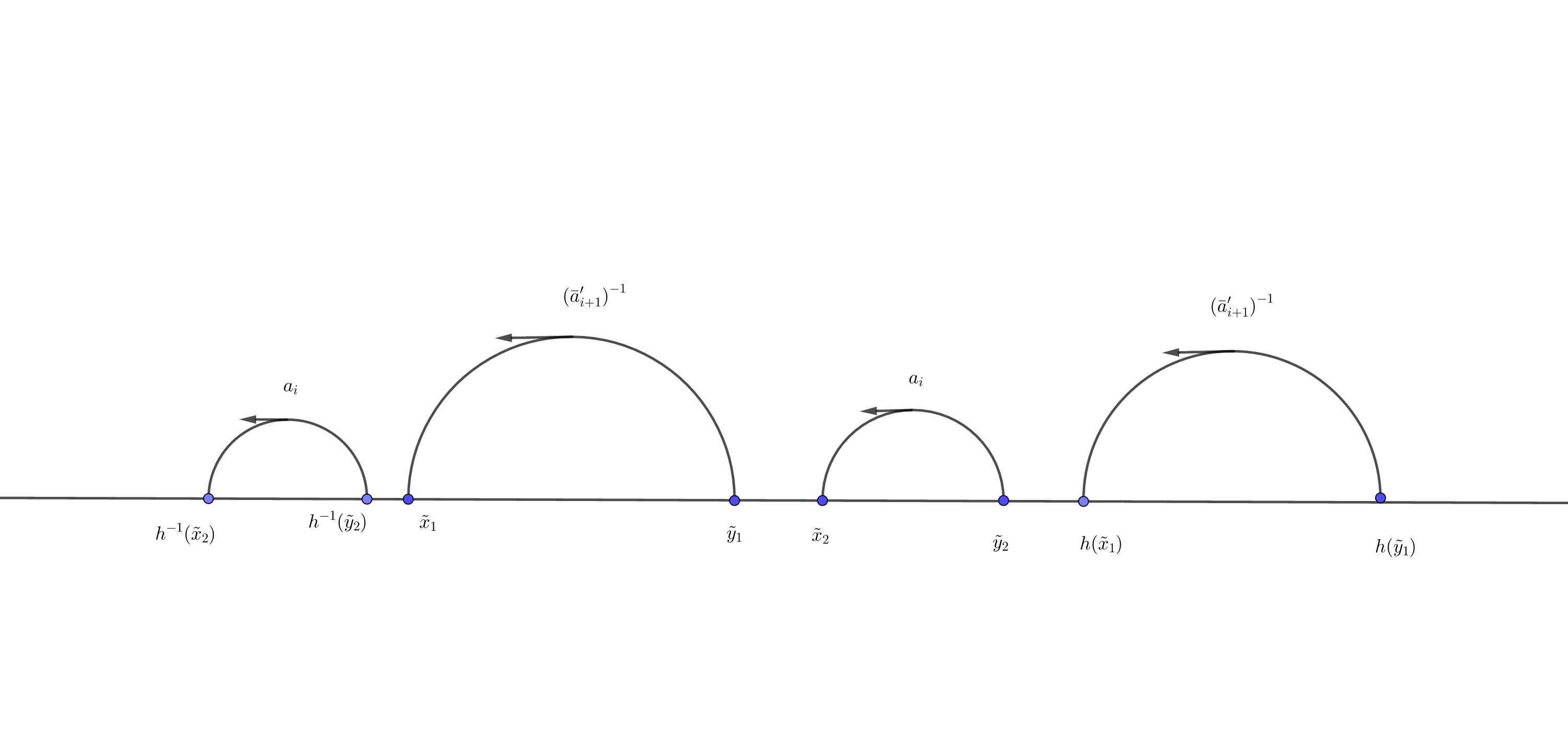
Figure 5. Liftings in $\widetilde{\mathbb{R}P}^{1}$. We have depicted two attracting fixed points $\tilde{x}_{1}$ and $h(\tilde{x}_{1})$ of $({a}^{\prime}_{i+1})^{-1}$, and two attracting fixed points $\tilde{x}_{2}$ and $h^{-1}(\tilde{x}_{2})$ of ${a}_{i}$.

Claim: for every $\tilde{x}$ in $\widetilde{\mathbb{R}P}^{1}$ we have $a_{i}(a^{\prime}_{i+1})^{-1}(\tilde{x})>\tilde{x}$.

Let us prove this claim. It is enough to prove it for every $\tilde{x}$ in the interval $[\tilde{y}_{1},h(\tilde{y}_{1})]$.

• If $\tilde{x}$ lies in $[\tilde{y}_{1},\tilde{x}_{2}]$: Then, we have $({a}^{\prime}_{i+1})^{-1}(\tilde{x})>\tilde{x}$. If $({a}^{\prime}_{i+1})^{-1}(\tilde{x})$ lies in $[\tilde{y}_{1},\tilde{x}_{2}]$, then its image by $a_{i}$ increases it, so the final image is bigger than $\tilde{x}$. If not, then $({a}^{\prime}_{i+1})^{-1}(\tilde{x})>\tilde{x}_{2}$, and therefore $a_{i}({a}^{\prime}_{i+1})^{-1}(\tilde{x})$ remains bigger than $\tilde{x}$. The Claim is true in this case.

• If $\tilde{x}$ lies in $[\tilde{x}_{2},\tilde{y}_{2}]$: The interval $[\tilde{x}_{2},\tilde{y}_{2}]$ is contained in the attracting region of $h(\tilde{x}_{1})$ under $(a^{\prime}_{i+1})^{-1}$ we therefore have $(a^{\prime}_{i+1})^{-1}(\tilde{x}_{2})>\tilde{x}_{2}$ and $(a^{\prime}_{i+1})^{-1}(\tilde{y}_{2})>\tilde{y}_{2}$. But since $\Delta_{i}$ is the lifting of a simple closed geodesic, $\tilde{y}_{2}$ cannot be between $a_{i}(\tilde{x}_{2})$ and $a_{i}(\tilde{y}_{2})$. Therefore, we have $(a^{\prime}_{i+1})^{-1}(\tilde{x}_{2})>\tilde{y}_{2}$: the interval $(a^{\prime}_{i+1})^{-1}([\tilde{x}_{2},\tilde{y}_{2}])$ is contained in the region $[\tilde{y}_{2},h(\tilde{x}_{1})]$ where we have $a_{i}(\tilde{x})>\tilde{x}$. Therefore, the Claim is still true there.

• If $\tilde{x}$ lies in $[\tilde{y}_{2},h(\tilde{x}_{1})]$: then $(a^{\prime}_{i+1})^{-1}(\tilde{x})$ lies in $[\tilde{x},h(\tilde{x}_{1})]$, and $a_{i}$ is increasing there, so the Claim is true in this case too.

• If $\tilde{x}$ lies in $[h(\tilde{x}_{1}),h(\tilde{y}_{1})]$: Then, $(a^{\prime}_{i+1})^{-1}(\tilde{x})$ remains in this interval. Therefore, its image under $a_{i}$ is bigger than $\tilde{x}$. The Claim follows once more since $a_{i}$ is increasing there.

The Claim is proved.

According to the Claim, the cocycle $c(\bar{a}_{i},(\bar{a}^{\prime}_{i+1})^{-1})$ is positive. In addition $a_{i}(\tilde{x}_{1})<h(\tilde{x}_{1})$, hence $c(\bar{a}_{i},(\bar{a}^{\prime}_{i+1})^{-1})\leq 1$. It follows $c(\bar{a}_{i},(\bar{a}^{\prime}_{i+1})^{-1})=1$.

Therefore:

$$\nu(\bar{c}_{i})=\nu(\bar{a}_{i})-\nu(\bar{a}^{\prime}_{i+1})-1$$

and since $\bar{a}^{\prime}_{i+1}$ is conjugated to $a_{i+1}$, we get:

$$\nu(\bar{c}_{i})=\nu(\bar{a}_{i})-\nu(\bar{a}_{i+1})-1$$

Equations (20) become:

$$[C_{i}]\ast\nu(\bar{b}_{i})=\nu(\bar{b}_{i})-\nu(\bar{a}_{i})+\nu(\bar{a}_{i+1})+1,\;\;[C_{i}]\ast\nu(\bar{b}_{i+1})=\nu(\bar{b}_{i+1})+\nu(\bar{a}_{i})-\nu(\bar{a}_{i+1})-1$$

The Proposition is proved. ∎

Equation (12) implies that the map $\nu:\bar{\Gamma}\to\mathbb{Z}/n\mathbb{Z}$ describing an element of $\mathfrak{G}_{n}$ is characterized by the values it takes on the generating set $\bar{a}_{i},\bar{b}_{i}\;(i=1,...,g)$. In other words, one can parametrize $\mathfrak{G}_{n}$ by the $n$-tuples $(\alpha_{1},\beta_{1},\ldots,\alpha_{g},\beta_{g})$ in $(\mathbb{Z}/n\mathbb{Z})^{2g}$ where $\alpha_{i}$ is the value taken by $\nu$ at $\bar{a}_{i}$, and $\beta_{i}$ the value it takes at $\bar{b}_{i}$. Observe that all values are possible since one can add to any $\nu$ any morphism from $\bar{\Gamma}$ into $\mathbb{Z}/n\mathbb{Z}$.

Let us decompose $\mathfrak{G}_{n}$ as a sum $V_{1}\oplus\ldots\oplus V_{g}$ where every $V_{i}$ is made of elements with coordinates $(\alpha_{1},\beta_{1},\ldots,\alpha_{g},\beta_{g})$ satisfying $\alpha_{j}=\beta_{j}=0$ for all $j\neq i$. According to Proposition 3.22, this decomposition is invariant by the subgroup $G$ of $\operatorname{Mod}(\Sigma)$ generated by the $[A_{i}]$’s and the $[B_{i}]$’s. More precisely, in every $V_{i}$, the actions of $[A_{i}]$ and $[B_{i}]$ are given by the matrices:

$$\left(\begin{array}[]{cc}1&0\\ -1&1\\ \end{array}\right)\quad\left(\begin{array}[]{cc}1&1\\ 0&1\\ \end{array}\right)$$

In particular, the action of $G$ preserves $(0,...,0)$: it is linear. Moreover, these two matrices generate the entire SL$(2,\mathbb{Z}/n\mathbb{Z})$, therefore, any element of SL$(2,\mathbb{Z}/n\mathbb{Z})^{g}$ is realized by an element of $G$.

On the other hand, Proposition 3.22 shows that for every $i$ between $1$ and $g-1$, the action of $[C_{i}]$ is trivial on $V_{j}$ for $j\neq i,i+1$, and that on $V_{i}\oplus V_{i+1}$ this action is given by:

$$\left(\begin{array}[]{ccccc}1&0&0&0&|0\\ -1&1&1&0&|1\\ 0&0&1&0&|0\\ 1&0&-1&1&|-1\end{array}\right)$$

This action is not linear, and its translation part $\tau([C_{i}]_{\ast})$ (see Remark 3.18) in the coordinate system $(\alpha_{1},\beta_{1},\ldots,\alpha_{g},\beta_{g})$ is the vector satisfying $\beta_{i}=-\beta_{i+1}=1$, with all other coordinates vanishing.

We can now prove our Main Theorem:

Theorem 3.23.

Let $q_{0}:M\to M_{1}(\Sigma)$ be a finite covering of index $n$ along the fibers. Then, if $n$ is odd, there is only one Anosov flow on $M$ up to orbital equivalence. If $n$ is even, there are two orbital equivalence classes of Anosov flows.

Proof.

Since any element of SL$(2,\mathbb{Z}/n\mathbb{Z})^{g}$ is realized by an element of $G$, every element of $\mathfrak{G}_{n}$ admits in its $G$-orbit an element of the form:

$$(0,\beta_{1},0,\beta_{2},\ldots,0,\beta_{g})$$ (21)

Let us now consider the subgroup $\mathfrak{C}$ generated by the $g-1$ elements $C_{1},\ldots,C_{g-1}$. Since all the curves $\bar{c}_{i}$ are disjoint, it is an abelian group. The action of some element $C_{1}^{k_{1}}C_{2}^{k_{2}}\ldots{C}_{g-1}^{k_{g-1}}$ is:

$$\alpha_{i} \to \alpha_{i}$$

$$\beta_{i} \to \beta_{i}+k_{i}\alpha_{i+1}-(k_{i}+k_{i-1})\alpha_{i}+k_{i-1}\alpha_{i-1}+k_{i}-k_{i-1}$$

where we adopt the convention $k_{0}=k_{g}=0$. This action does not change the value of each $\alpha_{i}$, and moreover one can check that the sum $\sum_{i=1}^{g}\beta_{i}$ is constant along the orbits of $\mathfrak{C}$. We do not do an explicit computation here. Anyway, we see that by applying a well-suited element of $\mathfrak{C}$, we can transform the element of the form (21) to another one where all the $\alpha_{i}$’s and $\beta_{i}$’s vanish, except $\beta_{g}$. In other words, every element of $\mathfrak{G}_{n}$ admits in its $\operatorname{Mod}(\Sigma)$-orbit an element of the form:

$$(0,0,\ldots,0,0,0,\beta)$$ (22)

Let us go back, applying $C_{g-1}$, we get:

$$(0,0,\ldots,0,1,0,\beta-1)$$

Now use an element of $G$ mapping this element to:

$$(0,0,\ldots,0,1,\beta-1,0)$$

Apply $C_{g-1}$: we now get:

$$(0,0,\ldots,0,\beta+1,\beta-1,-\beta)$$

Since $\beta-1$ and $-\beta$ are relatively prime, applying an element of $G$, composition of $A_{g}$’s and $B_{g}$’s, we obtain:

$$(0,0,\ldots,0,\beta+1,0,1)$$

and by applying $C_{g-1}^{-1-\beta}$, we get:

$$(0,0,\ldots,0,0,0,\beta+2)$$

In summary, any element of $\mathfrak{G}_{n}$ admits in its $\operatorname{Mod}(\Sigma)$-orbit an element of the form $(0,0,\ldots,0,0,0,\beta)$, and admits also all the elements of the form $(0,0,\ldots,0,0,0,\beta+2k)$ where $k$ is any integer.

It follows that when $n$ is odd, in which case $2$ is a generator of $\mathbb{Z}/n\mathbb{Z}$, that every $\operatorname{Mod}(\Sigma)$-orbit in $\mathfrak{G}_{n}$ contains $(0,0,\ldots,0,0,0,0)$. In other words, there is only one $\operatorname{Mod}(\Sigma)$-orbit; hence only one $\operatorname{Mod}^{\pm}(\Sigma)$-orbit. The theorem follows in this case from Proposition 3.19.

Let us now assume that $n$ is even. The same argument as above shows that there are at most two $\operatorname{Mod}(\Sigma)$-orbits in $\mathfrak{G}_{n}$: the orbit of $(0,0,\ldots,0,0,0,0)$ and the orbit of $(0,0,\ldots,0,0,0,1)$. The proof of the Theorem will be finished if we prove that these two orbits are disjoint.

Since $n$ is even, every $\alpha_{i}$ and $\beta_{i}$, which is an integer modulo $n$, defines an element $\bar{\alpha}_{i}$ and $\bar{\beta}_{i}$ of $\mathbb{Z}/2\mathbb{Z}$. In other words, there is a well-defined map $\mathfrak{G}_{n}\to\mathfrak{G}_{2}$. This map is clearly $\operatorname{Mod}^{\pm}(\Sigma)$-equivariant, therefore, if the $\operatorname{Mod}^{\pm}(\Sigma)$-orbits of $(0,0,\ldots,0,0,0,0)$ and of $(0,0,\ldots,0,0,0,1)$ are different in $\mathfrak{G}_{2}$, there are also different in $\mathfrak{G}_{n}$.

Hence, in order to achieve the proof of the Theorem, we just have to consider the case $n=2$.

For every element of $\mathfrak{G}_{2}=V_{1}\oplus\ldots\oplus V_{g}$, let us call vanishing number the number of indices $i$ for which the components in $V_{i}$ are zero. More precisely, the vanishing number is this integer modulo $2$. For example, the vanishing number for $(0,0,\ldots,0,0,0,0)$ is the class modulo $2$ of $g$, whereas the vanishing number for $(0,0,\ldots,0,0,0,1)$ is the class modulo $2$ of $g-1$: they are different.

Claim: The vanishing number is constant along $\operatorname{Mod}(\Sigma)$-orbits.

Let us prove the claim: clearly, the vanishing number does not change under the action of $A_{i}$ or $B_{i}$, since they act in $V_{i}$ as elements of SL$(2,\mathbb{Z}/2\mathbb{Z})$.

Let us consider $C_{i}$ ($1\leq i\leq g-1$). It acts trivially on every $V_{j}$ except maybe $V_{i}$ and $V_{i+1}$.

– If $\alpha_{i}=\alpha_{i+1}=1$, the components in $V_{i}$ and $V_{i+1}$ are nonzero, and the same is true after applying $C_{i}$ since we still have after the action $\alpha_{i}=\alpha_{i+1}=1$: the vanishing number remains the same.

– If $\alpha_{i}\neq\alpha_{i+1}$, then, since we are in $\mathbb{Z}/2\mathbb{Z}$, we have $\alpha_{i+1}-\alpha_{i}+1=0$, and it follows that $C_{i}$ acts trivially on such an element: the vanishing number remains the same in this case too.

– If $\alpha_{i}=\alpha_{i+1}=0$: then we have:

$$C_{i}(0,\beta_{i},0,\beta_{i+1})=(0,\beta_{i}+1,0,\beta_{i+1}+1)$$

Hence, if $\beta_{i}=\beta_{i+1}=0$, or if $\beta_{i}=\beta_{i+1}=1$, the vanishing number before and after $C_{i}$ differ by $2$, hence is the same modulo $2$. If $\beta_{i}\neq\beta_{i+1}$, one component vanishes and not the other, and the same is true after applying $C_{i}$.

We have proved the Claim. Since the vanishing numbers of $(0,0,\ldots,0,0,0,0)$ and $(0,0,\ldots,0,0,0,1)$ are different, they cannot be in the same $\operatorname{Mod}(\Sigma)$-orbit.

The only remaining step is to show that the vanishing number is also preserved by orientation reversing elements of $\operatorname{Mod}^{\pm}(\Sigma)$. For this, we just have to prove that it is true for one of them. Let us consider the symetry $s$ in the horizontal plane containing all the simple closed curves $B_{i}$ (see Figure 2). One can assume, and we do, that the base point $x_{0}$ is fixed by $s$. Then, every loop $a_{i}$ is mapped to a loop conjugated to its inverse. In addition every loop $\bar{b}_{i}$ is taken to a loop conjugated to itself. Therefore, the action of $[s]$ on $\mathfrak{G}_{2}$ (or $\mathfrak{G}_{n}$) is simply, for all $j$:

$$[s]\ast\beta(a_{j})=-\beta(a_{j})$$

$$[s]\ast\beta(b_{j})=\beta(b_{j})$$

This obviously preserves the vanishing number. Thus concludes the proof of Theorem 3.23. ∎

We end this Section with a proposition showing that the image in Aff$(\mathfrak{G}_{n})$ of $\operatorname{Mod}(\Sigma)$ is isomorphic to Sp$(2g,\mathbb{Z}/n\mathbb{Z})$.

Proposition 3.24.

The Torelli group acts trivially on $\mathfrak{G}_{n}$.

Proof.

By definition, an element of the Torelli group is an element of $\operatorname{Mod}(\Sigma)$ which acts trivially in homology. In particular it is orientation preserving. It follows that its linear part as defined in Remark 3.18 is the identity. But it could still act on $\mathfrak{G}_{n}$ as a translation. However, by a Theorem of Johnson ([Joh]) combined with a Theorem of Powell in the case $g=2$ ([Pow]), the Torelli group is generated by:

– Dehn twists along separating non-homotopically trivial simple closed curves in the case $g=2$,

– compositions $T_{1}T_{2}^{-1}$ where $T_{1}$ and $T_{2}$ are left Dehn twists along simple closed curves that are boundary of a compact surface of genus $1$ embedded in $\Sigma$ (in the case $g\geq 3$).

Consider the red simple closed curves $D_{1},\ldots,D_{g-1}$ depicted in Figure 6. They are disjoint from the curves $A_{i}$ and $B_{i}$, therefore the Dehn twists along $D_{1},\ldots,D_{g-1}$ preserves the conjugacy classes of $\bar{a}_{i}$ and $\bar{b}_{i}$. It follows that their action on $\mathfrak{G}_{n}$ is trivial.

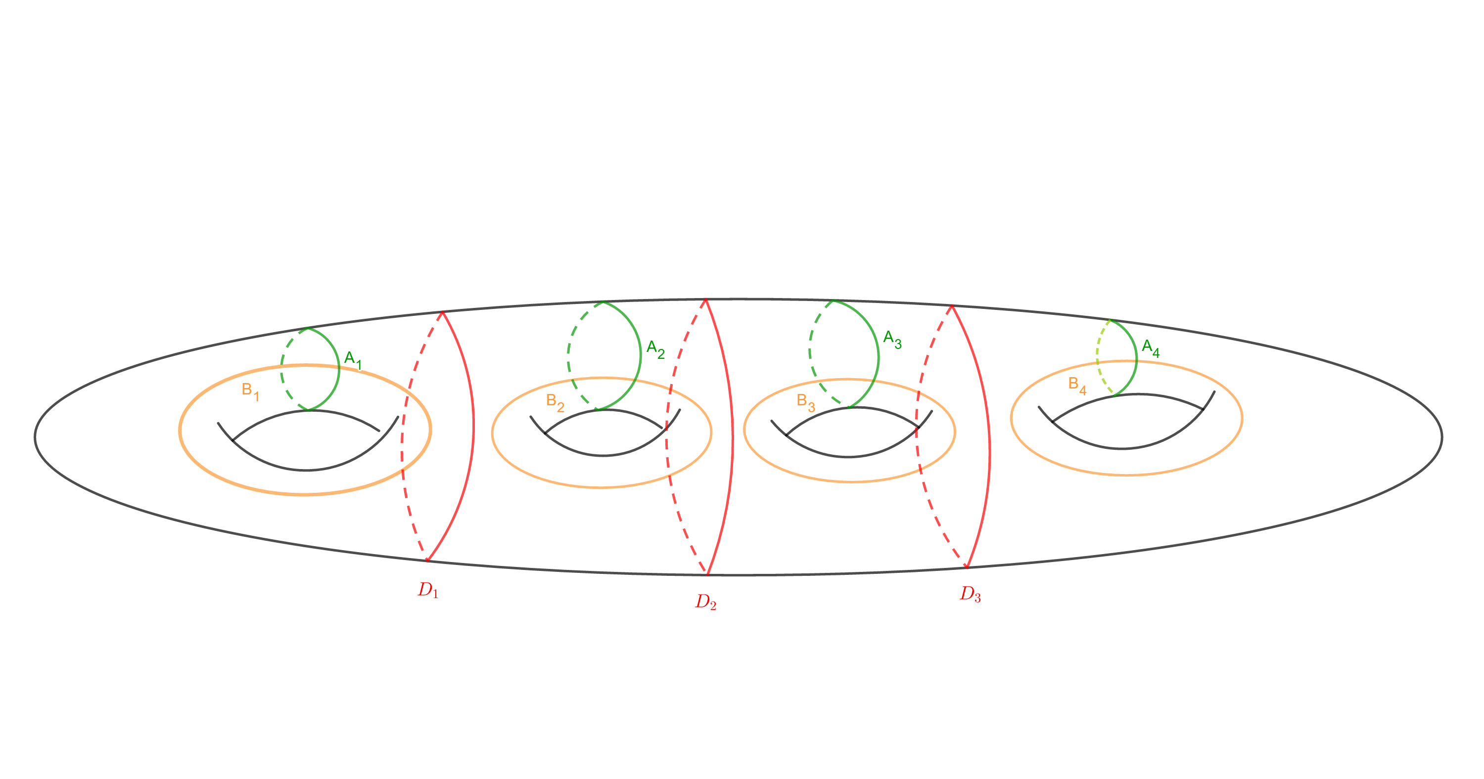
Figure 6. $g-1$ non separating curves on the surface.

But, in the case $g=2$, there is only one such a curve $D_{1}$, and every separating, homotopically non-trivial simple closed curve in $\Sigma$ is the image of $D_{1}$ under some homeomorphism. The proposition follows in this case since the kernel of the action is a normal subgroup of $\operatorname{Mod}(\Sigma)$.

The case $g\geq 3$ is similar and comes from the fact that any pair of simple closed curves bounding a genus $1$ surface embedded in $\Sigma$ is the image under some homeomorphism of two successive loops $D_{i}$ and $D_{i+1}$. ∎

Remark 3.25.

According to proposition 3.24, the action of $\operatorname{Mod}(\Sigma)$ on $\mathfrak{G}_{n}$ induces a (faithful) affine action of Sp$(2g,\mathbb{Z}/n\mathbb{Z})$ on the torus $\mathfrak{G}_{n}\approx(\mathbb{Z}/n\mathbb{Z})^{2g}$ whose linear part is the canonical representation of Sp$(2g,\mathbb{Z}/n\mathbb{Z})$. But this action is affine and admits a non-trivial translation part $[\tau]$, that represents a non-trivial element of $H^{1}(\operatorname{Sp}(2g,\mathbb{Z}/n\mathbb{Z}),(\mathbb{Z}/n\mathbb{Z})^{2g})$.

This feature is in contrast with the fact that $H^{1}(\operatorname{Sp}(2g,\mathbb{Z}),(\mathbb{Z})^{2g})$ vanishes (every affine action of $\operatorname{Sp}(2g,\mathbb{R})$ has a global fixed point, since every linear representation splits as a sum of irreducible representations).

Remark 3.26.

In [Gi], E. Giroux considered a related problem: the classification of contact structures on the circle bundle $M$ up to isotopy and up to conjugation by a diffeomorphism. A case of interest for us is the case of universally tight contact structures, with wrapping number $-n$. E. Giroux shows that they are all isotopic to the pull-back $q^{\ast}\alpha_{0}$ by some finite covering $q:M\to M_{1}(\Sigma)$ along the fibers, where $\alpha_{0}$ is the contact $1$-form on $M_{1}(\Sigma)$ whose Reeb flow is the geodesic flow (for some hyperbolic Riemannian metric). According to Ghys’ Theorem (see Theorem 2.9), Anosov flows on $M$ are always isotopic to the Reeb flow of such a structure. Clearly, an isotopy between contact structures provides an isotopy between their Reeb flows, i.e. Anosov flows, and vice-versa. Similarly, there is a one-to-one correspondence between conjugacy classes of these contact structures and orbital equivalence classes of Anosov foliations.

As a matter of fact, Giroux obtains a classification of isotopy classes similar as we do here: the action of $K_{1}$ on these contact structures is freely transitive. Actually, it follows from Giroux’s work and the results in the present paper that these two classification problems are equivalent.

He furthermore claims to have classified conjugacy classes, and to show that the number of conjugacy classes of these contact structures is the number $\varphi(n)$ of divisors of $n$ ([Gi, Theorem $3.1$ and Proposition $3.10$]). Hence, this statement is in contradiction with our Theorem 3.23.

The point is that Giroux’s proof is not completely correct at this concluding step: in the proof of Proposition $3.10$, he implicitly assumes that the action of $\operatorname{Mod}(\Sigma)$ on the space $\mathfrak{G}_{n}$ of index $n$ subgroups along the fiber is linear, whereas this action is genuinely affine, as shown in the present article.

References

- [1]
- [An] D. V. Anosov, Geodesic flows on closed Riemannian manifolds with negative curvature, Proc. Steklov Inst. Math. 90 (1969).
- [Ba1] T. Barbot, Caractérisation des flots d’Anosov en dimension par leurs feuilletages faibles, Ergod. Th. Dynam. Sys. 15 (1995) 247-270.
- [Ba2] T. Barbot, Flots d’Anosov sur les variétés graphées au sens de Waldhausen, Ann. Inst. Fourier Grenoble 46 (1996) 1451-1517.
- [Ba3] T. Barbot, Plane affine geometry of Anosov flows, Ann. Sci. Ecole Norm. Sup. 34 (2001) 871-889.
- [Fa-Ma] B. Farb, D. Margalit, A primer on mapping class groups, Princeton Mathematical Series 49 (2012).
- [Fen] S. Fenley, Anosov flows in -manifolds, Ann. of Math. 139 (1994) 79-115.
- [Fe-Mo] S. Fenley and L. Mosher, Quasigeodesic flows in hyperbolic -manifolds, Topology 40 (2001) 503-537.
- [Gh1] E. Ghys, Flots d’Anosov sur les -variétés fibrées en cercles, Ergod. Th and Dynam. Sys. 4 (1984) 67-80.
- [Gh2] E. Ghys, Groupes d’homéomorphismes du cercle et cohomologie bornée, Contemporary Mathematics 58 (1987) 81-106.
- [Gh3] E. Ghys, Groups acting on the circle, Enseign. Math. (2) 47 (2001) 329–407.
- [Gi] E. Giroux, Structures de contact sur les variétés fibrées en cercles au-dessus d’une surface, Comm. Math. Helv. 76 (2001) 218–262.
- [Gro] M. Gromov, Three remarks on geodesic dynamics and fundamental group, Enseign. Math. (1) 46 (2000) 391–402
- [Ha-Ka] B. Hasselblatt and A. Katok, Introduction to the modern theory of duynamical systems, Cambridge Univ. Press, 1995.
- [Hu-Ka] S. Hurder, A. Katok, Differentiability, rigidity and Godbillon-Vey classes for Anosov flows, Inst. Hautes Études Sci. Publ. Math. 72 (1990), 5-61.
- [Joh] D.L. Johnson, Homeomorphisms of a surface which act trivially on homology, Proc. Amer. Soc., 75 (1979) 119–125.
- [Lic] W. B. R. Lickorish, A finite set of generators for the homeotopy group of a -manifold, Proc. Cambridge Philos. Soc., 60 (1964) 769–778.
- [Pow] J. Powell, Two theorems on the mapping class group of a surface, Proc. Amer. Soc., 68 (1978) 347–350.
- [Rand] O. Randal-Williams, Homology of the moduli spaces and mapping class groups of framed, -Spin and Pin surfaces, J. Topol., 7 (2014), no. 1, 155–186.
- [Sou] J. Souto, A remark on the action of the mapping class group on the unit tangent bundle, Ann. Fac. Sci. Toulouse Math. 19 (2010) 589-601.
- [Wald] F. Waldhausen, On irreducible -manifolds which are sufficiently large, Ann. of Math. 87 (1968) 56-88.