ChASE - A Distributed Hybrid CPU-GPU Eigensolver for Large-scale Hermitian Eigenvalue Problems

Abstract.

As modern massively parallel clusters are getting larger with beefier compute nodes, traditional parallel eigensolvers, such as direct solvers, struggle keeping the pace with the hardware evolution and being able to scale efficiently due to additional layers of communication and synchronization. This difficulty is especially important when porting traditional libraries to heterogeneous computing architectures equipped with accelerators, such as Graphics Processing Unit (GPU). Recently, there have been significant scientific contributions to the development of filter-based subspace eigensolver to compute partial eigenspectrum. The simpler structure of these type of algorithms makes for them easier to avoid the communication and synchronization bottlenecks typical of direct solvers. The Chebyshev Accelerated Subspace Eigensolver (ChASE) is a modern subspace eigensolver to compute partial extremal eigenpairs of large-scale Hermitian eigenproblems with the acceleration of a filter based on Chebyshev polynomials. In this work, we extend our previous work on ChASE by adding support for distributed hybrid CPU-multi-GPU computing architectures. Out tests show that ChASE achieves very good scaling performance up to 144 nodes with 526 NVIDIA A100 GPUs in total on dense eigenproblems of size up to $360$k.

1. Introduction

Modern scientific and engineering applications (e.g., in the filed of electronic structure in condensed matter physics (Kohn and Sham, 1965; Becke, 1993; Kohn, 1999)) often require the solution of very large dense eigenproblems distributed on massive supercomputers. In the last decades, there have been continuous efforts to develop efficient parallel eigensolver libraries for large dense matrices targeted at systems with a large number of compute nodes (Choi et al., 2003; Poulson et al., 2013; ELPA, 2014; Imamura et al., 2011). Dense eigensolvers, even those for extremal eigenproblems in which only a fraction at the end of the spectrum is sought after, have $\mathcal{O}(n^{3})$ complexity. Unlike simpler linear algebra operations, eigensolvers consist of several "moving parts", many of which can differ significantly in terms of computational intensity. Because of these characteristics, it is often challenging to construct parallel implementations of dense eigensolvers that scale well on large supercomputers, and ensure a good balance between different nodes throughout the computation. When it comes to efficiently porting dense eigensolvers to distributed GPGPU (General Purpose GPU) systems, this challenge becomes even harder to address. Currently, only the ELPA library (ELPA, 2014; Yu et al., 2021) carried out such an endeavor with moderate success. To our knowledge, no library is able to successfully exploit GPUs for very large dense eigenproblems with size larger than 100k.

The lack of balanced scalability on heterogeneous platforms is an important issue in light of the current trend towards massively parallel clusters trying to reach exascale. To grasp this target, future architectures will have to leverage compute nodes equipped with beefy multi-core CPUs coupled with powerful multi-GPUs via a high-bandwidth interconnect (e.g. the NVIDIA Grace project (NVIDIA, 2021)). Having a dense eigensolver running efficiently on such architectures is paramount. In order to develop efficient distributed multi-GPU eigensolver libraries, the implementations should be designed with a large amount of concurrency and a minimal data transfer between host and device memory.

To address this problem, we propose a distributed hybrid CPU-GPU version of the ChASE eigensolver. ChASE, short for Chebyshev Accelerated Subspace iteration Eigensolver, is a modern library based on subspace iteration accelerated with a Chebyshev polynomial filter and includes some innovative algorithmic features (Berljafa et al., 2015; Winkelmann et al., 2019). It is designed to approximate extremal eigenpairs of dense symmetric and Hermitian matrices and is particularly effective in solving sequences of correlated eigenproblems (e.g., derived by the linearization of non-linear problems). An MPI-based parallel implementation of ChASE for homogeneous systems has already been presented in (Winkelmann et al., 2019), and will be referred to as ChASE-CPU. We have referred to the hybrid CPU-GPU implementation presented in this paper as ChASE-GPU.

Due to its algorithm design, ChASE is able to scale well on distributed multi-GPU clusters. As shown in (Winkelmann et al., 2019), the algorithm can be decoupled in a series of basic linear operations, the most important of which is the Hermitian Matrix-Matrix Multiplications (HEMMs) repeatedly executed within the Chebyshev polynomial Filter. As a typical BLAS-3 operation, the performance of an efficient implementation of the distributed HEMM is able to approach the theoretical peak performance of a given system. Other linear algebra operations are computed redundantly on each MPI process, minimizing the inter-node communication. We provide the hybrid CPU-GPU implementation of ChASE by designing and implementing a customized distributed HEMM that supports flexible configurations of binding MPI processes and GPUs within the compute node. In addition, selected computationally intensive linear algebra operations, such as QR factorization, are also offloaded to one of the GPUs tied to each MPI process. Because to the relatively small memory capacity of the device, we provide accurate formulas for estimating the memory cost for CPU and GPU to help the user choose the optimal resource usage for a given problem. ChASE-GPU has been tested on our in-house supercomputer JURECA Data Centric Module (JURECA-DC). The strong scaling tests were performed with a symmetric matrix of size 130k with double-precision using up to 64 compute nodes and with a total of 256 NVIDIA A100 GPUs. Similarly, the weak scaling test was performed using up to 144 compute nodes with a total of 576 GPUs, using symmetric matrices ranging in size from 30k to 360k. We have also performed a strong scaling test up to 64 compute nodes comparing ChASE-GPU with ELPA2 with GPU support. This last test was carried out on an Hermitian eigenproblem of size 76k generated by the discretization of the Bethe-Salpeter equation used to simulate the opto-electronic properties of In₂O₃.

Original contributions. We have significantly improved the performance of the existing custom-HEMM, which is mainly tailored to the execution of the 3-terms recurrence relation at the base of the polynomial Filter. Although ChASE-CPU already supported GPUs, it could only use a single GPU per MPI rank. We increased the flexibility of the custom-HEMM by extending support for multiple GPUs per MPI rank. We achieved this result by adding a further custom distribution of the data to allow the execution of multi-GPU HEMM operations local to each MPI rank. We also optimized the design of the filter by removing redundancies in the code and reducing the memory footprint of the algorithm. As a result we gained an increased scalability of the polynomial Filter in terms of the number of CPUs and GPUs, and ensured that much larger eigenproblems can be solved efficiently with the same amount of resources by making well-balanced use of all available computational units.

Organization. In Section 2, we give a short overview of existing dense symmetric and Hermitian eigensolvers targeting distributed memory architectures followed by a description of the ChASE algorithm and its detailed implementation on distributed multi-GPUs, along with formulas for the memory requirements of CPU and GPU. We present the numerical and parallel performance of ChASE-GPU in Section 4 and a comparison with currently available eigensolvers executing on distributed GPUs. Section 5 summarizes the achievements and concludes the paper.

2. Distributed eigensolvers

In this paper, we look for a partial diagonalization of nev eigenpairs of a standard symmetric eigenvalue problem

(1) $$AV=V\Lambda,$$

in which $A$ is a $n\times n$ real symmetric or complex Hermitian matrix. $V$ is a $n\times{\sf nev}$ rectangular matrix, and $\Lambda$ is a ${\sf nev}\times{\sf nev}$ diagonal matrix, which contain the desired nev eigenvectors and eigenvalues, respectively. While the matrix $A$ can be sparse, dense or banded, this paper focuses only on dense matrices. Depending on the number of eigenpairs to be computed, eigenproblems can be solved either by direct solvers or iterative solvers. Direct solvers are generally used when many if not all eigenpairs are needed. Iterative methods are more effective when nev is a small fraction of $n$. Direct solver generally consists of three phases: (1) reducing original matrix to a condensed form (usually tridiagonal form, but other banded forms (Imamura et al., 2011; Fukaya and Imamura, 2015) also exist) by orthogonal transformation; (2) solving eigendecomposition of this condensed form through QR algorithm (Sameh and Kuck, 1977), divide-and-conquer method (Tisseur and Dongarra, 1999), MRRR algorithm (Dhillon et al., 2006), etc; and (3) backtransforming to obtain the eigenvectors of the original matrix, if required. On the other hand, iterative methods project the eigenproblem onto a small continuously improved searching space. Then, an approximated basis for desired eigenvectors can be constructed within this small searching space to extract desired eigenpairs. Convergence of iterative methods highly depends on the spectrum of $A$, therefore filtering (e.g., polynomial or rational filters) and preconditioning techniques have been proposed (Ashby, 1991; Sakurai and Sugiura, 2003; Thornquist, 2006; Polizzi, 2009; Ikegami et al., 2010), which are able to separate the desired eigenpairs in a specific range from the rest.

Numerous libraries providing the distributed-memory eigensolvers, especially the direct solvers, have been available for the last decades, since the first release of the ScaLAPACK (Choi et al., 2003) library. ScaLAPACK extends the ubiquitous LAPACK (Anderson et al., 1999) re-implementing its routines by dividing the matrices into blocks and distributing them into 2D block-cyclic fashion. Although ScaLAPACK brings a good level of scalability and performance on distributed CPU-only systems, it cannot exploit modern heterogeneous systems based on accelerators. In recent years, additional cutting-edge direct solver libraries have been introduced, such as ELPA (Marek et al., 2014; ELPA, 2014) and EigenEXA (Fukaya et al., 2018). These new libraries employ a similar 2D block-cyclic scheme, with further optimizations for node-level and distributed-memory level operations and communications, and achieve better performance than ScaLAPACK. Despite being out of maintenance since 2016, the Elemental (Poulson et al., 2013) library implements distributed direct solvers with a cyclic-cyclic data distribution and a parallel direct solver based on the MRRR algorithm (Bientinesi et al., 2005). Among the iterative libraries, the most well-known solvers for dense symmetric problem are FEAST (Polizzi, 2009), and its distributed-memory variant PFEAST (Kestyn et al., 2016). As a typical subspace method, PFEAST projects eigenproblems onto a set of subspaces constructed by rational filters.

To our knowledge, though numerous solvers for dense eigenproblems have been developed for distributed-memory systems, only a few of them can exploit distributed hybrid systems equipped with GPUs. Recently, significant work has been conducted on extending distributed-memory eigensolvers to support GPU acceleration (Haidar et al., 2014; Myllykoski and Kjelgaard Mikkelsen, 2021). The most recent version of ELPA2 (Yu et al., 2021) introduces eigensolvers capable of exploiting distributed heterogeneous systems equipped with GPUs. Considered to be the future replacement for ScaLAPACK, SLATE (Gates et al., 2019) is a cutting-edge library providing dense linear algebra routines supporting large-scale distributed-nodes with accelerators. Currently, SLATE supports only the computation of eigenvalues and lacks the backtransformation functionality required to compute the eigenvectors of the original matrix. In (Williams-Young and Yang, 2020), authors implemented a Shift-Invert Spectrum Slicing subspace eigensolver based on GPU-accelerated dense linear algebra kernels in SLATE. There are other GPU-specialized libraries, such as cuSOLVER (single GPU) (NVIDIA, 2019), cuSOLVER-MG (multi-GPUs) (NVIDIA, 2019), and MAGMA (hybrid CPUs and multi-GPUs) (Tomov et al., 2010), which provide GPU-accelerated direct solvers. However, they are all tailored for shared-memory systems only, and therefore the eigenproblem size they can tackle is limited by the size of the device memory on the compute node.

With this paper we present a distributed hybrid CPU-GPU implementation of ChASE and propose it as an alternative for solving large symmetric (Hermitian) eigenproblems that go beyond the state of the art. With the acceleration of the Chebyshev polynomial filter, ChASE makes it extremely efficient to approximate partial extremal eigenpairs ($<10$%). ChASE is highly scalable, because most of its work is concentrated in Matrix-Matrix multiply. With these BLAS-3 HEMM kernels, ChASE capitalizes on their extreme effectiveness to achieve a high efficiency both on each GPU card of compute node and in a distributed-memory architecture.

3. Distributed multi-GPU ChASE

3.1. ChASE Algorithm

ChASE is a numerical library written in C++ with templates and based on the subspace iteration algorithm. Subspace iteration is one of the first iterative algorithms used as numerical eigensolver for Symmetric/Hermitian matrices (Bauer, 1957). Its more sophisticate cousin, complemented with a Chebyshev polynomial filter, was developed quite early on as a numerical code by Rutishauser  (Rutishauser, 1970). In early 2000s, a version was developed to solve electronic structure eigenproblems within the PARSEC code  (Zhou et al., 2006, 2014).

Last ten years have seen a revival of this algorithm in the context of applications mostly focused on realizations of electronic structure codes (Berljafa et al., 2015; Levitt and Torrent, 2015; Banerjee et al., 2016). The ChASE library evolved from one of these efforts and became a full fledged numerical eigensolver which can be used outside the specific electronic structure domain (Winkelmann et al., 2019). ChASE’s algorithm takes inspiration by the work of Rutishauser (Rutishauser, 1970) and Zhou et al. (Zhou et al., 2006), and includes some additional features: 1) it introduces an internal loop that iterates over the polynomial filter and the Rayleigh quotient, 2) it uses a sophisticated mechanism to estimate the spectral bounds of the search subspace using a Density of States (DoS) method (Lin et al., 2016), 3) it adds a deflation and locking mechanism to the internal loop, and 4) most importantly, it optimizes the degree of the polynomial filter so as to minimize the number of matrix-vector operations required to reach convergence of desired eigenpairs.

Full details of ChASE structure and its algorithm can be found in (Winkelmann et al., 2019), here we give a high level description of its main parts (see Algorithm 1) ChASE first estimates the necessary spectral bounds by executing a small number of repeated Lanczos steps (Line 4). It then filters a number of (random) vectors using an optimized degree for each vector (Line 6). The filtered vectors are orthonormalized using QR factorization (Line 7). The $Q$ factor is used to reduce the eigenproblem to the size of the subspace yet to be diagonalized using a Rayleigh-Ritz projection (Line 8). The resulting “small” eigenproblem is solved using a standard dense solver (e.g. Divide&Conquer). Residuals are then computed and eigenpairs below the tolerance threshold are deflated and locked (Line 9). Finally, a new set of filtering degrees are computed for the non-converged vectors and the procedure is repeated (Line 14).

Algorithm 1 ChASE algorithm

1:Symmetric matrix $A$, number of desired eigenpairs nev, threshold tolerance for residuals $tol$, initial polynomial degree $deg$, search space increment $nex$, vector $\hat{V}\equiv[\hat{v}_{1},\cdots,\hat{v}_{{\sf nev}+{\sf nex}}]$.

2:nev extreme eigenpairs $(\Lambda,\hat{Y})$, with $\Lambda=[\lambda_{1},\cdots,\lambda_{{\sf nev}}]$ and $\hat{Y}\equiv[\hat{y}_{1},\cdots,\hat{y}_{{\sf nev}}]$.

3:$m_{1:{\sf nev}+{\sf nex}}\leftarrow deg$

4:$(b_{sup},\mu_{1},\mu_{{\sf nev}+{\sf nex}},\hat{V})\leftarrow$ Lanczos$(A)$

5:while size($\hat{Y}<$nev) do

6:     $\hat{V}\leftarrow$ Filter($A,b_{sup},\mu_{1},\mu_{{\sf nev}+{\sf nex}},\hat{V},m$)

7:     $\hat{Q}\leftarrow$ QR($[\hat{Y}\,\hat{V}]$)

8:     $(\hat{V},\tilde{\Lambda})\leftarrow$ Rayleigh-Ritz$(A,\hat{Q})$

9:     Compute the residual $Res(\hat{V},\tilde{\Lambda})$

10:     $(\hat{V},\Lambda,\hat{Y})\leftarrow$ Deflation & Locking($\hat{V},$$\tilde{\Lambda},$ $Res(\hat{V},\tilde{\Lambda}),$$\hat{Y}$)

11:     $\mu_{1}\leftarrow\min([\Lambda\,\hat{\Lambda}])$, $\mu_{{\sf nev}+{\sf nex}}\leftarrow\max([\Lambda\,\hat{\Lambda}])$

12:     $c\leftarrow\frac{b_{sup}+\mu_{{\sf nev}+{\sf nex}}}{2}$, $e\leftarrow\frac{b_{sup}-\mu_{{\sf nev}+{\sf nex}}}{2}$

13:     for $a\in[1,\cdots,size(\hat{V})]$ do

14:         $m_{a}\leftarrow\texttt{Degrees}(tol,Res(\hat{V}_{:,a},\tilde{\lambda}_{a}),\lambda_{a},c,e)$

15:     end for

16:     Sort $Res(\hat{V},\tilde{\Lambda})$, $\hat{V}$, $\tilde{\Lambda}$, $m$ according to $m$

17:end while

3.2. Distributed Implementation of ChASE

The implementation of ChASE relies on a number of numerical kernels which can be further decoupled as simple dense linear algebra operations to exploit optimized BLAS and LAPACK libraries (e.g., MKL (Wang et al., 2014), OpenBLAS (Xianyi et al., 2012), BLIS (Van Zee and Van De Geijn, 2015), libFLAME (Van Zee et al., 2009)). Such decoupling makes easy for ChASE to take advantage of low-level kernels. In (Winkelmann et al., 2019), the authors introduce a distributed implementation of ChASE in which most operations such as QR factorization and the eigendecomposition within the Rayleigh-Ritz section have been implemented with vendor-optimized threaded BLAS/LAPACK. The only exception is the Hermitian matrix-matrix multiplication (HEMM), which occupies a significant part of computations within ChASE. This HEMM is implemented with a custom MPI scheme, and is used in the Filter, Rayleigh-Ritz, and Residual parts of the ChASE Algorithm whenever the matrix $A$ is right-multiplied by a rectangular matrix $\hat{V}$.

In our customized distributed HEMM, MPI processes are organized in a 2D grid whose shape is as square as possible. Matrix $A$ is divided into sub-blocks, each of which is assigned onto one MPI process following the 2D block distribution. Within each row communicator, the rectangular matrix $\hat{V}$ is distributed in a 1D block fashion. This distribution results in a large and contiguous matrix-matrix multiplication on each node, often resulting in a performance close to its theoretical peak. The equation below gives an example which assigns a $n\times n$ matrix $A$ onto a $3\times 2$ MPI grid. MPI processes are numbered using column-major order.

(2) $$\begin{split}A_{dist}=\left(\begin{array}[]{c|c}A_{0,0}&A_{0,1}\\ \hline\cr A_{1,0}&A_{1,1}\\ \hline\cr A_{2,0}&A_{2,1}\end{array}\right)\end{split},\>\begin{split}\hat{V}_{dist}=\left(\begin{array}[]{c|c}\hat{V}_{0}&\hat{V}_{1}\\ \hline\cr\hat{V}_{0}&\hat{V}_{1}\\ \hline\cr\hat{V}_{0}&\hat{V}_{1}\end{array}\right)\end{split}$$

In this example, matrix $A$ is split in a series of sub-matrices $A_{i,j}$ with $i\in[0,2]$ and $j\in[0,1]$. $A_{0,0}$ is assigned to MPI rank 0, $A_{1,0}$ is distributed to rank 1, and so on. The rectangular matrix $\hat{V}$ is split horizontally into 2 sub-blocks $\hat{V}_{0}$ and $\hat{V}_{1}$, which satisfy the relation $\hat{V}^{T}=[\hat{V}_{0}^{T}\>|\>\hat{V}_{1}^{T}]$. The distribution of $\hat{V}$ within each row communicator is also shown in Equation 2, in which $\hat{V}_{0}$ is assigned to the first column communicator—the MPI processes numbering $0$, $1$, and $2$—and $\hat{V}_{1}$ is assigned to the second column communicator.

In the Chebyshev Filter the matrix-matrix multiplications appears as a three-terms recurrence relation:

(3) $$\hat{V}_{i+1}=\alpha_{i}(A-\gamma_{i}I_{n})\hat{V}_{i}+\beta_{i}\hat{V}_{i-1},\quad i\in[1,m),$$

where $\hat{V}$ is a (subset of) rectangular matrix, $m$ is the degree of Chebyshev polynomial, and $\alpha_{i}$, $\beta_{i}$, $\gamma_{i}$ are scalar parameters related to each iteration. As it is described, the HEMM requires to re-distribute $\hat{V}$ from the iteration $i$ to $i+1$. Therefore, the matrix-matrix multiplication can be rewritten into two separate forms for iterations $i$ and $i+1$ as follows:

(4a) $$\hat{W}=\hat{A}\hat{V},$$

(4b) $$\hat{V}=\hat{A}\hat{W}.$$

Here $\hat{A}=A-\gamma I_{n}$ and $\hat{V}$ are of same distribution schemes as in Equation 2, and $\hat{W}=\hat{A}\hat{V}$ is a rectangular matrix with the same size and shape of $\hat{V}$, but a 1D distribution scheme along the column communicator of the 2D grid. An example of $\hat{W}$ analogous to Equation 2 is given below:

(5) $$\begin{split}\hat{W}_{dist}=\left(\begin{array}[]{c|c}\hat{W}_{0}&\hat{W}_{0}\\ \hline\cr\hat{W}_{1}&\hat{W}_{1}\\ \hline\cr\hat{W}_{2}&\hat{W}_{2}\end{array}\right),\end{split}$$

The $n\times n_{e}$ rectangular matrix $\hat{W}$ is split horizontally into 3 sub-blocks $\hat{W}_{0}$, $\hat{W}_{1}$ and $\hat{W}_{2}$, which satisfy the relation $\hat{W}^{T}=[\hat{W}_{0}^{T}\>|\>\hat{W}_{1}^{T}\>|\>\hat{W}_{2}^{T}]$. For each iterative step in Equation 3, it is necessary to either re-distribute $\hat{V}$ to $\hat{W}$ or vice versa. As such, the communication cost of these frequent re-distributions would clearly hamper the parallel performance of ChASE.

The scheme introduced in (Winkelmann et al., 2019) avoids this re-distribution between Equation 4a and 4b by right-multiplying the rectangular matrix on $\hat{A}^{T}$, the transpose of $\hat{A}$. This is possible since $\hat{A}$ is symmetric/Hermitian. Rectangular matrices are re-assembled on each MPI node via a broadcast operation within each column or row communicator after a full execution of a Chebyshev Filter, since other operations on these rectangular matrices are performed redundantly on each MPI node. For more details of this scheme, please refer to the paper (Winkelmann et al., 2019).

3.3. Multi-GPU Acceleration of ChASE

The ChASE-CPU algorithm (Winkelmann et al., 2019) allows easy offloading of the computational kernels to CPU or GPU using architecture-specific libraries. Currently, ChASE supports a single GPU per MPI rank per compute node, and only general matrix-matrix multiplication is offloaded to the GPU through a standard call to the CUDA HEMM kernel. Since ChASE cannot exploit the full potential of distributed multi-GPU platforms, we have extended the current implementation with a customised multi-GPU HEMM.

3.3.1. Distributed Multi-GPUs HEMM

Parallelizing HEMM across multiple GPUs is done at two levels: 1) across MPI ranks and 2) across the available GPUs per MPI rank. The former is implemented in the same way as in ChASE- CPU (subsection 3.2) by dividing the matrix A into blocks $A_{p,q}$ and distributing them over a 2D MPI grid (Eq. 2, left). At the MPI rank level, a dedicated block $A_{p,q}$ is further divided into several sub-blocks corresponding to the number of GPUs organized in the 2D grid. Fig. 1a shows the subdivision of block $A_{p,q}$ (blue) and the rectangular matrices $\hat{V},\hat{W}$ (green) on the GPU devices. The sub-blocks of $A_{p,q}$ are transmitted to the local GPUs only once and remain in GPU memory until ChASE completes. Since the entire input matrix $A$ is kept in the GPUs, the space required to store $A$ should fit in the aggregate memory of all available GPUs (see subsection 3.4). The rectangular matrices $\hat{V}$ and $\hat{W}$ are split as in Eq. 2 (right) and Eq. 5, respectively, and distributed among the GPUs according to the type of operation performed, as shown in Fig. 1. The matrix-matrix product is executed on the GPUs in a block fashion. The communication between the GPUs is only at the node level (not via MPI) and along the rows of the 2D GPU grid. Upon completion, the resulting rectangular matrix $\hat{W}$ (Fig.1a) is located in the first column communicator (e.g. GPUs $0$ and $3$ in Fig.1a). The final step is to redistribute the obtained blocks of $\hat{W}$ across each row communicator, since the first block of $W$ needs to be distributed across GPUs $0$, $1$, and $2$ for the next iteration (see Fig. 1b). To reduce the unnecessary memory transfers and memory redistribution per MPI rank and between iterations of the Filter, the right-multiply is performed with $A_{p,q}^{T}$, Fig. 1b.

Before performing the HEMM, the matrix $A$ is shifted as $\hat{A}=A-\gamma I_{n}$ from the iteration $i$ to $i+1$ (see Section 3.2). We implemented specific CUDA kernels to efficiently carry out a new $\gamma$ shift of the matrix on each sub-blocks of $A$ for each GPU. This ensures these sub-blocks reside always on the device memory of the GPUs without any data movement during the whole life-cycle of ChASE-GPU.

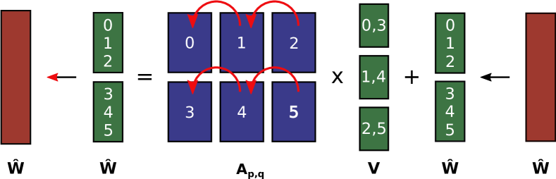
(a) $\hat{W}=A*\hat{V}+\hat{W}$.

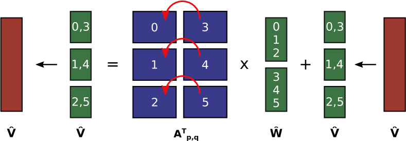
(b) $\hat{V}=A^{T}*\hat{W}+\hat{V}$.

Figure 1. An example of the Multi-GPU HEMM on 6 GPUs per MPI rank. Matrices/blocks stored in CPU (red) and GPU (green and blue) memory. The numbers denote the GPUs in which a block is stored.

3.3.2. Offloading Selected Routines to GPUs

In ChASE-CPU, all dense linear algebra operations other than HEMM have been implemented redundantly on each MPI process using threaded BLAS and LAPACK. For ChASE-GPU, the most computationally intensive operations have been offloaded to GPUs using NVIDIA shared-memory libraries cuBLAS and cuSOLVER. The API of cuBLAS and cuSOLVER is almost identical to that of BLAS and LAPACK, hence offloading them is a straightforward process.

Because the communication between CPUs and GPUs should be minimized and the device memory of a single GPU is limited, only the most compute-intensive operations have been offloaded to GPUs. First we offload the QR factorization using the cuSOLVER routine cusolverDnXgeqrf. Other selected operations are in the Rayleigh-Ritz procedure. In ChASE, the original eigenproblem is projected onto a "search" subspace, from which approximate solutions are computed. The active subspace is obtained by forming a ${\sf nev}\times{\sf nev}$ Rayleigh-Ritz quotient $G=\hat{Q}^{T}A\hat{Q}$, where $\hat{Q}$ is the $n\times{\sf nev}$ orthonormal matrix outputted by the QR factorization. In ChASE, the right-multiplication of $\hat{Q}$ with $A$ is implemented by utilizing the available distributed multi-GPUs HEMM. The left-multiplying $\hat{Q}^{T}$ on $A\hat{Q}$ is offloaded to GPUs using the cuBLAS cublasXgemm routine. Then $G$ is diagonalized as $G=\hat{W}\hat{\Lambda}\hat{W}^{-1}$ using a LAPACK eigensolver such as Divide&Conquer, with ($\hat{W},\hat{\Lambda}$) being the approximate eigenpairs of $G$. The diagonalization of $G$ is not performed on GPUs even if it would probably end up in a faster performance thanks to less data movement between CPU and GPU. This design choice is deliberate and is based on the trade-off between the large memory requirement of the diagonalization and its relative small speedup over vendor-optimized LAPACK. The eigenvectors of the original problem are obtained by a backtransform operation $\hat{Q}\hat{W}$, which is also offloaded to GPUs using the cublasXgemm routine.

Calling a cuBLAS or cuSOLVER routine requires allocating device memory for the input/output arrays and external workspace. This allocation is performed before the main work of ChASE by pre-computing the required buffer size, which is then reused whenever is possible, and deallocated only after the main work ends. This implementation avoids frequent allocation and deallocation of device memory in the loop between Line 5 and 17 (Algorithm 1), which is important to reduce the CPU-GPU synchronizations. The data movement between host and device memory is limited since it takes place only once for each iteration within the main loop of ChASE. In future work we plan to explore GPU-aware MPI for the direct communications between GPUs.

3.4. Estimating Memory Requirement

An important aspect of running ChASE is its memory footprint. The memory cost per task and per GPU device should not exceed the amount of main and device memory available. For this reason, we provide explicit formulas for estimating the memory cost of CPUs and GPUs in ChASE-GPU. The same formulas are encoded in a Python script (provided with the code) that the user can run to determine an appropriate resource allocation for a given problem.

The main memory requirement per MPI rank is given as follows

(6) $$M_{cpu}=pq+(p+q)n_{e}+2n_{e}n,$$

where $n$ is the rank of the matrix $A$ defining the eigenproblem, $n_{e}=\textsf{nev}+\textsf{nex}$ is the largest dimension of the active subspace to be projected onto. The dimension of the 2D MPI grid is defined as $r\times c$, and the dimension of the local matrix held by each MPI rank is $p\times q$, where $p=\frac{n}{r}$ and $q=\frac{n}{c}$. Because of their dependence on $r$ and $c$, the first two terms of Equation 6 scale with the increase in computational resources, while the last term does not, since it refers to a part of the code that is redundantly executed. The non-scalable part is negligible if $n_{e}$ is a small percentage of $n$.

A similar expression holds for the memory requirement per GPU

(7) $$M_{gpu}=\frac{pq}{r_{g}c_{g}}+3\max(\frac{p}{r_{g}},\frac{q}{c_{g}})n_{e}+(2n+n_{e})n_{e},$$

In ChASE-GPU, multiple GPUs of a single compute node can bind to an MPI process as a $r_{g}\times c_{g}$ 2D grid scheme. The first two terms of Equation 7 also scale with resource allocation. As for the CPU formula, the last term, which is $\mathcal{O}(n_{e}n)$, mainly refers to the memory requirements of cublasXgemm and cusolverDnXgeqrf, which are offloaded to GPUs and do not scale with the increase in MPI tasks. Since the capacity of device memory is limited compared to the main memory, this last term sets a maximum size for matrix $A$ and the number of eigenpairs that can be computed. In future work, we plan to remove these constraints by implementing versions of the related dense linear algebra operations distributed on a local subset of computing nodes.

When comparing ChASE memory footprint with the typical symmetric eigensolver in ScaLAPACK (e.g. PDSYEVX based on parallel bisection and inverse iteration), we notice a similar leading order behavior. PDSYEVX requires $\mathcal{O}(\frac{n^{2}}{rc}\equiv pq)$ memory per processor (i.e. MPI rank) (Antonelli and Vömel, 2005). However, depending on the spectrum (e.g. tightly clustered eigenvalues), the algorithm solving the tridiagonal form may require $\mathcal{O}(n^{2})$ memory per processor to guarantee the correctness of the computed eigenpairs. So we conclude that, while in the general the ChASE CPU memory requirement is slightly larger than ScaLAPACK solvers and has a non-scalable portion that depends on the global dimension of A ($n$), this portion is not leading order. Moreover, because this portion is related to the redundant QR factorization, future development in distributing such factorization will significantly decrease its impact to the overall ChASE memory footprint.

4. Numerical experiments

ChASE has been tested on JURECA-DC supercomputer at Jülich Supercomputing Centre. Each node is equipped with two 64 cores AMD EPYC 7742 CPUs @ 2.25 GHz ($16\times 32$ GB DDR4 Memory) and four NVIDIA Tesla A100 GPUs ($4\times 40$ GB high-bandwidth memory). ChASE is compiled with GCC 9.3.0, OpenMPI 4.1.0 (UCX 1.9.0), CUDA 11.0 and Intel MKL 2020.4.304. All computations in this section are performed in double-precision.

4.1. Test matrix suite

For benchmarking ChASE, we use artificial matrices whose eigenpairs are known analytically and random matrices generated with given spectral properties. The framework for the matrix generation is inspired by the testing infrastructure for symmetric tridiagonal eigensolvers of LAPACK (Marques et al., 2008). In this work, double precision artificial matrices are generated with four different spectral distributions.

The first two generated matrices have analytical eigenvalues and are named (1-2-1) and Wilkinson. (1-2-1) is a tridiagonal matrix with entries on the main diagonal and first two subdiagonals equal to $2$ and $1$, respectively. The Wilkinson matrix is another tridiagonal matrix whose entries on the first subdiagonals are all $1$, while the main diagonal have values $(m,m-1,m-2,\cdots,2,1,2,\cdots,m-2,m-1,m)$, in which $m=\frac{n-1}{2}$ with $n$ the size of matrix.

The next two generated matrices, Uniform and Geometric, are dense, symmetric with a given spectral distribution. In order to generate them we construct a diagonal matrix $D$ whose diagonal is filled exactly by the prescribed eigenvalues. Then a dense matrix $A$ with the given spectra is generated as $A=Q^{T}DQ$, with $Q$ an orthogonal matrix, and $Q^{T}$ its transpose. The orthogonal matrix $Q$ is the Q factor of a QR factorization on a $n\times n$ matrix whose entries are randomly generated with respect to the Gaussian distribution. All the matrices used in our tests are generated using our matrix generator which allow the creation of matrices of any desired size for both shared-memory and distributed-memory architectures.

Table 1. Spectral information for generating test matrices. In this table, we have $k=1,\cdots,n$.

Matrix Name	Spectral Distribution
Uniform (Uni)	$\lambda_{k}=d_{max}(\epsilon+\frac{(k-1)(1-\epsilon)}{n-1})$
Geometric (Geo)	$\lambda_{k}=d_{max}\epsilon^{\frac{n-k}{n-1}}$
(1-2-1) (1-2-1)	$\lambda_{k}=2-2\cos(\frac{\pi k}{n+1})$
Wilkinson (Wilk)	All positive, but one, roughly in pairs.

The spectral properties of four types of artificial matrices are given in Table 1 and are explained below:

• Uniform matrix: its eigenvalues are distributed equally within $[\min(d_{max}\epsilon,0),\max(d_{max}\epsilon,0)]$ following a discrete uniform distribution.

• Geometric matrix: its spectrum follows a geometric distribution. If $d_{max}>0$ and $\epsilon\in(0,1)$, then its eigenvalues are in the range $(0,d_{max}\epsilon]$, and smaller eigenvalues are quite more clustered than the larger ones.

• (1-2-1) matrix (Gregory, 1978; Higham, 1991) has analytically known eigenvalues. The clustering of its eigenvalues is not very strong, although clustering becomes tighter with the increase of dimension (Marques et al., 2008).

• For Wilkinson matrix, all eigenvalues, but one, are positive. The positive eigenvalues are roughly in pairs, and the larger pairs are closer together.

Because of their distinct spectral proprieties, these 4 types of matrices should provide a qualitative picture of the behavior of the ChASE library resulting in widely different numerical responses and performance measurements.

Table 2. Comparison of ChASE-CPU and ChASE-GPU with artificial matrices. The size of test matrices are $20\text{k}\times 20\text{k}$, and nev and nex are $1500$ and $500$, respectively. Statistics for each test are obtained over $20$ runs.

Matrix	Iter.	Matvecs	Runtime (seconds)
			All	Lanczos	Filter	QR	RR	Resid
1-2-1	13	466614	$272.28\pm 5.28$	$4.64\pm 0.19$	$176.46\pm 4.60$	$31.69\pm 1.27$	$37.45\pm 1.64$	$20.99\pm 0.67$
Geo	8	285192	$165.39\pm 1.86$	$4.76\pm 0.28$	$108.02\pm 1.75$	$19.19\pm 0.59$	$20.64\pm 1.22$	$12.14\pm 0.54$
Uni	5	163562	$101.27\pm 1.98$	$4.76\pm 0.24$	$62.17\pm 1.47$	$12.05\pm 0.53$	$13.91\pm 0.98$	$7.97\pm 0.60$
Wilk	9	248946	$155.44\pm 2.64$	$4.86\pm 0.96$	$95.68\pm 1.77$	$21.53\pm 0.88$	$20.62\pm 1.25$	$12.09\pm 0.47$

(a) ChASE-CPU on one node of JURECA-DC: MPI process number is $16$, and OpenMP thread number per rank is $8$.

Matrix	Iter.	Matvecs	Runtime (seconds)
			All	Lanczos	Filter	QR	RR	Resid
1-2-1	13	466614	$31.39\pm 0.09$	$0.58\pm 0.01$	$14.38\pm 0.02$	$2.59\pm 0.01$	$8.41\pm 0.09$	$5.24\pm 0.04$
Geo	8	285192	$18.57\pm 0.05$	$0.58\pm 0.01$	$8.76\pm 0.02$	$1.58\pm 0.01$	$4.58\pm 0.04$	$2.96\pm 0.02$
Uni	5	163562	$11.79\pm 0.03$	$0.58\pm 0.01$	$5.06\pm 0.00$	$1.00\pm 0.00$	$3.11\pm 0.04$	$1.96\pm 0.02$
Wilk	8	246924	$17.22\pm 0.05$	$0.57\pm 0.00$	$7.63\pm 0.02$	$1.59\pm 0.00$	$4.45\pm 0.04$	$2.90\pm 0.02$

(b) ChASE-GPU on one node of JURECA-DC: MPI process number is $4$, OpenMP thread and GPU number per process is $32$ and $1$.

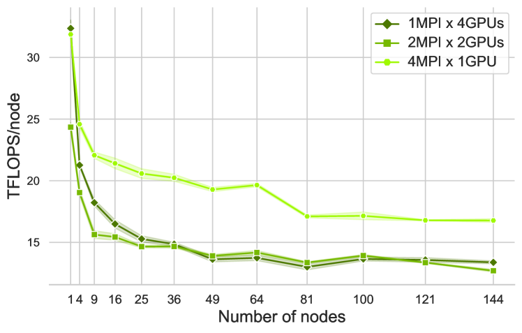
(a) Comparison of Filter’s performance in TFLOPS/node.

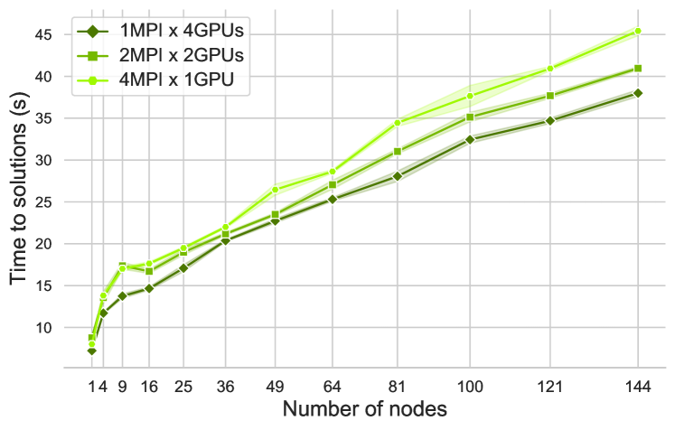
(b) Comparison of time-to-solution of ChASE.

Figure 2. Evaluation of three MPI and GPU binding configurations: 1, 2 and 4 MPI rank with 32 threads each and 4 GPUs in total. Data are obtained as the averages of 20 repetitions.

4.2. Evaluation of MPI and GPU Binding Configurations

As shown in Section 3.3, ChASE-GPU supports a flexible binding policy of MPI ranks and GPUs. In order to find the best configuration on the targeting platform JURECA-DC, we initially performed a weak scaling test with three binding policies of MPI ranks and GPUs within node: (1) 1 MPI rank bounded with 4 GPUs ($1$MPI$\times 4$GPUs), (2) 2 MPI ranks with 2 GPUs bounded to each ($2$MPI$\times 2$GPUs), (3) 4 MPI ranks with 1 GPU bounded to each ($4$MPI$\times 1$GPUs). The number of threads per rank is fixed to $32$ so as to eliminate the huge NUMA-effects of some BLAS and LAPACK routines.

For the weak scaling experiment, the numbers of compute nodes are $p^{2}$, with $p\in 1,2,\cdots,12$ to produce 2D square node grids. The generated test matrices are of type Uniform with sizes being $3\times 10^{4}p$. The number of desired eigenpairs nev and external searching space increment nex are $2250$ and $750$, respectively.

In this section, for all three configurations, we report both the performance of the Filter and the time-to-solution of ChASE-GPU. The Filter, whose major part is the HEMM, is reported as the absolute performance extracted from the GPUs with tensor core activated. Because the FP64 Tensor Core is used automatically and selectively by cuBLAS 11.0.0 we report absolute performance and not fraction of peak. The performance of the Filter directly reflects the performance of the multi-GPU HEMM, which is one of the original contributions of this paper. In the case of weak scaling, both the number of computing units and the problem size increase, which results in a constant workload per units. However, for an iterative eigensolver, it is impossible to predict exactly the total workload to reach convergence, even if the problems are constructed with matrices sharing the same spectral distribution. Instead of solving problems to achieve full convergence, each test of weak scaling has been executed with only one subspace iteration, which can ensure a constant workload of Matvecs per computing unit.

Fig. 2a shows that the performance of the Filter decreases rapidly for all three configurations as the number of compute nodes increases, stabilising when the number of compute nodes is greater than 16. The reason for the performance drop is that communication (collective routine MPI_Allreduce) and memory copies between CPU and GPU are included in the total execution time of the Filter. In (Zhang et al., 2021) (see Supplementary Materials, Table S7), the authors showed that the latency in MPI_Allreduce remains constant on more than 16 nodes, as does the impact of MPI communication on Filter performance. This is clearly observed in the 1MPIx4GPU configuration when the number of nodes is increased from 1 to 4, as no MPI communication was required on one node (only 1 MPI rank is used). At each step in the Filter, a rectangular block of vectors $V$ is split (see Eq. 2) and distributed to the GPUs of the same node and copied back to the host memory after the matrix multiplication is completed. These two operations (and $N=120k$) consume $~{}30\%$ of the total time of the distributed HEMM. In addition, some extra time ($~{}19\%$) is spent on inter-GPU communication at the node level, so up to $50\%$ of the HEMM time is spent on the memory copy. The memory copies cannot be efficiently overlapped with matrix-matrix multiplication because there is a strong dependency between them. Currently, this multi-GPU HEMM lacks support for faster communication links between GPUs within the node, such as. NVLink, and is part of future work.

Fig. 2b shows that the time-to-solution for ChASE with all three configurations increases somewhat linearly as a function of the number of compute nodes used. The performance of the entire ChASE is different from the performance of the Filter in Fig. 2a. ChASE with configuration $1$MPI$\times 4$GPUs always outperforms the other two, with $2$MPI$\times 2$GPUs in between. Since QR and RR are computed redundantly on each MPI rank and operate on the full column size, the gain of the configuration with $1$MPI$\times 4$GPUs over the other configurations comes from a lower communication overhead using expensive MPI_Ibcast (see (Zhang et al., 2021), Supplement Materials, Table S7). Unlike MPI_Allreduce, the latency of the broadcasting routines increases steadily with the number of MPI ranks.

The outcome of its higher efficiency due to the decreased MPI communication makes up the relative lower performance of its corresponding Filter. Because $1$MPI$\times 4$GPUs is the best configuration of ChASE-GPU on JURECA-DC, we will use it as the default configuration for the remaining tests. Additional weak scaling tests are discussed in Section 4.4.2.

4.3. Eigen-type tests

In order to confirm the numerical robustness of ChASE-GPU, we compare it with ChASE-CPU using the test matrix suite described in Section 4.1. The size of the test matrices is fixed as $20$k, and nev and nex are respectively $1500$ and $500$, which means the maximum size of active subspace is $10$% of the full space of problems. The $\ell^{2}$-norm condition numbers of generated (1-2-1), Geometric, Uniform and Wilkinson matrices are respectively $1.6\times 10^{8}$, $1.0\times 10^{4}$, $1.0\times 10^{4}$ and $4.7\times 10^{4}$.

The experiments of both ChASE-CPU and ChASE-GPU are performed on one single compute node with a different combination of MPI ranks and OpenMP threads for each of the two versions of ChASE. For ChASE-CPU, the number of MPI ranks and OpenMP threads per node is fixed at $16$ and $8$, respectively. This is the best combination of MPI and OpenMP on JURECA-DC, and was obtained from a series of sweet-spot tests spanning all possible combinations. For ChASE-GPU, the configuration is $1$MPI$\times 4$GPUs, and the number of OpenMP threads per MPI rank is $32$, which has been proved as the best one.

The results are shown in Table 2, which includes the subspace iteration number until convergence, the required number of Matvecs operations, and the runtime for ChASE and its main parts. For all four types of eigenproblems, both ChASE-CPU and ChASE-GPU are able to achieve the convergence in a limited number of iterations with the (1-2-1) problem, which has a much larger condition number, taking the most time and iterations, more than doubling the runtime and iterations of the Uniform problem. The acceleration provided by ChASE-GPU is practically independent from the type of eigenproblem. For all four test matrices, ChASE-GPU achieves a speedup of approximately $8.9\times$ for the entire runtime and $12.7\times$ for just the Filter, which is the most computationally intensive part of the solver. The considerations above demonstrate the viability of ChASE as a general purpose solver for extremal symmetric eigenproblems. Because they converge faster than the others, we will generate only eigenproblems of the Uniform type for the scalability tests.

A closer look reveals that the exact number of iterations between ChASE-CPU and ChASE-GPU differs for the matrix Wilkinson. This difference is also reflected in the numbers of Matvecs. This may seem an harmless difference, but it is rather suspicious in light of the deterministic convergence provided by the Chebyshev filter (Winkelmann et al., 2019). Upon further investigation, we identified the cause of this behavior in a very peculiar numerical instability of cusolverXgeqrf, the QR factorization of cuSOLVER, which seems to happen randomly. The numerical difference of QR factorization between the one in cuSOLVER and LAPACK is minor, just above the machine precision. However, this difference propagates through the computation, which finally results in a slightly different numerical accuracy. We further observed that for much larger matrices than $20$k such numerical instability can sometimes damage the redundant computations of the QR factorization and introduce a mismatch in the data exchanged between different rows of MPI communicators. Eventually this behavior results in the breakdown of ChASE-GPU. We have signalled the bug to the NVIDIA developers of cuSOLVER.

4.4. Scalability

This section analyze ChASE-GPU’s behavior in strong and weak scalability regime by comparing with ChASE-CPU. For all the tests, the numbers of MPI ranks and OpenMP threads per rank of ChASE-CPU are respectively $16$ and $8$. For ChASE-GPU, the number of MPI ranks per node is $1$, with $4$ GPUs and $32$ threads assigned to each rank.

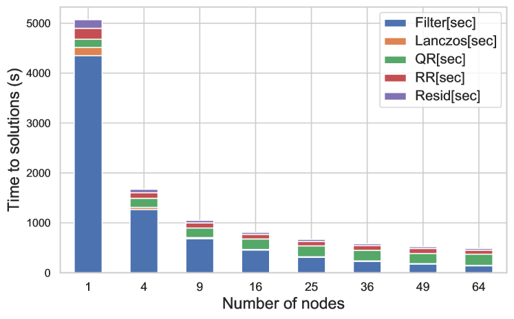
(a) Strong scaling performance of ChASE-CPU.

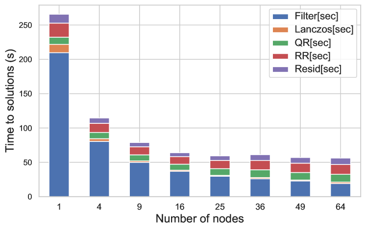
(b) Strong scaling performance of ChASE-GPU.

Figure 3. Strong scaling tests with Uniform matrix ($n=130,000$, nev$=1000$, and nex$=300$). Data are obtained as the averages of 15 repetitions.

4.4.1. Strong scaling

Fig. 3 illustrates the results of the strong scaling experiment of ChASE-CPU and GPU using a Uniform matrix of size $n=130,000$. We fix nev and nex respectively as $1000$ and $300$ ($=1$%n). The counts of compute nodes are selected to be square numbers $1,4,9,\cdots,64$. Fig. 3 reports the runtime of ChASE-CPU and ChASE-GPU as a vertical stacked bar plot, which includes also the fractions of runtime of numerical functions, such as Filter, Lanczos, QR, RR and Resid. The speedup of ChASE-GPU is plotted in Fig. 4, where for each point on the x-axis, the speedup is calculated with respect to the corresponding timing of ChASE-CPU.

Both ChASE-CPU and ChASE-GPU can achieve good strong scaling performance for smaller number of nodes. However, with larger number of compute nodes, the decrease of total runtime of ChASE become progressively negligible, especially for ChASE-GPU. The Filter, whose most important operation is the customized HEMM, achieves very good strong scaling performance in both ChASE-CPU and ChASE-GPU. Compared with the tests using $1$ compute node, ChASE-CPU with $64$ compute nodes achieves $32\times$ speedup for Filter, $29\times$ speedup for Lanczos, and $5\times$ speedup for Resid. Analogously, ChASE-GPU achieves $10.8\times$ speedup for Filter, $5\times$ speedup for Lanczos, but only $1.4\times$ speedup for Resid. For ChASE-CPU, the most dominant linear algebra operation in the Filter, Lanczos and Resid is HEMM. In these three functions in ChASE-GPU, only HEMM has been offloaded to GPUs, which achieves a notable acceleration over the CPU version. Compared to HEMM, the remaining BLAS/LAPACK operations called within the Lanczos and Resid become much more dominant, which turn them into new bottlenecks. This is also the reason why the strong scaling performance of ChASE-GPU tends to be worse than ChASE-CPU, even with the acceleration of GPUs. This is clearly visible from Fig. 4, which shows the speedup of ChASE-GPU over ChASE-CPU as a function of compute nodes count. ChASE-GPU with $1$ compute node has the maximal speedup over ChASE-CPU, which is $19.16$. Increasing the count of compute node, the speedup keeps getting smaller and tends to flatten towards a value $\sim 8.61$.

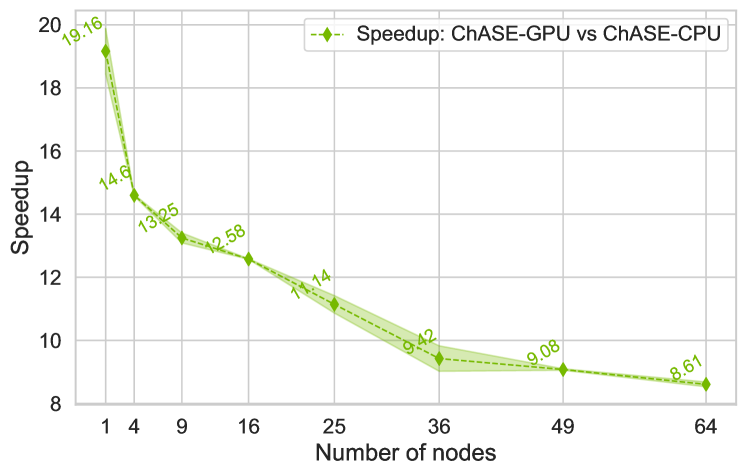
Figure 4. Strong scaling: Speedup. Speedup of ChASE-GPU over ChASE-CPU. Error bars are obtained with 15 repetitions.

4.4.2. Weak scaling

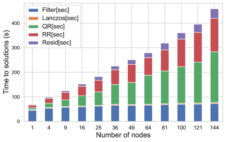
(a) Weak scaling performance of ChASE-CPU.

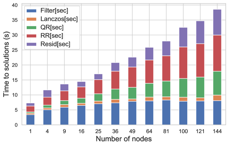
(b) Weak scaling performance of ChASE-GPU.

Figure 5. Weak scaling tests with Uniform matrix ($n$ ranging from $30$k to $360$k, nev$=2250$, nex$=750$). Data are obtained as the averages of 15 repetitions.

Weak scaling experiments are particularly important to domain scientists, who are interested in simulating system of increasingly larger size. In order to maintain a fixed workload, we keep the same setup described in Section 4.2. The test matrices are of type Uniform, with size increment of $30$k ($30\text{k},60\text{k},90\text{k},\cdots,360\text{k}$). The counts of compute nodes selected as square numbers $1,4,9,\cdots,144$, and nev and nex are respectively fixed as $2250$ and $750$. Fig. 5 plots the results of weak scaling experiments as a vertical stacked bar plot, which shows the runtime of ChASE-CPU and ChASE-GPU, including the runtime of their numerical functions. Additionally, Fig. 6 reports the parallel efficiency of the numerical functions Filter and Resid of this weak scaling experiment.

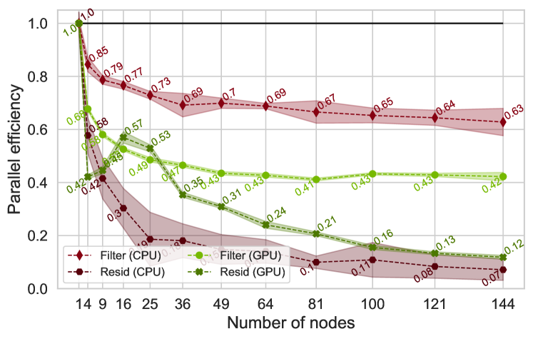
Figure 6. Weak scaling: Parallel efficiency of Filter and Resid. Error bars are obtained with 15 repetitions.

The good news is that, independently of which version, ChASE scale linearly. The bad news is that the total runtime of ChASE-CPU and ChASE-GPU doubles every-time the matrix size quadruples and triples, respectively. When we look at the details of the distribution of runtime over the different functions, we observe a good weak scaling of the Filter thanks to the custom parallelization of HEMM for both CPU and GPU. However, a small increase in Filter runtime is observed when the number of nodes is increased, e.g. to 1, 4 and 16 nodes (Fig. 5b) the runtime is  3.27 sec,  5.01 sec and  6.3 sec, respectively. The main reason for this is an increased amount of communication (MPI_Allreduce). The percentage of MPI on 4 and 16 nodes is 35% and 49% of the total Filter execution time, respectively. However, considering only the distributed HEMM performance (without MPI communication) on 16 nodes with 64 GPUs, we reach 685.44 TFlops ( 55% of the peak GPU performance). The increased communication is expected because Allreduce is called at the end of the distributed HEMM which is computed multiple times within the Filter and could be repeated up to $20$ times (the maximum degree of the polynomial) in the first iteration of ChASE.

The weak scaling of Lanczos and Resid are quite worse than the Filter, even if they make use of the distributed HEMM. With the increase of problem size, QR and RR, which are computed redundantly on the node, become progressively dominant, especially the QR factorization. For ChASE-CPU with $144$ compute nodes, QR and RR take $48$% and $29$% of the whole runtime, meanwhile Filter take only $16$%. In ChASE-GPU, the QR factorization and the GEMM routine, called internally by RR, have been offloaded to a single GPU using the cuSOLVER and the cuBLAS libraries. Such a choice makes these two functions less impactful than the corresponding one in ChASE-CPU.

Fig. 6 shows the parallel efficiency of Filter and Resid of both ChASE-CPU and ChASE-GPU. For $144$ compute nodes, the Filter in ChASE-CPU and ChASE-GPU shows a parallel efficiency of $63$% and $42\%$, respectively. On the other hand, the parallel efficiency of Resid in ChASE-CPU and ChASE-GPU attains $7$% and $12$%, respectively. Overall, our results confirms the efficiency of our implementation of distributed multi-GPU HEMM and provide a strong indication of what should be the focus of further developments of the ChASE library.

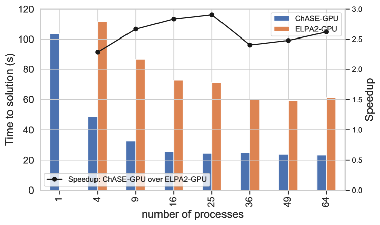
Figure 7. Strong scaling: Time-to-solution and speedup of ChASE-GPU over ELPA2 for solving 76k In₂O₃ Hermitian eigenproblem with nev=800. Data are obtained as the averages of 15 repetitions.

4.5. Comparison with other libraries

As we stated in Section 2, there are no other distributed GPU eigensolvers apart from ELPA2. Therefore, we perform a strong scaling test up to 64 compute nodes comparing ChASE-GPU with ELPA2 with GPU support (ELPA2-GPU). The comparison of ChASE-CPU with other libraries are not carried out in this paper, since the comparison with ScaLAPACK, Elemental and FEAST are available in (Winkelmann et al., 2019). The version of ELPA for the benchmarks is 2020.11.001, which is the most updated installation on JURECA-DC. The selected installation is compiled with GCC 10.3.0, OpenMPI 4.1.1, Intel MKL 2021.2.0 and CUDA 11.3 with CUDA architecture $sm\_80$. We prefer to use ELPA compiled with OpenMPI rather than the one compiled with ParaStationMPI, since the former enable ELPA to be 10% faster than the latter. The Multi-Process Service (MPS) is activated for ELPA. The MPI core and GPU numbers per node is set respectively as $32$ and $4$. This configuration has been selected based on a sweet-spot test with multiple configurations. The 2D grid of MPI ranks is setup as closest to be square. The block size of the block-cyclic distribution of matrix in ELPA is fixed at $16$.

The eigenproblem that we use for this test is Hermitian with a matrix size 76k, and is generated by the discretization of the Bethe-Salpeter equation used to simulate the opto-electornic properties of In₂O₃. The number of eigenpairs sought after, nev, is set at $800$ for both ChASE-GPU and ELPA2-GPU. For ChASE-GPU, the size of the external searching space nex is fixed as $200$. The time-to-solution and speedup of ChASE-GPU over ELPA2-GPU is reported in Fig. 7.

We first point out that ELPA2-GPU runs out of device memory when only 1 compute node is used, while ChASE-GPU solves successfully the problem in $104$ seconds. The strong scaling performance of ChASE-GPU is also better than the one of ELPA2-GPU, especially with a relative small number of compute nodes. For instance, ChASE-GPU shows a $1.88\times$ speedup when the compute node number increases from $4$ to $16$, meanwhile ELPA2-GPU displays only $1.54\times$ speedup. In average, ChASE-GPU achieves $2.6\times$ speedup over ELPA2 when the compute node number ranges from $4$ to $16$. The maximal speedup $2.97\times$ has been achieved when $25$ compute nodes are used.

We point out that the performance gain of ChASE-GPU over ELPA2-GPU has been obtained when only a relatively small portion of extremal eigenpairs are sought after, which is the range of viability of the ChASE library. In this case, ChASE-GPU can achieve large speedup over ELPA2-GPU with an inferior memory footprint.

5. Conclusion

In this paper, we presented a distributed CPU-GPU implementation of the ChASE eigensolver for large-scale symmetric eigenproblems. ChASE targets extremal dense eigenproblems when a relatively small fraction ($\leq 10$%) of extremal eigenpairs is sought after. We introduce the implementation of a customized distributed CPU-GPU HEMM for ChASE which is used in many of its functions, notably the Chebyshev filter. Because the Filter function is the most computationally heavy part of the library, this custom-HEMM implementation has a dramatic impact on the parallel performance of the library when is ported on distributed multi-GPUs architectures. We have benchmarked the numerical and parallel performance of the new distributed hybrid CPU-GPU implementation on one of the most modern platforms featuring AMD Epyc Rome CPUs coupled with 4 powerful NVIDIA A100. Our tests show a good parallel performance of the custom HEMM implementation impacting positively the overall performance of the library. Because of the excellent scaling of the Filter using the new HEMM, other functions in the library have become the new bottleneck which we plan to addressed in the near future. The overall target, is to further develop ChASE into an eigensolver that can be deployed and used on current PETAscale supercomputing clusters to solve for very large eigenproblems.

6. Acknowledgments

This work was supported by the Croatian Science Foundation under grant number HRZZ-UIP-2020-02-4559, by the Ministry of Science and Education of the Republic of Croatia and the Deutsche Akademische Austauschdienst (DAAD) from fund of the Bundesministeriums für Bildung und Forschung (BMBF) through project "PPP Kroatien" ID 57449075. This work was also partially supported by PRACE-6IP WP8: Performance Portable Linear Algebra (grant agreement ID 823767).

References

- (1)
- Anderson et al. (1999) Edward C Anderson, Zhaojun Bai, Christian H. Bischof, L S Blackford, James W. Demmel, Jack Dongarra, Jeremy J Du Croz, Anne Greenbaum, A. Hammarling, S. McKenney, and Danny C Sorensen. 1999. {LAPACK} Users’ Guide. Society for Industrial and Applied Mathematics, Philadelphia, PA.
- Antonelli and Vömel (2005) Dominic Antonelli and Christof Vömel. 2005. PDSYEVR. ScaLAPACK’s Parallel MRRR Algorithm for the Symmetric Eigenvalue Problem. LAPACK Working Note 168 (2005), 1–18. http://www.netlib.org/lapack/lawnspdf/lawn168.pdf
- Ashby (1991) Steven F Ashby. 1991. Minimax Polynomial Preconditioning for Hermitian Linear Systems. SIAM J. Matrix Anal. Appl. 12, 4 (1991), 766–789.
- Banerjee et al. (2016) Amartya S. Banerjee, Lin Lin, Wei Hu, Chao Yang, and John E. Pask. 2016. Chebyshev Polynomial Filtered Subspace Iteration in the Discontinuous Galerkin Method for Large-Scale Electronic Structure Calculations. The Journal of Chemical Physics 145, 15 (Oct. 2016), 154101. https://doi.org/10.1063/1.4964861
- Bauer (1957) Friedrich L. Bauer. 1957. Das Verfahren der Treppeniteration und verwandte Verfahren zur Lösung algebraischer Eigenwertprobleme. Zeitschrift für Angewandte Mathematik und Physik ZAMP 8, 3 (May 1957), 214–235. https://doi.org/10.1007/BF01600502
- Becke (1993) Axel D Becke. 1993. A new Mixing of Hartree-Fock and Local Density-functional Theories. The Journal of chemical physics 98, 2 (1993), 1372–1377.
- Berljafa et al. (2015) Mario Berljafa, Daniel Wortmann, and Edoardo Di Napoli. 2015. An Optimized and Scalable Eigensolver for Sequences of Eigenvalue Problems. Concurrency and Computation: Practice and Experience 27 (Sept. 2015), 905–922. https://doi.org/10.1002/cpe.3394
- Bientinesi et al. (2005) Paolo Bientinesi, Inderjit S Dhillon, and Robert A Van De Geijn. 2005. A Parallel Eigensolver for Dense Symmetric Matrices based on Multiple Relatively Robust Representations. SIAM Journal on Scientific Computing 27, 1 (2005), 43–66.
- Choi et al. (2003) J. Choi, J.J. Dongarra, R. Pozo, and D.W. Walker. 2003. ScaLAPACK: a Scalable Linear Algebra Library for Distributed Memory Concurrent Computers. In [Proceedings 1992] The Fourth Symposium on the Frontiers of Massively Parallel Computation. IEEE Comput. Soc. Press, Los Alamitos, CA, USA, 120–127. https://doi.org/10.1109/FMPC.1992.234898
- Dhillon et al. (2006) Inderjit S Dhillon, Beresford N Parlett, and Christof Vömel. 2006. The Design and Implementation of the MRRR Algorithm. ACM Transactions on Mathematical Software (TOMS) 32, 4 (2006), 533–560.
- ELPA (2014) ELPA. 2014. Eigenvalue Solvers for Petaflop-Applications (ELPA). https://elpa.mpcdf.mpg.de/
- Fukaya and Imamura (2015) Takeshi Fukaya and Toshiyuki Imamura. 2015. Performance Evaluation of the Eigen Exa eigensolver on Oakleaf-FX: Tridiagonalization versus pentadiagonalization. In 2015 IEEE International Parallel and Distributed Processing Symposium Workshop. IEEE, 960–969.
- Fukaya et al. (2018) Takeshi Fukaya, Toshiyuki Imamura, and Yusaku Yamamoto. 2018. A Case Study on Modeling the Performance of Dense Matrix Computation: Tridiagonalization in the Eigenexa Eigensolver on the K Computer. In Proceedings - 2018 IEEE 32nd International Parallel and Distributed Processing Symposium Workshops, IPDPSW 2018. Institute of Electrical and Electronics Engineers Inc., 1113–1122. https://doi.org/10.1109/IPDPSW.2018.00171
- Gates et al. (2019) Mark Gates, Jakub Kurzak, Ali Charara, Asim Yarkhan, and Jack Dongarra. 2019. SLATE: Design of a Modern Distributed and Accelerated Linear Algebra Library. In International Conference for High Performance Computing, Networking, Storage and Analysis, SC. IEEE Computer Society, New York, NY, USA, 1–18. https://doi.org/10.1145/3295500.3356223
- Gregory (1978) Robert T Gregory. 1978. A Collection of Matrices for Testing Computational Algorithms. Technical Report.
- Haidar et al. (2014) Azzam Haidar, Stanimire Tomov, Jack Dongarra, Raffaele Solcà, and Thomas Schulthess. 2014. A Novel Hybrid CPU–GPU Generalized Eigensolver for Electronic Structure Calculations based on Fine-grained Memory Aware Tasks. The International Journal of High Performance Computing Applications 28, 2 (2014), 196–209. https://doi.org/10.1177/1094342013502097 arXiv:https://doi.org/10.1177/1094342013502097
- Higham (1991) Nicholas J Higham. 1991. Algorithm 694: A Collection of Test Matrices in MATLAB. ACM Transactions on Mathematical Software (TOMS) 17, 3 (1991), 289–305.
- Ikegami et al. (2010) Tsutomu Ikegami, Tetsuya Sakurai, and Umpei Nagashima. 2010. A Filter Diagonalization for Generalized Eigenvalue Problems based on the Sakurai–Sugiura Projection Method. J. Comput. Appl. Math. 233, 8 (2010), 1927–1936.
- Imamura et al. (2011) Toshiyuki Imamura, Susumu Yamada, and Masahiko Machida. 2011. Development of a High Performance Eigensolver on the Petascale next Generation Supercomputer System. Progress in Nuclear Science and Technology 2 (2011), 643–650.
- Kestyn et al. (2016) James Kestyn, Vasileios Kalantzis, Eric Polizzi, and Yousef Saad. 2016. PFEAST: a High Performance Sparse Eigenvalue Solver using Distributed-memory Linear Solvers. In SC’16: Proceedings of the International Conference for High Performance Computing, Networking, Storage and Analysis. IEEE, 178–189.
- Kohn (1999) Walter Kohn. 1999. Nobel Lecture: Electronic Structure of Matter—wave Functions and Density Functionals. Reviews of Modern Physics 71, 5 (1999), 1253.
- Kohn and Sham (1965) Walter Kohn and Lu Jeu Sham. 1965. Self-consistent Equations including Exchange and Correlation Effects. Physical review 140, 4A (1965), A1133.
- Levitt and Torrent (2015) Antoine Levitt and Marc Torrent. 2015. Parallel Eigensolvers in Plane-Wave Density Functional Theory. Computer Physics Communications 187 (Feb. 2015), 98–105. https://doi.org/10.1016/j.cpc.2014.10.015
- Lin et al. (2016) Lin Lin, Yousef Saad, and Chao Yang. 2016. Approximating Spectral Densities of Large Matrices. SIAM Rev. 58, 1 (2016), 34–65. https://doi.org/10.1137/130934283
- Marek et al. (2014) Andreas Marek, Volker Blum, Rainer Johanni, Ville Havu, Bruno Lang, Thomas Auckenthaler, Alexander Heinecke, H-J Bungartz, and Hermann Lederer. 2014. The ELPA library: Scalable Parallel Eigenvalue Solutions for Electronic Structure Theory and Computational Science. Journal of Physics: Condensed Matter 26, 21 (5 2014), 213201. https://doi.org/10.1088/0953-8984/26/21/213201
- Marques et al. (2008) Osni A Marques, Christof Vömel, James W Demmel, and Beresford N Parlett. 2008. Algorithm 880: A Testing Infrastructure for Symmetric Tridiagonal Eigensolvers. ACM Transactions on Mathematical Software (TOMS) 35, 1 (2008), 1–13.
- Myllykoski and Kjelgaard Mikkelsen (2021) Mirko Myllykoski and Carl Christian Kjelgaard Mikkelsen. 2021. Task-based, GPU-accelerated and Robust Library for Solving Dense Nonsymmetric Eigenvalue Problems. Concurrency and Computation: Practice and Experience 33, 11 (2021), e5915. https://doi.org/10.1002/cpe.5915 arXiv:https://onlinelibrary.wiley.com/doi/pdf/10.1002/cpe.5915
- NVIDIA (2019) NVIDIA. 2019. cuSOLVER :: CUDA Toolkit Documentation. https://docs.nvidia.com/cuda/cusolver/
- NVIDIA (2021) NVIDIA. 2021. https://www.nvidia.com/en-us/data-center/grace-cpu. Accessed: 2021-10-06.
- Polizzi (2009) Eric Polizzi. 2009. Density-matrix-based Algorithm for Solving Eigenvalue Problems. Physical Review B 79, 11 (2009), 115112.
- Poulson et al. (2013) Jack Poulson, Bryan Marker, Robert A. Van De Geijn, Jeff R. Hammond, and Nichols A. Romero. 2013. Elemental: A New Framework for Distributed Memory Dense Matrix Computations. ACM Trans. Math. Software 39, 2 (2 2013), 1–24. https://doi.org/10.1145/2427023.2427030
- Rutishauser (1970) Heinz Rutishauser. 1970. Simultaneous Iteration Method for Symmetric Matrices. Numer. Math. 16, 3 (1970), 205–223. https://doi.org/10.1007/bf02219773
- Sakurai and Sugiura (2003) Tetsuya Sakurai and Hiroshi Sugiura. 2003. A Projection Method for Generalized Eigenvalue Problems using Numerical Integration. Journal of computational and applied mathematics 159, 1 (2003), 119–128.
- Sameh and Kuck (1977) Ahmed H Sameh and David J Kuck. 1977. A Parallel QR Algorithm for Symmetric Tridiagonal Matrices. IEEE Trans. Comput. 100, 2 (1977), 147–153.
- Thornquist (2006) Heidi K Thornquist. 2006. Fixed-polynomial Approximate Spectral Transformations for Preconditioning the Eigenvalue Problem. Rice University.
- Tisseur and Dongarra (1999) Françoise Tisseur and Jack Dongarra. 1999. A Parallel Divide and Conquer Algorithm for the Symmetric Eigenvalue Problem on Distributed Memory Architectures. SIAM Journal on Scientific Computing 20, 6 (1999), 2223–2236.
- Tomov et al. (2010) Stanimire Tomov, Jack Dongarra, and Marc Baboulin. 2010. Towards Dense Linear Algebra for Hybrid GPU Accelerated Manycore Systems. Parallel Comput. 36, 5-6 (jun 2010), 232–240. https://doi.org/10.1016/j.parco.2009.12.005
- Van Zee et al. (2009) Field G Van Zee, Ernie Chan, Robert A Van de Geijn, Enrique S Quintana-Orti, and Gregorio Quintana-Orti. 2009. The libflame Library for Dense Matrix Computations. Computing in science & engineering 11, 6 (2009), 56–63.
- Van Zee and Van De Geijn (2015) Field G Van Zee and Robert A Van De Geijn. 2015. BLIS: A Framework for Rapidly Instantiating BLAS Functionality. ACM Transactions on Mathematical Software (TOMS) 41, 3 (2015), 1–33.
- Wang et al. (2014) Endong Wang, Qing Zhang, Bo Shen, Guangyong Zhang, Xiaowei Lu, Qing Wu, and Yajuan Wang. 2014. Intel Math Kernel Library. In High-Performance Computing on the Intel® Xeon Phi™. Springer, 167–188.
- Williams-Young and Yang (2020) David B. Williams-Young and Chao Yang. 2020. Parallel Shift-Invert Spectrum Slicing on Distributed Architectures with GPU Accelerators. In 49th International Conference on Parallel Processing - ICPP. ACM, New York, NY, USA, 1–11. https://doi.org/10.1145/3404397.3404416
- Winkelmann et al. (2019) Jan Winkelmann, Paul Springer, and Edoardo Di Napoli. 2019. ChASE: Chebyshev Accelerated Subspace Iteration Eigensolver for Sequences of Hermitian Eigenvalue Problems. ACM Trans. Math. Software 45, 2 (jun 2019), 1–34. https://doi.org/10.1145/3313828
- Xianyi et al. (2012) Zhang Xianyi, Wang Qian, and Zaheer Chothia. 2012. OpenBLAS. URL: http://xianyi. github. io/OpenBLAS 88 (2012).
- Yu et al. (2021) Victor Wen zhe Yu, Jonathan Moussa, Pavel Kůs, Andreas Marek, Peter Messmer, Mina Yoon, Hermann Lederer, and Volker Blum. 2021. GPU-acceleration of the ELPA2 Distributed Eigensolver for Dense Symmetric and Hermitian Eigenproblems. Computer Physics Communications 262 (5 2021), 107808. https://doi.org/10.1016/j.cpc.2020.107808
- Zhang et al. (2021) Xiao Zhang, Sebastian Achilles, Jan Winkelmann, Roland Haas, André Schleife, and Edoardo Di Napoli. 2021. Solving the Bethe-Salpeter Equation on Massively Parallel Architectures. Computer Physics Communications 267 (2021), 108081. https://doi.org/10.1016/j.cpc.2021.108081
- Zhou et al. (2014) Yunkai Zhou, James R. Chelikowsky, and Yousef Saad. 2014. Chebyshev-Filtered Subspace Iteration Method Free of Sparse Diagonalization for Solving the Kohn-Sham Equation. J. Comput. Phys. 274 (Oct. 2014), 770–782.
- Zhou et al. (2006) Yunkai Zhou, Yousef Saad, Murilo L Tiago, and James R Chelikowsky. 2006. Parallel Self-Consistent-Field Calculations via Chebyshev-Filtered Subspace Acceleration. Physical Review E 74, 6 (2006), 066704. https://doi.org/10.1103/PhysRevE.74.066704