Testing the Ampère-Maxwell law on the photon mass and Lorentz-Poincaré symmetry violation with MMS multi-spacecraft data

Abstract

We investigate possible evidence from Extended Theories of Electro-Magnetism by looking for deviations from the Ampère-Maxwell law. The photon, main messenger for interpreting the universe, is the only free massless particle in the Standard-Model (SM). Indeed, the deviations may be due to a photon mass for the de Broglie-Proca (dBP) theory or the Lorentz-Poincaré Symmetry Violation (LSV) in the SM Extension (SME), but also to non-linearities from theories as of Born-Infeld, Heisenberg-Euler. With this aim, we have analysed six years of data of the Magnetospheric Multi-Scale mission, which is a four-satellite constellation, crossing mostly turbulent regions of magnetic reconnection and collecting about 95% of the downloaded data, outside the solar wind. We examined 3.8 million data points from the solar wind, magnetosheath, and magnetosphere regions. In a minority of cases, for the highest time resolution burst data and optimal tetrahedron configurations drawn by the four spacecraft, deviations have been found ($2.2\%$ in modulus and $4.8\%$ in Cartesian components for all regions, but raising up in the solar wind alone to $20.8\%$ in modulus and $29.7\%$ in Cartesian components and up to 45.2% in the extreme low-mass range). The deviations might be due to unaccounted experimental errors or, less likely, to non-Maxwellian contributions, for which we have inferred the related parameters for the dBP and SME cases. Possibly, we are at the boundaries of measurability for non-dedicated missions. We discuss our experimental results (upper limit of photon mass of $2.1\times 10^{-51}$ kg, and of the LSV parameter $|\vec{k}^{\rm AF}|$ of $6\times 10^{-9}$ m^-1), as the deviations in the solar wind, versus more stringent but model-dependent limits.

I Beyond Maxwellian theory: implications

Astrophysical observations are mostly based on electro-magnetic signals, interpreted with the standard Maxwellian massless and linear framework. Even when considering its overwhelming successes, the XIX century Maxwellian theory might be an approximation of a more comprehensive theory, as Newtonian gravity is for General Relativity. The linear description of the electro-magnetic phenomena by Maxwell’s theory and the unique photon masslessness, among all particles in the Standard-Model (SM) are questioned by the Extended Theories of Electro-Magnetism (ETEM). Herein, we test the Ampère-Maxwell (AM) law, by analysing millions of measured currents in the Earth neighbourhood.

The search for a deviation from the AM law complements other searches of manifestations or implications of ETEM physics among which

• vacuum birefringence: the refractive index is dependent on the polarisation and propagation direction Kostelecký and Mewes (2009); Li et al. (2015);

• frequency shifts associated with magnetars from non-linear quantum electro-dynamics Mosquera Cuesta and Salim (2004); Bonetti et al. (2017a);

• light dispersion: the group velocity differs from $c$ by a factor proportional to the inverse square of the frequency Bonetti et al. (2016); Bonetti et al. (2017b) with a bearing on i) multi-messenger astronomy Veske et al. (2021), ii)on pulsar timing Donner et al. (2019) and on gravitational wave detection at low frequencies via pulsars Antoniadis et al. (2023), due to plasma dispersion Bentum et al. (2017), iii) and on the estimates of the graviton mass Piórkowska-Kurpas (2022);

• frequency shift in vacuo in addition to the cosmological redshift due to the expansion of the Universe J. A. Helayël-Neto and Spallicci (2019); Spallicci et al. (2021); Spallicci et al. (2022a); Sarracino et al. (2022); thanks to this addition, a concordance between the luminosity and the redshift distances of Supernovae IA has been achieved, without requiring an accelerated expansion due to dark energy; for a complementary approach, see López-Corredoira and Calvi-Torel (2022);

• massive photons were related to dark energy Kouwn et al. (2016), whereas dark photons, massive and massless, were related to dark matter Landim (2020); Fabbrichesi et al. (2021); Caputo et al. (2021a); dark photons are differently connected to the SM; they possess a small kinetic mixing with the visible photon at low energies leading to oscillations; the damping of dark (DP) and massive photons (MP) are respectively $-{\displaystyle}(1+\chi e^{\displaystyle{r}/{\lambda_{\rm DP}}})/r$ and $-{\displaystyle}(e^{\displaystyle{r}/{\lambda_{\rm MP}}})/r$; this difference is not necessarily detectable if $\chi$, representing the mixing, and the masses, are both small; in Caputo et al. (2021a), bounds on dark photons have been obtained via constraints on the photon mass; their detectability through black holes is discussed in Caputo et al. (2021b);

• massive photon gasses considered for cosmology Cuzinatto et al. (2017).

II Extended Theories of Electro-magnetism (ETEM)

De Broglie de Broglie (1923) first proposed a massive photon, estimated below $10^{-53}$ kg through dispersion analysis. He supervised the doctorate work of A. Proca who wrote Proca (1936, 1937) a generic Lagrangian for electrons, positrons, neutrinos, and photons, asserting the masslessness of the latter two, being the photon composed of two pure charge massless particles, see Appendix (IX.1). Instead, de Broglie expected the photon being composed of two oppositely charged massive particles and he was the first to write the Maxwell massive equations de Broglie (1936, 1940). These were obtained through a complex theory of mutually corresponding Dirac particles and electro-magnetic operators, and not through the principle of minimal action; see also de Broglie (1950). The de Broglie-Proca (dBP) theory is not gauge-invariant (a change in the potential implies a change in the field), but it satisfies Lorentz-Poincaré Symmetry (LoSy) according to which measurements are independent of the orientation or the velocity of the observer. Later other formulations of massive theories showed gauge-invariance Bopp (1940); Podolsky (1942); Stueckelberg (1957). For renormalisation, unitarity, origin of mass, and charge conservation, see Boulware (1970); Guendelman (1979); Nussinov (1987); Itzykson and Zuber (2006); Adelberger et al. (2007); Scharff Goldhaber and Nieto (2010); for recent discussions on modified electro-dynamics, see for various aspects of LoSy violation (LSV) Casana et al. (2018); Felipe et al. (2019); Reis et al. (2019); Ferreira Jr. et al. (2020); Arajúio Filho and Maluf (2021); Silva et al. (2021); Marques et al. (2022); Terin et al. (2022), for higher derivative terms Ferreira Jr. et al. (2019), for massive photons in the swampland Craig and Garcia Garcia (2018); Reece (2019), for very special relativity Alfaro and Soto (2019), for massive Quantum-Electrodynamics (QED) Govindarajan and Kalyanapuram (2019), for axion-photon mixing Paixão et al. (2022).

The successful SM is LoSy conform, but it does not explain neutrino oscillations and masses, the matter-antimatter unbalance, nor it provides particle candidates for dark matter Ellis (2009), nor it includes a new interaction for dark energy, and possibly faces the W Boson mass issue Aaltonen et al. (2022).

Thus, theories beyond the SM were proposed: the SM Extension (SME) Colladay and Kostelecký (1997, 1998), based on LSV Tasson (2014). The SME leads to a gauge-invariant, but anisotropic photon mass Bonetti et al. (2017c); Bonetti et al. (2018) proportional to the LSV parameters, represented by a $k^{\rm AF}_{\alpha}$ 4-vector for the odd handedness of the Charge conjugation-Parity-Time reversal (CPT) symmetry and by a $k_{\rm F}^{\alpha\nu\rho\sigma}$ tensor for even CPT.

$k^{\rm AF}_{\alpha}$ from the Carroll-Field-Jackiw (CFJ) Lagrangian Carroll et al. (1990) induces a mass, while $k_{\rm F}^{\alpha\nu\rho\sigma}$ only in Super-Symmetry after photino integration Bonetti et al. (2017c); Bonetti et al. (2018). This confirms previous work Baêta Scarpelli et al. (2003, 2004) that showed that LoSy breaking modifies the propagators to include a massive mode proportional to the violation vector, see Appendix (IX.2).

Belonging to the ETEM framework, Non-linear Electro-Magnetism (NLEM) was proposed first by Born and Infeld (BI) Born and Infeld (1934, 1935) for regularising point charges and by Heisenberg and Euler (HE) von Heisenberg and Euler (1936) for dealing with strong fields. Nowadays, both theories are used for second order QED. For a review including more recent theories, see Sorokin (2022). Whether in the NLEM framework the photon acquires a mass is yet unanswered.

The existence of an electro-magnetic damping in vacuo hints towards the idea that the electro-magnetic interaction does not have an infinite range anymore. This is an expected behaviour of massive models. A Boson of mass $m$ damps the interaction at a distance $r$ by a factor $e^{-r/\lambdabar}$, $\lambdabar~{}{\rm[m]}=\hbar/cm=3.52\times 10^{-43}/m~{}{\rm[kg]}$ being the reduced Compton length.

The lowest measurable value for any mass is dictated by Heisenberg’s principle $m\geq\hbar/\Delta tc^{2}$, and gives $1.3\times 10^{-69}$ kg, where $\Delta t$ is the supposed age of the Universe Capozziello et al. (2020); Spallicci et al. (2022b). The corresponding reduced Compton length is $2.6\times 10^{26}$ m.

Thus, tinier photon masses may be sought through large-scale measurements Scharff Goldhaber and Nieto (2010). We will analyse the AM law, through the NASA Magnetospheric Multiscale Mission (MMS) Fuselier et al. (2016), with a method previously applied to the ESA Cluster mission Retinò et al. (2016). MMS was launched on 13 March 2015, and it is composed of four identical satellites flying in a tetrahedral formation, passing through different Earth neighbourhoods, carrying particle detectors and magnetometers.

We use SI units ($1$ kg $=5.61\times 10^{35}$ eV in natural units) and the Geocentric Solar Ecliptic (GSE) coordinate system. By current, we imply current density throughout the text.

III Modified Ampère-Maxwell law

The dBP equations differ from Maxwell’s for the electric field $\vec{E}$ divergence and the magnetic field $\vec{B}$ curl de Broglie (1936). The latter is given by

$$\frac{\nabla\times\vec{B}}{\mu_{0}}=\vec{j}+\epsilon_{0}\frac{\partial\vec{E}}{\partial t}-\frac{m_{\gamma}^{2}c^{2}}{\mu_{0}\hbar^{2}}\vec{A}~{}.$$ (1)

For $m_{\gamma}c/{\hbar}=1/\lambdabar$, $m_{\gamma}$ is the photon mass, $\hbar$ the reduced Planck constant, $\epsilon_{0}$ the permittivity, $\mu_{0}$ the permeability, $\vec{j}$ the current density vector, and $\vec{A}$ the vector potential.

In the SME framework, the AM law becomes Bonetti et al. (2017c); Bonetti et al. (2018)

$$\frac{\nabla\times\vec{B}}{\mu_{0}}=\vec{j}+\epsilon_{0}\frac{\partial\vec{E}}{\partial t}+\frac{k^{\rm AF}_{0}\vec{B}}{\mu_{0}}-\vec{k}^{\rm AF}\times\frac{\vec{E}}{\mu_{0}c}~{}.$$ (2)

An effective photon mass may arise if the perturbation vector is purely space-like. Indeed, if $k^{\rm AF}_{0}=0$, we established Bonetti et al. (2017c); Bonetti et al. (2018) that

$$m_{\gamma}=\frac{\hbar|{\vec{k}}^{\rm AF}|}{c}\theta~{},$$ (3)

where $\theta$ is an angular factor depending on the difference between the preferred frame and observer directions (for $k^{\rm AF}_{0}=0$, $\theta$ takes values between $1/4$ and $1$ Bonetti et al. (2018)).

For NLEM theories, we have set a generalised Lagrangian as a polynomial function of integer powers of the field and its dual: ${\cal L}={\cal L}({\cal F},{\cal G})$, where

$${\cal F}={\displaystyle\frac{1}{2\mu_{0}}}\left({\displaystyle\frac{{\vec{E}^{2}}}{c^{2}}}-\vec{B}^{2}\right)~{}~{}~{}~{}~{}~{}~{}~{}~{}~{}~{}~{}{\cal G}={\displaystyle\frac{1}{\mu_{0}}}{\displaystyle\frac{{\vec{E}}}{c}}\cdot{\vec{B}}~{}.$$

The modified AM equation becomes

$$\frac{\nabla}{\mu_{0}}\times\left(\frac{\partial\cal L}{\partial\cal F}{\vec{B}}-\frac{1}{c}\frac{\partial\cal L}{\partial\cal G}{\vec{E}}\right)=\vec{j}+\frac{\epsilon_{0}}{\partial t}\left(\frac{\partial\cal L}{\partial\cal F}{\vec{E}}+c\frac{\partial\cal L}{\partial\cal G}{\vec{B}}\right)~{}.$$ (4)

Regardless of the ETEM theory, we can cast Eqs. (1,2,4) as

$${\vec{j}}_{B}={\vec{j}}_{P}+{\vec{j}}_{E}+{\vec{j}}_{nM}~{},$$ (5)

where ${\vec{j}}_{B}=\nabla\times\vec{B}/\mu_{0}$, ${\vec{j}}_{P}=\vec{j}$, ${\vec{j}}_{E}=\epsilon_{0}(\partial\vec{E}/{\partial t})$, and ${\vec{j}}_{nM}$ indicates the non-Maxwellian terms. From Eq. (5), we observe that, if ${\vec{j}}_{E}$ can be neglected, the difference (scalar or vectorial) between ${\vec{j}}_{B}$ and ${\vec{j}}_{P}$ may be attributed to errors or to the non-Maxwellian term ${\vec{j}}_{nM}$.

Finally, this work focuses on the measurement of current differences in the AM law. The issue of damping and discriminating among theories will be relevant only at the later stage when interpreting the AM law deviations, after experimental errors will be definitively excluded.

IV Upper limits on LSV parameters and photon mass

A disparity from 18 to 24 orders of magnitude opposes the assessments of LSV upper limits: $|{\vec{k}}^{\rm AF}|<4\times 10^{-7}$ m^-1 or $5\times 10^{-4}$ m^-1, and $k^{\rm AF}_{0}<5\times 10^{-10}$ m^-1 for laboratory tests Gomes and Malta (2016); $|{\vec{k}}^{\rm AF}|\simeq k^{\rm AF}_{0}<5\times 10^{-28}$ m^-1 for astrophysical estimates Kostelecký and Russell (2011). The latter are close to the Heisenberg limit.

Recently, many studies have been conducted on Fast Radio Bursts (FRB), e.g., Bonetti et al. (2016); Wu et al. (2016); Bonetti et al. (2017b); Shao and Zhang (2017); Wei et al. (2017); Yang and Zhang (2017); Wei and Wu (2018); Xing et al. (2019); Landim (2020); Wei and Wu (2020); Wang et al. (2021); Wei and Wu (2021); Lin et al. (2023); Wang et al. (2023), to set upper limits through dispersion analysis de Broglie (1924), achieving $3.9\times 10^{-51}$ kg at $95\%$ confidence level Wang et al. (2021). These estimates may suffer from ambiguities, since the plasma and photon time delays are indistinguishable Bentum et al. (2017), unless working at gamma-ray frequencies Bartlett et al. (2021), or at cosmological distances Bonetti et al. (2017b). A space mission was proposed for improving dispersion limits Bentum et al. (2017).

The best laboratory test on Coulomb’s law sets the limit at $2\times 10^{-50}$ kg Williams et al. (1971). AM law was tested on ground Chernikov et al. (1992) and for Cluster Retinò et al. (2016), where three upper limits were found ranging from $1.4\times 10^{-49}$ to $3.4\times 10^{-51}$ kg depending on the value of the potential.

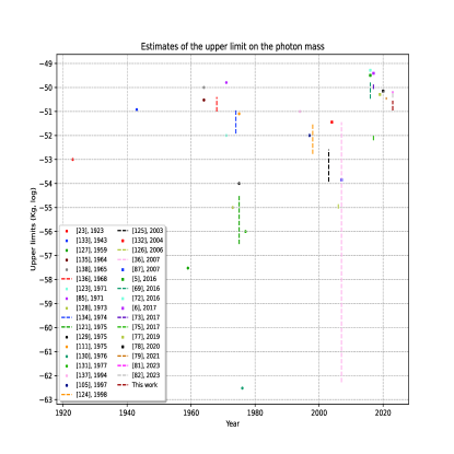
Figure 8: The upper limits listed in Tab. III plotted along the years.

Despite one century of painstaking efforts, we still deal with estimates close to the first value de Broglie (1923). We consider all explorations around and below $10^{-51}$ kg threshold worth of a scrupulous analysis. In the Appendix (IX.3), the Table III 3 and Fig. 8, list and display along the years, photon mass upper limits equal and beyond $10^{-50}$ kg. They include the Particle Data Group (PDG) official value of $2\times 10^{-54}$ kg Ryutov (2007); Workman and the Particle Data Group (2022) and other model-dependent results, some newer than those in the reviews Tu et al. (2005); Accioly et al. (2010); Scharff Goldhaber and Nieto (2010); Spavieri et al. (2011).

V Method and data analysis

For our analysis, we have used the MMS data ^,, contained in the Automated Multi-Dataset Analysis (AMDA), an on-line analysis tool for heliospheric and planetary plasma Génot et al. (2021).

AMDA provides different data, among which we find the ion (electron) densities $n_{i}$ ($n_{e}$), and the velocities ${\vec{v}}_{i}$ (${\vec{v}}_{e}$). We do not take the neutrality condition for granted and compute the plasma current directly in AMDA as ($q$ is the charge)

$${\vec{j}}_{P}=q(n_{i}{\vec{v}}_{i}-n_{e}{\vec{v}}_{e})~{}.$$ (6)

In Cartesian components ($x,y,z$), $j_{P}^{x}=q(n_{i}v_{i}^{x}-n_{e}v_{e}^{x})$ and similarly for $y,z$; the modulus is $j_{P}=\sqrt{(j_{P}^{x})^{2}+(j_{P}^{y})^{2}+(j_{P}^{z})^{2}}$. We computed the error on $j_{P}$ through propagation from the errors on the velocities and densities provided by AMDA Gershman et al. (2015, 2019), and the average of $j_{P}$ for the four spacecraft, considering their errors. For $\Delta j_{P}^{x}\!=\!q\left(v_{i}^{x}\Delta n_{i}+n_{i}\Delta v_{i}^{x}+v_{e}^{x}\Delta n_{e}+n_{e}\Delta v_{e}^{x}\right)$ and similarly for $y,z$, the total error is

$$\Delta j_{P}=\frac{1}{j_{P}}\left(|j_{P}^{x}|\Delta j_{P}^{x}+|j_{P}^{y}|\Delta j_{P}^{y}+|j_{P}^{z}|\Delta j_{P}^{z}\right)~{}.$$ (7)

AMDA provides $j_{B}$, but not its error. Therefore, we have implemented the curlmeter technique Dunlop et al. (1988, 2002) for computing both quantities. We consider a linear approximation of the gradient of the magnetic field measured by the four spacecraft ($\ell=1,2,3,4$). Under this assumption ${\vec{j}}_{B}$ is Chanteur and Mottez (1993)

$${\vec{j}_{B}}=\frac{1}{\mu_{0}}\sum_{\ell=1}^{4}{\vec{k}}_{\ell}\times{\vec{B}}_{\ell}~{},$$ (8)

where ${\vec{k}}_{l}$ are the reciprocal vectors of the tetrahedron, defined by (${\vec{r}}_{ij}={\vec{r}}_{j}-{\vec{r}}_{i}$, where $i$ and $j$ refer to the spacecraft positions)

$${\vec{k}}_{1}= \frac{{\vec{r}}_{23}\times{\vec{r}}_{24}}{{\vec{r}}_{21}\cdot({\vec{r}}_{23}\times{\vec{r}}_{24})},\quad{\vec{k}}_{2}=\frac{{\vec{r}}_{31}\times{\vec{r}}_{34}}{{\vec{r}}_{32}\cdot({\vec{r}}_{31}\times{\vec{r}}_{34})},$$

$${\vec{k}}_{3}= \frac{{\vec{r}}_{24}\times{\vec{r}}_{21}}{{\vec{r}}_{23}\cdot({\vec{r}}_{24}\times{\vec{r}}_{21})},\quad{\vec{k}}_{4}=\frac{{\vec{r}}_{32}\times{\vec{r}}_{31}}{{\vec{r}}_{34}\cdot({\vec{r}}_{32}\times{\vec{r}}_{31})}~{}.$$

The values of ${\vec{j}}_{B}$ found in AMDA compare satisfactorily with our computations. The errors on ${\vec{j}}_{B}$ depend on the uncertainties of the magnetic field and on the separations between the spacecraft. For the former, we consider a constant value $\Delta B=0.1\times 10^{-9}$ T for each component of the magnetic field Torbert et al. (2016). This implies an overall error of $0.17$ nT on the modulus of the magnetic field used in our computations. The fluxgate magnetometer offset determination is achieved after two days of solar wind data Plaschke (2019); for the latter, we consider a relative error equal to $1\%$ of the separation distance Kelbel et al. (2003). From the error propagation, we have found that the error on the $q$ component for a single spacecraft reads as

$$\Delta j_{\ell~{}B}^{q}=(|k_{\ell}^{r}|+|k_{\ell}^{s}|)\Delta B+|B_{\ell}^{r}|\Delta k_{\ell}^{s}+|B_{\ell}^{s}|\Delta k_{\ell}^{r}~{},$$ (9)

$r,s$ being the other components. The final error on the $q\textsuperscript{th}$ component of ${\vec{j}}_{B}^{q}$ is

$$\Delta j^{q}_{B}=\sum_{\ell=1}^{4}\Delta j_{\ell~{}B}^{q}~{}.$$ (10)

The downloaded data were sampled at $1$ for gathering an extended sample while avoiding high frequency contributions. Since the instruments were polled at a higher rate of tens of milliseconds Pollock et al. (2016); Russell et al. (2016), we have verified that AMDA delivers the average of the values belonging to our sampling time, and thus does not pick up a single value each second. Therefore, the high frequency contributions from ${\vec{j}}_{P}$ are cut off, allowing the comparison with the low frequency ${\vec{j}}_{B}$. We have spanned almost six years of measurements, from November 2015 to September 2021, considering only "burst mode" data Fuselier et al. (2016) - data with the highest time resolution collected by MMS. Within this data set, we selected the time intervals

• in which both ${\vec{j}}_{B}$ and ${\vec{j}}_{P}$ are available,

• where the four ${\vec{j}}_{P}$ currents, measured by each spacecraft (including the error bands) overlap, assuring overlapping of the four outputs.

This eases the comparison with ${\vec{j}}_{B}$, supposed to be uniform inside the tetrahedron volume, drawn by the four satellites. We have analysed approximately $3.8\times 10^{6}$ data points, for each of which we have collected 82 physical quantities: the ion and electron component velocities for four spacecraft (24), distances in components between spacecraft (15), barycentre coordinates (3), the electric field at the first spacecraft (3), the electron and ion densities (8), the parallel and perpendicular electron and ion temperatures (16), the magnetic field (12), and the detection time (1).

The displacement current is computed from the ratio of the electric field variation over the sample interval of 1 s. The average of ${\vec{j}}_{E}=1.4\times 10^{-14}$ Am^-2 is six orders of magnitude smaller than the averages of the curl and particle currents and two orders below their smallest difference, Tab. 1. This assures us that its contribution is negligible with respect to the other two currents. We thus compared, at each second, ${\vec{j}}_{B}$ with ${\vec{j}}_{P}$, Eq. (5). We label the comparison ”inconsistency” if there is a gap between the two current bands - nominal values plus/minus the errors from Eqs. (7,10). We stress that these errors are experimental, obtained from the propagation of the reported instrumental uncertainties. According to our approach, we the gap might be attributed to a non-Maxwellian current ${\vec{j}}_{nM}$, Eq. (5) or to an undetected error. A ”consistency” occurs when the two current bands overlap. In these cases, we determine an upper limit to ${\vec{j}}_{nM}$, as the smallest amount to add (subtract) to (from) one of the two currents to arrive at an inconsistency case, Fig. 1. The procedure is

$$|{\vec{j}}_{\rho}|-\Delta|{\vec{j}}_{\rho}|-\left(|{\vec{j}}_{\epsilon}|+\Delta|{\vec{j}}_{\epsilon}|\right)=\Delta{j}\underset{overlap}{\overset{gap}{\gtrless}}0~{},$$ (11)

where $\rho,\epsilon=B,P$ depending on whether $|{\vec{j}}_{P}|-\Delta|{\vec{j}}_{P}|$ is larger or smaller than $|{\vec{j}}_{B}|-\Delta|{\vec{j}}_{B}|$.

This analysis has been carried out for both the modulus and the Cartesian components. In the latter case, an inconsistency is declared if a gap emerges from at least one of the three axes.

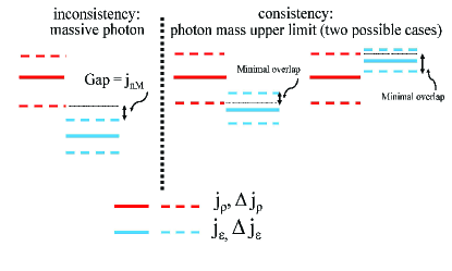
Figure 1: The red (black) and blue (grey) lines represent the currents, and, if dotted, the error bounds. On the left, the case of inconsistency, where the gap implies ${\vec{j}}_{nM}\neq 0$. On the right, the case of consistency, for which moving upward or downward one of the two bands, we would fall in the inconsistency case, finding just an upper limit for ${\vec{j}}_{nM}$. This computation has been carried out for the modulus and for each component.

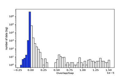
Figure 2: Histogram of Eq. (11) for burst data. Most values are negative (overlaps) in blue (grey) bars, on the left of, and close to, zero. The positive values (gaps), white bars, are on the right of zero, and range from $1.1\times 10^{-12}$ Am^-2 to $1.5\times 10^{-5}$ Am^-2.

Scrutinising the entire data set, we find $2\%$ of inconsistencies for the modulus and $5.2\%$ in Cartesian components; indeed, it may occur that the sum of the currents in absolute values is zero, but their vectorial sum is not, Eq. (5). Such a low number of inconsistencies shoild not be interpreted straightforwardly as a negative outcome of a test on physics foundations, but rather as the consequence of a mission crossing mostly turbulent regions of magnetic reconnection. As later shown, the vast majority of the inconsistencies lay in the solar wind which represents only 14% of the entire data set, Tab. 2. The results of the analysis of Eq. (11) are shown in Figs. 2, 3. It must be added that our analysis considers a large data set of $3.8\times 10^{6}$ points, a large sample size, allowing us to find inconsistencies that might have remained unseen in previous experiments. For the application of the curlmeter technique, the shape of the tetrahedron drawn by the position of the four satellites matters. Since this method is sensitive to the relative separations between the spacecraft Dunlop et al. (2018), we select similar and quasi-optimal configurations. Referring to a regular tetrahedron, we employ the geometrical quality factor Fuselier et al. (2016) on the volume $Q=V_{a}/V_{r}$, where $V_{a}$ is the actual volume of the tetrahedron in a given moment, while $V_{r}$ is the volume of the regular tetrahedron having as side the average of the separations between the spacecraft. We have computed $Q$ for data points and set $Q>0.7$ as a threshold for the high quality geometrical factor. The percentages of inconsistencies slightly increase to $2.2\%$ for the modulus and slightly decrease to $4.8\%$ for the components. For the current means, see Tab. 1.

	$j_{B}$	$\Delta j_{B}$	$j_{P}$	$\Delta j_{P}$
Mean (Gaps)	$4.9\times 10^{-8}$	$6.9\times 10^{-8}$	$2.0\times 10^{-7}$	$5.4\times 10^{-8}$
Mean (Overlaps)	$2.1\times 10^{-8}$	$1.8\times 10^{-7}$	$3.9\times 10^{-8}$	$2.4\times 10^{-8}$

Table 1: The average values [Am^-2] for the currents and their errors, considering the data with $Q>0.7$.

We have localised burst data for associating inconsistencies to physical regions of different levels of turbulence, to understand if the underlying physics of plasma influences the results and ultimately the number of inconsistencies. Various criteria to differentiate the plasma regions, have been proposed, e.g., Rezeau and Belmont (2018), which in our case has led to an often ambiguous assignment of data to regions. We have thus identified the regions otherwise. We have computed the ram $p_{R}$, magnetic $p_{M}$, and thermal $p_{T}$ pressures at each data point. If $p_{R}>10~{}max(p_{M},p_{T})$, we identify the region as solar wind; if $0.3~{}min(p_{M},p_{T})<p_{R}<4~{}max(p_{M},p_{T})$, as magnetosheath; finally, if $10~{}p_{R}<p_{M}$, as magnetosphere. The region of undetermined data points between the solar wind and the magnetosheath is named zone I; between the magnetosheath and magnetosphere, zone II, see Tab. 2. Remarkably, we observe that the gaps (solar wind + zone I), amount to 76% (42473/55916) in modulus and 65% (77847/119850) by components lay in 14% of the total data. This seems to indicate a strong effect of the plasma environmental conditions.

Results	Solar Wind	Zone I	Magnetosheath	Zone II	Magnetosphere
Gaps (M)	$24376$	$18097$	$10669$	2203	$571$
Overlaps (M)	$92190$	$261103$	$1033981$	$356592$	$707595$
Gaps (C)	$34813$	$43034$	$35422$	$5421$	$1160$
Overlaps (C)	$81753$	$236166$	$1009228$	$353374$	$707006$
Data by region/total data	$4.5\%$	$9.5\%$	$42.9\%$	$14.1\%$	$29\%$
Gaps by region/total gaps (M)	$39\%$	$31.1\%$	$24\%$	$4.5\%$	$1.4\%$
Gaps/total data by region (M)	$20.8\%$	$6.4\%$	$1.0\%$	$0.6\%$	$0.1\%$
Gaps/total data by region (C)	$29.7\%$	$15.3\%$	$3.3\%$	$1.5\%$	$0.2\%$

Table 2: Results in modulus (M) and components (C) on gaps (inconsistencies) and overlaps (consistencies) for burst data and $Q>0.7$, analysed by region, in number and percentages.

V.1 Reliability of the analysis

The computation of $j_{P}$ in the solar wind is reliable enough to claim inconsistencies for the following considerations:

1. we have observed the absence of correlations between inconsistencies and particle densities; thus the inconsistencies are not related to systematic effects due to low densities. Indeed, for the solar wind and zone I inconsistencies, the electron density has an average of $22.96$ cm^-3 and a median of $11.88$ cm^-3; the ion density has an average of $22.85$ cm^-3 and a median of $12.1$ cm^-3; only in $13.6\%$ and $8.6\%$ of cases the electron and ion densities, respectively, are smaller than $5$ cm^-3; these values appear sufficient for an adequate measurement of $j_{P}$. For the inconsistencies in all regions, we add that

2. $j_{P}$ is larger than $j_{B}$ in 95.6% of the cases; were the uncertainties provided by AMDA not representative of all sorts of errors, the following cases may arise:

   1. $j_{P}$ is underestimated; this case would not matter: if we had we the ’real’ $j_{P}$, its difference with $j_{B}$ would increase and the gap would be deeper;

   2. $j_{P}$ is overestimated; this case may lead to:

      1. lower the number of inconsistencies but also reduce the differences between the two currents and thereby the photon mass, for a given potential (a positive result for our study); or

      2. cancel inconsistencies, but this case would be statistically compensated by the 2.(a) and 2.(b).i cases;

3. we derive a single $j_{P}$ by averaging the currents of the four spacecraft, only when the four error bands overlap; by this procedure, we reduce the effect of a possible calibration error.

We stress that we are more interested in assessing the differences between currents rather than evaluating them exactly.

V.2 The potential

The current differences are strictly the outcome of experimental data, but an estimate of the potential is mandatory to deal with the photon mass (upper limit), Eq. (1). We focus on the solar wind for the following reasons: i) most inconsistencies lay in this region; ii) comparison with other existing model-based Ryutov (1997) and experiment-based limits Retinò et al. (2016), derived in this region; iii) the determination of the vector potential in the magnetosheath and magnetosphere is computationally cumbersome Romashets et al. (2008); Romashets and Vandas (2008) and it deserves a separate work. We use the analytical computation, based on the Parker model, of $|{\vec{A}}|$ in the Coulomb gauge Bieber et al. (1987) at each data point. The potential, in spherical coordinates and in the Coulomb gauge, is

$$A_{r}=\frac{2b}{3}\biggr{[}1-\frac{3}{2}x-x\ln{(1+x)}\biggl{]}~{},$$ (12)

$$A_{\theta}=\frac{2b}{3}\sin\theta\biggr{[}\frac{x}{1+x}+\ln(1+x)\biggr{]}\biggr{(}\frac{\cos\theta}{x}\biggl{)}~{},$$ (13)

$$A_{\phi}=\frac{a}{r\sin\theta}(1+x)~{},$$ (14)

where $x=|\cos\theta|$ and, at 1 AU and for magnetic fields equal to 5   nT, $a=3.54\times 10^{-9}$ T AU², $b=3.54\times 10^{-9}$ T AU. Near the Earth for the modulus of the potential, a direct proportionality emerges, that is $A=\sqrt{11/6}~{}BR$, where $R$ is 1 AU.

For the adoption of the Coulomb gauge, we recall that for deriving the dBP equations from the Lagrangian, we impose the Lorenz condition. If the scalar potential is (almost) time independent, then the Coulomb and Lorentz conditions can be considered equivalent.

VI Upper limits

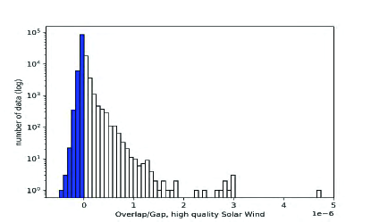
Figure 3: Histogram of Eq. (11) for burst data ($Q>0.7$) in the solar wind. Most values are negative (overlaps) in blue (grey) bars, on the left of, and close to, zero. The positive values (gaps), white bars, are on the right of zero, and range from $2.0\times 10^{-12}$ Am^-2 to $4.7\times 10^{-6}$ Am^-2.

We can infer an upper bound of the photon mass. The found distributions are strongly asymmetric and thus the standard deviation on the mean measurement would be misleading.

We threat the data concerning the inconsistencies (gaps) and consistencies (overlaps) in a singular statistical analysis. We restrict our analysis to the values shown in Fig. 3, and use this expression

$$m_{\gamma}=\frac{\hbar{\sqrt{\mu_{0}}}}{c}\sqrt{\displaystyle\frac{|\Delta{\vec{j}}|}{|{\vec{A}}|}}~{}{\rm~{}kg}~{},$$ (15)

which we can compute in the solar wind.

For the analysis of the entire data set we refer to the definitions in Fig. 1, recalling that the consistencies are defined as negative, while the inconsistencies are positive. From Fig. 3, we compute the median and the $25\%$ and $75\%$ percentiles, in order to find a proper confidence interval for our results.

We consider the modulus of the consistencies to assess the upper bound of the photon mass from our analysis of the entire set of data. We find a median value equal to $2.7\times 10^{-8}$ Am^-2, with a $25\%$ percentile equal to $7.9\times 10^{-9}$ Am^-2 and a $75\%$ percentile of $4.7\times 10^{-8}$ Am^-2.

Having computed also the median for the potential in the solar wind data, $1.8\times 10^{3}$ T m, we derive an estimate equal to $2.1\times 10^{-51}$ kg, with a confidence interval going from $1.1\times 10^{-51}$ kg to $2.8\times 10^{-51}$ kg. This upper limit levels to the recent observational estimates derived by FRB.

For the LSV parameter $|\vec{k}^{\rm AF}|$, Eq. (3), the median is $6\times 10^{-9}$ m^-1, for $\theta=1$, in line with laboratory upper limits.

VII The question of the inconsistencies in the solar wind

After having found the upper limits, we now focus on the inconsistencies jn the solar wind.

In this section, we suppose that the inconsistencies (gaps) in the solar wind are manifestations of non-standard electro-magnetic effects, Eq. (15), and not of unaccounted experimental errors. In other words, we reverse the ordinary thinking and see if the found mass value is compatible with existing upper limits. The objective is not claiming a photon mass discovery, but rather emphasising that the evidence of the masslessness of the photon at the $10^{-53}$ kg level is worthy a scrupolous analysis. Therefore, we proceed by i) addressing the solar wind, ii) analysing the official limit in the literature, iii) examining our results in the solar wind regime.

The nature of the solar wind.

We refer to the nearly collisionless nature of the solar wind implying that the mean free path of the particles is in of the order of 1 AU Sahraoui et al. (2020). Thereby, the kinetic energies and momenta of the particles change only as a result of the averaged fields generated by the other particles. How turbulence explains the acceleration of plasma particles, i.e. the transfer of energy across a broad range of scales that leads to complex chaotic motions, structure formation and energy conversion, is a marginally pertinent for this work. Indeed, the solar wind flows rapidly towards Earth carrying the solar magnetic field. When it smacks right into the terrestrial magnetic field, it generates the bow shock and the current flow becomes turbulent. Until then, the solar wind is possibly the least troublesome region for testing the AM law. Thus, the region of the solar wind before the shock presents the best conditions to test the AM law.

Comparison with the literature.

We discuss the PDG Workman and the Particle Data Group (2022) adopted limits coming out of modelling the solar wind magnetohydro-dynamics at 1 AU Ryutov (1997) and later at 40 AU Ryutov (2007). In Ryutov (1997), the extensive application of the Parker model Parker (1958) couples to the absence of data and of error analysis. The final estimate is based on reconciling theory with the non-observation of large plasma motions in the solar wind. There is not an actual upper limit being stated, but a supposed improvement of a factor of 10 with reference to a differently obtained estimate Davis jr. et al. (1975) which concerns Jupiter data at 5.2 AU.

The $1.4\times 10^{-54}$ kg limit Ryutov (2007). stands as the actual official upper limit. As the former, it is based entirely on the Parker model, on a qualitative reasoning ad absurdum, while data are not presented and an error analysis is absent.: the estimated feebleness of the ${\vec{j}}\times{\vec{B}}$ force and the absence of deceleration of the radial expansion at Pluto orbit. But recent results Elliott et al. (2019) have conversely shown that the solar wind slows down reaching Pluto. The final estimate, Eq. (14) in Ryutov (2007), comes from a single set of three data: magnetic field, ion density and particle velocity, taken from the missions Pioneer and Voyager; if these values were to vary of just $70\%$ - as it may easily happen - the limit would worsen of one order of magnitude.

Our comments aim solely to show the shortcoming of a legitimate, but model-based upper limit.

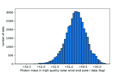
Figure 4: For the solar wind and zone I regions burst data and $Q>0.7$, the histogram of the dBP photon mass derived from the inconsistencies, supposing that the latter are not associated with unaccounted errors. The the median of the distribution is $2.5\times 10^{-51}$ kg, which is a close value to the previously presented upper limit.

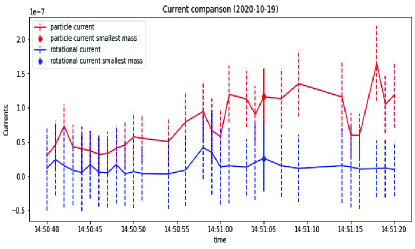
Figure 5: Supposing that all errors have been considered, the smallest dBP photon mass, see the spots, occurs on 19 October 2020, at 14h 51m 05s, in the zone I burst data and $Q=0.82$. The particle current $j_{P}=(1.2\pm 0.4)\times 10^{-7}$ Am^-2, and the rotational current $j_{B}=(2.6\pm 4.9)\times 10^{-8}$ Am^-2 produced a difference of $7.4\times 10^{-12}$ Am^-2. This difference is not visible on the vertical axis carrying units which are five orders of magnitude larger. The vertical dotted lines are the errors. The potential of $3.8\times 10^{3}$ T m leads to a mass of $1.7\times 10^{-53}$ kg, Eq. (15), and thereby $|\vec{k}^{\rm AF}|=5\times 10^{-11}$ m^-1, Eq. (3).

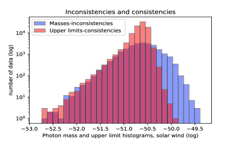
Figure 6: For the solar wind region burst data and $Q>0.7$, the histograms of the dBP photon mass upper limits derived from the consistencies and the dBP photon mass values derived from the inconsistencies, supposing that the latter are not associated to unaccounted errors. Only the inconsistencies in absolute value are shown, representing 20.8% of the total data in the region. We recall that the inconsistencies in components are 29.7% in the region.

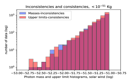
Figure 7: Same caption of the previous figure. The values below $10^{-51}$ kg are zoomed in.

Deviations from the Ampère-Maxwell law.

Figure 4, displays the dBP photon mass estimates from the inconsistencies. We learn that: i) the median for solar wind and zone I is $1.8\times 10^{-51}$ kg, which is close to the value of the photon mass upper limit; ii) if we mean by minimum the mass value that would fit all inconsistency cases, this would be $1.7\times 10^{-53}$ kg.

Incidentally, since the potential is space-time dependent, the minimum photon mass does not necessarily correspond to the minimum current deviation, $7.4\times 10^{-12}$ Am^-2, Fig. 5.

In Figs. 6, 7, we show the two distributions of overlaps and gaps. They look very similar, due to our definition of the upper limit, involving the minimum displacement, upward or downward, of the current bands, Fig. 1. Indeed, the two distributions almost overlap, especially for values of mass upper limits and the dBP photon mass below $10^{-51}$ kg, Fig. 7. In this domain the percentages of inconsistencies arrive up to 45.2%.

The similarity of the distributions for weak current differences in the solar wind warns against all attempts of using oversimplified models.

Table III shows that around $10^{-53}$ kg level and beyond, there is crowding of model-based limits.

VIII Discussion, conclusions, perspectives

Considering the entire set of consistencies and inconsistencies in the solar wind, we found an estimate on the upper bound for the photon mass equal to $2.1\times 10^{-51}$ kg, and for the LSV parameter $|\vec{k}^{\rm AF}|$, which is $6\times 10^{-9}$ m^-1. The photon mass upper limit is consistent with various other upper limits found from recent FRB observations, Tab. III, while the LSV upper limit is compliant with terrestrial experiments Gomes and Malta (2016).

After error analysis, we have found deviations from the AM law in 2.2% of the cases for the modulus and 4.8% for the vector components. Such a paucity of cases turns into a large minority if the burst modes are counted only in the solar wind. We then find inconsistencies in 20.8% of the cases for the modulus and 29.7% for the components.

The identification of numerous deviations from the AM law might be related to our analysis encompassing a large data set of $3.8\times 10^{6}$ points, allowing us to uncover inconsistencies that might have remained undetected in earlier studies.

We lack experimental constraints to definitively rule out a mass at $10^{-53}$ level, Tab. III. Many published limits are identified as speculative Workman and the Particle Data Group (2022). Ref. Scharff Goldhaber and Nieto (2010) states ”Quoted photon-mass limits have at times been overly optimistic in the strengths of their characterizations. This is perhaps due to the temptation to assert too strongly something one knows to be true”.

Although we find deviations from Ampère-Maxwell law for some data points, we do not intend to claim it as the final result. We cannot exclude possible mismatches between currents, even after instrument calibration and analysis of systematic effects on MMS Gershman et al. (2015); Fuselier et al. (2016); Pollock et al. (2016); Russell et al. (2016); Gershman et al. (2019), as the intrinsic charge Barrie et al. (2019). Reducing systematic errors to a minimum is an objective for MMS. The instrumentation enables regular cross-calibration and validation of the Field Plasma Investigation (FPI) data, reducing systematic errors to within a few percent, thus providing suitable accuracy to calculate the current directly from particle observations Gershman et al. (2019). For the Digital Flux Gate (DFG) and the Analogue Flux Gate (AFG) magnetometers, the ground calibration is refined in space to ensure all eight magnetometers are precisely inter-calibrated Russell et al. (2016).

The values of the upper limit of distribution are similar to the values of the photon mass inferred from the inconsistencies distribution due to our rigorous definition of the upper limit, involving the minimum displacement, upward or downward, of the current bands.

Summarising, our main result is not the upper limit on the photon mass, nor do we claim to have found a massive photon. Our main result is having found numerous inconsistencies (up to 30%) in the best sub-set of data (in the solar wind, which is the best for our investigation since it possibly corresponds to the least turbulent region Neugebauer (1976) crossed by MMS). These inconsistencies are likely due to unknown experimental errors, but we cannot exclude non-Maxwellian terms. The preceding should be seen in the context of a non-dedicated mission, since the aforementioned ’best data’ set is only five percent of the 3.8 million data. Still, even if we consider only this subset, the number of data analysed is enormous when compared to qualitative assessments based on models and on one single set of values.

The determination of the nature of the deviations is a challenge that requires exploring current differences well below $10^{-11}$ Am^-2, Eq. (15), ideally four orders of magnitude, to reach the $10^{-55}$ kg area. While this is ambitious, it paves the way to new and far reaching, combined explorations in plasma and fundamental physics, which are usually separated domains of research. The accuracy in measuring the velocity difference of ions and electrons $v_{i}-v_{e}=(\Delta j+j_{B})/qn$ in the order of $1.5\times 10^{4}$ ms^-1 is technologically feasible, conversely to Cluster, where $j_{B}\ll j_{P}$ led to $10^{-4}$ ms^-1 as required velocity difference Retinò et al. (2016). Since the curlmeter method does not allow to estimate currents in regions smaller than the scale of the tetrahedron itself, a constellation of more than four spacecraft targeting the solar wind with high quality data would be desirable. Indeed, future satellite measurements may clarify the nature of the deviations, whether unaccounted errors or profoundly meaningful first glimpses of new physics. Despite the growing gravitational astronomy, photons remain our main tool for interpreting the Universe. Being herein confronted with a non-dedicated mission to fundamental physics, we urge to not spare efforts to explore the foundations of physics.

Acknowledgements.

CNES and the Federation Calcul Scientifique et Modélisation Orléans Tours (CaSciModOT) for missions and the student internships of S. Dahani and A. Gauthier are thanked. Discussions with G. Chanteur, H. Breuillard and A. Retinò (Paris), V. Génot (Toulouse), D. Gershman (NASA), B. Lavraud (Bordeaux), A. Vaivads (Stockholm), E. Vitagliano (Los Angeles) and the colleagues T. Dudok de Wit, P. Henri, V. Krasnosselskikh, J.-L. Pinçon (Orléans) are acknowledged. GS thanks the hospitality of LPC2E, the support by the Istituto Nazionale di Fisica Nucleare, Sez. di Napoli, Iniziativa Specifica QGSKY and the Erasmus+ programme.

IX Appendix

IX.1 The Proca conception of the photon

Proca conjectured that the photon would be composed of two pure charge massless particles, one positive and one negative. The Lagrangian in Proca’s original notation is Proca (1936, 1937)

$${\cal L}=h^{2}c^{2}\left[\frac{1}{2}F_{rs}G_{rs}+k^{2}\psi^{*}_{r}\psi_{r}\right]~{},$$ (16)

where $F_{rs}=(\partial_{r}+iA_{r})\psi_{s}^{*}-(\partial_{s}+iA_{s})\psi_{r}^{*}$ and $G_{rs}=(\partial_{r}-iA_{r})\psi_{s}-(\partial_{s}-iA_{s})\psi_{r}$ are tensorial fields; $A_{s}=e\phi_{s}/hc$, being $e$ the charge, $h$ the Planck constant, $c$ the light speed and $\phi$ the field potential; $\psi$ is a wave-function (vecteurs d’univers) and $k=mc/h$. Proca affirmed that for photons $\psi^{*}_{r}=\psi_{r}$ and $m=0$.

IX.2 The question of mass and damping in the SME

Frame dependency is unusual for mass, but similarly to the non-covariance of energy in general relativity, we should not be refrained from using the concept of mass. What distinguishes an effective from a physical mass? Massless particles such as charged leptons, quarks, W, and Z Bosons acquire mass through the Higgs mechanism, while composite hadrons (baryons and mesons) from Chiral Symmetry (Dynamical) Breaking (CSB). How to qualify the mass induced by LSV? In Quantum Field Theory (QFT), a physical mass is a quantity calculated perturbatively by considering loop effects and computing the poles of the loop-corrected propagators. Since the CFJ term respects gauge symmetry and there is no room for anomalies in the model, loop corrections do not shift the pole of the tree-level propagator. This implies that the mass may be interpreted both effective and physical.

For the CPT-odd handedness, ${k}^{\rm AF}_{0}$ and $\vec{k}^{\rm AF}$ are the time and space components of ${k}^{\rm AF}$ $\left({k}^{\rm AF}_{0},\vec{k}^{\rm AF}\right)$. For

$$\begin{cases}&\bar{\omega}=\omega/c~{},\\ &k^{\mu}=\left(\bar{\omega},\vec{k}\right)~{},\\ &k^{2}=\bar{\omega}^{2}-|\vec{k}|^{2}~{},\\ &\left(k^{\rm AF}_{\mu}k^{\mu}\right)^{2}=\left(k^{\rm AF}_{0}\bar{\omega}-{\vec{k}}^{\rm AF}\cdot{\vec{k}}\right)^{2}~{},\end{cases}$$ (17)

the CFJ dispersion relations at fourth order in the 4-momentum $k$ Bonetti et al. (2017c); Bonetti et al. (2018), originally in Carroll et al. (1990), are

$$k^{4}+({k}^{\rm AF})^{2}k^{2}-({k}^{\rm AF}\cdot k)^{2}=0=$$

$$\left(\bar{\omega}^{2}\!-\!\vec{k}^{~{}2}\right)^{2}\!\!+\!\left[\left({k}^{\rm AF}_{0}\right)^{2}\!\!-\!\left({\vec{k}}^{\rm AF}\right)^{2}\right]\left[\bar{\omega}^{2}\!-\!\vec{k}^{~{}2}\right]\!-\!\left({k}^{\rm AF}_{0}\bar{\omega}\!-\!{\vec{k}}^{\rm AF}\!\cdot{\vec{k}}\right)^{2}$$ (18)

We consider three cases.

Case 1. Taking ${\vec{k}}=0$, Eq. (18) becomes

$$\bar{\omega}^{2}\left[\bar{\omega}^{2}-({\vec{k}}^{\rm AF})^{2}\right]=0~{}.$$ (19)

The roots are $\bar{\omega}=\left(0,|{\vec{k}}^{\rm AF}|\right)$, for any value of $k^{\rm AF}_{0}$. Zero momentum does not forcefully imply zero photon energy, unless ${k}^{\rm AF}$ is purely time-like. But time-likeness causes a problem with the unitarity of the quantum version of this theory Adam and Klinkhamer (2001).

Case 2. We now consider $k^{\rm AF}_{0}=0$. Eq. (18) becomes

$$\bar{\omega}^{4}-\left[\left({\vec{k}}^{\rm AF}\right)^{2}+2{\vec{k}}^{~{}2}\right]\bar{\omega}^{2}+\left[\left({\vec{k}}^{\rm AF}\right)^{2}{\vec{k}}^{~{}2}-\left({\vec{k}}^{\rm AF}\cdot{\vec{k}}\right)^{2}+{\vec{k}}^{4}\right]=0~{}.$$ (20)

The roots are $\bar{\omega}^{2}={\vec{k}}^{~{}2}+\frac{1}{2}\left({\vec{k}}^{\rm AF}\right)^{2}\pm\frac{1}{2}\sqrt{\left({\vec{k}}^{\rm AF}\right)^{4}+4\left({\vec{k}}^{\rm AF}\cdot{\vec{k}}\right)^{2}}$

Case 3. If as for Case 2, $k^{\rm AF}_{0}=0$ but also ${\vec{k}}^{\rm AF}\cdot{\vec{k}}=0$, the roots simplify to $\bar{\omega}^{2}=\left[{\vec{k}}^{~{}2},{\vec{k}}^{~{}2}+\left({\vec{k}}^{\rm AF}\right)^{2}\right]$ . Here, the second set of roots reminds of the dBP dispersion relation.

In addition to the above demonstration, other arguments for the massiveness of the photon can be put forward. Before doing so, we remind that the number of polarisations is depending on our gauge choice which depends on our assumptions and on the experimental evidence.

• For a massless photon, the longitudinal polarisation is forbidden since it implies that the photon would travel at $v<c$ (due to the vibrations in the direction of motion), while in the massive case, there is compatibility.

• The CFJ Lagrangian was rewritten Bonetti et al. (2017c) to display a term $|\vec{k}^{\rm AF}|~{}A_{i}A^{i}$, $A_{i}$ being the four-potential as in the dBP Lagrangian. Electro-dynamics models exhibiting this term have a modified constraint algebra due to the gauge symmetry breaking Errasti Díez et al. (2020). This causes the propagation of an additional degree of freedom, leading to a total of three.

• As already stated, in Baêta Scarpelli et al. (2003, 2004), it was shown that a LoSy breaking includes a massive mode in the propagator proportional to the violation vector.

• In vacuo, while $\nabla{\vec{B}}$ remains zero, this is not the case anymore for $\nabla{\vec{E}}$. The energy-momentum relation that emerges as a dispersion relation neatly points out the presence of a mass, much in the way of a Klein-Gordon dispersion relation.

• The Higgs mechanism does not forbid the creation of a photon mass, also in the LSV context Itzykson and Zuber (2006); Adelberger et al. (2007).

• It has been shown Altschul (2006), that by computing the radiative correction of the photon self-energy, two masses may arise. In the pure time-like case, photons assume a tachyonic behaviour.

• In Altschul (2006) the Fermionic sector induces a photon mass through the LSV. In our work Bonetti et al. (2017c); Bonetti et al. (2018), the CFJ term is already included in the model and we don’t need to step back to the Fermionic origins. In this sense, our work Bonetti et al. (2017c); Bonetti et al. (2018) may be considered Altschul (2006).

In the SME framework, damping is a complex issue. A purely time-like $k^{\rm AF}$ vector was considered Altschul (2014); Schober and Altschul (2015, 2016), despite the issue of unitarity Adam and Klinkhamer (2001). In the last of these references, the divergence of $\vec{E}$ is zero, whereas the curl of $\vec{B}$ differs from the corresponding Maxwellian form. Therefore the long-distance behaviour of the electric and magnetic field differs. The same reference states that there are important differences between time-like and space-like cases.

Indeed, the damping for the space-like case is the same for both electric $\vec{E}$ and magnetic $\vec{B}$ fields as their Green functions share the same poles, regardlessly of the kind of source, in the static cases, see below. Nevertheless, even if the damping is identical, the coupling of the perturbation vector with the ${\vec{E}}$ and ${\vec{B}}$ fields, in the Gauss and AM laws, determines a direction-dependent damping.

Damping for electric and magnetic fields, for a space-line perturbation vector $k^{\rm AF}$.

In a static regime, for whatever source and in absence of a current, the wave equations for the potentials $\phi$ and $\vec{A}$ read as follows

$$\left[\left(\nabla^{2}\right)^{2}-\left({\vec{k}}^{\rm AF}\right)^{2}\nabla^{2}+\left({\vec{k}}^{\rm AF}\cdot\vec{\nabla}\right)^{2}\right]\phi=-\nabla^{2}\frac{\rho}{\epsilon_{0}}-\mu_{0}c\left.\right.{\vec{k}}^{\rm AF}\cdot\left(\vec{\nabla}\times\vec{j}\right)$$ (21)

$$\left\{\left[\left(\nabla^{2}\right)^{2}-\left({\vec{k}}^{\rm AF}\right)^{2}\nabla^{2}+\left({\vec{k}}^{\rm AF}\cdot\vec{\nabla}\right)^{2}\right]\delta_{ij}+\left({\vec{k}}^{\rm AF}\right)^{2}\partial_{i}\partial_{j}+k^{\rm AF}_{i}k^{\rm AF}_{j}\nabla^{2}-\left({\vec{k}}^{\rm AF}\cdot\vec{\nabla}\right)\left(k^{\rm AF}_{i}\partial_{j}+k^{\rm AF}_{j}\partial_{i}\right)\right\}A_{j}=\frac{1}{\epsilon_{0}c}\left({\vec{k}}^{\rm AF}\times\vec{\nabla}\rho\right)_{i}-\left(\mu_{0}\nabla^{2}\vec{j}\right)_{i}$$ (22)

By using the AM law, we get the following relation in Fourier space

$$\vec{\tilde{A}}({\vec{k}})=-\frac{1}{c}\frac{1}{k^{2}}{\vec{k}}^{\rm AF}\times\vec{\tilde{E}}({\vec{k}})$$ (23)

This in turn will give for the electric and magnetic fields the following expressions in the case of a static point-like charge $q$

$$\phi=\frac{q}{\epsilon_{0}}\int\frac{d^{3}\vec{k}}{(2\pi)^{3}}\frac{1}{{\vec{k}}^{2}+\left({\vec{k}}^{\rm AF}\right)^{2}-\left({\vec{k}}^{\rm AF}\cdot\hat{k}\right)^{2}}e^{-i\vec{k}\cdot\vec{x}}$$ (24)

$$\vec{E}=-\vec{\nabla}\phi=\frac{q}{\epsilon_{0}}\int\frac{d^{3}\vec{k}}{(2\pi)^{3}}\frac{i\vec{k}}{{\vec{k}}^{2}+\left({\vec{k}}^{\rm AF}\right)^{2}-\left({\vec{k}}^{\rm AF}\cdot\hat{k}\right)^{2}}e^{-i\vec{k}\cdot\vec{x}}$$ (25)

$$\vec{B}=\frac{1}{c}\frac{1}{{\nabla}^{2}}\vec{\nabla}\times({\vec{k}}^{\rm AF}\times\vec{E})=\frac{-q}{c\epsilon_{0}}\int\frac{d^{3}\vec{k}}{(2\pi)^{3}}\frac{{\vec{k}}^{\rm AF}-({\vec{k}}^{\rm AF}\cdot\hat{k})\hat{k}}{{\vec{k}}^{2}+\left({\vec{k}}^{\rm AF}\right)^{2}-\left({\vec{k}}^{\rm AF}\cdot\hat{k}\right)^{2}}e^{-i\vec{k}\cdot\vec{x}}~{}.$$ (26)

The damping in the fields is fixed by the poles of the integrands, which share a common denominator. According to Eqs. (25,26), there are two poles, common to both the integrals, and they are purely imaginary: $i|{\vec{k}}^{AF}|[\sin\alpha|$ and $-i|{\vec{k}}^{AF}||\sin\alpha[$, where $\alpha$ is the angle between ${\vec{k}}^{AF}$ and ${\vec{k}}$. As usual, these integrals may be calculated in complex plane. Since the ${\vec{E}}$ and ${\vec{B}}$ fields should go to zero at infinity, only the pole $-i|{\vec{k}}^{AF}||\sin\alpha|$ is retained. Thus, for a space-like background, the electro-static and magneto-static fields exhibit the same spatial damping, contrary to what happens for a time-like $k^{AF}_{\mu}$.

IX.3 Upper limits

Smallest (Heisenberg) measurable mass for any particle is $1.3\times 10^{-69}$ kg for $\Delta t$ = age of the Universe.
Reference	Value ​(kg)	Method
Barnes and Scargle (1975)	$3\times 10^{-57}\newline 3\times 10^{-56}$	Observations of the Crab Nebula magnetohydro-dynamic waves
Ryutov (2007)	$1.4\times 10^{-54}$	Model of the solar wind magnetohydro-dynamics (40 AU) Official PDG limit.
de Bernadis et al. (1984)	$2.9\times 10^{-54}$	Cosmic background dipole anisotropy
de Broglie (1923)	$10^{-53}$	Dispersion
Yang and Zhang (2017)	$6.3\times 10^{-53}\newline 9.6\times 10^{-53}$	Observations of pulsar spin-down
Ryutov (1997)	$10^{-52}$	Model of the solar wind magnetohydro-dynamics (1 AU).
Franken and Ampulski (1971)	$10^{-52}$	Low frequency resonance circuits
Lakes (1998); Luo et al. (2003); Tu et al. (2006)	$9\times 10^{-56}\newline 3.3\times 10^{-52}$	Torsion pendulum
Yamaguchi (1959); Byrne and Burman (1973, 1975); Chibisov (1976); Byrne (1977); Adelberger et al. (2007)	$3\times 10^{-63}\newline 3.6\times 10^{-52}$	Model of the galactic potential
Füllekrug (2004)	$3.6\times 10^{-52}$	Speed of lightning discharges in the troposphere
Davis jr. et al. (1975)	$8\times 10^{-52}$	Satellite data of Jupiter magnetic field
Schrödinger (1943)	$1.2\times 10^{-51}$	Earth and Sun magnetic fields
Hollweg (1974)	$1.1\times 10^{-52}\newline 1.3\times 10^{-51}$	Model of Alfvén waves in the interplanetary medium
This work	$1.1\times 10^{-51}\newline 2.8\times 10^{-51}$	AM law via MMS satellite data
Gintsburg (1964); Goldhaber and Nieto (1968); Fischbach et al. (1994)	$10^{-51}\newline 4\times 10^{-51}$	Earth magnetic field with (satellite) observational data
Retinò et al. (2016)	$3.4\times 10^{-51}\newline 1.6\times 10^{-50}$	AM law via Cluster satellite data
Williams et al. (1971)	$1.6\times 10^{-50}$	Laboratory test on Coulomb’s law
Patel (1965)	$10^{-50}$	Model of Alfvén waves in the Earth magnetic field.
Bonetti et al. (2016); Wu et al. (2016); Bonetti et al. (2017b); Shao and Zhang (2017); Yang and Zhang (2017); Xing et al. (2019); Wei and Wu (2020); Wang et al. (2021); Lin et al. (2023); Wang et al. (2023)	$3.1\times 10^{-51}\newline 5.2\times 10^{-50}$	Fast Radio Bursts

Table 3: Summary of the main photon mass upper limits at and below $10^{-50}$ kg. For full reviews, see Tu et al. (2005); Accioly et al. (2010); Scharff Goldhaber and Nieto (2010); Spavieri et al. (2011); Wei and Wu (2021); Workman and the Particle Data Group (2022).

References

- Kostelecký and Mewes (2009) V. A. Kostelecký and M. Mewes, Phys. Rev. D 80, 015020 (2009), eprint arXiv:0905.0031 [hep-ph].
- Li et al. (2015) S. Li, J. Xia, M. Li, H. Li, and X. Zhang, Astrophys. J. 799, 211 (2015), eprint arXiv:1405.5637 [astro-ph.CO].
- Mosquera Cuesta and Salim (2004) H. J. Mosquera Cuesta and J. M. Salim, Astrophys. J. 608, 925 (2004), eprint arXiv:astro-ph/0307513.
- Bonetti et al. (2017a) L. Bonetti, S. E. Perez Bergliaffa, and A. D. A. M. Spallicci, in 14th Marcel Grossmann Meeting, edited by M. Bianchi, R. T. Jantzen, and R. Ruffini (World Scientific, Singapore, 2017a), vol. Part D, p. 3531, 12-18 July 2015 Roma, eprint arXiv:1610.05655 [astro-ph.HE].
- Bonetti et al. (2016) L. Bonetti, J. Ellis, N. E. Mavromatos, A. S. Sakharov, E. K. Sarkisian-Grinbaum, and A. D. A. M. Spallicci, Phys. Lett. B 757, 548 (2016), eprint arXiv: 1602.09135 [astro-ph.HE].
- Bonetti et al. (2017b) L. Bonetti, J. Ellis, N. E. Mavromatos, A. S. Sakharov, E. K. Sarkisian-Grinbaum, and A. D. A. M. Spallicci, Phys. Lett. B 768, 326 (2017b), eprint arXiv:1701.03097 [astro-ph.HE].
- Veske et al. (2021) D. Veske, Z. Márka, I. Bartos, and S. Márka, Astrophys. J. 908, 216 (2021), eprint arXiv:2010.04162 [astro-ph.HE].
- Donner et al. (2019) J. Y. Donner, J. P. W. Verbiest, C. Tiburzi, S. Oslowski, D. Michilli, M. Serylak, J. M. Anderson, A. Horneffer, M. Kramer, J. Grießmeier, et al., Astron. Astrophys. 624, A22 (2019), eprint arXiv:1902.03814 [astro-ph.GA].
- Antoniadis et al. (2023) J. Antoniadis, P. Arumugam, S. Arumugam, S. Babak, M. Bagchi, A. Bak Nielsen, C. G. Bassa, A. Bathula, A. Berthereau, M. Bonetti, et al., Astron. Astrophys. 678, A50 (2023), eprint arXiv:2306.16214 [astro-ph.HE].
- Bentum et al. (2017) M. J. Bentum, L. Bonetti, and A. D. A. M. Spallicci, Adv. Space Res. 59, 736 (2017), eprint arXiv:1607.08820 [astro-ph.IM].
- Piórkowska-Kurpas (2022) A. Piórkowska-Kurpas, Universe 8, 83 (2022).
- J. A. Helayël-Neto and Spallicci (2019) J. A. Helayël-Neto and A. D. A. M. Spallicci, Eur. Phys. J. C 79, 590 (2019), eprint arXiv:1904.11035 [hep-ph].
- Spallicci et al. (2021) A. D. A. M. Spallicci, J. A. Helayël-Neto, M. López-Corredoira, and S. Capozziello, Eur. Phys. J. C. 81, 4 (2021), eprint arXiv: 2011.12608 [astro-ph.CO].
- Spallicci et al. (2022a) A. D. A. M. Spallicci, G. Sarracino, and S. Capozziello, Eur. Phys. J. Plus 137, 253 (2022a), eprint arXiv:2202.02731 [astro-ph.CO].
- Sarracino et al. (2022) G. Sarracino, A. D. A. M. Spallicci, and S. Capozziello, Eur. Phys. J. Plus 137, 1386 (2022), eprint arXiv:2211.11438 [astro-ph.CO].
- López-Corredoira and Calvi-Torel (2022) M. López-Corredoira and J. I. Calvi-Torel, Int. J. Mod. Phys. D 31, 2250104 (2022), eprint arXiv:2207.14688 [astro-ph.CO].
- Kouwn et al. (2016) S. Kouwn, P. Oh, and C.-G. Park, Phys. Rev. D 93, 083012 (2016), eprint arXiv:1512.00541 [astro-ph.CO].
- Landim (2020) R. G. Landim, Eur. Phys. J. C 80, 913 (2020), eprint arXiv:2005.08621 [astro-ph.CO].
- Fabbrichesi et al. (2021) M. Fabbrichesi, E. Gabrielli, and G. Lanfranchi, The Physics of the Dark Photon: a Primer, SpringerBriefs in Physics (Springer Nature, Cham, 2021), ISBN 978-3-030-62518-4.
- Caputo et al. (2021a) A. Caputo, A. J. Millar, C. A. J. O’Hare, and E. Vitagliano, Phys. Rev. D 104, 095029 (2021a), eprint arXiv:2105.04565 [hep-ph].
- Caputo et al. (2021b) A. Caputo, S. J. Witte, D. Blas, and P. Pani, Phys. Rev. D 104, 043006 (2021b), eprint arXiv:2102.11280 [hep-ph].
- Cuzinatto et al. (2017) R. R. Cuzinatto, E. M. de Morais, L. G. Medeiros, C. Naldoni de Souza, and B. M. Pimentel, Europhys. Lett. 118, 19001 (2017), eprint arXiv:1611.00877 [astro-ph.CO].
- de Broglie (1923) L. de Broglie, Comptes Rendus Hebd. Séances Acad. Sci. Paris 177, 507 (1923).
- Proca (1936) A. Proca, J. Phys. et Radium 7, 347 (1936).
- Proca (1937) A. Proca, J. Phys. et Radium 8, 23 (1937).
- de Broglie (1936) L. de Broglie, Nouvelles Recherches sur la Lumière, vol. 411 of Actualités Scientifiques et Industrielles (Hermann & Cie, Paris, 1936).
- de Broglie (1940) L. de Broglie, La Mécanique Ondulatoire du Photon. Une Nouvelle Théorie de la Lumière (Hermann & Cie, Paris, 1940).
- de Broglie (1950) L. de Broglie, J. Phys. et Radium 11, 481 (1950).
- Bopp (1940) F. Bopp, Ann. Phys. (Leipzig) 430, 345 (1940).
- Podolsky (1942) B. Podolsky, Phys. Rev. 62, 68 (1942).
- Stueckelberg (1957) E. C. G. Stueckelberg, Helv. Phys. Acta 30, 209 (1957).
- Boulware (1970) D. G. Boulware, Ann. Phys. 56, 140 (1970).
- Guendelman (1979) E. Guendelman, Phys. Rev. Lett. 43, 543 (1979).
- Nussinov (1987) S. Nussinov, Phys. Rev. Lett. 59, 2401 (1987).
- Itzykson and Zuber (2006) C. Itzykson and J.-B. Zuber, Quantum Field Theory (Dover Publications, Mineola, 2006), ISBN 978-0486445687.
- Adelberger et al. (2007) E. Adelberger, G. Dvali, and A. Gruzinov, Phys. Rev. Lett. 98, 010402 (2007), eprint arXiv:hep-ph/0101087.
- Scharff Goldhaber and Nieto (2010) A. Scharff Goldhaber and M. M. Nieto, Rev. Mod. Phys. 82, 939 (2010), eprint arXiv:0809.1003 [hep-ph].
- Casana et al. (2018) R. Casana, M. M. Ferreira Jr., L. Lisboa-Santos, F. E. P. dos Santos, and M. Schreck, Phys. Rev. D 97, 115043 (2018), eprint arXiv:1802.07890 [hep-th].
- Felipe et al. (2019) J. C. C. Felipe, H. G. Fargnoli, A. P. Baeta Scarpelli, and L. C. T. Brito, Int. J. Mod. Phys. A 34, 1950139 (2019), eprint arXiv:1807.00904 [hep-th].
- Reis et al. (2019) J. A. A. S. Reis, M. M. Ferreira Jr., and M. Schreck, Phys. Rev. D 100, 095026 (2019), eprint arXiv:1905.04401 [hep-th].
- Ferreira Jr. et al. (2020) M. M. Ferreira Jr., J. A. Helayël-Neto, C. M. Reyes, M. Schreck, and P. D. S. Silva, Phys. Lett. B 804, 135379 (2020), eprint arXiv:2001.04706 [hep-th].
- Arajúio Filho and Maluf (2021) A. A. Arajúio Filho and R. V. Maluf, Braz. J. Phys. 51, 820 (2021), eprint arXiv:2003.02380 [hep-th].
- Silva et al. (2021) P. D. S. Silva, L. Lisboa-Santos, M. M. Ferreira Jr., and M. Schreck, Phys. Rev. D 104, 116023 (2021), eprint arXiv:2109.04659 [hep-th].
- Marques et al. (2022) B. A. Marques, A. P. Baêta Scarpelli, J. C. C. Felipe, and L. C. T. Brito, Adv. High En. Phys. 69, 7396078 (2022), eprint arXiv:2105.13759 [hep-th].
- Terin et al. (2022) R. C. Terin, W. Spalenza, H. Belich, and J. A. Helayël-Neto, Phys. Rev. D 105, 115006 (2022), eprint arXiv:2202.04214 [hep-th].
- Ferreira Jr. et al. (2019) M. M. Ferreira Jr., L. Lisboa-Santos, R. V. Maluf, and M. Schreck, Phys. Rev. D 100, 055036 (2019), eprint arXiv:1903.12507 [hep-th].
- Craig and Garcia Garcia (2018) N. Craig and I. Garcia Garcia, J. High Energ. Phys. 11, 067 (2018), eprint arXiv:1810.05647 [hep-th].
- Reece (2019) M. Reece, J. High En. Phys. 7, 181 (2019), eprint arXiv:1808.09966 [hep-th].
- Alfaro and Soto (2019) J. Alfaro and A. Soto, Phys. Rev. D. 100, 055029 (2019), eprint arXiv:1901.08011 [hep-th].
- Govindarajan and Kalyanapuram (2019) T. R. Govindarajan and N. Kalyanapuram, Mod. Phys. Lett. 34, 1950009 (2019), eprint arXiv:1810.10209 [hep-th].
- Paixão et al. (2022) J. M. A. Paixão, L. P. R. Ospedal, M. J. Neves, and J. A. Helayël-Neto, J. High En. Phys. 2022, 160 (2022), eprint arXiv:2205.05442 [hep-ph].
- Ellis (2009) J. Ellis, Nucl. Phys. A 827, 187 (2009), eprint arXiv:0902.0357 [hep-ph].
- Aaltonen et al. (2022) T. Aaltonen et al. (CDF), Sci. 376, 170 (2022).
- Colladay and Kostelecký (1997) D. Colladay and V. A. Kostelecký, Phys. Rev. D 55, 6760 (1997), eprint arXiv:hep-ph/9703464.
- Colladay and Kostelecký (1998) D. Colladay and V. A. Kostelecký, Phys. Rev. D 58, 116002 (1998), eprint arXiv:hep-ph/9809521.
- Tasson (2014) J. D. Tasson, Rep. Progr. Phys. 77, 062901 (2014), eprint arXiv:1403.7785 [hep-ph].
- Bonetti et al. (2017c) L. Bonetti, L. R. dos Santos Filho, J. A. Helayël-Neto, and A. D. A. M. Spallicci, Phys. Lett. B 764, 203 (2017c), eprint arXiv:1607.08786 [hep-ph].
- Bonetti et al. (2018) L. Bonetti, L. R. dos Santos Filho, J. A. Helayël-Neto, and A. D. A. M. Spallicci, Eur. Phys. J. C 78, 811 (2018), eprint arXiv:1709.04995 [hep-th].
- Carroll et al. (1990) S. M. Carroll, G. B. Field, and R. Jackiw, Phys. Rev. D 41, 1231 (1990).
- Baêta Scarpelli et al. (2003) A. P. Baêta Scarpelli, H. Belich, J. L. Boldo, and J. A. Helayël-Neto, Phys. Rev. D 67, 085021 (2003), eprint arXiv:hep-th/0204232.
- Baêta Scarpelli et al. (2004) A. P. Baêta Scarpelli, H. Belich, L. P. Boldo, L. P. Colatto, J. A. Helayël-Neto, and A. L. M. A. Nogueira, Nucl. Phys. B 127, 105 (2004), eprint arXiv:hep-th/0305089.
- Born and Infeld (1934) M. Born and L. Infeld, Proc. R. Soc. London A 144, 425 (1934).
- Born and Infeld (1935) M. Born and L. Infeld, Proc. R. Soc. London A 150, 141 (1935).
- von Heisenberg and Euler (1936) W. von Heisenberg and H. Euler, Zeitschr. Phys. 98, 714 (1936).
- Sorokin (2022) D. Sorokin, Fortschr. Phys. 70, 2200092 (2022), eprint arXiv:2112.12118 [hep-th].
- Capozziello et al. (2020) S. Capozziello, M. Benetti, and A. D. A. M. Spallicci, Found. Phys. 50, 893 (2020), eprint arXiv:2007.00462 [gr-qc].
- Spallicci et al. (2022b) A. D. A. M. Spallicci, M. Benetti, and S. Capozziello, Found. Phys. 52, 23 (2022b), eprint arXiv: 2112.07359 [physics.gen-ph].
- Fuselier et al. (2016) S. A. Fuselier, W. S. Lewis, C. Schiff, R. Ergun, J. L. Burch, S. M. Petrinec, and K. J. Trattner, Space Sci. Rev. 199, 77 (2016).
- Retinò et al. (2016) A. Retinò, A. D. A. M. Spallicci, and A. Vaivads, Astropart. Phys. 82, 49 (2016), eprint arXiv:1302.6168 [hep-ph].
- Gomes and Malta (2016) Y. M. P. Gomes and P. C. Malta, Phys. Rev. D 94, 025031 (2016), eprint arXiv:1604.01102 [hep-ph].
- Kostelecký and Russell (2011) V. A. Kostelecký and N. Russell, Rev. Mod. Phys. 83, 11 (2011), eprint arXiv:0801.0287 [hep-ph].
- Wu et al. (2016) X. Wu, S. Zhang, H. Gao, J. Wei, Y. Zou, W. Lei, B. Zhang, Z. Dai, and P. Mészáros, Astrophys. J. Lett. 822, L15 (2016), eprint arXiv:1602.07835 [astro-ph.HE].
- Shao and Zhang (2017) L. Shao and B. Zhang, Phys. Rev. D 95, 123010 (2017), eprint arXiv:1705.01278 [hep-ph].
- Wei et al. (2017) J.-J. Wei, E.-K. Zhang, S.-B. Zhang, and X.-F. Wu, Res. Astron. Astrophys. 17, 13 (2017), eprint arXiv:1608.07675 [astro-ph.HE].
- Yang and Zhang (2017) Y.-P. Yang and B. Zhang, Astrophys. J. 842, 23 (2017), eprint arXiv:1701.03034 [astro-ph.HE].
- Wei and Wu (2018) J.-J. Wei and X.-F. Wu, J. Cosmil. Astropart. Phys. 7, 045 (2018), eprint arXiv:1803.07298 [astro-ph.HE].
- Xing et al. (2019) N. Xing, H. Gao, J.-J. Wei, Z. Li, W. Wang, B. Zhang, X. Wu, and P. Mészáros, Astrophys. J. Lett. 882, L13 (2019), eprint arXiv:1907.00583 [astro-ph.HE].
- Wei and Wu (2020) J.-J. Wei and X.-F. Wu, Res. Astron. Astrophys 20, 206 (2020), eprint arXiv:2006.09680 [astro-ph.HE].
- Wang et al. (2021) H. Wang, X. Miao, and L. Shao, Phys. Lett. B. 820, 136596 (2021), eprint arXiv:2103.15299 [astro-ph.HE].
- Wei and Wu (2021) J.-J. Wei and X.-F. Wu, Front. Phys. 16, 44300 (2021), eprint arXiv:2102.03724 [astro-ph.HE].
- Lin et al. (2023) H.-N. Lin, L. Tang, and R. Zou, Mon. Not. Roy. Astron. Soc. 520, 1324 (2023), eprint arXiv:2301.12103 [gr-qc].
- Wang et al. (2023) B. Wang, J. Wei, X. Wu, and M. López-Corredoira, J. Cosmil. Astropart. Phys. 2023, 02510.1088/1475 (2023), eprint arXiv:2304.14784 [astro-ph.HE].
- de Broglie (1924) L. de Broglie, Recherches sur la théorie des quanta (Masson & Cie, Paris, 1924), Doctorate thesis (Dir. P. Langevin) Université de Paris, Sorbonne.
- Bartlett et al. (2021) D. J. Bartlett, H. Desmond, P. G. Ferreira, and J. Jasche, Phys. Rev. D 104, 103516 (2021), eprint arXiv:2109.07850 [gr-qc].
- Williams et al. (1971) E. R. Williams, J. E. Faller, and H. A. Hill, Phys. Rev. Lett. 26, 721 (1971).
- Chernikov et al. (1992) M. A. Chernikov, C. J. Gerber, H. R. Ott, and H.-J. Gerber, Phys. Rev. Lett. 68, 3383 (1992), Erratum 69, 2999 (1992), eprint arXiv:gr-qc/0203073.
- Ryutov (2007) D. D. Ryutov, Plasma Phys. Contr. Fus. 49, B429 (2007).
- Workman and the Particle Data Group (2022) R. I. Workman and the Particle Data Group, Progr. Theor. Exp. Phys. p. 083C01 (2022).
- Tu et al. (2005) L.-C. Tu, J. Luo, and G. T. Gillies, Rep. Progr. Phys. 68, 77 (2005).
- Accioly et al. (2010) A. Accioly, J. Helayël-Neto, and E. Scatena, Phys. Rev. D 82, 065026 (2010), eprint arXiv:1012.2717 [hep-th].
- Spavieri et al. (2011) G. Spavieri, J. Quintero, G. T. Gillies, and M. Rodriguez, Eur. Phys. J. D 61, 531 (2011).
- Génot et al. (2021) V. Génot, E. Budnik, C. Jacquey, M. Bouchemit, B. Renard, N. Dufourg, N. André, B. Cecconi, F. Pitout, B. Lavraud, et al., Plan. Space Sci. 201, 105214 (2021).
- Gershman et al. (2015) D. J. Gershman, J. C. Dorelli, A. F.-Viñas, and C. J. Pollock, J. Geophys. Res. Space Phys. 120, 6633 (2015).
- Gershman et al. (2019) D. J. Gershman, J. C. Dorelli, L. A. Avanov, U. Gliese, C. Schiff, D. E. Da Silva, W. R. Paterson, B. I. Giles, and C. J. Pollock, J. Geophys. Res. Space Phys. 124, 10345 (2019).
- Dunlop et al. (1988) M. W. Dunlop, D. J. Southwood, K.-H. Glassmeier, and F. M. Neubauer, Adv. Space Res. 8, 273 (1988).
- Dunlop et al. (2002) M. W. Dunlop, A. Balogh, K.-H. Glassmeier, and P. Robert, J. Geophys. Res. (Space Physics) 107, 1384 (2002).
- Chanteur and Mottez (1993) G. Chanteur and F. Mottez, in Spatio-Temporal Analysis for Resolving plasma Turbulence (START), edited by A. Roux, F. Lefeuvre, and D. Lequeau (European Space Agency, Noordwijk, 1993), vol. ESA WPP-47, p. 341, 31 January-5 February 1993 Aussois.
- Torbert et al. (2016) R. B. Torbert, C. T. Russell, W. Magnes, R. E. Ergun, P. Lindqvist, O. LeContel, H. Vaith, J. Macri, S. Myers, D. Rau, et al., Space Sci. Rev. 199, 105 (2016).
- Plaschke (2019) F. Plaschke, Geosci. Instrum. Method. Data Syst. 8, 285 (2019).
- Kelbel et al. (2003) D. Kelbel, T. Lee, A. Long, R. Carpenter, and C. Gramling (2003), https://ntrs.nasa.gov/citations/20040084078.
- Pollock et al. (2016) C. Pollock, T. Moore, A. Jacques, J. Burch, U. Gliese, Y. Saito, T. Omoto, L. Avanov, A. Barrie, V. Coffey, et al., Space Sci. Rev. 199, 331 (2016).
- Russell et al. (2016) C. T. Russell, B. J. Anderson, W. Baumjohann, K. R. Bromund, D. Dearborn, D. Fischer, G. Le, H. K. Leinweber, D. Leneman, W. Magnes, et al., Space Sci. Rev. 199, 189 (2016).
- Dunlop et al. (2018) M. W. Dunlop, S. Haaland, X. Dong, H. Middleton, C. P. Escoubet, Y. Yang, Q. Zhang, J. Shi, and C. T. Russell, in Electric Currents in Geospace and Beyond, edited by A. Keiling, O. Marghitu, and M. Wheatland (John Wiley & Sons, Hoboken, 2018), vol. 235 of Geophysical Monograph Series, p. 67, ISBN 9781119324492.
- Rezeau and Belmont (2018) L. Rezeau and G. Belmont, Réflets de la physique 59, 20 (2018).
- Ryutov (1997) D. D. Ryutov, Plasma Phys. Contr. Fus. 39, A73 (1997).
- Romashets et al. (2008) E. Romashets, M. Vandas, and S. Poedts, Ann. Geophys. 26, 3153 (2008).
- Romashets and Vandas (2008) E. Romashets and S. P. M. Vandas, Ann. Geophys. 113, A02203 (2008).
- Bieber et al. (1987) J. W. Bieber, P. A. Evenson, and W. H. Matthaeus, Astrophys. J. 315, 700 (1987).
- Sahraoui et al. (2020) F. Sahraoui, L. Hadid, and S. Huang, Rev. Mod. Plasma Phys. 4, 4 (2020).
- Parker (1958) E. N. Parker, Astrophys. J. 128, 664 (1958).
- Davis jr. et al. (1975) L. Davis jr., A. S. Goldhaber, and M. N. Nieto, Phys. Rev. Lett. 35, 1402 (1975).
- Elliott et al. (2019) H. A. Elliott, D. J. McComas, E. J. Zirnstein, B. M. Randol, P. A. Delamere, G. Livadiotis, F. Bagenal, N. P. Barnes, A. Stern, L. A. Young, et al., Astrophys. J. 885, 156 (2019).
- Barrie et al. (2019) A. C. Barrie, F. Cipriani, C. P. Escoubet, S. Toledo-Redondo, R. Nakamura, K. Torkar, Z. Sternovsky, S. Elkington, D. Gershman, B. Giles, et al., Phys. Plasmas 26, 103504 (2019).
- Neugebauer (1976) M. Neugebauer, J. Geophys. Res. 81, 4664 (1976).
- Adam and Klinkhamer (2001) C. Adam and F. R. Klinkhamer, Nucl. Phys. B 607, 247 (2001), eprint arXiv:hep-ph/0306245.
- Errasti Díez et al. (2020) V. Errasti Díez, B. Gording, J. A. Méndez-Zavaleta, and A. Schmidt-May, Phys. Rev. D 101, 045009 (2020), eprint arXiv:1905.06968 [hep-th].
- Altschul (2006) B. Altschul, Phys. Rev. D 73, 036005 (2006), eprint arXiv:hep-th/0512090.
- Altschul (2014) B. Altschul, Phys. Rev. D 90, 021701(R) (2014), eprint arXiv:1405.6189 [hep-th].
- Schober and Altschul (2015) K. Schober and B. Altschul, Phys. Rev. D 92, 125016 (2015), eprint arXiv:1510.05571 [hep-th].
- Schober and Altschul (2016) K. Schober and B. Altschul, Nucl. Phys. B 910, 458 (2016), eprint arXiv:1606.04152 [hep-th].