Abstract

Distributed training using multiple devices (e.g., GPUs) has been widely adopted for learning DNN models over large datasets. However, the performance of large-scale distributed training tends to be far from linear speed-up in practice. Given the complexity of distributed systems, it is challenging to identify the root cause(s) of inefficiency and exercise effective performance optimizations when unexpected low training speed occurs. To date, there exists no software tool which diagnoses performance issues and helps expedite distributed DNN training, while the training can be run using different deep learning frameworks. This paper proposes dPRO, a toolkit that includes: (1) an efficient profiler that collects runtime traces of distributed DNN training across multiple frameworks, especially fine-grained communication traces, and constructs global data flow graphs including detailed communication operations for accurate replay; (2) an optimizer that effectively identifies performance bottlenecks and explores optimization strategies (from computation, communication, and memory aspects) for training acceleration. We implement dPRO on multiple deep learning frameworks (TensorFlow, MXNet) and representative communication schemes (AllReduce and Parameter Server). Extensive experiments show that dPRO predicts the performance of distributed training in various settings with $<5\%$ errors in most cases and finds optimization strategies with up to $3.48\times$ speed-up over the baselines.

1 Introduction

Distributed training on large datasets has been widely adopted to learn modern machine learning (ML) models such as deep neural networks (DNNs), to power various AI-driven applications. As compared to single-node training, distributed training using devices on multiple servers substantially alleviates the time cost Huang et al. (2019); Lepikhin et al. (2021), but often fails to scale well, i.e., far from linear speed-up according to the number of devices in use, even with state-of-the-art communication methods Sergeev & Del Balso (2018); Jiang et al. (2020).

The causes of low distributed training efficiency are diverse: stragglers Chen et al. (2020), computation bottlenecks Hu et al. (2020); Ho et al. (2013), prolonged parameter synchronization due to sub-optimal tensor granularity Peng et al. (2019), large idling time due to poor communication-computation overlap Narayanan et al. (2019), etc. Effectively diagnosing performance bottlenecks and boosting distributed training throughput have been critical for the productivity of AI systems.

Diagnosing and improving distributed training efficiency are challenging as: (i) causes of unexpected performance are complex and it requires substantial time and efforts from domain experts to manually inspect runtime traces in order to figure out the real culprit; (ii) often, traces collected from different ML frameworks (e.g., TensorFlow Abadi et al. (2016), PyTorch Paszke et al. (2019)) are insufficient for obtaining an exact global view of a distributed training system, due to less accurate communication profiling; (iii) various optimization strategies exist that can be applied to tackle performance issues, incurring a large strategy space.

Optimization techniques for DNN training acceleration can be divided into three categories: 1) Computation-optimization strategies, such as operator fusion Jia et al. (2019b; a) and mixed precision training Micikevicius et al. (2018); nvi (2020); 2) Communication-oriented techniques, i.e., tensor fusion hor (2020), tensor partition Peng et al. (2019); Jiang et al. (2020), gradient compression Alistarh et al. (2017); Zheng et al. (2019), and transmission scheduling to improve communication-computation overlap Peng et al. (2019); Cho et al. (2019); 3) Memory-optimization methods, e.g., gradient accumulation and re-computation Chen et al. (2016). Even within a single optimization technique, multiple possible configurations can be applied, e.g., various combinations of fusing two or more operators (ops) Jia et al. (2019b; a). Besides, effects of different optimizations interact when applied together, while the combined effects have not been clearly explored so far.

A common approach for training performance inspection and improvement Curtsinger & Berger (2015); Ousterhout et al. (2015) is to: (i) profile a training job during runtime, collecting traces which record timestamps of specific tasks and resource utilization; (ii) break down collected training time into computation, communication, etc., and seek insights from the summaries; (iii) apply a particular optimization technique accordingly and tune its configurations based on simulated performance or by experiments. However, existing endeavors are limited in distributed DNN training analysis, as follows:

$\triangleright$ No global data flow graph (DFG) is readily available. Though local DFG can be constructed based on each worker’s trace, building a global DFG including all computation and communication ops, detailed inter-worker communication topology and op dependencies is non-trivial. Traces independently collected from workers must be carefully aligned in execution time, and cross-worker communication topology, order and send-recv mapping have to be correctly figured out from the disparate traces.

$\triangleright$ No automatic and systematic analytical tool to identify performance bottlenecks and evaluate proper optimizations. Inefficiencies happen in different aspects when training different DNN models under various configurations, requiring different optimization strategies. To date, the combined effects of different optimizations and related configurations have not been carefully investigated.

This paper proposes dPRO, an automatic diagnosis and optimization system for distributed DNN training expedition. We make the following contributions with dPRO.

$\bullet$ dPRO’s profiler automatically collects global traces and constructs an accurate global DFG for distributed training analysis. Computation/communication op dependencies are carefully obtained, and fine-grained communication ops are exploited to model each tensor transmission. To tackle clock difference among different servers and inaccurate RECV op timestamp, we carefully design a method to align trace timestamps for distributed training, exploiting dependencies between communication ops and time similarity of transmitting tensors of the same size.

$\bullet$ dPRO’s optimization framework automatically discerns performance bottlenecks and identifies suitable strategies for uplifting training performance. We theoretically analyze the interactions between optimization techniques, especially op fusion and tensor fusion, and propose a new abstraction of the global DFG, i.e., the Coarsened View, to reduce the strategy search space. The algorithm framework further exploits partial replay, the critical path and the symmetry of the global DFG to accelerate strategy search.

$\bullet$ We build the dPRO toolkit and release it on GitHub . dPRO can be easily enabled by setting an environment variable, and its profiling incurs little overhead. We evaluate dPRO on TensorFlow and MXNet, with PS or AllReduce gradient synchronization, using RDMA or TCP transports and show that dPRO accurately simulates distributed DNN training with a $<5\%$ average error ($10\times$ better than Daydream). Compared to representative baselines, dPRO effectively explores good optimization strategies, increases the training throughput by up to $3.48\times$ and achieves the best scalability. Finally, dPRO’s search acceleration techniques can reduce the search time by orders of magnitude compared to the baselines.

2 Background and Motivation

2.1 DNN Training Profilers

1) Hardware profiling tools.  NVIDIA provides NVProf NVIDIA (2021d) to collect start/end time of each kernel, GPU core and memory usage, as well as many other hardware counters. NVIDIA CUPTI NVIDIA (2021a) enables collecting profiling information at runtime. The vendor-provided tools are hardware-dependent and do not capture dependencies among ops in a DNN model, making it challenging to parse kernel-level traces.

2) Built-in profilers of ML frameworks.  State-of-the-art ML frameworks, such as TensorFlow Abadi et al. (2016), PyTorch Paszke et al. (2019) and MXNet Chen et al. (2015), provide their own built-in profilers. These profilers collect DNN op-level traces, including time and memory consumption when executing each op. TensorFlow and MXNet profilers also gather coarse-grained communication traces for their distributed APIs, including start time and end time of communication ops. We can not get the real transmission time as the profiling does not exclude queuing time in communication libraries.

3) Communication library profilers.  Two parameter synchronization (aka communication) schemes are widely adopted for data-parallel training:(1) AllReduce hor (2020), where all workers are connected in a tree or ring topology Patarasuk & Yuan (2007), synchronously aggregate gradients using collective primitives and then update parameters independently; (2) parameter server (PS) architecture Jiang et al. (2020), where workers PUSH the local gradients to PSs and then PULL the aggregated gradients from the PSs. Horovod Foundation (2019), a popular AllReduce communication library for DNN training, regards an entire NCCL AllReduce task for a tensor as a single op and collects start time and duration for such AllReduce tasks on a single GPU (called the ‘coordinator’ in Horovod). BytePS ByteDance (2020), a PS-based communication library that allows tensor partition, profiles the time spent on the PUSH/PULL operation of each tensor. Their profilers do not capture computation traces. KungFu’s profiler Mai et al. (2020) is able to monitor gradient noise scale (GNS) by inserting a monitoring op to the DFG and uses a collective communication layer to aggregate GNS across workers; however, it does not track execution time of computation/communication ops and the dependencies between them.

2.2 Challenges in Building Accurate Global Timeline

First, existing studies (e.g., Daydream Zhu et al. (2020), FlexFlow Jia et al. (2019c)) predict training time of distributed DNN training jobs based on coarse-grained communication traces from the above existing profilers, estimating communication time based on bandwidth and tensor size. Such coarse-grained traces regard synchronization of one tensor as a black box without differentiating queueing time and transmission time, and are insufficient for accurately predicting distributed runtime. Fig. 1 shows the per-iteration time estimated using Daydream’s simulator and obtained using testbed experiments by training ResNet50 He et al. (2016) under four different configurations (using Horovod or BytePS for gradient synchronization over RDMA or TCP). Daydream’s results remain similar across four cases, while real execution time is vastly different (due to communication protocol, topology and scale).

Next, existing profilers do not support timestamp alignment among workers/PSs. The error of trace timestamps of distributed training jobs is incurred by two factors: 1) there exist millisecond level or sub-millisecond level clock drifts among workers/PSs even with clock synchronization tools, such as NTP Mills (1991) or more precise tools (e.g., HUYGENS Geng et al. (2018)), leading to some cross-worker event dependency conflicts; 2) Profiling tools can only capture the launch time of a RECV op instead of the exact time of receiving data. It is important to correct the start timestamps of RECV ops for faithful trace replay. Without trace timestamp alignment, the error of communication timestamps will accumulate and increase the error of end-to-end performance estimation.

We seek to design a generic distributed training profiler, collecting both computation and fine-grained communication traces, and aligning traces timestamps from different devices to provide an accurate global timeline of distributed DNN training.

2.3 DNN Training Optimization

Computation Acceleration.  Op fusion ten (2020); Jia et al. (2019b; a) allows a compilation of multiple computation ops to one monolithic op, achieving reduced op scheduling overhead and increased temporal and spatial locality of intermediate data access. Mixed precision training Micikevicius et al. (2018); nvi (2020) advocates using 16-bit floating-point instead of 32-bit as numerical formats of most ops for less memory consumption and faster computation.

Communication optimization.  Tensor fusion hor (2020) fuses multiple small tensors to reduce communication overhead in gradient synchronization. Tensor partitioning Jayarajan et al. (2019); Peng et al. (2019) slices a large tensor into multiple pieces to better overlap push and pull in a PS architecture. Gradient compression Alistarh et al. (2017); Bernstein et al. (2018) reduces gradient size with various compression methods. A number of studies Peng et al. (2019); Bao et al. (2020); Zhang et al. (2017) have proposed algorithms of tensor transmission scheduling to better overlap computation and communication.

Memory optimization.  Re-computation Chen et al. (2016) reduces memory footprint by deleting intermediate results and re-computing them when necessary. Gradient accumulation accumulates gradients over consecutive training iterations and reduces each iteration’s batch size to achieve the same overall batch size.

Choosing appropriate optimizations for a particular distributed training job is challenging, due mainly to:

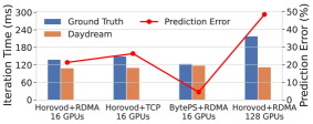
Figure 1: Training ResNet50 in 100Gbps network, batch size 32 per GPU (see Sec. 7.1 for testbed details)

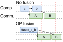
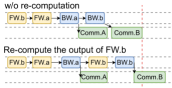
Figure 2: (a) Effect of op fusion: Comp. - computation op, Comm. - gradient synchronization; A/B is the gradient produced by op a/b; c is op fused from a and b. (b) Effect of re-computation: FW - forward propagation; BW - backward propagation; re-computation inserts a $FW.b$ before $BW.b$ since the output of the first $FW.b$ is not cached.

$\bullet$ Interactions/conflicts among different optimizations’ effects. For example, DL compilers such as XLA TensorFlow (2021) adopt op fusion to reduce GPU memory access and may fuse all back-propagation ops (i.e., as with the XLA auto-clustering algorithm), which delays communication of tensors produced by these ops. As shown in Fig. 2, although the computation time of the fused op becomes shorter, end-to-end training time increases due to less overlapping between computation and communication. Memory optimizations also interact with computation and communication. Fig. 2 shows that re-computation of intermediate results sacrifices training speed to reduce memory footprint. It may also delay tensor communication.

$\bullet$ Very large combined strategy space. The global DFG in distributed training of a DNN model is large, making it time-consuming to find the optimal set of strategies.

We design a search-based automatic optimizer framework, that effectively explores trade-offs among multiple optimizations to identify proper strategies for training acceleration.

3 Overview

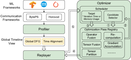
Figure 3: dPRO architecture.

dPRO includes three modules, as shown in Fig. 3.

Profiler  is a cross-framework distributed profiler, supporting three representative ML frameworks (TensorFlow, PyTorch and MXNet) and two parameter synchronization schemes (AllReduce and PS). The profiler collects time stamps (namely gTrace) of both computation ops and fine-grained communication ops. It also tracks dependencies among fine-grained communication ops and constructs the global data flow graph (global DFG). Our profiler uses op-level traces for computation ops, achieving similar high simulation accuracy as in Daydream (which uses kernel-level traces).

Replayer  simulates distributed training of a DNN model and estimates per-iteration training time of the global DFG.

Optimizer  takes as input a given DNN model and resource configurations (i.e., GPUs and their inter-connections), evaluates training performance of various strategy combinations using the replayer, and produces the best set of strategies found. We also provide an interface for developers to register custom optimization strategies.

We detail our design of key modules in next sections.

4 Profiler and Replayer

4.1 Global DFG Construction

The profiler automatically constructs a global DFG of the distributed training job, in which vertexes are computation and fine-grained communication ops and edges denote their dependencies. As shown in Fig. 4, the global DFG consists of local data flow graphs and communication topologies.

Local DFGs.  Most DL frameworks have the conception of data flow graphs for individual workers Abadi et al. (2016); Paszke et al. (2019); Chen et al. (2015). Our profiler extracts dependency information from each framework’s built-in graph definition and constructs a data flow graph for each worker accordingly. We further insert a pair of In/Out virtual ops for each tensor into each local DFG, indicating where the tensor transmission occurs.

Fine-grained Communication Topology  describes how each tensor is transferred between two devices, which contains two types of vertices (communication ops): (1) producer, which sends a tensor (partition) to another device; (2) consumer, which receives a tensor (partition) from another device. The profiler labels every transmission of a tensor (partition) between two devices with a unique transaction ID. A Middleman connects producers to the corresponding consumers that share the same transaction IDs. The communication topology for each tensor also contains a pair of In/Out virtual ops labeled with the tensor name, indicating the start/end of tensor transmission.

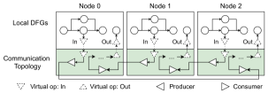
Figure 4: An illustration of the global DFG.

We connect local DFGs with the communication topology through In/Out virtual ops, and the global DFG is hence constructed. Decoupling global DFG construction into local DFGs and communication topology, we enable dPRO to support various ML frameworks and communication architectures. In a PS architecture, each PUSH (PULL) is regarded as a pair of SEND and RECV ops at a worker (PS) and a PS (worker), respectively. The unique transaction ID of each transmission can be produced using sender/receiver IPs, tensor name and whether it is PUSH or PULL. For AllReduce, we use a pair of SEND and RECV ops to represent the transmission of a chunk of the tensor to the next hop (e.g., along the ring in ring AllReduce). The transaction ID generation further uses chunk id of tensor partition and step id as in ring AllReduce Baidu (2017).

4.2 Trace Time Alignment

To combine traces collected on disparate workers/PSs and produce correct global DFG, one major obstacle is the time shift among machines where workers run. Not relying on accurate clock synchronization among machines, our profiler corrects the start time of RECV ops and obtains a more accurate communication duration of each tensor.

Let $\mathbf{W}$ and $\mathbf{P}$ denote the set of workers and PSs in a training job, respectively. For AllReduce, $\mathbf{P}$ is empty. Let $\bar{T}^{i}_{op}[st]$ and $\bar{T}^{i}_{op}[ed]$ be an op’s measured start and end timestamps on node $i\in\mathbf{P}\cup\mathbf{W}$, and $T^{i}_{op}[st]$ and $T^{i}_{op}[st]$ represent the respective adjusted time. Let node $0$ be a reference for other nodes to align their time to. We compute a time offset/drift of node $i$, $\theta_{i}$, as the difference in measured time between node $i$ and node $0$, i.e., ${T}^{0}_{op}=\bar{T}^{0}_{op}$ and ${T}^{i}_{op}=\theta_{i}+\bar{T}^{i}_{op}$. We leverage two observations for time alignment.

First, RECV ops on the same node receiving (even partitions of) the same tensor from the same sender in different training iterations, denoted as a RECV op family $f_{recv}$, should have similar execution time. Consider a pair of SEND and RECV from node $i$ to node $j$. Because RECV never happens before SEND, RECV’s true start time, $T_{recv}^{j}[st]+\theta_{j}$, should be clipped by the start time of SEND, $T_{send}^{i}[st]+\theta_{i}$, which changes the communication time from $(T_{recv}^{j}[ed]+\theta_{j})-(T_{recv}^{j}[st]+\theta_{j})$ to $T_{recv}^{j}[ed]+\theta_{j}-max(T_{recv}^{j}[st]+\theta_{j},T_{send}^{i}[st]+\theta_{i})$. With time adjustment, we should minimize the variance of execution time of RECV ops in the same RECV op family:

$$O_{1}=\sum_{f_{recv}\in\mathcal{F}_{recv}}Var_{recv_{j}\in f_{recv}}\left(T_{recv}^{j}[ed]\right.$$

$$\left.+\theta_{j}-max(T_{recv}^{j}[st]+\theta_{j},T_{send}^{i}[st]+\theta_{i})\right)$$

where $\mathcal{F}_{recv}$ is the set of all RECV op families and $i$ denotes the node where the sender of the tensor of $f_{recv}$ resides.

Second, nodes on the same physical machine should have the same time offset because they share the same physical clock. Let $\mathcal{M}$ be the set of all physical machines and $g_{m}$ be the set of nodes on machine $m$. We should ensure the time offset of workers on the same machine as close as possible:

$$O_{2}=\sum_{m\in\mathcal{M}}Var_{i\in g_{m}}(\theta_{i})$$

We compute time offsets $\theta_{i}$’s for time alignment among distributed nodes, by solving the following optimization:

$$\min_{\theta_{i}:i\in\mathbf{P}\cup\mathbf{W}}a_{1}O_{1}+a_{2}O2$$

$$~{}~{}\textrm{s.t.}\quad\theta_{0}=0,$$

$$~{}~{}~{}~{}~{}~{}~{}~{}~{}~{}\theta_{i}-\theta_{j}\leq\bar{T}^{j}_{o_{2}}-\bar{T}^{i}_{o_{1}},$$

$$~{}~{}~{}~{}~{}~{}\forall(i,j)\in(\mathbf{W}\times\mathbf{P})\cup(\mathbf{P}\times\mathbf{W}),i\neq j,(o_{1},o_{2})\in\mathrm{E}$$

Here $a_{1}\geq 0$ and $a_{2}\geq 0$ are two coefficients gauging the weights of the two objectives, and $E$ is the set of inter-op dependencies. The constraints ensure inter-op dependencies for time alignment, i.e., the adjusted time of an op $o_{2}$ on $j$ ($\bar{T}_{o_{2}}^{j}+\theta_{j}$) that depends on op $o_{1}$ on $i$, is not earlier than the adjusted time of $o_{1}$ ($\bar{T}_{o_{1}}^{i}+\theta_{i}$). The optimization problem can be solved in a few seconds using the state-of-the-art optimization libraries CVXPY (2020).

4.3 Replayer

The replayer simulates the execution of the global DFG based on a modified Kahn’s algorithm Kahn (1962) of topological sorting. Instead of using a global ready queue (used in Daydream or Kahn’s algorithm), for a distributed training job, we regard each worker/PS and each communication link as one device, and the replayer maintains a queue and a device time (end time of the last op executed on the device) for each device. An op is enqueued to the queue of corresponding device once it is ready, i.e., all its predecessor ops are executed. The replayer iteratively picks the device with the smallest device time, dequeues an op from the head of this queue and updates the corresponding device time with the op’s execution time. After all ops in the global DFG are run, we take the largest device time as the iteration time. Although there might be multiple feasible topological sortings, dPRO’s replayer can generate the most likely one by averaging op execution time over 10 training iterations and imitating the FIFO queue in ML framework’s engines.

The replayer also produces an execution graph by adding additional edges into the global DFG, indicating execution ordering between ops running in the same device, and computes the critical path on the execution graph, for bottleneck identification by the optimizer.

5 Optimizer

Given a global DFG $\mathcal{G}$ of a distributed DNN training job and a set of optimization strategies $\mathcal{S}$, the optimizer identifies the bottlenecks in the global graph through training replay and produces a subset of optimization strategies, $\mathcal{S}^{*}\in\mathcal{S}$, minimizing per-iteration training time (referred to as the iteration time):

$$min_{\mathcal{S}^{\prime}\in\mathcal{S}}\textsc{IterationTime}(f(\mathcal{G},\mathcal{S}^{\prime}))$$

where $\mathcal{G}^{\prime}=f(\mathcal{G},\mathcal{S}^{\prime})$ is the modified global DFG after applying strategies in $\mathcal{S}^{\prime}$ to the original global DFG $\mathcal{G}$.

5.1 Theory Foundation

The main idea of our optimizer is to iteratively check and optimize the critical path of the global execution graph. The critical path $C$ contains a sequence of computation and communication ops: $C=[p_{0},p_{1},...,p_{i},q_{i},q_{i+1},...,q_{|C|-1}]$, where $p_{0},p_{1},...,p_{i}$ are computation ops and $q_{i},q_{1},...,q_{|C|-1}$ are communication ops. Here, we group fine-grained communication ops in the global DFG for the transmission of tensor $n$ (e.g., SEND and RECV) as one communication op $q_{n}$. Fig. 5 depicts an example of the critical path and the correspondence between each pair of $p_{n}/q_{n},n=0,1,...|C|-1$. Since gradient tensors are dependent on computation ops, the critical path always starts from a sequence of computation ops and ends with a sequence of communication ops.

Note that each computation op $p_{n},n=1,\ldots,i$ on the critical path may correspond to a communication op $q_{n}$ (each backward computation op has a corresponding tensor communication op, while we treat $q_{n}$ for a forward computation op $p_{n}$ as null); the corresponding communication ops do not lie on the critical path before $p_{i}$, because computation ops are the bottleneck in this phase; On the other hand, each communication op $q_{n},n=i,\ldots,|C|-1$ on the critical path corresponds to a computation op $p_{n}$ which may not lie on the critical path.

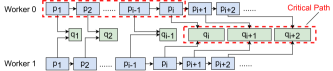
Figure 5: Illustration of Critical Path.

The optimizer inspects the critical path form $p_{0}$ to $q_{|C|-1}$. For each op, $p_{n},n=1,\ldots,i$ or $q_{n},n=i,\ldots,|C|-1$, a decision $d_{n}$ is made on whether op fusion and/or tensor fusion should be applied: 1) $d_{n}=opfs$, fusing two computation ops $p_{n-1}$ and $p_{n}$; 2) $d_{n}=tsfs$, fusing the two tensors $q_{n-1}$ and $q_{n}$ (those corresponding to computation ops $p_{n-1}$ and $p_{n}$); 3) $d_{n}=opfs\_tsfs$, fusing $p_{n-1}$ and $p_{n}$ and fusing tensors $q_{n-1}$ and $q_{n}$; 4) $d_{n}=null$, no fusion. We have $d_{0}=null$. When tensor partition is enabled, the optimizer also decides an optimal partition number $k_{n}$ for the tensor of op $p_{n}$ or $q_{n}$ on the critical path. Unlike op and tensor fusion, tensor partition does not hurt computation-communication overlapping, but only affects tensor synchronization time, which inspires us to adopt the optimal partition size for each possible choice of $d_{n}$, before comparing their performance.

Let $T_{n}$ denote the duration from the start of the global DFG execution till the completion of computation op $p_{n}$ and corresponding communication op $p_{n}$, i.e., $T_{n}=\max(p_{n}^{e},q_{n}^{e})$ (see Table 1 for notation definitions). The optimizer finds optimal decisions $\mathcal{D}=[d_{0},d_{1},...,d_{|C|-1}],$ and $\mathcal{K}=[k_{0},k_{1},...,k_{|C|-1}]$ that minimize the duration of the critical path: $\min_{\mathcal{D},\mathcal{K}}T_{|C|-1}$.

Table 1: Notation

Symbol	Description	Calculation
$p_{n}^{d}$	execution time of computation op $p_{n}$	profiled
$p_{n}^{e}$	end time of computation op $p_{n}$	decided during the search process
$q_{n}^{d}$	execution time of synchronizing tensor $q_{n}$	estimated using partial replay
$q_{n}^{s}$	size of tensor $q_{n}$	profiled
$q_{n}^{e}$	end time of communication op $q_{n}$	decided during the search process
$d_{n}$	strategy taken on the $n$-th op in the critical path	decided during the search process
$k_{n}$	partition number of tensor $q_{n}$	computed during the search process

We analyze conditions for applying the optimization techniques, deriving insights to tailor a strategy search algorithm. Let $opfs\_time(p_{n-1},p_{n})$ be the execution time of the fused op after fusing $p_{n-1}$ and $p_{n}$.

Theorem 1 (Op Fusion)

If $q_{n-1}^{d}\leq p_{n}^{d}+p_{n-1}^{d}-opfs\_time(p_{n-1},p_{n})$, $T_{n}$ achieved with this op fusion is smaller than no fusion, i.e., $T_{n}(d_{n}=opfs)\leq T_{n}(d_{n}=null)$ (fusing $p_{n-1}$ and $p_{n}$ is better than not); otherwise, $T_{n}(d_{n}=opfs)\geq T_{n}(d_{n}=null)$, i.e., fusing $p_{n-1}$ and $p_{n}$ leads to a worse performance.

Let $t_{sync}(s,k)$ be the time to synchronize a tensor of size $s$, divided to $k$ partitions, i.e., execution time of the complete synchronization operation on this tensor (using either PS or AllReduce). Given a tensor of size $s$, we use $k^{*}[s]$ to denote the optimal partition number that minimizes $t_{sync}$.

Theorem 2 (Tensor Fusion/Partition)

If $q_{n-1}^{e}>p_{n}^{e}+t_{sync}(q_{n-1}^{s}+q_{n}^{s},k^{*}[q_{n-1}^{s}+q_{n}^{s}])-t_{sync}(q_{n}^{s},k^{*}[q_{n}^{s}])$, then $T_{n}$ achieved by fusing tensors $q_{n-1}$ and $q_{n}$ is smaller than no fusion, i.e., $T_{n}(d_{n}=tsfs,k_{n}=k^{*}[q_{n-1}^{s}+q_{n}^{s}])<T_{n}(d_{n}=null,k_{n}=k^{*}[q_{n}^{s}])$ (fusing $q_{n-1}$ and $q_{n}$ is better than not); otherwise, $q_{n-1}$ and $q_{n}$ should not be fused.

When considering op fusion and tensor fusion/partition together, if fusing two computation (communication) ops is better than not, their corresponding communication (computation) ops - if there are - should also be fused, without sacrificing computation-communication overlapping.

Theorem 3 (Op Fusion and Tensor Fusion/Partition)

$T_{n}(d_{n}=opfs\_tsfs,k_{n}=k^{*}[q_{n-1}^{s}+q_{n}^{s}])\leq T_{n}(d_{n}=tsfs,k_{n}=k^{*}[q_{n-1}^{s}+q_{n}^{s}])$ and $T_{n}(d_{n}=opfs\_tsfs,k_{n}=k^{*}[q_{n-1}^{s}+q_{n}^{s}])\leq T_{n}(d_{n}=opfs,k_{n}^{*}[q_{n}^{s}])$.

See the appendix hu2 (2022) for proofs of Theorems 1, 2 and 3.

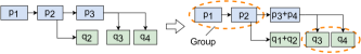
Figure 6: Illustration of Coarsened View, where $p_{1}$ has no learnable parameter but $p_{3}$ has two.

5.2 Diagnosis and Optimization Algorithm

An ablation of dPRO’s optimizer module is given in Fig. 3. The optimizer maintains a Graph Pass Registry including various optimization techniques. Each Graph Pass in the Registry corresponds to an optimization technique, such as op fusion, tensor fusion, tensor partition, etc.

The optimizer analyzes the bottlenecks in the global DFG and optimizes them in an iterative manner. The optimizer algorithm is given in Alg. 1. At the beginning, the optimizer evaluates the iteration time and memory usage of the original global DFG $\mathcal{G}$ by replaying it with the replayer. If the memory usage exceeds the memory budget (specified by the user), the memory-optimization passes are invoked to reduce the memory footprint (see the appendix hu2 (2022) for details).

Then the optimizer proceeds with throughput optimization, that minimizes the makespan of the critical path in the global execution graph. Given a critical path $C=[p_{0},p_{1},...,p_{i},q_{i},q_{i+1},...,q_{|C|-1}]$, the optimizer first examines the computation ops $p_{n},n=1,\ldots,i$ in order. Because the performance of this segment of the critical path is computation-bound, the optimizer first evaluates whether op fusion should be applied on $p_{n-1}$ and $p_{n}$ according to Theorem 1. If so, it invokes the op fusion pass to fuse $p_{n-1}$ and $p_{n}$, as well as the tensor fusion pass to fuse the corresponding two tensors $q_{n-1}$ and $q_{n}$ (Theorem 3). An optimal partition number $k^{*}$ is then computed and applied (if $k^{*}>1$) on the fused or non-fused tensor $q_{n}$.

Next, the optimizer inspects the communication ops $q_{n},n=i,\ldots,|C|-1$, on the critical path. In this segment, the performance is communication-bound. The optimizer first computes the optimal partition number $k^{*}$ on the fused and non-fused tensor $q_{n}$ and checks whether tensor fusion should be applied to $q_{n-1}$ and $q_{n}$ according to Theorem 2. If so, the optimizer invokes the tensor fusion pass to fuses $q_{n-1}$ and $q_{n}$, as well as the corresponding computation ops $p_{n-1}$ and $p_{n}$ (Theorem 3). Then the optimal partition number $k^{*}$ on fused or non-fused tensor is applied accordingly.

After applying the optimizations, the global DFG $G$ is updated. The optimizer uses the replayer to update the critical path $C$ and then repeats the search on the new critical path.

The fused op execution time, $opfs\_time(p_{n-1},p_{n})$, can be obtained by profiling the fused op in an offline manner (as we will do in the experiments) or use a cost model Kaufman et al. (2019). The time to synchronize a tensor, $t_{sync}(s,k)$, is estimated with partial replay of the subgraph including all relevant communication ops (Sec. 5.3). The optimal partition number of a tensor is obtained through grid search.

Algorithm 1 Diagnosis and Optimization Algorithm

1:  If OOM, invoke the Memory Optimization Pass

2:  Construct the Coarsened View  and fuse ops/tensors in the same group.

3:  The replayer computes an initial critical path $C=[p_{0},p_{1},...,p_{i},q_{i},q_{i+1},...,q_{|C|-1}]$

4:  while search time budget not exhausted and speed-up not converged do

5:     for $n=0\rightarrow i$ do

6:        if $q_{n-1}^{d}<p_{n}^{d}+p_{n-1}^{d}-opfs\_time(p_{n-1},p_{n})$ then

7:           OPFusion($p_{n-1}$, $p_{n}$) [Theorem 1]

8:           TensorFusion($q_{n-1}$ , $q_{n}$) [Theorem 3]

9:           $k^{*}\leftarrow\textsc{OptPartNum}(q_{n-1}+q_{n})$

10:           Partition fused tensor $q_{n-1}^{s}+q_{n}^{s}$ evenly by $k^{*}$

11:        else

12:           // tensor partition only

13:           $k^{*}\leftarrow\textsc{OptPartNum}(q_{n})$

14:           Partition tensor $q_{n}^{s}$ evenly by $k^{*}$

15:        end if

16:     end for

17:     for $n=i\rightarrow|C|-1$ do

18:        if $q_{n-1}^{e}>p_{n}^{e}+t_{sync}(q_{n-1}^{s}+q_{n}^{s},k^{*}[q_{n-1}^{s}+q_{n}^{s}])-t_{sync}(q_{n}^{s},k^{*}[q_{n}^{s}])$ then

19:           TensorFusion( $q_{n-1}$, $q_{n}$) [Theorem 2]

20:           OPFusion( $p_{n-1}$ , $p_{n}$) [Theorem 3]

21:           Partition fused tensor $q_{n-1}+q_{n}$ evenly by $k^{*}=\textsc{OptPartNum}(q_{n-1}+q_{n})$

22:        else

23:           Partition tensor $q_{n}^{s}$ evenly by $k^{*}=\textsc{OptPartNum}(q_{n})$

24:        end if

25:     end for

26:     Execute the updated global DFG using the replayer and obtain a new critical path $C=[p_{0},p_{1},...,p_{i},q_{i},q_{i+1},...,q_{|C|-1}]$

27:  end while

5.3 Search Speed-up

It is time-consuming to exhaustively explore the large strategy space, e.g., it takes more than 24 hours to search for the optimal optimization strategies for BERT Base. We propose several techniques to expedite the search process.

Coarsened View. Inspired by Theorem 3, we coarsen the global DFG during the search process, namely constructing the Coarsened View: we put computation ops that do not produce tensors but are close to one tensor-producing computation op into one group (together with the latter), and communication ops connected to the same computation op into one group. Ops or tensors in the same group are fused, and we search for optimization strategies based on such a coarsened view of the global DFG (line 1 of Alg. 1). Fig. 6 gives an illustration. $p_{1}$ produces no tensor ($q_{1}=null$) and is connected to $p_{2}$ which generates a tensor $q_{2}$; $p_{1}$ and $p_{2}$ are fused into one group. The rationale lies in that: we can view tensor $q_{2}$ as a fusion of $q_{1}=null$ and $q_{2}$; then according to Theorem 3, fusing $p_{1}$ and $p_{2}$ leads to a better performance. $q_{3}$ and $q_{4}$ are both tensors produced by $p_{3}$ (e.g., the BatchNorm Layer has two learnable parameters Ioffe & Szegedy (2015)), and they are put into one group. This is because we can regard $p_{3}$ as a fusion of $p_{3}$ and $p_{4}=null$; then fusing $q_{3}$ and $q_{4}$ is better than not based on Theorem 3. We construct Coarsened View using a backtracking algorithm detailed in the appendix hu2 (2022).

Partial Replay. To avoid frequently replaying the entire global DFG during strategy search (for estimating $t_{sync}(s,k)$), the replayer supports partial simulation. Given the current global DFG $G$, the replayer identifies all communication ops $\mathcal{S}_{p}$ related to the tensor, and generates a subgraph $G^{\prime}$, which contains the ops in $\mathcal{S}_{p}$ and the edges between those ops. Execution of the subgraph is simulated to produce the tensor synchronization time.

Exploiting Symmetry. We further leverage the symmetry in the global DFG of state-of-the-art DNNs to accelerate strategy search. For example, BERT Devlin et al. (2019) includes multiple transformer blocks; the strategies applied inside one block can be used in other blocks as well. For data parallel training with homogeneous workers, the optimizations applied on one critical path can actually be applied to multiple workers.

6 Implementation

Profiler.  To profile computation ops, we use the native profiler of each ML framework with minor modifications.

$\bullet$ TensorFlow. We implemented dPRO with TensorFlow 2.4 in the graph execution mode. We modify tf.profiler to collect computation traces with absolute time and extract dependencies from tf.RunMetadata.partition_graphs.

$\bullet$ MXNet. We collect computation traces using $mxnet.profiler$, with some modifications to ensure a unique trace name for each op. We extract op dependencies through $mxnet.Symbol.debug\_str()$ API.

$\bullet$ Communication. We use Horovod Sergeev & Del Balso (2018) as the AllReduce communication library, which uses NCCL NVIDIA (2021c) for collective communication across GPUs. We dive into NCCL (adding 318 LoCs) to collect timestamps of SEND/RECV of the tensor chunks. We adopt BytePS Jiang et al. (2020) for PS-based communication and add around 400 LoCs to its communication library, ps-lite Li et al. (2014), for recording timestamps of PUSH and PULL of each tensor.

Replayer.  We implement it using Python with 3653 LoCs.

Optimizer.  We implement the optimizer and all optimization passes in Python with 5745 LoCs. We implement op fusion on TensorFlow using XLA TensorFlow (2021), and modify it to allow manual control of which ops to be fused in detail, in order to apply our identified strategies. We modify Horovod and BytePS to enable customized tensor fusion pattern and tensor partition size.

APIs and Commands.  dPRO provides a simple programming interface for trace collection. The following shows the APIs for trace collection on TensorFlow, with only 2 additional LoCs: a recorder is defined, with which the wrapper decides when to start/finish profiling and output traces.

⬇

recorder = dpro.Recorder(model)

@dpro.profile(recorder)

def train_one_step():

# define one training step here

After profiling, a user can call the commands as follows to invoke the profiler, replayer and optimizer, respectively.

⬇

$ dpro profile <python program> -o <trace path>

$ dpro replay <trace path>

$ dpro optimize <trace path>

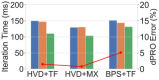
(a) ResNet50, TCP

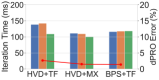
(b) ResNet50, RDMA

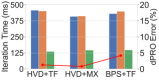
(c) VGG16, TCP

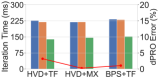
(d) VGG16, RDMA

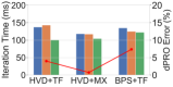
(e) InceptionV3, TCP

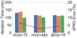
(f) InceptionV3, RDMA

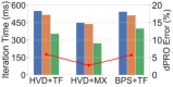
(g) BERT Base, TCP

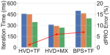
(h) BERT Base, RDMA

Figure 7: Replay Accuracy: dPRO replayer vs. Daydream simulator

7 Evaluation

7.1 Experiment Setup

Testbed. We evaluate dPRO in a production ML cluster and use up to 128 Tesla V100 32GB GPUs (on 16 servers). The GPU servers are equipped with NVLinks and inter-connected with 100Gbps bandwidth using Mellanox CX-5 single-port NICs. We use CUDA v10.2 NVIDIA (2020) and cuDNN v7.6.5 NVIDIA (2021b) in our experiments. In our default, we use 16 GPUs (on 2 servers).

Benchmarks. We train 4 DNN models: BERT Base Devlin et al. (2019) for natural language processing, and ResNet50 He et al. (2016), VGG16 Simonyan & Zisserman (2015) and InceptionV3 Szegedy et al. (2016) for image classification. Each model is trained using various combinations of ML framework, communication library and inter-server connectivity: Horovod TensorFlow (HVD+TF), BytePS TensorFlow (BPS+TF), Horovod MXNet (HVD+MX), BytePS MXNet (BPS+MX), each with TCP or RDMA inter-connectivity.

Baselines. We compare dPRO with the state of the art in various aspects: 1) Daydream for replay accuracy: Daydream Zhu et al. (2020) estimates the iteration time of distributed training using a local DFG and inserts one coarse-grained communication op for each tensor, whose communication time is calculated by $tensor\mbox{ }size/bandwidth$. 2) XLA’s default op fusion, which fuses as many computation ops as possible. 3) Horovod’s default tensor fusion, which fuses tensors in intervals of 5ms with fused tensor size upper-bounded by 64MB, as well as 4) Horovod Autotune, which automatically tunes the interval and upper bound. 5) BytePS’s default setting, in which tensors are partitioned with a partition size of 4MB.

By default, the batch size is 32 per GPU. Iteration time is averaged over 10 training steps after the warm-up phase. More experimental results can be found in the appendix hu2 (2022).

7.2 Replay Accuracy

Fig. 7 compares the predicted iteration time by dPRO and Daydream’s simulator against the real time measured in actual training. dPRO’s replay error is less than $5\%$ in most cases, while Daydream’s error rate is up to $70.2\%$.

Table 2: Deep Dive of Simulation Error Comparison for TensorFlow Horovod RDMA

Model	Experiment	Time (ms)
		Iteration	FW	BW
ResNet50	Ground truth	138.64	34.78	71.34
	dPRO	142.31	34.20	70.32
	Daydream	109.19	34.69	70.04
BERT Base	Ground truth	459.62	107.49	185.66
	dPRO	453.83	106.58	187.05
	Daydream	345.68	106.80	185.79

Table 2 shows detailed estimated durations of forward and backward propagation. We observe that both dPRO and Daydream predict forward and backward execution time accurately, so the error mainly arises from the estimation of communication time. Daydream’s simple approach for communication time prediction does not capture effects of message queuing, network and communication protocols, resulting in larger errors in training simulation.

We also note that the overhead introduced by dPRO ($5.86\%$ in our experiments) is almost the same as that of ML frameworks’ built-in profilers, indicating that our detailed communication profiling introduces little extra overhead.

7.3 Trace Time Alignment

To evaluate the effect of our trace time alignment, we collect traces by running distributed training jobs on different clusters, where NTP is enabled. Fig. 8 shows errors of iteration time estimated by our replayer (as compared to ground truth) with and without time alignment. Although workers have been synchronized with NTP or with no clock drift (as in the 8-GPU jobs), inaccuracy of communication traces (e.g., due to RECV op) still leads to large replay errors (up to $36.7\%$), while errors are reduced to $<5\%$ with time alignment. Since larger clusters are more likely to experience large clock drifts and queuing delay, the simulation error gap between dPRO w/ and w/o trace time alignment becomes significantly larger as the cluster size grows.

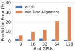
(a) VGG16, HVD RDMA

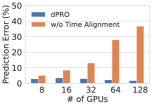
(b) BERT Base, HVD RDMA

Figure 8: Effects of trace timeline alignment. Workers in the 8-GPU jobs are located on the same physical machine.

7.4 Optimizer Performance

Computation op fusion.  We first evaluate the performance of op fusion strategies found by the optimizer, temporarily excluding other optimization techniques from the search space. Fig. 9 shows the actual training throughput when applying the respective strategies in real distributed training. dPRO’s op fusion ($dPRO{}\_OPFS$) yields up to $51.843\%$ speed-up as compared to XLA’s default strategies. Although XLA is widely used to accelerate training on a single machine, the results show that in distributed training, simply fusing many ops as with XLA may even slow down the training progress, due mainly to reduced overlap between computation and communication.

Tensor Fusion and Tensor Partition.  We next evaluate the effect of tensor fusion strategies found by dPRO’s optimizer ($dPRO{}\_TSFS$). Note that both tensor fusion and tensor partition (BytePS’s default partition strategy) are enabled when we use BytePS as the communication library. As Fig. 9 shows, our strategies achieve up to $19.1\%$ speed-up compared with default Horovod and BytePS.

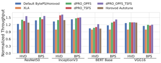
Figure 9: Performance of op fusion and tensor fusion: training different DNNs on TensorFlow

Interaction between op fusion and tensor fusion.  We further evaluate combined op fusion and tensor fusion/partition strategies identified by our optimizer ($dPRO{}\_OPFS\_TSFS$). In Fig. 9, We observe that our combined strategies perform the best in most cases: up to $62.95\%$ acceleration as compared to XLA and up to $26.44\%$ speed-up compared to default Horovod and BytePS.

Integrating memory optimization.  In this experiment, we evaluate the accuracy of peak memory estimation with our replayer. Table 3 shows the actual memory consumption and estimated peak memory with our replayer, when training different DNN models on TensorFlow with a batch size of 32 per GPU. The relative errors across different models are at most 5.25%.

Table 3: Memory estimation accuracy

Model	Real (GB)	Est. (GB)	Relative Error (%)
BERT Base	9.96	10.25	2.83
ResNet50	5.41	5.71	5.25
InceptionV3	3.91	4.05	3.46
VGG16	5.91	5.83	1.37

We further investigate the effects of memory optimization (gradient accumulation and re-computation to reduce memory footprint) performed at the start of our search algorithm. Especially, the algorithm evaluates iteration time and memory incurred by the two memory optimizations and selects the one achieving the shorter time under the memory budget. Table 4 presents the results when training BERT Base using a batch size of 64 per GPU, on 16GB V100 GPUs (an OOM error occurs without memory optimization). Re-computation performs better than gradient accumulation in both time and memory consumption in this setting. Moreover, prediction results with our replayer match well the measured data collected in actual training.

Table 4: Iteration time and memory usage: BERT Base (TensorFlow Horovod RDMA) on 16 GPUs with batch size 64 per GPU.

Optimization Method	Time (ms)		Memory (GB)
	Real	Est.	Real	Est.
w/o optimization	622.12	613.87	16.42	16.97
Re-computation	696.13	672.60	7.43	7.20
Gradient Accumulation	714.22	708.57	9.96	10.25

Table 5: Time to search optimal op fusion and tensor fusion/partition strategies on TensorFlow BytePS (in hours).

Model	Straw- man	+Coarsened View	+Partial Replay	+Sym- metry
ResNet50	14.60	5.35	0.91	0.29
VGG16	11.97	3.74	0.71	0.04
InceptionV3	16.75	6.13	1.04	0.47
BERT Base	$>$24	22.01	3.25	0.49

Search speedup.  We evaluate the effects of our techniques used to accelerate the strategy search process. Table 5 gives the algorithm running time, where the search ends when the per-iteration training time evaluated with the identified strategies changes little over 5 search iterations. The strawman case is Alg. 1 without any search speed-up methods, which costs tens of hours. The last three columns show the search time when the respective speed-up method is in place (in addition to the previous one(s)). With more speed-up methods applied, the strategy search time decreases significantly and we can finish the search within a short time. Note that all experimental results we presented earlier are based on strategies found with the speeded-up search.

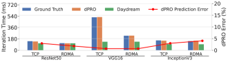
(a) Replay Accuracy Comparison

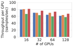
(b) VGG16

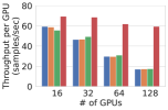
(c) BERT Base

Figure 10: Performance when training DNN models using up to 128 V100 GPUs on TensorFlow + Horovod

7.5 Large-Scale Distributed Training

We further evaluate dPRO on replaying and optimizing distributed DNN training using large-scale clusters. In Fig. 10, we observe the following: (1) as the cluster size grows, DNN training becomes slower since the communication overhead is larger for synchronizing among more GPUs. (2) Our replayer can still simulate such distributed training accurately, with an error lower than $5\%$ in most cases (up to $5.6\%$); Daydream’s prediction error increases substantially (up to $73.8\%$) as the cluster size grows. (3) dPRO’s combined strategies reach the best scalability and yield up to $3.48\times$ speed-up compared to XLA’s default strategies.

8 Conclusion

dPRO is a diagnosis and optimizing toolkit for distributed DNN training. It can simulate distributed training with low error under different configurations and efficiently explore collaborative effects among multiple DNN optimizations. The key design points include: 1) building an accurate global DFG by collecting fine-grained traces and aligning timestamps in different devices; 2) designing an optimization framework to search for combined optimization strategies efficiently.

dPRO, along with the time alignment method, can also be applied to model or pipeline-parallel training, where each local DFG only contains part of ops in the DNN model and the communication topology models transmission of activations between workers. We also provide an interface for developers to register custom optimization strategies (e.g., mixed precision), and the optimizer can automatically explore all registered optimizations (see the appendix hu2 (2022) for more details).

9 Acknowledgement

This work was supported by Hong Kong Innovation and Technology Commission’s Innovation and Technology Fund (Partnership Research Programme with ByteDance Limited, Award No. PRP/082/20FX), and grants from Hong Kong RGC under the contracts HKU 17204619, 17208920 and 17207621.

References

- hor (2020) Horovod Tensor Fusion, 2020. https://horovod.readthedocs.io/en/stable/tensor-fusion_include.html.
- nvi (2020) Training With Mixed Precision, 2020. https://docs.nvidia.com/deeplearning/performance/mixed-precision-training/index.html.
- ten (2020) TensorFlow Operation Fusion, 2020. https://www.tensorflow.org/lite/convert/operation_fusion.
- hu2 (2022) dPRO FigShare Software, 2022. https://doi.org/10.6084/m9.figshare.19165622.v3.
- Abadi et al. (2016) Abadi, M., Barham, P., Chen, J., Chen, Z., Davis, A., Dean, J., Devin, M., Ghemawat, S., Irving, G., Isard, M., et al. Tensorflow: A System for Large-scale Machine Learning. In Proceedings of the 12th USENIX Symposium on Operating Systems Design and Implementation, 2016.
- Alistarh et al. (2017) Alistarh, D., Grubic, D., Li, J., Tomioka, R., and Vojnovic, M. QSGD: Communication-Efficient SGD via Gradient Quantization and Encoding. In Proceedings of Advances in Neural Information Processing Systems, 2017.
- Baidu (2017) Baidu. Ring AllReduce, 2017. https://github.com/baidu-research/baidu-allreduce.
- Bao et al. (2020) Bao, Y., Peng, Y., Chen, Y., and Wu, C. Preemptive All-reduce Scheduling for Expediting Distributed DNN Training. In Proceedings of IEEE International Conference on Computer Communications, 2020.
- Bernstein et al. (2018) Bernstein, J., Wang, Y.-X., Azizzadenesheli, K., and Anandkumar, A. SignSGD: Compressed Optimisation for Non-Convex Problems. In Proceedings of International Conference on Machine Learning, 2018.
- ByteDance (2020) ByteDance. BytePS Timeline, 2020. https://github.com/bytedance/byteps/blob/master/docs/timeline.md.
- Chen et al. (2015) Chen, T., Li, M., Li, Y., Lin, M., Wang, N., Wang, M., Xiao, T., Xu, B., Zhang, C., and Zhang, Z. MXNet: A Flexible and Efficient Machine Learning Library for Heterogeneous Distributed Systems. arXiv preprint arXiv:1512.01274, 2015.
- Chen et al. (2016) Chen, T., Xu, B., Zhang, C., and Guestrin, C. Training Deep Nets with Sublinear Memory Cost. arXiv preprint arXiv:1604.06174, 2016.
- Chen et al. (2020) Chen, Y., Peng, Y., Bao, Y., Wu, C., Zhu, Y., and Guo, C. Elastic Parameter Server Load Distribution in Deep Learning Clusters. In Proceedings of the 11th ACM Symposium on Cloud Computing, 2020.
- Cho et al. (2019) Cho, M., Finkler, U., Serrano, M., Kung, D., and Hunter, H. BlueConnect: Decomposing All-reduce for Deep Learning on Heterogeneous Network Hierarchy. IBM Journal of Research and Development, 2019.
- Curtsinger & Berger (2015) Curtsinger, C. and Berger, E. D. Coz: Finding Code that Counts with Causal Profiling. In Proceedings of the 25th Symposium on Operating Systems Principles, 2015.
- CVXPY (2020) CVXPY. CVXPY, 2020. https://www.cvxpy.org/tutorial/advanced/index.html.
- Devlin et al. (2019) Devlin, J., Chang, M.-W., Lee, K., and Toutanova, K. BERT: Pre-training of Deep Bidirectional Transformers for Language Understanding. In Proceedings of the North American Chapter of the Association for Computational Linguistics: Human Language Technologies, 2019.
- Foundation (2019) Foundation, L. A. . D. Horovod, Analyze Performance, 2019. https://horovod.readthedocs.io/en/stable/timeline_include.html.
- Geng et al. (2018) Geng, Y., Liu, S., Yin, Z., Naik, A., Prabhakar, B., Rosenblum, M., and Vahdat, A. Exploiting a natural network effect for scalable, fine-grained clock synchronization. In Proceedings of 15th USENIX Symposium on Networked Systems Design and Implementation, 2018.
- He et al. (2016) He, K., Zhang, X., Ren, S., and Sun, J. Deep Residual Learning for Image Recognition. In Proceedings of the IEEE conference on Computer Vision and Pattern Recognition, 2016.
- Ho et al. (2013) Ho, Q., Cipar, J., Cui, H., Lee, S., Kim, J. K., Gibbons, P. B., Gibson, G. A., Ganger, G., and Xing, E. P. More Effective Distributed ML via a Stale Synchronous Parallel Parameter Server. Proceedings of Advances in Neural Information Processing Systems, 2013.
- Hu et al. (2020) Hu, H., Wang, D., and Wu, C. Distributed Machine Learning through Heterogeneous Edge Systems. In Proceedings of the AAAI Conference on Artificial Intelligence, 2020.
- Huang et al. (2019) Huang, Y., Cheng, Y., Bapna, A., Firat, O., Chen, D., Chen, M., Lee, H., Ngiam, J., Le, Q. V., Wu, Y., et al. Gpipe: Efficient Training of Giant Neural Networks using Pipeline Parallelism. In Proceedings of Advances in Neural Information Processing Systems, 2019.
- Ioffe & Szegedy (2015) Ioffe, S. and Szegedy, C. Batch normalization: Accelerating deep network training by reducing internal covariate shift. In Proceedings of International Conference on Machine Learning, 2015.
- Jayarajan et al. (2019) Jayarajan, A., Wei, J., Gibson, G., Fedorova, A., and Pekhimenko, G. Priority-based Parameter Propagation for Distributed DNN Training. In Proceedings of Machine Learning and Systems, 2019.
- Jia et al. (2019a) Jia, Z., Padon, O., Thomas, J., Warszawski, T., Zaharia, M., and Aiken, A. TASO: Optimizing Deep Learning Computation with Automatic Generation of Graph Substitutions. In Proceedings of the 27th ACM Symposium on Operating Systems Principles, 2019a.
- Jia et al. (2019b) Jia, Z., Thomas, J., Warszawski, T., Gao, M., Zaharia, M., and Aiken, A. Optimizing DNN Computation with Relaxed Graph Substitutions. In Proceedings of Machine Learning and Systems, 2019b.
- Jia et al. (2019c) Jia, Z., Zaharia, M., and Aiken, A. Beyond Data and Model Parallelism for Deep Neural Networks. In Proceedings of Machine Learning and Systems, 2019c.
- Jiang et al. (2020) Jiang, Y., Zhu, Y., Lan, C., Yi, B., Cui, Y., and Guo, C. A Unified Architecture for Accelerating Distributed DNN Training in Heterogeneous GPU/CPU Clusters. In Proceedings of the 14th USENIX Symposium on Operating Systems Design and Implementation, 2020.
- Kahn (1962) Kahn, A. B. Topological Sorting of Large Networks. Communications of the ACM, 1962.
- Kaufman et al. (2019) Kaufman, S., Phothilimtha, P., and Burrows, M. Learned TPU Cost Model for XLA Tensor Programs. In Proceedings of the Workshop on ML for Systems at NeurIPS 2019, 2019.
- Lepikhin et al. (2021) Lepikhin, D., Lee, H., Xu, Y., Chen, D., Firat, O., Huang, Y., Krikun, M., Shazeer, N., and Chen, Z. GShard: Scaling Giant Models with Conditional Computation and Automatic Sharding. In Proceedings of International Conference on Learning Representations, 2021.
- Li et al. (2014) Li, M., Andersen, D. G., Park, J. W., Smola, A. J., Ahmed, A., Josifovski, V., Long, J., Shekita, E. J., and Su, B.-Y. Scaling Distributed Machine Learning with the Parameter Server. In Proceedings of the 11th USENIX Symposium on Operating Systems Design and Implementation, 2014.
- Mai et al. (2020) Mai, L., Li, G., Wagenländer, M., Fertakis, K., Brabete, A.-O., and Pietzuch, P. Kungfu: Making training in distributed machine learning adaptive. In Proceedings of the 14th USENIX Symposium on Operating Systems Design and Implementation), 2020.
- Micikevicius et al. (2018) Micikevicius, P., Narang, S., Alben, J., Diamos, G., Elsen, E., Garcia, D., Ginsburg, B., Houston, M., Kuchaiev, O., Venkatesh, G., and Wu, H. Mixed Precision Training. In Proceedings of International Conference on Learning Representations, 2018.
- Mills (1991) Mills, D. L. Internet Time Synchronization: the Network Time Protocol. IEEE Transactions on Communications, 1991.
- Narayanan et al. (2019) Narayanan, D., Harlap, A., Phanishayee, A., Seshadri, V., Devanur, N. R., Ganger, G. R., Gibbons, P. B., and Zaharia, M. PipeDream: Generalized Pipeline Parallelism for DNN Training. In Proceedings of the 27th ACM Symposium on Operating Systems Principles, 2019.
- NVIDIA (2020) NVIDIA. CUDA Toolkit Release Notes, 2020. https://docs.nvidia.com/cuda/archive/10.2/cuda-toolkit-release-notes/index.html.
- NVIDIA (2021a) NVIDIA. CUPTI, 2021a. https://docs.nvidia.com/cuda/cupti/.
- NVIDIA (2021b) NVIDIA. cuDNN Documentation, 2021b. https://docs.nvidia.com/deeplearning/cudnn/developer-guide/index.html.
- NVIDIA (2021c) NVIDIA. NCCL, 2021c. https://developer.nvidia.com/nccl.
- NVIDIA (2021d) NVIDIA. NVProf, 2021d. https://docs.nvidia.com/cuda/profiler-users-guide/index.html.
- Ousterhout et al. (2015) Ousterhout, K., Rasti, R., Ratnasamy, S., Shenker, S., and Chun, B.-G. Making Sense of Performance in Data Analytics Frameworks. In Proceedings of 12th USENIX Symposium on Networked Systems Design and Implementation, 2015.
- Paszke et al. (2019) Paszke, A., Gross, S., Massa, F., Lerer, A., Bradbury, J., Chanan, G., Killeen, T., Lin, Z., Gimelshein, N., Antiga, L., et al. PyTorch: An Imperative Style, High-performance Deep Learning Library. In Proceedings of Advances in Neural Information Processing Systems, 2019.
- Patarasuk & Yuan (2007) Patarasuk, P. and Yuan, X. Bandwidth Efficient All-reduce Operation on Tree Topologies. In Proceedings of the IEEE International Parallel and Distributed Processing Symposium, 2007.
- Peng et al. (2019) Peng, Y., Zhu, Y., Chen, Y., Bao, Y., Yi, B., Lan, C., Wu, C., and Guo, C. A Generic Communication Scheduler for Distributed DNN Training Acceleration. In Proceedings of the 27th ACM Symposium on Operating Systems Principles, 2019.
- Sergeev & Del Balso (2018) Sergeev, A. and Del Balso, M. Horovod: Fast and Easy Distributed Deep Learning in TensorFlow. arXiv preprint arXiv:1802.05799, 2018.
- Simonyan & Zisserman (2015) Simonyan, K. and Zisserman, A. Very Deep Convolutional Networks for Large-Scale Image Recognition. In Proceedings of International Conference on Learning Representations, 2015.
- Szegedy et al. (2016) Szegedy, C., Vanhoucke, V., Ioffe, S., Shlens, J., and Wojna, Z. Rethinking the Inception Architecture for Computer Vision. In Proceedings of the IEEE conference on computer vision and pattern recognition, 2016.
- TensorFlow (2021) TensorFlow. XLA: Optimizing Compiler for Machine Learning, 2021. https://www.tensorflow.org/xla.
- Zhang et al. (2017) Zhang, H., Zheng, Z., Xu, S., Dai, W., Ho, Q., Liang, X., Hu, Z., Wei, J., Xie, P., and Xing, E. P. Poseidon: An Efficient Communication Architecture for Distributed Deep Learning on GPU Clusters. In Proceedings of USENIX Annual Technical Conference, 2017.
- Zheng et al. (2019) Zheng, S., Huang, Z., and Kwok, J. Communication-Efficient Distributed Blockwise Momentum SGD with Error-Feedback. In Proceedings of Advances in Neural Information Processing Systems, 2019.
- Zhu et al. (2020) Zhu, H., Phanishayee, A., and Pekhimenko, G. Daydream: Accurately Estimating the Efficacy of Optimizations for DNN Training. In Proceedings of USENIX Annual Technical Conference, 2020.