KGTuner: Efficient Hyper-parameter Search for
Knowledge Graph Learning

Abstract

While hyper-parameters (HPs) are important for knowledge graph (KG) learning, existing methods fail to search them efficiently. To solve this problem, we first analyze the properties of different HPs and measure the transfer ability from small subgraph to the full graph. Based on the analysis, we propose an efficient two-stage search algorithm KGTuner, which efficiently explores HP configurations on small subgraph at the first stage and transfers the top-performed configurations for fine-tuning on the large full graph at the second stage. Experiments show that our method can consistently find better HPs than the baseline algorithms within the same time budget, which achieves 9.1% average relative improvement for four embedding models on the large-scale KGs in open graph benchmark. Our code is released in https://github.com/AutoML-Research/KGTuner.

1 Introduction

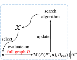
(a) Conventional methods

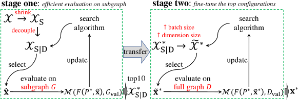
(b) KGTuner

Figure 1: The framework of conventional HP search algorithm and the proposed KGTuner.

Knowledge graph (KG) is a special kind of graph structured data to represent knowledge through entities and relations between the entities (Wang et al., 2017; Ji et al., 2021). Learning from KG aims to discover the latent properties from KGs to infer the existence of interactions among entities or the types of entities Wang et al. (2017); Zhang and Yao (2022). KG embedding, which encodes entities and relations as low dimensional vectors, is an important technique to learn from KGs (Wang et al., 2017; Ji et al., 2021). The existing models range from translational distance models (Bordes et al., 2013), tensor factorization models (Nickel et al., 2011; Trouillon et al., 2017; Balažević et al., 2019), neural network models (Dettmers et al., 2017; Guo et al., 2019), to graph neural networks (Schlichtkrull et al., 2018; Vashishth et al., 2020).

Hyper-parameter (HP) search (Claesen and De Moor, 2015) is very essential for KG learning. In this work, we take KG embedding methods Wang et al. (2017), as a good example to study the impact of HPs to KG learning. As studied, the HP configurations greatly influence the model performance (Ruffinelli et al., 2019; Ali et al., 2020). An improper HP configuration will impede the model from stable convergence, while an appropriate one can make considerable promotion to the model performance. Indeed, studying the HP configurations can help us make a more scientific understanding of the contributions made by existing works (Rossi et al., 2021; Sun et al., 2020). In addition, it is also important to search for an optimal HP configuration when adopting KG embedding methods to the real-world applications (Bordes et al., 2014; Zhang et al., 2016; Saxena et al., 2020).

Algorithms for HP search on general machine learning problems have been well-developed (Claesen and De Moor, 2015). As shown in Figure 1(a), the search algorithm selects a HP configuration from the search space in each iteration, then the evaluation feedback obtained by full model training is used to update the search algorithm. The optimal HP is the one achieving the best performance on validation data in the search process. Representative HP search algorithms are within sample-based methods like grid search, random search (Bergstra and Bengio, 2012), and sequential model-based Bayesian optimization (SMBO) methods like Hyperopt (Bergstra et al., 2013), SMAC (Hutter et al., 2011), Spearmint (Snoek et al., 2012) as well as BORE (Tiao et al., 2021), etc. Recently, some subgraph-based methods (Tu et al., 2019; Wang et al., 2021) are proposed to learn a predictor with configurations efficiently evaluated on small subgraphs The predictor is then transferred to guide HP search on the full graph. However, these methods fail to efficiently search a good configuration of HPs for KG embedding models since the training cost of individual model is high and the correlation of HPs in the huge search space is very complex.

To address the limitations of existing HP search algorithms, we carry a comprehensive understanding study on the influence and correlation of HPs as well as their transfer ability from small subgraph to full graph in KG learning. From the aspect of performance, we classify the HPs into four different groups including reduced options, shrunken range, monotonously related and no obvious patterns based on their influence on the performance. By analyzing the validation curvature of these HPs, we find that the space is rather complex such that only tree-based models can approximate it well. In addition, we observe that the consistency between evaluation on small subgraph and that on the full graph is high, while the evaluation cost is significantly smaller on the small subgraph.

Above understanding motivates us to reduce the size of search space and design a two-stage search algorithm named as KGTuner. As shown in Figure 1(b), KGTuner explores HP configurations in the shrunken and decoupled space with the search algorithm RF+BORE (Tiao et al., 2021) on a subgraph in the first stage, where the evaluation cost of HPs are small. Then in the second stage, the configurations achieving the top10 performance at the first stage are equipped with large batch size and dimension size for fine-tuning on the full graph.

Within the same time budget, KGTuner can consistently search better configurations than the baseline search algorithms for seven KG embedding models on WN18RR (Dettmers et al., 2017) and FB15k-237 (Toutanova and Chen, 2015). By applying KGTuner to the large-scale benchmarks ogbl-biokg and ogbl-wikikg2 (Hu et al., 2020), the performances of embedding models are improved compared with the reported results on OGB link prediction leaderboard. Besides, we justify the improvement of efficiency via analyzing the design components in KGTuner.

2 Background: HPs in KG embedding

We firstly revisit the important and common HPs in KG embedding. Following the general framework (Ruffinelli et al., 2019; Ali et al., 2020), the learning problem can be written as

$$\vspace{-2px}\!\!\!\!\bm{P}^{*}\!=\!\arg\min\nolimits_{\bm{P}}L(F(\cdot,\bm{P}),D^{+},D^{-})\!+\!r(\bm{P}),\vspace{-2px}$$ (1)

where $F$ is the form of an embedding model with learnable parameters $\bm{P}$, $D^{+}$ is the set of positive samples from the training data, $D^{-}$ represents negative samples, and $r(\cdot)$ is a regularization function. There are four groups of hyper-parameters (Table 1), i.e., the size of negative sampling for $D^{-}$, the choice of loss function $L$, the form of regularization $r(\cdot)$, and the optimization $\arg\min_{\bm{P}}$.

Table 1: The HP space. Conditioned HPs are in parenthesize. “adv.” and “reg.” are short for “adversarial” and “regularization”, respectively. Please refer to the Appendix A for more details.

component	name	type	range
negative sampling	# negative samples	cat	{32, 128, 512, 2048, 1VsAll, kVsAll}
loss function	loss function	cat	{MR, BCE_(mean, sum, adv), CE}
	gamma (MR)	float	[1, 24]
	adv. weight (BCE_adv)	float	[0.5, 2.0]
regularization	regularizer	cat	{FRO, NUC, DURA, None}
	reg. weight (not None)	float	[$10^{-12}$, $10^{2}$]
	dropout rate	float	$[0,0.5]$
optimization	optimizer	cat	{Adam, Adagrad, SGD}
	learning rate	float	[$10^{-5}$, $10^{0}$]
	initializer	cat	{uniform, normal, xavier_uniform, xavier_norm}
	batch size	int	{128, 256, 512, 1024}
	dimension size	int	{100, 200, 500, 1000, 2000}
	inverse relation	bool	{True, False}

Embedding model. While there are many existing embedding models, we follow (Ruffinelli et al., 2019) to focus on some representative models. They are translational distance models TransE (Bordes et al., 2013) and RotatE (Sun et al., 2019), tensor factorization models RESCAL (Nickel et al., 2011), DistMult (Yang et al., 2015), ComplEx (Trouillon et al., 2017) and TuckER (Balažević et al., 2019), and neural network models ConvE (Dettmers et al., 2017). Graph neural networks for KG embedding (Schlichtkrull et al., 2018; Vashishth et al., 2020; Zhang and Yao, 2022) are not studied here for their scalability issues on large-scale KGs (Ji et al., 2021).

Negative sampling. Sampling negative triplets is important as only positive triplets are contained in the KGs (Wang et al., 2017). We can pick up $m$ triplets by replacing the head or tail entity with uniform sampling (Bordes et al., 2013) or use a full set of negative triplets. Using the full set can be defined as the 1VsAll (Lacroix et al., 2018) or kVsAll (Dettmers et al., 2017) according to the positive triplets used. The methods Cai and Wang (2018); Zhang et al. (2021) requiring additional models for negative sampling are not considered here.

Loss function. There are three types of loss functions. One can use margin ranking (MR) loss (Bordes et al., 2013) to rank the positive triplets higher over the negative ones, or use binary cross entropy (BCE) loss, with variants BCE_mean, BCE_adv (Sun et al., 2019) and BCE_sum (Trouillon et al., 2017), to classify the positive and negative triplets as binary classes, or use cross entropy (CE) loss (Lacroix et al., 2018) to classify the positive triplet as the true label over the negative triplets.

Regularization. To balance the expressiveness and complexity, and to avoid unbounded embeddings, the regularization techniques can be considered, such as regularizers like Frobenius norm (FRO) (Yang et al., 2015; Trouillon et al., 2017), Nuclear norm (NUC) (Lacroix et al., 2018) as well as DURA (Zhang et al., 2020b), and dropout on the embeddings (Dettmers et al., 2017).

Optimization. To optimize the embeddings, important optimization choices include the optimizer, such as SGD, Adam (Kingma and Ba, 2014) and Adagrad (Duchi et al., 2011), learning rate, initializers, batch size, embedding dimension size, and add inverse relation (Lacroix et al., 2018) or not.

3 Defining the search problem

Denote an instance $\mathbf{x}=(x_{1},x_{2}\dots,x_{n})$, which is called an HP configuration, in the search space $\mathcal{X}$. Let $F(\bm{P},\mathbf{x})$ be an embedding model with model parameters $\bm{P}$ and HPs $\mathbf{x}$, we define $\mathcal{M}(F(\bm{P},\mathbf{x}),D_{\text{val}})$ as the performance measurement (the larger the better) on validation data $D_{\text{val}}$ and $\mathcal{L}(F(\bm{P},\mathbf{x}),D_{\text{tra}})$ as the loss function (the smaller the better) on training data $D_{\text{tra}}$. We define the problem of HP search for KG embedding models in Definition 1. The objective is to search an optimal configuration $\mathbf{x}^{*}\in\mathcal{X}$ such that the embedding model $F$ can achieve the best performance on the validation data $D_{\text{val}}$.

Definition 1 (Hyper-parameter search for KG embedding).

The problem of HP search for KG embedding model is formulated as

$$\vspace{-2px}\mathbf{x}^{*} =\arg\max\nolimits_{\mathbf{x}\in\mathcal{X}}\mathcal{M}\big{(}F(\bm{P}^{*},\mathbf{x}),D_{\text{val}}\big{)},$$ (2)

$$\bm{P}^{*} =\arg\min\nolimits_{\bm{P}}\mathcal{L}\big{(}F(\bm{P},\mathbf{x}),D_{\text{tra}}\big{)}.\vspace{-2px}$$ (3)

Definition 1 is a bilevel optimization problem (Colson et al., 2007), which can be solved by many conventional HP search algorithms. The most common and widely used approaches are sample-based methods like grid search and random search (Bergstra and Bengio, 2012), where the HP configurations are independently sampled. To guide the sampling of HP configurations by historical experience, SMBO-based methods (Bergstra et al., 2011; Hutter et al., 2011) learn a surrogate model to select configurations based on the results that have been evaluated. Then, the model parameters $\bm{P}$ are optimized by minimizing the loss function $\mathcal{L}$ on $D_{\text{tra}}$ in Eq. (3). The evaluation feedback $\mathcal{M}$ of $\mathbf{x}$ on the validation data $D_{\text{val}}$ is used to update the surrogate.

Figure 2: Ranking distribution of selected HPs. A value with larger area in the bottom indicates the higher ranking of this value. The four figures correspond to the four groups: reduced options, shrunken range, monotonously related, no obvious patterns. Full results are in the Appendix B.2.

There are three major aspects determining the efficiency of Definition 1: (i) the size of search space $\mathcal{X}$, (ii) the validation curvature of $\mathcal{M}(\cdot,\cdot)$ in Eq. (2), and (iii) the evaluation cost in solving $\arg\min_{\bm{P}}\mathcal{L}$ in Eq. (3). However, the existing methods Ruffinelli et al. (2019); Ali et al. (2020) directly search on a huge space with commonly used surrogate models and slow evaluation feedback from the full KG due to the lack of understanding on the search problem, leading to low efficiency.

4 Understanding the search problem

To address the mentioned limitations, we measure the significance and correlation of each HP to determine the feasibility of the search space $\mathcal{X}$ in Section 4.1. In Section 4.2, we visualize the HPs that determine the curvature of Eq. (2). To reduce the evaluation cost in Eq.  (3), we analyze the approximation methods in Section 4.3. Following (Ruffinelli et al., 2019), the experiments run on the seven embedding models in Section 2 and two widely used datasets WN18RR (Dettmers et al., 2017) and FB15k-237 (Toutanova and Chen, 2015). The experiments are implemented with PyTorch framework (Paszke et al., 2017), on a machine with two Intel Xeon 6230R CPUs and eight RTX 3090 GPUs with 24 GB memories each. We provide the implementation details in the Appendix D.1.

4.1 Search space: $\mathbf{x}\in\mathcal{X}$

Considering such large amount of HP configurations in $\mathcal{X}$, we take the simple and efficient approach where HPs are evaluated under control variate (Hutter et al., 2014; You et al., 2020), which varies the $i$-th HP while fixing the other HPs. First, we discretize the continuous HPs according to their ranges. Then the feasibility of the search space $\mathcal{X}$ is analyzed by checking the ranking distribution and consistency of individual HPs. These can help us shrink and decouple the search space. The detailed setting for this part is in the Appendix B.1.

Ranking distribution. To shrink the search space, we use the ranking distribution to indicate what HP values perform consistently. Given an anchor configuration $\mathbf{x}$, we obtain the ranking of different values $\theta\in X_{i}$ by fixing the other HPs, where $X_{i}$ is the range of the $i$-th HP. The ranking distribution is then collected over the different anchor configurations in $\mathcal{X}_{i}$, different models and datasets. According to the violin plots of ranking distribution shown in Figure 2, the HPs can be classified into four groups:

• reduced options, e.g., Adam is the best optimizer and inverse relation should not be introduced;

• shrunken range, e.g., learning rate, reg. weight and dropout rate are better in certain ranges;

• monotonously related: e.g., larger batch size and dimension size tend to be better;

• no obvious patterns: e.g., the remaining HPs.

Consistency. To decouple the search space, we measure the consistency of configurations’ rankings when only a specific HP changes. For the $i$-th HP, if the ranking of configurations’ performance is consistent with different values of $\theta\in X_{i}$, we can decouple the search procedure of the $i$-th HP with the others. We measure such consistency with the spearman’s ranking correlation coefficient (SRCC) (Schober et al., 2018).

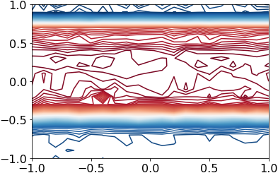
(a) Ground truth

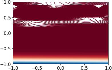
(b) GP prediction

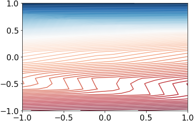
(c) MLP prediction

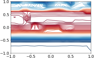
(d) RF prediction

Figure 3: Curvature of the search space and three surrogate models. The search space curvature is quite complex with many local maximum areas. The curvature of RF approximate the ground truth best.

Given a value $\theta\in X_{i}$, we obtain the ranking $r(\mathbf{x},\theta)$ of the anchor configurations $\mathbf{x}\in\mathcal{X}_{i}$ by fixing the $i$-th HP as $\theta$. Then, the SRCC between the two HP values $\theta_{1},\theta_{2}\in X_{i}$ is computed as

$$1-\frac{\sum_{\mathbf{x}\in\mathcal{X}_{i}}\!|r(\mathbf{x},\theta_{1})\!-\!r(\mathbf{x},\theta_{2})|^{2}}{|\mathcal{X}_{i}|\cdot(|\mathcal{X}_{i}|^{2}-1)},\vspace{-1px}$$ (4)

where $|\mathcal{X}_{i}|$ means the number of anchor configurations in $\mathcal{X}_{i}$. SRCC indicates the matching rate of rankings for the anchor configurations in $\mathcal{X}_{i}$ with respect to $x_{i}=\theta_{1}$ and $x_{i}=\theta_{2}$. Then the consistency of the $i$-th HP is evaluated by averaging the SRCC over the different pairs of $(\theta_{1},\theta_{2})$ for $X_{i}$, the different models and different datasets. The larger consistency (in the range $[-1,1]$) indicates that changing the value of the $i$-th HP does not influence much on the other configurations’ ranking.

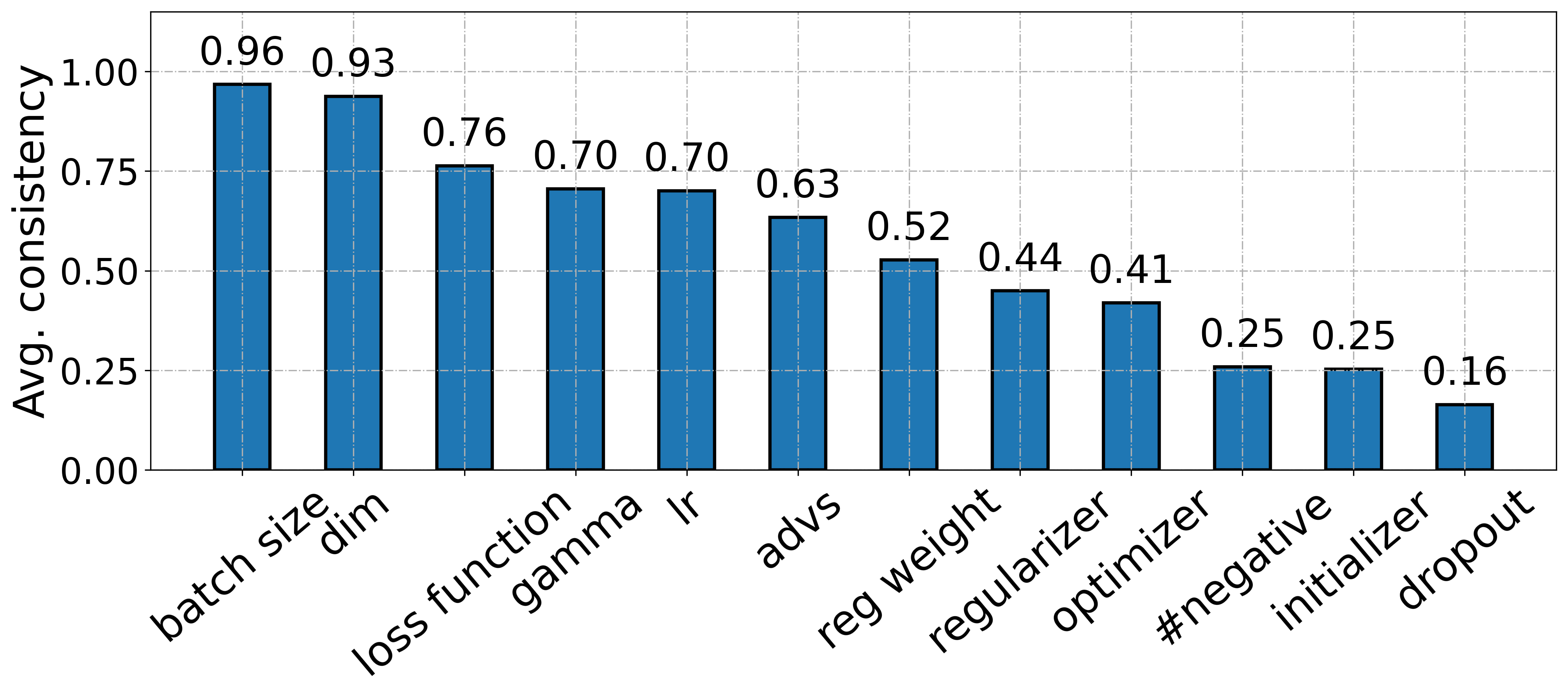
Figure 4: Consistency of each HP.

As in Figure 4, the batch size and dimension size show higher consistency than the other HPs. Hence, the evaluation of the configurations can be consistent with different choices of the two HPs. This indicates that we can decouple the search of batch size and dimension size with the other HPs.

4.2 Validation curvature: $\mathcal{M}(\cdot,\cdot)$

We analyze the curvature of the validation performance $\mathcal{M}(\cdot,\cdot)$ w.r.t $\mathbf{x}\in\mathcal{X}$. Specifically, we follow (Li et al., 2017) to visualize the validation loss’ landscape by uniformly varying the numerical HPs in two directions (20 configurations in each direction) on the model ComplEx and dataset WN18RR. From Figure 3(a), we observe that the curvature is quite complex with many local maximum areas.

To gain insights from evaluating these configurations and guide the next configuration sampling, we learn a surrogate model as the predictor to approximate the validation curvature. The curvatures of three common surrogates, i.e., Gaussian process (GP) (Williams and Rasmussen, 1995), multi-layer perceptron (MLP) (Gardner and Dorling, 1998) and random forest (RF) (Breiman, 2001), are in Figures 3(b)-3(d). The surrogate models are trained with the evaluations of $100$ random configurations in the search space. As shown, both GP and MLP fail to capture the complex local surface in Figure 3(a) as they tend to learn a flat and smooth distribution in the search space. In comparison, RF is better in capturing the local distributions. Hence, we regard RF as a better choice in the search space. A more detailed comparison on the approximation ability of different surrogates is in the Appendix B.3.

4.3 Evaluation cost: $\arg\min_{\bm{P}}\mathcal{L}$

The evaluation cost of the HP configuration on an embedding model is the majority computation cost in HP search. Thus, we firstly evaluate the HPs that have influence on the evaluation cost, including batch size, dimension size, number of negative samples loss function and regularizer. Then, we analyze the evaluation transfer ability from small subgraph to the full graph.

Cost of different HPs. The cost of each HP value $\theta\in X_{i}$ is averaged over the different anchor configurations in $\mathcal{X}_{i}$, different models and datasets. For fair comparsion, the time cost is counted per thousand iterations. We find that the evaluation cost increases significantly with larger batch size and dimension size, while the number of negative samples and the choice of loss function or regularizer do not have much influence on the cost. We provide two exemplar curves in Figure 5 and put the remaining results in the Appendix B.4.

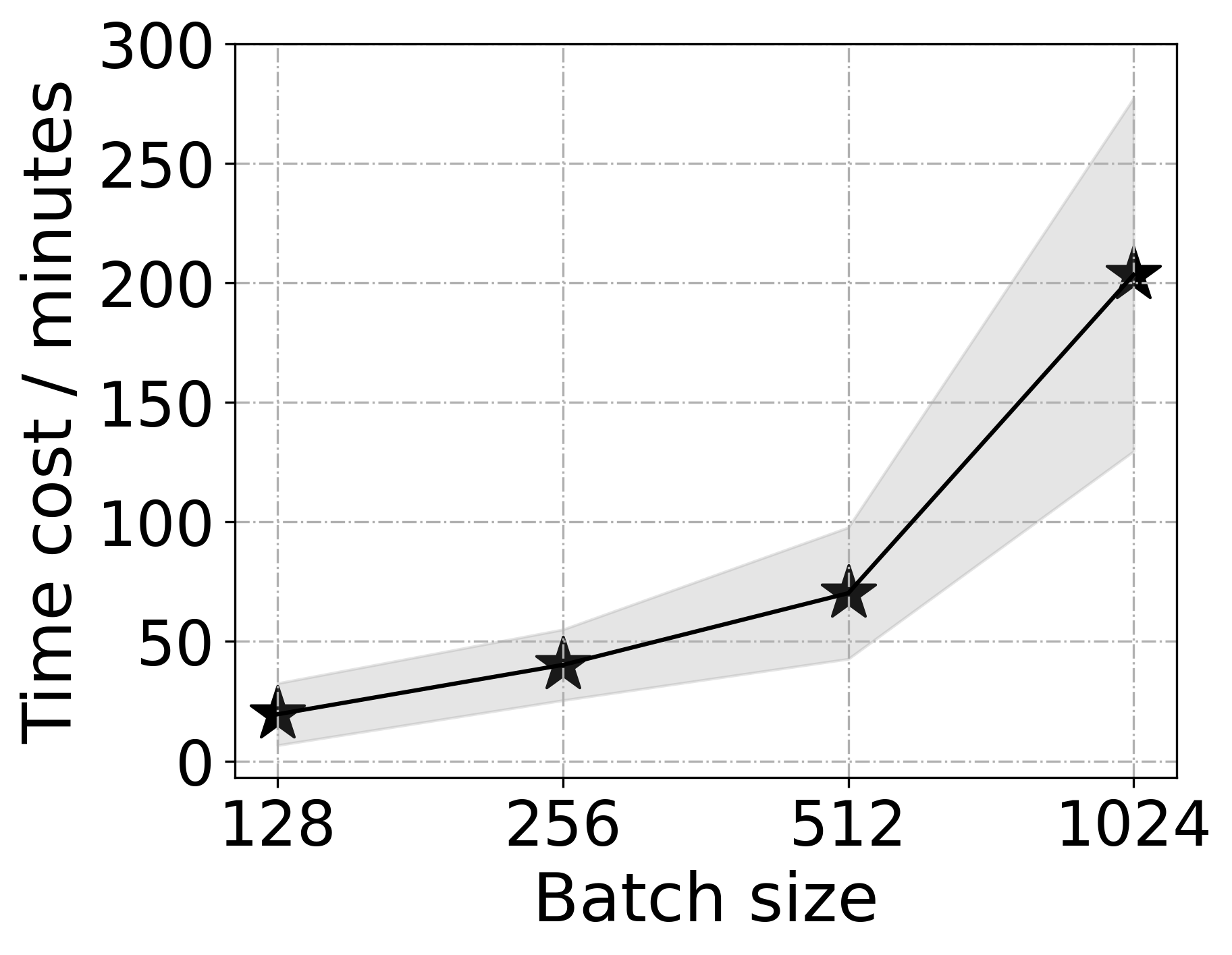
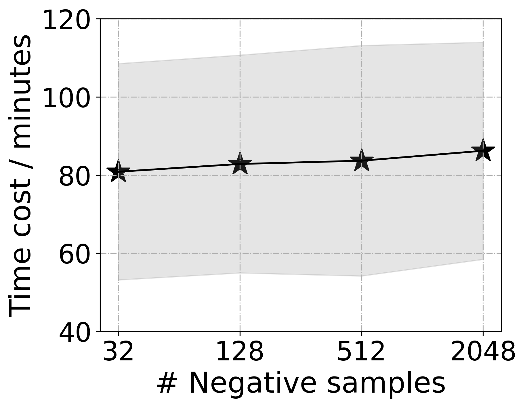
Figure 5: Computing time cost. The dots are the average and the shades are the standard deviation.

Transfer ability of subgraphs. Subgraphs can efficiently approximate the properties of the full graph (Hamilton et al., 2017; Teru et al., 2020). We evaluate the impact of subgraph sampling on HP search by checking the consistency between evaluations results on small subgraph and those on the full graph.

First, we study how to sample subgraphs. There are several approaches to sample small subgraphs from a large graph Leskovec and Faloutsos (2006). We compare four representative approaches in Figure 6, i.e., Pagerank node sampling (Pagerank), random edge sampling (Random Edge), single-start random walk (Single-RW) and multi-start random walk (Multi-RW). For a fair comparison, we constrain the subgraphs with about $20\%$ of the full graph. The consistency between the sampled subgraph with the full graph is evaluated by the SRCC in (4). We observe that multi-start random walk is the best among the different sampling methods.

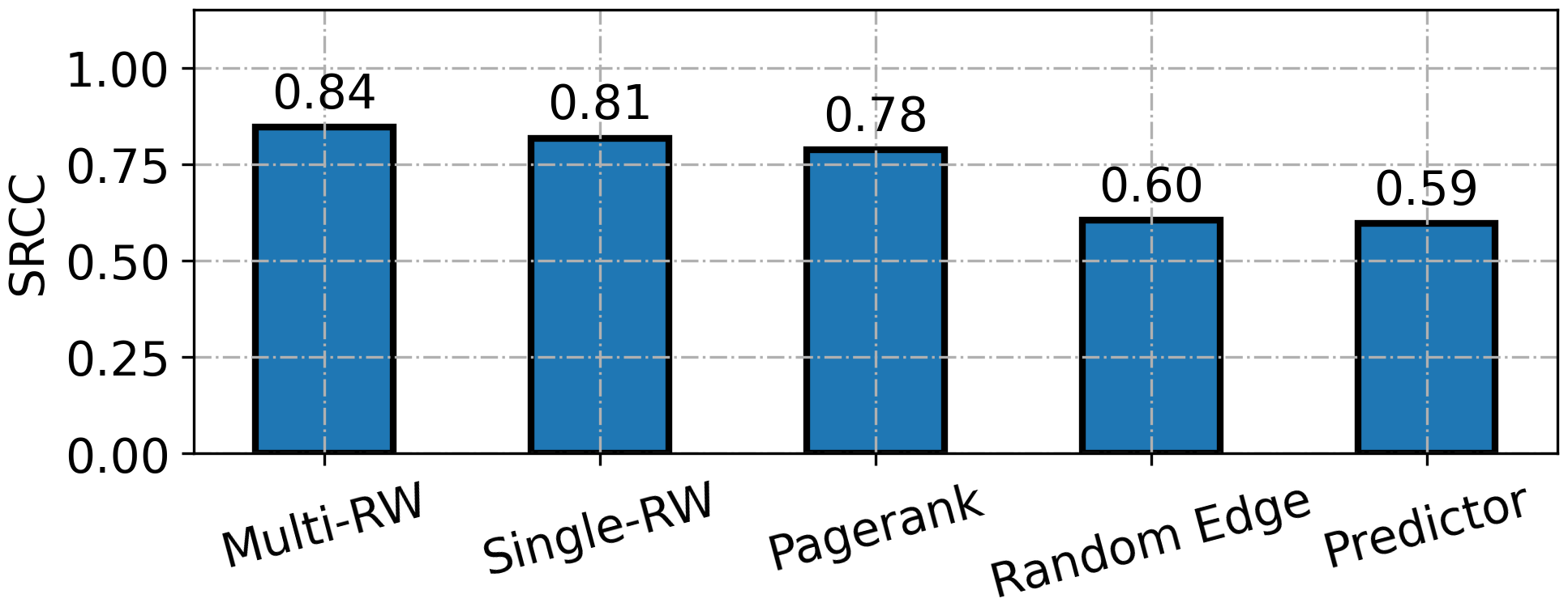
Figure 6: Comparison of the sampling methods.

Apart from directly transferring the evaluation from subgraph to full graph, we can alternatively train a predictor with observations on subgraphs and then transfers the model to predict the configuration performance on the full graph. From Figure 6, we find that directly transferring evaluations from subgraphs to the full graph is much better than transferring the predictor model.

In addition, we show the consistency and cost in terms of different subgraph sizes (percentage of entities compared to the full graph) in Figure 7. As shown, evaluation on subgraphs can significantly improve the efficiency. When the scale increases, the consistency increases but the cost also increases. To balance the consistency and cost, the subgraphs with $20\%$ entities are the better choices.

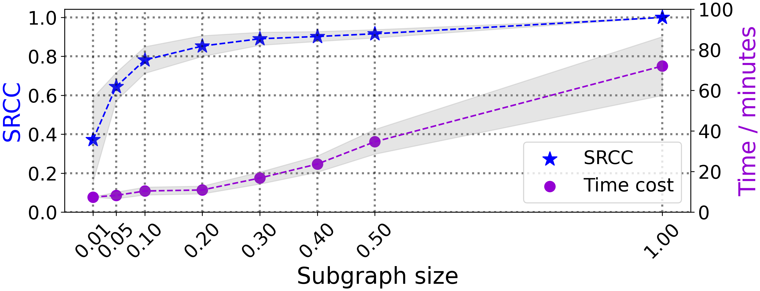
Figure 7: Consistency and cost of different subgraph sizes, where the shades are the standard deviation.

5 Efficient search algorithm

By analyzing the ranking distribution and consistency of HPs in Section 4.1, we observe that not all the HP values are equivalently good, and some HPs can be decoupled. These observations motivate us to revise the search space in Section 5.1. Based on the analysis in Section 4.2 and 4.3, we then propose an efficient two-stage search algorithm in Section 5.2.

5.1 Shrink and decouple the search space

To shrink the search space, we mainly consider groups (a) and (b) of HPs in Section 4.1. From the full results in the Appendix B.2, we observe that Adam can consistently perform better than the other two optimizers, the learning rate is better in the range of $[10^{-4},10^{-1}]$, the regularization weight is better in $[10^{-8},10^{-2}]$, dropout rate is better in $[0,0.3]$, and add inverse relation is not a good choice.

To decouple the search space, we consider batch size and dimension size that have larger consistency values than the other HPs, and are monotonously related to the performance as in group (c). However, the computation costs of batch size and dimension size increase prominently as shown in Figure 5. Hence, we can set batch size as 128 and dimension size as 100 to search the other HPs with low evaluation cost and increase their values in a fine-tuning stage.

Given the full search space $\mathcal{X}$, we denote the shrunken space as ${\mathcal{X}}_{\text{S}}$ and the further decoupled space as ${\mathcal{X}}_{\text{S|D}}$. We achieve hundreds of times size reduction from ${\mathcal{X}}_{\text{S}}$ to ${\mathcal{X}}_{\text{S|D}}$ and we show the details of changes in the Appendix C.

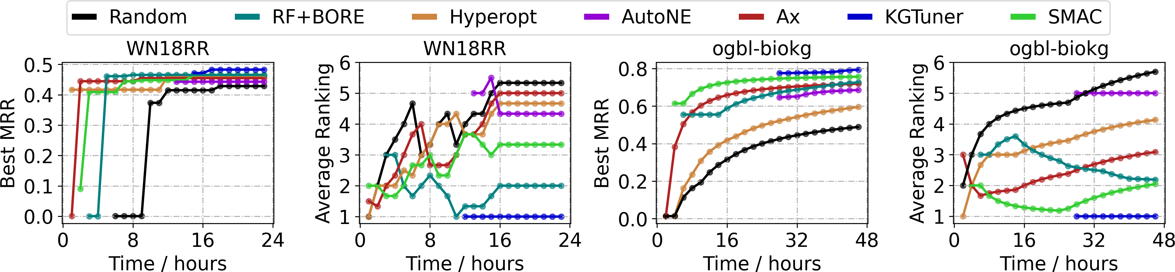
Figure 8: Search algorithm comparison (viewed in color). The dots are the results collected per hour.

5.2 Two-stage search algorithm (KGTuner)

As discussed in Section 4.3, the evaluation cost can be significantly reduced with small batch size, dimension size and subgraph. This motivates us to design a two-stage search algorithm, named KGTuner, as in Figure 1(b) and Algorithm 1.

Algorithm 1 KGTuner: two-stage search algorithm

0:  KG embedding model $F$, dataset $D$, and budget $B$;

1:  shrink the search space $\mathcal{X}$ to ${\mathcal{X}}_{\text{S}}$ and decouple ${\mathcal{X}}_{\text{S}}$ to ${\mathcal{X}}_{\text{S|D}}$; # state one: efficient evaluation on subgraph

2:  sample a subgraph (with $20\%$ entities) $G$ from $D_{\text{tra}}$ by multi-start random walk;

3:  repeat

4:     sample a configuration $\hat{\mathbf{x}}$ from ${\mathcal{X}}_{S|D}$ by RF+BORE;

5:     evaluate $\hat{\mathbf{x}}$ on the subgraph $G$ to get the performance;

6:     update the RF with record $\big{(}\hat{\mathbf{x}},\mathcal{M}(F(P^{*},\hat{\mathbf{x}}),G_{\text{val}})\big{)}$;

7:  until $\nicefrac{{B}}{{2}}$ budget exhausted;

8:  save the top10 configurations in ${\mathcal{X}}_{\text{S|D}}^{*}$; # state two: fine-tune the top configurations

9:  increase the batch/dimension size in ${\mathcal{X}}_{\text{S|D}}^{*}$ to get $\tilde{\mathcal{X}}^{*}$;

10:  set $y^{*}=0$ and re-initialize the RF surrogate;

11:  repeat

12:     select a configuration $\tilde{\mathbf{x}}^{*}$ from $\tilde{\mathcal{X}}^{*}$ by RF+BORE;

13:     evaluate on full graph $G$ to get the performance;

14:     update the RF with record $\big{(}\tilde{\mathbf{x}}^{*}\!\!,\mathcal{M}(F(P^{*}\!,\tilde{\mathbf{x}}^{*}),\!D_{\text{val}})\!\big{)}$;

15:     if $\mathcal{M}(F(P^{*},\tilde{\mathbf{x}}^{*}),D_{\text{val}})>y^{*}$ then $y^{*}\!\leftarrow\mathcal{M}(F(P^{*},\tilde{\mathbf{x}}^{*}),D_{\text{val}})$ and $\mathbf{x}^{*}\leftarrow\tilde{\mathbf{x}}^{*}$; end if

16:  until the remaining $\nicefrac{{B}}{{2}}$ budget exhausted;

17:  return  $\mathbf{x}^{*}$.

• In the first stage, we sample a subgraph $G$ with $20\%$ entities from the full graph $D_{\text{tra}}$ by multi-start random walk. Based on the understanding of curvature in Section 4.2, we use the surrogate model random forest (RF) under the state-of-the art framework BORE Tiao et al. (2021), denoted as RF+BORE, to explore HPs in ${\mathcal{X}}_{\text{S|D}}$ on the subgraph $G$ in steps 3-7. The top10 configurations evaluated in this stage are saved in a set ${\mathcal{X}}^{*}_{\text{S|D}}$.

• In the second stage, we increase batch size and dimension size for configurations in ${\mathcal{X}}^{*}_{\text{S|D}}$ to generate a new set $\tilde{\mathcal{X}}^{*}$. Then, the configurations in $\tilde{\mathcal{X}}^{*}$ are searched by the RF+BORE again in steps 11-16 until the remaining $\nicefrac{{B}}{{2}}$ budget is exhausted.

• Finally, the configuration $\mathbf{x}^{*}$ achieving the best performance on the full validation data $D_{\text{val}}$ is returned for testing.

5.3 Discussion

e now summarize the main differences of KGTuner with the existing HP search algorithms, i.e. Random (random search) (Bergstra and Bengio, 2012), Hyperopt Bergstra et al. (2013), SMAC (Hutter et al., 2011), RF+BORE (Tiao et al., 2021), and AutoNE (Tu et al., 2019).

Table 2: Comparison of HP search algorithms.

	search space		surrogate	fast
	shrink	decouple	model	evaluation
Random	$\times$	$\times$	$\times$	$\times$
Hyperopt	$\times$	$\times$	TPE	$\times$
Ax	$\times$	$\times$	GP	$\times$
SMAC	$\times$	$\times$	RF	$\times$
RF+BORE	$\times$	$\times$	RF	$\times$
AutoNE	$\times$	$\times$	GP	$\surd$
KGTuner	$\surd$	$\surd$	RF	$\surd$

The comparison is based on three aspects, i.e., search space, surrogate model and fast evaluation, in Table 2. KGTuner shrinks and decouples the search space based on the understanding of HPs’ properties, and uses the surrogate RF based on the understanding on validation curvature. The fast evaluation on subgraph in KGTuner selects the top10 configurations to directly transfer for fine-tuning, while AutoNE (Tu et al., 2019) just uses fast evaluation on subgraphs to train the surrogate model, and transfers the surrogate model for HP search on the full graph. In Figure 6, the transfer ability of the surrogate model is shown to be much worse than direct transferring.

6 Empirical evaluation

6.1 Overall performance

In this part, we compare the proposed algorithm KGTuner with six HP search algorithms in Table 2. For AutoNE, we allocate half budget for it to search on the subgraph and another half budget on the full graph with the transferred surrogate model. The baselines search in the full search space (in Table 1) with the same amount of budget as KGTuner. We use the mean reciprocal ranking (MRR, the larger the better) (Bordes et al., 2013) to indicate the performance.

Efficiency. We compare the different search algorithms in Figure 8 on an in-sample dataset WN18RR and an out-of-sample dataset ogbl-biokg. The time budget we set for WN18RR is one day’s clock time, while that for ogbl-biokg is two days’ clock time. For each dataset we show two kinds of figures. First, the best performance achieved along the clock time in one experiment on a specific model ComplEx. Second, we plot the the ranking of each algorithm averaged over all the models and datasets. Since AutoNE and KGTuner run on the subgraphs in the first stage, the starting points of them locate after 12 hours. The starting point of KGTuner is a bit later than AutoNE since it constrains to use large batch size and dimension size in the second stage, which is more expensive. As shown, random search is the worst. SMAC and RF+BORE achieve better performance than Hyperopt and Ax since RF can fit the space better than TPE and GP as in Section 4.2. Due to the weak transfer ability of the predictor (see Figure 6) and the weak approximation ability of GP (see Figure 3), AutoNE also performs bad. KGTuner is much better than all the baselines. We show the full search process of the two-stage algorithms AutoNE and KGTuner on WN18RR in Figure 9(a). By exploring sufficient number of configurations in the first stage, the configurations fine-tuned in the second stage can consistently achieve the best performance.

Effectiveness. For WN18RR and FB15k-237, we provide the reproduced results on TransE, ComplEx and ConvE with the original HPs, HPs searched by LibKGE and HPs searched by KGTuner in Table 3. The full results on the remaining four embedding models RotatE, RESCAL, DistMult and TuckER are in the Appendix D.2. Overall, KGTuner achieves better performance compared with both the original reported results and the reproduced results in (Ruffinelli et al., 2019). We observe that the tensor factorization models such as RESCAL, ComplEx and TuckER have better performance than the translational distance models TransE, RotatE and neural network model ConvE. This conforms with the theoretical analysis that tensor factorization models are more expressive (Wang et al., 2018).

Table 3: MRR of models with HPs tuned in different methods. The bold numbers mean the best performance of the same model.

source	models	WN18RR	FB15k-237
original	TransE	0.226	0.296
	ComplEx	0.440	0.247
	ConvE	0.430	0.325
LibKGE	TransE	0.228	0.313
	ComplEx	0.475	0.348
	ConvE	0.442	0.339
KGTuner	TransE	0.233	0.327
	ComplEx	0.484	0.352
	ConvE	0.437	0.335

(a) Full search processes

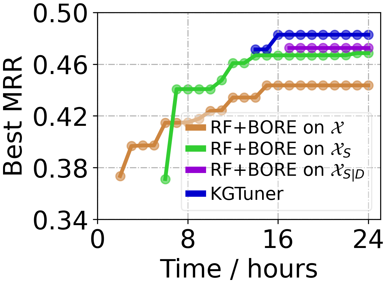
(b) Search space

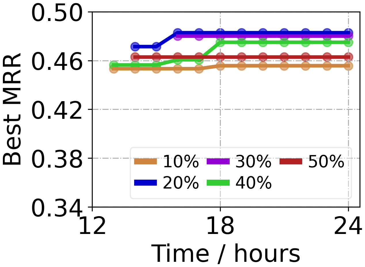
(c) Subgraph size

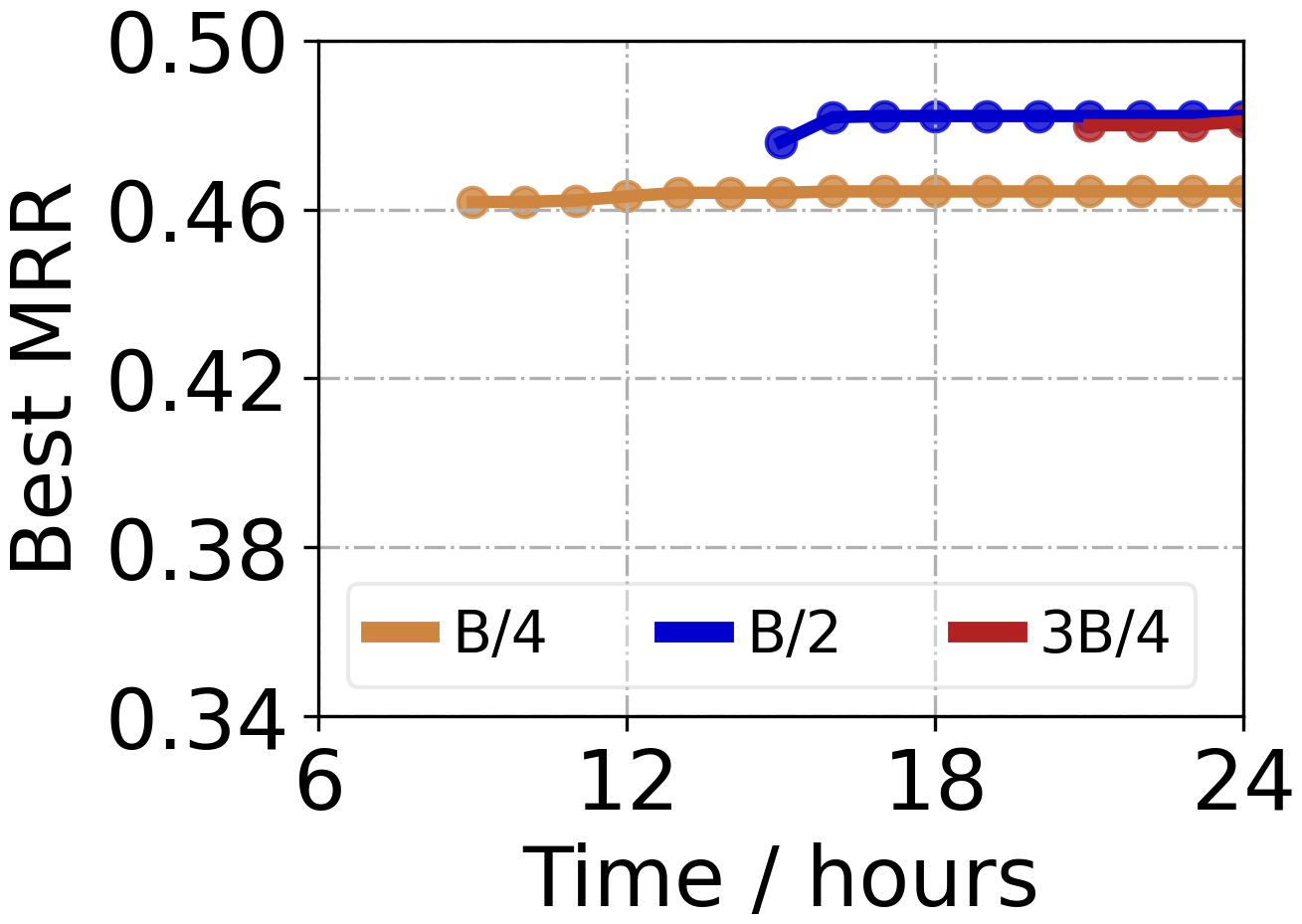
(d) First-stage budget

Figure 9: (a): full search processes of the two-stage algorithms. (b-d): ablation studies on KGTuner. Model ComplEx and dataset WN18RR are used in these experiments.

To further demonstrate the advantage of KGTuner, we apply it to the Open Graph Benchmark (OGB) (Hu et al., 2020), which is a collection of realistic and large-scale benchmark datasets for machine learning on graphs. Many embedding models have been tested there by two large-scale KGs for link prediction, i.e., ogbl-biokg and ogbl-wikikg2. Due to their scale, the evaluation cost of a HP configuration is very expensive. We use KGTuner to search HPs for embedding models, i.e., TransE, RotatE, DistMult, ComplEx and AutoSF Zhang et al. (2020a), on OGB. Since the computation costs of the two datasets are much higher, we set the time budget as 2 days for ogbl-biokg and 5 days for ogbl-wikikg2. All the embedding models evaluated here are constrained to have the same (or lower) number of model parameters. More details on model parameters, standard derivation, and validation performance are in the Appendix D.3. As shown in Table 4, KGTuner consistently improves the performance of the four embedding models with the same or fewer parameters compared with the results on the OGB board.

Table 4: Performance in MRR in OGB link prediction board https://ogb.stanford.edu/docs/leader_linkprop/ and those reproduced by KGTuner on ogbl-biokg and ogbl-wikikg2. Relative improvements are in parenthesize.

models		ogbl-biokg	ogbl-wikikg2
	TransE	0.7452	0.4256
	RotatE	0.7989	0.2530
original	DistMult	0.8043	0.3729
	ComplEx	0.8095	0.4027
	AutoSF	0.8320	0.5186
	TransE	0.7781 (4.41%$\uparrow$)	0.4739 (11.34%$\uparrow$)
	RotatE	0.8013 (0.30%$\uparrow$)	0.2944 (16.36%$\uparrow$)
KGTuner	DistMult	0.8241 (2.46%$\uparrow$)	0.4837 (29.71%$\uparrow$)
	ComplEx	0.8385 (3.58%$\uparrow$)	0.4942 (22.72%$\uparrow$)
	AutoSF	0.8354 (0.41%$\uparrow$)	0.5222 (0.69%$\uparrow$)
average improvement		2.23%	16.16%

6.2 Ablation study

In this subsection, we probe into how important and sensitive the various components of KGTuner are.

Space comparison. To demonstrate the effectiveness gained by shrinking and decoupling the search space, we compare the following variants: (i) RF+BORE on the full space $\mathcal{X}$; (ii) RF+BORE on the shrunken space ${\mathcal{X}}_{\text{S}}$; (iii) RF+BORE on the decoupled space ${\mathcal{X}}_{\text{S|D}}$, which differs from KGTuner by searching on the full graph in the first stage; and (iv) KGTuner in Algorithm 1. All the variants, i.e., RF+BORE, have one day’s time budget. As in Figure 9(b), the size of search space matters for the search efficiency. The three components, i.e., space shrinkage, space decoupling, and fast evaluation on subgraph, are all important to the success of KGTuner.

Size of subgraphs. We show the influence of subgraph sizes with different ratios of entities (10%, 20%, 30%, 40%, 50%) from the full graph in Figure 9(c). Using subgraphs with too large or too small size is not guaranteed to find good configurations. Based on the understanding in Figure 7, the subgraph with small size have poor transfer ability and those with large size are expensive to evaluate. Hence, we should balance the transfer ability and evaluation cost by sampling subgraphs with $20\%\sim 30\%$ entities.

Budget allocation. In Algorithm 1, we allocate $\nicefrac{{B}}{{2}}$ budget for both the first and second stage. Here, we show the performance of different allocation ratios, i.e., $\nicefrac{{B}}{{4}}$, $\nicefrac{{B}}{{2}}$, and $\nicefrac{{3B}}{{4}}$ in the first stage and the remaining budget in the second stage. As in Figure 9(d), allocating too many or too few budgets to the first stage is not good. It either fails to explore sufficient configurations in the first stage or only fine-tunes a few configurations in the second stage. Allocating the same budget to the two stages is in a better trade-off.

7 Related works

In analyzing the performance of KG embedding models, Ruffinelli et al. (2019) pointed out that the earlier works in KG embedding only search HPs in small grids. By searching hundreds of HPs in a unified framework, the reproduced performance can be significantly improved. Similarly, Ali et al. (2020) proposed another unified framework to evaluate different models. Rossi et al. (2021) evaluated 16 different models and analyzed their properties on different datasets. All of these works emphasize the importance of HP search, but none of them provide efficient algorithms to search HPs for KG learning. AutoSF (Zhang et al., 2020a) evaluates the bilinear scoring functions and set up a search problem to design bilinear scoring functions, which can be complementary to KGTuner.

Understanding the HPs in a large search space is non-trivial since many HPs only have moderate impact on the model performance Ruffinelli et al. (2019) and jointly evaluating them requires a large number of experiments (Fawcett and Hoos, 2016; Probst et al., 2019). Considering the huge amount of HP configurations (with $10^{5}$ categorical choices and $5$ continuous values), it is extremely expensive to exhaustively evaluate most of them. Hence, we adopt control variate experiments to efficiently evaluate HPs’ properties instead of the quasi-random search in (Ruffinelli et al., 2019; Ali et al., 2020).

Technically, we are similar to AutoNE (Tu et al., 2019) and e-AutoGR (Wang et al., 2021) by leveraging subgraphs to improve search efficiency on graph learning. Since they do not target at KG embedding methods, directly adopt them is not a good choice. Besides, based on the understanding in this paper, we demonstrate that transferring the surrogate model from subgraph evaluation to the full graph is inferior to directly transferring the top configurations for KG embedding models.

8 Conclusion

In this paper, we analyze the HPs’ properties in KG embedding models with search space size, validation curvature and evaluation cost. Based on the observations, we propose an efficient search algorithm KGTuner that efficiently explores configurations in a reduced space on small subgraph and then fine-tunes the top configurations with increased batch size and dimension size on the full graph. Empirical evaluations show that KGTuner is robuster and more efficient than the existing HP search algorithms and achieves competing performance on large-scale KGs in open graph benchmarks. In the future work, we will understand the HPs in graph neural network based models and apply KGTuner on them to solve the scaling limitations in HP search.

Appendix A Details of the search space

Denote a knowledge graph as $\mathcal{G}=\{E,R,D\}$, where $E$ is the set of entities, $R$ is the set of relations, and $D$ is the set of triplets with training/validation/test splits $D=D_{\text{tra}}\cup D_{\text{val}}\cup D_{\text{tst}}$.

Basically, the KG embedding models use a scoring function $f$ and the model parameters $\bm{P}$ to measure the plausibility of triplets. We learn the embeddings such that the positive and negative triplets can be separated by $f$ and $\bm{P}$. In Table 5, we provide the forms $f$ of the embedding model we used to evaluate the search space $\mathcal{X}$ in Section 3.

Table 5: Definitions of the embedding models. $\circ$ is a rotation operation in the complex value space; $\otimes$ is the Hermitian dot product in the complex value space; $\text{Re}(\cdot)$ returns the real part of a complex value; $\mathcal{W}_{i,j,k}$ is the $ijk$-th element in a core tensor $\mathcal{W}\in\mathbb{R}^{d\times d\times d}$; and conv is a convolution operator on the head and relation embeddings. For more details, please refer to the corresponding references.

model type	model	$f(h,r,t)$	embeddings
translational distance	TransE (Bordes et al., 2013)	$-\|\bm{h}+\bm{r}-\bm{t}\|_{1}$	$\bm{h},\bm{r},\bm{t}\in\mathbb{R}^{d}$
	RotatE (Sun et al., 2019)	$-\|\bm{h}\circ\bm{r}-\bm{t}\|_{c1}$	$\bm{h},\bm{r},\bm{t}\in\mathbb{C}^{d}$
tensor factorization	RESCAL (Nickel et al., 2011)	$\bm{h}^{\top}\cdot\bm{R}_{r}\cdot\bm{t}$	$\bm{h},\bm{t}\in\mathbb{R}^{d},\bm{R}_{r}\in\mathbb{R}^{d\times d}$
	DistMult (Yang et al., 2015)	$\bm{h}^{\top}\cdot\text{diag}(\bm{r})\cdot\bm{t}$	$\bm{h},\bm{t},\bm{r}\in\mathbb{R}^{d}$
	ComplEx (Trouillon et al., 2017)	$\bm{h}^{\top}\otimes\text{diag}({\bm{r}})\otimes\bm{t}$	$\bm{h},\bm{t},\bm{r}\in\mathbb{C}^{d}$
	TuckER (Balažević et al., 2019)	$\sum_{i}^{d}\sum_{j}^{d}\sum_{k}^{d}\mathcal{W}_{i,j,k}h_{i}\cdot r_{j}\cdot t_{k}$	$\bm{h},\bm{t},\bm{r}\in\mathbb{R}^{d}$
neural network	ConvE (Dettmers et al., 2017)	$\text{ReLU}(\text{conv}(\bm{h},\bm{r}))^{\top}\cdot\bm{t}$	$\bm{h},\bm{t},\bm{r}\in\mathbb{R}^{d}$

A.1 Negative sampling

Since KG only contains positive triplets in $D_{\text{tra}}$ (Wang et al., 2017), we should rely on the negative sampling to avoid trivial solutions of the embeddings. Given a positive triplet $(h,r,t)\in D_{\text{tra}}$, the corresponding set of negative triplets is represented as

$$D^{-}_{(h,r,t)}=\big{\{}(\tilde{h},r,t)\notin D_{\text{tra}}\!:\!(h,r,t)\in D_{\text{tra}},\tilde{h}\in E\big{\}}\cup\big{\{}({h},r,\tilde{t})\notin D_{\text{tra}}\!:\!(h,r,t)\in D_{\text{tra}},\tilde{t}\in E\big{\}}.$$

A common practice is to sample $m$ negative triplets from $D^{-}_{(h,r,t)}$. The value of $m$ can be any integer smaller than the number of entities. We follow (Sun et al., 2019) to sample from the range of $m$ in $\{32,128,512,2048\}$ for simplicity.

An alternative choice is to use all the negative triplets in $D^{-}_{(h,r,t)}$, leading to the 1VsAll (Lacroix et al., 2018) and kVsAll (Dettmers et al., 2017) settings.

• In 1VsAll, $(h,r,t)$ is in the positive part and all the triplets in the set $\{(\tilde{h},r,t)\notin D_{\text{tra}}\!:\!(h,r,t)\in D_{\text{tra}},\tilde{h}\in E\}$ or $\{({h},r,\tilde{t})\notin D_{\text{tra}}\!:\!(h,r,t)\in D_{\text{tra}},\tilde{t}\in E\}$ are in the negative part;

• In kVsAll, the positive part contains all the triplets sharing the same head-relation pair or tail-relation part, i.e. $\{(h,r,t^{\prime})\in D_{\text{tra}}\}$ or $\{(h^{\prime},r,t)\in D_{\text{tra}}\}$, with the corresponding negative part $\{({h},r,\tilde{t})\notin D_{\text{tra}}\!:\!(h,r,t)\in D_{\text{tra}},\tilde{t}\in E\}$ or $\{(\tilde{h},r,t)\notin D_{\text{tra}}\!:\!(h,r,t)\in D_{\text{tra}},\tilde{h}\in E\}$.

Hence, the choice of negative sampling can be set in the range $\{32,128,512,2048,\text{{1VsAll}},\text{{kVsAll}}\}$.

A.2 Loss function

For simplicity, we denote $D^{+}$ and $D^{-}$ as the sets of positive and negative triplets, respectively. Then, we summarize the commonly used loss functions as follows:

• Margin ranking (MR) loss. This loss ranks the positive triplets to have larger score than the negative triplets. Hence, the ranking loss is defined as

  $$\mathcal{L}=\sum\nolimits_{(h,r,t)\in D^{+}}\sum\nolimits_{(\tilde{h},r,\tilde{t})\in D^{-}}-\big{|}\gamma-f(h,r,t)+f(\tilde{h},r,\tilde{t})\big{|}_{+},$$

  where $\gamma>0$ is the margin value and $|a|_{+}=\max(a,0)$. The MR loss is widely used in early developed models, like TransE (Bordes et al., 2013) and DistMult (Yang et al., 2015). The value of $\gamma$, conditioned on MR loss, is another HP to search.

• Binary cross entropy (BCE) loss. It is typical to set the positive and negative triplets as a binary classification problem. Let the labels for the positive and negative triplets as $+1$ and $-1$ respectively, the BCE loss is defined as

  $$\mathcal{L}=\sum\nolimits_{(h,r,t)\in D^{+}}\log\big{(}\sigma(f(h,r,t))\big{)}+\sum\nolimits_{(\tilde{h},r,\tilde{t})\in D^{-}}\!\!w_{(\tilde{h},r,\tilde{t})}\log\big{(}1-\sigma(f(\tilde{h},r,\tilde{t}))\big{)},$$

  where $\sigma(x)=\frac{1}{1+\exp(-x)}$ is the sigmoid function. The choice of $w_{(\tilde{h},r,\tilde{t})}$ leads to three different loss functions

  • BCE_mean (Sun et al., 2019), with $w_{(\tilde{h},r,\tilde{t})}=\nicefrac{{1}}{{|D^{-}_{(h,r,t)}|}}$.

  • BCE_sum (Dettmers et al., 2017), with $w_{(\tilde{h},r,\tilde{t})}=1$.

  • BCE_adv (Sun et al., 2019), with

    $$w_{(\tilde{h},r,\tilde{t})}=\frac{\exp(\alpha\cdot f(\tilde{h},r,\tilde{t}))}{\sum_{(h^{\prime},r,t^{\prime})\in D^{-}}\exp(\alpha\cdot f({h^{\prime}},r,{t^{\prime}}))},$$

    where $\alpha>0$ is the adversarial weight conditioned on BCE_adv loss.

• Cross entropy (CE) loss. Since the number of negative triplets is fixed, we can also regard the $(h,r,t)$ as the true label over the negative ones. The loss can be written as

  $$\mathcal{L}=\sum\nolimits_{(h,r,t)\in D^{+}}-f(h,r,t)+\log\left(\sum\nolimits_{(h^{\prime},r,t^{\prime})\in\{(h,r,t)\cup D^{-}\}}\exp(f(h^{\prime},r,t^{\prime}))\right),$$

  where the left part is the score of positive triplet and the right is the log sum scores of the joint set of positive and negative triplets.

A.3 Regularization

To avoid the embeddings increasing to unlimited values and reduce the model complexity, regularization techniques are often used. Denote $\bm{P}^{\prime}$ as the embeddings participated in one iteration,

• the Frobenius norm is defined as the sum of L2 norms $r_{\text{FRO}}=\|\bm{P}^{\prime}\|_{2}^{2}=\sum_{ij}{P^{\prime}}_{ij}^{2}$ (Yang et al., 2015);

• the NUC norm is defined as sum of L3 norms $r_{\text{FRO}}=\|\bm{P}^{\prime}\|_{3}^{3}=\sum_{ij}|P_{ij}|^{3}$ (Lacroix et al., 2018);

• DURA operates on triplets (Zhang et al., 2020b). Denote $\bm{h},\bm{r},\bm{t}$ as the embeddings for the triplet $(h,r,t)$, DURA constrains the composition of $\bm{h}$ and $\bm{r}$ to approximate $\bm{t}$ with $r_{\text{DURA}}=\|c(\bm{h},\bm{r})-\bm{t}\|_{2}^{2}$, where the composition function $c(\bm{h},\bm{r})$ depends on corresponding scoring functions.

The regularization functions are then weighted by the regularization weight in the range $[10^{-12},10^{2}]$.

Apart from using explicit forms of regularization, we can also add dropout on the embeddings (Dettmers et al., 2017). Specifically, each dimension in the embeddings $\bm{h},\bm{r},\bm{t}$ will have a probability to be deactivated as $0$ in each iteration. The probability is controlled by the dropout rate in the range $[0,0.5]$. In some cases, working without regularization can also achieve good performance (Ali et al., 2020).

A.4 Optimization

To solve the learning problem, we should setup an appropriate optimization procedure. First, we can directly use the training set or add inverse relations to augment the data (Kazemi and Poole, 2018; Lacroix et al., 2018). This will not influence the training data, but will introduce additional parameters for the inverse relations. Second, we should choose the dimension of embeddings in small sizes $[100,200]$ or large sizes $[500,1000,2000]$. Then, the embeddings are initialized by the initialization methods such as uniform, normal, xavier_norm, and xavier_uniform (Goodfellow et al., 2016). The optimization is conducted with optimizers like standard SGD, Adam (Kingma and Ba, 2014) and Adagrad (Duchi et al., 2011) with learning rate in the range $[10^{-5},0]$ Since the training is conducted on mini-batch, a batch size is determined in the range $\{128,256,512,1024\}$.

Appendix B Details of HP understanding

In this part, we provide the details of configuration generation and the full results related to the HP understanding.

B.1 Configure generation

Since there are infinite numbers of values for a continuous HP, it is intractable to fully evaluate their ranges. To better analyze the continuous HPs, we discretize them in Table 6 according to their ranges. Then, for each HP $i=1\dots n$ with range $X_{i}$, we sample a set ${\mathcal{X}}_{i}\subset\mathcal{X}$ of $s$ anchor configurations through quasi random search (Bergstra and Bengio, 2012) and uniformly distribute them to evaluate the different embedding models and datasets.

Table 6: Discretized HP values.

name	original range	discretized range
gamma	[1, 24]	$\{1,6,12,24\}$
adv. weight	[0.5, 2.0]	{0.5, 1, 2}
reg. weight	[$10^{-12}\!,10^{2}$]	$10^{2}$ in log scale
dropout rate	$[0,0.5]$	$0.1$ in linear scale
learning rate	[$10^{-5}\!,10^{0}$]	$10^{1}$ in log scale

We use the control variate experiments to evaluate each HP. For the $i$-th HP, we enumerate the values $\theta\in X_{i}$ for each anchor configuration $\mathbf{x}\in{\mathcal{X}}_{i}$, while fix the other HPs. In this way, we can observe the influence of $x_{i}$ without the influence of the other HPs. For example, when evaluating the optimizers, we enumerate the optimizers Adam, Adagrad and SGD for the anchor configurations in ${\mathcal{X}}_{i}$. This generates a set of $|\mathcal{X}_{i}|\cdot|X_{i}|$ configurations. In this paper, the number of anchor configurations $|\mathcal{X}_{i}|$ is 175 for each HP.

B.2 Details for search space understanding

In this part, we add the ranking distribution of all the HPs. In addition, we also show the normalized MRR of each HP as a complementary. The normalization is conducted on each dataset with $\frac{y-y_{\min}}{y_{\max}-y_{\min}}$ such that the results of the HPs can be evaluated in the same value range.

The full results for the four types of HPs in Section 4.1 are provided in Figures 10-13. The larger area in the bottom in the voilin plots and the top area in the box plots indicate better performance. The HPs can be classified into four types:

• fixed choices: Adam is the fixed optimizer, and inverse relation is not preferred. See Figure 10.

• limited range: Learning rate, regularization weight and dropout rate should be limited in the ranges $[10^{-4},10^{-1}]$, $[10^{-12},10^{-2}]$ and $[0,0.3]$, respectively. See Figure 11

• monotonously related: Batch size and dimension size have monotonic performance. The larger value tends to lead better results. See Figure 12.

• no obvious patterns: The choice of loss function, value of gamma, adversarial weight, number of negative samples, regularizer, initializer do not have obvious patterns. See Figure 13.

In addition, we provide the details of Spearman’s ranking correlation coefficient (SRCC). Given a set of anchor configurations $\mathcal{X}_{i}$ to analyze the $i$-th HP, we denote $r(\mathbf{x},\theta)$ as the rank of different $\mathbf{x}\in\mathcal{X}_{i}$ with fixed $x_{i}=\theta$. Then, the SRCC between two HP values $\theta_{1},\theta_{2}\in X_{i}$ is

$$\texttt{SRCC}(\theta_{1},\theta_{2})=1-\frac{\sum_{\mathbf{x}\in\mathcal{X}_{i}}|r(\mathbf{x},\theta_{1})-r(\mathbf{x},\theta_{2})|^{2}}{|\mathcal{X}_{i}|\cdot(|\mathcal{X}_{i}|^{2}-1)},$$ (5)

where $|\mathcal{X}_{i}|$ means the number of anchor configurations in $\mathcal{X}_{i}$. We evaluate the consistency of the $i$-th HP by averaging the SRCC over the different pairs of $(\theta_{1},\theta_{2})\in X_{i}\times X_{i}$, the different models and datasets.

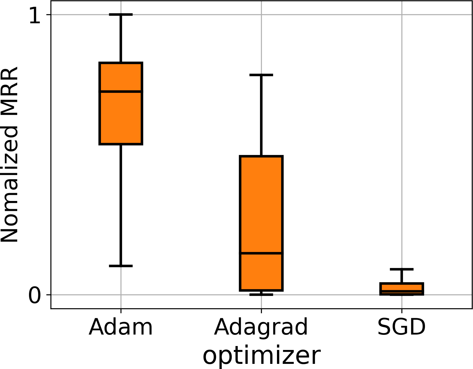
(a) optimizer

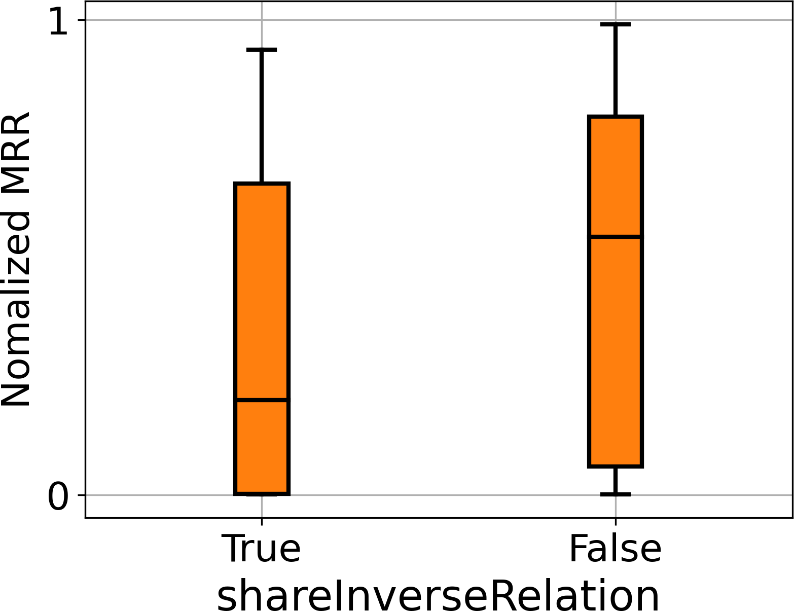
(b) add inverse relation

Figure 10: HPs that have fixed choice since one configure has significant advantage.

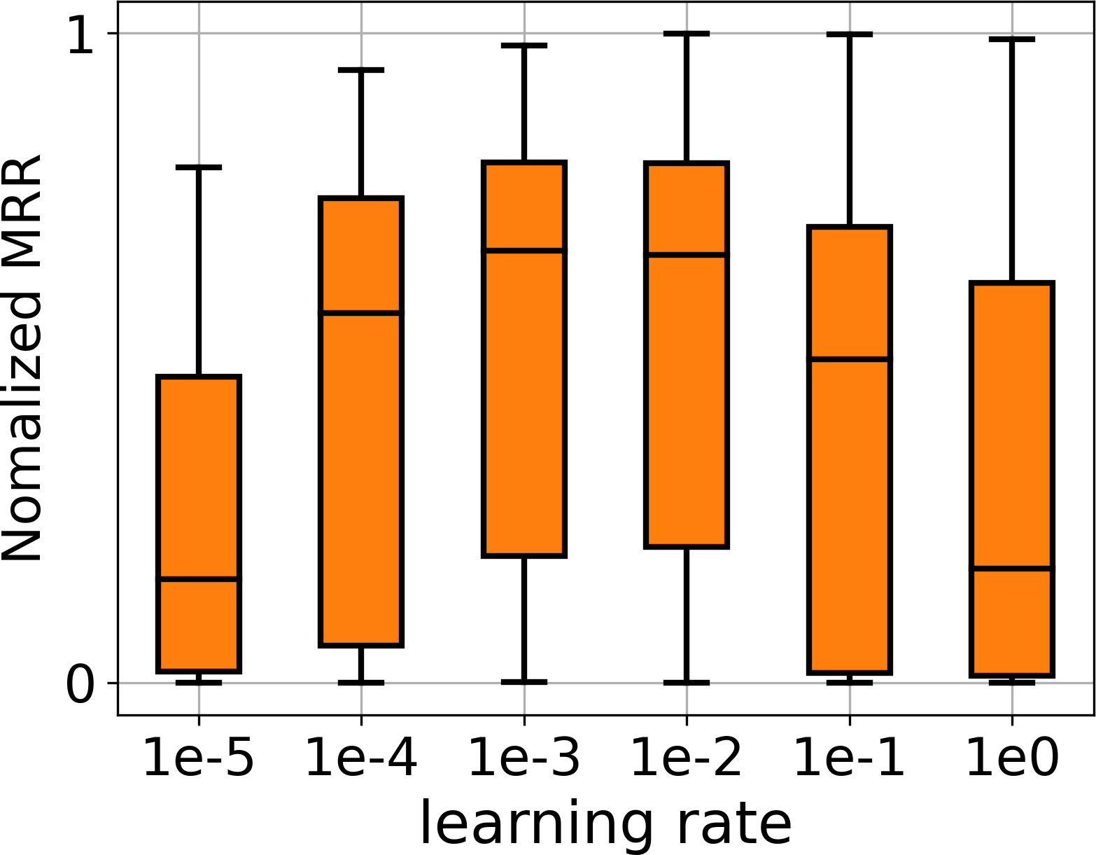
(a) learning rate

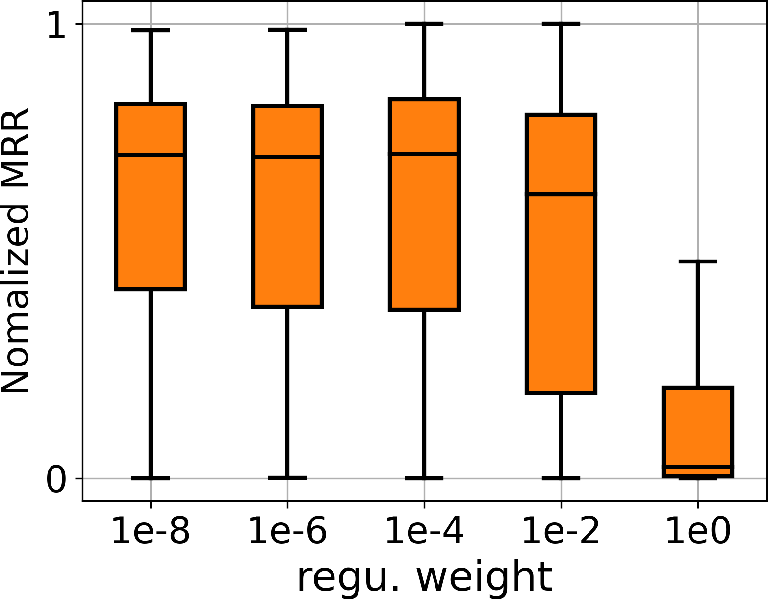
(b) reg. weight

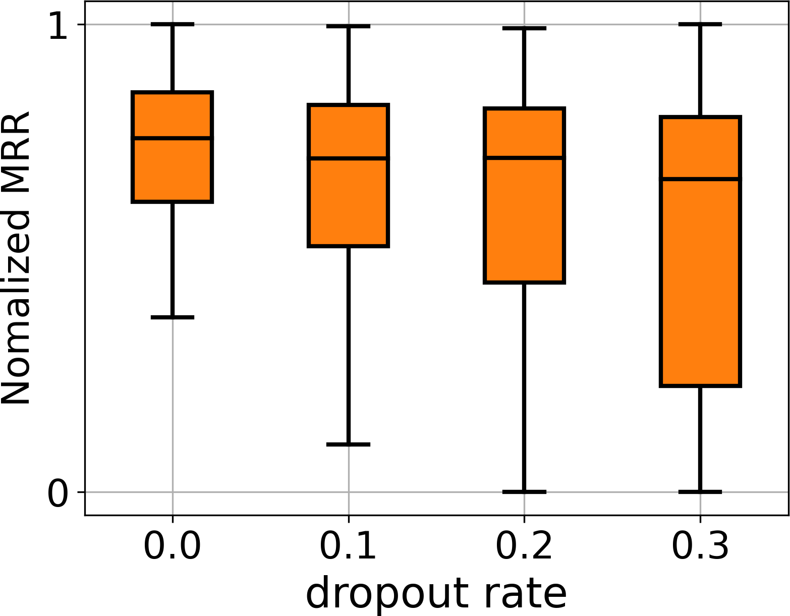
(c) dropout rate

Figure 11: HPs that have limited ranges since they only perform well in certain ranges.

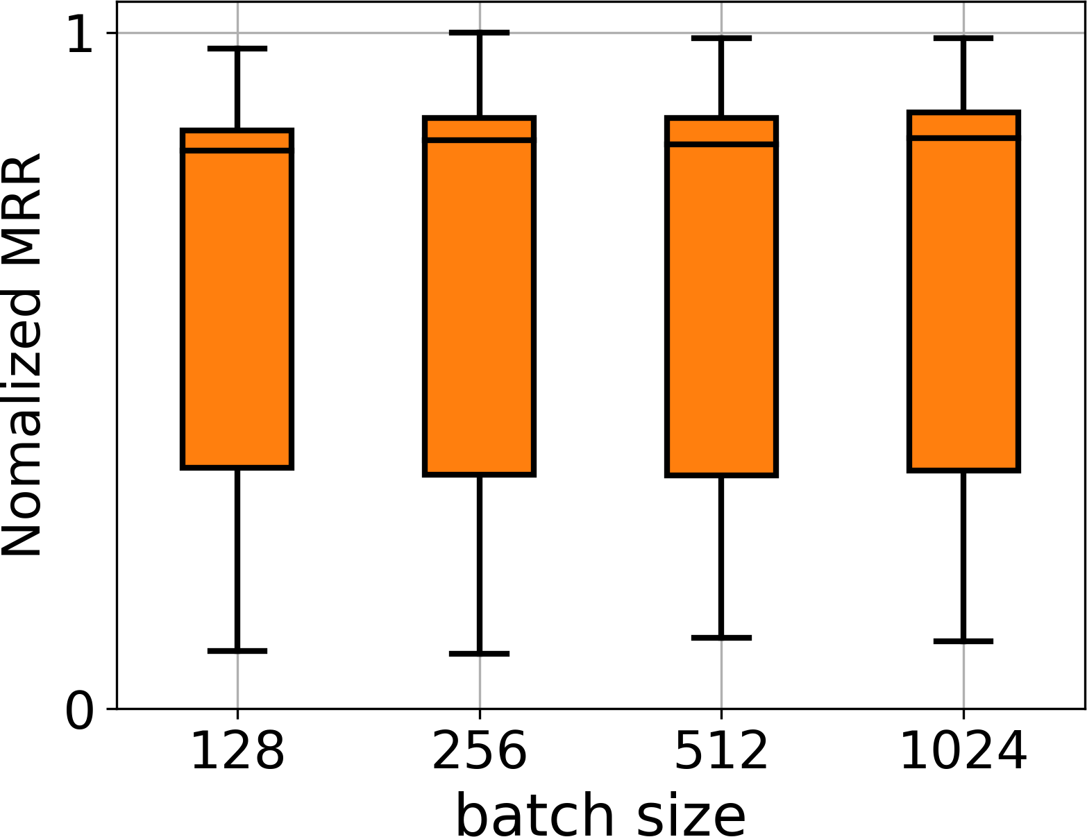
(a) batch_size

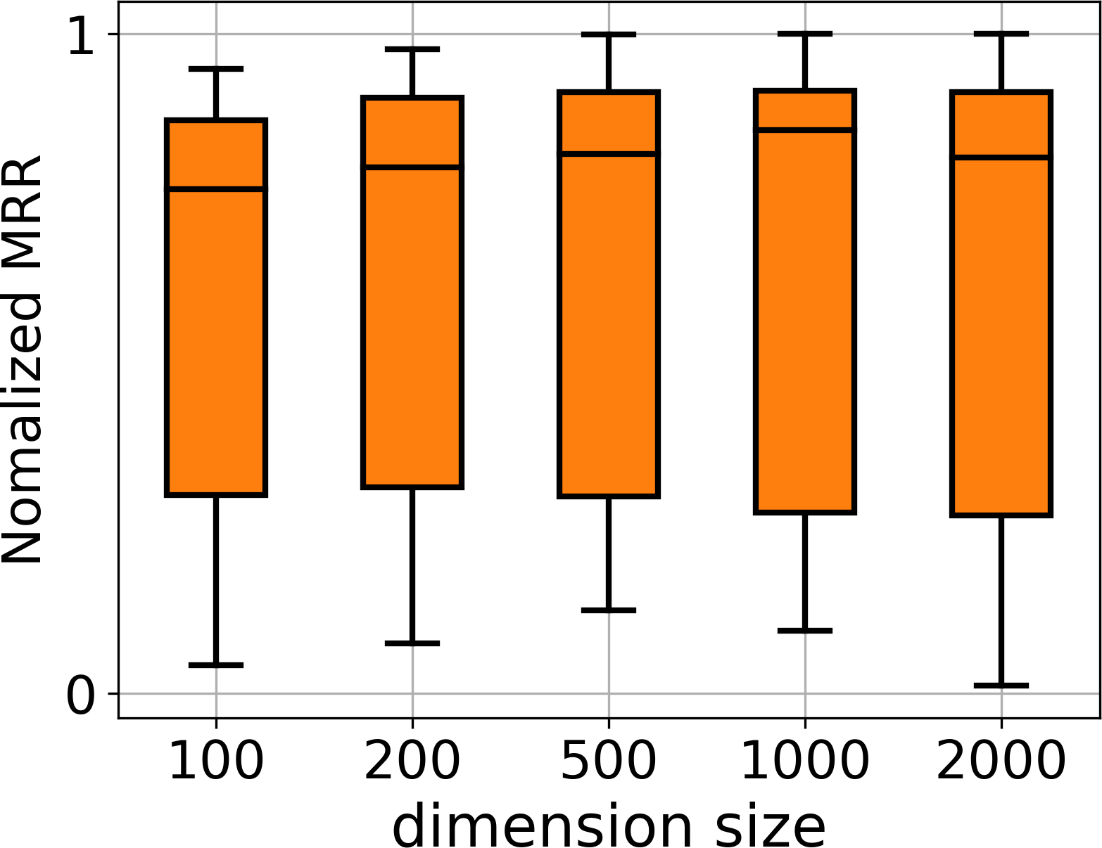
(b) dimension

Figure 12: HPs that is monotonic with different choices of values.

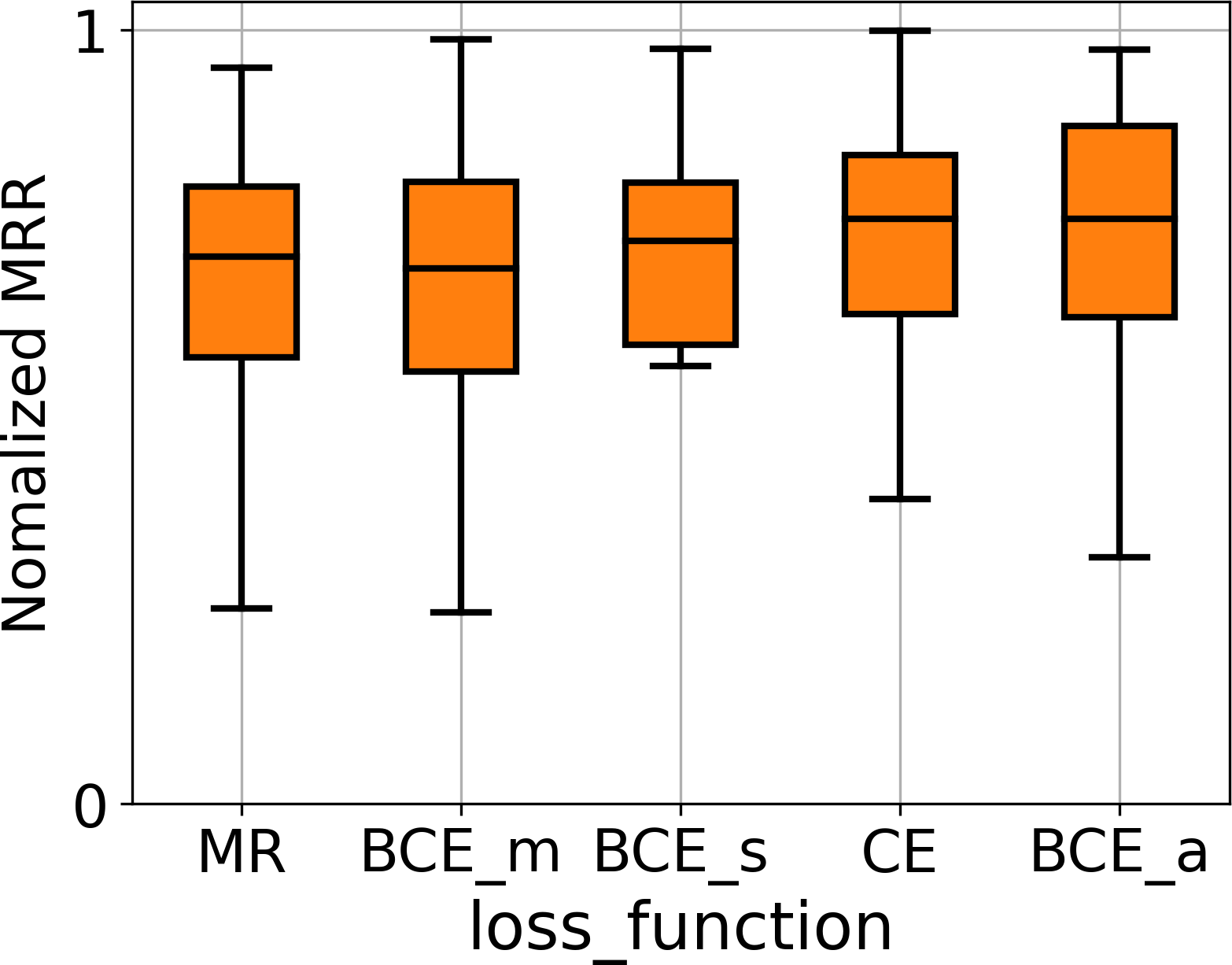
(a) loss

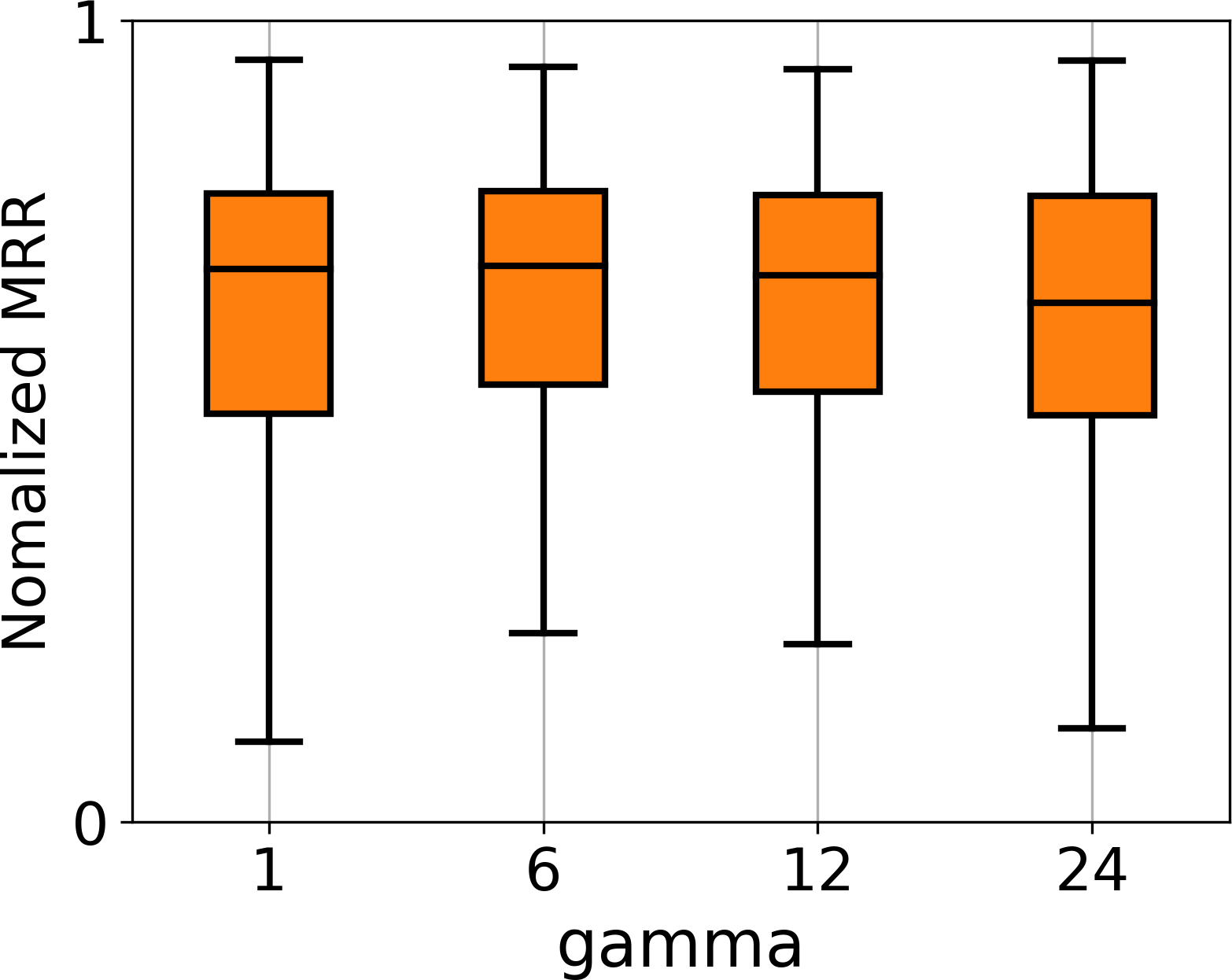
(b) gamma (MR)

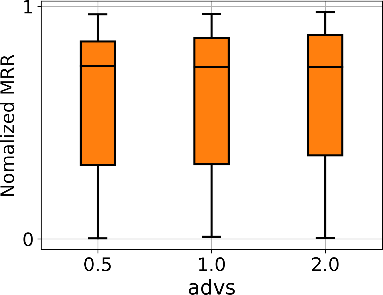
(c) adv weight (BCE_adv)

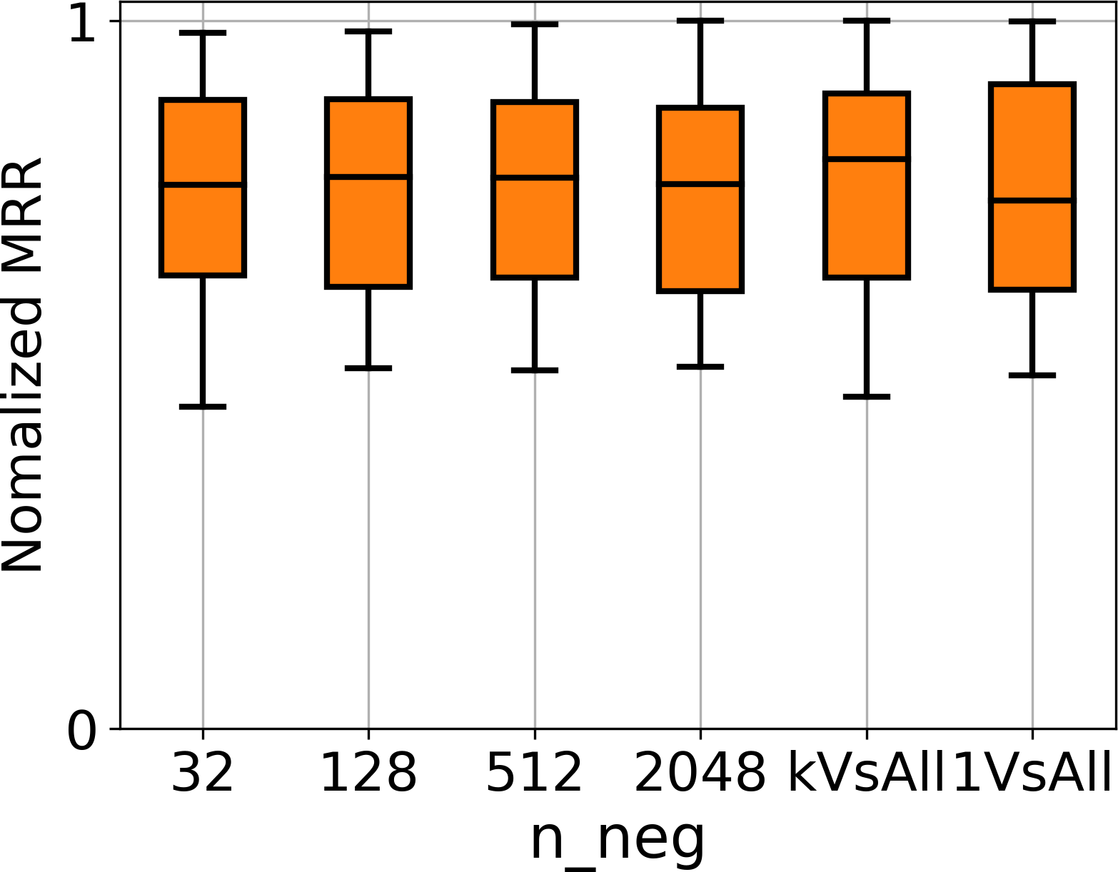
(d) # negative sample

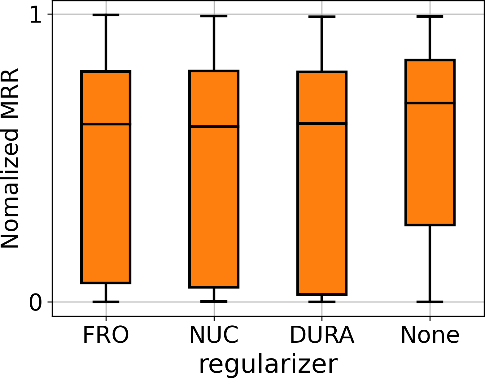
(e) regularizer

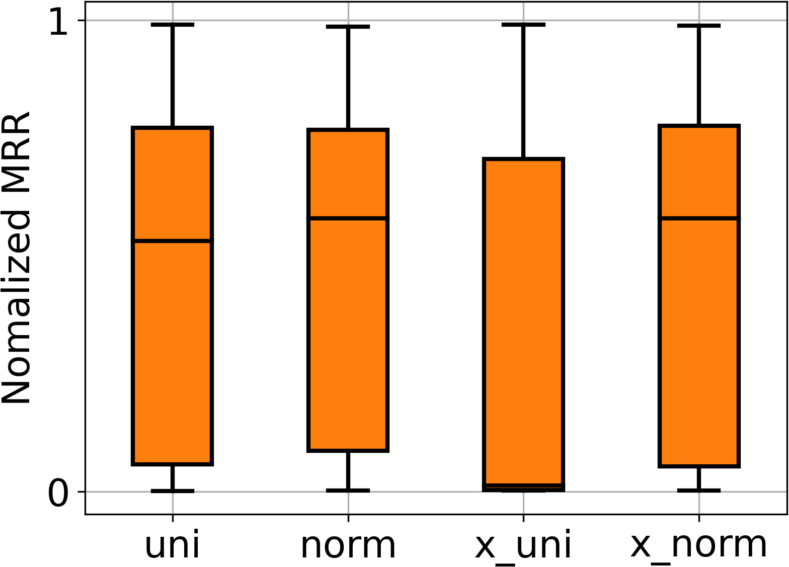
(f) initializer

Figure 13: HPs that do not have obvious patterns. All of the values should be searched.

B.3 Approximation ability of surrogate models

In Section 4.2, we have shown that the curvature of a learned random forest (RF) model is more similar with the real curvature of the ground truth. Here, we further demonstrate this point through a synthetic experiment.

Specifically, 100 random configurations with evaluated performance are sampled. We use 10/20/30 random samples from them to train the surrogates since only a small number of HP configurations are available for the surrogate during searching. The remaining configurations are used for testing. Then, we evaluate the fitting ability of each model by the mean square error (MSE) of the estimated prediction to the target prediction. For GP (Rasmussen, 2003), we show the prediction with the Matern kernel used in AutoNE (Tu et al., 2019). For RF (Breiman, 2001), we build 200 tree estimators to fit the training samples. The MLP here (Gardner and Dorling, 1998) is designed as a three-layer feed-forward network with 100 hidden units and ReLU activation function in each layer. The average value and std of MSE over five different groups of configurations are shown in Table 7. As can been seen, random forest show much lower prediction error than GP and MLP with different number of training samples. This further demonstrates that RF can better fit such a complex HP search space.

Table 7: Comparison of different surrogate models in MSE.

# train configurations	10	20	30
GP	0.0693$\pm$0.02	0.029$\pm$0.01	0.019$\pm$0.01
MLP	2.121$\pm$0.4	2.052$\pm$0.3	0.584$\pm$0.1
RF	0.003$\pm$0.002	0.002$\pm$0.001	0.001$\pm$0.001

B.4 Results of cost evaluation

We show the average cost and standard derivation of five HPs, i.e. batch size, dimension size, number of negative samples, loss functions, and regularizer, in Figure 14. As can be seen, the cost of batch size and dimension size increase much when the size increases. But for the number of negative samples, choices of loss functions and regularizers, the influence on cost is not strong as indicated by the average cost.

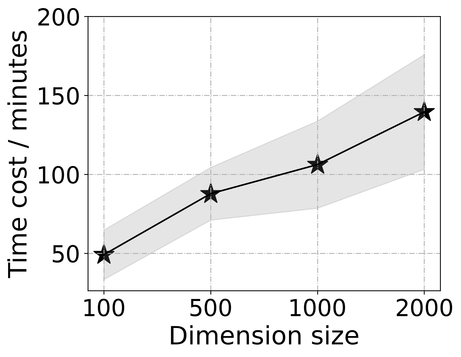
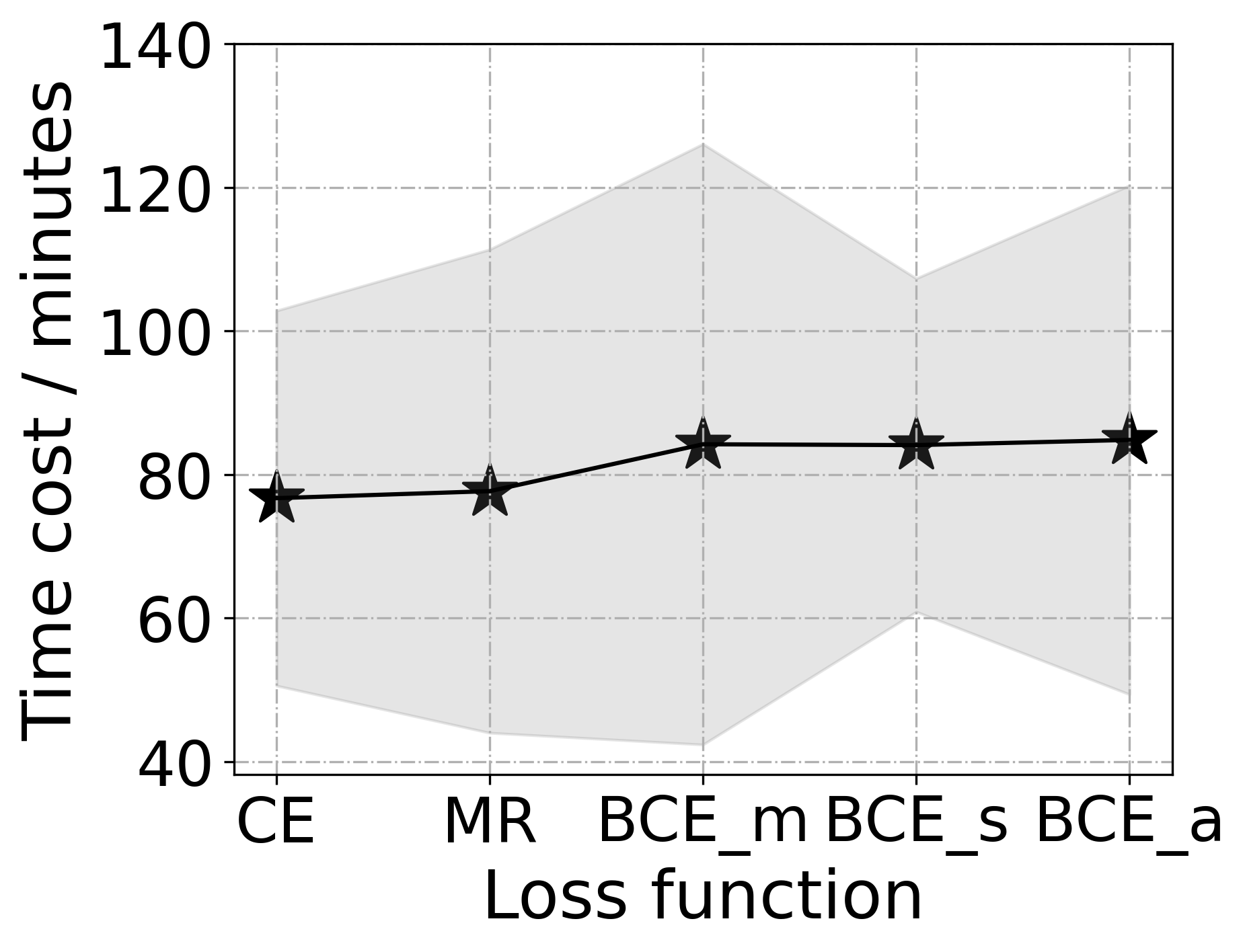
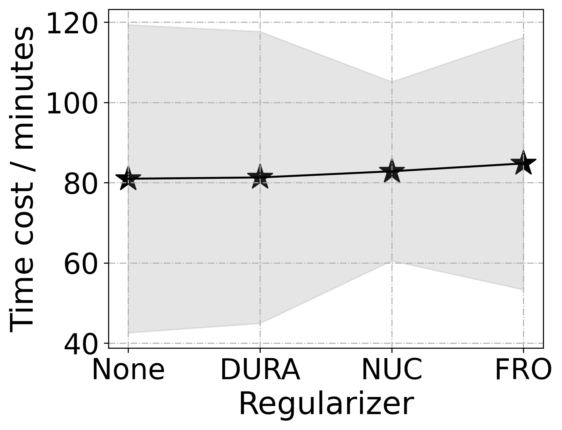
Figure 14: Computing time cost. The dots are the average and the shades are the standard deviation.

Appendix C Detail for the search algorithm

C.1 Search space

We show the shrunken and decoupled search space compared with the full space in Table 8. To evaluate the ratio of space change after shrinkage and decoupling, we measure the learning rate and regularization weight in log scale. The size of the whole space $\mathcal{X}$ compared with the decoupled ${\mathcal{X}}_{S|D}$ is

$$3\times\frac{14}{6}\times\frac{5}{3}\times\frac{5}{3}\times 2\times 4\times 5=777.8.$$

Hence, the reduced and decoupled space is hundreds times smaller than the full space.

Table 8: The revised HP values in the reduced and decoupled search space compared with the full space.

name	ranges in the whole space	revised ranges
optimizer	{Adam, Adagrad, SGD}	Adam
learning rate	[$10^{-5}$, $10^{0}$]	[$10^{-4}$, $10^{-1}$]
reg. weight	[$10^{-12}$, $10^{2}$]	[$10^{-8}$, $10^{-2}$]
dropout rate	[0, 0.5]	[0, 0.3]
inverse relation	{True, False}	{False}
batch size	{128, 256, 512, 1024}	128
dimension size	{100, 200, 500, 1000, 2000}	100

C.2 Search algorithm

We visualize the searching process of the traditional one-stage method and the proposed two-stage method in Figure 15. Since the evaluation cost on the full graph is rather high, the one-stage method can only take a few optimization trials. Thus the search space remains unexplored for a large proportion, and the performance of the optimal configuration is hard to be guaranteed. As for the proposed two-stage method KGTuner, it efficiently explores the search space on the sampled subgraph at the first stage, and then fine-tunes the top-K configurations on the full graph.

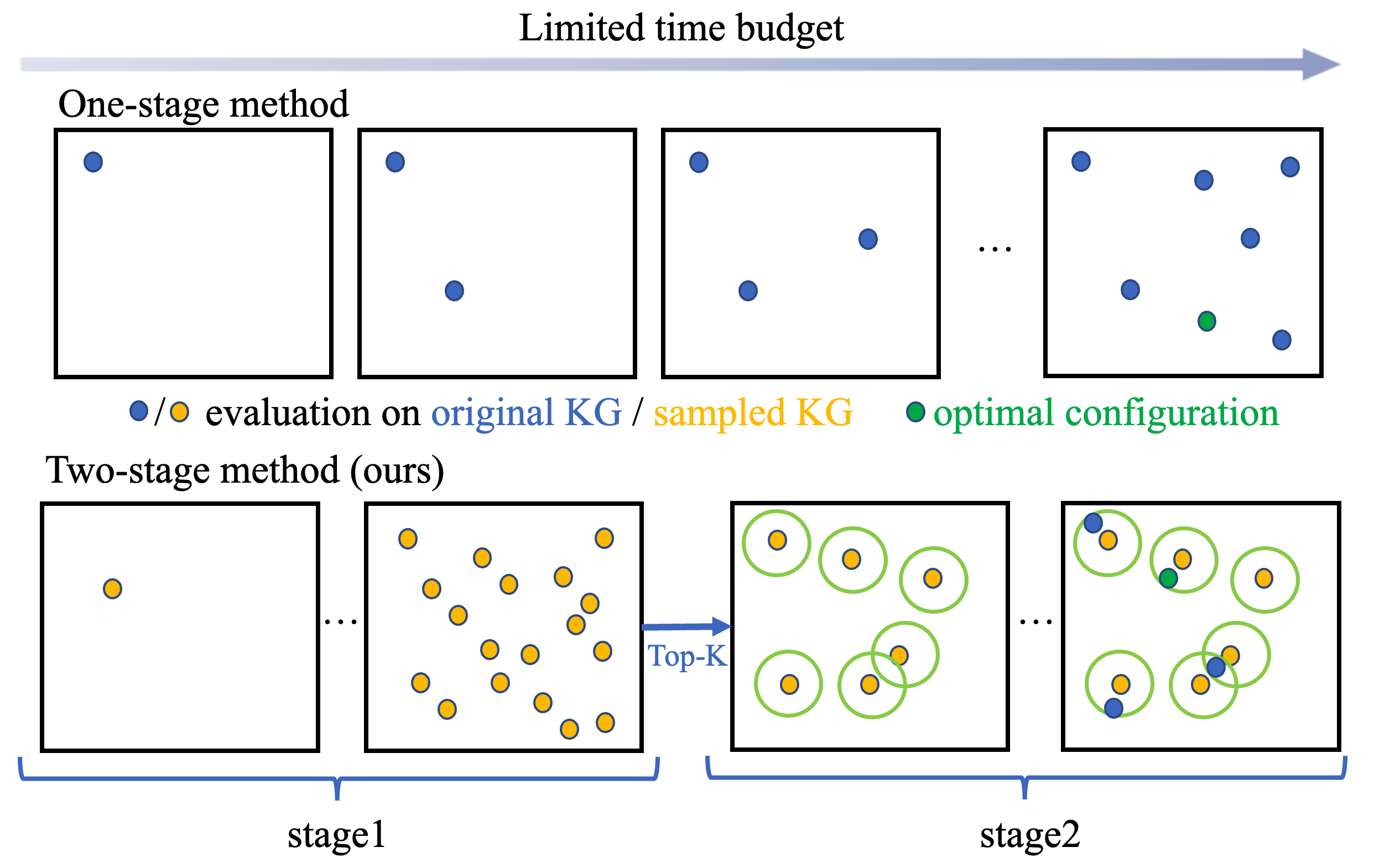
Figure 15: Diagram of one-stage search method and the proposed two-stage method.

In Algorithm 1, we increase the batch size and dimension size in stage two. We set the searched range for batch size in stage two as $[512,1024]$ and dimension size as $[1000,2000]$. There are some exceptions due to the memory issues, i.e., dimension size for RESCAL is in $[500,1000]$; dimension size for TuckER is in $[200,500]$. For ogbl-wikikg2, since the used GPU only has 24GB memory, we cannot run models with 500 dimensions which requires much more memory in the OGB board. Instead, we set the dimension as 100 to be consistent with the smaller models in OGB board with 100 dimensions, and increase the batch size in $[512,1024]$ in the second stage. In addition, we show the details for the search procedure by RF+BORE in Algorithm 2.

Algorithm 2 Full procedure of HP search with RF+BORE (in stage one)

0:  KG embedding $F$, dataset $G$, search space ${\mathcal{X}}_{S|D}$, budget $\nicefrac{{B}}{{2}}$, RF model $y=c(\mathbf{x})$, threshold $\tau=0.8$.

1:  initialize the RF model and $\mathcal{H}=\emptyset$;

2:  split triplets in $G$ with ratio $9:1$ into $G_{\text{tra}}$ and $G_{\text{val}}$;

3:  repeat

4:     randomly sample a set of configurations ${{\mathcal{X}}_{\overline{S|D}}}\subset{\mathcal{X}}_{S|D}$;

5:     select $\hat{\mathbf{x}}=\arg\max_{\mathbf{x}\in{{\mathcal{X}}_{\overline{S|D}}}}y(\mathbf{x})$;

6:     train embedding model into converge $\bm{P}^{*}=\arg\min_{\bm{P}}\mathcal{L}\big{(}F(\bm{P},\hat{\mathbf{x}}),G_{\text{tra}}\big{)}$;

7:     evaluate the performance $\hat{y}_{\hat{\mathbf{x}}}=\mathcal{M}\big{(}F(\bm{P}^{*},\hat{\mathbf{x}}),G_{\text{val}}\big{)}$;

8:     record $\mathcal{H}\leftarrow\mathcal{H}\cup\{(\hat{\mathbf{x}},\hat{y}_{\hat{\mathbf{x}}})\}$;% BORE:

9:     set label $0$ for configuration in $\mathcal{H}$ with $\hat{y}_{\hat{\mathbf{x}}}<\tau$, and label $1$ for $\hat{y}_{\hat{\mathbf{x}}}\geq\tau$;

10:     update RF model $y=c(\mathbf{x})$ to classify the two labels;

11:  until $\nicefrac{{B}}{{2}}$ exhausted.

Appendix D Additional experimental results

D.1 Implementation details

Evaluation metrics. We follow Bordes et al. (2013); Wang et al. (2017); Ruffinelli et al. (2019) to use the filtered ranking-based metrics for evaluation. For each triplet $(h,r,t)$ in the validation or testing set, we take the head prediction $(?,r,t)$ and tail prediction $(h,r,?)$ as the link prediction task. The filtered rankings on the head and tail are computed as

$$\text{rank}_{h}=\Big{|}\big{\{}e\in\mathcal{E}:\big{(}f(e,r,t)\geq f(h,r,t)\big{)}\wedge\big{(}(e,r,t)\notin D_{\text{tra}}\cup D_{\text{val}}\cup D_{\text{tst}})\big{)}\big{\}}\Big{|}+1,$$

$$\text{rank}_{t}=\Big{|}\big{\{}e\in\mathcal{E}:\big{(}f(h,r,t)\geq f(h,r,e)\big{)}\wedge\big{(}(h,r,e)\notin D_{\text{tra}}\cup D_{\text{val}}\cup D_{\text{tst}})\big{)}\big{\}}\Big{|}+1,$$

respectively, where $|\cdot|$ is the number of elements in the set. The the two metrics used are:

• Mean reciprocal ranking (MRR): the average of reciprocal of all the obtained rankings.

• Hit@$k$: the ratio of ranks no larger than $k$.

For both the metrics, the large value indicates the better performance.

Dataset statistics. We summarize the statistics of different benchmark datasets in Table 9. As shown, ogbl-biokg and ogbl-wikikg2 have much larger size compared with WN18RR and FB15k-237.

Table 9: Statistics of the KG completion datasets.

dataset	#entity	#relation	#train	#validate	#test
WN18RR  Dettmers et al. (2017)	41k	11	87k	3k	3k
FB15k-237 Toutanova and Chen (2015)	15k	237	272k	18k	20k
ogbl-biokg Hu et al. (2020)	94k	51	4,763k	163k	163k
ogbl-wikikg2 Hu et al. (2020)	2,500k	535	16,109k	429k	598k

Baseline implementation. All the baselines compared in this paper are based on their own original open-source implementations. Here we list the source links:

• Hyperopt (Bergstra et al., 2013), https://github.com/hyperopt/hyperopt;

• Ax, https://github.com/facebook/Ax;

• SMAC (Hutter et al., 2011), https://github.com/automl/SMAC3;

• BORE (Tiao et al., 2021), https://github.com/ltiao/bore;

• AutoNE (Tu et al., 2019), https://github.com/tadpole/AutoNE.

Searched hyperparameters. We list the searched hyperparameters for each embedding model on the different datasets in Tables 10-13 for reproduction.

Table 10: Searched optimal hyperparameters for the WN18RR dataset.

HP/Model	ComplEx	DistMult	RESCAL	ConvE	TransE	RotatE	TuckER
# negative samples	32	128	128	512	128	2048	128
loss function	BCE_mean	BCE_adv	BCE_mean	BCE_adv	BCE_adv	BCE_adv	BCE_adv
gamma	2.29	12.88	2.41	12.16	3.50	3.78	12.97
adv. weight	0.00	1.41	0.00	0.78	1.14	1.66	1.94
regularizer	NUC	NUC	DURA	DURA	FRO	FRO	DURA
reg. weight	$1.21\times 10^{-3}$	$9.58\times 10^{-3}$	$1.76\times 10^{-3}$	$9.79\times 10^{-3}$	$4.19\times 10^{-4}$	$5.13\times 10^{-8}$	$2.22\times 10^{-3}$
dropout rate	0.28	0.29	0.00	0.02	0.00	0.00	0.00
optimizer	Adam	Adam	Adam	Adam	Adam	Adam	Adam
learning rate	$6.08\times 10^{-4}$	$4.58\times 10^{-3}$	$1.73\times 10^{-3}$	$6.88\times 10^{-4}$	$1.02\times 10^{-4}$	$1.24\times 10^{-3}$	$2.60\times 10^{-3}$
initializer	x_uni	norm	uni	x_uni	norm	norm	x_uni
batch size	1024	1024	512	512	512	512	512
dimension size	2000	2000	1000	1000	1000	1000	200
inverse relation	False	False	False	False	False	False	False

Table 11: Searched optimal hyperparameters for the FB15k-237 dataset.

HP/Model	ComplEx	DistMult	RESCAL	ConvE	TransE	RotatE	TuckER
# negative samples	512	kVsAll	2048	512	512	128	2048
loss function	BCE_adv	CE	CE	BCE_sum	BCE_adv	BCE_adv	BCE_adv
gamma	13.05	2.90	4.17	14.52	6.76	14.46	13.51
adv. weight	1.93	0.00	0.00	0.00	1.99	1.12	1.95
regularizer	DURA	NUC	DURA	DURA	FRO	NUC	DURA
reg. weight	$9.75\times 10^{-3}$	$2.13\times 10^{-3}$	$8.34\times 10^{-3}$	$6.42\times 10^{-3}$	$2.16\times 10^{-4}$	$2.99\times 10^{-4}$	$2.66\times 10^{-4}$
dropout rate	0.22	0.29	0.01	0.07	0.02	0.01	0.01
optimizer	Adam	Adam	Adam	Adam	Adam	Adam	Adam
learning rate	$9.70\times 10^{-4}$	$4.91\times 10^{-4}$	$9.30\times 10^{-4}$	$2.09\times 10^{-4}$	$2.66\times 10^{-4}$	$5.89\times 10^{-4}$	$3.35\times 10^{-4}$
initializer	uni	x_uni	x_uni	norm	x_norm	norm	norm
batch size	1024	1024	2048	1024	512	1024	1024
dimension size	2000	1000	500	500	1000	2000	500
inverse relation	False	False	False	False	False	False	False

Table 12: Searched optimal hyperparameters for the ogbl-biokg dataset.

HP/Model	ComplEx	DistMult	TransE	RotatE	AutoSF
# negative samples	512	512	128	128	512
loss function	CE	CE	CE	BCE_adv	CE
gamma	12.90	11.82	7.60	18.34	12.90
adv. weight	0.00	0.00	0.00	1.94	0.00
regularizer	NUC	NUC	NUC	DURA	NUC
reg. weight	$1.38\times 10^{-3}$	$1.20\times 10^{-6}$	$6.99\times 10^{-3}$	$1.09\times 10^{-6}$	$1.38\times 10^{-4}$
dropout rate	0.01	0.00	0.00	0.00	0.01
optimizer	Adam	Adam	Adam	Adam	Adam
learning rate	$1.89\times 10^{-3}$	$1.25\times 10^{-3}$	$1.24\times 10^{-4}$	$1.11\times 10^{-4}$	$1.89\times 10^{-3}$
initializer	uni	x_uni	x_uni	norm	uni
batch size	1024	1024	1024	1024	1024
dimension size	2000	1000	2000	2000	2000
inverse relation	False	False	False	False	False

Table 13: Searched optimal hyperparameters for the ogbl-wikikg2 dataset

HP/Model	ComplEx	DistMult	TransE	RotatE	AutoSF
# negative samples	32	32	128	32	2048
loss function	CE	CE	CE	CE	CE
gamma	6.00	6.00	21.05	23.94	18.91
adv. weight	0.00	0.00	0.00	0.00	0.00
regularizer	DURA	DURA	FRO	DURA	DURA
reg. weight	$9.58\times 10^{-7}$	$1.98\times 10^{-4}$	$1.56\times 10^{-5}$	$8.10\times 10^{-3}$	$1.38\times 10^{-4}$
dropout rate	0.00	0.00	0.01	0.07	0.07
optimizer	Adam	Adam	Adam	Adam	Adam
learning rate	$1.34\times 10^{-4}$	$1.98\times 10^{-4}$	$6.05\times 10^{-4}$	$4.07\times 10^{-2}$	$1.04\times 10^{-2}$
initializer	x_norm	x_norm	x_norm	x_norm	x_norm
batch size	1024	1024	1024	1024	1024
dimension size	100	100	100	100	100
inverse relation	False	False	False	False	False

D.2 Results on general benchmarks

We compare the types of results on WN18RR and FB15k-237 in Table 14. In the first part, we show the results reported in the original papers. In the second part, we show the reproduced results in (Ruffinelli et al., 2019). And in the third part, we show the results of the HPs searched by KGTuner.

Table 14: Performance on WN18RR and FB15k-237 dataset. The bold numbers mean the best performances of the same model, and the underlines mean the second best.

		WN18RR				FB15k-237
		MRR	Hit@1	Hit@3	Hit@10	MRR	Hit@1	Hit@3	Hit@10
Original	ComplEx	0.440	0.410	0.460	0.510	0.247	0.158	0.275	0.428
	DistMult	0.430	0.390	0.440	0.490	0.241	0.155	0.263	0.419
	RESCAL	0.420	-	-	0.447	0.270	-	-	0.427
	ConvE	0.430	0.400	0.440	0.520	0.325	0.237	0.356	0.501
	TransE	0.226	-	-	0.501	0.294	-	-	0.465
	RotatE	0.476	0.428	0.492	0.571	0.338	0.241	0.375	0.533
	TuckER	0.470	0.443	0.482	0.526	0.358	0.266	0.394	0.544
LibKGE (Ruffinelli et al., 2019)	ComplEx	0.475	0.438	0.490	0.547	0.348	0.253	0.384	0.536
	DistMult	0.452	0.413	0.466	0.530	0.343	0.250	0.378	0.531
	RESCAL	0.467	0.439	0.480	0.517	0.356	0.263	0.393	0.541
	ConvE	0.442	0.411	0.451	0.504	0.339	0.248	0.369	0.521
	TransE	0.228	0.053	0.368	0.520	0.313	0.221	0.347	0.497
KGTuner (ours)	ComplEx	0.484	0.440	0.506	0.562	0.352	0.263	0.387	0.530
	DistMult	0.453	0.407	0.468	0.548	0.345	0.254	0.377	0.527
	RESCAL	0.479	0.436	0.496	0.557	0.357	0.268	0.390	0.535
	ConvE	0.437	0.399	0.449	0.515	0.335	0.242	0.368	0.523
	TransE	0.233	0.032	0.399	0.542	0.327	0.228	0.369	0.522
	RotatE	0.480	0.427	0.501	0.582	0.338	0.243	0.373	0.527
	TuckER	0.480	0.437	0.500	0.557	0.347	0.255	0.382	0.534

D.3 Full results for OGB

Table 15: Full results on ogbl-biokg and ogbl-wikikg2 dataset.

		ogbl-biokg			ogbl-wikikg2
		Test MRR	Val MRR	#parameters	Test MRR	Val MRR	#parameters
	ComplEx	0.8095$\pm$0.0007	0.8105$\pm$0.0001	187,648,000	0.4027$\pm$0.0027	0.3759$\pm$0.0016	1,250,569,500
OGB	DistMult	0.8043$\pm$0.0003	0.8055$\pm$0.0003	187,648,000	0.3729$\pm$0.0045	0.3506$\pm$0.0042	1,250,569,500
board	RotatE	0.7989$\pm$0.0004	0.7997$\pm$0.0002	187,597,000	0.2530$\pm$0.0034	0.2250$\pm$0.0035	250,087,150
	TransE	0.7452$\pm$0.0004	0.7456$\pm$0.0003	187,648,000	0.4256$\pm$0.0030	0.4272$\pm$0.0030	1,250,569,500
	AutoSF	0.8309$\pm$0.0008	0.8317$\pm$0.0007	187,648,000	0.5186$\pm$0.0065	0.5239$\pm$0.0074	250,113,900
KGTuner	ComplEx	0.8385$\pm$0.0009	0.8394$\pm$0.0007	187,648,000	0.4942$\pm$0.0017	0.5099$\pm$0.0023	250,113,900
	DistMult	0.8241$\pm$0.0008	0.8245$\pm$0.0009	93,824,000	0.4837$\pm$0.0078	0.5004$\pm$0.0075	250,113,900
	RotatE	0.8013$\pm$0.0015	0.8024$\pm$0.0012	187,597,000	0.2948$\pm$0.0026	0.2650$\pm$0.0034	250,087,150
	TransE	0.7781$\pm$0.0009	0.7787$\pm$0.0008	187,648,000	0.4739$\pm$0.0021	0.4932$\pm$0.0013	250,113,900
	AutoSF	0.8354$\pm$0.0013	0.8361$\pm$0.0012	187,648,000	0.5222$\pm$0.0021	0.5397$\pm$0.0023	250,113,900

References

- Ali et al. (2020) Mehdi Ali, Max Berrendorf, Charles Tapley Hoyt, Laurent Vermue, Mikhail Galkin, Sahand Sharifzadeh, Asja Fischer, Volker Tresp, and Jens Lehmann. 2020. Bringing light into the dark: A large-scale evaluation of knowledge graph embedding models under a unified framework. Technical report, arXiv:2006.13365.
- Balažević et al. (2019) Ivana Balažević, Carl Allen, and Timothy M Hospedales. 2019. Tucker: Tensor factorization for knowledge graph completion. In EMNLP.
- Bergstra et al. (2011) James Bergstra, Rémi Bardenet, Yoshua Bengio, and Balázs Kégl. 2011. Algorithms for hyper-parameter optimization. In NIPS, pages 2546–2554.
- Bergstra and Bengio (2012) James Bergstra and Yoshua Bengio. 2012. Random search for hyper-parameter optimization. JMLR, 13(2).
- Bergstra et al. (2013) James Bergstra, Dan Yamins, David D Cox, et al. 2013. Hyperopt: A python library for optimizing the hyperparameters of machine learning algorithms. In Proceedings of the 12th Python in science conference, volume 13, page 20. Citeseer.
- Bordes et al. (2014) Antoine Bordes, Sumit Chopra, and Jason Weston. 2014. Question answering with subgraph embeddings. In EMNLP.
- Bordes et al. (2013) Antoine Bordes, Nicolas Usunier, Alberto Garcia-Duran, Jason Weston, and Oksana Yakhnenko. 2013. Translating embeddings for modeling multi-relational data. In NeurIPS, pages 2787–2795.
- Breiman (2001) Leo Breiman. 2001. Random forests. ML, 45(1):5–32.
- Cai and Wang (2018) Liwei Cai and William Yang Wang. 2018. Kbgan: Adversarial learning for knowledge graph embeddings. In NAACL, pages 1470–1480.
- Claesen and De Moor (2015) Marc Claesen and Bart De Moor. 2015. Hyperparameter search in machine learning. Technical report, arXiv:1502.02127.
- Colson et al. (2007) Benoît Colson, Patrice Marcotte, and Gilles Savard. 2007. An overview of bilevel optimization. Ann. Oper. Res., 153(1):235–256.
- Dettmers et al. (2017) Tim Dettmers, Pasquale Minervini, Pontus Stenetorp, and Sebastian Riedel. 2017. Convolutional 2D knowledge graph embeddings. In AAAI.
- Duchi et al. (2011) John Duchi, Elad Hazan, and Yoram Singer. 2011. Adaptive subgradient methods for online learning and stochastic optimization. JMLR, 12(7).
- Fawcett and Hoos (2016) Chris Fawcett and Holger H Hoos. 2016. Analysing differences between algorithm configurations through ablation. Journal of Heuristics, 22(4):431–458.
- Gardner and Dorling (1998) Matt W Gardner and SR Dorling. 1998. Artificial neural networks (the multilayer perceptron) – a review of applications in the atmospheric sciences. Atmospheric environment, 32(14-15):2627–2636.
- Goodfellow et al. (2016) Ian Goodfellow, Yoshua Bengio, and Aaron Courville. 2016. Deep learning. MIT press.
- Guo et al. (2019) Lingbing Guo, Zequn Sun, and Wei Hu. 2019. Learning to exploit long-term relational dependencies in knowledge graphs. In ICML, pages 2505–2514.
- Hamilton et al. (2017) William L Hamilton, Rex Ying, and Jure Leskovec. 2017. Inductive representation learning on large graphs. In NIPS, pages 1025–1035.
- Hu et al. (2020) Weihua Hu, Matthias Fey, Marinka Zitnik, Yuxiao Dong, Hongyu Ren, Bowen Liu, Michele Catasta, and Jure Leskovec. 2020. Open graph benchmark: Datasets for machine learning on graphs. NeurIPS.
- Hutter et al. (2014) Frank Hutter, Holger Hoos, and Kevin Leyton-Brown. 2014. An efficient approach for assessing hyperparameter importance. In ICML, pages 754–762. PMLR.
- Hutter et al. (2011) Frank Hutter, Holger H Hoos, and Kevin Leyton-Brown. 2011. Sequential model-based optimization for general algorithm configuration. In ICLIO, pages 507–523. Springer.
- Ji et al. (2021) Shaoxiong Ji, Shirui Pan, Erik Cambria, Pekka Marttinen, and S Yu Philip. 2021. A survey on knowledge graphs: Representation, acquisition and applications. TNNLS.
- Kazemi and Poole (2018) Seyed Mehran Kazemi and David Poole. 2018. SimplE embedding for link prediction in knowledge graphs. In NeurIPS.
- Kingma and Ba (2014) Diederik P Kingma and Jimmy Ba. 2014. Adam: A method for stochastic optimization. In ICLR.
- Lacroix et al. (2018) Timothée Lacroix, Nicolas Usunier, and Guillaume Obozinski. 2018. Canonical tensor decomposition for knowledge base completion. In ICML, pages 2863–2872. PMLR.
- Leskovec and Faloutsos (2006) Jure Leskovec and Christos Faloutsos. 2006. Sampling from large graphs. In SIGKDD, pages 631–636.
- Li et al. (2017) Hao Li, Zheng Xu, Gavin Taylor, Christoph Studer, and Tom Goldstein. 2017. Visualizing the loss landscape of neural nets. In NIPS.
- Nickel et al. (2011) Maximilian Nickel, Volker Tresp, and Hans-Peter Kriegel. 2011. A three-way model for collective learning on multi-relational data. In ICML, volume 11, pages 809–816.
- Paszke et al. (2017) Adam Paszke, Sam Gross, Soumith Chintala, Gregory Chanan, Edward Yang, Zachary DeVito, Zeming Lin, Alban Desmaison, Luca Antiga, and Adam Lerer. 2017. Automatic differentiation in pytorch.
- Probst et al. (2019) Philipp Probst, Anne-Laure Boulesteix, and Bernd Bischl. 2019. Tunability: importance of hyperparameters of machine learning algorithms. JMLR, 20(1):1934–1965.
- Rasmussen (2003) Carl Edward Rasmussen. 2003. Gaussian processes in machine learning. In Summer school on machine learning, pages 63–71. Springer.
- Rossi et al. (2021) Andrea Rossi, Denilson Barbosa, Donatella Firmani, Antonio Matinata, and Paolo Merialdo. 2021. Knowledge graph embedding for link prediction: A comparative analysis. TKDD.
- Ruffinelli et al. (2019) Daniel Ruffinelli, Samuel Broscheit, and Rainer Gemulla. 2019. You can teach an old dog new tricks! on training knowledge graph embeddings. In ICLR.
- Saxena et al. (2020) Apoorv Saxena, Aditay Tripathi, and Partha Talukdar. 2020. Improving multi-hop question answering over knowledge graphs using knowledge base embeddings. In ACL, pages 4498–4507.
- Schlichtkrull et al. (2018) Michael Schlichtkrull, Thomas N Kipf, Peter Bloem, Rianne Van Den Berg, Ivan Titov, and Max Welling. 2018. Modeling relational data with graph convolutional networks. In ESWC, pages 593–607. Springer.
- Schober et al. (2018) Patrick Schober, Christa Boer, and Lothar A Schwarte. 2018. Correlation coefficients: appropriate use and interpretation. Anesthesia & Analgesia, 126(5):1763–1768.
- Snoek et al. (2012) Jasper Snoek, Hugo Larochelle, and Ryan P Adams. 2012. Practical bayesian optimization of machine learning algorithms. NIPS, 25.
- Sun et al. (2019) Zhiqing Sun, Zhi-Hong Deng, Jian-Yun Nie, and Jian Tang. 2019. Rotate: Knowledge graph embedding by relational rotation in complex space. In ICLR.
- Sun et al. (2020) Zhiqing Sun, Shikhar Vashishth, Soumya Sanyal, Partha Talukdar, and Yiming Yang. 2020. A re-evaluation of knowledge graph completion methods. In ACL, pages 5516–5522.
- Teru et al. (2020) Komal Teru, Etienne Denis, and Will Hamilton. 2020. Inductive relation prediction by subgraph reasoning. In ICML, pages 9448–9457. PMLR.
- Tiao et al. (2021) Louis C Tiao, Aaron Klein, Matthias Seeger, Edwin V Bonilla, Cedric Archambeau, and Fabio Ramos. 2021. Bore: Bayesian optimization by density-ratio estimation. In ICML.
- Toutanova and Chen (2015) Kristina Toutanova and Danqi Chen. 2015. Observed versus latent features for knowledge base and text inference. In ACL Workshop, pages 57–66.
- Trouillon et al. (2017) Théo Trouillon, Christopher R Dance, Johannes Welbl, Sebastian Riedel, Éric Gaussier, and Guillaume Bouchard. 2017. Knowledge graph completion via complex tensor factorization. JMLR, 18(1):4735–4772.
- Tu et al. (2019) Ke Tu, Jianxin Ma, Peng Cui, Jian Pei, and Wenwu Zhu. 2019. AutoNE: Hyperparameter optimization for massive network embedding. In SIGKDD, pages 216–225.
- Vashishth et al. (2020) Shikhar Vashishth, Soumya Sanyal, Vikram Nitin, and Partha Talukdar. 2020. Composition-based multi-relational graph convolutional networks. ICLR.
- Wang et al. (2017) Quan Wang, Zhendong Mao, Bin Wang, and Li Guo. 2017. Knowledge graph embedding: A survey of approaches and applications. TKDE, 29(12):2724–2743.
- Wang et al. (2021) Xin Wang, Shuyi Fan, Kun Kuang, and Wenwu Zhu. 2021. Explainable automated graph representation learning with hyperparameter importance. In ICML, pages 10727–10737. PMLR.
- Wang et al. (2018) Yanjie Wang, Rainer Gemulla, and Hui Li. 2018. On multi-relational link prediction with bilinear models. In AAAI.
- Williams and Rasmussen (1995) Christopher KI Williams and Carl Edward Rasmussen. 1995. Gaussian processes for regression. In NIPS, pages 514–520.
- Yang et al. (2015) Bishan Yang, Wen-tau Yih, Xiaodong He, Jianfeng Gao, and Li Deng. 2015. Embedding entities and relations for learning and inference in knowledge bases. In ICLR.
- You et al. (2020) Jiaxuan You, Zhitao Ying, and Jure Leskovec. 2020. Design space for graph neural networks. NeurIPS, 33.
- Zhang et al. (2016) Fuzheng Zhang, Nicholas Jing Yuan, Defu Lian, Xing Xie, and Wei-Ying Ma. 2016. Collaborative knowledge base embedding for recommender systems. In SIGKDD, pages 353–362.
- Zhang and Yao (2022) Yongqi Zhang and Quanming Yao. 2022. Knowledge graph reasoning with relational digraph. Technical report, arXiv:2108.06040.
- Zhang et al. (2021) Yongqi Zhang, Quanming Yao, and Lei Chen. 2021. Simple and automated negative sampling for knowledge graph embedding. VLDB-J, 30(2):259–285.
- Zhang et al. (2020a) Yongqi Zhang, Quanming Yao, Wenyuan Dai, and Lei Chen. 2020a. AutoSF: Searching scoring functions for knowledge graph embedding. In ICDE, pages 433–444.
- Zhang et al. (2020b) Zhanqiu Zhang, Jianyu Cai, and Jie Wang. 2020b. Duality-induced regularizer for tensor factorization based knowledge graph completion. NeurIPS, 33.