Gravitational-wave evolution of newborn magnetars with different deformed structures

Abstract

Weak and continuous gravitational-wave (GW) radiation can be produced by newborn magnetars with deformed structure and is expected to be detected by the Einstein telescope in the near future. In this work we assume that the deformed structure of a nascent magnetar is not caused by a single mechanism but by multiple time-varying quadrupole moments such as those present in magnetically induced deformation, starquake-induced ellipticity, and accretion column-induced deformation. The magnetar loses its angular momentum through accretion, magnetic dipole radiation, and GW radiation. Within this scenario, we calculate the evolution of GWs from a newborn magnetar by considering the above three deformations. We find that the GW evolution depends on the physical parameters of the magnetar (e.g., period and surface magnetic field), the adiabatic index, and the fraction of poloidal magnetic energy to the total magnetic energy. In general the GW radiation from a magnetically induced deformation is dominant if the surface magnetic field of the magnetar is large, but the GW radiation from magnetar starquakes is more efficient when there is a larger adiabatic index if all other magnetar parameters remain the same. We also find that the GW radiation is not very sensitive to different magnetar equations of state.

I introduction

Gravitational waves (GWs) are a prediction of the General Theory of Relativity. From a theoretical point of view, strong GW signals can be produced by cataclysmic events such as the merger of black holes (BHs), colliding neutron stars (NSs), as well as supernova explosions. In addition, weak GW signals are predicted to emanate from rotating NSs and are also predicted to be present in the Big Bang. In terms of observations, the first direct detection of GWs from a binary BH merger was the signal GW150914 observed by the Laser Interferometer Gravitational wave Observatory (LIGO; Ref [1]. Two years later, advanced LIGO and Virgo  [2, 3, 4, 5, 6, 7, 8] detected GW170817 from the merger of two neutron stars. Simultaneous to the GW170817 signal, electromagnetic signals emitted during this NS merger were detected, and the combined GW and EM signals opened the field of multimessenger astronomy to allow deeper exploration of the mysteries of the universe. However, the expected continuous GW signals emitted from isolated objects with asymmetric structures remain undetected thus far. These will be important scientific objects for next-generation GW detectors such as the Einstein telescope (ET).

Newborn millisecond magnetars are promising candidate sources of continuous GW radiation  [9, 10]. A direct search for postmerger GWs from the remnant of the binary NS merger GW170817 was performed by the aLIGO team  [11], but no GW signals were found. Reference [12] found indirect evidence of GW radiation in the afterglow of GRB 200219A, but the GW signal is too weak to be detected by aLIGO and Virgo.

To date, many deformation mechanisms that enable an isolated system to emit GWs have been proposed in the literature [13, 14, 15, 16, 17, 18, 19]. Magnetars are generally believed to have strong magnetic fields [20, 21, 22, 23, 24, 25, 26], and the magnetic stress is too large for the magnetar to maintain a long-lasting spherical structure [27]. Magnetars with large toroidal magnetic fields tend to become powerful GW emitters [28]. The dynamical simulations of Ref. [29] suggest that the NS crust is likely very strong and can support mountains large enough to produce GWs that can be detected in large-scale interferometers. The authors of Ref. [30] considered several examples for the form of the deforming force, and calculated that the maximum ellipticity that can support a neutron star crust is on the order of $10^{-8}-10^{-7}$. Afterwards, they applied it to the relativity case, and found that the maximum deformation that can support the crust of neutron star is two orders lower than the Newtonian case [31]. On the other hand, strong centrifugal forces in such magnetars can also break the NS’s crust to result in starquakes, and form an asymmetric structure of the star  [14]. Moreover, magnetars can be born in the core collapse of a massive star [32, 33, 34] or from the merger of binary stars [35, 36, 37, 38]. A fraction of the remnant material ejected in these processes does not reach the escape velocity and falls back. During the accretion process, the magnetic poles of magnetars with high accretion rates will form significant accretion columns [17]. Further studies were carried out in Ref. [39], and they take into account the time variables of magnetar parameters, such as accretion rate, spin period, magnetic field, and moments of inertia. The evolution of inclination angle is also considered in their study, which found that the magnetic axis is orthogonal to the axis of rotation immediately after the birth of the star, which causes the accretion column to produce time-varying quadrupoles and GW radiation [39]. In previous studies, several magnetar deformation mechanisms were even adopted to power the GW signals, but the authors did not consider simultaneously the contributions of all possible deformation mechanisms [13, 14, 15, 16, 17, 18, 19].

One basic problem is to describe the evolution of GW radiation if the three lines of deformation mechanisms, i.e. magnetically induced deformation, starquake-induced ellipticity, and an accretion mountain are considered simultaneously. Which magnetar deformation mechanism dominates the contribution to the GW radiation? In this paper, we study the evolution of GWs emitted from newborn magnetars by considering the three most likely deformations above. In Sec.II, we introduce briefly the theory of GW radiation production with the above three lines of deformation mechanisms one by one. The calculation of the GW evolution with the period and surface magnetic field of the magnetar, adiabatic index, the fraction of poloidal magnetic energy, and for different NS equations of state are shown in Sec.III. Conclusions are drawn in Sec.IV with some additional discussion.

II Deformation of the magnetar

In order to study the deformation of a magnetar, we first consider a background model of a spherical, nonmagnetic, nonrotating star. The hydrostatic equilibrium equation can be written as

$$\nabla p_{0}+\rho_{0}\nabla\phi_{0}=0,$$ (1)

where $p_{0}$ and $\rho_{0}$ are the initial pressure and density, respectively. The initial gravitational potential is $\phi_{0}$, and it obeys the Poisson equation:

$$\nabla^{2}\phi_{0}=4\pi G\rho_{0},$$ (2)

where $G$ is Newton’s gravitational constant. The density configuration can be given as described in Refs. [40, 41] by adopting the polytropic equation of state (EOS) with $n=1$ (e.g., $p=k\rho^{1+1/n}$):

$$\rho_{0}=\frac{M}{4rR^{2}}\sin\left(\frac{\pi r}{R}\right),$$ (3)

where $M$ and $R$ are the mass and radius of star, respectively.

Here, we consider a newborn magnetar with three asymmetric structures, i.e., magnetically induced deformation under strong magnetic stress, deformation due to a series of high spin-induced starquakes, and asymmetric accretion columns caused by fallback accretion. The density distribution $\rho$ will be affected by the asymmetric perturbation of the starquakes $\rho_{\mathrm{sta}}^{\Delta}$, magnetic stress $\rho_{\mathrm{mag}}^{\Delta}$, and accretion $\rho_{\mathrm{acc}}^{\Delta}$. Moreover, the density distribution is also disturbed $\rho_{\mathrm{cen}}$ by the centrifugal force . The density distribution $\rho(\bm{r})$ can therefore be represented as:

$$\rho(\bm{r})=\rho_{0}(r)+\rho_{\mathrm{cen}}(\bm{r})+\rho_{\mathrm{sta}}^{\Delta}(\bm{r})+\rho_{\mathrm{mag}}^{\Delta}(\bm{r})+\rho_{\mathrm{acc}}^{\Delta}(\bm{r}).$$ (4)

The GW radiation of a magnetar is very sensitive to the ellipticity ($\epsilon$), which is defined as

$$\epsilon=\frac{I_{yy}-I_{xx}}{I_{zz}}.$$ (5)

Furthermore, as long as the difference of $I_{yy}-I_{xx}$ is small, the contribution of perturbation can be neglected in $I_{zz}$ to calculate the $\epsilon$. Hence, we use the moment of inertia of the spherical star $I_{0}$ instead of $I_{zz}$ in our calculations. Here, we adopt $I_{jk}$ to denote the component of the inertia tensor $\mathbf{I}$:

$$\mathbf{I}=\int\rho(\bm{r})\left(r^{2}\hat{\mathbf{I}}-\bm{r}\otimes\bm{r}\right)dV,$$ (6)

where $\hat{\mathbf{I}}$ is unit tensor, and $\bm{r}\otimes\bm{r}$ is the dyadic product of $\bm{r}$. One can substitute Eq. (4) into Eq. (6) to calculate the ellipticity. We find that the initial density $\rho_{0}$ and the perturbation of the density by the centrifugal force $\rho_{\mathrm{cen}}$ would provide the same contributions to all the components of the inertia tensor as in the case of uniform rotation. The terms cancel out in calculating the ellipticity, i.e. $I_{yy}=I_{xx}$. Hence, the total ellipticity $\epsilon$ is only dependent on the asymmetric deformation due to the starquake $\epsilon_{\mathrm{sta}}$, magnetic field $\epsilon_{\mathrm{mag}}$, and accretion $\epsilon_{\mathrm{acc}}$ terms. It can be expressed as

$${\epsilon}= I_{0}^{-1}\int_{V}\left[\rho_{\mathrm{sta}}^{\Delta}(\bm{r})+\rho_{\mathrm{mag}}^{\Delta}(\bm{r})+\rho_{\mathrm{acc}}^{\Delta}(\bm{r})\right]\left(r_{x}^{2}-r_{y}^{2}\right)dV$$ (7)

$$=\epsilon_{\mathrm{sta}}+\epsilon_{\mathrm{mag}}+\epsilon_{\mathrm{acc}}.$$

The asymmetric density will give the star a nonzero ellipticity that results in the production of GW radiation when it is rotated at the appropriate angle, the luminosity of which can be expressed as

$$L_{\mathrm{gw}}=-\frac{2GI_{0}^{2}\Omega^{6}}{5c^{5}}\epsilon^{2}\sin^{2}\alpha(16\sin^{2}\alpha+\cos^{2}\alpha),$$ (8)

where $\Omega$ is angular frequency, $c$ is the speed of light, and $\alpha$ is the misalignment angle. In Ref. [39], the authors found that the magnetic and rotational axes of a star would be orthogonal in the early stages ($\leqslant 10$ ms), but gradually align after hundreds of years. These timescales are too short compared with the evolution time we are considering. Therefore, in our calculations we consider only the case that the magnetic axis ($z^{\prime}$) is perpendicular to the rotation axis ($z$). One can estimate the upper limit of the GW radiation luminosity of the magnetar with $\alpha=90^{\circ}$. Within this scenario, all three deformations we consider will be maximized at the equator and the GW radiation will reach its maximum efficiency.

II.1 Magnetically induced deformation

For convenience, a spherical coordinate system ($r$, ${\theta}^{\prime}$, ${\varphi}^{\prime}$) with the magnetic axis ${z}^{\prime}$ as the polar axis is used to calculate the deformation caused by the magnetic field. Based on Eq. (7), the magnetically induced ellipticity can be written as

$$\epsilon_{\mathrm{mag}}=I_{0}^{-1}\int_{V}\rho_{\mathrm{mag}}^{\Delta}(\bm{r})\left(r_{x}^{2}-r_{z^{\prime}}^{2}\right)dV.$$ (9)

Here, $\rho_{\mathrm{mag}}^{\Delta}$ is dependent on the configuration of the magnetic field. Let us adopt a universal configuration for the internal magnetic field with both poloidal $\bm{B}_{\mathrm{p}}=\left(B_{r},B_{\theta^{\prime}},0\right)$ and toroidal components $\bm{B}_{\mathrm{t}}=\left(0,0,B_{\phi^{\prime}}\right)$ which satisfy the requirement of a stable magnetic field [42]. One can adopt a stream function $S(r,\theta^{\prime})$ to express each component of the magnetic field [43]

$$B_{r}=\frac{B_{0}\eta_{p}\partial_{\theta^{\prime}}S}{2r^{2}\sin{\theta}^{\prime}},B_{\theta^{\prime}}=-\frac{B_{0}\eta_{p}\partial_{r}S}{2r\sin{\theta}^{\prime}},B_{\phi^{\prime}}=\frac{B_{0}\eta_{t}\beta(S)}{2r\sin{\theta}^{\prime}},$$ (10)

where $B_{0}$ is the strength of surface magnetic field at the dipole caps, and $\eta_{p}$ and $\eta_{t}$ are the relative strength of the poloidal and toroidal components, respectively. For a dipole magnetic field the stream function $S(r,\theta^{\prime})$ can be written as

$$S(r,\theta^{\prime})= f(r)\sin^{2}\theta$$ (11)

$$=\frac{35}{8}\left(\frac{r^{2}}{R^{2}}-\frac{6r^{4}}{5R^{4}}+\frac{3r^{6}}{7R^{6}}\right)\sin^{2}\theta.$$

In order to ensure continuity of the magnetic field from internal to external across the surface of the star, we also adopt the same expression for $f(r)$ as in Ref .[44]. Furthermore, following the result from Ref. [16], the toroidal component should be limited within the region $S\geqslant 1$, so $\beta(S)$ can be defined as

$$\beta(S)=\left\{\begin{array}[]{ll}(S-1)^{2}&,S\geqslant 1\\ 0&,S<1\end{array}\right.$$ (12)

Combining with Eqs. (11),(12), and (10), one can derive the expression for the magnetic field configuration,

$$\mathbf{B}=B_{0}\left(\frac{f\eta_{p}\cos{\theta}^{\prime}}{r^{2}},\frac{{f}^{\prime}\eta_{p}\sin{\theta}^{\prime}}{2r},\frac{\beta\eta_{t}}{2r\sin{\theta}^{\prime}}\right).$$ (13)

Assuming that the asymmetric density of the magnetic field $\rho_{\mathrm{mag}}^{\Delta}$ is small enough by considering it as a perturbation $\delta\rho_{\mathrm{mag}}$ on a spherical background in Eq. (1), the first-order approximation of the perturbed momentum equation can be written as

$$\nabla\delta p_{\mathrm{mag}}+\delta\rho_{\mathrm{mag}}\nabla\phi_{0}=\frac{\pounds}{\mu_{0}}.$$ (14)

Here, we adopt the Cowling approximation which ignores the contribution of the perturbation of the gravitational potential and $\pounds=(\nabla\times\mathbf{B})\times\mathbf{B}$ is Lorentz force. Combining with Eq. (13) and Eq. (14), one can obtain the solution to the perturbation of the density distribution, which is given as

$${\frac{d\phi_{0}}{dr}}\frac{R^{2}}{B_{0}^{2}}\mu_{0}\delta\rho_{\mathrm{mag}}= \frac{105r}{4}S+\frac{1-\Lambda}{8q\Lambda}\left(\frac{5r^{3}}{R^{2}}-7r\right)$$ (15)

$$\times\left(S^{3}-\frac{9S^{2}}{2}+9S-3\ln S-\frac{18}{11}\right)$$

Following Ref. [16], we adopt the typical values of $\eta_{p}=1$ and $q=1.95\times 10^{-6}$. The ratio of the magnetic energy of the poloidal field to the total magnetic energy is $\Lambda=\eta_{p}^{2}/\left(\eta_{p}^{2}+q\eta_{t}^{2}\right)$. However, in reality very little is known about the value of the parameter $\Lambda$. Within the Newtonian magnetohydrodynamics (MHD) simulation, Ref. [45] found that all the initial configurations that they selected were unstable, and the ratio of the poloidal-toroidal energies became approximately stable when the instability developed on the order of an $\mathrm{Alfv\acute{e}n}$ crossing timescale. If this is the case, the poloidal component will contribute $\geq 80\%$ of total magnetic energy (i.e., $\Lambda\geq 0.8$). On the contrary, within the relativistic MHD simulation, Ref. [46] shows that the $\Lambda$ would stabilize at an equilibrium value of 0.2 when the toroidal initial setup dominated. The timescale from instability to approximately stability ($<1$ s) is much shorter than the timescale we consider, so we ignore the evolution of $\Lambda$ in the following calculations. The first and second terms on the right-hand side of Eq. (15) describe the contributions of the poloidal and toroidal components of the magnetic field to the density perturbations, respectively. Due to the spherical symmetry of the density perturbation, we keep only the spheroidal terms and hence Eq. (9) can be rewritten as [16]

$$\epsilon_{\mathrm{mag}}= \pi I_{0}^{-1}\int_{V}\delta\rho_{\mathrm{mag}}(r,{\theta}^{\prime})r^{4}\sin{\theta}^{\prime}\left(1-3\cos^{2}{\theta}^{\prime}\right)drd{\theta}^{\prime}$$ (16)

$$=6.262\times 10^{-6}\left(\frac{B_{0}}{10^{15}\mathrm{~{}G}}\right)^{2}\left(\frac{M}{1.4M_{\odot}}\right)^{-2}$$

$$\times\left(\frac{R}{10^{6}\mathrm{~{}cm}}\right)^{4}\left(1-\frac{0.385}{\Lambda}\right).$$

II.2 Starquake-induced ellipticity

A neutron star is usually considered to consist of a fluid core of radius ($r_{c}$) and an elastic crust. Initially, the crust of a neutron star would form without strain when the star is born by rapidly rotating. However, the stress would build up in the crust until a breaking condition was reached when the rotation rate was changed. The breaking condition is evaluated by the Tresca criterion: the strain angle $\alpha_{s}$ is half of the breaking strain: $\sigma_{\mathrm{max}}$ [47]

$$\alpha_{s}=\frac{\sigma_{\mathrm{max}}}{2}.$$ (17)

It is worth noting that the value of $\sigma_{\mathrm{max}}$ is very uncertain. Reference [14] adopted a larger breaking strain $\sigma_{\mathrm{max}}=10^{-1}$, and found that the breaking frequency is in the range $200-600$ Hz for a typical $M=1.4M_{\odot}$ of NS, while $\sigma_{\mathrm{max}}=10^{-5}$ is adopted by [48], and found that the fracture frequency would be about two orders of magnitude smaller than that of $200-600$ Hz. It means that the crust of the neutron star will be fractured when we change the frequency a little bit (a few Hz). Therefore, the local crust at the equator undergoes a sufficient number of breaking events during spin evolution of the neutron star. Because of the different shear modulus between the fluid configurations and elastic crust, the cumulative effect of a series of starquakes makes the elastic crust tend to the equilibrium structure of fluid configuration and produces a large ellipticity of the star.

It is difficult to calculate exactly the density changes caused by starquakes $\rho_{\mathrm{sta}}^{\Delta}$, but we can estimate roughly the maximum ellipticity by comparing the difference in the moment of inertia between the two different configurations,

$$\epsilon_{\mathrm{sta}}(t)=\frac{I_{yy}^{F}-I_{xx}^{E}}{I_{0}}.$$ (18)

Here, the superscripts $E$ and $F$ are the elasticity and fluid configurations, respectively. We cannot ensure that each starquake will release all the stresses of the crust and result in the crust reaching the fluid configuration instantaneously. Hence, the ellipticity in our calculations should be an upper limit.

We assume that the crust is formed when the star is rotating rapidly at the initial angular frequency ($\Omega_{0}$). The contribution of density perturbations from starquakes ($\rho_{\mathrm{sta}}^{\Delta}$), magnetic fields ($\rho_{\mathrm{mag}}^{\Delta}$), and accretion ($\rho_{\mathrm{acc}}^{\Delta}$), is much smaller than the contribution of the millisecond rotating centrifugal force to density perturbation ($\rho_{\mathrm{cen}}$). Therefore, the density distribution at this time can be approximated by

$$\rho_{\mathrm{ini}}(\bm{r}) =\rho_{0}(r)+\rho_{\mathrm{cen}}(\bm{r})+\rho_{\mathrm{sta}}^{\Delta}(\bm{r})+\rho_{\mathrm{mag}}^{\Delta}(\bm{r})+\rho_{\mathrm{acc}}^{\Delta}(\bm{r})$$ (19)

$$\approx\rho_{0}(r)+\rho_{\mathrm{cen}}(\bm{r}).$$

If this is the case, the strain would build up with the change of angular frequency $\Omega$, and the inconsistency of shear modulus between the elastic crust and fluid core would cause the density to have a different response to the change of centrifugal force:

$$\rho(\bm{r})=\rho_{\mathrm{ini}}(\bm{r})+\rho_{\mathrm{cen}}^{\Delta}(\bm{r}),$$ (20)

Here, $\rho_{\mathrm{cen}}^{\Delta}$ represents the perturbation of density distribution caused by the change of angular frequency $\Omega-\Omega_{0}$.

Combining with Eq. (20) and Eq. (6), one can find the expression for the inertia tensor to be

$$\mathbf{I}=\mathbf{I_{0}}+\mathbf{I}_{\mathrm{cen}}+\mathbf{I}^{\Delta}_{\mathrm{cen}},$$ (21)

where $\mathbf{I_{0}}$ is the undisturbed inertial tensor, $\mathbf{I}_{\mathrm{cen}}$ is the change of inertial tensor cause by the initial angular frequency $\Omega_{0}$, and $\mathbf{I}^{\Delta}_{\mathrm{cen}}$ is the perturbation in inertial tensor caused by the change of angular frequency $\Omega-\Omega_{0}$. We noticed that $\mathbf{I_{0}}$ and $\mathbf{I}_{\mathrm{cen}}$ give the same contribution to the $I_{yy}$ and $I_{xx}$ components of the inertia tensor $\mathbf{I}$, so that, they will be canceled out when we calculate the $\epsilon_{\mathrm{sta}}$. Therefore, Eq. (18) can be rewritten as

$$\epsilon_{\mathrm{sta}}(t)=\frac{I^{\Delta F}_{yy}-I^{\Delta E}_{xx}}{I_{0}},$$ (22)

where $I^{\Delta F}_{yy}$ and $I^{\Delta E}_{xx}$ are the components of $\mathbf{I}_{\mathrm{cen}}^{\Delta}$.

Moreover, it should be noted that the initial configuration $\rho_{\mathrm{ini}}(\bm{r})\approx\rho_{0}(r)+\rho_{\mathrm{cen}}(\bm{r})$ is not spherical and different from the spherical configuration $\rho_{\mathrm{ini}}(\bm{r})=\rho_{0}$ in Ref. [14], despite that the initial configuration deviation caused by centrifugal force $\rho_{\mathrm{cen}}(\bm{r})$ is axisymmetric and does not directly contribute to the ellipticity. The centrifugal perturbation $\rho_{\mathrm{cen}}^{\Delta}(\bm{r})$ still has an effect on some unknowns of the problem due to the difference of initial configuration, though $\rho_{\mathrm{cen}}(\bm{r})$ may be a small fraction of $\rho_{0}(r)$. However, to calculate $\rho_{\mathrm{ini}}(\bm{r})$ precisely is indeed a difficult and complex problem with many uncertainties; we will still use the unstrained spherical configuration mentioned in Ref. [14] to get the estimate of $\mathbf{I}_{\mathrm{cen}}^{\Delta}$. By selecting the reference frame of the rotation axis $z$ as the polar axis (i.e., $\theta=0$ at the rotation axis $z$), $\mathbf{I}_{\mathrm{cen}}^{\Delta}$ can be divided into two terms with $\mathbf{I}_{00}^{\Delta}$ and $\mathbf{I}_{20}^{\Delta}$,

$$\mathbf{I}_{00}^{\Delta}=\frac{8\pi}{3}Diag[1,1,1]\int_{0}^{a}\rho_{00}^{\Delta}(r)r^{4}dr,$$ (23)

$$\mathbf{I}_{20}^{\Delta}=\frac{4\pi}{5}Diag[\frac{1}{3},\frac{1}{3},\frac{2}{3}]\int_{0}^{a}\rho_{20}^{\Delta}(r)r^{4}dr,$$ (24)

where each $\rho_{\ell m}^{\Delta}$ is the coefficient of the spherical harmonic expansion of $\rho_{\mathrm{cen}}^{\Delta}$ with degree $\ell$ and order $m$. The spherical harmonic expansion of $\rho_{\mathrm{cen}}^{\Delta}$ is independent of ${\varphi}^{\prime}$ and the only remaining terms are the $l=0$ and $l=2$ ([49, 14]). We find that the $\mathbf{I}_{00}^{\Delta}$ also give the same contribution to all the components of the inertia tensor $\mathbf{I}$, and it will be canceled out as well when the $\epsilon_{\mathrm{sta}}$ is calculated. Therefore, we only focus on $\mathbf{I}_{20}^{\Delta}$ and represent it as

$$\mathbf{I}_{20}^{\Delta}=\Delta\mathbf{I}.$$ (25)

Here, caution is needed. For a pure fluid and elastic configuration, the $l=2$, $m=0$ deformation $\rho_{20}^{\Delta}$ is axisymmetric if the centrifugal force distortion axis is aligned with the rotation axis, and does not lead to GW emission. However, the postquakes configuration $\Delta\mathbf{I}^{Q}$ will be range in the elastic configuration and the fluid configuration, and the components have $\Delta I^{Q}_{yy}\leq\Delta I^{E}_{yy}$ and $\Delta I^{F}_{xx}\leq\Delta I^{Q}_{xx}$. Therefore, one can approximately present the upper limit of nonaxisymmetric configurations by comparing the principal moment of inertia of the two axisymmetric configurations with $l=2$,$m=0$ harmonics. On the other hand, the total perturbed potential $\Phi^{\Delta}$ can also be expanded in spherical harmonics as Ref. [50],

$$\Phi^{\Delta}(r)= \sum_{\ell=0}^{\infty}\sum_{m=-\ell}^{\ell}\Phi^{\Delta}_{\ell m}(r)Y_{\ell m}(\theta,\varphi)$$ (26)

$$=-\sum_{\ell=0}^{\infty}\sum_{m=-\ell}^{\ell}\frac{4\pi Gr}{(2\ell+1)}Y_{\ell m}(\theta,\varphi)$$

$$\times\int_{0}^{a}\rho_{\ell m}^{\Delta}\left(r^{\prime}\right)\left(\frac{r^{\prime}}{r}\right)^{\ell+2}dr^{\prime}.$$

The spherical harmonic expansion of $\Phi^{\Delta}$ is independent of ${\varphi}^{\prime}$, and we adopt one term with $l=2,m=0$. One has

$$\Phi_{20}^{\Delta}(r)=-\frac{4\pi G}{5r^{3}}\int_{0}^{a}\rho_{20}^{\Delta}\left(r^{\prime}\right)r^{\prime 4}dr^{\prime}.$$ (27)

Comparing to Eq.(24), one obtains the MacCullagh formula:

$$\Delta\mathbf{I}=-\mathrm{Diag}[\frac{1}{3},\frac{1}{3},\frac{2}{3}]\frac{R^{3}}{G}\Phi_{20}^{\Delta}(R).$$ (28)

Based on Eq.(28), it is not necessary to solve the density perturbation to calculate the change in the moment of inertia, but only to invoke the perturbation of gravitational potential from the centrifugal force. Therefore, Eq.(18) can be written as

$$\epsilon_{\mathrm{sta}}(t)=\frac{R^{3}}{3I_{0}G}\left[\Phi_{20}^{\Delta E}(R)-\Phi_{20}^{\Delta F}(R)\right],$$ (29)

where $\Phi_{20}^{\Delta F}(R)$ and $\Phi_{20}^{\Delta E}(R)$ are the total perturbation of the surface potential of the star for the elastic and fluid configurations, respectively. Following the method of Ref. [14], the internal fluid and external crust of the star correspond to different shear moduli, respectively. The shear modulus of the elastic external configuration can be described by the typical formula found in [51]

$$\mu=10^{-2}P.$$ (30)

Moreover, the high temperature of the elastic crust is more fluidlike and has a lower shear modulus than that of cold crust [52].

On the other hand, in order to describe the structure of the NS, one needs to present the bulk modulus $\kappa$ which is proposed in Refs.[53, 14]:

$$\kappa(r)=\gamma P(r),$$ (31)

where $\gamma$ is the adiabatic index. It describes the response time to reach thermodynamic equilibrium in the star when the perturbation interacts with the matter. If one system completely reaches thermodynamic equilibrium when the dynamical timescale of the perturbation is longer than the timescale of a chemical reaction, it is called slow dynamics. If this is the case, $\gamma$ is the equilibrium adiabatic index, $\gamma=\gamma_{eq}=(n+1)/n=2$ for the $n=1$ polytropic EOS.

II.3 Accretion mountain

A magnetar may survive a double-neutron star merger or massive star collapse. Reference [39] first considered the available mass from a merger as opposed to a massive star collapse. The matter surrounding the magnetar will fall back along the magnetic field lines to the dipole caps of the star and an accretion column may form as time goes on. Here, we adopt a parametrization of the accretion rate which is presented in Ref. [54]:

$$\dot{M}\approx\dot{M}_{\text{early }}=\eta 10^{-3}t^{1/2}M_{\odot}~{}\mathrm{s}^{-1},$$ (32)

where $\eta\approx 0.1-10$ accounts for different explosion energies  [55, 56, 54]. The total mass of the star is increased by accretion, and it is a function of time [39]:

$$M_{\mathrm{tol}}(t)=M_{0}+\int_{0}^{t}\dot{M}dt=M_{0}+\frac{2}{3}\eta 10^{-3}t^{3/2}$$ (33)

Following the derivation in Ref. [17], the mass of matter that falls back onto the poles of the magnetar can be approximated as

$${M_{\mathrm{acc}}}(t)= 8.83\times 10^{-8}\eta^{3/28}t^{3/56}M_{\odot}$$ (34)

$$\times\left(\frac{M}{1.4M_{\odot}}\right)^{\frac{25}{56}}\left(\frac{B_{0}}{10^{15}\mathrm{~{}G}}\right)^{-\frac{5}{7}}\left(\frac{R}{10^{6}\mathrm{~{}cm}}\right)^{\frac{125}{56}}.$$

In fact, there is a small fraction of fallback matter that can reach the surface of the star and will affect the star’s structure. However, the effect is too weak and can be ignored in comparison to the contributions of starquakes, magnetic forces, and the accretion column itself. The size of accretion mountain is small enough in comparison with the radius of the magnetar that we can treat it as a point mass in calculating the ellipticity,

$$\epsilon_{\mathrm{acc}}(t)\approx\frac{I_{0}-\left(I_{0}+2M_{\mathrm{acc}}R^{2}\right)}{I_{0}}=-2M_{acc}R^{2}I_{0}^{-1}.$$ (35)

Here, the negative ellipticity means that the deformation of the accretion column is perpendicular to magnetically induced deformation. In our calculations, we do not consider the evolution of parameters (e.g., moments of inertia, magnetic field, and inclination angle) which have been studied in Ref. [39].

III GW radiation evolution in a magnetar

Based on Eq.(8), the GW luminosity has a very sensitive dependence on the angular frequency $\Omega$ ($L_{gw}\propto\Omega^{6}$). Let us first consider the evolution of the angular frequency caused by magnetic dipole radiation, GW radiation, and accretion before calculating the GW luminosity of a deformed magnetar. As mentioned in Ref. [54], there are two important radii for a magnetar in the propeller regime: the Alfvén radius ($r_{m}$) and the corotation radius ($r_{c}$). They are defined as

$$r_{m}=\left(\frac{B_{0}^{4}R^{12}}{GM\dot{M}^{2}}\right)^{1/7},r_{c}=\left(\frac{GM}{\Omega^{2}}\right)^{1/3}.$$ (36)

The accretion torque on the star is given by Ref. [54]

$$N_{\mathrm{acc}}=\begin{cases}&\left(1-\Omega/\Omega_{\mathrm{k}}\right)(GMR)^{1/2}\dot{M}\quad\text{ if }r_{m}<R\\ &\xi\left(GMr_{m}\right)^{1/2}\dot{M}\quad~{}~{}~{}~{}~{}~{}~{}\text{ if }r_{m}>R\end{cases},$$ (37)

where $\Omega_{k}=(GM/R^{3})^{1/2}$ is the break-up frequency, and $\xi=1-(r_{m}/r_{c})^{3/2}$ is a dimensionless parameter. A positive $\xi$ indicates the star is spun up by accretion and a negative $\xi$ indicates the star is spun down through the expulsion of matter [54]. If the magnetar is formed from the collapse of a massive star, the mass of the accretion disk is required to be less than $1M_{\odot}$ [57]. However, if the magnetar is formed from a binary NS merger, the ejecta mass is expected to be much lower than $0.2M_{\odot}$ [58, 59, 60, 61]. Here, we adopt $\eta=10$ and a mass of 0.2$M_{\odot}$ available for accretion as Ref. [39] does. If this is the case, the effects of accretion will eventually disappear when the ejected material from the merger of the binary neutron stars is exhausted via accretion,

$$N_{\mathrm{acc}}=0,~{}\text{ if }\int_{0}^{t}\dot{M}dt>0.2M_{\odot}.$$ (38)

In addition, the magnetar loses angular momentum due to negative torques generated by magnetic dipole radiation

$$N_{\mathrm{dip}}=-\frac{B_{0}^{2}R^{6}\Omega^{3}}{6c^{3}}$$ (39)

and GW radiation

$$N_{\mathrm{gw}}=-\frac{L_{\mathrm{gw}}}{\Omega}.$$ (40)

Following the method of Ref. [54], we ignore the contribution from neutrino-induced spin-down. Hence, the spin evolution can be given as

$$\frac{\mathrm{d}\Omega}{\mathrm{d}t}=\frac{N_{\mathrm{tol}}}{I_{0}}=\frac{N_{\mathrm{acc}}+N_{\mathrm{dip}}+N_{\mathrm{gw}}}{I_{0}},$$ (41)

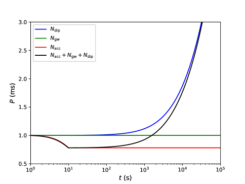
Figure 1: Period of a magnetar as function of time for given Skyrme Lyon (SLy) EOS, $B_{0}=10^{15}\mathrm{G}$, and $\Lambda=0.2$. The solid red, blue, and green lines are the accretion torque, GW radiation torque, and dipole radiation torque, respectively. The black curve is the total contribution from all three.

Figure 1 shows the evolution of the period for given EOS of the NS, strength of the magnetic field, and fraction of poloidal magnetic energy. We find that the accretion torque $N_{\mathrm{acc}}$ is dominant during the spin-up of the magnetar at an early time ($t\lesssim 10$ s) before the available accreted mass is exhausted. At a later time, the angular momentum of the magnetar is carried away mainly via magnetic dipole radiation. The contribution of the GW radiation is small and can be ignored.

As mentioned in Ref. [53], the total perturbation potential is dependent on the angular frequency of the magnetar. Based on Eq.(41), one can easily obtain the evolution of the total perturbation potential with time, or the evolution of $\epsilon_{\mathrm{sta}}$. Combining with Eqs. (8), (16), (29), (35), and (41), one can obtain the evolution of total GW luminosity, which is written as

$$L_{\mathrm{gw}}(t)=-\frac{32}{5}\frac{GI_{0}^{2}}{c^{5}}\left[\epsilon_{\mathrm{acc}}(t)+\epsilon_{\mathrm{mag}}+\epsilon_{\mathrm{sta}}(t)\right]^{2}\Omega(t)^{6}.$$ (42)

Figure 2 shows the evolution of GW luminosity with different magnetic field strengths (e.g., $B_{0}=10^{14}\mathrm{G},5\times 10^{14}\mathrm{G},10^{15}\mathrm{G}$) with fixed $\Lambda=0.2$ and a given EOS. We find that the GW radiation caused by an accretion mountain is stronger than the GW radiation from starquake-induced deformation or magnetically induced deformation for $B_{0}=10^{14}\mathrm{G}$. Because of the hypothesis above that the crust breaking occurred at the equator and the definition of starquake-induced ellipticity in Eq. (22), the $\epsilon_{\rm sta}$ will be negative or positive for $\Omega-\Omega_{0}>0$ and $\Omega-\Omega_{0}<0$, respectively. According to Eq. (16), $\epsilon_{\rm mag}$ is dependent on the value of $\Lambda$, and $\epsilon_{\rm mag}$ is negative and in the same direction as $\epsilon_{\rm acc}$ if $\Lambda<0.385$, and vice versa. Thus, the positive ellipticity of magnetars caused by starquakes and the negative ellipticity of magnetars caused by a larger toroidal magnetic field will cancel each other out when $\Omega<\Omega_{0}$, and the total GW radiation will decrease afterward or even disappear when $\epsilon_{\rm sta}=-\epsilon_{\rm mag}$.

As the strength of the magnetic field increases $(B_{0}=5\times 10^{14}\mathrm{G})$, the GW radiation caused by magnetically induced deformation becomes increasingly strong. $L_{\mathrm{sta}}$ will increase gradually during accretion phase because of increased $\epsilon_{\rm sta}$ when the star spins up. As well, $\epsilon_{\rm sta}$ will gradually decrease or even disappear completely when the accretion stops. When the star spins down, $\epsilon_{\rm sta}$ becomes negative and goes on decreasing, hence $L_{\mathrm{sta}}$ ($\propto\epsilon^{2}_{\rm sta}$) can be increased again. When the strength of the magnetic field is strong enough, i.e. reaching $10^{15}\mathrm{G}$, the GW radiation caused by the magnetically induced deformation is dominant.

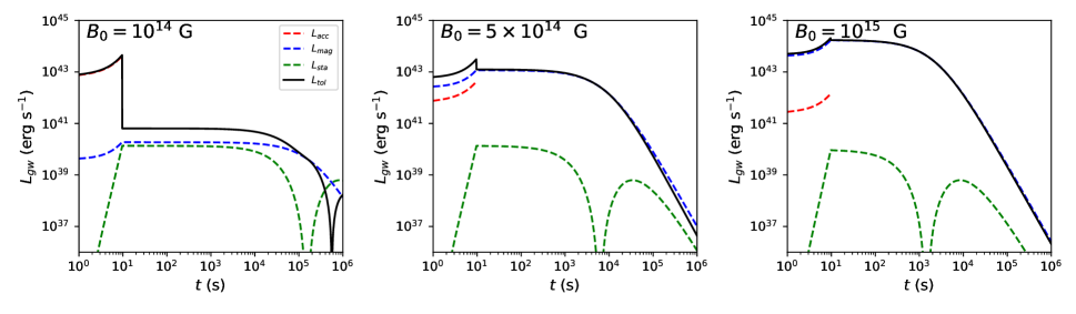
Figure 2: Evolution of GW radiation with fixed $\Lambda=0.2$ and given SLy EOS for different magnetic field strengths ($B_{0}=10^{14}\mathrm{G},5\times 10^{14}\mathrm{G},10^{15}\mathrm{G}$).

In order to test the dependence of the GW radiation on $\Lambda$ with a fixed-strength magnetic field ($B_{0}=5\times 10^{14}\mathrm{G}$) and given EOS, we present the evolution of GW radiation with different $\Lambda$ in Fig. 3. From the MHD simulation point of view, for given different initial magnetic field configurations, $\Lambda$ is as large as 0.8 in a relativistic situation, but in a Newtonian simulation, the $\Lambda$ would stabilize at an equilibrium value of 0.2 [45, 46]. So, we choose $\Lambda=0.2,0.35,0.8$ in our calculations. With a large toroidal component of the magnetic field $\Lambda=0.2$, the contributions to the GW radiation mainly come from $L_{\rm{mag}}$. Decreasing the fraction of the toroidal component (increasing the value of $\Lambda=0.385$) will make the contribution of $L_{\rm mag}$ gradually decrease, and $L_{\rm sta}$ will dominate at later time. For $\Lambda>0.385$, the total GW radiation is dominated by magnetically induced deformation with $\epsilon_{\rm mag}>0$. Therefore, the $L_{\rm tol}$ has an initially sharp drop with $\Lambda=0.8$ due to the offset of $\epsilon_{\rm mag}$ and $-\epsilon_{\rm acc}$.

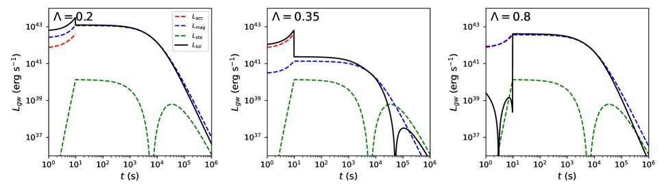
Figure 3: Evolution of GW radiation with fixed $B_{0}=5\times 10^{14}\mathrm{G}$ and given SLy EOS for different poloidal magnetic field components ($\Lambda=0.2$, 0.35, 0.8).

Similarly with Fig. 2 and Fig. 3, we also present the evolution of the GW radiation with different adiabatic indices ($\gamma=2,2.1,\infty$) for SLy EOS and fixed $B_{0}=10^{15}$, $\Lambda=0.2$ in Fig. 4. The response timescale of the density perturbation is approximately equal to the timescale for the system reaching complete thermodynamic equilibrium when the system is perturbed, and it is dependent on the adiabatic index $\gamma$. A larger $\gamma$ corresponds to a shorter response timescale of the density perturbation. Figure 4 shows the results for different adiabatic indices ($\gamma=2,2.1,\infty$). We find that GW radiation from magnetically induced deformation is dominant with $\gamma=2$, but when we increase $\gamma$ from 2 to 2.1, the GW radiation of the starquake-induced deformation strengthens significantly and becomes comparable with $L_{\mathrm{mag}}$. A similar result is also found if we increase $\gamma$ to infinity (see also Ref. [14]). For $\gamma=2.1$ or even infinity, the total GW luminosity rapidly decreases when the magnetar is spun down. At some point, however, $\epsilon_{\mathrm{sta}}$ supported by the centrifugal force perturbation will gradually become stronger, and will decrease until it is comparable with $-\epsilon_{\mathrm{mag}}$. After that, the total GW radiation is dominated by the starquake-induced deformation.

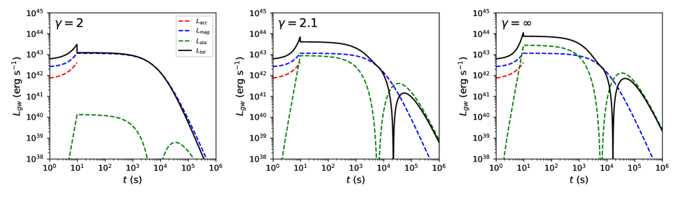
Figure 4: Evolution of GW radiation calculated with different adiabatic indices ($\gamma=2,2.1,\infty$) for SLy EOS and fixed $B_{0}=10^{15}$, $\Lambda=0.2$.

As discussed above, we only adopt one magnetar EOS to do the calculations. Now, to discuss the dependence of the GW radiation on the EOS, we consider 12 EOSs that are reported in the literature [62, 63, 64, 65, 66]. The relevant initial parameters we selected for different EOS are listed in Table 1. The total mass of the neutron star will increase with the accretion, and the neutron star will collapse when the total mass of the neutron star is larger than $M_{\mathrm{TOV}}$. However, the initial mass of the neutron star remains uncertain. In order to test the long-lasting evolution of GW and avoid the neutron star collapse, we choose the initial mass of neutron star as $M_{0}=M_{\mathrm{TOV}}-0.2M_{\odot}$ in our actual calculations. In fact, the masses observed by LIGO and Virgo in NS inspirals are quite high. The merger product is likely to be a supermassive or hypermassive NS which is supported by differential rotation. Further accretion coupled with spin-down would then lead it to collapse to a black hole. Therefore, our estimated of signal duration is optimistic and the signal in actual physical observations may be even shorter. Figure 5 shows the evolution of GW radiation with different EOSs for given $B_{0}=5\times 10^{14}$, $\Lambda=0.2$, and $\gamma=2.1$. We find that the GW radiation from magnetically induced deformation, starquake deformation, and an accretion mountain are not very sensitive to the EOSs we selected.

Table 1: Maximum mass of magnetar for different EOS and corresponding radius.

EOS	$M_{\mathrm{TOV}}$	$R$	$I_{0}$
	$\left(M_{\odot}\right)$	$(\mathrm{km})$	$\left(10^{45}\mathrm{~{}g}\mathrm{~{}cm}^{2}\right)$
BCPM	1.98	9.94	2.86
SLy	2.05	9.99	1.91
BSk20	2.17	10.17	3.50
Shen	2.18	12.40	4.68
APR	2.20	10.00	2.13
BSk21	2.28	11.08	4.37
GM1	2.37	12.05	3.33
DD2	2.42	11.89	5.43
DDME2	2.48	12.09	5.85
AB-N	2.67	12.90	4.30
AB-L	2.71	13.70	4.70
NL3$\omega\rho$	2.75	12.99	7.89

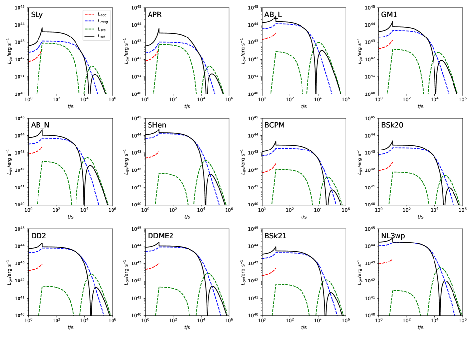
Figure 5: Evolution of GW luminosity with different EOSs for given $B_{0}=5\times 10^{14}\mathrm{G}$, $\Lambda=0.2$, and $\gamma=2.1$.

IV Detection Probability of a GW

One interesting question is that how strong of GW signal is from neutron star. In this section, we will present more details for calculation of the GW radiation.

The characteristic strain of GW from a rotating NS can be estimated as[67, 68, 69, 10]

$$h_{\mathrm{c}}=fh_{0}\sqrt{\frac{dt}{df}}$$ (43)

and

$$h_{0}=\frac{4GI_{0}\epsilon}{Dc^{4}}\Omega^{2}.$$ (44)

$h_{0}$ is GW amplitude emitted by such an object at distance $D$, and $f=\Omega/\pi$ is the rotation frequency. Hence, combining with Eqs. (44) and (41), the characteristic GW strain $h_{\mathrm{c}}$ can be rewritten as

$$h_{\mathrm{c}}=\frac{32\pi^{2}GI_{0}\epsilon}{Dc^{4}}\sqrt{\frac{\pi I_{0}}{N_{\mathrm{tol}}}}f^{3}$$ (45)

The GW strain is dependent on the distance, so we assume that the distance of magnetar is at 10 and 40 Mpc. By adopting the frequency range of GW from $f$=120 to 1000 Hz, one can estimate the maximum value of the strain $h_{\mathrm{c}}$ for different EOSs of NS at distance 10 and 40 Mpc. In Fig. 6, we plot the GW strain sensitivity for aLIGO and the ET. It is clear that the GW strain of magnetar with different EOSs is below the aLIGO noise curve at the distance of 40 Mpc, but it is expected to be detected by aLIGO at 10 Mpc. Moreover, we find that it is expected to be detected by the proposed ET in the future even for the distance of 40 Mpc.

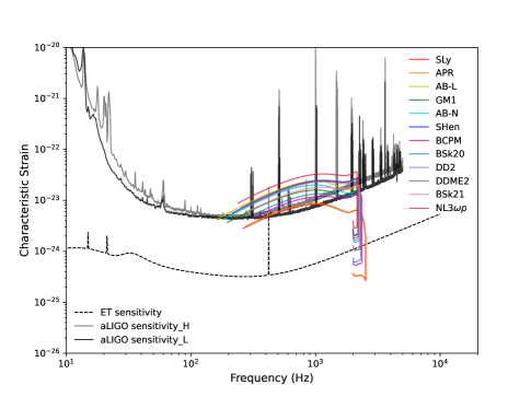
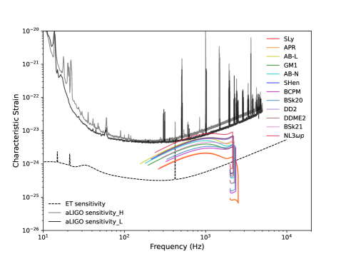
Figure 6: Gravitational-wave strain evolution with frequency of magnetar for different EOSs at distance 10 Mpc (top) and 40 Mpc (bottom). The black dotted line is the sensitivity limits for ET, and the black and gray solid lines are the sensitivity limits for aLIGO-Hanford and aLIGO-Livingston, respectively. The data of the noise curve are taken from Ref. [66].

V Conclusion

A magnetar may survive for hundreds of seconds or longer after a binary neutron star merger or massive star core collapse. Weak GW radiation may be produced by the newborn magnetar due to its deformed structure. In this paper, we have investigated the evolution of the GW radiation of a magnetar by considering different deformations (e.g., magnetically induced deformation, starquake-induced ellipticity, and accretion column-induced deformation). The following interesting results are obtained.

1. For a given magnetar EOS, $B_{0}$, and $\Lambda$, the accretion torque and magnetic dipole radiation are dominant during the spin-up at early times and spin-down at later times, respectively, and the contribution of the GW radiation is small and can be ignored.

2. For a given magnetar EOS and fixed $\Lambda=0.2$, the GW radiation signatures caused by an accretion mountain are stronger than that of starquakes and magnetically induced deformation for $B_{0}=10^{14}\mathrm{G}$. However, with the increased magnetic field strength, the GW radiation caused by magnetically induced deformation gradually becomes dominant.

3. If the SLy EOS, $B_{0}=10^{15}$, and $\Lambda=0.2$ are fixed, the GW radiation from a magnetically induced deformation is dominant for $\gamma=2$. However, when we change $\gamma$ slightly from 2 to 2.1, the GW radiation of the starquake-induced deformation strengthens significantly and comparably with $L_{\rm mag}$ and $L_{\rm acc}$. A similar result also exists even when $\gamma$ increases to infinity.

4. We selected 12 EOSs for given $B_{0}=5\times 10^{14}$, $\Lambda=0.2$, and $\gamma=2.1$. We find that the GW radiation from magnetically induced deformation, starquake deformation, and an accretion mountain are not very sensitive to the different EOSs we selected.

5. Finally, we calculate the GW strain with different EOSs, and find that it is difficult to be detected by aLIGO at 40 Mpc unless we move it closer to 10 Mpc. However, it is expected to be detected by ET in the future.

In our calculations, we do not consider the evolution of the magnetic field when we calculate the GW radiation of magnetically induced deformation. There are two main reasons: One is that we do not know the details of the magnetic field evolution. The other is that the timescale of the magnetic field decay is long ($~{}10^{4}\mathrm{yr}$) [70], and in fact is much longer than the lifetime of a newborn magnetar that we consider. Hence, we do not consider the evolution $\epsilon_{\mathrm{mag}}$ with the magnetic field.

Although the GW radiation from a newborn magnetar has still not been detected by the current aLIGO and Virgo detectors, it plays a very important role in understanding the physics of neutron stars. The GW radiation is expected to be detected by the next generation of more sensitive GW detectors (e.g., ET), and a multimessenger detection will allow us to understand more details of the physics of neutron stars.