Depletion of Resources by a Population of Diffusing Species

Abstract

Depletion of natural and artificial resources is a fundamental problem and a potential cause of economic crises, ecological catastrophes, and death of living organisms. Understanding the depletion process is crucial for its further control and optimized replenishment of resources. In this paper, we investigate a stock depletion by a population of species that undergo an ordinary diffusion and consume resources upon each encounter with the stock. We derive the exact form of the probability density of the random depletion time, at which the stock is exhausted. The dependence of this distribution on the number of species, the initial amount of resources, and the geometric setting is analyzed. Future perspectives and related open problems are discussed.

I Introduction

How long does it take to deplete a finite amount of resources? This fundamental question naturally appears in many aspects of our everyday life and in various disciplines, including economics and ecology. On a global scale, it may concern renewable and non-renewable natural resources such as water, oil, forests, minerals, food, as well as extinction of wildlife populations or fish stocks Mangel85 ; Wada10 ; Dirzo14 . On a local scale, one may think of depletion-controlled starvation of a forager due to the consumption of environmental resources Benichou14 ; Chupeau16 ; Benichou16 ; Chupeau17 ; Bhat17 ; Benichou18 that poses various problems of optimal search and exploration Viswanathan ; Viswanathan99 ; Benichou11 ; Gueudre14 . On even finer, microscopic scale, the depletion of oxygen, glucose, ions, ATP molecules and other chemical resources is critical for life and death of individual cells Fitts94 ; Parekh97 ; Ha99 ; Clapham07 . A reliable characterization of the depletion time, i.e., the instance of an economical crisis, an ecological catastrophe, or the death of a forager or a cell due to resources extinction, is a challenging problem, whose solution clearly depends on the considered depletion process.

In this paper, we investigate a large class of stock depletion processes inspired from biology and modeled as follows: there is a population of $N$ independent species (or particles) searching for a spatially localized stock of resources located on the impenetrable surface of a bulk region (Fig. 1). Any species that has reached the location of the stock, receives a unit of resource and continues its motion. The species are allowed to return any number of times to the stock, each time getting a unit of resource, independently of its former delivery history and of other species. This is a simple yet rich model of a diffusion-controlled release of non-renewable resources upon request. While the applicability of this simplistic model for a quantitative description of natural depletion phenomena is debatable, its theoretical analysis can reveal some common, yet unexplored features of the general stock depletion problem.

If the stock can be modeled as a node on a graph, which is accessed by $N$ random walkers, the stock depletion problem is equivalent to determining the first time when the total number of visits of that site (or a group of sites) exceeds a prescribed threshold Spitzer ; Condamin05 ; Condamin07 . In turn, for continuous-space dynamics, two situations have to be distinguished: (i) The stock is a bulk region, through which the species can freely diffuse; in this case, each species is continuously receiving a fraction of resources as long as it stays within the stock region; the total residence time (also known as occupation or sojourn time) spent by $N$ species inside the stock region can be considered as a proxy for the number of released resources, an one is interested in the first time when this total residence time exceeds a prescribed threshold. The distribution of the residence time for single and multiple particles has been thoroughly investigated Darling57 ; Ray63 ; Knight63 ; Agmon84 ; Berezhkovskii98 ; Dhar99 ; Yuste01 ; Godreche01 ; Majumdar02 ; Benichou03 ; Grebenkov07a ; Burov07 ; Burov11 . (ii) Alternatively, the stock can be located on the impenetrable surface of a bulk region, in which case the species gets a unit of resources at each encounter with that boundary region (Fig. 1); the total number of encounters with the stock region, which is a natural proxy for the number of released resources, is characterized by the total boundary local time $\ell_{t}$ spent by all species on the stock region Levy ; Ito ; Grebenkov07a ; Grebenkov19b ; Grebenkov21a . In this paper, we focus on this yet unexplored setting and aim at answering the following question: If the amount of resources is limited, when does the stock become empty? The time of the stock depletion can be formally introduced as the first-crossing time of a given threshold $\ell$ (the initial amount of resources on the stock) by $\ell_{t}$:

$${\mathcal{T}}_{\ell,N}=\inf\{t>0~{}:~{}\ell_{t}>\ell\}.$$ (1)

We investigate the probability density of this random variable and its dependence on the number $N$ of diffusing species, the initial amount of resources $\ell$, and the geometric setting in which search occurs. We also show how this problem generalizes the extreme first-passage time statistics that got recently considerable attention Weiss83 ; Basnayake19 ; Lawley20 ; Lawley20b ; Lawley20c ; Bray13 ; Majumdar20 ; Grebenkov20d .

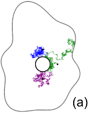
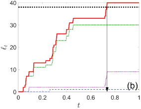
Figure 1: Schematic illustration of a stock depletion problem. (a) Random trajectories of three species diffusing in a bounded domain with the reflecting boundary (shown in gray); at each encounter with the stock region (black circle), one unit of resources is consumed; here, the species are released at different starting points (indicated by small black disks) for a better visualization. (b) The number of consumed resources (thick solid red curve), $\ell_{t}$, as a function of time, and a prescribed threshold (thick dotted black horizontal line), $\ell$, of initially available resources on the stock region; the arrow indicates the first-crossing time ${\mathcal{T}}_{\ell,N}$ when the stock is depleted. Thin curves show the resources $\ell_{t}^{i}$ consumed by individual species.

II Model and general solution

We assume that $N$ independent point-like particles are released at time $t=0$ from a fixed starting point $\bm{x}_{0}\in\Omega$ inside an Euclidean domain $\Omega\subset{\mathbb{R}}^{d}$ with a smooth boundary $\partial\Omega$ (Fig. 1). Each of these particles undertakes an ordinary diffusion inside $\Omega$ with diffusion coefficient $D$ and normal reflections on the impenetrable boundary $\partial\Omega$. Let $\Gamma\subset\partial\Omega$ denote a stock region (that we will also call a target), on which resources are distributed. For each particle $i$, we introduce its boundary local time $\ell_{t}^{i}$ on the stock region $\Gamma$ as $\ell_{t}^{i}=\lim\limits_{a\to 0}a\,\mathcal{N}_{t}^{a,i}$, where $\mathcal{N}_{t}^{a,i}$ is the number of downcrossings of a thin boundary layer of width $a$ near the stock region, $\Gamma_{a}=\{\bm{x}\in\Omega~{}:~{}|\bm{x}-\Gamma|<a\}$, up to time $t$ Levy ; Ito ; Grebenkov07a ; Grebenkov19b ; Grebenkov21a . In other words, $\mathcal{N}_{t}^{a,i}$ represents the number of encounters of the $i$-th particle with the stock region $\Gamma$ (see Grebenkov20 for further discussion). While $\mathcal{N}_{t}^{a,i}$ diverges in the limit $a\to 0$ due to the self-similar nature of Brownian motion, rescaling by $a$ yields a well-defined limit $\ell_{t}^{i}$. For a small width $a$, $\mathcal{N}_{t}^{a,i}\approx\ell_{t}^{i}/a$ can thus be interpreted as the number of resources consumed by the $i$-th particle up to time $t$. In the following, we deal directly with the boundary local times $\ell_{t}^{i}$, which can be easily translated into $\mathcal{N}_{t}^{a,i}$ for any small $a$.

For a single particle, the probability distribution of the random process $\ell_{t}^{i}$ was studied in Grebenkov07a ; Grebenkov19b ; Grebenkov21a . In particular, the moment-generating function of $\ell_{t}^{i}$ was shown to be

$${\mathbb{E}}_{\bm{x}_{0}}\{e^{-q\ell_{t}^{i}}\}=S_{q}(t|\bm{x}_{0}),$$ (2)

where $S_{q}(t|\bm{x}_{0})$ is the survival probability, which satisfies the (backward) diffusion equation

$$\partial_{t}S_{q}(t|\bm{x}_{0})=D\Delta S_{q}(t|\bm{x}_{0})\qquad(\bm{x}_{0}\in\Omega),$$ (3)

with the initial condition $S_{q}(0|\bm{x}_{0})=1$ and the mixed Robin-Neumann boundary condition:

$$\left.(\partial_{n}+q)S_{q}(t|\bm{x}_{0})\right|_{\Gamma} =0,$$ (4a)

$$\left.\partial_{n}S_{q}(t|\bm{x}_{0})\right|_{\partial\Omega\backslash\Gamma} =0$$ (4b)

(for unbounded domains, the regularity condition $S_{q}(t|\bm{x}_{0})\to 1$ as $|\bm{x}_{0}|\to\infty$ is also imposed). Here $\Delta$ is the Laplace operator, and $\partial_{n}$ is the normal derivative at the boundary oriented outward the domain $\Omega$. The survival probability of a diffusing particle in the presence of a partially reactive target has been thoroughly investigated Collins49 ; Sano79 ; Sano81 ; Shoup82 ; Zwanzig90 ; Sapoval94 ; Filoche99 ; Sapoval02 ; Grebenkov03 ; Berezhkovskii04 ; Grebenkov05 ; Grebenkov06a ; Traytak07 ; Bressloff08 ; Lawley15 ; Galanti16 ; Lindsay17 ; Bernoff18b ; Grebenkov17 ; Grebenkov19d ; Guerin21 . In particular, the parameter $q\geq 0$ characterizes the reactivity of the target, ranging from an inert target for $q=0$ to a perfect sink or trap for $q=\infty$. While we speak here about a reactive target in the context of the survival probability, there is no reaction in the stock depletion problem, in which the stock region is inert. In other words, we only explore the fundamental relation (2) between the survival probability and the moment-generating function ${\mathbb{E}}_{\bm{x}_{0}}\{e^{-q\ell_{t}^{i}}\}$ in order to determine the probability density of the boundary local time $\ell_{t}^{i}$ for a single particle, as well as the probability density of the associated first-crossing time Grebenkov20 ; Grebenkov20b .

The amount of resources consumed up to time $t$ is modeled by the total boundary local time,

$$\ell_{t}=\ell_{t}^{1}+\ldots+\ell_{t}^{N},$$ (5)

spent by all species on the stock region. As the individual boundary local times $\ell_{t}^{i}$ are independent, the moment-generating function of $\ell_{t}$ reads

$${\mathbb{E}}_{\bm{x}_{0}}\{e^{-q\ell_{t}}\}=\bigl{(}{\mathbb{E}}_{\bm{x}_{0}}\{e^{-q\ell_{t}^{1}}\}\bigr{)}^{N}=\bigl{[}S_{q}(t|\bm{x}_{0})\bigr{]}^{N},$$ (6)

from which the probability density $\rho_{N}(\ell,t|\bm{x}_{0})$ of $\ell_{t}$ is formally obtained via the inverse Laplace transform with respect to $q$:

$$\rho_{N}(\ell,t|\bm{x}_{0})={\mathcal{L}}_{q,\ell}^{-1}\bigl{\{}[S_{q}(t|\bm{x}_{0})]^{N}\bigr{\}}.$$ (7)

Since the total boundary local time is a non-decreasing process, the cumulative distribution function of the first-crossing time ${\mathcal{T}}_{\ell,N}$, defined by Eq. (1), is

$$Q_{N}(\ell,t|\bm{x}_{0})={\mathbb{P}}_{\bm{x}_{0}}\{{\mathcal{T}}_{\ell,N}<t\}={\mathbb{P}}_{\bm{x}_{0}}\{\ell_{t}>\ell\},$$ (8)

from which Eq. (7) implies

$$Q_{N}(\ell,t|\bm{x}_{0})=1-{\mathcal{L}}_{q,\ell}^{-1}\biggl{\{}\frac{[S_{q}(t|\bm{x}_{0})]^{N}}{q}\biggr{\}}.$$ (9)

In turn, the probability density of the first-crossing time is obtained by time derivative:

$$U_{N}(\ell,t|\bm{x}_{0})=\partial_{t}Q_{N}(\ell,t|\bm{x}_{0})={\mathcal{L}}_{q,\ell}^{-1}\biggl{\{}-\partial_{t}\frac{[S_{q}(t|\bm{x}_{0})]^{N}}{q}\biggr{\}}.$$ (10)

Equations (9, 10) that fully characterize the depletion time ${\mathcal{T}}_{\ell,N}$ in terms of the survival probability $S_{q}(t|\bm{x}_{0})$ of a single particle, present the first main result.

In the limit $\ell\to 0$, Eq. (10) becomes

$$U_{N}(0,t|\bm{x}_{0})=-\partial_{t}[S_{\infty}(t|\bm{x}_{0})]^{N},$$ (11)

i.e., we retrieved the probability density of the fastest first-passage time among $N$ particles to a perfectly absorbing target: ${\mathcal{T}}_{0,\ell}=\min\{\tau^{1}_{\infty},\ldots,\tau^{N}_{\infty}\}$, where $\tau^{i}_{\infty}=\inf\{t>0~{}:~{}\bm{X}_{t}^{i}\in\Gamma\}$ is the first-passage time of the $i$-th particle to $\Gamma$ Weiss83 ; Basnayake19 ; Lawley20 ; Lawley20b ; Lawley20c . Our analysis thus extends considerably the topic of extreme first-passage time statistics beyond the first arrival. More generally, replacing a fixed threshold $\ell$ by a random threshold $\hat{\ell}$ allows one to implement partially reactive targets and various surface reaction mechanisms Grebenkov20 . For instance, if $\hat{\ell}$ is an exponentially distributed variable with mean $1/q$, i.e., ${\mathbb{P}}\{\hat{\ell}>\ell\}=e^{-q\ell}$, then the probability density of the first-crossing time ${\mathcal{T}}_{\hat{\ell},N}$ of the random threshold $\hat{\ell}$ is obtained by averaging $U_{N}(\ell,t|\bm{x}_{0})$ with the density $qe^{-q\ell}$ of $\hat{\ell}$ that yields according to Eq. (10):

$$\int\limits_{0}^{\infty}d\ell\,qe^{-q\ell}\,U_{N}(\ell,t|\bm{x}_{0})=-\partial_{t}\bigl{[}S_{q}(t|\bm{x}_{0})\bigr{]}^{N}.$$ (12)

One can notice that the right-hand side is precisely the probability density of the minimum of $N$ independent first-passage times, $\tau^{1}_{q},\ldots,\tau^{N}_{q}$, to a partially reactive target with reactivity parameter $q$. In other words, we conclude that

$${\mathcal{T}}_{\hat{\ell},N}=\min\{\tau^{1}_{q},\ldots,\tau^{N}_{q}\}.$$ (13)

In turn, the individual first-passage times can also be defined by using the associated boundary local times as $\tau^{i}_{q}=\inf\{t>0~{}:~{}\ell_{t}^{i}>\hat{\ell}^{i}\}$, where $\hat{\ell}^{1},\ldots,\hat{\ell}^{N}$ are independent exponential random variables with the mean $1/q$ Grebenkov20 . Interestingly, while every $\tau^{i}_{q}$ is defined as the time of the first crossing of a random threshold $\hat{\ell}^{i}$ by $\ell_{t}^{i}$ independently from each other, their minimum can be defined via Eq. (13) as the first crossing of the total boundary local time of a random threshold $\hat{\ell}$ with the same $q$.

While the above extension to multiple particles may look simple, getting the actual properties of the probability density $U_{N}(\ell,t|\bm{x}_{0})$ is challenging. In fact, the survival probability $S_{q}(t|\bm{x}_{0})$ depends on $q$ implicitly, through the Robin boundary condition (4a), except for a few cases (see two examples in Appendices A and B). In the following, we first describe some general properties and then employ Eq. (10) to investigate the short-time and long-time asymptotic behaviors of the probability density $U_{N}(\ell,t|\bm{x}_{0})$ to provide a comprehensive view onto the depletion stock problem.

II.1 General properties

Let us briefly discuss several generic properties of the cumulative distribution function $Q_{N}(\ell,t|\bm{x}_{0})$. Since the total boundary local time is a non-decreasing process, the time of crossing a higher threshold is longer than the time of crossing a lower threshold. In probabilistic terms, this statement reads

$$Q_{N}(\ell_{1},t|\bm{x}_{0})\geq Q_{N}(\ell_{2},t|\bm{x}_{0})\qquad(\ell_{1}<\ell_{2}).$$ (14)

In particular, setting $\ell_{1}=0$ in this inequality yields an upper bound for the cumulative distribution function:

$$1-[S_{\infty}(t|\bm{x}_{0})]^{N}=Q_{N}(0,t|\bm{x}_{0})\geq Q_{N}(\ell,t|\bm{x}_{0}),$$ (15)

where we used the asymptotic behavior of Eq. (9) as $\ell\to 0$. In the same vein, as the total boundary local time $\ell_{t}$ is the sum of non-negative boundary local times $\ell_{t}^{i}$, the cumulative distribution function monotonously increases with $N$:

$$Q_{N_{1}}(\ell,t|\bm{x}_{0})\leq Q_{N_{2}}(\ell,t|\bm{x}_{0})\qquad(N_{1}<N_{2}).$$ (16)

Note also that $Q_{N}(\ell,t|\bm{x}_{0})$ is a monotonously increasing function of time $t$ by definition. In the limit $t\to\infty$, one gets the probability of crossing the threshold $\ell$, i.e., the probability of stock depletion:

$$Q_{N}(\ell,\infty|\bm{x}_{0}) =\int\limits_{0}^{\infty}dt\,U_{N}(\ell,t|\bm{x}_{0})$$

$$=1-{\mathcal{L}}^{-1}_{q,\ell}\biggl{\{}\frac{[S_{q}(\infty|\bm{x}_{0})]^{N}}{q}\biggr{\}}\,.$$ (17)

Here, one can distinguish two situations: (i) if any single particle surely reacts on the partially reactive target $\Gamma$ (i.e., $S_{q}(\infty|\bm{x}_{0})=0$), $\ell_{t}$ will cross any threshold $\ell$ with probability $Q_{N}(\ell,\infty|\bm{x}_{0})=1$; (ii) in contrast, if the single particle can survive forever (i.e., $S_{q}(\infty|\bm{x}_{0})>0$) due to its eventual escape to infinity, then the crossing probability is strictly less than $1$. In the latter case, the density $U_{N}(\ell,t|\bm{x}_{0})$ is not normalized to $1$ given that the first-crossing time can be infinite with a finite probability:

$${\mathbb{P}}_{\bm{x}_{0}}\{{\mathcal{T}}_{\ell,N}=\infty\}=1-Q_{N}(\ell,\infty|\bm{x}_{0}).$$ (18)

The probability density $U_{N}(\ell,t|\bm{x}_{0})$ also allows one to compute the positive integer-order moments of the first-crossing time (whenever they exist):

$${\mathbb{E}}_{\bm{x}_{0}}\bigl{\{}[{\mathcal{T}}_{\ell,N}]^{k}\bigr{\}} =\int\limits_{0}^{\infty}dt\,t^{k}\,U_{N}(\ell,t|\bm{x}_{0})$$ (19a)

$$=k\int\limits_{0}^{\infty}dt\,t^{k-1}\,\bigl{(}1-Q_{N}(\ell,t|\bm{x}_{0})\bigr{)},$$ (19b)

for $k=1,2,\ldots$, where the second relation is obtained by integrating by parts under the assumption that $Q_{N}(\ell,\infty|\bm{x}_{0})=1$ (otherwise the moments would be infinite). Applying the inequality (14), we deduce the monotonous behavior of all (existing) moments with respect to $\ell$:

$${\mathbb{E}}_{\bm{x}_{0}}\bigl{\{}[{\mathcal{T}}_{\ell_{1},N}]^{k}\bigr{\}}\leq{\mathbb{E}}_{\bm{x}_{0}}\bigl{\{}[{\mathcal{T}}_{\ell_{2},N}]^{k}\bigr{\}}\qquad(\ell_{1}<\ell_{2}).$$ (20)

Expectedly, the moments of the fastest first-passage time ${\mathcal{T}}_{0,N}$ appear as the lower bounds:

$${\mathbb{E}}_{\bm{x}_{0}}\bigl{\{}[{\mathcal{T}}_{0,N}]^{k}\bigr{\}}\leq{\mathbb{E}}_{\bm{x}_{0}}\bigl{\{}[{\mathcal{T}}_{\ell,N}]^{k}\bigr{\}}.$$ (21)

We stress, however, that the computation and analysis of these moments is in general rather sophisticated, see an example in Appendix A.4 for diffusion on the half-line.

II.2 Short-time behavior

The short-time behavior of $U_{N}(\ell,t|\bm{x}_{0})$ strongly depends on whether the species are initially released on the stock region or not. Indeed, if $\bm{x}_{0}\notin\Gamma$, the species need first to arrive onto the stock region to initiate its depletion. Since the survival probability is very close to $1$ at short times, one can substitute

$$[S_{q}(t|\bm{x}_{0})]^{N}=\bigl{(}1-(1-S_{q}(t|\bm{x}_{0}))\bigr{)}^{N}\approx 1-N\bigl{(}1-S_{q}(t|\bm{x}_{0})\bigr{)}$$

into Eq. (10) to get the short-time behavior

$$U_{N}(\ell,t|\bm{x}_{0})\approx N\,U_{1}(\ell,t|\bm{x}_{0})\qquad(t\to 0).$$ (22)

As the crossing of any threshold $\ell$ by any species is highly unlikely at short times, the presence of $N$ independent species yields an $N$-fold increase of the probability of such a rare event. In fact, the exact solution (42) for diffusion on the half-line allows one to conjecture the following short-time asymptotic behavior in a general domain:

$$U_{1}(\ell,t|\bm{x}_{0})\propto t^{-\alpha}\,e^{-(\delta+\ell)^{2}/(4Dt)}\qquad(t\to 0),$$ (23)

where $\delta$ is the distance from the starting point $\bm{x}_{0}$ to the stock region $\Gamma$, and $\propto$ means proportionality up to a numerical factor independent of $t$ (as $t\to 0$). The exponent $\alpha$ of the power-law prefactor may depend on the domain, even though we did not observe other values than $\alpha=3/2$ for basic examples. The main qualitative argument in favor of this relation is that, at short times, any smooth boundary looks as locally flat so that the behavior of reflected Brownian motion in its vicinity should be close to that in a half-space, for which the exact solution (42) is applicable (given that the lateral displacements of the particle do not affect the boundary local time). In particular, one may expect that the geometrical structure of the domain and of the stock region may affect only the proportionality coefficient in front of this asymptotic form. For instance, the exact solution (34) for diffusion outside a ball of radius $R$ contains the supplementary factor $e^{-\ell/R}R/|\bm{x}_{0}|$, which is not present in the one-dimensional setting. Similarly, the short-time asymptotic relation for $U_{1}(\ell,t|\bm{x}_{0})$ in the case of diffusion outside a disk of radius $R$, that was derived in Grebenkov21a , has the factor $e^{-\ell/(2R)}(R/|\bm{x}_{0}|)^{1/2}$. In both cases, the additional, non-universal prefactor depends on the starting point $|\bm{x}_{0}|$ and accounts for the curvature of the boundary via $e^{-\ell/R}$ or $e^{-\ell/(2R)}$. Further development of asymptotic tools for the analysis of the short-time behavior of $U_{1}(\ell,t|\bm{x}_{0})$ in general domains presents an interesting perspective.

The situation is different when the species are released on the stock region ($\bm{x}_{0}\in\Gamma$) so that the depletion starts immediately. The analysis of the short-time behavior is more subtle, while the effect of $N$ is much stronger. In Appendix A.3, we derived the short-time asymptotic formula (67) by using the explicit form of the survival probability for diffusion on the half-line with the stock region located at the origin. This behavior is valid in the general case because a smooth boundary of the stock region “looks” locally flat at short times. Moreover, the effect of local curvature can be partly incorporated by rewriting the one-dimensional result as

$$U_{N}(t,\ell|\bm{x}_{0})\simeq 2^{N-1}\,N\,U_{1}(Nt,\ell|\bm{x}_{0})\quad(t\to 0).$$ (24)

i.e., the effect of $N$ independent species is equivalent at short times to an $N$-fold increase of time $t$ for a single species and a multiplication by a factor $2^{N-1}N$ whose probabilistic origin is clarified in Appendix A.3.

As the cumulative distribution function $Q_{N}(\ell,t|\bm{x}_{0})$ is obtained by integrating $U_{N}(\ell,t^{\prime}|\bm{x}_{0})$ over $t^{\prime}$ from $0$ to $t$, one can easily derive its asymptotic behavior from Eqs. (22, 24):

$$Q_{N}(\ell,t|\bm{x}_{0}) \approx NQ_{1}(\ell,t|\bm{x}_{0})\qquad(\bm{x}_{0}\notin\Gamma),$$ (25)

$$Q_{N}(\ell,t|\bm{x}_{0}) \approx 2^{N-1}\,Q_{1}(\ell,Nt|\bm{x}_{0})\quad(\bm{x}_{0}\in\Gamma).$$ (26)

II.3 Long-time behavior

The long-time behavior of the probability density $U_{N}(\ell,t|\bm{x}_{0})$ is related via Eq. (10) to that of the survival probability $S_{q}(t|\bm{x}_{0})$, according to which we distinguish four situations:

$$S_{q}(t|\bm{x}_{0})\simeq\left\{\begin{array}[]{l l}e^{-D\lambda_{0}^{(q)}t}\,\psi_{q}(\bm{x}_{0})&(\textrm{class I}),\\ t^{-\alpha}\,\psi_{q}(\bm{x}_{0})&(\textrm{class II}),\\ (\ln t)^{-\alpha}\psi_{q}(\bm{x}_{0})&(\textrm{class III}),\\ S_{q}(\infty|\bm{x}_{0})+t^{-\alpha}\psi_{q}(\bm{x}_{0})&(\textrm{class IV}),\\ \end{array}\right.$$ (27)

where $\lambda_{0}^{(q)}$ is the smallest eigenvalue of the Laplace operator in $\Omega$ with mixed Robin-Neumann boundary condition (4), $\alpha>0$ is a persistence exponent Redner ; Bray13 ; Levernier19 , and $\psi_{q}(\bm{x}_{0})$ is a domain-specific function of $\bm{x}_{0}$ and $q$. Even though the above list of asymptotic behaviors is not complete (e.g., there is no stretched-exponential behavior observed in disordered configurations of traps Kayser83 ; Kayser84 ), these classes cover the majority of cases studied in the literature. For instance, class I includes all bounded domains, in which the spectrum of the Laplace operator is discrete, allowing for a spectral expansion of the survival probability and yielding its exponentially fast decay as $t\to\infty$. For unbounded domains, the long-time behavior of $S_{q}(t|\bm{x}_{0})$ is less universal and strongly depends on the space dimensionality $d$ and the shape of the domain Redner ; Bray13 ; Levernier19 ; Guerin21 . For instance, class II includes: (a) the half-line or, more generally, a half-space, with $\alpha=1/2$ and explicitly known form of $\psi_{q}(\bm{x}_{0})$ (see Appendix A); (b) a perfectly reactive wedge of angle $\theta$ in the plane, with $\alpha=\pi/(2\theta)$ Redner ; (c) a perfectly reactive cone in three dimensions, with a nontrivial relation between $\alpha$ and the cone angle Redner . The exterior of a disk in the plane and the exterior of a circular cylinder in three dimensions are examples of domains in class III Redner ; Levitz08 ; Grebenkov21a . Class IV includes the exterior of a bounded set in three dimensions, in which a particle can escape to infinity and thus never react on the target, with the strictly positive probability $S_{q}(\infty|\bm{x}_{0})$ (see Appendix B).

It is easy to check that Eq. (10) implies the long-time behavior:

$$U_{N}(\ell,t|\bm{x}_{0})\simeq\left\{\begin{array}[]{l l}N\alpha\,t^{-N\alpha-1}\,\Psi_{N}(\bm{x}_{0},\ell)&(\textrm{class II}),\\ \displaystyle\frac{N\alpha\,t^{-1}}{(\ln t)^{N\alpha+1}}\,\Psi_{N}(\bm{x}_{0},\ell)&(\textrm{class III}),\\ N\alpha\,t^{-\alpha-1}\,\Psi_{N}(\bm{x}_{0},\ell)&(\textrm{class IV}),\\ \end{array}\right.$$ (28)

where $\Psi_{N}(\bm{x}_{0},\ell)={\mathcal{L}}_{q,\ell}^{-1}\{[\psi_{q}(\bm{x}_{0})]^{N}/q\}$ for classes II and III, and $\Psi_{N}(\bm{x}_{0},\ell)={\mathcal{L}}_{q,\ell}^{-1}\{[S_{q}(\infty|\bm{x}_{0})]^{N-1}\psi_{q}(\bm{x}_{0})/q\}$ for class IV. One also gets

$$Q_{N}(\ell,t|\bm{x}_{0}) \simeq Q_{N}(\ell,\infty|\bm{x}_{0})$$ (29)

$$-\left\{\begin{array}[]{l l}t^{-N\alpha}\,\Psi_{N}(\bm{x}_{0},\ell)&(\textrm{class II}),\\ \displaystyle(\ln t)^{-N\alpha}\,\Psi_{N}(\bm{x}_{0},\ell)&(\textrm{class III}),\\ N\,t^{-\alpha}\,\Psi_{N}(\bm{x}_{0},\ell)&(\textrm{class IV}),\\ \end{array}\right.$$ (33)

where $Q_{N}(\ell,\infty|\bm{x}_{0})$ is the crossing probability. In turn, the asymptotic behavior in bounded domains (class I) is more subtle and will be addressed elsewhere (see discussions in Grebenkov19b ; Grebenkov20 ; Grebenkov20b ; Grebenkov20c for a single particle).

According to Eqs. (28, 29), the effect of multiple species strongly depends on the geometric structure of the domain. For class II, each added species enhances the power law decrease of the probability density. In particular, the mean first-crossing time is infinite for $N\leq 1/\alpha$ and finite for $N>1/\alpha$. For instance, when the species diffuse on the half-line, the mean first-crossing time is finite for $N>2$ and scales as $N^{-2}$ at large $N$ (see Appendix A.4). Higher-order moments are getting finite as $N$ increases. This effect is greatly diminished for class III, in which the “gain” from having multiple species is just in powers of the logarithm of $t$. As a consequence, the mean first-crossing time remains infinite for any $N$, despite the recurrent nature of diffusion when each species returns infinitely many times to the stock region. For domains of class IV, the transient character of diffusion implies that each species may encounter the stock region a limited number of times before leaving it forever by escaping to infinity with a finite probability. As a consequence, the probability density decays as $t^{-\alpha-1}$ for any $N$, and the number of species affects only the prefactor in front of this universal form. Note that the stock depletion is certain (with probability $1$) for classes II and III; in turn, this probability is below $1$ for class IV but it approaches $1$ exponentially rapidly as $N$ increases, see Eq. (17).

II.4 Example of a spherical stock region

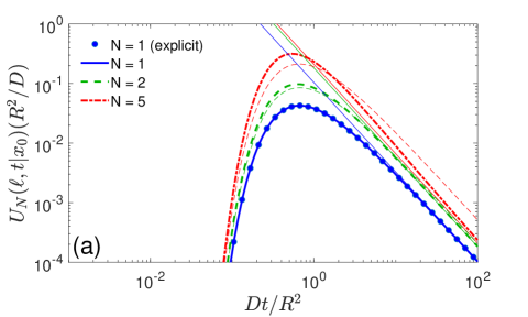
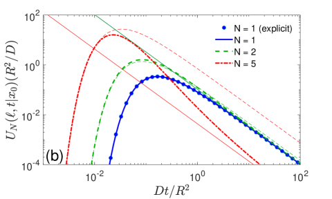
Figure 2: Probability density function $U_{N}(\ell,t|\bm{x}_{0})$ of the first-crossing time ${\mathcal{T}}_{\ell,N}$ for $N$ species diffusing in the exterior of a spherical stock region of radius $R$, with $\ell=R$, and $|\bm{x}_{0}|=2R$ (a) and $|\bm{x}_{0}|=R$ (b). Symbols present the explicit form (34) for a single species, whereas thick lines show the result of numerical integration in Eq. (109), see Appendix C. Thin solid lines indicate the long-time asymptotic relation (28), with $\alpha=1/2$ and $\Psi_{N}(\bm{x}_{0},\ell)$ is given by Eq. (111); in turn, thin dashed lines present the short-time behavior in Eq. (22) for panel (a) and Eq. (24) for panel (b).

To illustrate the properties of the first-crossing time ${\mathcal{T}}_{\ell,N}$, we consider $N$ species diffusing in the three-dimensional space and searching for a spherical stock region of radius $R$. In this setting (class IV), the survival probability $S_{q}(t|\bm{x}_{0})$ has an exact explicit form that allowed us to compute numerically the probability density $U_{N}(\ell,t|\bm{x}_{0})$, see Appendix C for details. For $N=1$, this density gets an explicit form Grebenkov20c :

$$U_{1}(\ell,t|\bm{x}_{0})=\frac{R\,e^{-\ell/R}}{|\bm{x}_{0}|}\,\frac{|\bm{x}_{0}|-R+\ell}{\sqrt{4\pi Dt^{3}}}e^{-(|\bm{x}_{0}|-R+\ell)^{2}/(4Dt)}.$$ (34)

Setting $\ell=0$, one retrieves the probability density of the first-passage time for a perfectly absorbing sphere Smoluchowski17 .

Figure 2 shows the probability density $U_{N}(\ell,t|\bm{x}_{0})$ and its asymptotic behavior for a particular threshold $\ell=R$. When the species start a distance away from the stock region (panel (a)), $U_{N}(\ell,t|r_{0})$ looks as being just “shifted” upwards by increasing $N$, in agreement with the short-time behavior in Eq. (22). In particular, the most probable first-crossing time remains close to that of a single species. Here, the species need first to reach the stock region, so that speed up of the depletion by having many species is modest. The situation is drastically different when the species start on the stock region (panel (b)). In this case, some species may stay close to the stock region, repeatedly returning to it and rapidly consuming its resources. One sees that the total boundary local time reaches a prescribed threshold $\ell$ much faster, and the probability density $U_{N}(\ell,t|r_{0})$ is shifted towards shorter times as $N$ increases. In both panels, the short-time and long-time asymptotic relations derived above are accurate. We stress that the mean first-crossing time and higher-order moments are infinite and thus not informative here. Some other aspects of this depletion problem, such as the cumulative distribution function $Q_{N}(\ell,t|\bm{x}_{0})$, the probability of depletion, and their dependence on $N$, are discussed in Appendix B. In turn, Appendix A presents the study of diffusion on the half-line (class II).

III Discussion and Conclusion

As depletion of resources is one of the major modern problems, numerous former studies addressed various aspects of this phenomenon. For instance, Bénichou et al. investigated depletion-controlled starvation of a diffusing forager and related foraging strategies Benichou14 ; Chupeau16 ; Benichou16 ; Chupeau17 ; Bhat17 ; Benichou18 . These studies focused on the forager itself and on the role of depletion on its survival. In contrast, our emphasis was on the dynamics of stock depletion, i.e., how fast available resources are exhausted by a population of diffusing species. To our knowledge, this problem was not previously addressed, and the present work settles a first theoretical ground for further explorations of this important topic in several directions.

(i) While we focused on a fixed starting point $\bm{x}_{0}$ for all species, an extension of our results to the case of independent randomly distributed starting points is straightforward. In particular, the major difference between Eq. (22) for $\bm{x}_{0}\notin\Gamma$ and Eq. (24) for $\bm{x}_{0}\in\Gamma$ suggests that the form of the initial distribution of $\bm{x}_{0}$ in the vicinity of the stock region may strongly affect the short-time behavior of the probability density $U_{N}(\ell,t|\bm{x}_{0})$.

(ii) For diffusion in bounded domains, the long-time behavior of the probability density $U_{N}(\ell,t|\bm{x}_{0})$ requires a subtle asymptotic analysis of the ground eigenmode of the Laplace operator as a function of the implicit reactivity parameter $q$; the role of the geometric confinement remains to be elucidated.

(iii) In the considered model of non-renewable resources, the stock region is depleted upon each encounter with each diffusing species. This assumption can be relaxed in different ways. For instance, one can consider a continuous-time supply of resources, for which the problem is equivalent to finding the first-crossing time of a deterministic time-dependent threshold $\ell(t)$. Alternatively, replenishment of resources can be realized at random times, as a sort of stochastic resetting. If the resetting times are independent from diffusion of species, one may apply the renewal theory, which was successful in describing diffusion with resetting Evans11 ; Chechkin18 ; Evans20 . Yet another option consists of implementing a dynamic regeneration of consumed resources on the stock region (like a natural regeneration of forests). Finally, one can also include more sophisticated consumption mechanisms when resources are distributed to each species depending on the number of its previous encounters with the stock region (e.g., a species receives less resources at its next return to the stock region). This mechanism and its theoretical implementation resemble the concept of encounter-dependent reactivity in diffusion-controlled reactions Grebenkov20 .

(iv) Another direction consists in elaborating the properties of species. First, one can incorporate a finite lifetime of diffusing species and analyze the stock depletion by “mortal” walkers Meerson15 ; Grebenkov17d . The effect of diversity of species (e.g., a distribution of their diffusion coefficients) can also be analyzed. Second, dynamics beyond ordinary diffusion can be investigated; for instance, the distribution of the boundary local time was recently obtained for diffusion with a gradient drift Grebenkov22 . The knowledge on the survival probability of more sophisticated stochastic dynamics, such as diffusing diffusivity or switching diffusion models Godec17 ; Lanoiselee18 ; Sposini19 ; Grebenkov19f , can potentially be employed in the analysis of the stock depletion problem. Further incorporation of interactions between species (such as communications between ants, bees or birds) may allow to model advanced strategies of faster stock depletion that are common in nature. On the other hand, one can consider multiple stock regions and inquire on their optimal spatial arrangments or replenishment modes to construct sustainable supply networks.

The combination of these complementary aspects of the stock depletion problem will pave a way to understand and control various depletion phenomena in biology, ecology, economics and social sciences.

Appendix A Diffusion on a half-line

In this Appendix, we investigate the stock depletion problem by a population of species diffusing on the half-line, $\Omega={\mathbb{R}}_{+}$. We first recall the basic formulas for a single particle and then proceed with the analysis for $N$ particles. We stress that this setting is equivalent to diffusion in the half-space ${\mathbb{R}}^{d-1}\times{\mathbb{R}}_{+}$ because the boundary local time is not affected by lateral displacements of the particles along the hyperplane ${\mathbb{R}}^{d-1}$.

A.1 Reminder for a single particle

For the positive half-line with partially reactive endpoint $0$, the survival probability reads Redner

$$S_{q}(t|x_{0})=\mathrm{erf}(z_{0})+e^{-z_{0}^{2}}\mathrm{erfcx}\bigl{(}z_{0}+q\sqrt{Dt}\bigr{)},$$ (35)

where $\mathrm{erfcx}(z)=e^{z^{2}}\mathrm{erfc}(z)$ is the scaled complementary error function, and $z_{0}=x_{0}/\sqrt{4Dt}$. One has $S_{q}(t|x_{0})\to 1$ as $q\to 0$, and

$$S_{q}(t|x_{0})\xrightarrow[q\to\infty]{}S_{\infty}(t|x_{0})=\mathrm{erf}(z_{0})+\frac{1}{\sqrt{\pi Dt}}\,q^{-1}+O(q^{-2}),$$ (36)

where we used the asymptotic behavior of $\mathrm{erfcx}(z)$. The probability density of the first-passage time, $H_{q}(t|x_{0})=-\partial_{t}S_{q}(t|x_{0})$, is

$$H_{q}(t|x_{0})=qDe^{-z_{0}^{2}}\biggl{(}\frac{1}{\sqrt{\pi Dt}}-q\,\mathrm{erfcx}\bigl{(}z_{0}+q\sqrt{Dt}\bigr{)}\biggr{)}.$$ (37)

Note also that

$$S_{q}(t|x_{0})\simeq 1-\frac{2\sqrt{Dt}}{x_{0}\sqrt{\pi}}\,\frac{2qDt}{x_{0}+2qDt}\,e^{-x_{0}^{2}/(4Dt)}\quad(t\to 0),$$ (38)

so that the algebraic prefactor in front of $e^{-x_{0}^{2}/(4Dt)}$ is different for perfectly and partially reactive targets. In the long-time limit, one gets

$$S_{q}(t|x_{0})\simeq\frac{x_{0}+1/q}{\sqrt{\pi Dt}}+O(t^{-1})\qquad(t\to\infty),$$ (39)

i.e., the half-line belongs to class II according to our classification in Eq. (27), with

$$\alpha=\frac{1}{2}\,,\qquad\psi_{q}(x_{0})=\frac{x_{0}+1/q}{\sqrt{\pi D}}\,.$$ (40)

The probability density of the boundary local time $\ell_{t}^{1}$ is

$$\rho_{1}(\ell,t|x_{0})=\mathrm{erf}\biggl{(}\frac{x_{0}}{\sqrt{4Dt}}\biggr{)}\delta(\ell)+\frac{\exp\bigl{(}-\frac{(x_{0}+\ell)^{2}}{4Dt}\bigr{)}}{\sqrt{\pi Dt}}\,,$$ (41)

while the probability density of the first-crossing time of a threshold $\ell$ by $\ell_{t}^{1}$ reads Borodin ; Grebenkov20c :

$$U_{1}(\ell,t|x_{0})=(\ell+x_{0})\frac{e^{-(\ell+x_{0})^{2}/(4Dt)}}{\sqrt{4\pi Dt^{3}}}\,.$$ (42)

Note that

$$Q_{1}(\ell,t|x_{0})=\int\limits_{\ell}^{\infty}d\ell^{\prime}\,\rho_{1}(\ell^{\prime},t|x_{0})=\mathrm{erfc}\biggl{(}\frac{x_{0}+\ell}{\sqrt{4Dt}}\biggr{)}.$$ (43)

The most probable first-crossing time corresponding to the maximum of $U_{1}(t,\ell|x_{0})$ is

$$t_{\rm mp,1}=\frac{(x_{0}+\ell)^{2}}{6D}\,.$$ (44)

A.2 PDF of the total boundary local time

The probability density of the total boundary local time $\ell_{t}$ is determined via the inverse Laplace transform in Eq. (7). In Appendix C, we provide an equivalent representation (114) in terms of the Fourier transform, which is more suitable for the following analysis. Substituting $S_{q}(t|x_{0})$ from Eq. (35), we get

$$\rho_{N}(\ell,t|x_{0})=\bigl{(}\mathrm{erf}(z_{0})\bigr{)}^{N}\delta(\ell)+\frac{I_{N}(\ell/\sqrt{Dt},z_{0})}{\sqrt{Dt}}\,,$$ (45)

where

$$I_{N}(\lambda,z_{0})=\int\limits_{-\infty}^{\infty}\frac{dq}{2\pi}\,e^{iq\lambda}$$ (46)

$$\quad\times\biggl{[}\biggl{(}\mathrm{erf}(z_{0})+e^{-z_{0}^{2}}\mathrm{erfcx}(z_{0}+iq)\biggr{)}^{N}-\bigl{(}\mathrm{erf}(z_{0})\bigr{)}^{N}\biggr{]}\,.$$

The small-$\ell$ asymptotic behavior of this density can be obtained as follows. We distinguish two cases: $z_{0}>0$ or $z_{0}=0$. In the former case, we find

$$I_{N}(\lambda,z_{0})=\frac{Ne^{-z_{0}^{2}}\bigl{(}\mathrm{erf}(z_{0})\bigr{)}^{N-1}}{\sqrt{\pi}}+o(1)\qquad(\lambda\to 0),$$ (47)

and thus Eqs. (36, 45) imply in the limit $\ell\to 0$:

$$\rho_{N}(\ell,t|x_{0})\simeq\bigl{(}\mathrm{erf}(z_{0})\bigr{)}^{N}\delta(\ell)+\frac{Ne^{-z_{0}^{2}}\bigl{(}\mathrm{erf}(z_{0})\bigr{)}^{N-1}}{\sqrt{\pi Dt}}+o(1).$$ (48)

In turn, for $z_{0}=0$, one has

$$I_{N}(\lambda,0)=\int\limits_{-\infty}^{\infty}\frac{dq}{2\pi}\,e^{iq\lambda}\biggl{(}\mathrm{erfcx}(iq)\biggr{)}^{N}\,.$$ (49)

Note that $w(q)=\mathrm{erfcx}(-iq)$ is the Faddeeva function, which admits the integral representation:

$$w(q) =\frac{1}{\sqrt{\pi}}\int\limits_{0}^{\infty}dz\,e^{-z^{2}/4+iqz}\,.$$ (50)

For large $|q|$, the imaginary part of $w(q)$ behaves as $1/(q\sqrt{\pi})$, while the real part decays much faster, so that $\mathrm{erfcx}(-iq)\simeq i/(q\sqrt{\pi})$. Using this asymptotic behavior, one can show that

$$I_{N}(\lambda,0)\simeq\frac{\lambda^{N-1}}{\pi^{N/2}\,(N-1)!}\qquad(\lambda\to 0),$$ (51)

from which

$$\rho_{N}(\ell,t|0)\simeq\frac{\bigl{(}\ell/\sqrt{Dt}\bigr{)}^{N-1}}{(N-1)!\,\pi^{N/2}\,\sqrt{Dt}}\qquad(\ell\to 0).$$ (52)

The opposite large-$\ell$ limit relies on the asymptotic analysis of $I_{N}(\lambda,z_{0})$ as $\lambda\to\infty$. We re-delegate the mathematical details of this analysis to Appendix A.5 and present here the final result based on Eq. (85):

$$\rho_{N}(\ell,t|x_{0}) \approx\frac{1}{\sqrt{\pi Dt}}\sum\limits_{n=1}^{N}\binom{N}{n}[\mathrm{erf}(z_{0})]^{N-n}$$

$$\times e^{-(nx_{0}+\ell)^{2}/(4nDt)}\,\frac{2^{n-1}}{\sqrt{n}}\quad(\ell\to\infty)\,.$$ (53)

If $\ell\gg Nx_{0}$, the dominant contribution comes from the term with $n=N$ that simplifies the above expression as:

$$\rho_{N}(\ell,t|x_{0})\approx\frac{2^{N-1}}{\sqrt{\pi NDt}}e^{-(Nx_{0}+\ell)^{2}/(4NDt)}\,.$$ (54)

We emphasize that this result is applicable for any $N$; moreover, for $N=1$, this asymptotic formula is actually exact, see Eq. (41). This is in contrast with a Gaussian approximation which was earlier suggested in the long-time limit for the case of a single particle Grebenkov07a ; Grebenkov19b . In fact, as the particles are independent, the sum of their boundary local times $\ell_{t}^{i}$ can be approximated by a Gaussian variable, i.e.,

$$\rho_{N}(\ell,t|x_{0})\simeq\frac{\exp\bigl{(}-\frac{(\ell-N{\mathbb{E}}_{x_{0}}\{\ell_{t}^{1}\})^{2}}{2N\mathrm{Var}_{x_{0}}\{\ell_{t}^{1}\}}\bigr{)}}{\sqrt{2\pi N\mathrm{Var}_{x_{0}}\{\ell_{t}^{1}\}}}\qquad(\ell\to\infty).$$ (55)

This relation could also be obtained by using the Taylor expansion of the integrand function in Eq. (46) up to the second order in $q^{2}$ for the evaluation of its asymptotic behavior. The mean and variance of $\ell_{t}^{1}$ that appear in Eq. (55), can be found from the explicit relation (41):

$${\mathbb{E}}_{x_{0}}\{\ell_{t}^{1}\} =\frac{2\sqrt{Dt}}{\sqrt{\pi}}\,e^{-z_{0}^{2}}-x_{0}\mathrm{erfc}(z_{0}),$$ (56)

$${\mathbb{E}}_{x_{0}}\{[\ell_{t}^{1}]^{2}\} =(x_{0}^{2}+2Dt)\mathrm{erfc}(z_{0})-\frac{2x_{0}\sqrt{Dt}}{\sqrt{\pi}}\,e^{-z_{0}^{2}},$$ (57)

from which the variance follows as

$$\mathrm{Var}_{x_{0}}\{\ell_{t}^{1}\}={\mathbb{E}}_{x_{0}}\{[\ell_{t}^{1}]^{2}\}-\bigl{(}{\mathbb{E}}_{x_{0}}\{\ell_{t}^{1}\}\bigr{)}^{2}.$$ (58)

In particular, one gets for $x_{0}=0$:

$${\mathbb{E}}_{0}\{\ell_{t}^{1}\}=\frac{2}{\sqrt{\pi}}\sqrt{Dt}\,,\quad\mathrm{Var}_{0}\{\ell_{t}^{1}\}=2Dt(1-2/\pi).$$ (59)

However, this approximation is applicable either in the large $N$ limit due to the central limit theorem, or in the long-time limit, in which each $\ell_{t}^{i}$ is nearly Gaussian. In particular, the Gaussian approximation (55) does not capture the large-$\ell$ behavior shown in Fig. 3.

Figure 3 illustrates the behavior of the probability density $\rho_{N}(\ell,t|x_{0})$ for several values of $N$. First, one sees that both small-$\ell$ and large-$\ell$ asymptotic relations are accurate. When the particles start away from the stock region (panel (a)), the regular part of $\rho_{N}(\ell,t|x_{0})$ approaches a constant level, which decreases with $N$ according to Eq. (48). In turn, the effect of multiple particles onto the small-$\ell$ behavior is much stronger when the particles are released on the stock region (panel (b)).

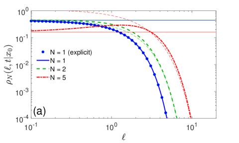
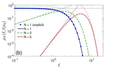
Figure 3: Probability density function $\rho_{N}(\ell,t|x_{0})$ of the total boundary local time $\ell_{t}$ for $N$ particles diffusing on the half-line, with $t=1$, $D=1$, and $x_{0}=1$ (a) and $x_{0}=0$ (b). Symbols present the explicit form (41) for a single particle, whereas thick lines show the numerical integration in Eqs. (45, 46). Thin dashed lines present the large-$\ell$ asymptotic relation (54), while thin solid lines indicate the small-$\ell$ asymptotic relation (48) for $x_{0}=1$ and (52) for $x_{0}=0$, respectively. In panel (a), only the “regular” part is presented, whereas the explicit term with $\delta(\ell)$ is excluded.

A.3 PDF of the first-crossing time

Substituting $S_{q}(t|x_{0})$ from Eq. (35) into the Fourier representation (117) of $U_{N}(\ell,t|x_{0})$, we get

$$U_{N}(\ell,t|x_{0}) =\frac{N\,e^{-z_{0}^{2}}}{t}\int\limits_{-\infty}^{\infty}\frac{dq}{2\pi}\,e^{iq\ell/\sqrt{Dt}}$$

$$\times\biggl{(}\mathrm{erf}(z_{0})+e^{-z_{0}^{2}}\mathrm{erfcx}(z_{0}+iq)\biggr{)}^{N-1}$$

$$\times\biggl{(}\frac{1}{\sqrt{\pi}}-iq\,\mathrm{erfcx}(z_{0}+iq)\biggr{)}.$$

Evaluating the derivative of the function $\mathrm{erfcx}(z)$, one can represent this expression as

$$U_{N}(\ell,t|x_{0}) =\frac{1}{t}\biggl{[}\biggl{(}\frac{\ell}{\sqrt{4Dt}}+Nz_{0}\biggr{)}I_{N}\bigl{(}\ell/\sqrt{Dt},z_{0}\bigr{)}$$

$$-Nz_{0}\mathrm{erf}(z_{0})I_{N-1}\bigl{(}\ell/\sqrt{Dt},z_{0}\bigr{)}\biggr{]},$$ (60)

where $I_{N}(\lambda,z_{0})$ is given by Eq. (46). According to Eq. (45), we can also write

$$U_{N}(\ell,t|x_{0}) =\frac{1}{2t}\biggl{(}(\ell+Nx_{0})\rho_{N}(\ell,t|x_{0})$$

$$-Nx_{0}\,\mathrm{erf}(z_{0})\,\rho_{N-1}(\ell,t|x_{0})\biggr{)}.$$ (61)

In the particular case $x_{0}=0$, one gets a simpler relation

$$U_{N}(\ell,t|0) =\frac{\ell}{2t}\rho_{N}(\ell,t|0).$$ (62)

The long-time asymptotic behavior of $U_{N}(\ell,t|x_{0})$ is determined by the first line in Eq. (28). Substituting $\alpha$ and $\psi_{q}(x_{0})$ from Eq. (40), we find

$$U_{N}(\ell,t|x_{0})\simeq\frac{N\bigl{(}x_{0}/\sqrt{\pi Dt}\bigr{)}^{N}}{2t}\sum\limits_{n=0}^{N}\binom{N}{n}\frac{(\ell/x_{0})^{n}}{n!}\,.$$ (63)

In the limit $x_{0}\to 0$, only the term with $n=N$ survives, yielding as $t\to\infty$

$$U_{N}(\ell,t|0)\simeq\frac{D/\ell^{2}}{2\pi^{N/2}(N-1)!}\,(Dt/\ell^{2})^{-1-N/2}.$$ (64)

As a consequence, the mean first-crossing time is infinite for $N=1$ and $N=2$, but finite for $N>2$ (see Appendix A.4 for details). For $N=1$, one retrieves the typical $t^{-3/2}$ decay of the Lévy-Smirnov probability density of a first-passage time, see Eq. (42).

To get the short-time behavior, we treat separately the cases $x_{0}>0$ and $x_{0}=0$. In the former case, Eqs. (22, 42) imply

$$U_{N}(t,\ell|x_{0})\approx N(\ell+x_{0})\frac{e^{-(\ell+x_{0})^{2}/(4Dt)}}{\sqrt{4\pi Dt^{3}}}\qquad(t\to 0),$$ (65)

The analysis is more subtle for $x_{0}=0$, for which Eq. (60) is reduced to

$$U_{N}(\ell,t|0)=\frac{\ell}{2t\sqrt{Dt}}\,I_{N}\bigl{(}\ell/\sqrt{Dt},0\bigr{)}.$$ (66)

Using the asymptotic relation (87), we get the short-time behavior:

$$U_{N}(\ell,t|0)\simeq 2^{N-1}\,\frac{\ell}{\sqrt{4\pi NDt^{3}}}\,e^{-\ell^{2}/(4NDt)}\quad(t\to 0).$$ (67)

This asymptotic relation coincides with the exact Eq. (42) for $N=1$. More generally, the short-time behavior for $N$ particles is given, up to a multificative factor $2^{N-1}$, by the probability density $U_{1}(\ell,t|0)$ for a single particle but with an $N$-fold increase of the diffusion coefficient.

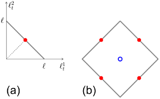
Figure 4: (a) Schematic illustration of crossing of a threshold $\ell$ by $\ell_{t}=\ell_{t}^{1}+\ell_{t}^{2}$ for two particles that corresponds to crossing the gray line. Red filled circle indicates the closest point, through which the crossing is most probable at short times. (b) An equivalent view onto this problem in terms of two-dimensional Brownian motion that starts from the origin (blue circle) and searches to exit the rotated square. Four red filled circles indicate the closest points through which the exit is most probable at short times.

How can one interpret the prefactor $2^{N-1}$? For a single particle, Eq. (42) implies that $U_{1}(\ell,t|0)=\frac{\ell}{\sqrt{4\pi Dt^{3}}}e^{-\ell^{2}/(4Dt)}$ is identical with the probability density of the first-passage time to the origin of the half-line for a particle started a distance $\ell$ away. In other words, the threshold $\ell$ effectively increases the distance from the origin for diffusion on the half-line (see Refs. Sapoval05 ; Grebenkov15 for further discussions on the geometric interpretation of the boundary local time). This follows from the classical fact that the probability law of the boundary local time in this setting is identical to the probability law of the reflected Brownian motion $|W_{t}|$ started from the origin Levy . The reflection symmetry implies that $2U_{1}(\ell,t|0)$ also describes the short-time behavior of the probability density of the first-exit time from the center of the interval $(-\ell,\ell)$. Here, the factor $2$ accounts for the twofold increased probability of the exit event through two equally distant endpoints. This interpretation can be carried on for two particles: the boundary local times $\ell_{t}^{1}$ and $\ell_{t}^{2}$ obey the same probability law as two independent reflected Brownian motions. As a consequence, the first-crossing of a threshold $\ell$ by the total boundary local time $\ell_{t}=\ell_{t}^{1}+\ell_{t}^{2}$ is equivalent to the exit from the square of diameter $2\ell$, rotated by $45^{\circ}$ (Fig. 4). At short times, the exit is most probable through vicinities of 4 points that are the closest to the origin. As a consequence, $U_{2}(\ell,t|0)\approx\tfrac{1}{2}4\frac{\ell_{2}}{\sqrt{4\pi Dt^{3}}}e^{-\ell_{2}^{2}/(4Dt)}$, where $\ell_{2}=\ell/\sqrt{2}$ is the distance from the origin to the edges. For $N$ particles, the closest distance $\ell_{N}=\ell/\sqrt{N}$, whereas there are $2^{N}$ facets of the hypercube, yielding Eq. (67). Even though the exact analogy between the boundary local time and reflected Brownian motion does not carry on beyond the half-line, the short-time asymptotic relation is expected to hold, as illustrated below.

Figure 5 shows the probability density $U_{N}(\ell,t|x_{0})$ for several values of $N$. As expected, the right (long-time) tail of this density becomes steeper as $N$ increases, whereas its maximum is shifted to the left (to smaller times). One sees that both short-time and long-time relations correctly capture the asymptotic behavior of $U_{N}(\ell,t|x_{0})$. At short times, the starting point $x_{0}$ considerably affects the probability density. In fact, when $x_{0}>0$, the short-time behavior is controlled by the arrival of any particle to the stock region, and the presence of $N$ particles simply “shifts” the density upwards, via multiplication by $N$ in Eq. (65). In turn, if the particles start on the stock region ($x_{0}=0$), the number $N$ significantly affects the left tail of the probability density, implying a much faster depletion of resources by multiple particles.

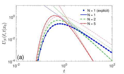
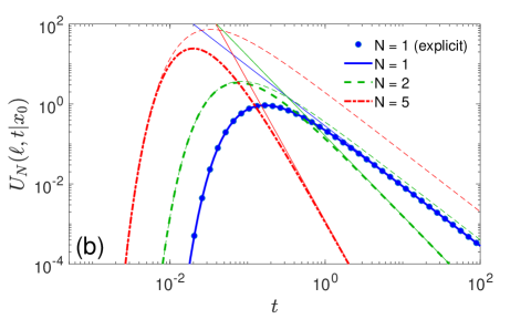
Figure 5: Probability density function $U_{N}(\ell,t|x_{0})$ of the first-crossing time ${\mathcal{T}}_{\ell,N}$ for $N$ particles diffusing on the half-line, with $\ell=1$, $D=1$, and $x_{0}=1$ (a) and $x_{0}=0$ (b). Symbols present the explicit form (42) for a single particle, whereas thick lines show the numerical integration in Eqs. (60, 46). Thin solid lines indicate the long-time asymptotic relation (63) for $x_{0}=1$ and (64) for $x_{0}=0$, respectively. Thin dashed lines present the short-time asymptotic relation (67) for $x_{0}=0$ and (65) for $x_{0}=1$, respectively.

A.4 Mean first-crossing time

Using Eq. (60), one writes the mean first-crossing time as (whenever it exists)

$${\mathbb{E}}_{x_{0}}\{{\mathcal{T}}_{\ell,N}\} =\frac{\ell^{2}}{D}\int\limits_{0}^{\infty}\frac{dy}{y^{3}}\biggl{\{}(y+2N\xi)I_{N}(y,y\xi)$$

$$-2N\xi\,\mathrm{erf}(y\xi)I_{N-1}(y,y\xi)\biggr{\}},$$ (68)

with $\xi=x_{0}/(2\ell)$. Curiously, the expression for the mean first-crossing time is more complicated than that for the probability density. Since the function $I_{N}(\lambda,z_{0})$ is expressed as an integral involving the error function, the analysis of this expression is rather sophisticated. For this reason, we focus on the particular case $x_{0}=0$, for which the above expression is reduced to

$${\mathbb{E}}_{0}\{{\mathcal{T}}_{\ell,N}\}=\frac{\ell^{2}}{D}\int\limits_{0}^{\infty}\frac{dy}{y^{2}}\,\int\limits_{-\infty}^{\infty}\frac{dq}{2\pi}\,e^{-iqy}\biggl{(}\mathrm{erfcx}(-iq)\biggr{)}^{N}\,.$$ (69)

A straightforward exchange of two integrals is not applicable as the integral of $e^{-iqy}/y^{2}$ over $y$ diverges. To overcome this limitation, we regularize this expression by replacing the lower integral limit by $\varepsilon$ and then evaluating the limit $\varepsilon\to 0$:

$${\mathbb{E}}_{0}\{{\mathcal{T}}_{\ell,N}\}=\lim\limits_{\varepsilon\to 0}\frac{\ell^{2}}{D}\int\limits_{-\infty}^{\infty}\frac{dq}{2\pi}\bigl{(}\mathrm{erfcx}(-iq)\bigr{)}^{N}\,F_{\varepsilon}(q),$$ (70)

where

$$F_{\varepsilon}(q)=\frac{e^{-iq\varepsilon}}{\varepsilon}-iq\,{\rm Ei}(1,iq\varepsilon),$$ (71)

with ${\rm Ei}(1,z)$ being the exponential integral. The small-$\varepsilon$ expansion of this function reads

$$F_{\varepsilon}(q)=\varepsilon^{-1}-iq(1-\gamma-\ln(\varepsilon))+iq\ln(iq)+O(\varepsilon).$$ (72)

To get a convergent limit in Eq. (70), one has to show that the integral over $q$ involving the first two terms of this expansion vanishes, i.e., $J_{N}^{(0)}=J_{N}^{(1)}=0$, where

$$J_{N}^{(k)}=\pi^{\frac{N}{2}}\int\limits_{-\infty}^{\infty}\frac{dq}{2\pi}\,q^{k}\bigl{(}\mathrm{erfcx}(-iq)\bigr{)}^{N}.$$ (73)

Let us first consider the integral $J_{N}^{(0)}$. Using the representation (50), we can write

$$J_{N}^{(0)} =\int\limits_{-\infty}^{\infty}\frac{dq}{2\pi}\,\int\limits_{{\mathbb{R}}^{N}_{+}}dz_{1}\ldots dz_{N}\,e^{-\frac{1}{4}(z_{1}^{2}+\ldots+z_{N}^{2})+iq(z_{1}+\ldots+z_{N})}$$

$$=\int\limits_{{\mathbb{R}}^{N}_{+}}dz_{1}\ldots dz_{N}\,e^{-\frac{1}{4}(z_{1}^{2}+\ldots+z_{N}^{2})}\,\delta(z_{1}+\ldots+z_{N}).$$

For $N=1$, this integral yields $J_{1}^{(0)}=\tfrac{1}{2}$, whereas it vanishes for any $N>1$. Similarly, the evaluation of the integral $J_{N}^{(1)}$ involves the derivative of the Dirac distribution and yields $J_{2}^{(1)}=i/2$, while $J_{N}^{(1)}=0$ for any $N>2$. We conclude that the limit in Eq. (70) diverges for $N=1$ and $N=2$, in agreement with the long-time asymptotic behavior (64) of the probability density $U_{N}(\ell,t|x_{0})$. In turn, for $N>2$, the limit is finite and is determined by the integral with the third term in the expansion (72):

$${\mathbb{E}}_{0}\{{\mathcal{T}}_{\ell,N}\}=\frac{\ell^{2}}{D}\int\limits_{-\infty}^{\infty}\frac{dq}{2\pi}\,iq\ln(iq)\,\bigl{(}\mathrm{erfcx}(-iq)\bigr{)}^{N}.$$ (74)

To derive the asymptotic behavior of this integral at large $N$, we use the Taylor expansion for $\ln(w(q))\approx iq\frac{2}{\sqrt{\pi}}-q^{2}(1-2/\pi)+O(q^{3})$ and then approximate the mean as

$${\mathbb{E}}_{0}\{{\mathcal{T}}_{\ell,N}\}\approx\frac{\ell^{2}}{D}\,\frac{\pi}{4N^{2}}\,I_{N},$$ (75)

with

$$I_{N}=\int\limits_{-\infty}^{\infty}\frac{dx}{2\pi}\,ix\ln(ix\sqrt{\pi}/(2N))\,e^{ix}\,e^{-x^{2}/(2z^{2})}\,,$$ (76)

where we rescaled the integration variable as $x=qN(2/\sqrt{\pi})$ and set $z=\sqrt{2N/(\pi-2)}$. As

$$\int\limits_{-\infty}^{\infty}\frac{dx}{2\pi}\,x\,e^{ix}\,e^{-x^{2}/(2z^{2})}\propto e^{-z^{2}/2}$$

is exponentially small for large $N$, one can eliminate the contribution from a numerical constant under the logarithm that allows one to write

$$I_{N}\approx-\int\limits_{0}^{\infty}\frac{dx}{\pi}\,x\,\biggl{(}\frac{\pi}{2}\cos(x)+\sin(x)\,\ln(x)\biggr{)}\,e^{-x^{2}/(2z^{2})}\,.$$ (77)

The first term can be evaluated explicitly and yields $1/2$ as $N\to\infty$. To proceed with the second term, we employ the representation $\ln(x)=\lim\limits_{\varepsilon\to 0}(x^{\varepsilon}-1)/\varepsilon$ and exchange the order of integral and limit:

$$I_{N} \approx\frac{1}{2}-\lim\limits_{\varepsilon\to 0}\frac{1}{\varepsilon}\int\limits_{0}^{\infty}\frac{dx}{\pi}\,x^{1+\varepsilon}\,\sin(x)\,e^{-x^{2}/(2z^{2})}$$

$$=\frac{1}{2}+\lim\limits_{\varepsilon\to 0}\frac{1}{\varepsilon}\,\frac{\sqrt{2}z^{2+\varepsilon}e^{-z^{2}/4}\bigl{(}D_{1+\varepsilon}(-z)-D_{1+\varepsilon}(z)\bigr{)}}{4\sqrt{\pi}\cos(\pi\varepsilon/2)}\,,$$

where $D_{\nu}(z)$ is the Whittaker’s parabolic cylinder function, and we neglected the contribution from $-1/\varepsilon$, which is exponentially small for large $N$. For large $z$, $D_{1+\varepsilon}(z)$ is exponentially small, whereas $D_{1+\varepsilon}(-z)$ behaves as

$$D_{1+\varepsilon}(-z)\approx-\frac{\sqrt{2\pi}}{\Gamma(-1-\varepsilon)}e^{-i\pi(1+\varepsilon)}z^{-2-\varepsilon}e^{z^{2}/4}.$$

As a consequence, one gets

$$I_{N} \approx\frac{1}{2}+\lim\limits_{\varepsilon\to 0}\frac{1}{\varepsilon}\,\frac{e^{-i\pi\varepsilon}}{2\cos(\pi\varepsilon/2)\Gamma(-1-\varepsilon)}=1.$$ (78)

We conclude that

$${\mathbb{E}}_{0}\{{\mathcal{T}}_{\ell,N}\}\approx\frac{\ell^{2}}{D}\,\frac{\pi}{4}\,N^{-2}\qquad(N\gg 1).$$ (79)

While the above derivation is not a mathematical proof, it captures correctly the leading-order behavior of the mean first-crossing time, see Fig. 6(a). A more rigorous derivation and the analysis of the next-order terms present an interesting perspective.

Equation (79) is a rather counter-intuitive result: in fact, one might expect that the “speed up” in crossing the threshold $\ell$ would be proportional to $N$, i.e., the mean time would be inversely proportional to $N$. A similar speed up by $N^{2}$ was observed for the mean first-passage time to a perfectly absorbing target by a population of particles with uniformly distributed initial positions Grebenkov20d ; Madrid20 .

For the case $x_{0}>0$, one can expect even more sophisticated behavior. Indeed, as ${\mathcal{T}}_{0,N}$ is the fastest first-passage time, its mean scales with the logarithm of $N$ Weiss83 ; Basnayake19 ; Lawley20 ; Lawley20b ; Lawley20c

$${\mathbb{E}}_{x_{0}}\{{\mathcal{T}}_{0,N}\}\propto\frac{x_{0}^{2}}{4D\ln N}\qquad(N\gg 1),$$ (80)

i.e., it exhibits a very slow decay with $N$. For any threshold $\ell>0$, the first-crossing time for a single particle naturally splits into two independent parts: the first-passage time from $x_{0}$ to the target, ${\mathcal{T}}_{0,1}$, and then the first-crossing time ${\mathcal{T}}_{\ell,1}^{0}$ for a particle started from the target. The situation is much more complicated for $N$ particles. Intuitively, one might argue that it is enough for a single particle to reach the target and to remain near the target long enough to ensure the crossing of the threshold $\ell$ by the total boundary local time $\ell_{t}$, even if all other particles have not reached the target. In other words, a single particle may do the job for the others (e.g., if $\ell_{t}=\ell_{t}^{1}$ and $\ell_{t}^{i}=0$ for all $i=2,3,\ldots,N$). However, this is not the typical situation that would provide the major contribution to the mean first-crossing time. Indeed, according to the lower bound (21), the mean first-crossing time ${\mathbb{E}}_{x_{0}}\{{\mathcal{T}}_{\ell,N}\}$ cannot decrease with $N$ faster than ${\mathbb{E}}_{x_{0}}\{{\mathcal{T}}_{0,N}\}$, suggesting at least a logarithmically slow decay.

This behavior is confirmed by Fig. 6(a) showing the mean first-crossing time ${\mathbb{E}}_{x_{0}}\{{\mathcal{T}}_{\ell,N}\}$ as a function of $N$ for a fixed value of $\ell$ and several values of the starting point $x_{0}$. When $x_{0}=0$, we observe the earlier discussed power law decay (79). In turn, the decay with $N$ is much slower for $x_{0}>0$. Multiplying ${\mathbb{E}}_{x_{0}}\{{\mathcal{T}}_{\ell,N}\}$ by $\ln N$ and plotting it as a function of $1/\ln N$ (Fig. 6(b)), we confirm numerically the leading-order logarithmic behavior (80) but with significant corrections.

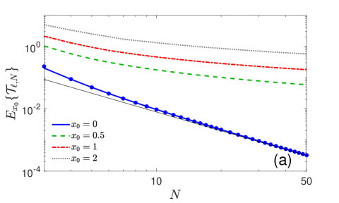
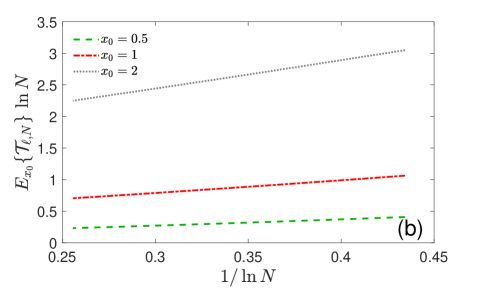
Figure 6: (a) Mean first-crossing time ${\mathbb{E}}_{x_{0}}\{{\mathcal{T}}_{\ell,N}\}$ as a function of the number $N$ of particles diffusing on the half-line, with $\ell=1$, $D=1$, and several values of $x_{0}$ as indicated in the legend. Lines show the result of numerical integration in Eq. (68), with the probability density $U_{N}(\ell,t|x_{0})$ given by Eqs. (60, 46). Symbols present the result of numerical integration in Eq. (75) for the case $x_{0}=0$. Thin black line indicates the asymptotic behavior (79). (b) Another representation of the mean first-crossing time ${\mathbb{E}}_{x_{0}}\{{\mathcal{T}}_{\ell,N}\}$, multiplied by $\ln N$ and shown as a function of $1/\ln N$, for $x_{0}>0$.

A.5 Large-$\lambda$ asymptotic analysis

In this section, we present the details of the large-$\lambda$ asymptotic analysis of the function $I_{N}(\lambda,z_{0})$ defined by Eq. (46). Using the binomial expansion, one gets

$$I_{N}(\lambda,z_{0})=\sum\limits_{n=1}^{N}\binom{N}{n}[\mathrm{erf}(z_{0})]^{N-n}e^{-nz_{0}^{2}}\,i_{n}(\lambda,z_{0}),$$ (81)

where

$$i_{n}(\lambda,z_{0})=\int\limits_{-\infty}^{\infty}\frac{dq}{2\pi}\,e^{iq\lambda}\bigl{[}w(iz_{0}-q)\bigr{]}^{n},$$ (82)

and we used the Faddeeva function $w(z)$ to express $\mathrm{erfcx}(z_{0}+iq)$. To evaluate the large-$\lambda$ asymptotic behavior of the integral $i_{n}(\lambda,z_{0})$, we employ the integral representation (50) of the Faddeeva function:

$$i_{n}(\lambda,z_{0}) =\frac{1}{\pi^{n/2}}\int\limits_{0}^{\infty}dz_{1}\,e^{-z_{1}^{2}/4}\ldots\int\limits_{0}^{\infty}dz_{n}\,e^{-z_{n}^{2}/4}$$

$$\times\delta(z_{1}+\ldots+z_{n}-\lambda)\,e^{-z_{0}(z_{1}+\ldots+z_{n})}$$

$$=e^{-z_{0}\lambda}\,i_{n}(\lambda,0).$$ (83)

We are left therefore with the asymptotic analysis of $i_{n}(\lambda,0)$.

One trivially gets $i_{1}(\lambda,0)=e^{-\lambda^{2}/4}/\sqrt{\pi}$. In general, one has to integrate over the cross-section of the hyperplane $z_{1}+\ldots+z_{n}=\lambda$ with the first (hyper-)octant ${\mathbb{R}}_{+}^{n}$. In the limit $\lambda\to\infty$, the dominant contribution comes from the vicinity of the point $(\lambda,\ldots,\lambda)/n$ of that cross-section that is the closest to the origin. One can therefore introduce new coordinates centered at this point and oriented with this cross-section. For instance, for $n=2$, one uses $z_{1}=\lambda/2+r/\sqrt{2}$ and $z_{2}=\lambda/2-r/\sqrt{2}$ to write

$$i_{2}(\lambda,0) =\frac{1}{\pi}\int\limits_{-\lambda/\sqrt{2}}^{\lambda/\sqrt{2}}\frac{dr}{\sqrt{2}}e^{-\lambda^{2}/8-r^{2}/4}$$

$$=e^{-\lambda^{2}/8}\frac{\sqrt{2}\,\mathrm{erf}(\lambda/\sqrt{8})}{\sqrt{\pi}}\,.$$

As $\lambda\to\infty$, the limits of the above integral can be extended to infinity to get $i_{2}(\lambda,0)\simeq\frac{\sqrt{2}}{\sqrt{\pi}}e^{-\lambda^{2}/8}$.

Similarly, for $n=3$, we use the polar coordinates $(r,\theta)$ in the cross-section

$$z_{1} =\frac{\lambda}{3}+r\biggl{(}\frac{\cos\theta}{\sqrt{2}}+\frac{\sin\theta}{\sqrt{6}}\biggr{)},$$

$$z_{2} =\frac{\lambda}{3}+r\biggl{(}-\frac{2\sin\theta}{\sqrt{6}}\biggr{)},$$

$$z_{3} =\frac{\lambda}{3}+r\biggl{(}-\frac{\cos\theta}{\sqrt{2}}+\frac{\sin\theta}{\sqrt{6}}\biggr{)},$$

such that $z_{1}+z_{2}+z_{3}=\lambda$. As a consequence, we get $z_{1}^{2}+z_{2}^{2}+z_{3}^{2}=\lambda^{2}/3+r^{2}$, from which

$$i_{3}(\lambda,0) \approx\frac{2\pi}{\pi^{3/2}}\int\limits_{0}^{\infty}\frac{dr\,r}{\sqrt{3}}e^{-\lambda^{2}/12-r^{2}/4}$$

$$=e^{-\lambda^{2}/12}\frac{4}{\sqrt{3\pi}}\,.$$

In general, we obtain

$$i_{n}(\lambda,0) \approx\frac{\omega_{n-1}}{\pi^{n/2}}\int\limits_{0}^{\infty}\frac{dr\,r^{n-2}}{\sqrt{n}}e^{-\lambda^{2}/(4n)-r^{2}/4}$$

$$=e^{-\lambda^{2}/(4n)}\frac{2^{n-1}}{\sqrt{\pi n}}\,,$$ (84)

where $\omega_{d}=2\pi^{d/2}/\Gamma(d/2)$ is the area of the unit $d$-dimensional ball. Substituting this asymptotic relation into Eq. (81), we get the large-$\lambda$ behavior:

$$I_{N}(\lambda,z_{0})\approx\sum\limits_{n=1}^{N}\binom{N}{n}[\mathrm{erf}(z_{0})]^{N-n}\,\frac{2^{n-1}}{\sqrt{\pi n}}\,e^{-(nz_{0}+\lambda/2)^{2}/n}\,.$$ (85)

When $\lambda\gg Nz_{0}$, the dominant contribution comes from the term with $n=N$ so that

$$I_{N}(\lambda,z_{0})\approx\frac{2^{N-1}}{\sqrt{\pi N}}\,e^{-(Nz_{0}+\lambda/2)^{2}/N}\,.$$ (86)

In particular, one has

$$I_{N}(\lambda,0)\approx\frac{2^{N-1}}{\sqrt{\pi N}}\,e^{-\lambda^{2}/(4N)}\,.$$ (87)

Appendix B Diffusion outside a ball

In this Appendix, we consider another emblematic example of diffusion in the exterior of a ball of radius $R$: $\Omega=\{\bm{x}\in{\mathbb{R}}^{3}~{}:~{}|\bm{x}|>R\}$.

B.1 Reminder for a single particle

For the case of partially reactive boundary, the survival probability reads Collins49

$$S_{q}(t|r_{0})=1-\frac{R\exp\bigl{(}-\frac{(r_{0}-R)^{2}}{4Dt}\bigr{)}}{r_{0}(1+1/(qR))}\biggl{\{}\mathrm{erfcx}\biggl{(}\frac{r_{0}-R}{\sqrt{4Dt}}\biggr{)}$$

$$-\mathrm{erfcx}\biggl{(}\frac{r_{0}-R}{\sqrt{4Dt}}+\left(1+qR\right)\frac{\sqrt{Dt}}{R}\biggr{)}\biggr{\}}\,,$$ (88)

where $r_{0}=|\bm{x}_{0}|\geq R$ is the radial coordinate of the starting point $\bm{x}_{0}$. As diffusion is transient, the particle can escape to infinity with a finite probability:

$$S_{q}(t|r_{0})\xrightarrow[t\to\infty]{}S_{q}(\infty|r_{0})=1-\frac{R/r_{0}}{1+1/(qR)}>0.$$ (89)

Expanding Eq. (88) in a power series of $1/\sqrt{Dt}$ up to the leading term, one gets the long-time behavior

$$S_{q}(t|r_{0})=S_{q}(\infty|r_{0})+t^{-\alpha}\psi_{q}(r_{0})+O(t^{-1}),$$ (90)

with $\alpha=1/2$ and

$$\psi_{q}(r_{0})=\frac{qR^{2}/r_{0}}{1+qR}\,\frac{r_{0}-R+R/(1+qR)}{\sqrt{\pi D}}\,.$$ (91)

This domain belongs therefore to class IV according to our classification (27).

The probability density of the first-passage time, $H_{q}(t|r_{0})=-\partial_{t}S_{q}(t|r_{0})$, follows immediately (see also Grebenkov18 ):

$$H_{q}(t|r_{0}) =\frac{qD}{r_{0}}e^{-(r_{0}-R)^{2}/(4Dt)}\biggl{\{}\frac{R}{\sqrt{\pi Dt}}$$ (92)

$$-(1+qR)\mathrm{erfcx}\biggl{(}\frac{r_{0}-R}{\sqrt{4Dt}}+(1+qR)\frac{\sqrt{Dt}}{R}\biggr{)}\biggr{\}}.$$

For a perfectly reactive target, one retrieves the Smoluchowski result:

$$S_{\infty}(t|r_{0}) = 1-\frac{R}{r_{0}}\mathrm{erfc}\biggl{(}\frac{r_{0}-R}{\sqrt{4Dt}}\biggr{)},$$ (93)

$$H_{\infty}(t|r_{0}) = \frac{R}{r_{0}}\,\frac{r_{0}-R}{\sqrt{4\pi Dt^{3}}}\,e^{-(r_{0}-R)^{2}/(4Dt)}.$$ (94)

In turn, the probability density $U_{1}(\ell,t|r_{0})$ reads Grebenkov20c

$$U_{1}(\ell,t|r_{0})=\frac{R\,e^{-\ell/R}}{r_{0}}\,\frac{r_{0}-R+\ell}{\sqrt{4\pi Dt^{3}}}e^{-(r_{0}-R+\ell)^{2}/(4Dt)}.$$ (95)

This is a rare example when the probability density $U_{1}(\ell,t|\bm{x}_{0})$ is found in a simple closed form. Setting $\ell=0$, one retrieves the probability density of the first-passage time for a perfectly absorbing sphere Smoluchowski17 . Integrating the probability density over $t$, one gets

$$Q_{1}(\ell,t|r_{0})=\frac{R\,e^{-\ell/R}}{r_{0}}\mathrm{erfc}\biggl{(}\frac{r_{0}-R+\ell}{\sqrt{4Dt}}\biggr{)},$$ (96)

whereas the derivative with respect to $\ell$ yields the continuous part of the probability density $\rho_{1}(\ell,t|\bm{x}_{0})$:

$$\rho_{1}(\ell,t|r_{0})=\biggl{(}1-\frac{R}{r_{0}}\mathrm{erfc}\biggl{(}\frac{r_{0}-R}{\sqrt{4Dt}}\biggr{)}\biggr{)}\delta(\ell)$$ (97)

$$+\frac{e^{-\ell/R}}{r_{0}}\biggl{(}\mathrm{erf}\biggl{(}\frac{r_{0}-R+\ell}{\sqrt{4Dt}}\biggr{)}+\frac{R\,e^{-(r_{0}-R+\ell)^{2}/(4Dt)}}{\sqrt{\pi Dt}}\biggr{)}$$

(here we added explicitly the first term to account for the atom of the probability measure at $\ell=0$). As diffusion is transient, the crossing probability is below $1$:

$$Q_{1}(\ell,\infty|r_{0})=\int\limits_{0}^{\infty}dt\,U_{1}(\ell,t|r_{0})=\frac{R\,e^{-\ell/R}}{r_{0}}<1.$$ (98)

In other words, the density $U_{1}(\ell,t|r_{0})$ is not normalized to $1$ because the diffusing particle can escape to infinity before its boundary local time has reached the threshold $\ell$. Expectedly, the mean first-crossing time is infinite, whereas the most probable first-crossing time, corresponding to the maximum of $U_{1}(\ell,t|r_{0})$, is

$$t_{\rm mp,1}=\frac{(r_{0}-R+\ell)^{2}}{6D}\,.$$ (99)

B.2 The crossing probability

For the case of $N$ particles, we start by analyzing the crossing probability $Q_{N}(\ell,\infty|r_{0})$. Rewriting Eq. (89) as

$$S_{q}(\infty|r_{0})=1-R/r_{0}+\frac{R/r_{0}}{1+qR}\,,$$ (100)

and substituting it into Eq. (17), one gets

$$Q_{N}(\ell,\infty|r_{0})=1-{\mathcal{L}}_{q,\ell}^{-1}\left\{\frac{\bigl{[}1-R/r_{0}+\frac{R/r_{0}}{1+qR}\bigr{]}^{N}}{q}\right\}.$$ (101)

Using the binomial expansion and the identity

$${\mathcal{L}}_{q,\ell}^{-1}\biggl{\{}\frac{1}{q(1+qR)^{n}}\biggr{\}}=1-e^{-\ell/R}\sum\limits_{k=0}^{n-1}\frac{(\ell/R)^{k}}{k!}\,,$$ (102)

we evaluate the inverse Laplace transform of each term that yields after re-arrangment of terms:

$$Q_{N}(\ell,\infty|r_{0}) =e^{-\ell/R}\sum\limits_{k=0}^{N-1}\frac{(\ell/R)^{k}}{k!}$$

$$\times\biggl{(}1-\sum\limits_{n=0}^{k}\binom{N}{n}\alpha^{n}(1-\alpha)^{N-n}\biggr{)},$$ (103)

with $\alpha=R/r_{0}$. For $N=1$, we retrieve Eq. (98). At $r_{0}=R$, one gets a simpler relation

$$Q_{N}(\ell,\infty|R)=e^{-\ell/R}\sum\limits_{k=0}^{N-1}\frac{(\ell/R)^{k}}{k!}\,.$$ (104)

For a fixed $\ell/R$ and large $N$, one has

$$Q_{N}(\ell,\infty|R)\simeq 1-\frac{(\ell/R)^{N}e^{-\ell/R}}{N!}\qquad(N\to\infty),$$ (105)

i.e., the crossing probability rapidly approaches $1$.

Figure 7 illustrates the behavior of the crossing probability $Q_{N}(\ell,\infty|r_{0})$ as a function of $N$. One sees that $Q_{N}(\ell,\infty|r_{0})$ monotonously grows with $N$ and rapidly approaches $1$, whereas the threshold $\ell$ and the starting point $\bm{x}_{0}$ determine how fast this limit is reached.

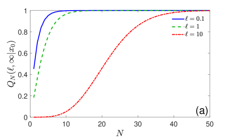
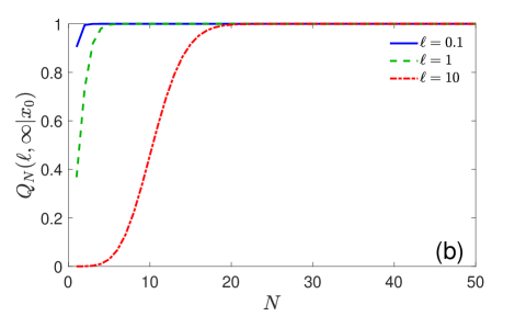
Figure 7: Crossing probability $Q_{N}(\ell,\infty|\bm{x}_{0})$ for $N$ particles diffusing in the exterior of a ball of radius $R=1$, with three values of $\ell$ indicated in the legend, and $|\bm{x}_{0}|=2R$ (a) and $|\bm{x}_{0}|=R$ (b).

B.3 PDF of the total boundary local time

Setting $z_{0}=(r_{0}-R)/\sqrt{4Dt}$ and $\alpha=R/r_{0}$, one can rewrite the survival probability from Eq. (88) as

$$S_{q}(t|r_{0}) =1-\frac{\alpha}{1+1/(qR)}+\frac{\alpha}{1+1/(qR)}$$

$$\times\biggl{(}\mathrm{erf}(z_{0})+e^{-z_{0}^{2}}\mathrm{erfcx}\bigl{(}z^{\prime}_{0}+q\sqrt{Dt}\bigr{)}\biggr{)},$$ (106)

where $z^{\prime}_{0}=z_{0}+\sqrt{Dt}/R$, and the expression in parentheses resembles the survival probability from Eq. (35) for diffusion on the half-line. The probability density of the total boundary local time $\ell_{t}$ reads then

$$\rho_{N}(\ell,t|r_{0})=\bigl{(}S_{\infty}(t|r_{0})\bigr{)}^{N}\delta(\ell)+\frac{I_{N}^{3d}\bigl{(}\ell/\sqrt{Dt},z_{0})}{\sqrt{Dt}}\,,$$ (107)

where $S_{\infty}(t|r_{0})=1-\alpha\,\mathrm{erfc}(z_{0})$ and

$$I_{N}^{3d}(\lambda,z_{0})=\int\limits_{-\infty}^{\infty}\frac{dq}{2\pi}e^{-iq\lambda}\biggl{\{}\biggl{[}1-\frac{\alpha}{1+i/(qR^{\prime})}$$

$$+\frac{\alpha}{1+i/(qR^{\prime})}\biggl{(}\mathrm{erf}(z_{0})+e^{-z_{0}^{2}}\mathrm{erfcx}\bigl{(}z_{0}+1/R^{\prime}-iq\bigr{)}\biggr{)}\biggr{]}^{N}$$

$$-\bigl{[}1-\alpha\,\mathrm{erfc}(z_{0})\bigr{]}^{N}\biggr{\}},$$ (108)

with $R^{\prime}=R/\sqrt{Dt}$. We skip the analysis of this function and the consequent asymptotic behavior for $\rho_{N}(\ell,t|r_{0})$, see Appendix A.2 for a similar treatment for diffusion on the half-line.

B.4 PDF of the first-crossing time

Substituting Eq. (88) into Eq. (117), one gets

$$U_{N}(\ell,t|r_{0}) =\frac{NDe^{-z_{0}^{2}}}{r_{0}\sqrt{Dt}}\int\limits_{-\infty}^{\infty}\frac{dq}{2\pi}e^{iq\ell/\sqrt{Dt}}\biggl{[}1-\frac{\alpha\,\mathrm{erfc}(z_{0})}{1-i/(qR^{\prime})}$$

$$+\frac{\alpha\,e^{-z_{0}^{2}}\mathrm{erfcx}(z_{0}+R^{\prime}+iq)}{1-i/(qR^{\prime})}\biggr{]}^{N-1}$$

$$\times\biggl{(}\frac{R^{\prime}}{\sqrt{\pi}}-(1+iqR^{\prime})\mathrm{erfcx}(z_{0}+R^{\prime}+iq)\biggr{)},$$ (109)

where $R^{\prime}=R/\sqrt{Dt}$. The short-time behavior of this function is given by Eq. (22) for $|\bm{x}_{0}|>R$ and Eq. (24) for $|\bm{x}_{0}|=R$, respectively.

To get the long-time behavior from Eq. (28), we need to evaluate the following inverse Laplace transform

$$\Psi_{N}(\bm{x}_{0},\ell) =\frac{R\alpha^{N}}{\sqrt{\pi D}}$$ (110)

$$\times{\mathcal{L}}_{q,\ell}^{-1}\biggl{\{}\frac{1}{q}\biggl{(}1-\frac{1}{1+qR}\biggr{)}\biggl{(}\beta+\frac{1}{1+qR}\biggr{)}^{N}\biggr{\}},$$

where we used Eqs. (89, 91), and set $\beta=(1-\alpha)/\alpha$. Using the binomial expansion and the identity (102), we get after simplifications:

$$\Psi_{N}(\bm{x}_{0},\ell)=\frac{Re^{-\ell/R}}{\sqrt{\pi D}}\sum\limits_{n=0}^{N}\binom{N}{n}(1-R/r_{0})^{N-n}\frac{(\ell/r_{0})^{n}}{n!}\,.$$ (111)

Substituting this expression into Eq. (28), we obtain

$$U_{N}(\ell,t|r_{0})\simeq\frac{NR\,e^{-\ell/R}}{\sqrt{4\pi Dt^{3}}}\sum\limits_{n=0}^{N}\binom{N}{n}(1-R/r_{0})^{N-n}\frac{(\ell/r_{0})^{n}}{n!}\,.$$ (112)

In the particular case $r_{0}=R$, the above sum is reduced to a single term with $n=N$ so that

$$U_{N}(\ell,t|R)\simeq\frac{R\,e^{-\ell/R}}{\sqrt{4\pi Dt^{3}}}\,\frac{(\ell/r_{0})^{N}}{(N-1)!}\,.$$ (113)

We conclude that, contrarily to the one-dimensional case, the probability density $U_{N}(\ell,t|r_{0})$ exhibits the same $t^{-3/2}$ asymptotic decay for any $N$, while the population size affects only the prefactor. In particular, the mean first-crossing time is always infinite.

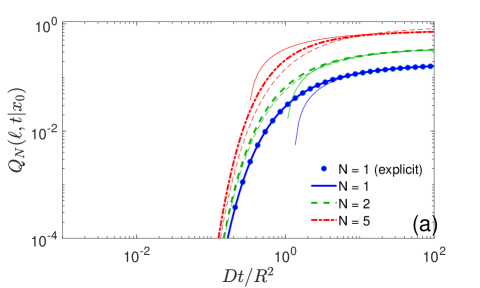
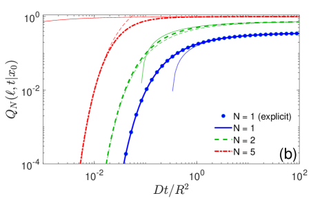
Figure 8: Cumulative distribution function $Q_{N}(\ell,t|\bm{x}_{0})$ of the first-crossing time ${\mathcal{T}}_{\ell,N}$ for $N$ particles diffusing in the exterior of a ball of radius $R=1$, with $\ell=1$, $D=1$, $|\bm{x}_{0}|=2$ (a) and $|\bm{x}_{0}|=1$ (b). Symbols present the explicit form (96) for a single particle, whereas thick lines show the numerical integration in Eq. (118). Thin lines indicate the long-time asymptotic relation (29), while thin dashed lines present the short-time behavior in Eq. (25) for $|\bm{x}_{0}|=2$ and Eq. (26) for $|\bm{x}_{0}|=1$, respectively.

Figure 2 illustrated the probability density $U_{N}(\ell,t|r_{0})$ and its asymptotic behavior for $\ell/R=1$. To provide a complementary view onto the properties of the first-crossing time, we also present the cumulative distribution function $Q_{N}(\ell,t|r_{0})$ on Fig. 8. As discussed previously, when the particles are released on the stock region, the stock depletion occurs much faster when $N$ increases.

For comparison, we also consider a smaller threshold $\ell/R=0.1$, for which the probability density $U_{N}(t,\ell|r_{0})$ is shown in Fig. 9. As previously, the behavior strongly depends on whether the particles start on the stock region (or close to it) or not. In the former case ($r_{0}=R$), the maximum of the probability density for $\ell/R=0.1$ is further shifted to smaller times, as expected. Note also that $U_{N}(\ell,t|r_{0})$ for $N=5$ exhibits a transitory regime at intermediate times with a rapid decay, so that the long-time behavior in Eq. (112), which remains correct, is not much useful here, as it describes the probability density of very small amplitude. In turn, for $r_{0}=2R$, the three curves on Fig. 9(a) resemble those on Fig. 2(a), because the limiting factor here is finding the stock region. In particular, setting $\ell=0$, one would get the probability density of the fastest first-passage time to the perfectly absorbing target Weiss83 ; Basnayake19 ; Lawley20 ; Lawley20b ; Lawley20c ; Grebenkov20d .

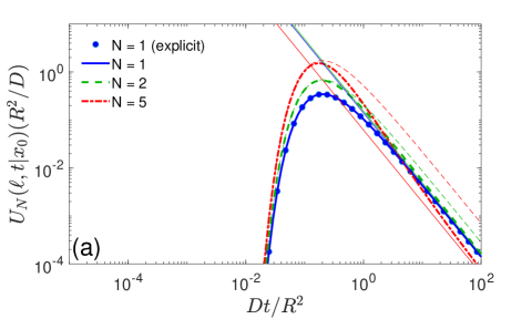
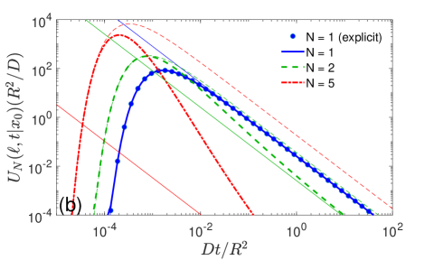
Figure 9: Probability density function $U_{N}(\ell,t|\bm{x}_{0})$ of the first-crossing time for $N$ particles diffusing in the exterior of a ball of radius $R=1$, with $\ell=0.1$, $D=1$, $|\bm{x}_{0}|=2$ (a) and $|\bm{x}_{0}|=1$ (b). Symbols present the explicit form (34) for a single particle, whereas thick lines show the numerical integration in Eq. (109). Thin lines indicate the long-time asymptotic relation (112), while thin dashed lines present the short-time behavior in Eq. (22) for $|\bm{x}_{0}|=2$ and Eq. (24) for $|\bm{x}_{0}|=1$.

Appendix C Numerical computation

As a numerical computation of the inverse Laplace transform may be unstable, it is convenient to replace the Laplace transform by the Fourier transform. This is equivalent to replacing the generating function ${\mathbb{E}}_{\bm{x}_{0}}\{e^{-q\ell_{t}}\}$ of $\ell_{t}$ by its characteristic function ${\mathbb{E}}_{\bm{x}_{0}}\{e^{iq\ell_{t}}\}$. In this way, we get

$$\rho_{N}(\ell,t|\bm{x}_{0}) =\int\limits_{-\infty}^{\infty}\frac{dq}{2\pi}e^{-iq\ell}\,{\mathbb{E}}_{\bm{x}_{0}}\{e^{iq\ell_{t}}\}$$

$$=\int\limits_{-\infty}^{\infty}\frac{dq}{2\pi}e^{-iq\ell}\,\bigl{(}{\mathbb{E}}_{\bm{x}_{0}}\{e^{iq\ell_{t}^{1}}\}\bigr{)}^{N}$$

$$=\int\limits_{-\infty}^{\infty}\frac{dq}{2\pi}e^{-iq\ell}\,\bigl{(}S_{-iq}(t|\bm{x}_{0})\bigr{)}^{N}.$$

Since the survival probability $S_{\infty}(t|\bm{x}_{0})$ is strictly positive for any $\bm{x}_{0}\notin\Gamma$, the total boundary local time $\ell_{t}$ can be zero with a finite probability $[S_{\infty}(t|\bm{x}_{0})]^{N}$, and it is convenient to subtract the contribution of this atom in the probability measure explicitly, so that

$$\rho_{N}(\ell,t|\bm{x}_{0})=\bigl{(}S_{\infty}(t|\bm{x}_{0})\bigr{)}^{N}\delta(\ell)$$ (114)

$$\quad+\int\limits_{-\infty}^{\infty}\frac{dq}{2\pi}e^{-iq\ell}\,\biggl{[}\bigl{(}S_{-iq}(t|\bm{x}_{0})\bigr{)}^{N}-\bigl{(}S_{\infty}(t|\bm{x}_{0})\bigr{)}^{N}\biggr{]},$$

where $\delta(\ell)$ is the Dirac distribution. The probabilistic interpretation of this relation is straightforward: as the total boundary local time remains $0$ until the first arrival of any of the particles onto the stock region, the random event $\ell_{t}=0$ (expressed by $\delta(\ell)$) has a strictly positive probability $\bigl{(}S_{\infty}(t|\bm{x}_{0})\bigr{)}^{N}$, i.e., the probability that none of $N$ particles has arrived onto the stock region up to time $t$. Since the diffusion equation (3) and the Robin boundary condition (4a) are linear, one has

$$S_{iq}(t|\bm{x}_{0})=S_{-iq}^{*}(t|\bm{x}_{0}),$$ (115)

where asterisk denotes the complex conjugate. As a consequence, one can rewrite Eq. (114) as

$$\rho_{N}(\ell,t|\bm{x}_{0})=\bigl{(}S_{\infty}(t|\bm{x}_{0})\bigr{)}^{N}\delta(\ell)$$ (116)

$$\quad+{\rm Re}\biggl{\{}\int\limits_{0}^{\infty}\frac{dq}{\pi}e^{iq\ell}\biggl{[}\bigl{(}S_{iq}(t|\bm{x}_{0})\bigr{)}^{N}-\bigl{(}S_{\infty}(t|\bm{x}_{0})\bigr{)}^{N}\biggr{]}\biggr{\}}.$$

Similarly, the probability density $U_{N}(\ell,t|\bm{x}_{0})$ and the cumulative distribution function $Q_{N}(\ell,t|\bm{x}_{0})$ can be written in the Fourier form as

$$U_{N}(\ell,t|\bm{x}_{0})={\rm Re}\biggl{\{}\int\limits_{0}^{\infty}\frac{dq}{\pi}\,\frac{e^{iq\ell}}{iq}\,\biggl{(}-\partial_{t}[S_{iq}(t|\bm{x}_{0})]^{N}\biggr{)}\biggr{\}}$$ (117)

and

$$Q_{N}(\ell,t|\bm{x}_{0})={\rm Re}\biggl{\{}\int\limits_{0}^{\infty}\frac{dq}{\pi}\,\frac{e^{iq\ell}}{iq}\,\biggl{(}[S_{iq}(t|\bm{x}_{0})]^{N}-1\biggr{)}\biggr{\}}.$$ (118)

References

- (1) M. Mangel and J. H. Beder, Search and Stock Depletion: Theory and Applications, Can. J. Fish Aquat. Sci. 42, 150-163 (1985).
- (2) Y. Wada, L. P. H. van Beek, C. M. van Kempen, J. W. T. M. Reckman, S. Vasak, and M. F. P. Bierkens, Global depletion of groundwater resources, Geophys. Res. Lett. 37, L20402 (2010).
- (3) R. Dirzo, H. S. Young, M. Galetti, G. Ceballos, N. J. B. Isaac, B. Collen, Defaunation in the Anthropocene, Science 345, 401-406 (2014).
- (4) O. Bénichou and S. Redner, Depletion-Controlled Starvation of a Diffusing Forager, Phys. Rev. Lett. 113, 238101 (2014).
- (5) M. Chupeau, O. Bénichou, and S. Redner, Universality classes of foraging with resource renewal, Phys. Rev. E 93, 032403 (2016).
- (6) O. Bénichou, M. Chupeau, and S. Redner, Role of depletion on the dynamics of a diffusing forager, J. Phys. A: Math. Theor. 49, 394003 (2016).
- (7) M. Chupeau, O. Bénichou, and S. Redner, Search in patchy media: Exploitation-exploration tradeoff, Phys. Rev. E 95, 012157 (2017).
- (8) U. Bhat, S. Redner, and O. Bénichou, Does greed help a forager survive? Phys. Rev. E 95, 062119 (2017).
- (9) O. Bénichou, U. Bhat, P. L. Krapivsky, and S. Redner, Optimally frugal foraging, Phys. Rev. E 97, 022110 (2018).
- (10) G. M. Viswanathan, M. G. E. da Luz, E. P. Raposo, and H. E. Stanley, The Physics of Foraging (Cambridge University Press, Cambridge, 2011).
- (11) G. M. Viswanathan, S. V. Buldyrev, S. Havlin, M. G. E. da Luz, E. P. Raposo, and H. E. Stanley, Optimizing the success of random searches, Nature 401, 911 (1999).
- (12) O. Bénichou, C. Loverdo, M. Moreau, and R. Voituriez, Intermittent search strategies, Rev. Mod. Phys. 83, 81-130 (2011).
- (13) T. Gueudré, A. Dobrinevski, and J.-P. Bouchaud, Explore or Exploit: A Generic Model and an Exactly Solvable Case, Phys. Rev. Lett. 112, 050602 (2014).
- (14) R. H. Fitts, Cellular mechanisms of muscle fatigue, Physiol. Rev. 74, 49-94 (1994).
- (15) A. B. Parekh and R. Penner, Store depletion and calcium influx, Physiol. Rev. 77, 901-930 (1997).
- (16) H. C. Ha and S. H. Snyde, Poly(ADP-ribose) polymerase is a mediator of necroticcell death by ATP depletion, Proc. Nat. Acad. Sci. U.S.A. 96, 13978-13982 (1999).
- (17) D. E. Clapham, Calcium Signaling, Cell 131, 1047-1058 (2007).
- (18) F. Spitzer, Principles of Random Walk (Springer-Verlag, New York, 1976).
- (19) S. Condamin, O. Bénichou, and M. Moreau, First-exit times and residence times for discrete random walks on finite lattices, Phys. Rev. E 72, 016127 (2005).
- (20) S. Condamin, V. Tejedor, and O. Bénichou, Occupation times of random walks in confined geometries: From random trap model to diffusion-limited reactions, Phys. Rev. E 76, 050102R (2007).
- (21) D. A. Darling and M. Kac, On Occupation Times of the Markoff Processes, Trans. Am. Math. Soc. 84, 444-458 (1957).
- (22) D. Ray, Sojourn times of diffusion processes, Illinois J. Math. 7, 615 (1963).
- (23) F. B. Knight, Random walks and a sojourn density process of Brownian motion, Trans. Amer. Math. Soc. 109, 56-86 (1963).
- (24) N. Agmon, Residence times in diffusion processes, J. Chem. Phys. 81, 3644 (1984).
- (25) A. M. Berezhkovskii, V. Zaloj, and N. Agmon, Residence time distribution of a Brownian particle, Phys. Rev. E 57, 3937 (1998).
- (26) A. Dhar and S. N. Majumdar, Residence time distribution for a class of Gaussian Markov processes, Phys. Rev. E 59, 6413 (1999).
- (27) S. B. Yuste and L. Acedo, Order statistics of the trapping problem, Phys. Rev. E 64, 061107 (2001).
- (28) C. Godrèche and J. M. Luck, Statistics of the Occupation Time of Renewal Processes, J. Stat. Phys. 104, 489 (2001).
- (29) S. N. Majumdar and A. Comtet, Local and Occupation Time of a Particle Diffusing in a Random Medium, Phys. Rev. Lett. 89, 060601 (2002).
- (30) O. Bénichou, M. Coppey, J. Klafter, M. Moreau, and G. Oshanin, On the joint residence time of N independent two-dimensional Brownian motions, J. Phys. A.: Math. Gen. 36, 7225-7231 (2003).
- (31) S. Burov and E. Barkai, Occupation Time Statistics in the Quenched Trap Model, Phys. Rev. Lett. 98, 250601 (2007).
- (32) S. Burov and E. Barkai, Residence Time Statistics for N Renewal Processes, Phys. Rev. Lett. 107, 170601 (2011).
- (33) D. S. Grebenkov, Residence times and other functionals of reflected Brownian motion, Phys. Rev. E 76, 041139 (2007).
- (34) P. Lévy, Processus Stochastiques et Mouvement Brownien (Paris, Gauthier-Villard, 1965).
- (35) K. Ito and H. P. McKean, Diffusion Processes and Their Sample Paths (Springer-Verlag, Berlin, 1965).
- (36) D. S. Grebenkov, Probability distribution of the boundary local time of reflected Brownian motion in Euclidean domains, Phys. Rev. E 100, 062110 (2019).
- (37) D. S. Grebenkov, Statistics of boundary encounters by a particle diffusing outside a compact planar domain, J. Phys. A.: Math. Theor. 54, 015003 (2021).
- (38) G. H. Weiss, K. E. Shuler, and K. Lindenberg, Order Statistics for First Passage Times in Diffusion Processes, J. Stat. Phys. 31, 255-278 (1983).
- (39) K. Basnayake, Z. Schuss, and D. Holcman, Asymptotic formulas for extreme statistics of escape times in 1, 2 and 3-dimensions, J. Nonlinear Sci. 29, 461-499 (2019).
- (40) S. D. Lawley and J. B. Madrid, A probabilistic approach to extreme statistics of Brownian escape times in dimensions 1, 2, and 3, J. Nonlin. Sci. 30, 1207-1227 (2020).
- (41) S. D. Lawley, Universal Formula for Extreme First Passage Statistics of Diffusion, Phys. Rev. E 101, 012413 (2020).
- (42) S. D. Lawley, Distribution of extreme first passage times of diffusion, J. Math. Biol. 80, 2301-2325 (2020).
- (43) A. J. Bray, S. Majumdar, and G. Schehr, Persistence and First-Passage Properties in Non-equilibrium Systems, Adv. Phys. 62, 225-361 (2013).
- (44) S. N. Majumdar, A. Pal, and G. Schehr, Extreme value statistics of correlated random variables: a pedagogical review, Phys. Rep. 840, 1-32 (2020).
- (45) D. S. Grebenkov, R. Metzler, and G. Oshanin, From single-particle stochastic kinetics to macroscopic reaction rates: fastest first-passage time of N random walkers, New J. Phys. 22, 103004 (2020).
- (46) D. S. Grebenkov, Paradigm shift in diffusion-mediated surface phenomena, Phys. Rev. Lett. 125, 078102 (2020).
- (47) F. C. Collins and G. E. Kimball, Diffusion-controlled reaction rates, J. Coll. Sci. 4, 425 (1949).
- (48) H. Sano and M. Tachiya, Partially diffusion-controlled recombination, J. Chem. Phys. 71, 1276-1282 (1979).
- (49) H. Sano and M. Tachiya, Theory of diffusion-controlled reactions on spherical surfaces and its application to reactions on micellar surfaces, J. Chem. Phys. 75, 2870-2878 (1981).
- (50) D. Shoup and A. Szabo, Role of diffusion in ligand binding to macromolecules and cell-bound receptors, Biophys. J. 40, 33-39 (1982).
- (51) R. Zwanzig, Diffusion-controlled ligand binding to spheres partially covered by receptors: an effective medium treatment, Proc. Natl. Acad. Sci. USA 87, 5856 (1990).
- (52) B. Sapoval, General Formulation of Laplacian Transfer Across Irregular Surfaces, Phys. Rev. Lett. 73, 3314-3317 (1994).
- (53) M. Filoche and B. Sapoval, Can One Hear the Shape of an Electrode? II. Theoretical Study of the Laplacian Transfer, Eur. Phys. J. B 9, 755-763 (1999).
- (54) B. Sapoval, M. Filoche, and E. Weibel, Smaller is better – but not too small: A physical scale for the design of the mammalian pulmonary acinus, Proc. Nat. Ac. Sci. USA 99, 10411-10416 (2002).
- (55) D. S. Grebenkov, M. Filoche, and B. Sapoval, Spectral Properties of the Brownian Self-Transport Operator, Eur. Phys. J. B 36, 221-231 (2003).
- (56) A. Berezhkovskii, Y. Makhnovskii, M. Monine, V. Zitserman, and S. Shvartsman, Boundary homogenization for trapping by patchy surfaces, J. Chem. Phys. 121, 11390 (2004).
- (57) D. S. Grebenkov, M. Filoche, B. Sapoval, and M. Felici, Diffusion-Reaction in Branched Structures: Theory and Application to the Lung Acinus, Phys. Rev. Lett. 94, 050602 (2005).
- (58) D. S. Grebenkov, M. Filoche, and B. Sapoval, Mathematical Basis for a General Theory of Laplacian Transport towards Irregular Interfaces, Phys. Rev. E 73, 021103 (2006).
- (59) S. D. Traytak and W. Price, Exact solution for anisotropic diffusion-controlled reactions with partially reflecting conditions, J. Chem. Phys. 127, 184508 (2007).
- (60) P. C. Bressloff, B. A. Earnshaw, and M. J. Ward, Diffusion of protein receptors on a cylindrical dendritic membrane with partially absorbing traps, SIAM J. Appl. Math. 68, 1223-1246 (2008).
- (61) S. D. Lawley and J. P. Keener, A New Derivation of Robin Boundary Conditions through Homogenization of a Stochastically Switching Boundary, SIAM J. Appl. Dyn. Sys. 14, 1845-1867 (2015).
- (62) M. Galanti, D. Fanelli, S. D. Traytak, and F. Piazza, Theory of diffusion-influenced reactions in complex geometries, Phys. Chem. Chem. Phys. 18, 15950-15954 (2016).
- (63) A. E. Lindsay, A. J. Bernoff, and M. J. Ward, First Passage Statistics for the Capture of a Brownian Particle by a Structured Spherical Target with Multiple Surface Traps, Multiscale Model. Simul. 15, 74-109 (2017).
- (64) D. S. Grebenkov and G. Oshanin, Diffusive escape through a narrow opening: new insights into a classic problem, Phys. Chem. Chem. Phys. 19, 2723-2739 (2017).
- (65) A. Bernoff, A. Lindsay, and D. Schmidt, Boundary Homogenization and Capture Time Distributions of Semipermeable Membranes with Periodic Patterns of Reactive Sites, Multiscale Model. Simul. 16, 1411-1447 (2018).
- (66) D. S. Grebenkov and S. Traytak, Semi-analytical computation of Laplacian Green functions in three-dimensional domains with disconnected spherical boundaries, J. Comput. Phys. 379, 91-117 (2019).
- (67) T. Guérin, M. Dolgushev, O. Bénichou, and R. Voituriez, Universal kinetics of imperfect reactions in confinement, Commun. Chem. 4, 157 (2021).
- (68) D. S. Grebenkov, Joint distribution of multiple boundary local times and related first-passage time problems, J. Stat. Mech. 103205 (2020).
- (69) S. Redner, A Guide to First Passage Processes (Cambridge: Cambridge University press, 2001).
- (70) N. Levernier, M. Dolgushev, O. Bénichou, R. Voituriez, and T. Guérin, Survival probability of stochastic processes beyond persistence exponents, Nat. Comm 10, 2990 (2019).
- (71) R. F. Kayser and J. B. Hubbard, Diffusion in a Medium with a Random Distribution of Static Traps, Phys. Rev. Lett. 51, 79 (1983).
- (72) R. F. Kayser and J. B. Hubbard, Reaction diffusion in a medium containing a random distribution of nonoverlapping traps, J. Chem. Phys. 80, 1127 (1984).
- (73) P. Levitz, M. Zinsmeister, P. Davidson, D. Constantin, and O. Poncelet, Intermittent Brownian dynamics over a rigid strand: Heavily tailed relocation statistics, Phys. Rev. E 78, 030102(R) (2008).
- (74) D. S. Grebenkov, Surface Hopping Propagator: An Alternative Approach to Diffusion-Influenced Reactions, Phys. Rev. E 102, 032125 (2020).
- (75) M. Smoluchowski, Versuch einer Mathematischen Theorie der Koagulations Kinetic Kolloider Lösungen, Z. Phys. Chem. 92U, 129-168 (1917).
- (76) M. R. Evans and S. N. Majumdar, Diffusion with Stochastic Resetting, Phys. Rev. Lett. 106, 160601 (2011).
- (77) A. V. Chechkin and I. M. Sokolov, Random Search with Resetting: A Unified Renewal Approach, Phys. Rev. Lett. 121, 050601 (2018).
- (78) M. R. Evans, S. N. Majumdar, and G. Schehr, Stochastic resetting and applications, J. Phys. A: Math. Theor. 53, 193001 (2020).
- (79) B. Meerson and S. Redner, Mortality, Redundancy, and Diversity in Stochastic Search, Phys. Rev. Lett. 114, 198101 (2015).
- (80) D. S. Grebenkov and J.-F. Rupprecht, The escape problem for mortal walkers, J. Chem. Phys. 146, 084106 (2017).
- (81) D. S. Grebenkov, An encounter-based approach for restricted diffusion with a gradient drift, J. Phys. A: Math. Theor. 55, 045203 (2022).
- (82) A. Godec and R. Metzler, First passage time statistics for two-channel diffusion, J. Phys. A: Math. Theor. 50, 084001 (2017).
- (83) Y. Lanoiselée, N. Moutal, and D. S. Grebenkov, Diffusion-limited reactions in dynamic heterogeneous media, Nature Commun. 9, 4398 (2018).
- (84) V. Sposini, A. V. Chechkin, and R. Metzler, First passage statistics for diffusing diffusivity, J. Phys. A: Math. Theor. 52, 04LT01 (2019).
- (85) D. S. Grebenkov, A unifying approach to first-passage time distributions in diffusing diffusivity and switching diffusion models, J. Phys. A: Math. Theor. 52, 174001 (2019).
- (86) A. N. Borodin and P. Salminen, Handbook of Brownian Motion: Facts and Formulae (Birkhauser Verlag, Basel-Boston-Berlin, 1996).
- (87) B. Sapoval, J. S. Andrade Jr, A. Baldassari, A. Desolneux, F. Devreux, M. Filoche, D. S. Grebenkov, S. Russ, New Simple Properties of a Few Irregular Systems, Physica A 357, 1-17 (2005).
- (88) D. S. Grebenkov, Analytical representations of the spread harmonic measure, Phys. Rev. E 91, 052108 (2015).
- (89) J. Madrid and S. D. Lawley, Competition between slow and fast regimes for extreme first passage times of diffusion, J. Phys. A: Math. Theor. 53, 335002 (2020).
- (90) D. S. Grebenkov, R. Metzler, and G. Oshanin, Strong defocusing of molecular reaction times results from an interplay of geometry and reaction control, Commun. Chem. 1, 96 (2018).