A Deep Learning Approach to Dst Index Prediction

Abstract

The disturbance storm time (Dst) index is an important and useful measurement in space weather research. It has been used to characterize the size and intensity of a geomagnetic storm. A negative Dst value means that the Earth’s magnetic field is weakened, which happens during storms. In this paper, we present a novel deep learning method, called the Dst Transformer, to perform short-term, 1-6 hour ahead, forecasting of the Dst index based on the solar wind parameters provided by the NASA Space Science Data Coordinated Archive. The Dst Transformer combines a multi-head attention layer with Bayesian inference, which is capable of quantifying both aleatoric uncertainty and epistemic uncertainty when making Dst predictions. Experimental results show that the proposed Dst Transformer outperforms related machine learning methods in terms of the root mean square error and R-squared. Furthermore, the Dst Transformer can produce both data and model uncertainty quantification results, which can not be done by the existing methods. To our knowledge, this is the first time that Bayesian deep learning has been used for Dst index forecasting.

1 Introduction

Geomagnetic activities have significant impact on Earth. They can disturb or damage telephone systems, power grid transmission systems and space satellites. Geomagnetic activity modeling and forecasting has therefore been an important subject in space weather research. The main source of geomagnetic activity is solar activity. The solar wind, which is a stream of charged particles released from the atmosphere of the Sun, is considered as the medium through which the Sun exerts influence on Earth. As a consequence, solar wind parameters such as the interplanetary magnetic field (IMF), total electric field, solar wind speed and plasma temperature are often used to model geomagnetic activities and forecast geomagnetic indices.

The disturbance storm time (Dst) index is an important geomagnetic index. It has been used to characterize the size and intensity of a geomagnetic storm. A negative Dst value means that the Earth’s magnetic field is weakened, which happens during storms. A storm is considered moderate when Dst is greater than $-50$ nT, intense when Dst is between $-50$ nT and $-250$ nT, or super when Dst is less than $-250$ nT (Loewe and Prölss, 1997; Gruet et al., 2018).

Many techniques have been developed to model and forecast the Dst index. For example, Burton, McPherron, and Russell (1975) adopted differential equations to model the Dst index. The authors used solar wind parameters as the source of differential equations in their model. Gleisner, Lundstedt, and Wintoft (1996) created the first Dst prediction model by employing a time-delay artificial neural network (ANN) with solar wind parameters as input. The authors performed 1-6 hour ahead predictions for the Dst index forecasting. Bala and Reiff (2012) discussed another strategy by combining physical models and ANNs, along with parameters such as the solar wind velocity, IMF magnitude, and IMF clock angle. Lazzús et al. (2017) employed a particle swarm optimization technique to train ANN connection weights to improve the accuracy of Dst index predictions.

The above approaches mainly focused on single point predictions. Chandorkar, Camporeale, and Wing (2017) extended the above approaches by considering probabilistic forecasting of the Dst index. The authors used Gaussian processes (GP) to build autoregressive models to estimate Dst 1 hour ahead based on past Dst values, as well as the solar wind velocity and the IMF Bz component. Their technique generated a predictive distribution instead of single point predictions. However, the mean values of the forecasts are not as accurate as the forecasts produced by ANNs. To improve GP’s poor point prediction performance, Gruet et al. (2018) built a Dst index prediction model by combining GP with a long short-term memory (LSTM) network.

In this paper, we present a novel Bayesian deep learning approach for performing short-term, 1-6 hour ahead, predictions of the Dst index. Our approach, called the Dst Transformer and denoted by DSTT, combines a multi-head attention layer with Bayesian inference capable of handling both aleatoric uncertainty and epistemic uncertainty. Aleatoric uncertainty, also known as data uncertainty, measures the noise inherent in data. Epistemic uncertainty, also known as model uncertainty, measures the uncertainty in the parameters of a model (Kendall and Gal, 2017). Thus, our work extends the aforementioned GP-based probabilistic forecasts, which can only handle model uncertainty, to quantify both data and model uncertainties through Bayesian inference. It is worth noting that Bayesian deep learning has also been used to mine solar images (Jiang et al., 2021). However, Dst values are time series data, not image data, and hence the architecture of our Dst Transformer is totally different from the model architecture developed by Jiang et al. (2021).

The contributions of our work are summarized below.

• Our DSTT model is the first to utilize the Transformer network to forecast the Dst index for a short-term period (i.e., 1-6 hours ahead).

• This is the first study in which both data and model uncertainties are quantified when performing Dst index forecasting.

• Our DSTT model outperforms closely comparable machine learning methods for short-term Dst index forecasting, as evidenced by performance metrics including the root mean square error (RMSE) and R-squared (R²).

2 Data

2.1 Data Source

The Dst index measurements used in this study are provided by the NASA Space Science Data Coordinated Archive. The data source provides other widely accessed data that are frequently used in solar wind analysis. The data source is being periodically updated with Advanced Composition Explorer (ACE). We used the Dst index data in the time period between January 1, 2010 and November 15, 2021. We selected the time resolution of the hourly average for the Dst index. Following Lethy et al. (2018), we considered seven solar wind parameters, namely the interplanetary magnetic field (IMF), magnetic field Bz component, plasma temperature, proton density, plasma speed, flow pressure, and electric field. The total number of records in our dataset is 104,080. The Dst index values in the dataset range from 77 nT to $-223$ nT.

2.2 Data Labeling

We divided our dataset into two parts: training set and test set. The training set contains 102,976 records from January 1, 2010 to September 30, 2021. The test set contains 1104 records from October 1, 2021 to November 15, 2021. The training set and test set are disjoint. The records are labeled as follows. Let $t$ be a time point of interest and let $w$ be the time window ahead of $t$, where $w$ ranges from 1 to 6 hours for the short-term Dst forecasting studied here. The label of the record at time point $t$ is defined as the Dst index value at time point $t+w$ for $w$-hour-ahead forecasting. Each record in the training set has eight values including the seven solar wind parameter values and the label of the training record. Each record in the test set contains only the seven solar wind parameter values; the label of each testing record in the test set will be predicted by our DSTT model.

3 Proposed Method

3.1 Architecture of the DSTT Model

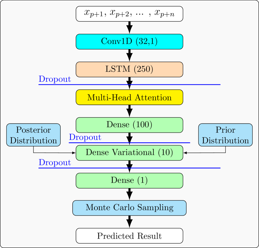
Figure 1: Architecture of our Dst Transformer (DSTT).

Figure 1 presents the architecture of our DSTT model. DSTT is created using the tensorflow keras framework. We add multiple layers to DSTT to enhance its performance and improve its learning capability. The model accepts as input non-overlapping sequences of records ${x_{p+1}}$, ${x_{p+2}}$, $\ldots$ , ${x_{p+n}}$, where $n$ is set to 1024 in our study. Each sequence is passed to a one-dimensional convolution neural network (Conv1D) with 32 kernels where the size of each kernel is 1. Conv1D is well suited for sequential data; it learns patterns from the input data sequence and passes them to a long short-term memory (LSTM) layer that is configured with 250 LSTM units. Combining Conv1D and LSTM layers has shown significant improvement in performance when dealing with sequential data such as time series (Abduallah et al., 2021; Faghihi and Kalantarpour, 2021). LSTM hands the learned patterns down to a multi-head attention layer (Vaswani et al., 2017). The multi-head attention layer provides transformation on the sequential input of values to obtain distinct metrics of size $h$. Here, $h$ is the number of attention heads that is set to 3 and the size of each attention head is also set to 3 because a number greater than 3 caused overhead and less than 3 caused performance degradation. The other parameters are left with their default values.

Furthermore, we add custom attention to instruct the layers to focus and pay more attention to critical information of the input data sequence and capture the correlation between the input and output by computing the weighted sum of the data sequence. In addition, we add a dense variational layer (DVL) (Tran et al., 2019) with 10 neurons that uses variational inference (Blei, Kucukelbir, and McAuliffe, 2016) to approximate the posterior distribution over the model weights. DVL is similar to a regular dense layer, but requires two input functions that define the prior and posterior distributions over the model weights. DVL allows our DSTT model to represent the weights by a distribution instead of estimated points.

DSTT also includes multiple dense and dropout layers. Each dense layer is strongly connected with its preceding layer where every neuron in the dense layer is connected with every neuron in the preceding layer. Each dropout layer instructs the DSTT model to randomly drop a percentage of its hidden neurons throughout the training phase to avoid over-fitting of training data.

3.2 Uncertainty Quantification

Quantifying uncertainty with a deep learning model has been used in many applications such as medical image processing (Kwon et al., 2020), computer vision (Kendall and Gal, 2017), space weather (Gruet et al., 2018) and solar physics (Jiang et al., 2021). Our proposed DSTT model contains a dense variational layer (DVL) that provides a weight distribution and multiple dropout layers that drop or turn off certain number of neurons during the training phase. Dropout is mainly used in deep learning to prevent over-fitting, where a trained model can be generalized for prediction instead of fitting exactly against its training data. With the dropout, the model’s internal architecture is slightly different each time the neurons are dropped. This is an important behavior to the Monte Carlo (MC) class of algorithms that depends on random sampling and provides useful information (Gal and Ghahramani, 2016). We use this technique to introduce a distribution interval of predicted values as demonstrated in Section “Experiments and Results.”

Specifically, to quantify the uncertainty with our DSTT model, we use a prior probability, $P(W)$, over the model’s weights, $W$. During training, the seven solar wind parameter values and Dst index values, collectively referred to as $D$, are used to train the model. According to Bayes’ theorem,

$$P(W|D)=\frac{P(D|W)\times P(W)}{P(D)}.$$ (1)

Computation of the exact posterior probability, $P(W|D)$, is intractable (Jiang et al., 2021), but we can use variational inference (Graves, 2011) to learn the variational distribution over the model’s weights parameterized by $\theta$, $q_{\theta}(W)$, by minimizing the Kullback–Leibler (KL) divergence of $q_{\theta}(W)$ and $P(W|D)$ (Blei, Kucukelbir, and McAuliffe, 2016). According to Gal and Ghahramani (2016), a network with a dropout provides variational approximation. To minimize the KL divergence, we use the dense variational layer (DVL) shown in Figure 1 and assign the KL weight to $1/N$ where $N$ is the size of the training set (Ling and Dai, 2012). We use the mean squared error (MSE) loss function and the adaptive moment estimation (Adam) optimizer (Goodfellow, Bengio, and Courville, 2016) with a learning rate of 0.0001 to train our model. Let $\hat{\theta}$ denote the optimized variational parameter obtained by training the model; we use $q_{\hat{\theta}}(W)$ to represent the optimized weight distribution.

During testing/prediction, our model utilizes the MC dropout sampling technique to produce probabilistic forecasting results, quantifying both aleatoric and epistemic uncertainties. Dropout is used to retrieve $K$ MC samples by processing the test data $K$ times (Gal and Ghahramani, 2016). (In the study presented here, $K$ is set to 100.) For each of the $K$ MC samples, a set of weights is randomly drawn from $q_{\hat{\theta}}(W)$. For each predicted Dst value, we get a mean and a variance over the $K$ samples. Following (Kwon et al., 2020; Jiang et al., 2021), we decompose the variance into aleatoric and epistemic uncertainties. The aleatoric uncertainty captures the inherent randomness of the predicted result, which comes from the input test data. On the other hand, the epistemic uncertainty comes from the variability of $W$, which accounts for the uncertainty in the model parameters (weights).

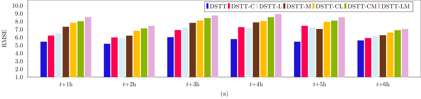
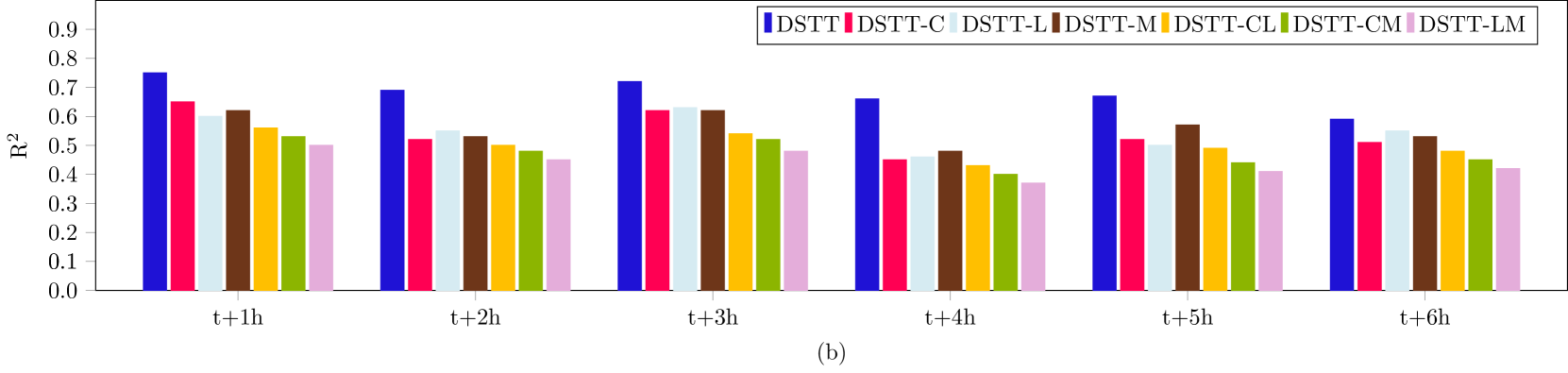
Figure 2: Results of the ablation study.

4 Experiments and Results

4.1 Performance Metrics

We conducted a series of experiments to evaluate our proposed DSTT model and compare it with closely related methods. The performance metrics used in our study are the root mean square error (RMSE) (Abduallah et al., 2021) and R-squared (R²).

RMSE is calculated as follows:

$$\mbox{RMSE}=\sqrt{\frac{1}{m}\sum_{i=1}^{m}({y_{i}}-\hat{y_{i}})^{2}},$$ (2)

where $m$ is the total number of testing records in the test set, $\hat{y_{i}}$ ($y_{i}$, respectively) represents the predicted Dst index value (observed Dst index value, respectively) at time point $i$. The smaller the RMSE, the more accurate a method is.

R² is calculated as follows:

$$\mbox{R\textsuperscript{2}}=1-\frac{\sum_{i}^{m}({y_{i}}-\hat{y_{i}})^{2}}{\sum_{i}^{m}({y_{i}}-\bar{y})^{2}},$$ (3)

where $\bar{y}$ is the mean of the observed Dst index values. The larger the R², the more accurate a method is.

4.2 Ablation Study

In this experiment, we performed ablation tests to analyze and evaluate the components of our DSTT model. We considered six subnets derived from DSTT: DSTT-C, DSTT-L, DSTT-M, DSTT-CL, DSTT-CM and DSTT-LM. DSTT-C (DSTT-L, DSTT-M, DSTT-CL, DSTT-CM, DSTT-LM, respectively) represents the subnet of DSTT in which we remove the Conv1D layer (LSTM layer, multi-head attention layer, Conv1D and LSTM layers, Conv1D and multi-head attention layers, LSTM and multi-head attention layers, respectively) while keeping the remaining components of the DSTT network. For comparison purposes, we turned off the uncertainty quantification mechanism in the seven models.

Figure 2 presents the RMSE and R² results of the seven models. The $t+w$h, $1\leq w\leq 6$, on the X-axis corresponds to the $w$-hour ahead predictions of the Dst index based on the testing records in the test set. It can be seen from Figure 2 that our proposed full network model, DSTT, achieves the best performance among the seven models. DSTT-C captures the temporal correlation from the input data but it does not learn additional patterns and properties to strengthen the relationship between data records. DSTT-L captures the properties from the data records but it lacks the temporal correlation information to deeply analyze the sequential information in the input data. DSTT-M captures both the temporal correlation and additional properties, but it does not provide transformation on the sequential inputs to obtain distinct metrics to further strengthen the correlation between the predicted and observed Dst values. Similarity, DSTT-CL, DSTT-CM, and DSTT-LM do not capture the combined patterns due to the removed layers. As a consequence, the six subnets achieve worse performance than DSTT. It can be seen from Figure 2 that removing two layers yields worse results than removing one layer only. DSTT-LM yields the worst results, indicating the importance of including the LSTM and multi-head attention layers. The results based on RMSE and R² are consistent. In subsequent experiments, we used DSTT due to its best performance among the seven models.

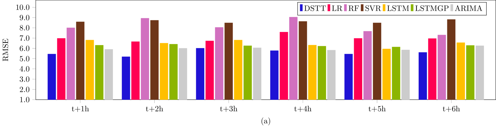
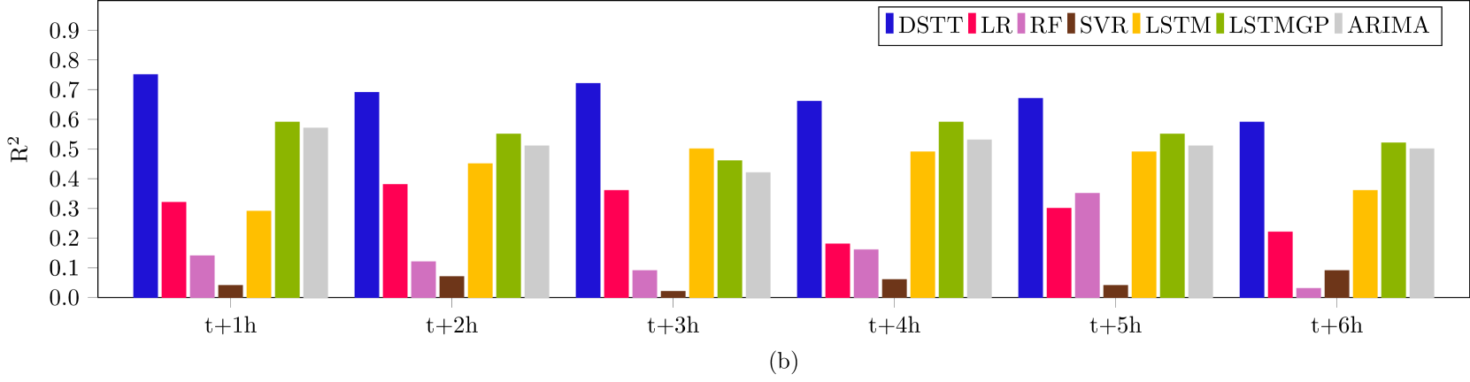
Figure 3: Performance comparison of seven Dst forecasting methods.

4.3 Comparison with Related Methods

In this experiment, we compared the Dst Transformer (DSTT) with six closely related machine learning methods including linear regression (LR), random forests (RF), support vector regression (SVR), auto regressive integrated moving average (ARIMA) (Tyass et al., 2022), long short-term memory (LSTM), and the method developed by Gruet et al. (2018), which combines LSTM with Gaussian processes (GP) and is denoted by LSTMGP. Because the six related methods do not have the ability to quantify both data and model uncertainties, we turned off the uncertainty quantification mechanism in our DSTT model when performing this experiment.

Figure 3 presents the RMSE and R² results of the seven methods: DSTT, LR, RF, SVR, ARIMA, LSTM and LSTMGP. It can be seen from the figure that DSTT achieves the best performance, producing the most accurate predictions, among the seven methods in terms of both RMSE and R². The deep learning methods including DSTT, LSTM and LSTMGP as well as ARIMA mostly perform better than the traditional machine learning algorithms including RF, LR and SVR.

4.4 Uncertainty Quantification Results

Figure 4 shows uncertainty quantification results produced by our DSTT model on the test set. Due to space limitation, we only present the results obtained from 4-hour ahead predictions of the Dst index. In Figure 4, the orange lines represent observed values of the Dst index (ground truth) while the blue lines represent the predicted values of the Dst index. The light blue region in Figure 4(a) represents aleatoric uncertainty (data uncertainty). The light gray region in Figure 4(b) represents epistemic uncertainty (model uncertainty).

It can be seen from Figure 4 that the blue lines are reasonably close to the orange lines, indicating the good performance of our DSTT model, which is consistent with the results in Figure 3. Figure 4 also shows that the light gray region is much smaller than the light blue region, indicating that the model uncertainties are much smaller than the data uncertainties. Thus, the uncertainty in the predicted result is mainly due to the noise in the input test data. Similar results were obtained from other $w$-hour, $1\leq w\leq 6$, $w\not=4$, ahead predictions of the Dst index. We note that when $w$ is longer than 4, the prediction performance starts to degrade. This is understandable given that we are trying to predict a Dst index value that is farther away from the input test record.

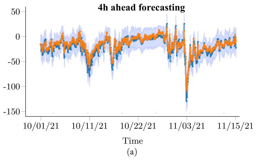
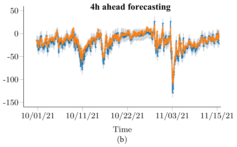
Figure 4: Uncertainty quantification results produced by our Dst Transformer (DSTT).

5 Discussion and Conclusions

The disturbance storm time (Dst) index is an important and useful measurement in space weather research, which is used to understand the severity of a geomagnetic storm. The Dst index is also known as the measure of the decrease in the Earth’s magnetic field. In this paper, we present a novel deep learning model, called the Dst Transformer or DSTT, to perform short-term, 1-6 hour ahead predictions of the Dst index. Our empirical study demonstrated the good performance of the Dst Transformer and its superiority over related methods.

Our experiments were based on the data collected in the period between January 1, 2010 and November 15, 2021. The training set contained hourly records from January 1, 2010 to September 30, 2021. The test set contained hourly records from October 1, 2021 to November 15, 2021. To avoid bias in our findings, we performed additional experiments using 10-fold cross validation (CV). For the CV tests, we used the original data set described above and another data set ranging from November 28, 1963 to March 1, 2022 that has 510,696 records. In addition, we generated synthetic data with up to 1.2 million records to further assess the performance and stability of our DSTT model. With the 10-fold CV tests, the data was divided into 10 approximately equal partitions or folds. The sequential order of the data in each fold was maintained. In each run, one fold was used for testing and the other nine folds together were used for training. There were 10 folds and hence 10 runs. We computed the performance metrics including RMSE and R² for each method studied in the paper in each run. The means and standard deviations of the metric values over the 10 runs were calculated and recorded. Results from the 10-fold CV tests were consistent with those reported in the paper. Thus we conclude that the proposed Dst Transformer (DSTT) is a feasible machine learning method for short-term, 1-6 hour ahead predictions of the Dst index. Furthermore, our DST Transformer can quantify both data and model uncertainties in making the predictions, which can not be done by the related methods.

Our work focuses on short-term predictions of the Dst index by utilizing solar wind parameters. These solar wind parameters are collected by instruments near Earth and are suited for short-term predictions of the geomagnetic storms near Earth (Gruet et al., 2018; Lethy et al., 2018). When using the solar wind parameters to perform long-term (e.g., 3-day ahead) predictions of the Dst index, the accuracy is low. In future work, we plan to perform long-term predictions of the Dst index by utilizing solar data collected by instruments near the Sun. The solar data reflects solar activity, which is the source of geomagnetic activity. We plan to extend the Bayesian deep learning method described here to mine the solar data for performing long-term Dst index forecasts.

6 Acknowledgments

We acknowledge the use of NASA/GSFC’s Space Physics Data Facility’s OMNIWeb service and OMNI data.

References

- Abduallah et al. (2021) Abduallah, Y.; Wang, J. T. L.; Shen, Y.; Alobaid, K. A.; Criscuoli, S.; and Wang, H. 2021. Reconstruction of total solar irradiance by deep learning. The International FLAIRS Conference Proceedings 34.
- Bala and Reiff (2012) Bala, R., and Reiff, P. 2012. Improvements in short-term forecasting of geomagnetic activity. Space Weather 10(6).
- Blei, Kucukelbir, and McAuliffe (2016) Blei, D. M.; Kucukelbir, A.; and McAuliffe, J. D. 2016. Variational inference: A review for statisticians. Journal of the American Statistical Association 112:859 – 877.
- Burton, McPherron, and Russell (1975) Burton, R. K.; McPherron, R. L.; and Russell, C. T. 1975. An empirical relationship between interplanetary conditions and Dst. Journal of Geophysical Research (1896-1977) 80(31):4204–4214.
- Chandorkar, Camporeale, and Wing (2017) Chandorkar, M.; Camporeale, E.; and Wing, S. 2017. Probabilistic forecasting of the disturbance storm time index: An autoregressive Gaussian process approach. Space Weather 15(8):1004–1019.
- Faghihi and Kalantarpour (2021) Faghihi, U., and Kalantarpour, C. 2021. Using deep learning algorithms to detect the success or failure of the Electroconvulsive Therapy (ECT) sessions. The International FLAIRS Conference Proceedings 34.
- Gal and Ghahramani (2016) Gal, Y., and Ghahramani, Z. 2016. Dropout as a Bayesian approximation: Representing model uncertainty in deep learning. In Proceedings of the 33rd International Conference on Machine Learning, 1050–1059.
- Gleisner, Lundstedt, and Wintoft (1996) Gleisner, H.; Lundstedt, H.; and Wintoft, P. 1996. Predicting geomagnetic storms from solar-wind data using time-delay neural networks. Annales Geophysicae 14:679–686.
- Goodfellow, Bengio, and Courville (2016) Goodfellow, I. J.; Bengio, Y.; and Courville, A. C. 2016. Deep Learning. MIT Press.
- Graves (2011) Graves, A. 2011. Practical variational inference for neural networks. In Shawe-Taylor, J.; Zemel, R.; Bartlett, P.; Pereira, F.; and Weinberger, K. Q., eds., Advances in Neural Information Processing Systems, volume 24.
- Gruet et al. (2018) Gruet, M. A.; Chandorkar, M.; Sicard, A.; and Camporeale, E. 2018. Multiple-hour-ahead forecast of the Dst index using a combination of long short-term memory neural network and Gaussian process. Space Weather 16(11):1882–1896.
- Jiang et al. (2021) Jiang, H.; Jing, J.; Wang, J.; Liu, C.; Li, Q.; Xu, Y.; Wang, J. T. L.; and Wang, H. 2021. Tracing H fibrils through Bayesian deep learning. The Astrophysical Journal Supplement Series 256(1):20.
- Kendall and Gal (2017) Kendall, A., and Gal, Y. 2017. What uncertainties do we need in Bayesian deep learning for computer vision? In Guyon, I.; Luxburg, U. V.; Bengio, S.; Wallach, H.; Fergus, R.; Vishwanathan, S.; and Garnett, R., eds., Advances in Neural Information Processing Systems, volume 30. Curran Associates, Inc.
- Kwon et al. (2020) Kwon, Y.; Won, J.-H.; Kim, B. J.; and Paik, M. C. 2020. Uncertainty quantification using Bayesian neural networks in classification: Application to biomedical image segmentation. Computational Statistics & Data Analysis 142:106816.
- Lazzús et al. (2017) Lazzús, J. A.; Vega, P.; Rojas, P.; and Salfate, I. 2017. Forecasting the Dst index using a swarm-optimized neural network. Space Weather 15(8):1068–1089.
- Lethy et al. (2018) Lethy, A.; El-Eraki, M. A.; Samy, A.; and Deebes, H. A. 2018. Prediction of the Dst index and analysis of its dependence on solar wind parameters using neural network. Space Weather 16(9):1277–1290.
- Ling and Dai (2012) Ling, Z.-H., and Dai, L.-R. 2012. Minimum Kullback-Leibler divergence parameter generation for HMM-based speech synthesis. IEEE Transactions on Audio, Speech, and Language Processing 20(5):1492–1502.
- Loewe and Prölss (1997) Loewe, C. A., and Prölss, G. W. 1997. Classification and mean behavior of magnetic storms. Journal of Geophysical Research: Space Physics 102(A7):14209–14213.
- Tran et al. (2019) Tran, D.; Dusenberry, M. W.; van der Wilk, M.; and Hafner, D. 2019. Bayesian Layers: A Module for Neural Network Uncertainty. Red Hook, NY, USA: Curran Associates Inc. 14660–14672.
- Tyass et al. (2022) Tyass, I.; Bellat, A.; Raihani, A.; Mansouri, K.; and Khalili, T. 2022. Wind speed prediction based on seasonal ARIMA model. In E3S Web of Conferences, volume 336 of E3S Web of Conferences, 00034.
- Vaswani et al. (2017) Vaswani, A.; Shazeer, N.; Parmar, N.; Uszkoreit, J.; Jones, L.; Gomez, A. N.; Kaiser, L.; and Polosukhin, I. 2017. Attention is all you need. In Guyon, I.; Luxburg, U. V.; Bengio, S.; Wallach, H.; Fergus, R.; Vishwanathan, S.; and Garnett, R., eds., Advances in Neural Information Processing Systems, volume 30. Curran Associates, Inc.