FAITH: Few-Shot Graph Classification with
Hierarchical Task Graphs
Abstract
Few-shot graph classification aims at predicting classes for graphs, given limited labeled graphs for each class. To tackle the bottleneck of label scarcity, recent works propose to incorporate few-shot learning frameworks for fast adaptations to graph classes with limited labeled graphs. Specifically, these works propose to accumulate meta-knowledge across diverse meta-training tasks, and then generalize such meta-knowledge to the target task with a disjoint label set. However, existing methods generally ignore task correlations among meta-training tasks while treating them independently. Nevertheless, such task correlations can advance the model generalization to the target task for better classification performance. On the other hand, it remains non-trivial to utilize task correlations due to the complex components in a large number of meta-training tasks. To deal with this, we propose a novel few-shot learning framework FAITH that captures task correlations via constructing a hierarchical task graph at different granularities. Then we further design a loss-based sampling strategy to select tasks with more correlated classes. Moreover, a task-specific classifier is proposed to utilize the learned task correlations for few-shot classification. Extensive experiments on four prevalent few-shot graph classification datasets demonstrate the superiority of FAITH over other state-of-the-art baselines.
1 INTRODUCTION
Graph classification aims at predicting classes for graph samples, and many real-world problems can be formulated under this scenario Xu et al. (2019); Ma et al. (2020). As an example, in the task of molecular property predictions Chauhan et al. (2020), each molecule is represented as a graph, and molecular properties are regarded as graph labels. Generally, Graph Neural Networks (GNNS) Kipf and Welling (2017); Veličković et al. (2018); Xu et al. (2018) have achieved promising performance in molecular property predictions. However, their performance drops significantly in the few-shot scenario Yao et al. (2020), in which certain properties only consist of limited labeled molecules due to the expensive labeling process Guo et al. (2021). Beyond that, such label deficiency issues also widely exist in other graph classification scenarios Huang and Zitnik (2020).
To tackle the label deficiency problem for graph classification, many research efforts have been devoted in recent years Chauhan et al. (2020); Ma et al. (2020); Yao et al. (2020). These studies generally resort to prevalent few-shot learning frameworks Snell et al. (2017); Finn et al. (2017); Li et al. (2019); Zhou et al. (2019), which learn on a series of meta-training tasks and provide fast adaptations to classes with limited labeled data. Specifically, the graph samples in meta-training tasks are first sampled from the auxiliary data, in which a sufficient amount of labeled graphs are provided for each class. Based on these graph samples, a large number of meta-training tasks can be conducted to ensure fast adaptations to the target task. It is noteworthy that the target task shares a similar structure with meta-training tasks but is sampled from a disjoint label set. Across diverse meta-training tasks, recent studies can accumulate meta-knowledge and then generalize such meta-knowledge to the target task. Nevertheless, in few-shot learning, each randomly sampled meta-training task only consists of several labeled samples. Therefore, the discriminative information regarding a particular class can disperse throughout different meta-training tasks. For example, the target task of the toxicity property prediction bears stronger task correlations with the meta-training task of the chemical activity prediction than others Guo et al. (2021)111Generally, the innate chemical activity is a significant factor that affects the toxicity of molecules.. As a result, different meta-training tasks are inherently correlated, and such implicit correlations can provide complementary insights in advancing the performance on the target task. Therefore, it is crucial to capture the correlations among meta-training tasks to obtain a comprehensive view of certain classes from a variety of meta-training tasks. In other words, such correlations can help transfer useful meta-knowledge across different meta-training tasks to the target task Suo et al. (2020); Lichtenstein et al. (2020). However, to the best of our knowledge, existing few-shot graph classification methods treat different meta-training tasks independently without considering task correlations Chauhan et al. (2020); Ma et al. (2020); Yao et al. (2020), which results in suboptimal performance.
Despite the significance of capturing task correlations for few-shot graph classification, how to properly characterize such correlations remains a challenging problem. Essentially, capturing the correlations among different meta-training tasks necessitates a comprehensive understanding of their building blocks (i.e., classes and graph samples) as well as their complex interactions (e.g., the correlations among different graph samples and the correlations among different classes). To this end, we propose to construct a hierarchical task graph to facilitate the meta-knowledge transfer to the target task. Specifically, the hierarchical task graph consists of three layers: at the bottom layer, we construct a relational graph among different graph samples across several meta-training tasks; at the middle layer, another relational graph is established among the centroids (i.e., prototypes) of different classes over the sampled meta-training tasks; at the top layer, we have a coarse-grained relational graph among different meta-training tasks. Then the connections between layers are constructed based on the composing relations among meta-training tasks, classes, and graph samples. In this way, the task correlations can be captured in a more comprehensive way. Furthermore, to facilitate the knowledge transfer across different meta-training tasks, we propose a novel loss-based sampling strategy to sample meta-training tasks with stronger correlations, based on which a refined hierarchical task graph can be constructed. At last, to account for the distinct information unique for each meta-training task, we learn embeddings of each meta-training task in the hierarchical graph and incorporate such embeddings into the prediction model. The main contributions of this work are summarized as follows:
-
•
We study an important problem of few-shot graph classification and evince the importance of capturing the correlations among different meta-training tasks.
-
•
We design a hierarchical task graph to effectively capture task correlations, as well as a loss-based strategy to construct a better task graph and a task-specific classifier to incorporate task information for classification.
-
•
We conduct extensive experiments on four widely-used graph classification datasets, and experimental results validate the superiority of our proposed framework.
2 Problem Definition
In few-shot graph classification, a target task consists of labeled samples as the support set , and samples as the query set to be classified. Here each sample is a graph with its label , where is a few-shot label set with limited samples for each class. Moreover, and , which means there are labeled samples for each of classes in the support set. In this way, the problem is called -way -shot graph classification. To conduct classification with limited labeled samples, we propose to accumulate meta-knowledge across different meta-training tasks . Meta-training tasks are sampled in the same setting as the target task, except that the samples are drawn from auxiliary data. The auxiliary data has abundant labeled graph samples and a distinct label set from the target task, which means . Given the above, the studied problem of few-shot graph classification can be formulated as follows:
Definition 1.
Few-shot Graph Classification: Given a target task consisting of a support set and a query set , our goal is to develop a machine learning model that can learn the meta-knowledge across different meta-training tasks and predict labels for graph samples in the query set of the target task from the few-shot label set .
3 Proposed Framework
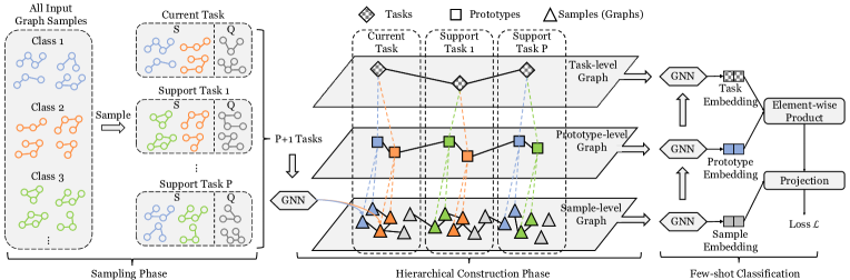
In this section, we introduce the overall structure of our proposed framework FAITH in detail. As illustrated in Figure 1, to capture task correlations among meta-training tasks and thus facilitate the meta-knowledge transfer and adaptation, we build a three-layer hierarchical task graph for each meta-training task in a bottom-up manner. Specifically, for each current meta-training task, we sample additional tasks, denoted as support tasks, via a loss-based sampling strategy. Then these tasks (including the current task) form the hierarchical task graph. Here three layers consist of graph sample nodes, prototype nodes (i.e., the centroid of graph samples of the same class in a task), and task nodes, respectively. In this way, the correlations in graph samples and prototypes from different tasks can be aggregated and propagated among tasks. Then a task-specific classifier utilizes task embeddings learned from the hierarchical task graph for classification on the query set. As a result, the transferred meta-knowledge from other tasks can benefit the classification of each task. Next, we will elaborate on these three key steps.
3.1 Loss-based Sampling for Support Tasks
We aim to sample support tasks to build a hierarchical task graph for each meta-training task; however, random sampling may result in insufficient task correlations caused by huge variance among tasks. Thus, to reduce the task variance, we propose to sample tasks with correlated classes. We assume that the correlated classes for a specific class should consist of graph samples with similar classification results. Therefore, we use a classifier to find correlated classes for a task. Then the classification probability will be used as the sampling probability of each class.
Suppose that we have randomly sampled a meta-training task with a support set consisting of graph samples, where each of classes consists of graph samples. It is noteworthy that these classes are sampled from , where and . To sample tasks that have strong correlations with , we need to sample classes that are correlated with classes in . Therefore, we propose to obtain the sampling probability (i.e., the probability for a class to be sampled) of each class via an MLP layer. Here we use to denote the embedding of the -th graph sample of the -th class with dimension in , learned with . Then the sampling probabilities are generated as:
| (1) |
where is the sampling probability of the -th prototype for all classes. The final sampling probability is computed by averaging: , where is the final sampling probability for all classes. To refine the sampling strategy during training, we calculate the loss for sampling probabilities as follows:
| (2) |
where and if the -th prototype belongs to the -th class of all classes; otherwise . denotes the -th element of . In this way, the sampling loss is incorporated into model training to improve the sampling process. According to , we can sample different classes from all classes to form a new task. In this way, we ensure that classes in the new task are more correlated with classes in , such that the new task could have stronger task correlations with . Similar to , graph samples are randomly sampled for each of classes, which form a new task with graph samples as the support set. Additionally, query graph samples are sampled to form the query set of this task. After repeating this process for times, we obtain support tasks for the hierarchical task graph.
3.2 Constructing Hierarchical Task Graphs
Although we have selected tasks with strong correlations for the hierarchical task graph, it still remains challenging to capture the implicit correlations among these tasks. The reason is that these tasks have different distributions of graph samples and classes. Hence, we propose to build a three-layer hierarchical task graph to capture task correlations. Specifically, the hierarchical graph contains three layers consisting of graph sample nodes, prototype nodes (i.e., the centroid of different classes in each task), and task nodes, respectively. Moreover, the connections between layers are constructed based on the composing relations among tasks, classes, and graph samples. For example, the graph sample nodes are connected to their corresponding prototype node in the next layer. In this way, task correlations can be captured comprehensively with graph samples and classes. To build the graph in each layer, we propose to utilize a novel similarity learning strategy based on both label information and node embeddings to learn an adjacency matrix for this graph. The detailed construction process of these three layers is introduced below.
3.2.1 Sample-level Graph:
Since each task consists of multiple graph samples, task correlations largely exist among graph samples. Hence, we first build a sample-level graph which consists of all graph samples in tasks. In this way, the sample-level graph contains graph samples in total as nodes. In this sample-level graph, graph samples from different tasks are connected to capture sample-level correlations.
Specifically, the input embeddings for nodes in the sample-level graph are denoted as , obtained via the embedding model . denotes the embedding size. To capture the correlations among graph samples, we learn an adjacency matrix to model the connections. In particular, we propose to learn the adjacency matrix based on both node embeddings and label information: , where , and . Here denotes the final adjacency matrix, and and are learned from node embeddings and label information, respectively. Based on the cosine similarity, we obtain , where denotes the -th row vector of . Then is learned based on the labels of samples:
| (3) |
where means the -th and the -th samples are of the same class. In this way, the label information is combined with node embeddings to build connections among graph samples. With , we perform message propagation:
| (4) |
where denotes the output node embeddings of the and is the output dimension size. Then, to build the connections from graph samples to prototypes in the next layer (i.e., the prototype-level graph), we propose to learn weights to aggregate sample embeddings in the same class as the corresponding prototype node embedding. In this way, the input prototype embeddings of the prototype-level graph are obtained from its graph samples that have absorbed the knowledge from other tasks with strong correlations. To generate the aggregation weights, we apply another GNN model:
| (5) |
where denotes the aggregation weights for each sample node, and the output dimension size of is 1. It should be noted that we assume query samples are unlabeled, so the aggregation step is only performed on support samples. Then to produce an input embedding for the -th prototype node in the next layer (i.e., the prototype-level graph), we perform aggregation with its graph samples as follows. We first extract its corresponding entries from and to form and . Then a softmax function is applied to normalize the weights:
| (6) |
where denotes the embedding of the -th prototype (i.e., the -th row vector of of all prototypes) These prototype embeddings will be used as the input node embeddings of the next layer that consists of prototype nodes (since each task has classes).
3.2.2 Prototype-level Graph:
To capture task correlations among prototypes, we propose to build a prototype-level graph that consists of all prototypes in tasks. Since the correlations in the sample-level graph have been aggregated into the prototype embeddings, we can connect these prototype nodes to propagate the information of prototypes from different tasks. In this way, the task correlations can be captured among prototypes via message propagation. Similarly, with tasks, we have prototypes in total. Then a prototype-level graph is built with prototypes as nodes, and the input node embeddings are obtained via the aggregation process of the sample-level graph. To generate the adjacency matrix of this graph, we utilize label information and node embeddings in the same way as the sample-level graph to learn an adjacency matrix: . Similarly to the sample-level graph, and are learned from embeddings and label information of prototypes, respectively. With the learned , we also apply another two GNN models and to perform message propagation and aggregate prototypes nodes, respectively, in the same way as the sample-level graph. Specifically, the output embeddings of this layer are aggregated into their corresponding task nodes to obtain the final input embeddings for the next layer, where is the output dimension size of the prototype-level graph.
3.2.3 Task-level Graph:
Finally, to explicitly characterize task correlations, we build a task-level graph, which consists of tasks as nodes. The task correlations are aggregated into each task node from the previous layer, and messages are propagated among different tasks in this layer. In this way, the task correlations can be captured and facilitate the transfer of meta-knowledge. With the input task embeddings obtained from the previous layer, we first learn an adjacency matrix based on the task node embeddings: , where denotes the -th row vector of . Then the message propagation is performed with another GNN model: where denotes the output task node embeddings. is the output dimension size of the task-level graph.
So far, we have constructed the hierarchical task graph that consists of three layers. In this way, the task correlations are captured at different granularities and facilitate the transfer of meta-knowledge among all tasks.
3.3 Task-specific Few-shot Classification
In this part, the process of task-specific few-shot classification is described in detail. Now from the hierarchical task graph, we have obtained comprehensive embeddings for graph samples, prototypes, and tasks. These embeddings are learned via the correlations among tasks, which can provide more useful knowledge for classification. Therefore, we propose to combine the learned embeddings in each task to conduct task-specific classification for query graph samples. In this way, the unique information of each task can be incorporated into the classification process for better performance.
Specifically, we combine prototype and task embeddings with graph sample embeddings to conduct classification, where all three types of embeddings are learned from the hierarchical task graph. The embeddings matrices are , , and for graph samples, prototypes and tasks, respectively, where and . It is noteworthy that during each training step, query samples in all tasks will be classified for optimization, while during test, only query samples in the target task will be classified. Here we denote and as the embeddings of the -th query sample and the -th prototype in the -th task, respectively. denotes the representation of the -th task. To incorporate information from prototypes and tasks into the classification process, we classify graph samples based on embeddings of their corresponding prototypes and tasks. In particular, we propose to utilize the projected dot product to calculate the classification scores:
| (7) |
where denotes the classification score of the -th graph sample with respect to the -th class in the -th task and is a trainable parameter matrix. denotes the element-wise production. After the normalization , the classification loss is
| (8) |
where denotes whether the -th sample belongs to the -th class in the -th task. represents the corresponding classification score. Combined with the loss produced during the sampling process, the final loss becomes
| (9) |
where is a weight hyper-parameter for . After training, the same process is conducted on target tasks for evaluation. However, the support tasks are also sampled from , since is infeasible. Hence, the only difference between training and evaluation is that the current task is from .
| Methods | Letter-high | ENZYMES | TRIANGLES | Reddit-12K | ||||
|---|---|---|---|---|---|---|---|---|
| 5-shot | 10-shot | 5-shot | 10-shot | 5-shot | 10-shot | 5-shot | 10-shot | |
| WL | ||||||||
| Graphlet | ||||||||
| PN | ||||||||
| Relation | ||||||||
| GSM | ||||||||
| AS-MAML | ||||||||
| FAITH | ||||||||
4 Experiments
In this section, we evaluate FAITH on four widely used graph classification datasets in the few-shot scenario. Then we further demonstrate how different modules of our framework contribute to the classification performance. Codes and data are available at https://github.com/SongW-SW/FAITH.
4.1 Datasets
We follow the work of Chauhan et al. (2020) to evaluate our framework on four processed graph classification datasets, Letter-high, ENZYMES, TRIANGLES and Reddit-12K. Letter-high contains graphs that represent distorted letter drawing, and ENZYMES contains tertiary protein structures. TRIANGLES consists of 10 different classes denoting the number of triangles/3-cliques in each graph, and Reddit-12K contains graphs corresponding to a thread in which nodes represent users and edges represents interactions. The detailed statistics are shown in Table 2.
| Dataset | / | # Graphs | # Nodes | # Edges |
|---|---|---|---|---|
| Letter-high | 4/11 | 2,250 | 4.67 | 4.50 |
| ENZYMES | 2/4 | 600 | 32.63 | 62.14 |
| TRIANGLES | 3/7 | 2,000 | 20.85 | 35.50 |
| Reddit-12K | 4/7 | 1,111 | 391.41 | 456.89 |
4.2 Experimental Settings
To verify the effectiveness of our proposed framework, we compare its performance with different baselines. For graph kernel methods, we compare WL Kernel Shervashidze et al. (2011) and Graphlet Kernel Shervashidze et al. (2009). We also compare Prototypical Network Snell et al. (2017) and Relation Network Sung et al. (2018) which are classic few-shot learning methods. For few-shot graph classification methods, we compare two recent works: GSM Chauhan et al. (2020) and AS-MAML Ma et al. (2020).
All baselines and our proposed framework FAITH are implemented based on PyTorch Paszke et al. (2017). We adopt the classification accuracy as the evaluation metric. We follow the setting of Chauhan et al. (2020) to split the classes in each dataset into training classes and test classes . We specify and , where is the number of labeled graph samples for each class, and is the number of unlabeled graph samples in each task. The number of support tasks during each training step is 10. The dimension of GCN Kipf and Welling (2017) used in the hierarchical task graph is set as . We utilize a 5-layer GIN Xu et al. (2019) with the hidden dimension as the embedding model . For the model optimization, we adopt Adam Kingma and Ba (2015) with a learning rate of 0.001, a dropout rate of 0.5, and the loss weight . The number of training steps and target tasks are set as 1000 and 200, respectively.
4.3 Overall Evaluation Results
We present the performance of few-shot graph classification by different methods in Table 1. Specifically, to demonstrate the classification performance with different sizes of the support set, we show the results with both 5 and 10 support samples for each class (i.e., the number of shots). The results of WL, Graphlet, and GSM are fetched from Chauhan et al. (2020), and other results are obtained by our experiments. From the results, we can observe that our proposed framework FAITH outperforms all other baselines in all datasets with different numbers of support samples, which validates the effectiveness of FAITH on few-shot graph classification. Meanwhile, Prototypical Network Snell et al. (2017) still gains considerable results compared with recent methods AS-MAML Ma et al. (2020) and GSM Chauhan et al. (2020), which demonstrates that combined with GNNs, traditional few-shot learning frameworks can also achieve comparable results. Moreover, the improvements of FAITH over other baselines are slightly higher on ENZYMES. The reason is that in this real-world molecular graph dataset, the task correlations are stronger and thus transfer more beneficial meta-knowledge to each task for classification. Meanwhile, our model can better exploit such correlations among tasks via the hierarchical task graph. In addition, when increasing the number of support samples (i.e., the number of shots) from 5 to 10, the performance of all methods increases differently. Meanwhile, FAITH gains more significant improvements. The reason is that a larger support set in a task can provide stronger task correlations for other tasks.
4.4 Ablation Study
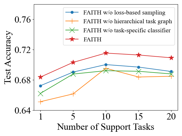
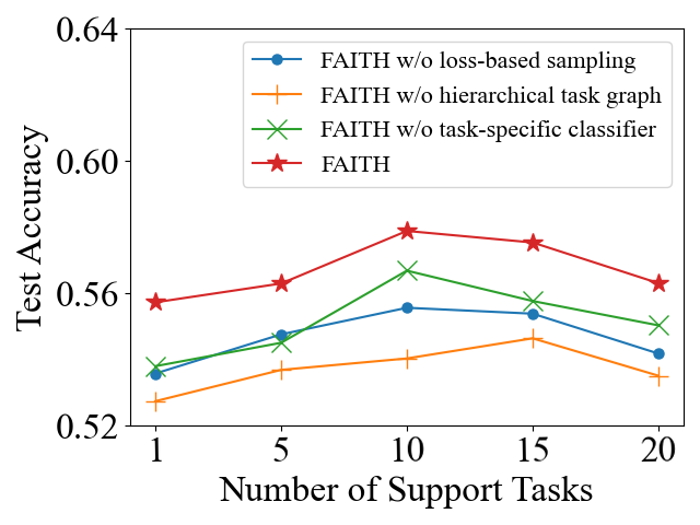
In this part, we validate the importance of three essential modules of FAITH by performing an ablation study with three variants on the 5-shot setting while varying the number of support tasks from 1 to 20. To verify the impact of the loss-based sampling strategy, we replace it with random sampling as the first variant, which ignores the variance in different classes. The second variant removes the hierarchical task graph, and task embeddings are directly computed by averaging all graph sample embeddings in each task. The last variant replaces the task-specific classifier with a Euclidean distance-based classifier, which means the task-specific information is not incorporated into the classification process. The ablation study results of FAITH on Letter-high and ENZYMES datasets are presented in Figure 2. From the results, we observe that all three modules play crucial roles in FAITH. Specifically, the removal of the hierarchical task graph causes a great decrease in the few-shot graph classification performance. Moreover, the loss-based sampling strategy brings a decent performance increase. More importantly, without the task-specific classifier, the performance improvement brought by increasing the number of support tasks becomes less impressive, demonstrating the significance of this module in transferring meta-knowledge among tasks.
4.5 Effects of and
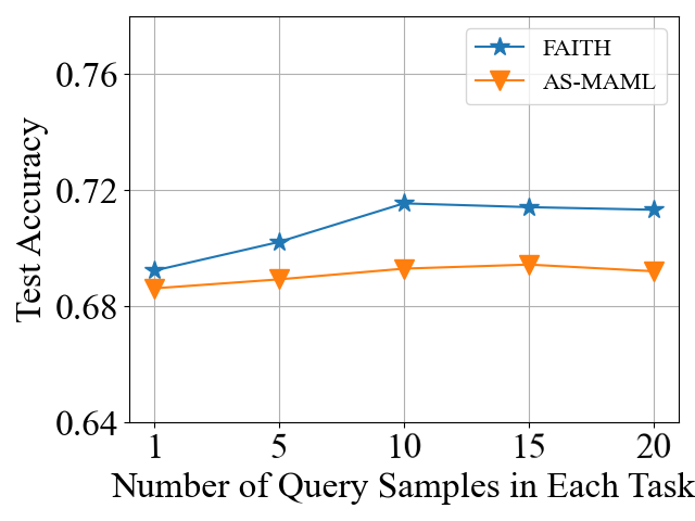
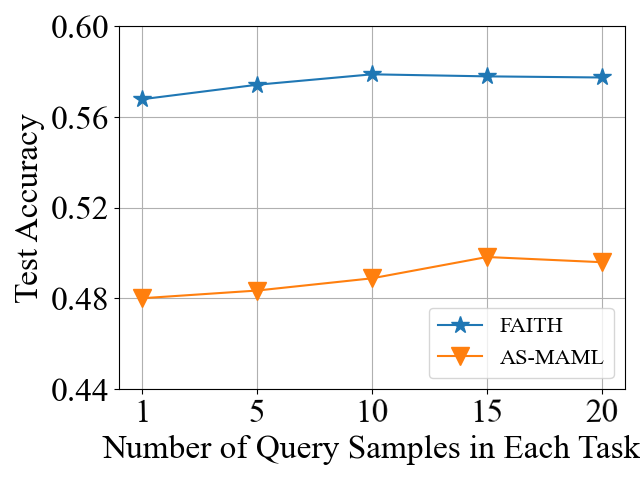
In this subsection, we conduct experiments to show how the number of query instances in each meta-training task and the number of support tasks in a hierarchical task graph affect the performance of our proposed model FAITH. Figure 2 (the curve of FAITH) and Figure 3 report the results of FAITH when varying and on the datasets Letter-high and ENZYMES. Specifically, is set to 10 when we vary the value of , and similarly, is set to 10 when the value of is changed. From Figure 2 and 3, we can observe that involving more query samples during training (i.e., increasing the value of ) slightly increases the performance as a larger number of training samples helps alleviate the over-fitting problem. Moreover, the few-shot graph classification results of FAITH first increase as increases. The reason is that a hierarchical task graph consisting of more support tasks can construct more complex task correlations and thus benefit the transfer of meta-knowledge. However, as the number of support tasks further increases, the performance drops slightly due to the redundancy of irrelevant meta-knowledge transferred from other tasks to the target task. During test, there will be more graph samples from meta-training tasks, which may propagate redundant knowledge to the current test task. Nevertheless, our proposed model FAITH consistently outperforms the state-of-the-art model AS-MAML, which also demonstrates the effectiveness of FAITH.
5 Related Work
5.1 Graph Classification
The task of graph classification aims at assigning a class label from a given label set to each unlabeled graph. Existing methods for graph classification can be broadly divided into two categories. The first category measures the similarity between graphs based on graph kernels for classification. Classic graph kernels include Graphlet Shervashidze et al. (2009) and Weisfeiler-Lehman Shervashidze et al. (2011). The second category utilizes Graph Neural Networks (GNNs) Kipf and Welling (2017); Xu et al. (2019); Veličković et al. (2018); Bai et al. (2019); Xu et al. (2018) to learn discriminative embeddings for nodes via recursively passing the message from their neighbor nodes with a specific aggregation mechanism. Then the node embeddings are aggregated to obtain a global embedding for the graph. For example, SAGPool Lee et al. (2019) proposes a self-attention pooling mechanism that considers both node features and graph topology. Graph U-net Gao and Ji (2019) designs an encoder-decoder model based on two inverse operations of pooling and unpooling.
5.2 Few-shot Learning
Few-shot learning aims at learning a good classification model for the classes that come with a limited amount of training samples Ding et al. (2020); Zhang et al. (2019); Wang et al. (2021); Tan et al. (2022); Xiong et al. (2018). Generally, there are two categories for few-shot learning: metric-based models and optimization-based models. The former type aims at learning an effective distance metric with a well-designed matching function to measure the distance between classes. Then the samples in the query set can be classified according to their distances to samples in the support set. One classic example is Matching Networks Vinyals et al. (2016), which output predictions for query samples via the similarity between query sample and each support sample. The latter type of method optimizes the model parameters via gradient descent on few-shot samples such that the model can be quickly generalized to new classes. For instance, MAML Finn et al. (2017) updates parameters with several gradient descent steps in each task for fast adaptations to new data, while LSTM-based meta-learner Ravi and Larochelle (2016) learns different step sizes for more effective model optimization.
6 Conclusion
In this paper, we study the problem of few-shot graph classification caused by insufficient labeled graphs. We propose a novel few-shot framework FAITH that builds a hierarchical task graph to capture task correlations among meta-training tasks and facilitates the transfer of meta-knowledge to the target task. To address the associated challenges resulting from constructing the task graph, we propose to utilize a loss-based sampling strategy to sample tasks with stronger correlations for the task graph. We further leverage learned task embeddings to incorporate task-specific information into the classification process. Extensive experimental results on four widely used graph datasets demonstrate the superiority of FAITH over other state-of-the-art baselines on few-shot graph classification. Moreover, the ablation study also verifies the effectiveness of each module in FAITH.
7 Acknowledgments
Song Wang, Yushun Dong, and Jundong Li are partially supported by the National Science Foundation (NSF) under grant #2006844.
References
- Bai et al. [2019] Yunsheng Bai, Hao Ding, Song Bian, Ting Chen, Yizhou Sun, and Wei Wang. Simgnn: A neural network approach to fast graph similarity computation. In WSDM, 2019.
- Chauhan et al. [2020] Jatin Chauhan, Deepak Nathani, and Manohar Kaul. Few-shot learning on graphs via super-classes based on graph spectral measures. In ICLR, 2020.
- Ding et al. [2020] Kaize Ding, Jianling Wang, Jundong Li, Kai Shu, Chenghao Liu, and Huan Liu. Graph prototypical networks for few-shot learning on attributed networks. In CIKM, 2020.
- Finn et al. [2017] Chelsea Finn, Pieter Abbeel, and Sergey Levine. Model-agnostic meta-learning for fast adaptation of deep networks. In ICML, 2017.
- Gao and Ji [2019] Hongyang Gao and Shuiwang Ji. Graph u-nets. In ICML, 2019.
- Guo et al. [2021] Zhichun Guo, Chuxu Zhang, Wenhao Yu, John Herr, Olaf Wiest, Meng Jiang, and Nitesh V Chawla. Few-shot graph learning for molecular property prediction. In WWW, 2021.
- Huang and Zitnik [2020] Kexin Huang and Marinka Zitnik. Graph meta learning via local subgraphs. In NeurIPS, 2020.
- Kingma and Ba [2015] Diederik P Kingma and Jimmy Ba. Adam: A method for stochastic optimization. In ICLR, 2015.
- Kipf and Welling [2017] Thomas N Kipf and Max Welling. Semi-supervised classification with graph convolutional networks. In ICLR, 2017.
- Lee et al. [2019] Junhyun Lee, Inyeop Lee, and Jaewoo Kang. Self-attention graph pooling. In ICML, 2019.
- Li et al. [2019] Huaiyu Li, Weiming Dong, Xing Mei, Chongyang Ma, Feiyue Huang, and Bao-Gang Hu. Lgm-net: Learning to generate matching networks for few-shot learning. In ICML, 2019.
- Lichtenstein et al. [2020] Moshe Lichtenstein, Prasanna Sattigeri, Rogerio Feris, Raja Giryes, and Leonid Karlinsky. Tafssl: Task-adaptive feature sub-space learning for few-shot classification. In ECCV, 2020.
- Ma et al. [2020] Ning Ma, Jiajun Bu, Jieyu Yang, Zhen Zhang, Chengwei Yao, Zhi Yu, Sheng Zhou, and Xifeng Yan. Adaptive-step graph meta-learner for few-shot graph classification. In CIKM, 2020.
- Paszke et al. [2017] Adam Paszke, Sam Gross, Soumith Chintala, Gregory Chanan, Edward Yang, Zachary DeVito, Zeming Lin, Alban Desmaison, Luca Antiga, and Adam Lerer. Automatic differentiation in pytorch. In NeurIPS, 2017.
- Ravi and Larochelle [2016] Sachin Ravi and Hugo Larochelle. Optimization as a model for few-shot learning. In ICLR, 2016.
- Shervashidze et al. [2009] Nino Shervashidze, SVN Vishwanathan, Tobias Petri, Kurt Mehlhorn, and Karsten Borgwardt. Efficient graphlet kernels for large graph comparison. In AISTATS, 2009.
- Shervashidze et al. [2011] Nino Shervashidze, Pascal Schweitzer, Erik Jan Van Leeuwen, Kurt Mehlhorn, and Karsten M Borgwardt. Weisfeiler-lehman graph kernels. Journal of Machine Learning Research, 2011.
- Snell et al. [2017] Jake Snell, Kevin Swersky, and Richard Zemel. Prototypical networks for few-shot learning. In NeurIPS, 2017.
- Sung et al. [2018] Flood Sung, Yongxin Yang, Li Zhang, Tao Xiang, Philip HS Torr, and Timothy M Hospedales. Learning to compare: relation network for few-shot learning. In CVPR, 2018.
- Suo et al. [2020] Qiuling Suo, Jingyuan Chou, Weida Zhong, and Aidong Zhang. Tadanet: Task-adaptive network for graph-enriched meta-learning. In SIGKDD, 2020.
- Tan et al. [2022] Zhen Tan, Kaize Ding, Ruocheng Guo, and Huan Liu. Graph few-shot class-incremental learning. In WSDM, 2022.
- Veličković et al. [2018] Petar Veličković, Guillem Cucurull, Arantxa Casanova, Adriana Romero, Pietro Liò, and Yoshua Bengio. Graph attention networks. In ICLR, 2018.
- Vinyals et al. [2016] Oriol Vinyals, Charles Blundell, Timothy Lillicrap, Daan Wierstra, et al. Matching networks for one shot learning. In NeurIPS, 2016.
- Wang et al. [2021] Song Wang, Xiao Huang, Chen Chen, Liang Wu, and Jundong Li. Reform: Error-aware few-shot knowledge graph completion. In CIKM, 2021.
- Xiong et al. [2018] Wenhan Xiong, Mo Yu, Shiyu Chang, Xiaoxiao Guo, and William Yang Wang. One-shot relational learning for knowledge graphs. In EMNLP, 2018.
- Xu et al. [2018] Keyulu Xu, Chengtao Li, Yonglong Tian, Tomohiro Sonobe, Ken-ichi Kawarabayashi, and Stefanie Jegelka. Representation learning on graphs with jumping knowledge networks. In ICML, 2018.
- Xu et al. [2019] Keyulu Xu, Weihua Hu, Jure Leskovec, and Stefanie Jegelka. How powerful are graph neural networks? In ICLR, 2019.
- Yao et al. [2020] Huaxiu Yao, Chuxu Zhang, Ying Wei, Meng Jiang, Suhang Wang, Junzhou Huang, Nitesh Chawla, and Zhenhui Li. Graph few-shot learning via knowledge transfer. In AAAI, 2020.
- Zhang et al. [2019] Chuxu Zhang, Huaxiu Yao, Chao Huang, Meng Jiang, Zhenhui Li, and Nitesh V Chawla. Few-shot knowledge graph completion. In AAAI, 2019.
- Zhou et al. [2019] Fan Zhou, Chengtai Cao, Kunpeng Zhang, Goce Trajcevski, Ting Zhong, and Ji Geng. Meta-gnn: On few-shot node classification in graph meta-learning. In CIKM, 2019.