Variance-Gamma (VG) model: Fractional Fourier Transform (FRFT)

Abstract

The paper examines the Fractional Fourier Transform (FRFT) based technique as a tool for obtaining the probability density function and its derivatives, and mainly for fitting stochastic model with the fundamental probabilistic relationships of infinite divisibility. The probability density functions are computed, and the distributional proprieties are reviewed for Variance-Gamma (VG) model. The VG model has been increasingly used as an alternative to the Classical Lognormal Model (CLM) in modelling asset prices. The VG model was estimated by the FRFT. The data comes from the SPY ETF historical data. The Kolmogorov-Smirnov (KS) goodness-of-fit shows that the VG model fits the cumulative distribution of the sample data better than the CLM. The best VG model comes from the FRFT estimation.

1 Introduction

Several empirical studies have shown that asset returns are often characterized by leptokurtosis and asymmetry. These facts provide evidence suggesting the assumptions of the Classical Lognormal Model (CLM) are not consistent with the empirical observations. A natural generalization of the CLM is the method of subordination[1, 2], which has been used to reduce the theoretical-empirical gap. The subordinated process is obtained by substituting the physical time in the CLM by any independent and stationary increments random process, called the subordinator. If we consider the random process to be a Gamma process, we have a Variance Gamma (VG) model, which is the model the paper will be investigating. The Variance Gamma (VG) model was proposed by Madan[3]. In contrast to the CLM, the VG model does not have an explicit closed-form of the probability density function and its derivatives. In the paper, the VG model has five parameters: parameters of location ($\mu$), symmetric ($\delta$), volatility ($\sigma$), and the Gamma parameters of shape ($\alpha$) and scale ($\theta$). The VG model density function is proven to be (1).

$$f(y)=\frac{1}{\sigma\Gamma(\alpha)\theta^{\alpha}}\int_{0}^{+\infty}\frac{1}{\sqrt{2\pi v}}e^{-\frac{(y-\mu-\delta v)^{2}}{2v\sigma^{2}}}v^{\alpha-1}e^{-\frac{v}{\theta}}\,dv$$ (1)

The integral (1) makes it difficult to utilize the density function and its derivatives, and to perform the Maximum likelihood method. However, in the literature, many studies have found a way to circumvent the lack of closed form by decreasing the number of parameters and using approximation function or analytical expression with modified Bessel function. In fact, [4] developed a procedure to approximate  (1) by Chebyshev Polynomials expansion. [5] and [6] got (1) by analytical expression with modified Bessel function of second kind and third kind respectively. [7] got (1) through Gauss-Laguerre quadrature approximation with Laguerre polynomial of degree $10$.[2] used the Fast Fourier Transform (FFT).
The Fractional Fourier Transform (FRFT) will be implemented on the Fourier Transform of the VG model function (1) and its derivatives. The paper is structured as follows; the next section presents the analytical framework. The third section presents the Variance Gamma (VG) model and the sample data before performing the parameter estimations of the VG model and the Kolmogorov-Smirnov (KS) goodness-of-fit test.

2 Analytical Framework

2.1 Fast Fourier Transform (FFT)

The continuous Fourier transform (CFT) of function $f(t)$ and its inverse are defined by:

$$F[f](x)=\int_{-\infty}^{+\infty}\!f(y)e^{-ixy}\,\mathrm{d}y\quad f(x)=\frac{1}{2\pi}\int_{-\infty}^{+\infty}\!F[f](y)e^{ixy}\,\mathrm{d}y$$ (2)

where i is the imaginary unit.
The Fast Fourier Transform (FFT) is commonly used to evaluate the integrals (2) . The fundamentally inflexible nature [8] of FFT is the main weakness of the algorithm. The advantages of computing with the FRFT [8] can be found at three levels: (1) both the input function values $f(x_{k})$ and the output transform values $F[f](x_{k})$ are equally spaced; (2) a large fraction of $f(x_{k})$ are either zero or smaller than the computer machine epsilon; and (3) only a limited range of $f(x_{k})$ are required.
The FRFT is set up on $n$-long sequence ($x_{1}$, $x_{2}$, …, $x_{n}$) and the Discrete Fourier Transform (DFT), $G_{k}(x,\delta)$, can be shown in [9] to be a composition of ${DFT}^{-1}$ and ${DFT}$.

$$G_{k}(x,\delta)=\sum_{j=0}^{n-1}\!x_{i}e^{-2\pi ijk\delta}\hskip 14.22636pt\hbox{$0\leq k<M$}\quad G_{k}(x,\delta)=e^{-\pi ik^{2}\delta}{DFT}_{k}^{-1}[{{DFT}_{j}(y){DFT}_{j}(z)}]$$ (3)

where ${DFT}^{-1}$ is the inverse of the Discrete Fourier Transform (DFT). We assume that $F[f](t)$ is zero outside the interval $[-\frac{a}{2},\frac{a}{2}]$, and $\beta=\frac{a}{n}$ is the step size of the $n$ input values $F[f](t)$; we define $t_{j}=(j-\frac{n}{2})\beta$ for $0\leq j<n$. We have also $\gamma$ as the step size of the $n$ output values of $f(t)$ and $x_{k}=(k-\frac{n}{2})\gamma$ for $0\leq k<n$. By choosing the step size $\beta$ on the input side and the step size $\gamma$ in the output side, we fix the FRFT parameter $\delta=\frac{\beta\gamma}{2\pi}$.
The density function $f$ at $x_{k}$ can be written as (4). The proof is provided in [10].

$$\hat{f}(x_{k})=\frac{\gamma}{2\pi}e^{-\pi i(k-\frac{n}{2})n\delta}G_{k}(F[f](y_{j})e^{-\pi ijn\delta}),-\delta)$$ (4)

In order to perform $f(t)$ function from the Fourier Transform (FT), we assume $a=20$, $n=2048$, $\beta=\gamma=\frac{a}{n}$. For more detail on FRFT, see [9].

2.2 Variance Gamma (VG) Distribution

$$X=\mu+\delta V+\sigma\sqrt{V}Z\quad Z\sim N(0,1)\quad V\sim\Gamma(\alpha,\theta)$$ (5)

The Variance Gamma distribution is infinitely divisible. The Fourier transform function has an explicit closed-form in (6).

$$F[f](x)=\frac{e^{-i\mu x}}{\left(1+\frac{1}{2}\theta\sigma^{2}x^{2}+i\delta\theta x\right)^{\alpha}}\quad f(y)=\frac{1}{\sigma\Gamma(\alpha)\theta^{\alpha}}\int_{0}^{+\infty}\frac{1}{\sqrt{2\pi v}}e^{-\frac{(y-\mu-\delta v)^{2}}{2v\sigma^{2}}}v^{\alpha-1}e^{-\frac{v}{\theta}}\,dv$$ (6)

When $\delta=0$, we have Symmetric Variance Gamma (SVG) Model. It can be shown by Cumulant-generating function[11] that

$$E(X)=\mu\quad Var(X)=\alpha\theta\sigma^{2}\quad Skew(X)=0\quad Kurt(X)=3(1+\frac{1}{\alpha})$$ (7)

Fig 3, Fig 3 and Fig 3 display the FRFT estimations of the probability density function with Parameter values: $\mu=-2$, $\delta=0$, $\sigma=1$, $\alpha=1$, $\theta=1$. As shown in Fig 3, the probability density is left asymmetric and right asymmetric when the parameter ($\delta$) is negative and positive respectively. For $\delta=0$, the density function is symmetric, as shown in $(\ref{eq:l6})$. The shape parameter ($\alpha$) impacts the peakedness and tails of the distribution, as illustrated in Fig 3 and $(\ref{eq:l6})$; heavier is the tails, shorter is the peakedness. $\theta$ and $\sigma$ have the same impact on the distribution. As shown in $(\ref{eq:l6})$, both change only the variance.

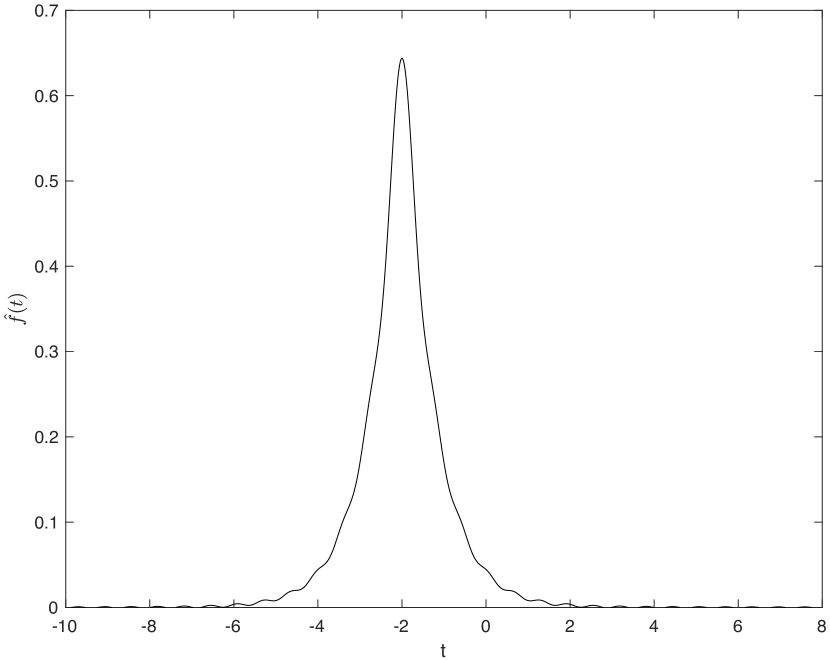
Figure 1: $\hat{f}$: $\mu=-2$,
$\delta=0$, $\sigma=1$, $\alpha=1$, $\theta=1$

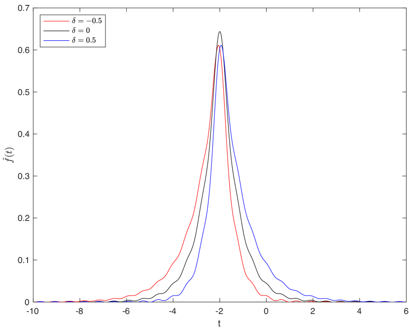
Figure 2: $\hat{f}(t)$
and symmetric parameter($\delta$)

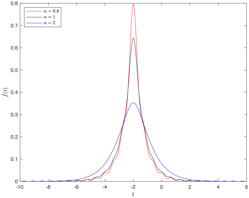
Figure 3: $\hat{f}(t)$
and shape parameter($\alpha$)

3 Variance Gamma (VG) Model

3.1 Model for asset Price

The VG model was introduced by Madan [3]. The asset price is modeled on business time $(k)$ as follows. $\mu,\delta\in R$, $\sigma>0$, $\alpha>0$ and $\theta>0$

$$Y_{k}=\mu+\delta V_{k}+\sigma\sqrt{V_{k}}Z\quad\quad Z\sim N(0,1)\quad V_{k}\sim\Gamma(\alpha,\theta)$$ (8)

$$S_{K}=S_{k-1}e^{\sum_{j=k}^{K}Y_{j}}\quad\quad T_{K}=\sum_{k=1}^{K}V_{k}$$ (9)

$\{T_{k}\}$ is the activity time process, a non-negative stationary independent increment, called the subordinator. $\mu$ is the drift of the physical time scale $t$, $\delta$ is the drift of the activity time process, and $\sigma$ is the volatility. The density of $Y_{j}$ and its Fourier transform were provided in (6). See [10], Appendix A.1, for proof of (6).
$Y_{k}$ is the return variable of the stock or index price, we have (10) from (8) and (9).

$$Y_{k}=log(\frac{S_{k}}{S_{k-1}})\quad\quad E(Y_{k}|V_{k})\sim N(\mu+\delta V_{k},\sigma\sqrt{V_{k}})\quad\quad V_{k}\sim\Gamma(\alpha,\theta)$$ (10)

For $\alpha=\frac{1}{\theta}$  and $0<\theta<<1$, $Y_{k}$ in (8) becomes (11).

$$Y_{k}=\mu+\sigma Z\quad\quad Z\sim N(0,1)$$ (11)

The Classical Lognormal Model (CLM) in (11) is a special case of the Variance - Gamma Model. See [10], Appendix A.1, for proof of (11).

3.2 SPY ETF data

The data comes from the SPY ETF, called SPDR S&P 500 ETF (SPY). The SPY is an Exchange-Traded Fund (ETF) managed by State Street Global Advisors that tracks the Standard & Poor’s 500 index (S&P 500 ), which comprises 500 large and mid-cap US stocks. The SPY ETF is a well-diversified basket of assets listed on the New York Stock Exchange (NYSE). Like other ETFs, SPY ETF provides the diversification of a mutual fund and the flexibility of a stock.
The SPY ETF data was extracted from Yahoo finance. The daily data was adjusted for splits and dividends. The period spans from January 4, 2010, to December 30, 2020. 2768 daily SPY ETF prices were collected, around 252 observations per year, over 10 years. The dynamic of daily adjusted SPY ETF price is provided in Fig 5.
Let the number of observations $N=2768$, and the daily observed SPY ETF price $S_{j}$ on day $t_{j}$ with $j=1,\dots,N$; $t_{1}$ is the first observation date (January 4, 2010) and $t_{N}$ is the last observation date (December 30, 2020). The daily SPY ETF log return $(y_{j})$ is computed as in (12).

$$y_{j}=\log(S_{j}/S_{j-1})\hskip 28.45274pt \hbox{ $j=2,\dots,N$}\\ \vspace{0.2cm}$$ (12)

The results of the daily SPY ETF return  are shown in Fig 5.

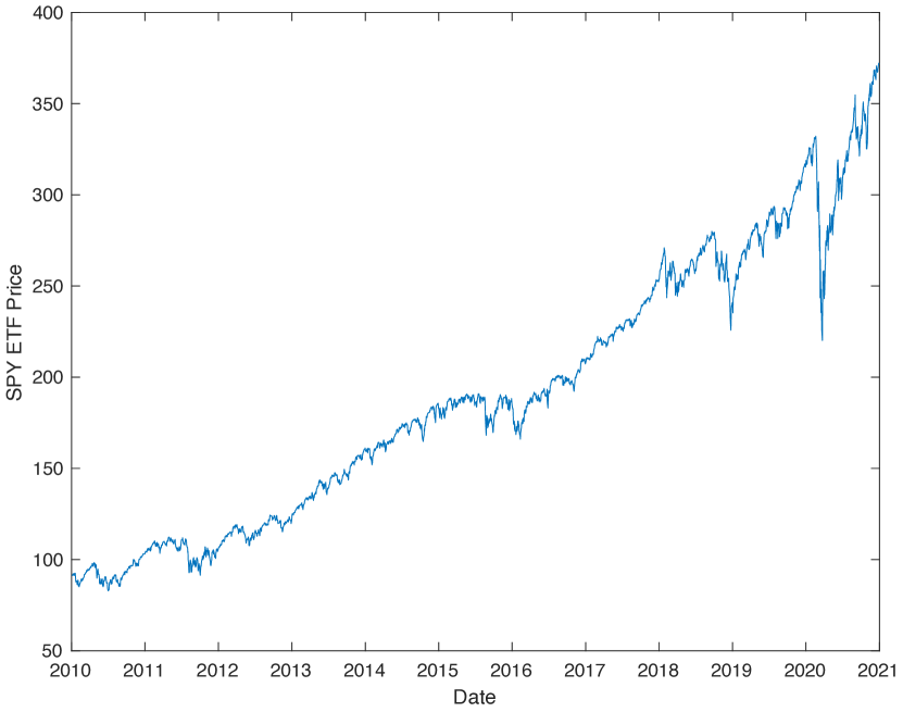
Figure 4: Daily SPY ETF Price

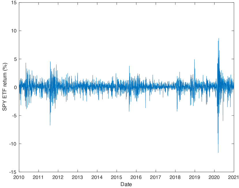
Figure 5: Daily SPY ETF return

As shown in Fig 5 and Fig 5, like other stocks and securities, SPY ETF was unusually volatile in the first quarter of $2020$ amid the coronavirus pandemic and massive disruptions in the global economy. $13$ daily return observations were identified as outliers and removed from the data set in order to avoid a negative impact on the statistics and estimators.

4 Variance Gamma (VG) Model Estimations

From a probability density function $f(y,V)$ with parameter $V$ of size ($p=5$) and the sample data $Y$ of size ($M=2755$), we define the Likelihood function and its derivatives.

$$l(y,V)=\sum_{j=1}^{M}log(f(y_{j},V))\vspace{-0.3cm}$$ (13)

$$\frac{dl(y,V)}{dV_{j}}=\sum_{i=1}^{M}\frac{\frac{df(y_{i},V)}{dV_{j}}}{f(y_{i},V)}$$ (14)

$$\frac{d^{2}l(y,V)}{dV_{k}dV_{j}}=\sum_{i=1}^{M}\left(\frac{\frac{d^{2}f(y_{i},V)}{dV_{k}dV_{j}}}{f(y_{i},V)}-\frac{\frac{df(y_{i},V)}{dV_{k}}}{f(y_{i},V)}\frac{\frac{df(y_{i},V)}{dV_{j}}}{f(y_{i},V)}\right)$$ (15)

With $1\leq k\leq p\ \ and\ \ 1\leq j\leq p$.
$f(y_{i},V)$, $\frac{df(y_{i},V)}{dV_{j}}$, $\frac{d^{2}f(y_{i},V)}{dV_{k}dV_{j}}$ are computed with the FRFT on each $y_{i}$ with $1\leq i\leq M$. See Fig $4$, Fig $5$, Appendix B.2 and Appendix C.3 in [10], these figures display the shape of the quantities $\frac{df(y_{i},V)}{dV_{j}}$, $\frac{d^{2}f(y_{i},V)}{dV_{k}dV_{j}}$, which can be Odd or Even functions.
The Newton Raphson Iteration process in (16) was implemented on the score function ($I^{\prime}(y,V)$), and the Fisher information matrix ($I^{\prime\prime}(y,V)$).

$$V^{n+1}=V^{n}+{\left(I^{\prime\prime}(y,V^{n})\right)^{-1}}I^{\prime}(y,V^{n})$$ (16)

With initial value $\sigma=\alpha=\theta=1$, $\delta=\mu=0$, the maximization procedure convergences after 21 iterations for Asymmetric Variance-Gamma Model (AVG). The result of the iteration Process (16) are shown in Table 1.

Table 1: Results of AVG Model Parameters Estimations

Iterations	$\mu$	$\delta$	$\sigma$	$\alpha$	$\theta$	$l(y,V)$	$||\frac{dl(y,V)}{dV}||$
1	0	0	1	1	1	-3582.8388	598.743231
2	0.05905599	-0.0009445	1.03195903	0.9130208	1.03208412	-3561.5099	833.530396
3	0.06949925	0.00400035	1.04101444	0.88478895	1.05131996	-3559.5656	447.807305
4	0.07514039	0.00055771	1.17577397	0.67326429	1.17778666	-3569.6221	211.365781
5	0.08928373	-0.0263716	1.03756321	0.83842661	0.94304967	-3554.4434	498.289445
6	0.08676498	-0.0521887	1.03337015	0.85591875	0.95066351	-3550.6419	204.467192
7	0.086995	-0.0608517	1.02788937	0.87382621	0.95054954	-3549.8465	66.8039738
8	0.08542912	-0.058547	1.02705241	0.88258411	0.94321299	-3549.7023	15.3209117
9	0.08478622	-0.0576654	1.02995166	0.88447791	0.93670036	-3549.6921	1.14764198
10	0.08477798	-0.0577736	1.02922308	0.88449072	0.93831041	-3549.692	0.17287708
11	0.08476475	-0.0577271	1.02960343	0.88450434	0.93755549	-3549.692	0.07850459
12	0.08477094	-0.0577488	1.02942608	0.8844984	0.93790784	-3549.692	0.03723941
13	0.08476804	-0.0577386	1.02950937	0.88450117	0.93774266	-3549.692	0.01732146
14	0.0847694	-0.0577434	1.02947043	0.88449987	0.93781995	-3549.692	0.00813465
15	0.08476876	-0.0577411	1.02948868	0.88450048	0.93778375	-3549.692	0.00380345
16	0.08476906	-0.0577422	1.02948014	0.88450019	0.9378007	-3549.692	0.00178206
17	0.08476892	-0.0577417	1.02948414	0.88450033	0.93779276	-3549.692	0.00083415
18	0.08476898	-0.0577419	1.02948226	0.88450026	0.93779648	-3549.692	0.00039063
19	0.08476895	-0.0577418	1.02948314	0.88450029	0.93779474	-3549.692	0.00018289
20	0.08476897	-0.0577419	1.02948273	0.88450028	0.93779555	-3549.692	8.56E-05
21	0.08476896	-0.0577418	1.02948292	0.88450029	0.93779517	-3549.692	4.01E-05

The estimation of other models are summarized in Table 2. The method of moments provides the initial values for AVG1 and SVG1 maximization procedure. The results are labeled AVG1 for Asymmetric VG Model and SVG1 for Symmetric VG Model. Another initial value was chosen: $\sigma=\alpha=\theta=1$, $\delta=\mu=0$. The results are labeled AVG2 and SVG2 respectively for Asymmetric VG and Symmetric VG Models.
The Maximum Likelihood estimations are summarized in Table 2.

Table 2: Variance-Gamma Parameters Estimations

Model	$\mu$	$\delta$	$\sigma$	$\alpha$	$\theta$
AVG1	$0.1683$	$-0.1089$	$0.8987$	$0.9284$	$1.0546$
SVG1	$0.0510$		$0.9378$	$0.8490$	$1.0929$
AVG2	$0.0848$	$-0.0577$	$1.0295$	$0.8845$	$0.9378$
SVG2	$0.0652$		$0.9939$	$0.8770$	$0.9937$
CLM	$0.0541$		$0.9740$

The estimation of parameters ($\mu$, $\sigma$) of the Classical Lognormal Model (CLM) was added to Table 2.

5 Comparison of Variance Gamma (VG) Models

which VG model estimation fits the empirical distribution was also considered. The Kolmogorov-Smirnov (KS) test was performed under the null hypothesis (H0) that the sample $\{y_{1},y_{2}\dots y_{n}\}$ comes from VG model. The Kolmogorov-Smirnov (K-S) estimator ($D_{n}$) is defined in (17).

$$\vspace{-0.3cm}D_{n}=\sup_{x}{|F(x)-F_{n}(x)|}\quad P_{value}=prob(D_{n}>d_{n}|H_{0})$$ (17)

$F_{n}(x)$ denotes the empirical cumulative distribution and $n$ is the sample size. The VG cumulative distribution function ($F$) was computed with FRFT from its Fourier.
The cumulative distribution of $D_{n}$[12] under the null hypothesis was computed and the density function was deduced. The computed density function is shown in Fig 6. Under the null hypothesis (H0), $D_{n}$ has a positively skewed distribution with means ($\mu=0.0165$) and standard deviation  ($\sigma=5*10^{-3}$).

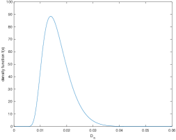
Figure 6: Kolmogorov-Smirnov Estimator ($\hat{D_{n}}$) probability density ($n=2755$)  under the null hypothesis $H{0}$

$d_{n}$ is the value of the KS estimator ($D_{n}$) computed from the sample $\{y_{1},y_{2}\dots y_{n}\}$. Based on [13, 14], $d_{n}$ can be estimated as follows.

$$d^{+}_{n}=\sup_{0\leq j\leq P}{|F(x_{j})-F_{n}(x_{j})|} \quad d^{-}_{n}=\sup_{1\leq j\leq P}{|F(x_{j})-F_{n}(x_{j-1})|}\quad d_{n}=Max(d^{+}_{n},d^{-}_{n})$$ (18)

The statistics estimation for SVG2 model is shown in [10]. $d^{-}_{n}=max((1))=0.023629$, $d^{+}_{n}=max((2))=0.021986$ and $d_{n}=0.023629$. See Appendix E.5, Table E.5 in [10].

For each model, KS-Statistics ($d_{n}$) and P_values were computed, and the results are provided in Table 2.

Table 3: Kolmogorov-Smirnov (KS) test

Model	KS-Statistics ($d_{n}$)	P_values
AVG1	0.054290	0.00001691%
SVG1	0.036763	0.1136%
AVG2	0.028182	2.4668%
SVG2	0.023629	9.0788%
CLM	0.095791	0%

Most KS-statistic $d_{n}$ has high value and suggests that the sample $\{y_{1},y_{2}\dots y_{n}\}$ rejects the null hypothesis (H0), except SVG2 model, and to some extent, AVG2 model at $2\%$ risk level.
As shown in Table 3, VG models from the method of moments do not fit the sample data distribution. The $P\_values$ is less than $5\%$, and the null hypothesis $H_{0}$ can not be accepted at that risk level. The CLM does not fit the sample data distribution at $5\%$. Regarding the maximum likelihood method, the SVG2 model has $P\_values=9.079\%$, which is high than the classical threshold  $5\%$. Therefore, SVG2 model can not be rejected. See [10] for $d_{n}$ and $P\_values$ computations.
The daily SPY ETF return histogram was compared to the density function of two models (SVG2, CLM) as shown in Fig 9 and Fig 9. It results that the peakedness of the histogram explains the high level of the KS-Statistics in Table 3 and the model rejection.

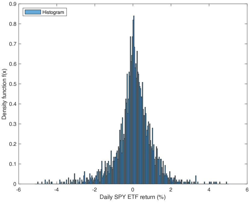
Figure 7: return Histogram

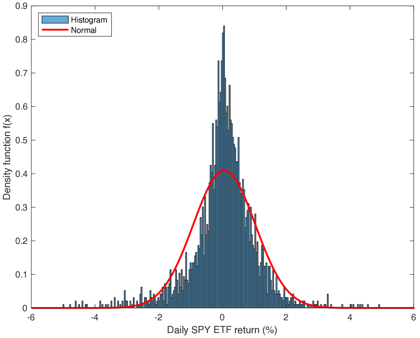
Figure 8: CLM Model

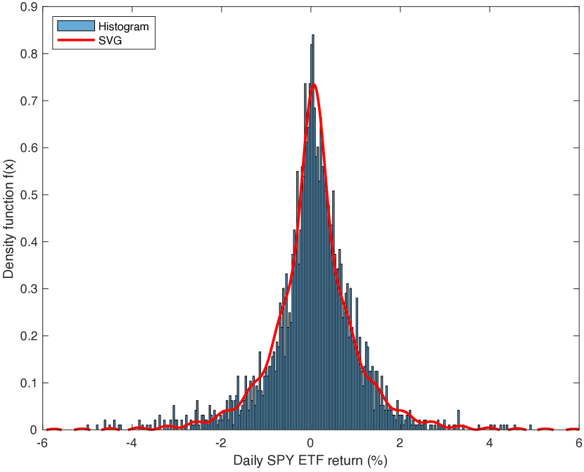
Figure 9: SVG2 Model

For work related to Normal and exponential distributions, see [15, 16, 17, 18]

6 Conclusion

In the study, the FRFT-based technique is used to compute and analyze the probability density function of the Variance-Gamma (VG) model; and perform the estimation of the five parameters of the VG model. The results show that the VG model captures the peakedness and leptokurtosis properties of the daily SPY sample data. The findings provide evidence that the VG model fits better than the CLM Model. The Kolmogorov-Smirnov (KS) goodness-of-fit test shows that the Maximum Likelihood method with FRFT produces a good estimation of the VG model, which fits the empirical distribution of the sample data.

References

References

- [1] Clark P K 1973 Econometrica: journal of the Econometric Society 135–155
- [2] Hurst S R, Platen E and Rachev S T 1997 Financial Engineering and the Japanese Markets 4 97–124
- [3] Madan D B and Seneta E 1990 Journal of business 511–524
- [4] Madan D B and Seneta E 1987 Journal of the Royal Statistical Society: Series B (Methodological) 49 163–169
- [5] Madan D B, Carr P P and Chang E C 1998 Review of Finance 2 79–105
- [6] Seneta E 2004 Journal of Applied Probability 177–187
- [7] Mercuri L and Bellini F 2010 Derivatives eJournal
- [8] Bailey D and Swarztrauber P 1994 SIAM J. Sci. Comput. 15 1105–1110
- [9] Bailey D H and Swarztrauber P N 1991 SIAM review 33 389–404
- [10] Nzokem A H 2021 arXiv preprint arXiv:2104.07580 (Preprint 2104.07580)
- [11] Kendall M G 1945 The advanced theory of statistics. vol 1 (Charles Griffin and Co., Ltd., London)
- [12] Dimitrova D S, Kaishev V K and Tan S 2020 Journal of Statistical Software 95 1–42
- [13] Krysicki W, Bartos J, Dyczka W, Królikowska K and Wasilewski M 1999 Cz. II. Statystyka matematyczna, PWN, Warszawa
- [14] Kucharska M and Pielaszkiewicz J 2009 Halmstad University
- [15] Nzokem A H 2021 International Journal of Statistics and Probability 10 10–20
- [16] Nzokem A H 2020 Stochastic and Renewal Methods Applied to Epidemic Models Ph.D. thesis York University, YorkSpace institutional repository
- [17] Nzokem A and Madras N 2020 Bulletin of Mathematical Biology 82 1–16
- [18] Nzokem A and Madras N 2021 Age-structured epidemic with adaptive vaccination strategy: Scalar-renewal equation approach Recent Developments in Mathematical, Statistical and Computational Sciences (Springer)