Exclusive vector meson productions with the analytical solution of Balitsky-Kovchegov Equation

Abstract

Exclusive vector meson production is an excellent probe for describing the structure of proton. In this paper, based on dipole model, the differential cross sections, total cross sections and the ratios of the longitudinal to transverse cross sections of $J/\psi$ and $\rho^{0}$ productions are calculated with the analytical solution of Balitsky-Kovchegov (BK) equation. In addition, we also consider the influences of two meson wave function models on the results. Our predictions, which are little sensitive to meson wave functions, agree with the experimental data. The analytical solution of BK equation is reliable for description of exclusive vector meson production in a certain range of $Q^{2}$.

I Introduction

Color Glass Condensate (CGC) McLerran and Venugopalan (1994); Iancu et al. (2002); Iancu and Venugopalan (2003); Jalilian-Marian and Kovchegov (2006); Gelis et al. (2010) is an effective theory to describe physics in the proton saturation regime. Inside proton, gluons cannot grow infinitely without breaking the unitary limit. Consequently, in small x regime, recombination and multiple scattering of gluon will reach the balance, then the number of gluons will not increase. This is called gluon saturation, which can be described by CGC effective field theory. For studying proton structure in saturation regime at high energy limit, deep inelastic scattering (DIS), deeply virtual compton scattering (DVCS) and exclusive diffractive vector meson production are excellent probes Gribov et al. (1983); Mueller and Qiu (1986); Mueller (1999).

For analyzing DIS and vector meson production, the color dipole model or CGC effective theory is a powerful tool Nikolaev and Zakharov (1991); Mueller and Patel (1994); Mueller (1994); Kopeliovich and Zakharov (1991); Nikolaev and Zakharov (1991); Kopeliovich et al. (1994); Nemchik et al. (1994, 1996, 1997). In dipole model, virtual photon splits into a quark anti-quark pair (dipole) which interacts with proton by exchanging gluons. Then the dipole recombines into the meson or the photon. Golec-Biernat and Wusthoff (GBW) model Golec-Biernat and Wusthoff (1998) and CGC model Iancu et al. (2004) have a good description of the dipole scattering process. And two impact-parameter dependent models, b-CGC model Watt and Kowalski (2008); Kowalski et al. (2006) which is the modification of CGC model and IP-Sat Kowalski and Teaney (2003); Rezaeian et al. (2013) model are successful in the application of DIS and exclusive vector meson production process Iancu et al. (2004); Lappi and Mantysaari (2011); Kowalski et al. (2008a, b); Xie and Goncalves (2022). Saturation effect in b-CGC model and IP-Sat model is related to Balitsky-Kuraev-Fadin-Lipatov (BFKL) equation Fadin et al. (1975); Kuraev et al. (1976, 1977); Balitsky and Lipatov (1978) and Dokshitzer-Gribov-Lipatov-Altarelli-Parisi (DGLAP) equation Gribov and Lipatov (1972); Dokshitzer (1977); Altarelli and Parisi (1977) respectively Rezaeian and Schmidt (2013). These models are also applied to Large Hadron Collider(LHC) experiment Motyka and Watt (2008); Levin and Rezaeian (2010); Tribedy and Venugopalan (2011, 2011); Xie and Chen (2018).

Besides, the evolution of dipole-target scattering amplitude can be dominated by Balitsky-Kovchegov (BK) equation Balitsky (1997); Kovchegov (1999, 2000); Balitsky (2001) with a nonlinear term for gluon saturation, which is regarded as the mean field approximation of the Jalilian-Marian-Iancu-McLerran-Weigert-Leonidov-Kovner (JIMWLK) equation Balitsky (1996); Jalilian-Marian et al. (1997); Iancu et al. (2001); Weigert (2002). There are a lot of research on the BK equation. The influence of impact parameter b was numerically analyzed for BK equation in Golec-Biernat and Stasto (2003). The solution of the b-dependence BK equation with the collinearly improved kernel has been studied Bendova et al. (2019). Discussion for the behavior of the numerical solution of running coupling BK equation with Runge-Kutta method was presented in Matas et al. (2016). Re. Lappi and Mäntysaari (2015) showed numerical solution to BK equation in the coordinate space at next-to-leading order.

In the momentum space, it has been shown Kovchegov (1999, 2000) that the nonlinear evolution equation with the Balitskii-Fadin-Kuraev-Lipatov (BFKL) kernel is obtained form BK equation by proper approximation. Then, by variable substitution, this nonlinear evolution equation Munier and Peschanski (2003, 2004a, 2004b) is simplified to Fisher-Kolmogorov-Petrovsky-Piscounov (FKPP) equation Fisher (1937) which is a kind of reaction-diffusion nonlinear equation. The analytical solution of BK equation is obtained by solving the more concise FKPP equation. The analytical solution Bondarenko and Prygarin (2015); Marquet et al. (2005); Xiang et al. (2017, 2020, 2021) of BK equation has been studied by different methods. We also obtain the analytical solution of BK equation Wang et al. (2021) in the momentum space. In this work, the analytical solution that we have obtained will be used to explain the scattering process between protons and color dipole.

The arrangement of the article is as follows. In Sec. II, the dipole representation of exclusive vector meson production is reviewed, and overlaps between photon and vector mesons ($J/\Psi$, $\rho^{0}$) wave function are shown. in Sec. III, Our solution of BK equation in momentum space is introduced. And the results of the fitting to the structure function $F_{2}$ of proton with our solution are provided. In Sec. IV, the figures of our calculations for vector mesons ($J/\Psi$, $\rho^{0}$) production differential cross section with $\rm t$ and total cross section as functions of center of mass energy W and the photon virtuality $Q^{2}$ are presented. The ratios of the longitudinal to transverse cross section for $J/\Psi$ and $\rho^{0}$ are shown. Finally, in Sec. V, discussion and summary are given.

II Dipole description of exclusive vector meson production

In the proton rest frame, for exclusive vector meson production in the dipole model representation Rezaeian and Schmidt (2013); Forshaw et al. (2004); Watt and Kowalski (2008), as shown in Fig.  1 (Right), even though the momentum transfer $\bm{\Delta}\neq 0$ ($\rm t=-\bm{\Delta}^{2}$), the imaginary part of its amplitude can be similarly expressed as Kowalski et al. (2006)

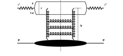
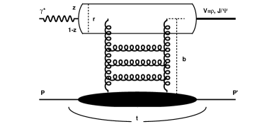
Figure 1: (Left) Elastic scattering amplitude for DIS and (Right) the amplitude of exclusive vector meson production in dipole model.

$$\mathcal{A}_{T,L}^{\gamma^{*}p\rightarrow Vp}(x,Q^{2},t)=\mathrm{i}\int\mathrm{d}^{2}\bm{r}\int_{0}^{1}\frac{\mathrm{d}z}{4\pi}\int\mathrm{d}^{2}\bm{b}$$ (1)

$$\left(\Psi_{V}^{*}\Psi\right)_{T,L}\left(r,z,Q\right)\mathrm{e}^{-\mathrm{i}[\textbf{b}-(1-z)\textbf{r}]\bm{\Delta}}\cdot\frac{\mathrm{~{}d}\sigma_{q\bar{q}}}{\mathrm{~{}d}^{2}\bm{b}}\left(x,r,b\right)$$

$$=\mathrm{i}\int_{0}^{\infty}\mathrm{d}r(2\pi r)\int_{0}^{1}\frac{\mathrm{d}z}{4\pi}\int_{0}^{\infty}\mathrm{d}b(2\pi b)$$

$$\times\left(\Psi_{V}^{*}\Psi\right)_{T,L}J_{0}(b\Delta)J_{0}([1-z]r\Delta)\frac{\mathrm{d}\sigma_{q\bar{q}}}{\mathrm{~{}d}^{2}\bm{b}},$$

where $\left(\Psi_{V}^{*}\Psi\right)_{T,L}$ is the amplitude of the conversion of virtual photon into vector meson. $\frac{\mathrm{~{}d}\sigma_{q\bar{q}}}{\mathrm{~{}d}^{2}\bm{b}}$ is dipole scattering differential cross section where $\bm{b}$ is the impact parameter. Total dipole-target cross section $\sigma_{q\bar{q}}$ will be obtained by the BK equation. And $J_{0}$ is the first kind Bessel function. To get the real part of the amplitude, the ratio of real to imaginary parts of the scattering amplitude will be used.

Thereby, differential cross section for exclusive vector meson production is given by Nemchik et al. (1994, 1997); Forshaw et al. (2004); Kowalski and Teaney (2003); Kowalski et al. (2006)

$$\frac{\mathrm{d}\sigma_{T,L}^{\gamma^{*}p\rightarrow Vp}}{\mathrm{~{}d}t}\left(x,Q^{2},t\right)=\frac{R^{2}_{g}}{16\pi}\left|\mathcal{A}_{T,L}^{\gamma^{*}p\rightarrow Vp}\right|^{2}\left(1+\beta^{2}\right)$$ (2)

where $\beta$ denotes the ratio of real to imaginary parts of the scattering amplitude. $\beta$ is written as

$$\beta=\tan(\pi\lambda/2),\quad\text{ with }\quad\lambda\equiv\frac{\partial\ln\left(\mathcal{A}_{T,L}^{\gamma^{*}p\rightarrow Vp}\right)}{\partial\ln(1/x)}.$$ (3)

And $R^{2}_{g}$ reflects the skewed effect, given by Shuvaev et al. (1999)

$$R_{g}=\frac{2^{2\lambda+3}}{\sqrt{\pi}}\frac{\Gamma(\lambda+5/2)}{\Gamma(\lambda+4)}.$$ (4)

If the dependence of $t$ in the amplitude $\mathcal{A}_{T,L}^{\gamma^{*}p\rightarrow Vp}$ is exponential Ahmady et al. (2016), then Eq.  (2) is rewritten as

$$\frac{\mathrm{d}\sigma_{T,L}^{\gamma^{*}p\rightarrow Vp}}{\mathrm{~{}d}t}\left(x,Q^{2},t\right)=\frac{R^{2}_{g}}{16\pi}\left|\mathcal{A}_{T,L}^{\gamma^{*}p\rightarrow Vp}\right|_{t=0}^{2}\left(1+\beta^{2}\right)e^{-B_{D}|t|}.$$ (5)

Then the total cross section is obtained as

$$\sigma_{T,L}^{\gamma^{*}p\rightarrow Vp}\left(x,Q^{2}\right)=\frac{R^{2}_{g}}{16\pi B_{D}}\left|\mathcal{A}_{T,L}^{\gamma^{*}p\rightarrow Vp}\right|_{t=0}^{2}\left(1+\beta^{2}\right),$$ (6)

$$\sigma_{tot}^{\gamma^{*}p\rightarrow Vp}\left(x,Q^{2}\right)=\sigma_{T}^{\gamma^{*}p\rightarrow Vp}\left(x,Q^{2}\right)+\sigma_{L}^{\gamma^{*}p\rightarrow Vp}\left(x,Q^{2}\right).$$ (7)

where $B_{D}=N\left(14.0\left(\frac{1\mathrm{GeV}^{2}}{Q^{2}+M_{V}^{2}}\right)^{0.2}+1\right)$ with $N=0.55\,\rm GeV^{-2}$ for $\rho^{0}$ Ahmady et al. (2016). For $J/\Psi$, $B_{D}$ is written as Cepila et al. (2019); Chekanov et al. (2002)

$$B_{D}=\begin{cases}4.15+4\times 0.116\ln(\frac{\rm W}{90\,\rm GeV})&Q^{2}\leq 1\rm GeV^{2},\\ 4.72+4\times 0.07\ln(\frac{\rm W}{90\,\rm GeV})&Q^{2}>1\rm GeV^{2},\end{cases}$$ (8)

where $\rm W$ is center of mass energy of $\gamma^{*}p$, which is related to the $x$ and $Q^{2}$ as

$$x\,=\,x_{Bj}(1+M^{2}_{V}/Q^{2})\,=\,\frac{Q^{2}+M^{2}_{V}}{W^{2}+Q^{2}},$$ (9)

where $M_{V}$ is the mass of the vector meson, and $x_{Bj}$ is bjorken scale. For $J/\Psi$, $M_{V}\,=\,3.097\,\rm GeV$, and for $\rho^{0}$, $M_{V}\,=\,0.776\,\rm GeV$.

For overlaps between photon and vector meson wave functions Kowalski et al. (2006), its transverse and longitudinal polarization parts are

$$\left(\Psi_{V}^{*}\Psi\right)_{T}= \hat{e}_{f}e\frac{N_{c}}{\pi z(1-z)}\left\{m_{f}^{2}K_{0}(\epsilon r)\phi_{T}(r,z)\right.$$ (10)

$$\left.-\left[z^{2}+(1-z)^{2}\right]\epsilon K_{1}(\epsilon r)\partial_{r}\phi_{T}(r,z)\right\},$$

$$\left(\Psi_{V}^{*}\Psi\right)_{L}= \hat{e}_{f}e\frac{N_{c}}{\pi}2Qz(1-z)K_{0}(\epsilon r)\left[M_{V}\phi_{L}(r,z)\right.$$

$$\left.+\delta\frac{m_{f}^{2}-\nabla_{r}^{2}}{M_{V}z(1-z)}\phi_{L}(r,z)\right],$$

where $e=\sqrt{4\pi\alpha_{em}}$, $N_{c}=3$, $\nabla_{r}^{2}\equiv(1/r)\partial_{r}+\partial_{r}^{2}$, $\epsilon=\sqrt{z(1-z)Q^{2}+m^{2}_{f}}$, and the effective charge $\hat{e}_{f}$ is $2/3$ or $1/\sqrt{2}$ for $J/\psi$ or $\rho^{0}$. $m_{f}$ is the quark mass. $K_{0}$ and $K_{1}$ are the second kind Bessel function. For scalar wave functions, $\phi_{L}(r,z)$ and $\phi_{T}(r,z)$, there are two models, “Gaus-LC” Kowalski and Teaney (2003) and “boosted Gaussian” Forshaw et al. (2004). It should be noted that we follow the works of other people to use $\delta=0$ for the ”Gaus-LC” model and $\delta=1$ for the ”boosted Gaussian” model as mentioned by H. Kowalski et al Kowalski et al. (2006).

For the “Gaus-LC” model, the scalar wave functions, $\phi_{L}(r,z)$ and $\phi_{T}(r,z)$ are written as

$$\begin{gathered}\phi_{T}(r,z)=N_{T}[z(1-z)]^{2}\exp\left(-r^{2}/2R_{T}^{2}\right),\\ \phi_{L}(r,z)=N_{L}z(1-z)\exp\left(-r^{2}/2R_{L}^{2}\right).\end{gathered}$$ (11)

For the ”boosted Gaussian” model, $\phi_{L}(r,z)$ and $\phi_{T}(r,z)$ are given by

$$\phi_{T}(r,z)= \mathcal{N}_{T}z(1-z)\exp\left(-\frac{m_{f}^{2}\mathcal{R}^{2}}{8z(1-z)}\right.$$ (12)

$$\left.-\frac{2z(1-z)r^{2}}{\mathcal{R}^{2}}+\frac{m_{f}^{2}\mathcal{R}^{2}}{2}\right),$$

$$\phi_{L}(r,z)= \mathcal{N}_{L}z(1-z)\exp\left(-\frac{m_{f}^{2}\mathcal{R}^{2}}{8z(1-z)}\right.$$

$$\left.-\frac{2z(1-z)r^{2}}{\mathcal{R}^{2}}+\frac{m_{f}^{2}\mathcal{R}^{2}}{2}\right).$$

The parameters in the Eq.  (11) and Eq.  (12) can be found in Kowalski et al. (2006). Transversely and longitudinally overlaps between vector meson functions and the photon function integrated over $\rm z$ as a function of dipole size $\rm r$ are presented in Fig. 2.

In the following calculation, both models “Gaus-LC” and “boosted Gaussian” will be used. We will compare the effects of two models on the calculation results.

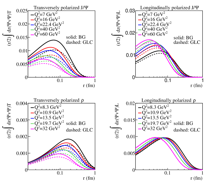
Figure 2: Transversely and longitudinally overlaps between vector meson and the photon functions as a function of dipole size $\rm r$, which are integrated over $\rm z$ is presented. Solid line is for “Boosted Gaussian” (BG) model, and dashed line is for “Gaus-LC” (GLC) model.

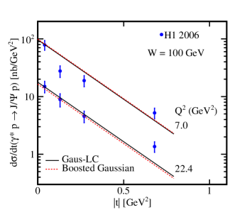
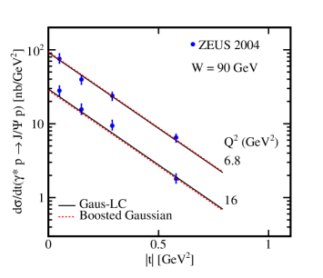
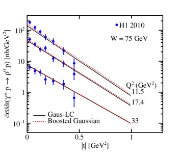
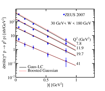
Figure 3: (above) Calculations of differential cross section of $\gamma^{*}p\rightarrow J/\Psi p$ as a function of $|\rm t|$ compared with experimental data from ZEUS 2004 Chekanov et al. (2004) and H1 2005 Aktas et al. (2006) using two different meson wave functions. (Bottom) Prediction of differential cross section of $\gamma^{*}p\rightarrow\rho^{0}p$ as a function of $|\rm t|$ compared with experimental data from ZEUS 2007 and H1 2010 Chekanov et al. (2007); Aaron et al. (2010a).

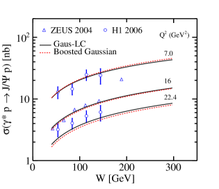
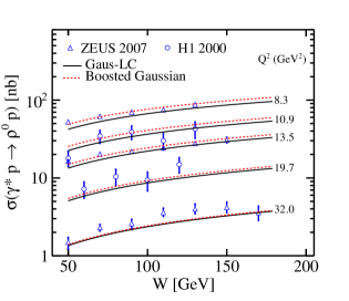
Figure 4: (Left) Prediction of total cross sections of $\gamma^{*}p\rightarrow J/\Psi p$ as a function of $\rm W$ compared with experimental data from ZEUS 2004 Chekanov et al. (2004) and H1 2006 Aktas et al. (2006) using two different meson wave functions. (Right) Prediction of total cross sections of $\gamma^{*}p\rightarrow\rho^{0}p$ as a function of $\rm W$ compared with experimental data from H1 2000 Adloff et al. (2000) and ZEUS 2007 Chekanov et al. (2007).

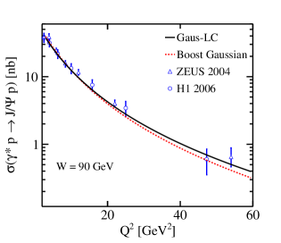
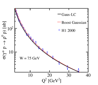
Figure 5: (Left) Prediction for cross section of $\gamma^{*}p\rightarrow J/\Psi p$ as a function of $Q^{2}$ with two different meson wave functions compared with experimental data from ZEUS 2004 Chekanov et al. (2004) and H1 2006 Aktas et al. (2006). (Right) Total cross sections of $\gamma^{*}p\rightarrow\rho^{0}p$ as a function of $Q^{2}$ compared with experimental data from H1 2000 Adloff et al. (2000) using two different meson wave functions.

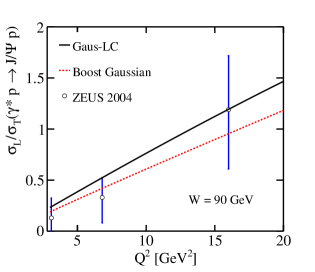
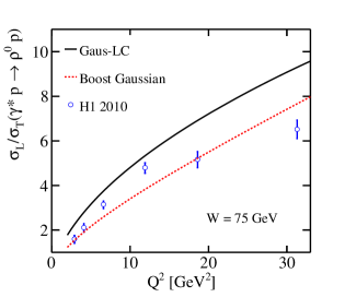
Figure 6: (Left) For $\gamma^{*}p\rightarrow J/\Psi p$, the ratio of $\sigma_{L}$ and $\sigma_{T}$ as a function of $Q^{2}$ with two different meson wave functions compared with experimental data from ZEUS 2004 Chekanov et al. (2004) when $\rm W\,=\,90\,\rm GeV$. (Right) For $\gamma^{*}p\rightarrow\rho^{0}p$, the ratio of $\sigma_{L}$ and $\sigma_{T}$ as a function of $Q^{2}$ compared with experimental data from H1 2010 Aaron et al. (2010a) using two different meson wave functions, when $\rm W\,=\,75\,\rm GeV$.

III analytical solution of BK equation

In addition to wave functions, dipole-target scattering amplitude also determines exclusive vector meson production process. In $\left|\mathcal{A}_{T,L}^{\gamma^{*}p\rightarrow Vp}\right|_{t=0}$ of Eq.  (6), dipole scattering differential cross section $\mathrm{d}\sigma_{q\bar{q}}/\mathrm{d}^{2}\bm{b}$ is integrated and written as

$$\int\frac{\mathrm{~{}d}\sigma_{q\bar{q}}}{\mathrm{~{}d}^{2}\bm{b}}(x,r,\bm{b})\mathrm{d}^{2}\bm{b}=\sigma_{q\bar{q}}(x,r)=2\pi R_{p}^{2}N(x,r),$$ (13)

where $R_{p}$ is proton radius which will be obtained by fitting with structure function $F_{2}$ data of proton from DIS process, and the scattering amplitude $N(x,r)$ comes from BK equation.

In the momentum space, with proper approximation, BK equation is represented as a nonlinear evolution equation Munier and Peschanski (2003)

$$\frac{\partial\mathcal{N}(\rm k,\rm Y)}{\partial\rm Y}= \frac{\alpha_{\mathrm{s}}N_{\mathrm{c}}}{\pi}\chi\left(-\frac{\partial}{\partial\ln\rm k^{2}}\right)\mathcal{N}(\rm k,\rm Y)$$ (14)

$$-\frac{\alpha_{\mathrm{s}}N_{\mathrm{c}}}{\pi}\mathcal{N}^{2}(\rm k,\rm Y),$$

where $\chi(\lambda)=\psi(1)-\frac{1}{2}\psi\left(1-\frac{\lambda}{2}\right)-\frac{1}{2}\psi\left(\frac{\lambda}{2}\right)$ is BFKL kernel with $\psi(\lambda)=\Gamma^{\prime}(\lambda)/\Gamma(\lambda)$. In addition, $\rm Y=ln$$\frac{1}{x}$.

When fixing the running strong coupling constant and expanding the BFKL kernel $\chi(\lambda)$ Marquet et al. (2005), we obtain

$$A_{0}\mathcal{N}-\mathcal{N}^{2}-\frac{\partial\mathcal{N}}{\partial\rm Y}-A_{1}\frac{\partial\mathcal{N}}{\partial\rm L}+\sum_{p=2}^{P}(-1)^{p}A_{p}\frac{\partial^{p}\mathcal{N}}{\partial^{p}\rm L}=0.$$ (15)

Here, we need to clarify that the unit of $\rm Y$ is $\bar{\alpha}_{s}=\frac{\alpha_{s}N_{c}}{\pi}$, and $\rm L=\rm ln\,k^{2}/k^{2}_{0}$. For the calculation, we have fixed $\bar{\alpha}_{s}=0.191$ and $\rm k^{2}_{0}=\Lambda^{2}_{\rm QCD}=0.04\,\rm GeV^{2}$. With $P=2$, the simplified BK equation is given by

$$A_{0}\mathcal{N}-\mathcal{N}^{2}-\frac{\partial\mathcal{N}}{\partial\rm Y}-A_{1}\frac{\partial\mathcal{N}}{\partial\rm L}+A_{2}\frac{\partial^{2}\mathcal{N}}{\partial^{2}\rm L}=0.$$ (16)

The analytical solutions of Eq.  (16) has be given as Wang et al. (2021)

$$\mathcal{N}(\rm L,Y)=\frac{A_{0}e^{5A_{0}\rm Y/3}}{\left[e^{5A_{0}\rm Y/6}+e^{\left[-\theta+\sqrt{A_{0}/6A_{2}}\left(\rm L-A_{1}\rm Y\right)\right]}\right]^{2}}.$$ (17)

In this work, the values of $\rm A_{0}$, $\rm A_{1}$, $\rm A_{2}$ and $\theta$ are given by fitting to proton structure function $F_{2}$ with the following relationship between $F_{2}$ and $\mathcal{N}(L,Y)$ de Santana Amaral et al. (2007):

$$F_{2}\left(x,Q^{2}\right)=\frac{Q^{2}R_{p}^{2}N_{c}}{4\pi^{2}}\int_{0}^{\infty}\frac{d\rm{k}}{\rm{k}}\int_{0}^{1}dz\left|\tilde{\Psi}_{\gamma}\left(\rm{k^{2}},z;Q^{2}\right)\right|^{2}\mathcal{N}(\rm L,Y),$$ (18)

where $N_{c}$ is the number of colors. Here $x\,=\,x_{Bj}$. As shown in Fig. 1 (Left), the wave function $\left|\tilde{\Psi}_{\gamma}\left(\rm{k^{2}},z;Q^{2}\right)\right|^{2}$ expressed in momentum space, represents the probability of a virtual photon splitting into a quark-antiquark pair. It is given by de Santana Amaral et al. (2007)

$$\left|\tilde{\Psi}_{\gamma}\left({\rm k^{2}},z;Q^{2}\right)\right|^{2} =\sum_{q}\left(\frac{4\bar{Q}_{q}^{2}}{{\rm k^{2}}+4\bar{Q}_{q}^{2}}\right)^{2}e_{q}^{2}\left.\bigg{\{}\left[z^{2}+(1-z)^{2}\right]\right.$$ (19)

$$\times\left[\frac{4\left({\rm k^{2}}+\bar{Q}_{q}^{2}\right)}{\sqrt{{\rm k^{2}}\left({\rm k^{2}}+4\bar{Q}_{q}^{2}\right)}}\operatorname{arcsinh}\left(\frac{{\rm k}}{2\bar{Q}_{q}}\right)\right.$$

$$\left.+\frac{{\rm k^{2}}-2\bar{Q}_{q}^{2}}{2\bar{Q}_{q}^{2}}\right]+\frac{4Q^{2}z^{2}(1-z)^{2}+m_{q}^{2}}{\bar{Q}_{q}^{2}}$$

$$\times\left[\frac{{\rm k^{2}}+\bar{Q}_{q}^{2}}{\bar{Q}_{q}^{2}}-\frac{4\bar{Q}_{q}^{4}+2\bar{Q}_{q}^{2}{\rm k^{2}+k^{4}}}{\bar{Q}_{q}^{2}\sqrt{{\rm k^{2}}\left({\rm k^{2}}+4\bar{Q}_{q}^{2}\right)}}\right.$$

$$\left.\left.\times\operatorname{arcsinh}\left(\frac{{\rm k}}{2\bar{Q}_{q}}\right)\right]\right.\bigg{\}},$$

where $\bar{Q}_{q}^{2}=z(1-z)Q^{2}+m_{q}^{2}$, $m_{q}$ the mass of the quark of flavor $q$.

In de Santana Amaral et al. (2007), their fitting range for $Q^{2}$ is $0.045\,\leq Q^{2}\leq 150\,\mathrm{GeV}^{2}$, because the corrections from DGLAP equation should be considered in too high $Q^{2}$ range. So the kinematic fitting range we choose is

$$\begin{gathered}x\,\leq\,0.01,\\ 1\,\mathrm{GeV}^{2}\,<\,Q^{2}\,\leq\,45\,\mathrm{GeV}^{2}.\end{gathered}$$ (20)

The fitting results are presented in Fig. $\ref{fig:F19},\,\ref{fig:F20}$. the values of the parameters obtained by fitting to 85 $F_{2}$ data points from H1 and ZEUS Aaron et al. (2010b); Andreev et al. (2014) with $m_{u,d,s}\,=\,0.14\,\rm GeV$ and $m_{c}\,=\,1.4\,\rm GeV$ are listed in table. 1. The $\chi^{2}$ is also provided in table. 1 .

Table 1: Parameters from the fit to the $F_{2}$ data Aaron et al. (2010b); Andreev et al. (2014) and $\chi^{2}$ per data points (nop means “number of points”).

$x$	$Q^{2}/\rm\,GeV^{2}$	$m_{u,d,s}/\,\rm GeV$	$m_{c}/\,\rm GeV$	$\alpha_{s}$	$\rm k_{0}/\,\rm GeV$	$\rm A_{0}$	$\rm A_{1}$	$\rm A_{2}$	$\theta$	$R_{p}/\,\rm GeV^{-1}$	$\chi^{2}/{\rm nop}$
$\leq\,0.01$	$(1,45]$	0.14	1.4	0.2	0.2	$0.696\,\pm\,0.0187$	$0.661\,\pm\,0.0295$	$0.112\,\pm\,8.0\times 10^{-3}$	$-0.463\,\pm\,0.0493$	$5.484\,\pm\,0.106$	0.979

Then in the following calculation, we need the dipole scattering amplitude $\mathcal{N}(x,\textbf{r})$ in the coordinate space. $\mathcal{N}(x,\textbf{r})$ is related to $\mathcal{N}(x,\textbf{k})$ by the Fourier transformation,

$$\mathcal{N}(x,\textbf{k})=\frac{1}{2\pi}\int\frac{d^{2}\textbf{r}}{r^{2}}e^{i\textbf{k}\cdot\textbf{r}}\mathcal{N}(x,\textbf{r}).$$ (21)

By inverse Fourier transformation, we can get

$$\mathcal{N}(x,\textbf{r}) =\frac{r^{2}}{2\pi}\int{d^{2}\textbf{k}}e^{-i\textbf{k}\cdot\textbf{r}}\mathcal{N}(x,\textbf{k})$$ (22)

$$=r^{2}\int^{\infty}_{0}dkkJ_{0}(k\cdot r)\mathcal{N}(x,k).$$

Then, we apply Eq.  (22) to the total cross section calculations of $J/\Psi$ and $\rho^{0}$ productions.

IV Numerical results

The cross sections of vector mesons are calculated with the dipole-amplitude and overlaps between the vector meson and the photon wave functions. In this work, the wave functions of vector mesons are adopted in two models. The solution of BK equation in previous section is employed for dipole-amplitude. We examine whether the solution of BK equation is valid in the calculations.

We present the differential cross sections, total cross sections and ratios of $\sigma_{L}$ and $\sigma_{T}$ of $\rho^{0}$ and $J/\Psi$ productions respectively using our analytic solution of BK equation. For the wave functions of the total cross section, we consider the influence of the “Gaus-LC” model and the “boosted Gaussian” model respectively. Finally, the total cross sections are calculated theoretically and compared with the experimental data.

First of all, the results of differential cross sections of $J/\Psi$ and $\rho^{0}$ productions as a function of t are presented compared with experiment data Aktas et al. (2006); Chekanov et al. (2004, 2007); Aaron et al. (2010a), as shown in Fig.  3. Then we predict the $\rm W$-dependence total cross sections of two meson in two wave functions models with our solutions of BK equation. As shown in Fig.  4, for exclusive $J/\Psi$ and $\rho^{0}$ productions, we compare our results with the experimental data Chekanov et al. (2004); Aktas et al. (2006); Adloff et al. (2000); Chekanov et al. (2007), in the case of $7.0\,\rm GeV^{2}\leq Q^{2}\leq 22.4\,\rm GeV^{2}$ and $8.3\,\rm GeV^{2}\leq Q^{2}\leq 32.0\,\rm GeV^{2}$. From the results, the calculations are reasonable within the range of uncertainty allowed. And we can find the results obtained by “Gaus-LC” model and “boosted Gaussian” model become closing to each other as $Q^{2}$ increasing. For $J/\Psi$, total cross sections obtained by two models are even flip-over at higher $Q^{2}$. These are mainly from the contribution of the wave functions. As shown in Fig. 2, for transversely polarized part of $\rho^{0}$ and $J/\Psi$, the difference between the two models is gradually reduced as $Q^{2}$ increases. For longitudinally polarized part of $\rho^{0}$, the two models are basically the same. But for $J/\Psi$, There are some differences between the two models.

Secondly, the total cross sections as a function of $Q^{2}$ are presented in Fig.  5 when $\rm W=90\,\rm GeV$ for $J/\Psi$ and $\rm W=75\,\rm GeV$ for $\rho^{0}$. It can be seen that the predictions agree with the experimental data well. Then, to summarize, the solution of BK equation is valid to perform the cross sections of vector meson in diffractive process.

Thirdly, Fig.  6 shows the ratios of the longitudinal to transverse cross section, $\sigma_{L}/\sigma_{T}$ as a function of $Q^{2}$ for fixed $\rm W$. For $J/\Psi$ production, $\sigma_{L}/\sigma_{T}\,\propto Q^{2}$. And for $\gamma^{*}p\rightarrow\rho^{0}p$ process, $\sigma_{L}/\sigma_{T}$ based on two wave function models grows rapidly with $Q^{2}$. As $Q^{2}$ increases, the ratio calculated by us exceeds the experimental data. In Kowalski et al. (2006), a reasonable explanation is given for this situation. The ratios of the longitudinal to transverse cross section are sensitive to the wave functions.

Briefly, when the running coupling constant $\alpha_{s}$ is fixed, the solution of BK equation with the parameters fitted by us in this work is efficient in the prediction of the meson production. As $Q^{2}$ increases , $\alpha_{s}$ vanishes asymptotically. Only at large $Q^{2}$, we can assume that its dependence on $Q^{2}$ diminishes. Accordingly, the $F_{2}$ data of $Q^{2}\,<\,1\,\rm GeV^{2}$ is not considered. And too high $Q^{2}$ data is also not taken into account, because the DGLAP corrections could work in too high $Q^{2}$ region de Santana Amaral et al. (2007).

V Discussion and Summary

In this work, the good values of parameters in the solution of BK equation are obtained by fitting the $F_{2}$ data firstly. Then we use the solution of BK equation and two wave function models (the “Gaus-LC” model and the “boosted Gaussian” model) to get the total cross sections of the exclusive $\rho^{0}$ and $J/\psi$ productions and the ratios of the longitudinal to transverse cross section. The results show that the analytical solution of BK equation with fixed $\alpha_{s}$ is suitable within a certain $Q^{2}$ region. And the difference of the results caused by the two wave function models decreases with the increase of $Q^{2}$ for $\rho^{0}$. But for $J/\Psi$, at higher $Q^{2}$, the difference still occurs.

To be more precise, our solution of BK equation with the parameters fitted by us is valid within not too high $Q^{2}$ region. If this region is exceeded, it may be more appropriate to use the DGLAP equation or improved BK equation Albacete (2017); Albacete et al. (2009).

In a word, vector meson production is effective to measure the properties of proton. In the future, EIC Abdul Khalek et al. (2021) and EicC Anderle et al. (2021) experimental data will offer more tests on BK equation.

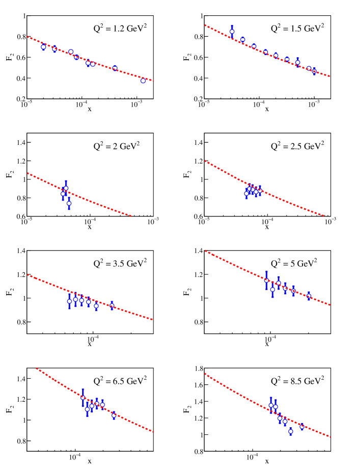
Figure 7: Result for fitting to proton structure function $F_{2}$ as a function of $x$ at different $Q^{2}$. These data are from H1 and ZEUS Aaron et al. (2010b); Andreev et al. (2014). The red dotted line is the fitting curve by eq. (18).

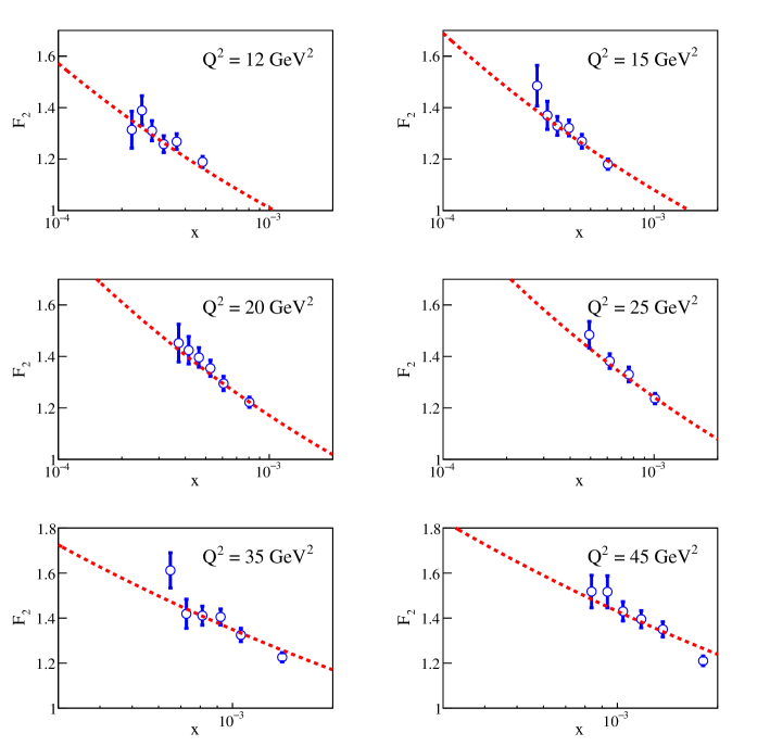
Figure 8: Continuation of Fig. 7.

References

- McLerran and Venugopalan (1994) L. D. McLerran and R. Venugopalan, Phys. Rev. D 49, 2233 (1994), arXiv:hep-ph/9309289 .
- Iancu et al. (2002) E. Iancu, A. Leonidov, and L. McLerran, in Cargese Summer School on QCD Perspectives on Hot and Dense Matter (2002) pp. 73–145, arXiv:hep-ph/0202270 .
- Iancu and Venugopalan (2003) E. Iancu and R. Venugopalan, “The Color glass condensate and high-energy scattering in QCD,” in Quark-gluon plasma 4, edited by R. C. Hwa and X.-N. Wang (2003) pp. 249–3363, arXiv:hep-ph/0303204 .
- Jalilian-Marian and Kovchegov (2006) J. Jalilian-Marian and Y. V. Kovchegov, Prog. Part. Nucl. Phys. 56, 104 (2006), arXiv:hep-ph/0505052 .
- Gelis et al. (2010) F. Gelis, E. Iancu, J. Jalilian-Marian, and R. Venugopalan, Ann. Rev. Nucl. Part. Sci. 60, 463 (2010), arXiv:1002.0333 [hep-ph] .
- Gribov et al. (1983) L. V. Gribov, E. M. Levin, and M. G. Ryskin, Phys. Rept. 100, 1 (1983).
- Mueller and Qiu (1986) A. H. Mueller and J.-w. Qiu, Nucl. Phys. B 268, 427 (1986).
- Mueller (1999) A. H. Mueller, Nucl. Phys. B 558, 285 (1999), arXiv:hep-ph/9904404 .
- Nikolaev and Zakharov (1991) N. N. Nikolaev and B. G. Zakharov, Z. Phys. C 49, 607 (1991).
- Mueller and Patel (1994) A. H. Mueller and B. Patel, Nucl. Phys. B 425, 471 (1994), arXiv:hep-ph/9403256 .
- Mueller (1994) A. H. Mueller, Nucl. Phys. B 415, 373 (1994).
- Kopeliovich and Zakharov (1991) B. Z. Kopeliovich and B. G. Zakharov, Phys. Rev. D 44, 3466 (1991).
- Kopeliovich et al. (1994) B. Z. Kopeliovich, J. Nemchick, N. N. Nikolaev, and B. G. Zakharov, Phys. Lett. B 324, 469 (1994), arXiv:hep-ph/9311237 .
- Nemchik et al. (1994) J. Nemchik, N. N. Nikolaev, and B. G. Zakharov, Phys. Lett. B 341, 228 (1994), arXiv:hep-ph/9405355 .
- Nemchik et al. (1996) J. Nemchik, N. N. Nikolaev, E. Predazzi, and B. G. Zakharov, Phys. Lett. B 374, 199 (1996), arXiv:hep-ph/9604419 .
- Nemchik et al. (1997) J. Nemchik, N. N. Nikolaev, E. Predazzi, and B. G. Zakharov, Z. Phys. C 75, 71 (1997), arXiv:hep-ph/9605231 .
- Golec-Biernat and Wusthoff (1998) K. J. Golec-Biernat and M. Wusthoff, Phys. Rev. D 59, 014017 (1998), arXiv:hep-ph/9807513 .
- Iancu et al. (2004) E. Iancu, K. Itakura, and S. Munier, Phys. Lett. B 590, 199 (2004), arXiv:hep-ph/0310338 .
- Watt and Kowalski (2008) G. Watt and H. Kowalski, Phys. Rev. D 78, 014016 (2008), arXiv:0712.2670 [hep-ph] .
- Kowalski et al. (2006) H. Kowalski, L. Motyka, and G. Watt, Phys. Rev. D 74, 074016 (2006), arXiv:hep-ph/0606272 .
- Kowalski and Teaney (2003) H. Kowalski and D. Teaney, Phys. Rev. D 68, 114005 (2003), arXiv:hep-ph/0304189 .
- Rezaeian et al. (2013) A. H. Rezaeian, M. Siddikov, M. Van de Klundert, and R. Venugopalan, Phys. Rev. D 87, 034002 (2013).
- Lappi and Mantysaari (2011) T. Lappi and H. Mantysaari, Phys. Rev. C 83, 065202 (2011), arXiv:1011.1988 [hep-ph] .
- Kowalski et al. (2008a) H. Kowalski, T. Lappi, and R. Venugopalan, Phys. Rev. Lett. 100, 022303 (2008a), arXiv:0705.3047 [hep-ph] .
- Kowalski et al. (2008b) H. Kowalski, T. Lappi, C. Marquet, and R. Venugopalan, Phys. Rev. C 78, 045201 (2008b), arXiv:0805.4071 [hep-ph] .
- Xie and Goncalves (2022) Y.-P. Xie and V. P. Goncalves, Phys. Rev. D 105, 014033 (2022), arXiv:2201.10499 [hep-ph] .
- Fadin et al. (1975) V. S. Fadin, E. A. Kuraev, and L. N. Lipatov, Phys. Lett. B 60, 50 (1975).
- Kuraev et al. (1976) E. A. Kuraev, L. N. Lipatov, and V. S. Fadin, Sov. Phys. JETP 44, 443 (1976).
- Kuraev et al. (1977) E. A. Kuraev, L. N. Lipatov, and V. S. Fadin, Sov. Phys. JETP 45, 199 (1977).
- Balitsky and Lipatov (1978) I. I. Balitsky and L. N. Lipatov, Sov. J. Nucl. Phys. 28, 822 (1978).
- Gribov and Lipatov (1972) V. N. Gribov and L. N. Lipatov, Sov. J. Nucl. Phys. 15, 438 (1972).
- Dokshitzer (1977) Y. L. Dokshitzer, Sov. Phys. JETP 46, 641 (1977).
- Altarelli and Parisi (1977) G. Altarelli and G. Parisi, Nucl. Phys. B 126, 298 (1977).
- Rezaeian and Schmidt (2013) A. H. Rezaeian and I. Schmidt, Phys. Rev. D 88, 074016 (2013), arXiv:1307.0825 [hep-ph] .
- Motyka and Watt (2008) L. Motyka and G. Watt, Phys. Rev. D 78, 014023 (2008), arXiv:0805.2113 [hep-ph] .
- Levin and Rezaeian (2010) E. Levin and A. H. Rezaeian, Phys. Rev. D 82, 014022 (2010), arXiv:1005.0631 [hep-ph] .
- Tribedy and Venugopalan (2011) P. Tribedy and R. Venugopalan, Nucl. Phys. A 850, 136 (2011), [Erratum: Nucl.Phys.A 859, 185–187 (2011)], arXiv:1011.1895 [hep-ph] .
- Xie and Chen (2018) Y.-P. Xie and X. Chen, Nucl. Phys. A 970, 316 (2018), arXiv:1805.06210 [hep-ph] .
- Balitsky (1997) I. Balitsky, AIP Conf. Proc. 407, 953 (1997), arXiv:hep-ph/9706411 .
- Kovchegov (1999) Y. V. Kovchegov, Phys. Rev. D 60, 034008 (1999), arXiv:hep-ph/9901281 .
- Kovchegov (2000) Y. V. Kovchegov, Phys. Rev. D 61, 074018 (2000), arXiv:hep-ph/9905214 .
- Balitsky (2001) I. Balitsky, Phys. Lett. B 518, 235 (2001), arXiv:hep-ph/0105334 .
- Balitsky (1996) I. Balitsky, Nucl. Phys. B 463, 99 (1996), arXiv:hep-ph/9509348 .
- Jalilian-Marian et al. (1997) J. Jalilian-Marian, A. Kovner, A. Leonidov, and H. Weigert, Nucl. Phys. B 504, 415 (1997), arXiv:hep-ph/9701284 .
- Iancu et al. (2001) E. Iancu, A. Leonidov, and L. D. McLerran, Nucl. Phys. A 692, 583 (2001), arXiv:hep-ph/0011241 .
- Weigert (2002) H. Weigert, Nucl. Phys. A 703, 823 (2002), arXiv:hep-ph/0004044 .
- Golec-Biernat and Stasto (2003) K. J. Golec-Biernat and A. M. Stasto, Nucl. Phys. B 668, 345 (2003), arXiv:hep-ph/0306279 .
- Bendova et al. (2019) D. Bendova, J. Cepila, J. G. Contreras, and M. Matas, Phys. Rev. D 100, 054015 (2019), arXiv:1907.12123 [hep-ph] .
- Matas et al. (2016) M. Matas, J. Cepila, and J. Guillermo Contreras Nuno, EPJ Web Conf. 112, 02008 (2016).
- Lappi and Mäntysaari (2015) T. Lappi and H. Mäntysaari, Phys. Rev. D 91, 074016 (2015), arXiv:1502.02400 [hep-ph] .
- Munier and Peschanski (2003) S. Munier and R. B. Peschanski, Phys. Rev. Lett. 91, 232001 (2003), arXiv:hep-ph/0309177 .
- Munier and Peschanski (2004a) S. Munier and R. B. Peschanski, Phys. Rev. D 69, 034008 (2004a), arXiv:hep-ph/0310357 .
- Munier and Peschanski (2004b) S. Munier and R. B. Peschanski, Phys. Rev. D 70, 077503 (2004b), arXiv:hep-ph/0401215 .
- Fisher (1937) R. A. Fisher, Annals of Human Genetics 7, 355 (1937).
- Bondarenko and Prygarin (2015) S. Bondarenko and A. Prygarin, JHEP 06, 090 (2015), arXiv:1503.05437 [hep-ph] .
- Marquet et al. (2005) C. Marquet, R. B. Peschanski, and G. Soyez, Phys. Lett. B 628, 239 (2005), arXiv:hep-ph/0509074 .
- Xiang et al. (2017) W. Xiang, S. Cai, and D. Zhou, Phys. Rev. D 95, 116009 (2017), arXiv:1701.07378 [hep-ph] .
- Xiang et al. (2020) W. Xiang, Y. Cai, M. Wang, and D. Zhou, Phys. Rev. D 101, 076005 (2020), arXiv:1911.06744 [hep-ph] .
- Xiang et al. (2021) W.-C. Xiang, M.-L. Wang, Y.-B. Cai, and D.-C. Zhou, Chin. Phys. C 45, 014103 (2021), arXiv:2008.04235 [hep-ph] .
- Wang et al. (2021) X. Wang, Y. Yang, W. Kou, R. Wang, and X. Chen, Phys. Rev. D 103, 056008 (2021), arXiv:2009.13325 [hep-ph] .
- Forshaw et al. (2004) J. R. Forshaw, R. Sandapen, and G. Shaw, Phys. Rev. D 69, 094013 (2004), arXiv:hep-ph/0312172 .
- Shuvaev et al. (1999) A. G. Shuvaev, K. J. Golec-Biernat, A. D. Martin, and M. G. Ryskin, Phys. Rev. D 60, 014015 (1999), arXiv:hep-ph/9902410 .
- Ahmady et al. (2016) M. Ahmady, R. Sandapen, and N. Sharma, Phys. Rev. D 94, 074018 (2016), arXiv:1605.07665 [hep-ph] .
- Cepila et al. (2019) J. Cepila, J. Nemchik, M. Krelina, and R. Pasechnik, Eur. Phys. J. C 79, 495 (2019), arXiv:1901.02664 [hep-ph] .
- Chekanov et al. (2002) S. Chekanov et al. (ZEUS), Eur. Phys. J. C 24, 345 (2002), arXiv:hep-ex/0201043 .
- Chekanov et al. (2004) S. Chekanov et al. (ZEUS), Nucl. Phys. B 695, 3 (2004), arXiv:hep-ex/0404008 .
- Aktas et al. (2006) A. Aktas et al. (H1), Eur. Phys. J. C 46, 585 (2006), arXiv:hep-ex/0510016 .
- Chekanov et al. (2007) S. Chekanov et al. (ZEUS), PMC Phys. A 1, 6 (2007), arXiv:0708.1478 [hep-ex] .
- Aaron et al. (2010a) F. D. Aaron et al. (H1), JHEP 05, 032 (2010a), arXiv:0910.5831 [hep-ex] .
- Adloff et al. (2000) C. Adloff et al. (H1), Eur. Phys. J. C 13, 371 (2000), arXiv:hep-ex/9902019 .
- de Santana Amaral et al. (2007) J. T. de Santana Amaral, M. B. Gay Ducati, M. A. Betemps, and G. Soyez, Phys. Rev. D 76, 094018 (2007), arXiv:hep-ph/0612091 .
- Aaron et al. (2010b) F. D. Aaron et al. (H1, ZEUS), JHEP 01, 109 (2010b), arXiv:0911.0884 [hep-ex] .
- Andreev et al. (2014) V. Andreev et al. (H1), Eur. Phys. J. C 74, 2814 (2014), arXiv:1312.4821 [hep-ex] .
- Albacete (2017) J. L. Albacete, Nucl. Phys. A 957, 71 (2017), arXiv:1507.07120 [hep-ph] .
- Albacete et al. (2009) J. L. Albacete, N. Armesto, J. G. Milhano, and C. A. Salgado, Phys. Rev. D 80, 034031 (2009), arXiv:0902.1112 [hep-ph] .
- Abdul Khalek et al. (2021) R. Abdul Khalek et al., (2021), arXiv:2103.05419 [physics.ins-det] .
- Anderle et al. (2021) D. P. Anderle et al., Front. Phys. (Beijing) 16, 64701 (2021), arXiv:2102.09222 [nucl-ex] .