Searching for velocity-dependent dark matter annihilation signals from extragalactic halos

Abstract

We consider gamma-ray signals of dark matter annihilation in extragalactic halos in the case where dark matter annihilates from a $p$-wave or $d$-wave state. In these scenarios, signals from extragalactic halos are enhanced relative to other targets, such as the Galactic Center or dwarf spheroidal galaxies, because the typical relative speed of the dark matter is larger in extragalactic halos. We perform a mock data analysis of gamma rays produced by dark matter annihilation in halos detected by the Sloan Digital Sky Survey. We include a model for uncorrelated galactic and extragalactic gamma ray backgrounds, as well as a simple model for backgrounds due to astrophysical processes in the extragalactic halos detected by the survey. We find that, for models which are still allowed by other gamma ray searches, searches of extragalactic halos with the current Fermi exposure can produce evidence for dark matter annihilation, though it is difficult to distinguish the $p$-wave and $d$-wave scenarios. With a factor $10\times$ larger exposure, though, discrimination of the velocity-dependence is possible.

1 Introduction

A promising strategy in dark matter indirect detection is the search for photons produced by dark matter annihilation in astrophysical objects with a large dark matter density. This strategy is particularly fruitful because the photons point back to their source, allowing one to use prior information about the dark matter distribution to enhance detection prospects. For example, some of the best sensitivity to dark matter annihilation arises from searches for high energy photons arriving from the direction of dwarf spheroidal galaxies (dSphs) [1, 2, 3, 4] or from the Milky Way Galactic Center (GC) [5, 6, 7, 8, 9], which are localized on the sky, are thought to have large dark matter densities, and are relatively nearby.

Extragalactic dark matter halos also contain large amounts of dark matter, and can be localized with observations of the galaxies that they host, gravitational lensing, and other techniques. Relative to dSphs, the larger masses of extragalactic halos and their larger distances push the annihilation signal in opposite directions, leading to a total expected flux from known extragalactic halos that is similar to that from known dSphs in standard dark matter annihilation models. To date, however, extragalactic dark matter halos have not provided constraints on the dark matter annihilation cross section that are competitive with those from dSphs. There are two primary reasons for this. First, dSphs take up a smaller sky fraction than extragalactic halos, meaning that the total background contribution for dSphs is significantly smaller. Second, dSphs are expected to have smaller correlated astrophysical backgrounds since there are few conventional gamma-ray producing sources inside of these dark matter-dominated objects. Extragalactic halos, on the other hand, can be powerful emitters of gamma-rays via non-dark matter processes [e.g. Ref. 12], making separating signal from background challenging (see further discussion of observational challenges of detecting annihilation radiation from extragalactic halos in Refs. [13, 14, 15]).

However, in dark matter models where the velocity-weighted annihilation cross section is velocity-dependent, the signal from extragalactic halos can be greatly enhanced relative to that from dSphs. Our particular focus is on scenarios in which the dark matter annihilation only occurs from a $p$-wave or $d$-wave initial state, scenarios realized in a variety of well-motivated theoretical models. If dark matter annihilation is $p$-wave or $d$-wave suppressed, then the annihilation cross section is suppressed by factors of $(v/c)^{2}$ or $(v/c)^{4}$, respectively, where $v$ is the relative velocity of the dark matter particles. Searches of large extragalactic halos are particularly interesting in this case, because the relative velocities of dark matter particles in these halos tend to be larger than in targets within the Milky Way, implying that the signal from extragalactic halos is enhanced relative to that from dSphs or the GC for $p$-/$d$-wave suppressed dark matter annihilation. Previous studies of velocity-dependent dark matter annihilation in extragalactic dark matter halos include Refs. [16, 17].

The scenario of $p$-wave or $d$-wave annihilation is especially interesting in the context of the Galactic Center (GC) excess [5, 6]. This excess of GeV-range photons has been studied in the context of $s$-wave dark matter annihilation, where it is found that models which would be consistent with the GC excess are roughly at the limit of current bounds from searches for gamma rays from dwarf spheroidal galaxies (see, for example Refs. [18, 19]). But in models of $p$- or $d$-wave annihilation, the constraints from dSphs are weakened relative to those from the GC, because relative particle speeds tend to be smaller in dSphs, yielding reduced annihilation rates [20]. As a result, the scenario of $p$- or $d$-wave annihilation would weaken constraints from dSphs on dark matter explanations of the GC excess. But since these scenarios yield enhanced annihilation rates in extragalactic halos, those become an important search target for exploring explanations of the GC excess.

In this paper, we perform an idealized mock analysis to explore the prospects for detecting and characterizing the annihilation signal from extragalactic dark matter halos in models where the annihilation cross section is $p$-wave or $d$-wave suppressed. We generate mock gamma-ray data using a catalog of real halos detected by the Sloan Digital Sky Survey, and analyze this data using a template-based approach. While our approach is highly idealized compared to an analysis of real data, it suffices to determine the information content that could conceivably be extracted about $p$- and $d$-wave dark matter annihilation from current and future gamma-ray data sets. We will find that the simple intuition from above holds: in the idealized scenarios considered here, analyzing the extragalactic dark matter signal yields significantly tighter constraints on these models than analyses of dSphs. We find that this result is at least somewhat robust to freedom in background models.

The plan of this paper is as follows. In §2 we describe the catalog of extragalactic halos we use in our analysis; in §3 we describe our model for the dark matter annihilation signal; we describe the creation of a mock data set in §4, and the results of analyzing this data are described in §5. We conclude in §6.

2 Catalog of Extragalactic Dark Matter Halos

For the purposes of generating mock data, we rely on a catalog of dark matter halos detected in real data. Massive dark matter halos host galaxies, making galaxy surveys a powerful tool for identifying and localizing halos. By identifying galaxies that live in close proximity to one another via a spectroscopic survey, one can assign galaxies to groups, i.e. collections of galaxies that live in the same dark matter halo. In order to estimate the amplitude of the annihilation signal from each halo, we must have some knowledge of the halo’s mass distribution and distance. To this end, halo masses can be estimated from a variety of techniques, such as weak lensing or clustering. The distance, on the other hand, can be computed from the halo’s redshift assuming a cosmological model.

In this analysis, we use the galaxy group/halo catalog presented in Ref. [21], which is based on data from the Sloan Digital Sky Survey (SDSS). This halo catalog uses a modified version of the algorithm introduced in Refs. [22, 23] to assign galaxies to groups and estimate halo masses. We describe the method here briefly and refer readers to Ref. [21] for more details. First, galaxies are assigned a preliminary group identification assuming that every galaxy lives in its own halo, with halo mass computed based on observational proxies including stellar mass and luminosity. Next, assuming the group is described by a Navarro-Frenk-White (NFW) profile [24], the estimated mass is then used to estimate a halo radius and velocity dispersion, and the group membership is updated. Halo centers are then recomputed using the updated group membership. Next, halo mass estimates are recomputed using abundance matching, and the process is repeated. Ref. [21] assumes the $\Lambda$CDM cosmological model favored by WMAP9 [25] when constructing their catalog.

In order to remove fluctuations in the halo abundance that are due to variations in survey depth, and to make our results less dependent on survey strategy, we impose a completeness requirement on the halo catalog. Ref. [21] find that their SDSS-based halo catalog is complete for halo masses above $M\gtrsim 10^{12.5}\,M_{\odot}/h$ out to $z\lesssim 0.13$, and we select halos that satisfy these conditions. The range of redshifts in the resulting catalog is then $0.006\lesssim z\lesssim 0.13$, with median $\tilde{z}=0.1$. The range of halo masses in the catalog is $5\times 10^{12}\lesssim M/M_{\odot}\lesssim 2\times 10^{15}$, with median $\tilde{M}=5\times 10^{12}M_{\odot}$. There are a total of 59198 halos in the catalog. The sky footprint of the resulting catalog is presented in Figure 1.

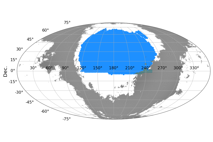
Figure 1: Sky footprint in equatorial coordinates of the halo catalog used in our analysis (blue). This catalog is from Ref. [21], and derived from SDSS data. Also shown in grey is the region of sky that is expected to have a galactic gamma-ray flux above the 75th percentile, as estimated using the model described in §3.4.

Our mock data set will miss contributions to the annihilation radiation that come from halos outside the mass and redshift bounds that we impose. Halos at higher redshifts will be largely uncorrelated with the halos in our catalog, and so are expected to act as a noise source for our analysis. We discuss our noise and background models in §3. Halos in the redshift range that we consider, but less massive than our mass cut, will produce a background of annihilation radiation that is correlated with the signal from high-mass halos. However, for the dark matter models that we consider, the fraction of annihilation radiation that we exclude is expected to be small. For the $n=2$ model considered below, our mass cut removes only about 10% of the expected annihilation luminosity at $z=0$, assuming the halo mass function from Ref. [10]; for the $n=4$ model, the mass cut removes less than 1% of the annihilation luminosity at $z=0$ (see further discussion of these points in §5.1).

3 Signals and Backgrounds

3.1 Expected annihilation flux from a dark matter halo

The flux of photons arising from dark matter annihilation in any dark matter halo can be expressed as

$$\Phi_{\rm DM} = \Phi_{PP}\times J,$$ (3.1)

where $\Phi_{PP}$ depends only on information about the dark matter particle physics, while $J$ (the $J$-factor) depends on the astrophysics of the target, and the velocity-dependence of the cross section. In particular,

$$\Phi_{PP} = \frac{(\sigma v)_{0}}{8\pi m_{X}^{2}}\times\int_{E_{\rm min}}^{E_{\rm max}}dE_{\gamma}~{}\frac{dN_{\gamma}}{dE_{\gamma}},$$

$$J = \frac{1}{D^{2}}\int d^{3}v_{1}\int d^{3}v_{2}~{}f(\vec{r}_{1},\vec{v}_{1})f(\vec{r}_{2},\vec{v}_{2})\times S(|\vec{v}_{1}-\vec{v}_{2}|/c),$$ (3.2)

where $m_{X}$ is the dark matter mass, $\sigma v=(\sigma v)_{0}\times S(v/c)$ is the dark matter annihilation cross section, $v$ is the relative velocity between dark matter particles, and $dN_{\gamma}/dE_{\gamma}$ is the energy spectrum of photons per annihilation (see, for example, [26]). The limits of the integral over $E_{\gamma}$ are restricted to $E_{\rm min}$ to $E_{\rm max}$, corresponding to the energy range of the detector. We assume that the dark matter particle is its own anti-particle. $D$ is the distance to the halo, and $f(\vec{r},\vec{v})$ is the dark matter velocity distribution function. The dark matter density distribution is then given by $\rho(\vec{r})=\int d^{3}v~{}f(\vec{r},\vec{v})$. Note, in writing Eq. 3.2, we have assumed that the size of the halo is much smaller than the distance $D$ to the halo. This is an excellent approximation for the extragalactic halos that we will consider.

We will assume that all extragalactic dark matter halos have velocity distributions which are spherically-symmetric and isotropic, and depend on only two parameters: a scale density $\rho_{s}$ and a scale radius $r_{s}$. We thus assume that each halo has a velocity-distribution which depends only on $r=|\vec{r}|$ and $v=|\vec{v}|$, and the velocity-distributions of two halos differ only by the values of the parameters $\rho_{s}$ and $r_{s}$. In reality, dark matter halos may have more complicated density and velocity distributions [e.g. 27], including the effects of triaxiality, velocity anisotropies, and detailed effects from baryonic physics. But we will see that these effects will not alter our overall conclusions, because the effect of their variation from halo to halo will be relatively small compared to that of the variation of the parameters $\rho_{s}$ and $r_{s}$. We note also that the supermassive black holes living at the centers of galaxies could result in changes to the dark matter distribution, and the formation of a dark matter ‘spike’ [28]; the impact of the velocity-dependent annihilation on such spikes has been considered in Refs. [29, 30].

We are interested in the case in which the velocity-dependence of the dark matter annihilation cross section is power-law ($S(v/c)=(v/c)^{n}$). The most interesting cases, for our purpose, are $p$-wave ($n=2$) and $d$-wave ($n=4$) annihilation, since the annihilation rate grows with relative velocity. Both of these examples are theoretically well-motivated. For example, dark matter annihilation will be $p$-wave if dark matter is a fermion which annihilates through an $s$-channel scalar interaction. $p$-wave annihilation can also be the dominant process if dark matter is a Majorana fermion which annihilates to a Standard Model fermion/anti-fermion pair through any interaction which respects minimal flavor violation (MFV) (see, for example, Ref. [31]). Similarly, $d$-wave annihilation may be the dominant process if dark matter is instead a real scalar particle [31, 32, 33]. Models with $n=1$ could arise in so-called ‘Impeded Dark Matter’ scenarios [34], but for simplicity, we will not consider that scenario here.

Under these assumptions, all of the dependence of the $J$-factor on the parameters can be determined by dimensional analysis [35]. In particular we find

$$J = \frac{4\pi M_{s}^{2}}{D^{2}r_{s}^{3}}\left(\frac{4\pi G_{N}M_{s}/r_{s}}{c^{2}}\right)^{n/2}\times\tilde{J}_{n}^{\rm tot},$$

$$= \frac{1.8~{}{\rm cm}^{-2}{\rm yr}^{-1}}{({\rm GeV}/c^{-2})^{-2}{\rm cm}^{3}{\rm s}^{-1}}\left[\frac{M_{s}}{M_{\odot}}\right]^{2}\left[\frac{r_{s}}{{\rm Mpc}}\right]^{-3}\left[\frac{D}{{\rm Mpc}}\right]^{-2}\left(6.1\times 10^{-19}\left[\frac{M_{s}}{M_{\odot}}\right]\left[\frac{r_{s}}{{\rm Mpc}}\right]^{-1}\right)^{n/2}$$

$$\times\tilde{J}_{n}^{\rm tot},$$

where $M_{s}\equiv\rho_{s}r_{s}^{3}$, and $\tilde{J}_{n}^{\rm tot}$ is a constant. The dependence of $J$ on $r_{s}$ and $M_{s}$ in Eq. 3.1, which determines our main results, will not depend on the functional form of the dark matter velocity distribution. The form of the velocity distribution will affect $\tilde{J}_{n}^{\rm tot}$, and this quantity has been estimated using a variety of techniques (for previous work on determining the $J$-factors for velocity-dependent dark matter matter annihilation, see [36, 37, 38, 26, 39, 40, 20, 41, 35, 42, 43]). But this is an overall normalization for the flux from all halos, which is degenerate with $\Phi_{PP}$. The relative magnitude of the fluxes from different halos depends only on the halo parameters $\rho_{s}$ and $r_{s}$, independent of the functional form of the halo density profile.

To determine $J$ then requires constraints on $D$, $M_{s}$, and $r_{s}$ for each halo. As mentioned previously, $D$ can be determined from the halo redshift assuming a cosmological model. However, the catalog of Ref. [21] does not provide independent measures of $M_{s}$ and $r_{s}$. Rather, total halo masses are inferred from an iterative process that assumes the distribution of galaxies in each halo follows an NFW profile with a fixed relation between $\rho_{s}$ and $r_{s}$. We will therefore adopt similar assumptions in our analysis.

The NFW density profile is given by

$$\rho(r) = \frac{\rho_{s}}{(r/r_{s})(1+(r/r_{s}))^{2}},$$ (3.4)

where $r_{s}$ and $\rho_{s}$ are parameters specific to each halo, as discussed above. The halo catalog of Ref. [21] adopts the spherical overdensity convention for defining halo mass. With this convention, the halo radius, $r_{\Delta,m/c}$, is defined such that the mass, $M_{\Delta,m/c}$, enclosed within $r_{\Delta,m/c}$ is a fixed multiple $\Delta$ of the (c)ritical or (m)ean density, $\rho_{m/c}$, of the Universe at the halo’s redshift, $z$:

$$M_{\rm halo}\equiv M_{\Delta,m/c}=\Delta\frac{4}{3}\pi r_{\Delta,m/c}^{3}\rho_{m/c}(z).$$ (3.5)

The halo catalog Ref. [21] uses $\Delta=180$ and $\rho_{m}$. The halo mass can be related to $M_{s}$ using the fact that

$$M_{\Delta,m/c} = 4\pi\int_{0}^{r_{\Delta,m/c}}dr~{}r^{2}~{}\rho(r),$$ (3.6)

$$= 4\pi M_{s}\left[\ln(1+c_{\Delta,m/c})+\frac{1}{1+c_{\Delta,m/c}}-1\right],$$

where we have defined the halo concentration parameter, $c_{\Delta,m/c}$, via $c_{\Delta,m/c}\equiv r_{\Delta,m/c}/r_{s}$. The mean relationship between $M_{\Delta,m/c}$ and $c_{\Delta,m/c}$ for NFW halos can be calibrated from CDM simulations. Here we use the relationship measured by Ref. [44] assuming $\Delta=200$:

$$c_{200,c}=A(M_{200,c}/M_{\rm pivot})^{B}(1+z)^{C}$$ (3.7)

where $M_{\rm pivot}=2\times 10^{12}\,h^{-1}M_{\odot}$, $A=5.71$, $B=-0.084$, $C=-0.47$; using an alternative concentration model, such as that from [45], results in a negligible change to our results. We now have a way to relate the halo masses reported by Ref. [21] to $M_{s}$ and $r_{s}$, thereby enabling computation of the $J$-factors, and thus the expected number of photons due to dark matter annihilation from each halo. We use the code Colossus [46] to convert between different halo mass definitions. Ignoring the distance dependence for simplicity, these relationships yield at $z=0$

$$J \propto \left[\frac{M_{s}}{M_{\odot}}\right]^{2+n/2}\left[\frac{r_{s}}{{\rm Mpc}}\right]^{-3-n/2}$$ (3.8)

$$\approx \left[0.55\times 10^{12}\,M_{\odot}\left(\frac{M_{180m}}{10^{13}\,M_{\odot}}\right)^{1.05}\right]^{2+n/2}\left[0.093\,{\rm Mpc}\left(\frac{M_{180m}}{10^{13}\,M_{\odot}}\right)^{0.415}\right]^{-3-n/2}$$ (3.9)

$$\propto M_{180m}^{0.86+0.32n}.$$ (3.10)

The above expression ignores scatter in the relationship between halo mass and concentration, which is known to exist as a result of the different assembly histories of halos [47]. Such scatter will in turn introduce scatter into the annihilation luminosities of the halos. However, this scatter is expected to be small. For example, Ref. [45] find that the scatter in the mass-concentration relation is roughly 0.16 dex, independent of halo mass, redshift and mass definition. This level of scatter is much smaller than than the variation in halo concentration across the range of halo masses that we consider. Similarly, in Ref. [48], it was found that the dark matter velocity dispersion has a power-law relationship with the halo mass, with very little scatter, for central halos found in Illustris simulations spanning more than three orders of magnitude in mass. Since the velocity dispersion is proportional to $(G_{N}M_{s}/r_{s})$, this corresponds to the statement that there is very little scatter in the $r_{s}-M_{s}$ relationship.

More generally, we have assumed that the functional form of the dark matter density profile depends only on the parameters $r_{s}$ and $M_{s}$. In order for either the mass-concentration relationship or the mass-velocity dispersion relationship to provide a power-law relationship between $M_{s}$ and $r_{s}$, one must necessarily introduce a new mass scale and a new length scale. These are effectively provided by $M_{\rm pivot}$ and $(M_{\rm pivot}/\rho_{m/c})^{1/3}$. In order for there to be scatter in either the mass-concentration relationship or the mass-velocity dispersion relationship, there would have to be another dimensionless parameter which could vary from halo to halo at fixed $z$. This parameter could then appear implicitly in the dark matter density profile; a triaxiality parameter would be an example of such a parameter. This would amount to a dependence of $\tilde{J}^{\rm tot}_{n}$ on some dimensionless parameter which varied from halo to halo. But the small magnitude of scatter in these relationships suggest that any additional dimensionless parameter only has a small variation over the halo mass range which we consider. Thus, we may treat $\tilde{J}^{\rm tot}_{n}$ as essentially constant, despite possible deviations in the halo velocity distribution from the form we have considered.

Finally, the number of photons expected due to dark matter annihilation in a halo characterized by the parameters $M_{s}$, $r_{s}$ and $D$ is

$$N_{\rm DM}^{({\rm halo})} = \Phi_{\rm DM}\times({\rm exposure}),$$ (3.11)

$$= 1.8\left[\frac{M_{s}}{M_{\odot}}\right]^{2}\left[\frac{r_{s}}{{\rm Mpc}}\right]^{-3}\left[\frac{D}{{\rm Mpc}}\right]^{-2}\left(6.1\times 10^{-19}\left[\frac{M_{s}}{M_{\odot}}\right]\left[\frac{r_{s}}{{\rm Mpc}}\right]^{-1}\right)^{n/2}$$

$$\times\tilde{J}_{n}^{\rm tot}\times\frac{(\rm exposure)}{{\rm cm}^{2}{\rm yr}}\times\frac{\Phi_{PP}}{({\rm GeV}/c^{2})^{-2}{\rm cm}^{3}{\rm s}^{-1}},$$

where, for halos described by NFW profiles (using Eddington inversion), one finds [35, 43]

$$\tilde{J}_{n=0}^{\rm tot}=0.33,\qquad\tilde{J}_{n=2}^{\rm tot}=0.14,\qquad\tilde{J}_{n=4}^{\rm tot}=0.12.$$ (3.12)

Note that other well-motivated profiles are possible (for reviews, see e.g. Refs. [49, 50]), and would yield different values of $\tilde{J}_{n}^{\rm tot}$. But the assumption of an NFW profile, and the choice of $\tilde{J}^{\rm tot}_{n}$, only affect the overall normalization of the flux, not the parametric dependence.

3.2 Boost factors

For this analysis, we assume that there is no boost factor enhancement of the photon flux due to substructure in the extragalactic halos. Estimates for the boost factor associated with extragalactic halos vary widely, from ${\cal O}(1)$ to a few orders of magnitude [51, 11]. But for our purposes, the important question is how the boost factor varies with halo mass. If the boost factor is constant, then it only yields an overall rescaling of the fluxes from all halos, which is degenerate with $\Phi_{PP}$.

If the extragalactic halo is really only characterized by two parameters, $\rho_{s}$ and $r_{s}$, then one would expect the boost factor to be essentially independent of halo mass, since there is no other dimensionless quantity which depends only on $G_{N}$, $\rho_{s}$ and $r_{s}$. This is consistent with results of Ref. [51], for example, in which it was found that, for a variety of models, the boost factor varies by about an order of magnitude as the halo mass varies over nine orders of magnitude.

We thus expect that our assumption of negligible boost factor will not have a major effect on the main results of our analysis. Note that, for $n>0$, we expect the effect of the boost factor to be even smaller because particles bound to subhalos tend to have smaller relative velocities (see, e.g., Ref. [16]). If $\sigma v$ grows with velocity, then the signal from subhalos will be suppressed relative to that from the central halo.

3.3 Extragalactic Anisotropic Background

Since galaxies can be powerful gamma-ray emitters, and since the halos in our sample host many galaxies, we expect these halos to emit gamma-rays not associated with dark matter annihilation. In addition to galactic gamma-rays, processes such as accretion shocks around galaxy clusters could also produce gamma-ray signals correlated with the halos in our sample [53]. These sources of gamma-rays constitute an important background for any search for gamma-ray photons produced by dark matter annihilation in extragalactic halos.

We will assume that future multi-wavelength observations can be used to identify and remove bright sources of known astrophysical (i.e. non-dark matter) origin. We additionally make the very simple assumption that the luminosity of the remaining astrophysical sources in an extragalactic halo is proportional to the halo mass. Since we will be analyzing mock data generated from this model, it is not necessary that this model be precisely correct. By assuming that the astrophysical gamma-ray emission is proportional to the halo mass, we build in the fact that large halos, which are likely to produce more photons from dark matter annihilation, are also likely to produce more photons from astrophysical processes. Furthermore, in an actual analysis on data, it may be possible to use multi-wavelength observations to infer the astrophysical (i.e. non-dark matter) emission from a catalog of halos. For example, for star forming galaxies, the star formation rate is expected to correlate with the gamma-ray luminosity; observations in the optical or infrared could therefore be used to place a prior on the gamma-ray luminosity of a halo [54]. Thus, while our assumed relation between astrophysical gamma-ray luminosity and halo mass is unlikely to be true in practice, it is reasonable to assume that we may have some prior information about the gamma-ray luminosities of extragalactic halos. Our analysis therefore approximates a future analysis of real data that includes such prior information.

We will thus assume that each halo contributes a flux of astrophysical photons given by

$$\Phi_{\rm aniso} = C_{\rm aniso}\left(\frac{M_{\rm halo}}{M_{\odot}}\right)\left(\frac{D}{\mathrm{kpc}}\right)^{-2},$$ (3.13)

where $C_{\rm aniso}$ is a constant that we will fix below.

3.4 Galactic Anisotropic Background

An important contribution to the gamma ray flux arises from cosmic ray interactions with the matter and radiation fields in our galaxy. To estimate these backgrounds, we use the diffuse galactic emission model from Ref. [55], which fits the gamma ray flux observed by Fermi with a variety of source templates.

3.5 Isotropic Background

We expect that there will also be an additional gamma-ray background which is roughly isotropic. This background can be sourced by photon emission, either from astrophysical process or from dark matter annihilation, in the smooth component of the Milky Way halo (away from the Galactic Center and plane), or in unresolved extragalactic halos. To this end, we use the isotropic background model produced by the Fermi team for front-converting events. This background estimate is derived in conjunction with the anisotropic background described above by fitting an isotropic template in the region outside of the galactic plane to avoid contamination.

Note that velocity-dependent dark matter annihilation in the smooth component of the Milky Way halo is not expected to be completely isotropic, even when looking away from the Galactic Center and plane (see, for example, Ref. [56]). In an actual analysis of data, one would include a template for either $p$-wave or $d$-wave dark matter annihilation within the Milky Way, with a normalization correlated with that of the extragalactic halo signal. In this case, dark matter foreground emission may provide some additional statistical power, since the $p$-wave and $d$-wave templates will be different [20]. But in any case, we expect the effect to be relatively small, since the relative velocities of dark matter particles in the Milky Way are smaller than in extragalactic halos, and vary over a smaller range. As we have noted, a complete treatment of backgrounds is beyond the scope of this work.

4 Mock data analysis

We begin by creating a mock data set, which consists of the number of photon counts in pixels across the survey footprint. The survey footprint (Fig. 1) used for the mock analysis covers approximately 18% of the sky, amounting to $N_{\rm pix}=9012$ pixels in a Healpix map with $N_{\rm side}=64$, corresponding to roughly $1\,{\rm deg}^{2}$ pixels. We consider an instrument similar to the Fermi Large Area Telescope (Fermi-LAT), taking the exposure to be $10^{4}~{}{\rm cm}^{2}~{}{\rm yr}$, with $E_{\rm min}=1~{}{\rm GeV}$ and $E_{\rm max}=100~{}{\rm GeV}$. The resolution of Fermi-LAT corresponds roughly the our chosen pixel scale; at this resolution, the annihilation signals from the extragalatic halos are effectively point-like.

In the $i$th pixel, the expected number of photons with energies between $E_{\rm min}$ and $E_{\rm max}$ from dark matter annihilation is given by

$$N_{{\rm DM}(n);i} = C_{{\rm DM}(n)}\sum_{h\in i}\left(\frac{M_{s(h)}}{M_{\odot}}\right)^{2+(n/2)}\left(\frac{r_{s(h)}}{{\rm Mpc}}\right)^{-3-(n/2)}\left(\frac{D_{(h)}}{{\rm Mpc}}\right)^{-2},$$ (4.1)

where $M_{s(h)}$, $r_{s(h)}$ and $D_{(h)}$ are the scale mass, scale radius, and luminosity distance to the $h$th halo, respectively. The sum is over all halos in pixel $i$, and

$$C_{{\rm DM}(n)} = 1.8\left(6.1\times 10^{-19}\right)^{n/2}\times\tilde{J}_{n}^{\rm tot}\times\frac{\Phi_{PP}}{({\rm GeV}/c^{2})^{-2}{\rm cm}^{3}{\rm s}^{-1}}\times\frac{{\rm exposure}}{{\rm cm}^{2}{\rm yr}}.$$ (4.2)

For the case of $s$-wave dark matter annihilation ($n=0$), observations of dwarf spheroidal galaxies (dSphs) require $\Phi_{PP(n=0)}\lesssim 10^{-30}~{}({\rm GeV}/c^{2})^{-2}~{}{\rm cm}^{3}~{}{\rm s}^{-1}$ [57, 58, 59]. We also have $\tilde{J}_{n=0}^{\rm tot}=1/3$. If we assume that $\Phi_{PP(n=0)}$ is at the upper bound allowed by searches of dSphs, then the expected number of photons arising from $s$-wave dark matter annihilation in all the extragalactic halos in our sample would then be given by $\sum_{i}N_{{\rm DM}(n=0);i}\sim{\cal O}(10^{2})$. It would be impractical to detect a signal involving such a small number of photons, given the expected backgrounds. Essentially, we find that if $\Phi_{PP}$ is chosen so that the number of expected photons arriving from dSphs saturates the limit from current Fermi data, then the number of expected photons from extragalactic halos would be too small to be detected, assuming a boost factor of 1. In order for $s$-wave annihilation to provide a detectable signal, one would need a large boost factor for extragalactic halos, as assumed in Ref. [11]. Similar considerations would apply to the case of Sommerfeld-enhanced annihilation in the Coulomb limit ($n=-1$). In that case, the number of photons arriving from extragalactic halos would be even more suppressed relative to those arriving from dSphs, in which the dark matter particles are moving more slowly.

Instead, we consider the case in which the true model is $p$-wave annihilation ($n=2$). In this case, the constraint on $\Phi_{PP}$ from dSphs is about 8 orders of magnitude weaker [42]. If we take $\Phi_{PP(n=2)}=10^{-22}~{}({\rm GeV}/c^{2})^{-2}~{}{\rm cm}^{3}~{}{\rm s}^{-1}$, the expected total number of photons from dark matter annihilation in all halos in our catalog is ${\cal O}(10^{4})$. For simplicity, we choose the overall normalization of the dark matter signal so that the expected number of photons from all pixels in our analysis due to dark matter annihilation in extragalactic halos is 5000.

Given our model for the extragalactic anisotropic background (§3.3), the expected number of photons in the $i$th pixel due to anisotropic astrophysical processes is

$$N_{{\rm aniso};i} = C_{\rm aniso}\sum_{h\in i}\left(\frac{M_{h}}{M_{\odot}}\right)\left(\frac{D_{h}}{\mathrm{kpc}}\right)^{-2},$$ (4.3)

where $C_{\rm aniso}$ is a normalization constant. The value of this constant will depend on details of the complex emission processes that give rise to astrophysical gamma-rays, as well as the extent to which multi-wavelength observations can be used to identify and remove regions of high astrophysical emission, such as blazars. As a convenient benchmark for testing our ability to distinguish the dark matter signal from backgrounds, we choose $C_{\rm aniso}$ such that the expected number of photons produced by astrophysical process in extragalactic halos across all pixels is the same as for the dark matter signal, i.e. 5000 photons.

The total number of photons expected in each pixel is thus

$$N_{i} = N_{{\rm DM}(n);i}+N_{{\rm aniso};i}+N_{{\rm iso};i}+N_{{\rm gal};i},$$ (4.4)

where $N_{{\rm iso};i}$ and $N_{{\rm gal};i}$ are the expected number of photons in the $i$th pixel due to isotropic backgrounds (§3.5) and galactic backgrounds (§3.4), respectively. Using the isotropic background model discussed in §3.5, $N_{{\rm iso};i}$ is found to be $40.3$ for all pixels. We assume that the photon count distribution in each pixel is Poisson, with the mean count given by the expected number of photons.

For a real gamma-ray telescope, uncertainty in measured photon directions will lead to a smearing of the observed gamma-ray sky, changing the expectation values in each pixel. For simplicity, we ignore this effect here. Our pixel size of $1\,{\rm deg}^{2}$ is large enough that this is a sufficient approximation for Fermi-LAT over the energy range that we consider. In any case, since such smearing amounts to a small change in the assumed templates, we do not expect it to have a significant impact on the results of our likelihood analysis.

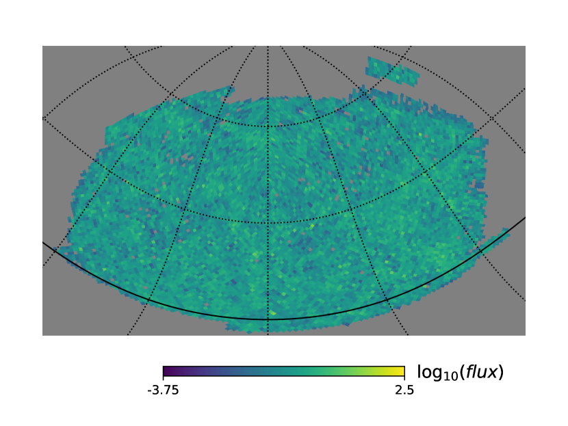
(a) $n=0$

(b) $n=2$

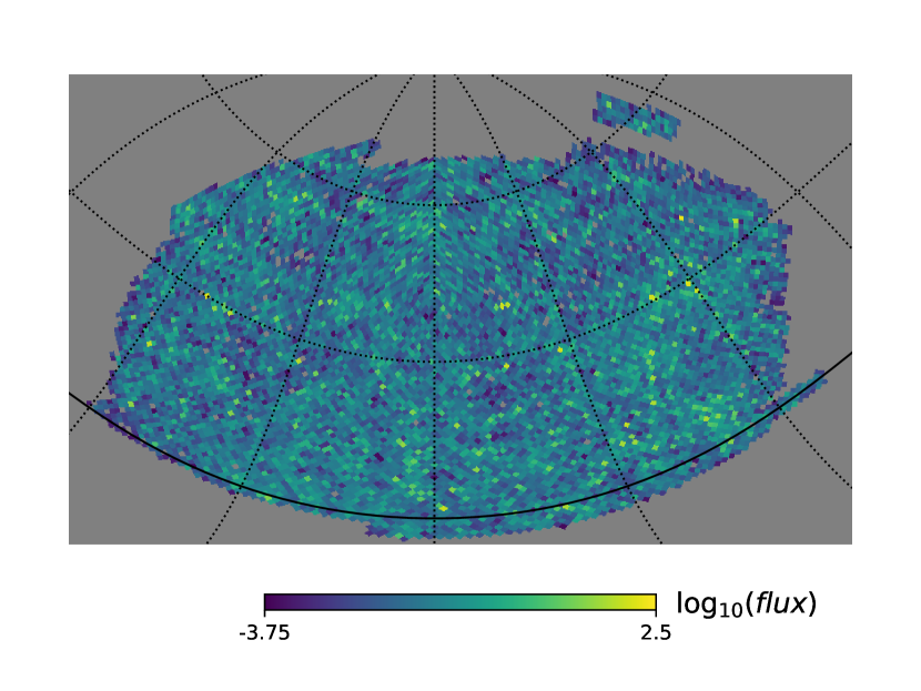
(c) $n=4$

(d) anisotropic background.

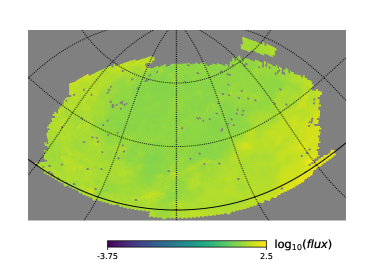
(e) Galactic background.

Figure 2: The flux map models used in our analysis. Panels (a)–(c) represent the dark matter signal model with different values of the velocity-dependence parameter, $n$. Panel (d) represents our toy model for the non-dark matter emission from extragalactic halos, while panel (e) represents the galactic background model. Flux values are in units of photons per pixel, assuming our nominal exposure of $10^{4}~{}{\rm cm}^{2}~{}{\rm yr}$ and a pixel size corresponding to a Healpix resolution of $N_{\rm side}=64$.

For illustration, we present the dark matter annihilation flux maps for $n=0$, $n=2$ and $n=4$ in Figures 2(a), 2(b), and 2(c), respectively. In each case, we show signal only, and normalize the total expected number of photons from dark matter annihilation in extragalactic halos to $5000$, which, given an exposure of $10^{4}~{}{\rm cm}^{2}~{}{\rm yr}$, would be about the largest number of photons consistent with bounds from searches of dSphs, in the case of $p$-wave annihilation. Note that for $n=0$, such a large photon count from extragalactic halos would be inconsistent with bounds from observations of dSphs unless the extragalactic halos had a sizeable boost factor. Similarly, we note that for $n=4$, models consistent with searches of dSphs could produce many more than $5000$ photons in extragalactic halos. We plot the extragalactic anisotropic background flux map in Figure 2(d), assuming the total expected number of photons is 5000, equal to the assumed signal for an exposure of $10^{4}~{}{\rm cm}^{2}~{}{\rm yr}$. We plot the galactic anisotropic background flux map in the energy range $1-100~{}{\rm GeV}$ in Figure 2(e), normalized to the expected number of counts per pixel for the same exposure.

With the mock data generated, we now compute the likelihood of data as a function of our model parameters. We can completely describe the model for the photon probability distribution with the parameters $n$, $N_{{\rm DM}}=\sum_{i}N_{{\rm DM}(n);i}$, $N_{{\rm aniso}}=\sum_{i}N_{{\rm aniso};i}$ and $N_{\rm iso}=N_{{\rm pix}}N_{{\rm iso};i}$. The likelihood for the observed data is given by a product of Poisson likelihood across all pixels:

$$\mathcal{L}(\{d_{0},d_{1},\ldots,d_{N_{\rm pix}}\}|\vec{\theta})=\prod_{i}^{N_{\rm pix}}\frac{N_{i}^{d_{i}}e^{-N_{i}}}{d_{i}!},$$ (4.5)

where $d_{i}$ is the number of photons observed in the $i$th pixel and $\vec{\theta}=(n,N_{\rm DM},N_{\rm aniso},N_{\rm iso})$ is the set of model parameters. The likelihood will provide a way to measure the signal amplitude, $N_{\rm DM}$, in the mock data, as well as a way to distinguish between different values of $n$. In writing Eq. 4.5, we have ignored the impact of the limited resolution of the telescope, which will induce a correlation between neighboring pixels; this approximation is justified for the reasons discussed above. We assume uniform priors on all of the model parameters, so the posterior on these parameters is proportional to the likelihood.

5 Results

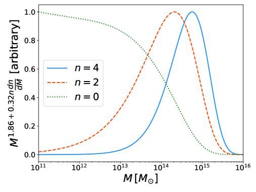
Figure 3: Relative contributions to the annihilation luminosity as a function of halo mass for different models of the annihilation velocity dependence. The annihilation luminosity is expected to scale as $M^{0.86+0.32n}$, where $M$ is the halo mass. The $y$-axis thus represents the contribution to the luminosity per logarithmic interval of mass, normalized to unity. The calculation is performed at $z=0$ and assumes the halo mass function ($dn/dM$) from Ref. [10].

5.1 Halo mass dependence

Before analyzing the mock data described above, we first compute the relative contributions of different halo masses to the expected extragalactic annihilation signal. We assume a flat $\Lambda$CDM cosmological model with parameters matching those preferred by Planck [60]. To describe the abundance of dark matter halos as a function of mass and redshift, we adopt the halo mass function from Ref. [10]. Using our expression Eq. 3.10 for the $J$-factor, we plot the relative contributions to the annihilation signal from logarithmic halo mass bins at $z=0$ in Figure 3.

Consistent with the expectations discussed previously, as $n$ is increased, the halo mass range contributing to the total annihilation luminosity shifts towards higher masses. For the models that we focus on in this analysis ($n=2$ and $n=4$), most of the annihilation luminosity comes from halos above the group scale ($M\sim 10^{13}M_{\odot}$). As noted previously, the catalog described in §2 therefore captures most of the annihilation signal relevant for the models of interest.

5.2 Mock analysis

Having drawn mock data assuming a true model of $p$-wave annihilation ($n=2$) and an exposure of $10^{4}~{}{\rm cm}^{2}~{}{\rm yr}$, we compute the likelihood of the data across a grid of parameter values, assuming either the $n=2$ or the $n=4$ model; we will use these grids to plot marginalized posteriors. Additionally, we use the Nelder-Mead algorithm to maximize the likelihood and determine the best-fit model parameters.

We plot marginalized parameter constraints, assuming the correct model ($n=2$), in Figure 4(a), and assuming the incorrect model ($n=4$) in Figure 4(b). In both figures, the true model is denoted with black crosses and the model which maximizes the likelihood is denoted with red crosses, and we take the exposure to be $10^{4}~{}{\rm cm}^{2}~{}{\rm yr}$, corresponding roughly to the current exposure with Fermi. As discussed above, we have assumed that astrophysical backgrounds associated with extragalactic halos have been cleaned to a level comparable to the dark matter signal. Making these assumptions, it is clear that with the current Fermi exposure, $N_{\rm DM}=0$ is excluded at high significance, meaning that one can easily reject the null hypothesis of no dark matter contribution ($\Delta\ln\mathcal{L}=24.0$). As expected, we do well at reconstructing the parameters when we assume the correct model. In particular, this indicates that the $\sim 10^{4}$ photons one would observe contain enough information to provide very strong evidence for dark matter annihilation, even allowing for a floating background which is correlated with halo mass and an isotropic background of unknown amplitude. But if we assume an incorrect velocity-dependence for the dark matter annihilation cross section, the best-fit point is quite far from the true model, though interestingly, an astrophysics-only explanation (i.e. $N_{\rm DM}=0$) would still be somewhat disfavored.

The difference between the maximum log-likelihoods for the $n=2$ and $n=4$ analyses, $\Delta\ln\mathcal{L}$, and corresponding best-fit parameter values are reported in Table 1. For an exposure comparable to Fermi, we find that the difference in maximum likelihoods is too small to distinguish between the $n=2$ and $n=4$ models at high significance ($\Delta\ln\mathcal{L}=1.1$).

Exposure $=10^{4}\,{\rm cm}^{2}~{}{\rm yr}$	$n=2$ model	$n=4$ model	No DM
$\Delta\ln\mathcal{L}$	0	1.1	24.0
$N_{\rm DM}$ at maximum likelihood	4654.6	1138.1	0
$N_{\rm aniso}$ at maximum likelihood	5536.8	10179.8	13578.7
$N_{\rm iso}$ at maximum likelihood	363835.6	362714.0	360469.3

Table 1: Results of likelihood analyses when the true model is $n=2$. The reported $\Delta\ln\mathcal{L}$ values are measured with respect to the $n=2$ analysis. We assume an exposure of $10^{4}~{}{\rm cm}^{2}~{}{\rm yr}$ and the true parameter values are $N_{\rm DM}=5000$, $N_{\rm aniso}=5000$, and $N_{\rm iso}=363550$.

We then perform a similar analysis, drawing mock data assuming a true model with $n=2$, but with an exposure $10\times$ larger ($10^{5}~{}{\rm cm}^{2}~{}{\rm yr}$). We present the resulting $\Delta\ln\mathcal{L}$ and best-fit normalization parameters in Table 2. With a factor 10 larger exposure, one can clearly distinguish the true velocity-dependence model: $\Delta\ln\mathcal{L}=22.5$. We plot parameter constraints, assuming the correct model ($n=2$), in Figure 5(a), and assuming the incorrect model ($n=4$) in Figure 5(b). In both figures, the true model is denoted with black crosses and the model which maximizes the likelihood is denoted with red crosses, and we take the exposure to be $10^{5}~{}{\rm cm}^{2}~{}{\rm yr}$. Again, the true parameters are recovered to within the uncertainties when analyzing the data with the correct model.

Obtaining an exposure roughly ten times larger than the current Fermi LAT exposure with the same instrument is unlikely. Therefore, it seems that a new telescope (likely a larger instrument, or multiple instruments) will be needed to obtain the photon statistics necessary to distinguish between the $n=2$ and $n=4$ models in the manner we have considered above. To investigate the required properties of such a telescope, we repeat our analysis across a grid of exposure values to build an interpolating function between exposure and $\Delta\ln\mathcal{L}$. A reasonable threshold for rejecting one value of $n$ over another is $\Delta\ln\mathcal{L}\sim 10$. For instance, if the models are compared using the Akaike information criterion [61], this would mean that one model is $\exp(10/2)\approx 150$ times more likely to minimize the information lost by using that model to represent the data. We find that achieving $\Delta\ln\mathcal{L}=10$ would require an exposure 5.4 times larger than Fermi LAT.

Exposure $=10^{5}\,{\rm cm}^{2}~{}{\rm yr}$	$n=2$ model	$n=4$ model	No DM
$\Delta\ln\mathcal{L}$	0	22.5	284.3
$N_{\rm DM}$ at maximum likelihood	50845.9	12189.4	0
$N_{\rm aniso}$ at maximum likelihood	48606.7	99868.2	136061.5
$N_{\rm iso}$ at maximum likelihood	3635062.4	3622512.9	3598680.5

Table 2: Same as Table 1, but with $10\times$ larger exposure. The larger exposure means the true parameter values are now $N_{\rm DM}=50000$, $N_{\rm aniso}=50000$, and $N_{\rm iso}=3635497$.

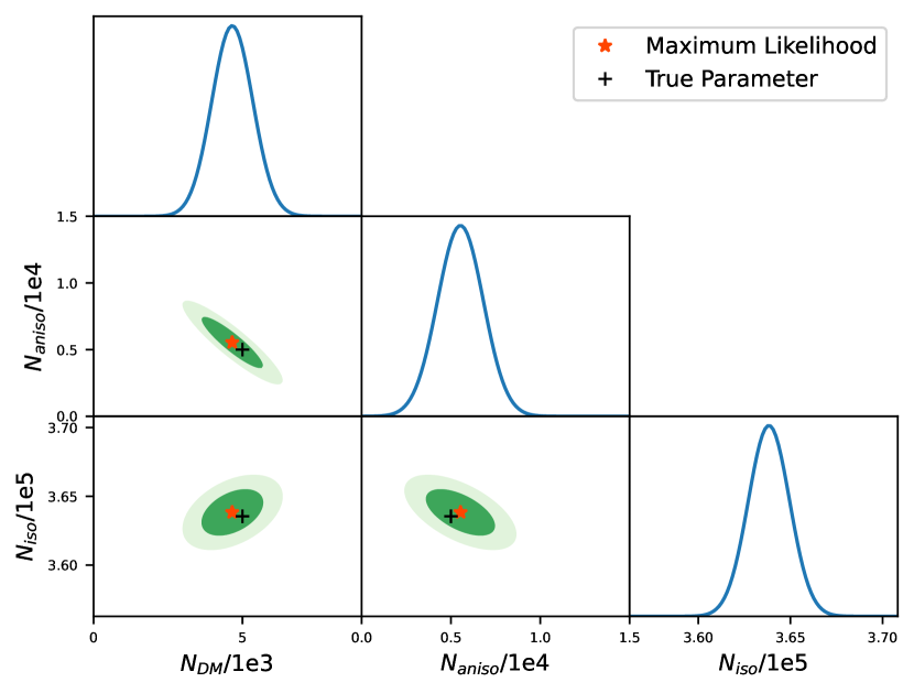
(a) Data: $n=2$, Model: $n=2$.

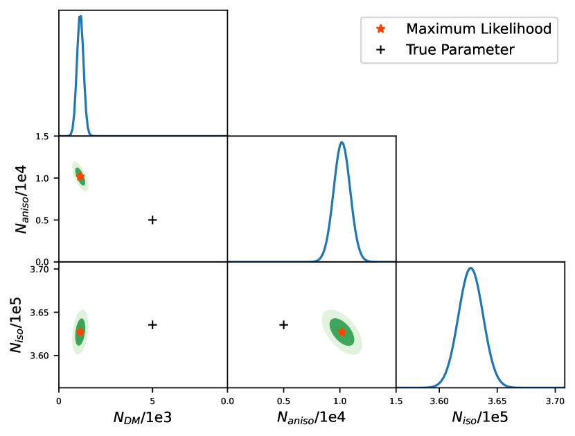
(b) Data: $n=2$, Model: $n=4$.

Figure 4: Results of the likelihood analysis of mock gamma-ray data. The top panel (a) shows the results of analyzing mock data generated assuming $n=2$ with the correct velocity-dependence model; bottom panel (b) shows the results of analyzing the same mock data with a different, $n=4$, velocity-dependence model. We assume an exposure of $10^{4}~{}{\rm cm}^{2}~{}{\rm yr}$, roughly equal to the current exposure of Fermi. Contours indicate the 68% (dark green) and 95% (light green) credible intervals on the model parameters. Red cross hairs represent the location of the maximum likelihood (see Table 1). Black cross hairs indicate the normalization of the true model: [$N_{\rm DM}$, $N_{\rm aniso}$, $N_{\rm iso}$] = [5000, 5000, $363550$].

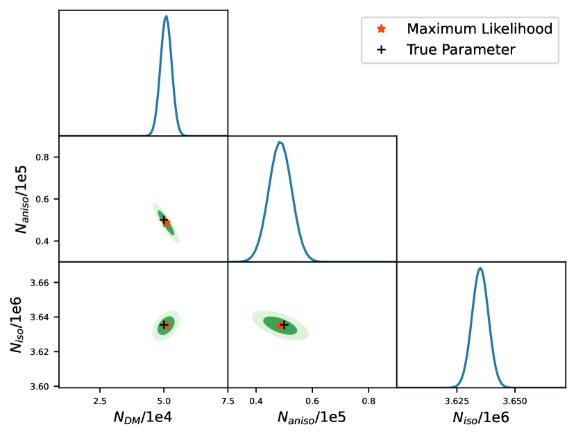
(a) Data: $n=2$, Model: $n=2$.

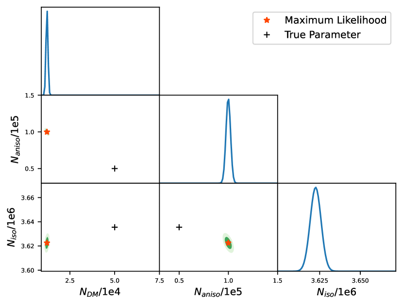
(b) Data: $n=2$, Model: $n=4$

Figure 5: Same as Fig. 4, but for an exposure of $10^{5}~{}{\rm cm}^{2}~{}{\rm yr}$, which is roughly $10\times$ larger than currently achieved by Fermi. Red cross hairs represent the location of the maximum likelihood (see Table 2). Black cross hairs indicate the normalization of the true model: [$N_{\rm DM}$, $N_{\rm aniso}$, $N_{\rm iso}$] = [50000, 50000, $3635497$]. In some cases, the contours are so small that they are not visible below the markers.

6 Conclusion

We have considered the indirect detection of velocity-dependent dark matter annihilation in extragalactic halos using gamma-ray signals. Extragalactic halos are an especially interesting target because, of all bound astrophysical objects, they have among the largest particle velocities. Thus, if $\sigma v\propto(v/c)^{n}$ for $n>0$, one expects the dark matter annihilation signal from extragalactic halos to be enhanced relative to other commonly-studied targets, such as galactic subhalos, dwarf spheroidal galaxies, and the Galactic Center.

Our analysis makes several optimistic assumptions, including that backgrounds are modelled perfectly. In particular, although we incorporate anisotropic astrophysical backgrounds which are correlated with the halo map (arising from astrophysical processes in galaxies), we assume that the dependence of the astrophysical background flux on the halo mass is a simple proportionality, which can thus be distinguished from the dark matter annihilation signal.

Even with these optimistic assumptions, we find that there is not enough information in current Fermi data to detect photons produced by $s$-wave dark matter annihilation in the extragalactic halos in our catalog, assuming $\Phi_{PP}$ is set by current limits from dSphs. Our analysis assumes no boost to the dark matter signal arising from the presence of subhalos within the main halos. In the absence of a large boost factor, any model which could be observed in searches of extragalactic halos would already be ruled out by searches of dSphs.

For the case of $p$-wave annihilation, although the current Fermi data contains enough information to reject the null hypothesis of no dark matter contribution, it only marginally favors the true model of annihilation over an allowed alternative model, such as $d$-wave annihilation. But a factor of 10 larger exposure would allow one to distinguish the correct model of dark matter annihilation from the incorrect one with high significance.

Perhaps the most important avenue for future work is in the characterization of astrophysical backgrounds, particular those which could be correlated with the dark matter signal. One might hope that future developments in multi-wavelength astronomy would allow one to correlate a gamma-ray signal from astrophysical processes in a halo with emission in other bands, resulting in a more accurate extragalactic anisotropic background map.

Acknowledgements

JK is supported in part by DOE grant DE-SC0010504. JR is supported by NSF grant AST-1934744. We thank an anonymous referee for comments on our manuscript.

References

- Abdo et al. [2010] A. A. Abdo et al. Observations of Milky Way Dwarf Spheroidal galaxies with the Fermi-LAT detector and constraints on Dark Matter models. Astrophys. J., 712:147–158, 2010. doi: 10.1088/0004-637X/712/1/147.
- Ackermann et al. [2011] M. Ackermann et al. Constraining Dark Matter Models from a Combined Analysis of Milky Way Satellites with the Fermi Large Area Telescope. Phys. Rev. Lett., 107:241302, 2011. doi: 10.1103/PhysRevLett.107.241302.
- Ackermann et al. [2014] M. Ackermann et al. Dark Matter Constraints from Observations of 25 Milky Way Satellite Galaxies with the Fermi Large Area Telescope. Phys. Rev. D, 89:042001, 2014. doi: 10.1103/PhysRevD.89.042001.
- Ackermann et al. [2015] M. Ackermann et al. Searching for Dark Matter Annihilation from Milky Way Dwarf Spheroidal Galaxies with Six Years of Fermi Large Area Telescope Data. Phys. Rev. Lett., 115(23):231301, 2015. doi: 10.1103/PhysRevLett.115.231301.
- Goodenough and Hooper [2009] Lisa Goodenough and Dan Hooper. Possible Evidence For Dark Matter Annihilation In The Inner Milky Way From The Fermi Gamma Ray Space Telescope. arXiv e-prints, art. arXiv:0910.2998, October 2009.
- Hooper and Goodenough [2011] Dan Hooper and Lisa Goodenough. Dark Matter Annihilation in The Galactic Center As Seen by the Fermi Gamma Ray Space Telescope. Phys. Lett. B, 697:412–428, 2011. doi: 10.1016/j.physletb.2011.02.029.
- Abazajian and Kaplinghat [2012] Kevork N. Abazajian and Manoj Kaplinghat. Detection of a Gamma-Ray Source in the Galactic Center Consistent with Extended Emission from Dark Matter Annihilation and Concentrated Astrophysical Emission. Phys. Rev. D, 86:083511, 2012. doi: 10.1103/PhysRevD.86.083511. [Erratum: Phys.Rev.D 87, 129902 (2013)].
- Daylan et al. [2016] Tansu Daylan, Douglas P. Finkbeiner, Dan Hooper, Tim Linden, Stephen K. N. Portillo, Nicholas L. Rodd, and Tracy R. Slatyer. The characterization of the gamma-ray signal from the central Milky Way: A case for annihilating dark matter. Phys. Dark Univ., 12:1–23, 2016. doi: 10.1016/j.dark.2015.12.005.
- Ackermann et al. [2017] M. Ackermann et al. The Fermi Galactic Center GeV Excess and Implications for Dark Matter. Astrophys. J., 840(1):43, 2017. doi: 10.3847/1538-4357/aa6cab.
- Tinker et al. [2008] Jeremy Tinker, Andrey V. Kravtsov, Anatoly Klypin, Kevork Abazajian, Michael Warren, Gustavo Yepes, Stefan Gottlöber, and Daniel E. Holz. Toward a Halo Mass Function for Precision Cosmology: The Limits of Universality. ApJ, 688(2):709–728, December 2008. doi: 10.1086/591439.
- Regis et al. [2015] Marco Regis, Jun-Qing Xia, Alessandro Cuoco, Enzo Branchini, Nicolao Fornengo, and Matteo Viel. Particle dark matter searches outside the Local Group. Phys. Rev. Lett., 114(24):241301, 2015. doi: 10.1103/PhysRevLett.114.241301.
- Stecker and Venters [2011] Floyd W. Stecker and Tonia M. Venters. Components of the Extragalactic Gamma-ray Background. ApJ, 736(1):40, July 2011. doi: 10.1088/0004-637X/736/1/40.
- Sánchez-Conde et al. [2011] Miguel A. Sánchez-Conde, Mirco Cannoni, Fabio Zandanel, Mario E. Gómez, and Francisco Prada. Dark matter searches with Cherenkov telescopes: nearby dwarf galaxies or local galaxy clusters? JCAP, 2011(12):011, December 2011. doi: 10.1088/1475-7516/2011/12/011.
- Nezri et al. [2012] E. Nezri, R. White, C. Combet, J. A. Hinton, D. Maurin, and E. Pointecouteau. -rays from annihilating dark matter in galaxy clusters: stacking versus single source analysis. MNRAS, 425(1):477–489, September 2012. doi: 10.1111/j.1365-2966.2012.21484.x.
- Jeltema et al. [2009] Tesla E. Jeltema, John Kehayias, and Stefano Profumo. Gamma rays from clusters and groups of galaxies: Cosmic rays versus dark matter. Phys. Rev. D, 80(2):023005, July 2009. doi: 10.1103/PhysRevD.80.023005.
- Piccirillo et al. [2022] Erin Piccirillo, Keagan Blanchette, Nassim Bozorgnia, Louis E. Strigari, Carlos S. Frenk, Robert J. J. Grand, and Federico Marinacci. Velocity-dependent annihilation radiation from dark matter subhalos in cosmological simulations. arXiv e-prints, art. arXiv:2203.08853, March 2022.
- Lacroix et al. [2022] Thomas Lacroix, Gaétan Facchinetti, Judit Pérez-Romero, Martin Stref, Julien Lavalle, David Maurin, and Miguel A. Sánchez-Conde. Classification of gamma-ray targets for velocity-dependent and subhalo-boosted dark-matter annihilation. arXiv e-prints, art. arXiv:2203.16440, March 2022.
- Chang et al. [2018] Laura J. Chang, Mariangela Lisanti, and Siddharth Mishra-Sharma. Search for dark matter annihilation in the Milky Way halo. Phys. Rev. D, 98(12):123004, 2018. doi: 10.1103/PhysRevD.98.123004.
- Hooper et al. [2020] Dan Hooper, Rebecca K. Leane, Yu-Dai Tsai, Shalma Wegsman, and Samuel J. Witte. A systematic study of hidden sector dark matter:application to the gamma-ray and antiproton excesses. JHEP, 07(07):163, 2020. doi: 10.1007/JHEP07(2020)163.
- Boddy et al. [2018a] Kimberly K. Boddy, Jason Kumar, and Louis E. Strigari. Effective J -factor of the Galactic Center for velocity-dependent dark matter annihilation. Phys. Rev. D, 98(6):063012, 2018a. doi: 10.1103/PhysRevD.98.063012.
- Lim et al. [2017] S. H. Lim, H. J. Mo, Yi Lu, Huiyuan Wang, and Xiaohu Yang. Galaxy groups in the low-redshift Universe. MNRAS, 470(3):2982–3005, September 2017. doi: 10.1093/mnras/stx1462.
- Yang et al. [2005] Xiaohu Yang, H. J. Mo, Frank C. van den Bosch, and Y. P. Jing. A halo-based galaxy group finder: calibration and application to the 2dFGRS. MNRAS, 356(4):1293–1307, February 2005. doi: 10.1111/j.1365-2966.2005.08560.x.
- Yang et al. [2007] Xiaohu Yang, H. J. Mo, Frank C. van den Bosch, Anna Pasquali, Cheng Li, and Marco Barden. Galaxy Groups in the SDSS DR4. I. The Catalog and Basic Properties. ApJ, 671(1):153–170, December 2007. doi: 10.1086/522027.
- Navarro et al. [1997] Julio F. Navarro, Carlos S. Frenk, and Simon D. M. White. A Universal Density Profile from Hierarchical Clustering. ApJ, 490(2):493–508, December 1997. doi: 10.1086/304888.
- Bennett et al. [2013] C. L. Bennett, D. Larson, J. L. Weiland, N. Jarosik, G. Hinshaw, N. Odegard, K. M. Smith, R. S. Hill, B. Gold, M. Halpern, E. Komatsu, M. R. Nolta, L. Page, D. N. Spergel, E. Wollack, J. Dunkley, A. Kogut, M. Limon, S. S. Meyer, G. S. Tucker, and E. L. Wright. Nine-year Wilkinson Microwave Anisotropy Probe (WMAP) Observations: Final Maps and Results. ApJS, 208(2):20, October 2013. doi: 10.1088/0067-0049/208/2/20.
- Boddy et al. [2017] Kimberly K. Boddy, Jason Kumar, Louis E. Strigari, and Mei-Yu Wang. Sommerfeld-Enhanced -Factors For Dwarf Spheroidal Galaxies. Phys. Rev. D, 95(12):123008, 2017. doi: 10.1103/PhysRevD.95.123008.
- Jing and Suto [2002] Y. P. Jing and Yasushi Suto. Triaxial Modeling of Halo Density Profiles with High-Resolution N-Body Simulations. ApJ, 574(2):538–553, August 2002. doi: 10.1086/341065.
- Ullio et al. [2001] Piero Ullio, Hongsheng Zhao, and Marc Kamionkowski. Dark-matter spike at the galactic center? Phys. Rev. D, 64(4):043504, August 2001. doi: 10.1103/PhysRevD.64.043504.
- Amin and Wizansky [2008] Mustafa A. Amin and Tommer Wizansky. Relativistic dark matter at the galactic center. Phys. Rev. D, 77(12):123510, June 2008. doi: 10.1103/PhysRevD.77.123510.
- Sandick et al. [2018] Pearl Sandick, Kuver Sinha, and Takahiro Yamamoto. Black Holes, Dark Matter Spikes, and Constraints on Simplified Models with -Channel Mediators. Phys. Rev. D, 98(3):035004, 2018. doi: 10.1103/PhysRevD.98.035004.
- Kumar and Marfatia [2013] Jason Kumar and Danny Marfatia. Matrix element analyses of dark matter scattering and annihilation. Phys. Rev. D, 88(1):014035, 2013. doi: 10.1103/PhysRevD.88.014035.
- Giacchino et al. [2013] Federica Giacchino, Laura Lopez-Honorez, and Michel H. G. Tytgat. Scalar Dark Matter Models with Significant Internal Bremsstrahlung. JCAP, 10:025, 2013. doi: 10.1088/1475-7516/2013/10/025.
- Toma [2013] Takashi Toma. Internal Bremsstrahlung Signature of Real Scalar Dark Matter and Consistency with Thermal Relic Density. Phys. Rev. Lett., 111:091301, 2013. doi: 10.1103/PhysRevLett.111.091301.
- Kopp et al. [2016] Joachim Kopp, Jia Liu, Tracy R. Slatyer, Xiao-Ping Wang, and Wei Xue. Impeded dark matter. Journal of High Energy Physics, 2016(12), dec 2016. doi: 10.1007/jhep12(2016)033. URL https://doi.org/10.1007%2Fjhep12%282016%29033.
- Boddy et al. [2019] Kimberly K. Boddy, Jason Kumar, Jack Runburg, and Louis E. Strigari. Angular distribution of gamma-ray emission from velocity-dependent dark matter annihilation in subhalos. Phys. Rev. D, 100(6):063019, 2019. doi: 10.1103/PhysRevD.100.063019.
- Robertson and Zentner [2009] Brant E. Robertson and Andrew R. Zentner. Dark matter annihilation rates with velocity-dependent annihilation cross sections. Phys. Rev. D, 79:083525, Apr 2009. doi: 10.1103/PhysRevD.79.083525.
- Belotsky et al. [2014] K. Belotsky, A. Kirillov, and M. Khlopov. Gamma-ray evidence for dark matter clumps. Gravitation and Cosmology, 20(1):47–54, jan 2014. doi: 10.1134/s0202289314010022.
- Ferrer and Hunter [2013] Francesc Ferrer and Daniel R Hunter. The impact of the phase-space density on the indirect detection of dark matter. Journal of Cosmology and Astroparticle Physics, 2013(09):005–005, sep 2013. doi: 10.1088/1475-7516/2013/09/005.
- Zhao et al. [2018] Yi Zhao, Xiao-Jun Bi, Peng-Fei Yin, and Xinmin Zhang. Constraint on the velocity dependent dark matter annihilation cross section from gamma-ray and kinematic observations of ultrafaint dwarf galaxies. Phys. Rev. D, 97:063013, Mar 2018. doi: 10.1103/PhysRevD.97.063013.
- Petač et al. [2018] Mihael Petač, Piero Ullio, and Mauro Valli. On velocity-dependent dark matter annihilations in dwarf satellites. Journal of Cosmology and Astroparticle Physics, 2018(12):039–039, dec 2018. doi: 10.1088/1475-7516/2018/12/039.
- Lacroix et al. [2018] Thomas Lacroix, Martin Stref, and Julien Lavalle. Anatomy of eddington-like inversion methods in the context of dark matter searches. Journal of Cosmology and Astroparticle Physics, 2018(09):040–040, sep 2018. doi: 10.1088/1475-7516/2018/09/040.
- Boddy et al. [2020] Kimberly K. Boddy, Jason Kumar, Andrew B. Pace, Jack Runburg, and Louis E. Strigari. Effective -factors for Milky Way dwarf spheroidal galaxies with velocity-dependent annihilation. Phys. Rev. D, 102(2):023029, 2020. doi: 10.1103/PhysRevD.102.023029.
- Boucher et al. [2021] Bradly Boucher, Jason Kumar, Van B. Le, and Jack Runburg. -factors for Velocity-dependent Dark Matter. arXiv e-prints, art. arXiv:2110.09653, October 2021.
- Duffy et al. [2008] Alan R. Duffy, Joop Schaye, Scott T. Kay, and Claudio Dalla Vecchia. Dark matter halo concentrations in the Wilkinson Microwave Anisotropy Probe year 5 cosmology. MNRAS, 390(1):L64–L68, October 2008. doi: 10.1111/j.1745-3933.2008.00537.x.
- Diemer and Kravtsov [2015] Benedikt Diemer and Andrey V. Kravtsov. A Universal Model for Halo Concentrations. ApJ, 799(1):108, January 2015. doi: 10.1088/0004-637X/799/1/108.
- Diemer [2018] Benedikt Diemer. COLOSSUS: A Python Toolkit for Cosmology, Large-scale Structure, and Dark Matter Halos. ApJS, 239(2):35, December 2018. doi: 10.3847/1538-4365/aaee8c.
- Zhao et al. [2003] D. H. Zhao, Y. P. Jing, H. J. Mo, and G. Börner. Mass and Redshift Dependence of Dark Halo Structure. ApJ, 597(1):L9–L12, November 2003. doi: 10.1086/379734.
- Zahid et al. [2018] H. Jabran Zahid, Jubee Sohn, and Margaret J. Geller. Stellar Velocity Dispersion: Linking Quiescent Galaxies to Their Dark Matter Halos. The Astrophysical Journal, 859(2):96, May 2018. ISSN 1538-4357. doi: 10.3847/1538-4357/aabe31.
- Diemand and Moore [2011] Jürg Diemand and Ben Moore. The Structure and Evolution of Cold Dark Matter Halos. Advanced Science Letters, 4(2):297–310, February 2011. doi: 10.1166/asl.2011.1211.
- Salucci [2019] Paolo Salucci. The distribution of dark matter in galaxies. A&A Rev., 27(1):2, February 2019. doi: 10.1007/s00159-018-0113-1.
- Sánchez-Conde and Prada [2014] Miguel A. Sánchez-Conde and Francisco Prada. The flattening of the concentration–mass relation towards low halo masses and its implications for the annihilation signal boost. Mon. Not. Roy. Astron. Soc., 442(3):2271–2277, 2014. doi: 10.1093/mnras/stu1014.
- Giocoli et al. [2010] Carlo Giocoli, Giuseppe Tormen, Ravi K. Sheth, and Frank C. van den Bosch. The substructure hierarchy in dark matter haloes. MNRAS, 404(1):502–517, May 2010. doi: 10.1111/j.1365-2966.2010.16311.x.
- Inoue et al. [2005] Susumu Inoue, Felix A. Aharonian, and Naoshi Sugiyama. Hard X-Ray and Gamma-Ray Emission Induced by Ultra-High-Energy Protons in Cluster Accretion Shocks. ApJ, 628(1):L9–L12, July 2005. doi: 10.1086/432602.
- Kornecki et al. [2020] P. Kornecki, L. J. Pellizza, S. del Palacio, A. L. Müller, J. F. Albacete-Colombo, and G. E. Romero. -ray/infrared luminosity correlation of star-forming galaxies. A&A, 641:A147, September 2020. doi: 10.1051/0004-6361/202038428.
- Abdollahi et al. [2020] S. Abdollahi et al. Fermi large area telescope fourth source catalog. The Astrophysical Journal Supplement Series, 247(1):33, Mar 2020. ISSN 1538-4365. doi: 10.3847/1538-4365/ab6bcb.
- Lacroix et al. [2022] Thomas Lacroix, Gaétan Facchinetti, Judit Pérez-Romero, Martin Stref, Julien Lavalle, David Maurin, and Miguel A. Sánchez-Conde. Classification of gamma-ray targets for velocity-dependent and subhalo-boosted dark-matter annihilation. 3 2022.
- Geringer-Sameth and Koushiappas [2011] Alex Geringer-Sameth and Savvas M. Koushiappas. Exclusion of canonical WIMPs by the joint analysis of Milky Way dwarfs with Fermi. Phys. Rev. Lett., 107:241303, 2011. doi: 10.1103/PhysRevLett.107.241303.
- Boddy et al. [2018b] Kimberly Boddy, Jason Kumar, Danny Marfatia, and Pearl Sandick. Model-independent constraints on dark matter annihilation in dwarf spheroidal galaxies. Phys. Rev. D, 97(9):095031, 2018b. doi: 10.1103/PhysRevD.97.095031.
- Boddy et al. [2021] Kimberly K. Boddy, Stephen Hill, Jason Kumar, Pearl Sandick, and Barmak Shams Es Haghi. MADHAT: Model-Agnostic Dark Halo Analysis Tool. Comput. Phys. Commun., 261:107815, 2021. doi: 10.1016/j.cpc.2020.107815.
- Planck Collaboration et al. [2020] Planck Collaboration et al. Planck 2018 results. VI. Cosmological parameters. A&A, 641:A6, September 2020. doi: 10.1051/0004-6361/201833910.
- Hastie et al. [2001] Trevor Hastie, Robert Tibshirani, and Jerome Friedman. The Elements of Statistical Learning. Springer Series in Statistics. Springer New York Inc., New York, NY, USA, 2001.