Topological Langmuir-cyclotron wave

Abstract

A theoretical framework is developed to describe the Topological Langmuir-Cyclotron Wave (TLCW), a recently identified topological surface excitation in magnetized plasmas. As a topological wave, the TLCW propagates unidirectionally without scattering in complex boundaries. The TLCW is studied theoretically as a spectral flow of the Hamiltonian Pseudo-Differential-Operator (PDO) $\hat{H}$ for waves in an inhomogeneous plasma. The semi-classical parameter of the Weyl quantization for plasma waves is identified to be the ratio between electron gyro-radius and the inhomogeneity scale length of the system. Hermitian eigenmode bundles of the bulk Hamiltonian symbol $H$ for plasma waves are formally defined. Because momentum space in classical continuous media is contractible in general, the topology of the eigenmode bundles over momentum space is trivial. This is in stark contrast to condensed matters. Nontrivial topology of the eigenmode bundles in classical continuous media only exists over phase space. A boundary isomorphism theorem is established to facilitate the calculation of Chern numbers of eigenmode bundles over non-contractible manifolds in phase space. It also defines a topological charge of an isolated Weyl point in phase space without adopting any connection. Using these algebraic topological techniques and an index theorem formulated by Faure, it is rigorously proven that the nontrivial topology at the Weyl point of the Langmuir wave-cyclotron wave resonance generates the TLCW as a spectral flow. It is shown that the TLCW can be faithfully modeled by a tilted Dirac cone in phase space. An analytical solution of the entire spectrum of the PDO of a generic tilted phase space Dirac cone, including its spectral flow, is given. The spectral flow index of a tilted Dirac cone is one, and its mode structure is a shifted Gaussian function.

I Introduction

Topological wave in classical continuous media is an active research topic for its practical importance. For example, it was discovered [1, 2] that the well-known equatorial Kelvin wave, which can trigger an El Nino episode [3], is a topological wave in nature. Topological waves in cold magnetized plasmas have been recently studied [4, 5]. Through comprehensive numerical simulations and heuristic application of the principle of bulk-edge correspondence, a topological surface excitation called Topological Langmuir-Cyclotron Wave (TLCW) was identified [5, 6]. As a topological wave, the TLCW has topological robustness, i.e., it is unidirectional and free of scattering and reflection. Thus, the TLCW excitation is expected to be experimentally observable.

In the present study, we develop a theoretical framework to describe the TLCW and rigorously prove that it is produced by the nontrivial topology at the Weyl point due to the Langmuir wave-cyclotron wave resonance using an index theorem for spectral flows formulated by Faure [2] and tools of algebraic topology. Most of the techniques developed are applicable to general topological waves in classical continuous media as well. The key developments of the present study are summarized as follows.

1. The TLCW is theoretically described as a spectral flow of the global Hamiltonian Pseudo-Differential-Operator (PDO) $\hat{H}$ for waves in an inhomogeneous magnetized plasma. For this problem, the semi-classical parameter of the Weyl quantization operator, which maps the bulk Hamiltonian symbol $H$ to $\hat{H}$, is identified as the ratio between electron gyro-radius and the scale length of the inhomogeneity. We emphasize the important role of the semi-classical parameters and the necessity to identify them for topological waves in classical continuous media according to the nature of the physics under investigation.

2. We formally construct the Hermitian eigenmode bundles of the bulk Hamiltonian symbol $H$, and show that it is the topology of the eigenmode bundles over non-contractible manifolds in phase space that determines the properties of spectral flows for classical continuous media. We show that the topology of eigenmode bundles on momentum (wavenumber) space is trivial in classical continuous media, unlike in condensed matters. Without modification, the Atiyah-Patodi-Singer (APS) index theorem [7] proved for spectral flows over $S^{1}$ is only applicable to condensed matters, and Faure’s index theorem [2] for spectral flows over $\mathbb{R}$-valued wavenumbers should be adopted for classical continuous media.

3. A boundary isomorphism theorem (Theorem 12) is proved to facilitate the calculation of Chern numbers of eigenmode bundles over a 2D sphere in phase space. The theorem also defines a topological charge of an isolated Weyl point in phase space using a topological method, i.e., without using any connection.

4. An analytical solution of the global Hamiltonian PDO of a generic tilted Dirac cone in phase space is found, which generalizes the previous result for a straight Dirac cone [2]. The spectral flow index of a tilted phase space Dirac cone is calculated to be one, and the mode structure of the spectral flow is found to be a shifted Gaussian function.

5. These tools are applied to prove the existence of the TLCW in magnetized plasmas with the spectral flow index being one. The Chern theorem (Theorem 6), instead of the Berry connection or any other connection, was used to calculate the Chern numbers. And it is shown that the TLCW can be faithfully described by a tilted Dirac cone in phase space.

The paper is organized as follows. In Sec. II, we pose the problem to be studied and describe the general properties of the TLCW identified by numerical simulations. Section III presents additional numerical evidence and simulation results of the TLCW. In Sec. IV, we define the Hermitian eigenmode bundles of waves in classical continuous media and develop algebraic topological tools to study the nontrivial topology of eigenmode bundles over phase space. The existence of TLCW as a spectral flow is proven in Sec. V. We construct a tilted Dirac cone model for the TLCW in Sec. VI, and the entire spectrum of the PDO of a generic tilted Dirac cone, including its spectral flow, is solved analytically.

II Problem statement and general properties of TLCW

We first pose the problem to be addressed in the present study, introduce the governing equations, set up the class of equilibrium plasmas that might admit the TLCW, and describe its general properties.

Consider a cold magnetized plasma with fixed ions. The equilibrium magnetic field $\boldsymbol{B}_{0}=B_{0}\boldsymbol{e}_{z}$ is assumed to be constant. Because the plasma is cold, any density profile $n(\boldsymbol{r})$ is an admissible equilibrium. Denote by $L\sim\left|n/\nabla n\right|$ the characteristic scale length of $n$. There is no equilibrium electrical field and electron flow velocity, i.e., $\boldsymbol{v}_{0}=0$ and $\boldsymbol{E}_{0}=0.$ The linear dynamics of the system is described by the following equations for the perturbed electromagnetic field $\boldsymbol{E}$ and $\boldsymbol{B}$, and the perturbed electron flow $\boldsymbol{v}$.

$$\partial_{t}\boldsymbol{v}=-e\boldsymbol{E}/m_{e}-\Omega\boldsymbol{v}\times\boldsymbol{e}_{z},$$ (1)

$$\partial_{t}\boldsymbol{E}=c\nabla\times\boldsymbol{B}+4\pi en\boldsymbol{v},$$ (2)

$$\partial_{t}\boldsymbol{B}=-c\nabla\times\boldsymbol{E},$$ (3)

where $\Omega=eB_{0}/m_{e}c$ is the cyclotron frequency, $m_{\mathrm{e}}$ is the electron mass, and $e>0$ is the elementary charge. We normalize $\boldsymbol{v}$ by $1/\sqrt{4\pi n(\boldsymbol{r})m_{\mathrm{e}}}$, $t$ by $1/\Omega$, $\boldsymbol{r}$ by $L$, and $\nabla$ by $1/L$. In the normalized variables, Eqs. (1)-(3) can be written as

$$\mathrm{i}\partial_{t}\psi =\hat{H}\psi,$$ (4)

$$\psi =\left(\begin{array}[]{c}\boldsymbol{v}\\ \boldsymbol{E}\\ \boldsymbol{B}\end{array}\right),$$ (8)

$$\hat{H} (\boldsymbol{r},-\mathrm{i}\eta\nabla)=\begin{pmatrix}\mathrm{i}\boldsymbol{e}_{z}\times&-\mathrm{i}\omega_{\text{p}}&0\\ \mathrm{i}\omega_{\text{p}}&0&\mathrm{i}\eta\nabla\times\\ 0&-\mathrm{i}\eta\nabla\times&0\end{pmatrix},$$ (9)

where $\mathrm{i}\boldsymbol{e}_{z}\times$ and $\mathrm{i}\eta\nabla\times$ denote $3\times 3$ anti-symmetric matrices corresponding to $\boldsymbol{e}_{z}$ and $\nabla$, respectively. For a generic vector $\boldsymbol{u}=(u_{x},u_{y},u_{z})$ in $\mathbb{R}^{3},$ the corresponding $3\times 3$ anti-symmetric matrix is defined to be

$$\boldsymbol{u}\times\equiv\begin{pmatrix}0&-u_{z}&u_{y}\\ u_{z}&0&-u_{x}\\ -u_{y}&u_{x}&0\end{pmatrix}.$$ (10)

In Eq. (9), $\omega_{\mathrm{p}}(\boldsymbol{r})=\sqrt{4\pi n(\boldsymbol{r})e^{2}/m_{\mathrm{e}}}/\Omega$ is the local plasma frequency normalized by $\Omega,$ and $\eta\equiv c/(L\Omega)\sim\rho_{e}/L$ is a dimensionless parameter proportional to the ratio between electron gyro-radius and the scale length of $n$. Here, $\eta$ is assumed to be small, i.e., $\eta\ll 1$, and it plays the role of the semi-classical parameter for the Weyl quantization of this problem.

The Weyl quantization operator

$$\mathrm{Op}_{\eta}:f\rightarrow\hat{f}=\mathrm{Op}_{\eta}(f)$$ (11)

maps a function in phase space $f(\boldsymbol{r},\boldsymbol{k})$, called a symbol, to an Pseudo-Differential-Operator (PDO) $\hat{f}$ on functions $\psi(\boldsymbol{r})$ on the $n$-dimensional configuration space. The operator $\hat{f}=\mathrm{Op}_{\eta}(f)$ is defined by

$$\hat{f}\psi(\boldsymbol{r})=\frac{1}{(2\pi\eta)^{n}}\int f\left(\frac{\boldsymbol{r}+\boldsymbol{s}}{2},\boldsymbol{k}\right)\exp\left(\frac{\mathrm{i}\boldsymbol{k}\cdot\left(\boldsymbol{x}-\boldsymbol{y}\right)}{\eta}\right)\psi(\boldsymbol{s})\mathrm{d}\boldsymbol{s}\mathrm{d}\boldsymbol{k}\thinspace.$$ (12)

In particular, we have $\hat{\boldsymbol{k}}=-\mathrm{i}\eta\nabla$.

For the $\hat{H}$ given by Eq. (9), its pre-image $H$, i.e., the symbol $H$ satisfying $\hat{H}=\mathrm{Op}_{\eta}(H)$, is

$$H(\boldsymbol{r},\boldsymbol{k})=\begin{pmatrix}\mathrm{i}\boldsymbol{e}_{z}\times&-\mathrm{i}\omega_{\text{p}}&0\\ \mathrm{i}\omega_{\text{p}}&0&-\boldsymbol{k}\times\\ 0&\boldsymbol{k}\times&0\end{pmatrix}.$$ (13)

In quantum theory, the semi-classical parameter is typically the Plank constant $\hbar$, and it is a crucial parameter in the index theorems for spectral flow [7, 2] of PDOs. For the plasma waves in the present study, the semi-classical parameter is identified to be $\eta\equiv c/(L\Omega)$, which is the ratio between electron gyro-radius and the scale length of the equilibrium plasma. Notice that in the PDO $\hat{H}(\boldsymbol{r},-\mathrm{i}\eta\nabla)$ the differential operator $\nabla$ is normalized by $1/L$, but in the symbol $H(\boldsymbol{r},\boldsymbol{k})$ the wavenumber $\boldsymbol{k}$ is normalized by $\Omega/c$, thanks to the small semi-classical parameter $\eta$ strategically placed in the Weyl quantization operator $\mathrm{Op}_{\eta}$. This structure between the PDO and the symbol is required for the application of the index theorem of spectral flow [7, 2]. In the study of other topological properties of classical media, such as electromagnetic materials [8, 9, 10, 11], fluid systems [1, 2, 12, 13, 14, 15, 16, 17, 18, 19], and magnetized plasmas [20, 21, 22, 4, 23, 5, 6, 24, 25], we believe that appropriate semi-classical parameters should also be carefully determined first based on the specific nature of the problems under investigation.

In plasma physics, the symbol $H(\boldsymbol{r},\boldsymbol{k})$ is called the local Hamiltonian of the system, but it is known as the bulk Hamiltonian in condensed matter physics. Thus, in the present context, the phrases “bulk modes” and “local modes” have the same meaning, referring to the spectrum determined by $H(\boldsymbol{r},\boldsymbol{k})$ locally at each $\boldsymbol{r}$ and each $\boldsymbol{k}$ separately. The spectrum of the PDO $\hat{H}(\boldsymbol{r},-\mathrm{i}\eta\nabla)$ will be called global modes. The edge modes, including topological edge modes, refer to the global modes of $\hat{H}(\boldsymbol{r},-\mathrm{i}\eta\nabla)$ whose mode structures are non-vanishing only in some narrow interface regions. It is unfortunate that the phrases “local modes” and “edge modes”, defined in different branches of physics, have very different meanings.

For a fixed $\boldsymbol{r}$ and a fixed $\boldsymbol{k}$, $H(\boldsymbol{r},\boldsymbol{k})$ is a $9\times 9$ Hermitian matrix. Denote its 9 eigenmodes by

$$(\omega_{n},\psi_{n}),\thinspace\thinspace n=-4,-3,\cdots,3,4\thinspace,$$

which are ordered by the value of the eigenfrequencies, i.e., $\omega_{i}\leq\omega_{j}$ for $i<j$. Under this index convention, it can be verified that $\omega_{-n}=-\omega_{n}$ and $\omega_{0}=0$, i.e., the spectrum is symmetric with respect to the real axis. Plotted in Fig. 1 are the dispersion relations of $\omega_{n}$ $(n=1,2,3,4)$ for an over-dense and an under-dense plasma, respectively. The eigenfrequencies are plotted as functions of $k_{z}$ and $k_{y}$ only since the spectrum is invariant when $\boldsymbol{k}$ rotates in the $x$-$y$ plane.

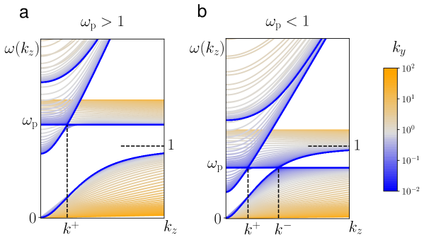
Figure 1: The dispersion relation $\omega_{n}(k_{z},k_{y})$ $(n=1,2,3,4)$ for (a) an over-dense plasma and (b) an under-dense plasma. Different values of $k_{y}$ are indicated by the color map.

Straightforward analysis shows that for a given $\omega_{\text{p}},$ the spectrum has two possible resonances, a.k.a. Weyl points, when $\boldsymbol{k}_{\perp}=0$ and $k_{z}=k^{\pm}$, where

$$k^{\pm}\equiv\dfrac{\omega_{\text{p}}}{\sqrt{1\pm\omega_{\text{p}}}}$$ (14)

are two critical wavenumbers for the given $\omega_{\text{p}}.$ We are interested in the resonance at $\boldsymbol{k}_{\perp}=0$ and $k_{z}=k^{-}$, which is between the Langmuir wave and the cyclotron wave (the R-wave near the cyclotron frequency). Obviously, this Langmuir-Cyclotron (LC) resonance or Weyl point exists when and only when the plasma is under-dense, i.e., $\omega_{\text{p}}<1$.

For a given $k_{z}$, the LC resonance occurs when $\omega_{\text{p}}=\omega_{\text{pc}}$, where

$$\omega_{\text{pc}}\equiv\dfrac{\sqrt{k_{z}^{4}+4k_{z}^{2}}-k_{z}^{2}}{2}$$ (15)

is the critical plasma frequency for the given $k_{z}$. In the parameter space of $(\omega_{\text{p}},k_{x},k_{y})$ for a fixed $k_{z}$, when moving away from the LC Weyl point $(\omega_{\text{p}},k_{x},k_{y})=(\omega_{\text{pc}},0,0)$, the distance between $\omega_{1}$ and $\omega_{2}$ will increase, i.e.,

$$\omega_{2}-\omega_{1}>0,\,\,\text{when }(\omega_{\text{p}},k_{x},k_{y})\neq(\omega_{\text{pc}},0,0).$$ (16)

Interesting topological physics happens in the neighborhood of the LC Weyl point $(\omega_{\text{p}},k_{x},k_{y})=(\omega_{\text{pc}},0,0)$. Figure 2 shows the surfaces of $\omega_{1}$ and $\omega_{2}$ as functions of $\omega_{\text{p}}$ and $k_{x}$ near the LC Weyl point. The structure is known as a Dirac cone. One important feature of the Dirac cone at the LC Weyl point is that it is tilted. Also, note that this tilted Dirac cone is in phase space since $\omega_{\text{p}}$ is a function of $x.$ This is different from condensed matter physics, where the Dirac cone is mostly in momentum space.

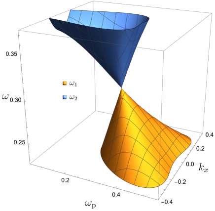
Figure 2: Tilted phase space Dirac cone in the neighborhood of the LC Weyl point $(\omega_{\text{p}},k_{x},k_{y})=(\omega_{\text{pc}},0,0)$.

Previous numerical studies and qualitative consideration [5, 6] indicated that for a given $k_{z},$ a simple 1D equilibrium that is inhomogeneous in the $x$-direction will admit the TLCW if the range of $\omega_{\text{p}}(x)$ includes $\omega_{\text{pc}}.$ In particular, we will consider the equilibrium profile displayed in Fig. 3. The profile is homogeneous in Region I $(x\leq-1)$ and Region II $(x\geq 1)$, and $\omega_{\text{p}}(x)$ monotonically decrease in the transition region $(-1\leq x\leq 1)$. The profile of $\omega_{\text{p}}(x)$ satisfies the condition

$$\omega_{\text{p}1}>\omega_{\text{p}}(0)=\omega_{\text{pc}}>\omega_{\text{p}2}\thinspace,$$ (17)

$$\omega_{\text{p}1}\equiv\omega_{\text{p}}(x\leq-1)\,,$$ (18)

$$\omega_{\text{p}2}\equiv\omega_{\text{p}}(x\geq 1).$$ (19)

The LC Weyl point locates at $x=0,$ and $\omega_{\text{p}1}$ is the plasma frequency of Region I and $\omega_{\text{p}2}$ that of Region II. Note that here $x$ is the dimensionless length normalized by $L$, the scale length of equilibrium density profile $\omega_{\text{p}}(x)$.

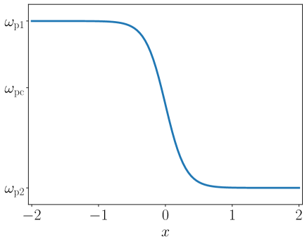
Figure 3: One-dimensional equilibrium with one transition region. The $x$ coordinate has been normalized by $L,$ the scale length of $n(x)$.

In the following analysis, we will assume $k_{z}$ is a fixed parameter unless explicitly stated otherwise.

Through the variation of $\omega_{\text{p}}(x)$, the spectrum $\omega_{n}(x,k_{x},k_{y})$ of the bulk Hamiltonian symbol $H(\boldsymbol{r},\boldsymbol{k})$ becomes a function of $x$. We defined the common gap condition for the spectra $\omega_{1}(x,k_{x},k_{y})$ and $\omega_{2}(x,k_{x},k_{y})$ as follows.

Definition 1.

The spectra $\omega_{1}(x,k_{x},k_{y})$ and $\omega_{2}(x,k_{x},k_{y})$ are said satisfying the common gap condition for parameters exterior to the ball $B_{r}^{3}\equiv\left\{(x,k_{x},k_{y})\mid x^{2}+k_{x}^{2}+k_{y}^{2}\leq r^{2}\right\}$ in the phase space of $(x,k_{x},k_{y})$, if there exists an interval $[g_{1}(r),g_{2}(r)]$ such that $\omega_{1}(x,k_{x},k_{y})<g_{1}(r)$ and $\omega_{2}(x,k_{x},k_{y})>g_{2}(r)$ for all $(x,k_{x},k_{y})\notin B_{r}^{3}.$ We call $[g_{1}(r),g_{2}(r)]$ the common gap of $\omega_{1}(x,k_{x},k_{y})$ and $\omega_{2}(x,k_{x},k_{y})$ for parameters exterior to the ball $B_{r}^{3}$.

For all the parameter space that we have explored, condition (17) implies the common gap condition of $\omega_{1}(x,k_{x},k_{y})$ and $\omega_{2}(x,k_{x},k_{y})$ for $(x,k_{x},k_{y})$ exterior to the ball of $B_{1}^{3}$. Due to the algebraic complexity of $H(\boldsymbol{r},\boldsymbol{k})$, this fact cannot be proved through a simple procedure, even though no contour example was found numerically. In Sec. VI, we will give a proof of this fact for a reduced Hamiltonian corresponding to a tilted Dirac cone in the neighborhood of the LC Weyl point. In the analysis before Sec. VI, we will take the common gap condition as an assumption.

For the 1D equilibrium with inhomogeneity in the $x$-direction, $k_{y}$ and $k_{z}$ are good quantum numbers and can be treated as system parameters. The PDO $\hat{H}(\boldsymbol{r},-\mathrm{i}\eta\nabla)$ defined in Eq. (9) reduces to

$$\hat{H}(x,-\mathrm{i}\eta\partial_{x},k_{y},k_{z})=\begin{pmatrix}\mathrm{i}\boldsymbol{e}_{z}\times&-\mathrm{i}\omega_{\text{p}}(x)&0\\ \mathrm{i}\omega_{\text{p}}(x)&0&(\mathrm{i}\eta\partial_{x},-k_{y,}-k_{z})\times\\ 0&(-\mathrm{i}\eta\partial_{x},k_{y,}k_{z})\times&0\end{pmatrix},$$ (20)

and the corresponding bulk Hamiltonian symbol is

$$H(x,k_{x},k_{y},k_{z})=\begin{pmatrix}\mathrm{i}\boldsymbol{e}_{z}\times&-\mathrm{i}\omega_{\text{p}}(x)&0\\ \mathrm{i}\omega_{\text{p}}(x)&0&(-k_{x},-k_{y,}-k_{z})\times\\ 0&(k_{x},k_{y,}k_{z})\times&0\end{pmatrix},$$ (21)

In Region I or II, the system is homogeneous, and in each region separately it is valid to speak of the homogeneous eigenmodes of $\hat{H}(x,-\mathrm{i}\eta\partial_{x},k_{y},k_{z})$, which are identical to the bulk modes of $H(x,k_{x},k_{y},k_{z})$ in that region.

The TLCW is a global eigenmode of $\hat{H}(x,-\mathrm{i}\eta\partial_{x},k_{y},k_{z})$ localized in the transition region of $-1<x<1$. Hence the name of edge mode. In Fig. 4, the numerically calculated spectrum of $\hat{H}(x,-\mathrm{i}\eta\partial_{x},k_{y},k_{z})$ is plotted as a function of $k_{y}$. The spectrum consists of three parts. The upper and lower parts are the spectrum of $\hat{H}(x,-\mathrm{i}\eta\partial_{x},k_{y},k_{z})$ that fall in the bulk bands of $H(x,k_{x},k_{y},k_{z})$ in Regions I and II. The spectrum in the middle is a single line trespassing the common band gap shared by Regions I and II. It is the TLCW. Its frequency increases monotonically with $k_{y}$, passing through $\omega_{\text{pc}}$. Such a curve of the dispersion relation for the edge mode as a function of $k_{y}$ is known as a spectral flow because it ships one eigenmode of $H(x,k_{x},k_{y},k_{z})$ from the lower band to the upper band across the band gap (see Fig. 4a). If there were two or more edge modes in the gap as in the case of oceanic equatorial waves [1, 2], there would be two or more spectral flows. In Sec. V, we will formally define spectral flow and show that the number of spectral flow reflects the topology of the plasma waves and is determined by a topological index known as the Chern number of a properly chosen manifold in the parameter space. This is why they are called topological edge modes. For the TLCW, we will show that its Chern number is one.

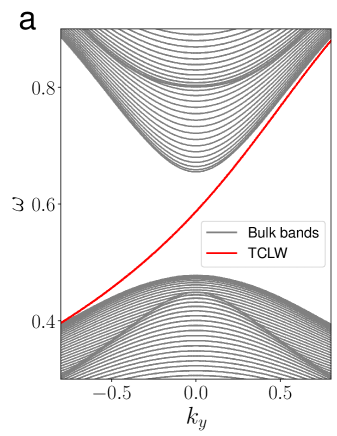
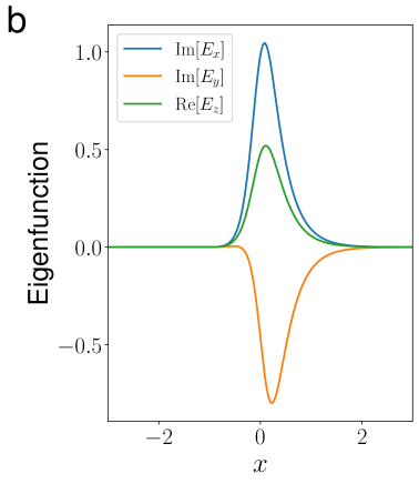
Figure 4: (a) Spectrum of $\hat{H}(x,-\mathrm{i}\eta\partial_{x},k_{y},k_{z})$ as a function of $k_{y}$. (b) The mode structure of the TLCW.

Condition (17) was identified as that for the existence of the TLCW [5, 6] by heuristically applying the bulk-edge correspondence using the numerically integrated values of the Berry curvature over the $k_{x}$-$k_{y}$ plane for the bulk modes of $H(x,k_{x},k_{y},k_{z})$ in Regions I and II. However, such an integral should not be used as a topological index for the topology waves in classical continuous media, because the topology of vector bundles over a contractible base manifold is trivial, and the $k_{x}$-$k_{y}$ plane is contractible. A detailed discussion about the trivial topology over the momentum space for classical continuous media can be found in Sec. IV.1.

In Secs. IV-VI, we show how to formulate the bulk-edge correspondence for this problem in the classical continuous media, using an index theorem of spectral flow over wavenumbers taking values in $\mathbb{R}$ established by Faure [2] and techniques of algebraic topology. We rigorously prove that there exists one TLCW when condition (17) and the common band gap condition are satisfied. After presenting additional numerical evidence of the TLCW in the next section, we will start our analytical study in Sec. IV by defining the Hermitian eigenmode bundle of plasma waves, with which the index theorem is concerned with.

III Additional numerical evidence of TLCW

In this section, we display several more examples of numerically calculated TLCW by a 1D eigenmode solver of $\hat{H}(x,-\mathrm{i}\eta\partial_{x},k_{y},k_{z})$ [5] as well as 3D time-dependent simulations [6].

The first example is the TLCW in a 1D equilibrium with two LC Wely points, as illustrated in Fig. 5. The high-density region is in the middle and the low-density region is on the two sides. When condition (17) is satisfied, we expect to observe two TLCWs, one on the right LC Weyl point and one on the left. The numerically solved spectrum of $\hat{H}(x,-\mathrm{i}\eta\partial_{x},k_{y},k_{z})$ is shown in Fig. 6, which meets the expectation satisfactorily.

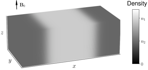
Figure 5: One-dimensional equilibrium with two Weyl points, located at the two regions where density changes.

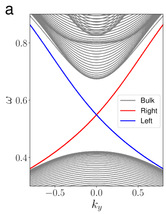
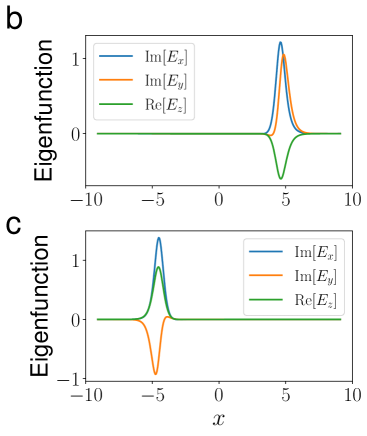
Figure 6: (a) Spectrum of $\hat{H}(x,-\mathrm{i}\eta\partial_{x},k_{y},k_{z})$ as a function of $k_{y}$. (b) The mode structure of the right TLCW. (c) The mode structure of the left TLCW.

Shown in Figs. 7 and 8 are 3D simulations of the TLCW, where the boundary between two regions are nontrivial curves in a 2D plane. In the simulations, an electromagnetic source is placed on the boundary marked by the yellow star. For the simulation in Fig. 7, the boundary is an irregular zigzag line. As anticipated, the TLCW propagates along the irregular boundary unidirectionally and without any scattering and reflection by the sharp turns. In Fig. 8, the boundary is a closed oval, and the TLCW stays on the oval boundary as expected. The propagation is again unidirectionally and without any scattering into other modes. Because $\omega_{\mathrm{p,1}}>\omega_{\mathrm{p,2}}$, the TLCW propagates counterclockwise and carries a non-zero (kinetic) angular momentum [6]. Even though the source does not carry any angular momentum, an angular-momentum-carrying surface wave is generated by the mechanism of the TLCW.

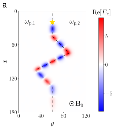
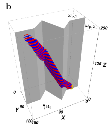
Figure 7: (a) 2D and (b) 3D simulations of the TLCW excited on a zig-zag boundary.

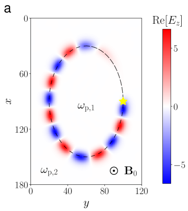
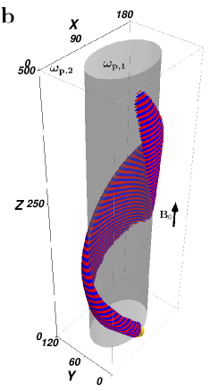
Figure 8: (a) 2D and (b) 3D simulations of the TLCW excited on an oval boundary.

IV Topology of Hermitian eigenmode bundles of plasma waves and waves in classical continuous media

The index theorem [7, 2] establishes the bulk-edge correspondence linking the nontrivial topology of the bulk mode of symbol $H$ and the spectral flow of PDO $\hat{H}$. The topology here refers to that of the Hermitian bundles of eigenmodes over appropriate regions of the parameter spaces, which we now define.

Denote the parameter space by $M$. In the present context, $M$ is the space of all possible 4-tuples $(x,k_{x},k_{z},k_{z})$. For a given $m=(x,k_{x},k_{z},k_{z})\in M$, the bulk Hamiltonian symbol $H(m)$ supports a finite number of eigenmodes. For the plasma wave operator defined by Eq. (21), there are 9 eigenmodes as explained in Sec. II. But, most of the discussion and results in this section are not specific to the plasma waves and remain valid for a general bulk Hamiltonian symbol $H(m)$ in continuous media with 1D inhomogeneity. When there is no degeneracy for a given eigenfrequency, all eigenvectors corresponding to the eigenfrequency form a 1D complex vector space.

Definition 2.

Let $Q\subset M$ be a subset of the parameter space that forms a manifold with or without boundary. If the $j$-th eigenmode is not degenerate over $Q$, then the space of disjointed union of all eigenvectors of $\psi_{j}(q)$ at all $q\in Q$ forms a 1D complex line bundle

$$\pi_{j}:E_{j}\rightarrow Q$$ (22)

over $Q$. With the standard Hermitian form

$$\left\langle u,w\right\rangle\equiv u\cdot\bar{w},$$ (23)

for all $u,w\in\pi_{j}^{-1}(q)$ and $q\in Q,$ $E_{j}\rightarrow Q$ is also a Hermitian bundle. It will be called the Hermitian line bundle of the $j$-th eigenmode of the bulk Hamiltonian symbol $H(m)$ over $Q$.

If both the $l$-th eigenmode and the $j$-th eigenmode are non-degenerate over $Q,$ the Whitney sum of $E_{l}\rightarrow Q$ and $E_{j}\rightarrow Q$ defines the Hermitian line bundle of the $l$-th and the $j$-th eigenmodes,

$$E_{\{l,j\}}\equiv E_{l}\oplus E_{j}$$ (24)

with the Hermitian form defined as

$$\left\langle\boldsymbol{u},\boldsymbol{v}\right\rangle\equiv u_{l}\cdot\bar{w}_{l}+u_{j}\cdot\bar{w}_{j},$$ (25)

for all $\boldsymbol{u}=(u_{l},u_{j}),\boldsymbol{w}=(w_{l},w_{j})$, where $u_{l},w_{l}\in\pi_{l}^{-1}(q)$ and $u_{j},w_{j}\in\pi_{j}^{-1}(q)$. Similarly, Hermitian bundle of a set of eigenmodes indexed by set $J$ is defined as

$$E_{J}\equiv\oplus_{j\in J}E_{j}\thinspace,$$ (26)

if for each $j\in J,$ the $j$-th eigenmode is not degenerate over $Q$. In general, $E_{J}$ can be defined when degeneracy exists only between indices in $J$, but we will not use this structure in the present study.

The current study is concerned with the topology of the Hermitian line bundles $E_{j}\rightarrow Q$. In particular, we would like to know when the bundle is trivial, i.e., a global product bundle over $Q$, and when it is not. If nontrivial, it is desirable to calculate the Chern classes of the bundle to measure how twisted it is. For the Hermitian line bundles of eigenmodes of plasma waves, we will show in Secs. V and VI that the topological index of the $E_{1}$ bundle over a properly chosen non-contractible, compact manifold in phase space $Q$, calculated from its first Chern class $C_{1}(E_{1})$, determines the number of TLCWs at the transition region.

For Hermitian bundles, the associated principal bundles are $U(n)$ bundles and each Chern class $C_{j}$ is a de Rham cohomology class of the base manifold constructed from a curvature 2-form of the bundles. According to the Chern-Weil theorem, different connections for the bundles yield the same de Rham cohomology classes on the base manifold. In the present study, it is only necessary to calculate the first Chern class, and the following result is useful,

$$C_{1}(E_{J})=\sum_{j\in J}C_{1}(E_{j})\,.$$ (27)

The right-hand side of Eq. (27) is relatively easy to calculate because each $E_{j}$ is a Hermitian line bundle, whose first Chern class is given by

$$C_{1} =\dfrac{\mathrm{i}}{2\pi}\theta,$$ (28)

$$\theta =\mathrm{d}\chi,$$ (29)

where $\theta$ is a curvature 2-form and $\chi$ is a connection. As mentioned above, different connections will generate the same $C_{1}$ class. Nevertheless, the Hermitian line bundle is endowed with natural connection

$$\chi=\left\langle w,\mathrm{d}w\right\rangle,$$ (30)

which is a $u(1)$-valued local 1-form in each trivialization patch. This natural connection for the Hermitian line bundle is known as the Berry connection in condensed matter physics or the Simon connection .

IV.1 Trivial topology of plasma waves in momentum space

In terms of topological properties, there is a major difference between condensed matters and classical continuous media such as plasmas and fluids. The momentum space, or wavenumber space, of typical condensed matters is the Brillouin zone, which is non-contractible due to the periodicity of the lattices. On the contrary, the wavenumber space in plasmas and fluids is contractible, and it is a well-known fact that vector bundles over a contractible manifold are trivial. Here, a topological manifold $M$ is called contractible if it is of the same homotopy type of a point, i.e., there exist a point $x_{0}$ and continuous maps $f:M$$\rightarrow\{x_{0}\}$ and $g:\{x_{0}\}\rightarrow M$ such that $f\circ g$ is homotopic to identity in $\{x_{0}\}$ and $g\circ f$ is homotopic to identity in $M.$ Because of its importance to the continuous media in classical physics, we formalize this result as a theorem.

Theorem 3.

Let $Q$ be a subset of the parameter space $M$ for a bulk Hamiltonian symbol $H$. If the $j$-th eigenmode is non-degenerate on $Q$, and $Q$ is a contractible manifold, then the Hermitian line bundle $E_{j}\rightarrow Q$ is trivial. In particular, the n-th Chern class $C_{n}($$E_{j}\rightarrow Q)=0$ for $n\geq 1.$

Note that Theorem 3 holds for any bulk Hamiltonian symbol. For the $H(\boldsymbol{r},\boldsymbol{k})$ defined in Eq. (13) and the $H(x,k_{x},k_{y},k_{z})$ defined in Eq. (21) for plasma waves, a more specific result is available as a direct corollary of Theorem 3.

Theorem 4.

For the bulk Hamiltonian symbol $H(\boldsymbol{r},\boldsymbol{k})$ defined in Eq. (13) for plasma waves, when $k_{z}\neq k^{\pm},$ the Hermitian line bundle of all eigenmodes over the perpendicular wavenumber plane $Q_{k_{\perp}}=\{(k_{x},k_{y})\mid k_{x}\in\mathbb{R},\thinspace k_{y}\in\mathbb{R}\}=\mathbb{R}^{2}$ are trivial. In particular, $C_{n}(E_{j}\rightarrow Q_{k_{\perp}})=0$ for $n\geq 1$ and $-4\leq j\leq 4.$

The fact that $C_{n}(E_{j}\rightarrow Q)$ vanishes when $Q$ is contractible is expected after all because $C_{n}$ is the de Rham cohomology class of the base manifold. But Theorem 4 is important. It tells us that the plasma wave topology over the $k_{x}$-$k_{y}$ plane is trivial if $k_{z}\neq k^{\pm}.$ Nontrivial topology of plasma wave bundles occurs only over non-contractible parameter manifolds, for example, over an $S^{2}$ surface in the phase space of $(x,k_{x},k_{y})$, as we will show in Sec. IV.2.

Before leaving this subsection, we would like to point out that in recent studies of wave topology in classical continuous media, much effort has been made to calculate “topological indices” or “Chern numbers” of the eigenmode bundles over the contractible $k_{x}$-$k_{y}$ plane. This type of effort is characterized by the attempt to evaluate the integration of the Berry curvature or various modified versions thereof over the $k_{x}$-$k_{y}$ plane. The difficulties involved were often attributed to the fact that the $k_{x}$-$k_{y}$ plane is not compact. As we see from Theorems 3 and 4, when the wave bundle is well-defined over the entire $k_{x}$-$k_{y}$ plane, its topology is trivial. In these cases, the non-compactness of the $k_{x}$-$k_{y}$ plane is irrelevant, so is whether an integer or non-integer index can be designed.

IV.2 Nontrivial plasma wave topology in phase space

In the present context, the ultimate utility of the topological property of the eigenmode bundles of the bulk Hamiltonian symbol $H$ is to predict the existence of the topological edge modes of the global Hamiltonian PDO $\hat{H}.$ For this purpose, the proper plasma wave eigenmode bundles are over the 2D sphere in the parameter space of $(x,k_{x},k_{y})$ for the $H(x,k_{x},k_{y},k_{z})$ defined in Eq. (21),

$$S_{1}^{2}=\left\{(x,k_{x},k_{y})\mid x^{2}+k_{x}^{2}+k_{y}^{2}=1\right\}=\partial B_{1}^{3},$$ (31)

where $B_{1}^{3}$ is the 3D ball with radius $r=1$.

One indicator of nontrivial topology, or twist, of a wave eigenmode bundle over $S_{1}^{2}$ is the number of zeros a nontrivial section must have, akin to the situation of hairy ball theorem for the tangent bundle of $S^{2}$. To include the possibilities of repeated zeros, we follow Frankel [27] to define the index of an isolated zero point $z$ of a section $u$ of a Hermitian line bundle as follows.

Definition 5.

Let $z$ be an isolated zero of a section $u$ that has a finite number of zeros. Select a normalized local frame $e$ for the Hermitian line bundle in the neighborhood of $z$. The normalized section near $z$, but not at $z,$ can be expressed as $u/\mid u\mid=e\text{exp}(\mathrm{i}\alpha).$ The index at $z$ is defined to be

$$j_{u}(z)\equiv\frac{1}{2\pi}\int_{\partial D}\mathrm{d}\alpha,$$ (32)

where $D$ is a small disk containing $z$ on $S_{1}^{2}$ with orientation pointing away from $S_{1}^{2},$ and the orientation of $\partial D$ is induced from that of $D$. The index of the section $u$ is the sum of indices at all zeros $z_{l}$ of $u,$

$$\text{Ind}(u)\equiv\sum_{l}j_{u}(z_{l}).$$ (33)

Note that for each isolated zero $z$, the local frame $e$ selected in the neighborhood of $z$ is not vanishing at $z$. The index $j_{u}(z)$ intuitively measures how many turns the phase of $u$ increases relative to $e$ at $z$ over one turn on $\partial D$. In general, $e$ is only a local frame instead of a global frame, otherwise the bundle is trivial.

The following theorem of Chern relates the index of a nontrivial section to the first Chern class over $S^{2}$ [27].

Theorem 6.

[Chern] Let $E$ be a Hermitian line bundle over a closed orientable 2D surface $S^{2}$. Let $u:$$S^{2}\rightarrow E$ be a section of $E$ with a finite number of zeros. Then the integral of the 1st Chern class $C_{1}$ over $S^{2}$ is an integer that is equal to the index of the section $u,$ i.e.,

$$n_{c}\equiv\int_{S^{2}}C_{1}(E\rightarrow S^{2})=\mathrm{Ind}(u).$$

Here, $n_{c}$ is known as the first Chern number. Since the present study only involves the first Chern number, it is denoted by $n_{c}$ instead of $n_{c_{1}}.$ The first Chern number of the $j$-th eigenmode bundle over $S_{1}^{2}$ is denoted by $n_{cj}$. In Sec. V, the first Chern number $n_{c1}$ of the plasma wave eigenmode bundle $E_{1}$ over $S_{1}^{2}$ will be linked to the spectral flow index of $\hat{H}(x,-\mathrm{i}\eta\partial_{x},k_{y},k_{z})$ using Faure’s index theorem [2]. To facilitate the calculation of $n_{cj}$ over $S_{1}^{2}$, we establish the following general facts about eigenmode bundles in continuous media, including plasma wave eigenmode bundles.

Definition 7.

Let $\pi_{1}:E_{1}\rightarrow P$ and $\pi_{2}:E_{2}\rightarrow Q$ be two vector bundles. A diffeomorphism $\phi:E_{1}\rightarrow E_{2}$ is called an isomorphism if for every $p\in P$, $\exists$ $q\in Q$ such that $\phi\circ\pi_{1}^{-1}(p)\subset\pi_{2}^{-1}(q)$ and $\phi:\pi_{1}^{-1}(p)\rightarrow\pi_{2}^{-1}(q)$ is a vector space isomorphism. If an isomorphism exists, $E_{1}$ and $E_{2}$ are isomorphic, denoted as $E_{1}\simeq E_{2}.$

Note that the base manifolds $P$ and $Q$ in the above definition can be identical or different.

Definition 8.

Let $f:P\rightarrow Q$ is a smooth map between differential manifolds $P$ and $Q,$ and $\pi_{2}:E\rightarrow Q$ a vector bundle over $Q$. The pullback bundle $\pi_{1}:f^{*}E\rightarrow P$ is defined to be

$$f^{*}E=\left\{(p,e)\in P\times E\mid p\in P,\,e\in E,\,f(p)=\pi_{2}(e)\right\}.$$ (34)

The standard manifold and vector bundle structure of $f^{*}E$ can be formally established. For example, see Ref. [28]. Note that the pullback bundle is defined as a pullback set and this mechanism does not define a map from $E$ to $f^{*}E$ because $f$ is not in general invertible. On the other hand, when $f$ is invertible, a pullback map from $E$ to $f^{*}E$ can be defined by a similar mechanism as follows.

Definition 9.

Let $f:P\rightarrow Q$ is a diffeomorphism between differential manifolds $P$ and $Q,$ and $\pi_{2}:E\rightarrow Q$ a vector bundle over $Q$. The pullback map $f^{\dagger}$ is defined to be

$$f^{\dagger}: E\rightarrow f^{*}E,$$ (35)

$$e\mapsto(f^{-1}\circ\pi_{2}(e),e).$$

When $f$ is a diffeomorphism, $f^{\dagger}(E)=f^{*}E.$

We will use the following theorem known as homotopy induced isomorphism [29].

Theorem 10.

[Homotopy induced isomorphism] Let $f_{0}$ and $f_{1}$ are two homotopic maps between manifolds $P$ and $Q$. For a vector bundle $E\rightarrow Q$, the pullback bundles $f_{0}^{*}E$ and $f_{1}^{*}E$ over $P$ are isomorphic.

Theorem 3 is a direct corollary of Theorem 10.

Theorem 11.

Let $f:P\rightarrow Q$ is a diffeomorphism between differential manifolds $P$ and $Q$, and $\pi_{2}:E\rightarrow Q$ a vector bundle over $Q$. The pullback map $f^{\dagger}$ is an isomorphism between $E$ and $f^{*}E$.

Proof.

According to Definition 7, it suffices to prove that (i) $f^{\dagger}:E\rightarrow f^{*}E$ is a diffeomorphism and (ii) $\forall q\in Q,$ $\exists p\in P$ such that $f^{\dagger}\circ\pi_{2}^{-1}(q)\subset\pi_{1}^{-1}(p)$ and $f^{\dagger}:\pi_{2}^{-1}(q)\mapsto\pi_{1}^{-1}(p)$ is an isomorphism of vector space.

Since $f^{\dagger}(e)=(f^{-1}\circ\pi_{2}(e),e)$ and both $f^{-1}$ and $\pi_{2}$ are smooth, $f^{\dagger}$ is smooth. By construction, $f^{\dagger}$ is smoothly invertible. Thus, $f^{\dagger}$ is a diffeomorphism. To prove (ii), we utilize a local trivialization. For $\forall q\in Q$, let $U$ be an open set containing $q$ in the open cover of $Q$ for the local trivialization of $E\rightarrow Q$. Locally, $E$ is a production $U\times V.$ In particular, $\pi_{2}^{-1}(q)=\{q\}\times V$ and

$$f^{\dagger}:(q,v)\mapsto\left(p=f^{-1}\circ\pi_{2}(q,v)=f^{-1}(q),(q,v)\right).$$ (36)

For this fixed $q,$

$$f^{\dagger}\circ\pi_{2}^{-1}(q) =f^{\dagger}\left(\left\{(q,v)\mid v\in V\right\}\right)=\left\{\left(p,(q,v)\right)\mid p=f^{-1}(q),v\in V\right\}$$

$$=\left\{\left(p,(q,v)\right)\mid f(p)=\pi_{2}(q,v),v\in V\right\}=\pi_{1}^{-1}(p).$$ (37)

Also, $f^{\dagger}:(q,v)\mapsto\left(p,(q,v)\right)$ for the fixed $q$ and $p=f^{-1}(q)$ is an isomorphism. Thus, $f^{\dagger}$ is an isomorphism and $E\simeq f^{*}E$. ∎

The following is the main theorem of this paper, which will enable us to analytical calculate the topological index for the TLCW. In a parameter space that is $\mathbb{R}^{3}$, denote by $S_{r}^{2}=\left\{q=(q_{1,}q_{2,}q_{3})\mid q_{1}^{2}+q_{2}^{2}+q_{3}^{2}=r^{2}\right\}$ the sphere of radius $r$, and by $Sh_{(a,b)}\equiv\left\{q=(q_{1,}q_{2,}q_{3})\mid a^{2}\leq q_{1}^{2}+q_{2}^{2}+q_{3}^{2}\leq b^{2}\right\}$ the 3D shell with inner radius $a$ and outer radius $b$.

Theorem 12.

[Boundary isomorphism] Let $E\rightarrow Sh_{(a,b)}$ be a Hermitian line bundle defined over a shell $Sh_{(a,b)}$ in a parameter space that is $\mathbb{R}^{3}$.

(i) The bundles obtained by restricting $E$ over $S_{a}^{2}$ and $S_{b}^{2}$ are isomorphic, i.e., $E\rightarrow S_{a}^{2}\simeq E\rightarrow S_{b}^{2}$.

(ii) Bundles $E\rightarrow S_{a}^{2}$ and $E\rightarrow S_{b}^{2}$ have the same first Chern number, i.e., $n_{c}\left(E\rightarrow S_{a}^{2}\right)=n_{c}\left(E\rightarrow S_{b}^{2}\right)$.

Proof.

To prove (i), construct the following continuous class of compressing maps on $Sh_{(a,b)}$,

$$f_{\epsilon}: Sh_{(a,b)}\rightarrow Sh_{(a,b)}\thinspace,$$ (38)

$$p\mapsto\epsilon p+(1-\epsilon)\frac{ap}{\left|p\right|},\thinspace 0\leq\epsilon\leq 1.$$

As $\epsilon$ decreases from $1$ to $0$ continuously, $f_{\epsilon}$ compresses the shell towards the inner sphere $S_{a}^{2}$. $f_{1}$ is the identify map, $f_{0}$ crashes the shell onto $S_{a}^{2},$ and $f_{1}$ and $f_{0}$ are homotopic. According to Theorem 10,

$$f_{1}^{*}E\simeq f_{0}^{*}E\>.$$ (39)

Restricting both sides of Eq. (39) to $S_{b}^{2}$ leads to

$$E\mid_{S_{b}^{2}}=\left(f_{1}^{*}E\right)\mid_{S_{b}^{2}}\simeq\left(f_{0}^{*}E\right)\mid_{S_{b}^{2}}=f_{0}^{*}\left(E\mid_{S_{a}^{2}}\right)\mid_{S_{b}^{2}}.$$ (40)

Denote by $f_{0r}$ the restriction of $f_{0}$ on $S_{b}^{2},$ i.e.,

$$f_{0r}: S_{b}^{2}\rightarrow S_{a}^{2}\thinspace,$$

$$p\mapsto f_{0}(p).$$ (41)

Obviously, $f_{0r}$ is a diffeomorphism, and according to Theorem 11,

$$f_{0}^{*}\left(E\mid_{S_{a}^{2}}\right)\mid_{S_{b}^{2}}=f_{0r}^{*}\left(E\mid_{S_{a}^{2}}\right)\simeq E\mid_{S_{a}^{2}}.$$ (42)

Therefore,

$$E\rightarrow S_{b}^{2}=E\mid_{S_{b}^{2}}\simeq E\mid_{S_{a}^{2}}=E\rightarrow S_{a}^{2}\,.$$ (43)

For (ii), we have

$$f_{0r}^{*}\left(C_{1}\left(E\rightarrow S_{a}^{2}\right)\right)=C_{1}\left(f_{0r}^{*}\left(E\rightarrow S_{a}^{2}\right)\right)=C_{1}\left(E\rightarrow S_{b}^{2}\right),$$

where the first equal sign is the naturality property of characteristic classes. The second equal sign is due to the fact that $f_{0r}^{*}\left(E\rightarrow S_{a}^{2}\right)$ and $E\rightarrow S_{b}^{2}$ are two isomorphic bundles on $S_{b}^{2}$, and thus have the same Chern classes. The first Chern number on $E\rightarrow S_{b}^{2}$ is

$$n_{c}\left(E\rightarrow S_{b}^{2}\right) =\int_{S_{b}^{2}}C_{1}\left(E\rightarrow S_{b}^{2}\right)$$ (44)

$$=\int_{S_{b}^{2}}f_{0r}^{*}\left(C_{1}\left(E\rightarrow S_{a}^{2}\right)\right)$$

$$=\int_{S_{a}^{2}}C_{1}\left(E\rightarrow S_{a}^{2}\right)=n_{c}\left(E\rightarrow S_{a}^{2}\right),$$

where the integral on $S_{b}^{2}$ is evaluated on $S_{a}^{2}$ via the pullback mechanism in the third equal sign. ∎

Theorem 12 says that when the Hermitian line bundle $E$ is defined on $Sh(a,b),$ $E\rightarrow S_{a}^{2}$ and $E\rightarrow S_{b}^{2}$ are isomorphic bundles and have the same first Chern number. Around an isolated Weyl point, the Hermitian line bundle is well defined except at the Weyl point, Theorem 12 states that all closed surfaces surrounding the Weyl point have the same first Chern number, which can be viewed as the topological charge associated with this isolated Weyl point in phase space (see Fig. 9).

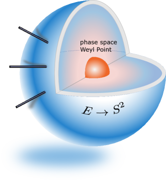
Figure 9: Topological charge of waves in classical continuous media. Around an isolated Weyl point, all closed surfaces surrounding the Weyl point have the same first Chern number, which can be viewed as the topological charge associated with this isolated Weyl point in phase space.

We also need the following results for the first Chern class for the plasma wave eigenmode bundles. They can be established straightforwardly.

Lemma 13.

For the 9 bulk eigenmode bundles of the plasma waves specified by Hamiltonian symbol $H(\boldsymbol{r},\boldsymbol{k})$ defined in Eq. (13), the following identities for the first Chern class holds over a general base manifold for the bundles:

$$C_{1}\left(\oplus_{j=1}^{4}E_{j}\right) =C_{1}\left(\oplus_{j=-4}^{-1}E_{j}\right),$$ (45)

$$C_{1}\left(\oplus_{j=-4}^{4}E_{j}\right) =0,$$ (46)

$$C_{1}\left(E_{0}\right) =0,$$ (47)

$$C_{1}\left(\oplus_{j=-4}^{1}E_{j}\right) =C_{1}\left(E_{1}\right).$$ (48)

V TLCW predicted by Faure’s index theorem and algebraic topological analysis

V.1 Faure’s Index theorem for TLCW

In condensed matter physics, the bulk-edge correspondence states that the gap Chern number equals the number of edge modes in the gap. Mathematically, the correspondence had been rigorously proved as the Atiyah-Patodi-Singer (APS) index theorem [7] for spectral flows over $S^{1}$, which corresponds to the momentum parameter $k_{y}$ in the direction with spatial translation symmetry of a periodic lattice. However, for waves in classical continuous media, including waves in plasmas, the $k_{y}$ parameter is not periodic, and it takes value in $\mathbb{R}$. Therefore, the APS index theorem proved for spectral flow over $S^{1}$ is not applicable for waves in continuous media without modification. Recently, Faure [2] formulated an index theorem for spectral flows over $\mathbb{R}$-valued $k_{y}$, which links the spectral flow index to the gap Chern number of the eigenmode bundle over a 3D ball in the phase space of $(x,k_{x},k_{y}).$ Faure’s index theorem applies to waves in classical continuous media. In this section, we apply Faure’s index theorem and Theorem 12 to prove the existence of TLCW. For the bulk Hamiltonian symbol $H(x,k_{x},k_{y},k_{z})$ defined in Eq. (21), the global Hamiltonian PDO $\hat{H}(x,-\mathrm{i}\eta\partial_{x},k_{y},k_{z})$ defined in Eq. (20), and the 1D equilibrium profile specified by Eq. (17), we have the following theorems and definition adapted from Faure [2].

Theorem 14.

For a fixed $k_{z}$, assume that $[g_{1},g_{2}]$ is the common gap of $\omega_{1}(x,k_{x},k_{y})$ and $\omega_{2}(x,k_{x},k_{y})$ for parameters exterior to the ball $B_{1}^{3}$. For any $\lambda>0,$ there exists $\eta_{0}>0$ such that

(i) for all $\eta<\eta_{0}$ and $k_{y}\in[-1-\lambda,1+\lambda]$, $\hat{H}(x,-\mathrm{i}\eta\partial_{x},k_{y},k_{z})$ has no or discrete spectrum in the gap of $[g_{1}+\lambda,g_{2}-\lambda]$ that depend on $\eta$ and $k_{y}$ continuously;

(ii) for all $\eta<\eta_{0}$, $\hat{H}(x,-\mathrm{i}\eta\partial_{x},k_{y},k_{z})$ has no spectrum in $[g_{1}-\lambda,g_{2}+\lambda]$ at $k_{y}=\pm(1+\lambda).$

Proof.

This theorem is a special case of Theorem 2.2 in Faure [2]. ∎

Theorem 14 states that the spectrum of $\hat{H}(x,-\mathrm{i}\eta\partial_{x},k_{y},k_{z})$ in the common gap $[g_{1}+\lambda,g_{2}-\lambda]$, if any, must consist of discrete dispersion curves parameterized by $k_{y}$. Theorem 14 also stipulates the following “traffic rules” for the flow of the spectrum. The dispersion curves cannot enter or exit the rectangle region $[-1-\lambda,1+\lambda]\times[g_{1}+\lambda,g_{2}-\lambda]$ on the $k_{y}$-$\omega$ plane from the left or right sides. They can only enter or exit through the upper or lower sides (see Fig. 10). Intuitively, a spectral flow is a dispersion curve of $\hat{H}(x,-\mathrm{i}\eta\partial_{x},k_{y},k_{z})$ that can trespass the rectangle. It flows between the lower band and the upper band, as if transporting one eigenmode upward or downward through the spectral gap of $H(x,k_{x},k_{y},k_{z})$ for parameters exterior to the ball $B_{1}^{3}$. We now formally define the spectral flow and spectral flow index.

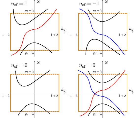
Figure 10: Illustration of possible spectral flows of $\hat{H}(x,-\mathrm{i}\eta\partial_{x},k_{y},k_{z})$ in the common gap $[g_{1}+\lambda,g_{2}-\lambda]$. Theorem 14 stipulates the “traffic rules” for the flow of the spectrum. Red curves are spectral flows with index $1$, and blue curves are spectral flows with index $-1.$

Definition 15.

For a fixed $k_{z}$, assume that $[g_{1},g_{2}]$ is the common gap of $\omega_{1}(x,k_{x},k_{y})$ and $\omega_{2}(x,k_{x},k_{y})$ for parameters exterior to the ball $B_{1}^{3}$. A spectral flow is a smooth dispersion curve $\omega=f(k_{y},\eta)$ of $\hat{H}(x,-\mathrm{i}\eta\partial_{x},k_{y},k_{z})$ satisfying the following condition: For any $\lambda>0,$ there exists a $\eta_{0}>0$ such that either (i) for all $\eta<\eta_{0}$, $f(-1-\lambda,\eta)<g_{1}+\lambda$ and $f(1+\lambda,\eta)>g_{2}-\lambda$ or (ii) for all $\eta<\eta_{0}$, $f(-1-\lambda,\eta)>g_{2}-\lambda$ and $f(1+\lambda,\eta)<g_{1}+\lambda$. For case (i), its index is $1$. For case (ii), its index is $-1$. The spectral flow index $n_{\text{sf}}$ of $\hat{H}(x,-\mathrm{i}\eta\partial_{x},k_{y},k_{z})$ is the summation of indices of all its spectral flows.

In the present context, a spectral flow of $\hat{H}(x,-\mathrm{i}\eta\partial_{x},k_{y},k_{z})$ is a TLCW. But Theorem 14 and Definition 15 are valid for any generic $\hat{H}$.

A few possible spectral flow configurations are illustrated in Fig. 10. Strictly speaking, $n_{\text{sf}}$ is not necessarily the total number of all possible upward and downward spectral flows of $\hat{H}(x,-\mathrm{i}\eta\partial_{x},k_{y},k_{z})$. It is the net number of upward spectral flows.

For plasma waves, the following theorem links the number of TLCWs to the first Chern number of the $E_{1}$ eigenmode bundle over a non-contractible, compact surface in the phase space of $(x,k_{x},k_{y}).$

Theorem 16.

For a fixed $k_{z},$ assume that the common gap condition for parameters exterior to the ball $B_{1}^{3}\equiv\left\{(x,k_{x},k_{y})\mid x^{2}+k_{x}^{2}+k_{y}^{2}\leq 1\right\}$ is satisfied for the spectra $\omega_{1}(x,k_{x},k_{y},k_{z})$ and $\omega_{2}(x,k_{x},k_{y},k_{z})$ of $H(x,k_{x},k_{y},k_{z})$. The spectral flow index of $\hat{H}(x,-\mathrm{i}\eta\partial_{x},k_{y},k_{z})$ in the gap equals the Chern number $n_{c}\left(E_{1}\rightarrow S_{1}^{2}\right)$ of the $E_{1}$ eigenmode bundle of $H(x,k_{x},k_{y},k_{z})$ over $S_{1}^{2}\equiv\left\{(x,k_{x},k_{y})\mid x^{2}+k_{x}^{2}+k_{y}^{2}\leq 1\right\}$, i.e., $n_{\text{sf}}=n_{c}\left(E_{1}\rightarrow S_{1}^{2}\right)$.

Proof.

This theorem is a direct specialization of Theorem 2.7 formulated by Faure in Ref. [2], which states that when a spectral gap exists between $\omega_{l}$ and $\omega_{l+1}$ of a bulk Hamiltonian for all parameters exteriors to $B_{r}^{3}$, the spectral flow index $n_{\text{sf}}$ of the corresponding PDO in the gap equals the gap Chern number $n_{c}\left(\oplus_{j\leq l}E_{j}\rightarrow S_{r}^{2}\right)$. For the plasma waves satisfying the common gap condition stated, $l=1$ and

$$n_{\text{sf}}=n_{c}\left(\oplus_{j\leq 1}E_{j}\rightarrow S_{1}^{2}\right)=n_{c}\left(E_{1}\rightarrow S_{1}^{2}\right),$$

where use is made of Lemma 13. ∎

V.2 Index calculation of TLCW using algebraic topological techniques

Theorem 16 links the number of TLCWs, or the spectral flow index of $\hat{H}(x,-\mathrm{i}\eta\partial_{x},k_{y},k_{z})$, to the Chern number $n_{c}\left(E_{1}\rightarrow S_{1}^{2}\right)$ of the $E_{1}$ eigenmode bundle of $H(x,k_{x},k_{y},k_{z})$ over $S_{1}^{2}\equiv\left\{(x,k_{x},k_{y})\mid x^{2}+k_{x}^{2}+k_{y}^{2}\leq 1\right\}$. However, it is not an easy task to calculate $n_{c}\left(E_{1}\rightarrow S_{1}^{2}\right)$ either analytically or numerically. Here, we use the algebraic topological tools developed in Sec. IV.2 to analytically calculate $n_{c}\left(E_{1}\rightarrow S_{1}^{2}\right).$

Because for the 1D equilibrium profile specified by Eq. (17), the LC Weyl point only occurs at $x=0,$ and the eigenmode bundle $E_{1}$ is well-defined in $B_{1}^{3}/(0,0,0)$, we can invoke Theorem 12 to calculate $n_{c}\left(E_{1}\rightarrow S_{1}^{2}\right)$ as

$$n_{c}\left(E_{1}\rightarrow S_{1}^{2}\right)=\lim_{\delta\rightarrow 0^{+}}n_{c}\left(E_{1}\rightarrow S_{\delta}^{2}\right).$$ (49)

The right-hand side of Eq. (49) is the first Chern number of the $E_{1}$ bundle over an infinitesimal sphere surrounding the Weyl point in the phase space of $(x,k_{x},k_{y})$, and it can be analytically evaluated using Taylor expansion at the Weyl point as follows.

At the LC Weyl point $(x,k_{x},k_{y})=(0,0,0)$, the spectrum and eigenmodes of $H(x,k_{x},k_{y},k_{z})$ can be solved analytically. Denote by $\left(\omega_{j0},\psi_{j0}\right)$ the $j$-th eigenmode. At this point, two of the eigenmodes with positive frequencies resonant,

$$\omega_{10}=\omega_{20}=\omega_{\text{pc}}=\dfrac{\sqrt{k_{z}^{4}+4k_{z}^{2}}-k_{z}^{2}}{2},$$ (50)

and the corresponding eigenmodes are

$$\psi_{10} =\left(0,0,-\frac{\mathrm{i}}{\sqrt{2}},0,0,\frac{1}{\sqrt{2}},0,0,0\right)^{\mathrm{T}},$$

$$\psi_{20} =\left(\mathrm{i}k_{z},-k_{z},0,\frac{\omega_{\text{pc}}}{k_{z}},\mathrm{i}\frac{\omega_{\text{pc}}}{k_{z}},0,-\mathrm{i},1,0\right)^{\mathrm{T}},$$

where $\psi_{10}$ is the Langmuir wave and $\psi_{20}$ is the cyclotron wave. In the infinitesimal neighborhood of the Weyl point, $k_{x}\sim k_{y}\sim x\sim\delta$,

$$H(x,k_{x},k_{y},k_{z}) =H_{0}+\delta H,$$ (51)

$$H_{0}(x,k_{x},k_{y},k_{z}) =\begin{pmatrix}\mathrm{i}\boldsymbol{e}_{z}\times&-\mathrm{i}\omega_{\text{pc}}&0\\ \mathrm{i}\omega_{\text{pc}}&0&(0,0,-k_{z})\times\\ 0&(0,0,k_{z})\times&0\end{pmatrix},$$ (52)

$$\delta H(x,k_{x},k_{y},k_{z}) =\begin{pmatrix}0&-\mathrm{i}\omega_{\text{p}}^{\prime}(x)x&0\\ \mathrm{i}\omega_{\text{p}}^{\prime}(x)x&0&(-k_{x},-k_{y,}0)\times\\ 0&(k_{x},k_{y,}0)\times&0\end{pmatrix}.$$ (53)

We can express $H$ in the basis of $\psi_{j0}$ $(-4\leq j\leq 4)$. But for modes with $\delta\omega=$$\omega-\omega_{\text{pc}}\sim\delta$, $H$ can approximated by the expansion using $\psi_{10}$ and $\psi_{20}$ only, and reduces to a $2\times 2$ matrix,

$$H_{2} (x,k_{x},k_{y},k_{z}):=\begin{pmatrix}\psi_{10}^{\dagger}H\psi_{10}&\psi_{10}^{\dagger}H\psi_{20}\\ \psi_{20}^{\dagger}H\psi_{10}&\psi_{20}^{\dagger}H\psi_{20}\end{pmatrix}=\begin{pmatrix}\omega_{\text{pc}}+\delta\omega_{\text{p}}&\dfrac{-k_{x}-\mathrm{i}k_{y}}{\sqrt{2}\alpha}\\[10.0pt] \dfrac{-k_{x}+\mathrm{i}k_{y}}{\sqrt{2}\alpha}&\omega_{\text{pc}}-\dfrac{4\omega_{\text{pc}}}{\alpha^{2}}\delta\omega_{\text{p}}\end{pmatrix},$$ (54)

$$\alpha \equiv\sqrt{4+3k_{z}^{2}-k_{z}\sqrt{4+k_{z}^{2}}}\thinspace,\quad\delta\omega_{\text{p}}=-\beta x\thinspace,\quad\beta\equiv\left|\dfrac{\mathrm{d}\omega_{\text{p}}}{\mathrm{d}x}\right|_{x=0}\geq 0,$$ (55)

where we used the fact that the equilibrium profile $\omega_{\mathrm{p}}(x)$ selected in Eq. (17) decreases monotonically. The eigen system of $H_{2}$ can be solved straightforwardly. The two eigenfrequencies of $H_{2}$ are

$$\omega_{1} =\omega_{\text{pc}}-\frac{\beta}{2}\left(1-\frac{4\omega_{\text{pc}}}{\alpha^{2}}\right)x-\gamma\thinspace,$$ (56)

$$\omega_{2} =\omega_{\text{pc}}-\frac{\beta}{2}\left(1-\frac{4\omega_{\text{pc}}}{\alpha^{2}}\right)x+\gamma\thinspace,$$ (57)

$$\gamma \equiv\sqrt{\frac{k_{x}^{2}+k_{y}^{2}}{2\alpha^{2}}+\frac{x^{2}\beta^{2}}{4}\left(1+\frac{4\omega_{\text{pc}}}{\alpha^{2}}\right)^{2}}\thinspace.$$ (58)

The corresponding eigenmodes, expressed in the basis of $\psi_{10}$ and $\psi_{20}$ , are

$$\tilde{\psi}_{1} =\left(\alpha\beta\left(1+\frac{4\omega_{\text{pc}}}{\alpha^{2}}\right)x+2\alpha\gamma,\sqrt{2}(k_{x}-\mathrm{i}k_{y})\right)^{\mathrm{T}}\thinspace,$$ (59)

$$\tilde{\psi}_{2} =\left(\alpha\beta\left(1+\frac{4\omega_{\text{pc}}}{\alpha^{2}}\right)x-2\alpha\gamma,\sqrt{2}(k_{x}-\mathrm{i}k_{y})\right)^{\mathrm{T}}.$$ (60)

Everywhere except $(x,k_{x},k_{y})=(0,0,0)$ in the parameter space, we have $\omega_{1}<\omega_{2}$, so the $E_{1}$ eigenmode bundle of $H$ is faithfully represented by $\tilde{\psi}_{1}$ when $\delta$ is small but non-vanishing. What matters for the present study is the first Chern number $n_{c}\left(E_{1}\rightarrow S_{\delta}^{2}\right),$ which can be obtained by counting the number of zeros of $\tilde{\psi}_{1}$ on $S_{\delta}^{2}$, according to Theorem 6.

On $S_{\delta}^{2}$, $\tilde{\psi}_{1}$ is well-defined everywhere, and has one zero at $(x,k_{x},k_{y})=(-\delta,0,0)$. The index of this zero can be calculated according to Definition 5 as follows. We select the following local frame for $E_{1}\rightarrow S_{\delta}^{2}$ in the neighborhood of $(x,k_{x},k_{y})=(-\delta,0,0)$,

$$e=\left(\frac{\alpha\beta\left(1+\frac{4\omega_{\text{pc}}}{\alpha^{2}}\right)x+2\alpha\gamma}{(k_{x}-\mathrm{i}k_{y})},\sqrt{2}\right)^{\mathrm{T}}\thinspace.$$ (61)

It is easy to verify that $e$ is well-defined in the neighborhood of $(x,k_{x},k_{y})=(-\delta,0,0)$ on $S_{\delta}^{2}$, especially at the point of $(x,k_{x},k_{y})=(-\delta,0,0)$ itself. Note that $e$ is singular at $(x,k_{x},k_{y})=(\delta,0,0)$ on $S_{\delta}^{2}$, therefore it is not a (global) section of bundle $E_{1}\rightarrow S_{\delta}^{2}$. The expression of the section $\tilde{\psi}_{1}$ in the $e$ frame is $(k_{x}-\mathrm{i}k_{y})$. In one turn on $S_{\delta}^{2}$ circulating $(x,k_{x},k_{y})=(-\delta,0,0)$, for example on a circle with a fixed $x$ near $(x,k_{x},k_{y})=(-\delta,0,0)$, the phase increase of $(k_{x}-\mathrm{i}k_{y})$ is $2\pi.$ Thus, we conclude that $\text{Ind}\left((x,k_{x},k_{y})=(-\delta,0,0)\right)=1$.

According to Theorem 6,

$$n_{c}\left(E_{1}\rightarrow S_{\delta}^{2}\right)=\text{Ind}\left((x,k_{x},k_{y})=(-\delta,0,0)\right)=1$$

And from Eq. (49) and Theorem 16,

$$n_{\text{sf}}=n_{c}\left(E_{1}\rightarrow S_{1}^{2}\right)=n_{c}\left(E_{1}\rightarrow S_{\delta}^{2}\right)=1.$$

We conclude that there is one net upward spectral flow, i.e., the TLCW, if the common gap condition is satisfied.

VI An analytical model for TLCW by a tilted phase space Dirac cone

As shown in the Sec. V, near the LC Weyl point only the Langmuir wave and the cyclotron wave are important, and the $9\times 9$ bulk Hamiltonian symbol $H(x,k_{x},k_{y},k_{z})$ can be approximated by the $2\times 2$ reduced bulk Hamiltonian symbol $H_{2}(x,k_{x},k_{y},k_{z})$. For the bulk modes of $H(x,k_{x},k_{y},k_{z})$, the prominent feature near the LC Weyl point is the tilted Dirac cone shown in Fig. 2. This interesting structure is faithfully captured by $H_{2}(x,k_{x},k_{y},k_{z})$. For comparison, the tilted phase space Dirac cone of $H_{2}(x,k_{x},k_{y},k_{z})$ is plotted in Fig. 11. From the definition of $H_{2}(x,k_{x},k_{y},k_{z}),$ it is clear that the factor $4\omega_{\text{pc}}/\alpha^{2}$ is the reason for the cone being tilted.

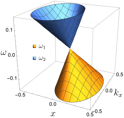
Figure 11: The tilted phase space Dirac cone of $H_{2}(x,k_{x},k_{y},k_{z})$ at the LC Weyl point. It faithfully represents the tilted Dirac cone of $H(x,k_{x},k_{y},k_{z})$ shown in Fig. 2.

For $H_{2}(x,k_{x},k_{y},k_{z})$, the corresponding PDO is

$$\hat{H}_{2}(x,k_{x},k_{y},k_{z})=\begin{pmatrix}\omega_{\text{pc}}-\beta x&\dfrac{\mathrm{i}}{\sqrt{2}\alpha}(\eta\partial_{x}-k_{y})\\[10.0pt] \dfrac{\mathrm{i}}{\sqrt{2}\alpha}(\eta\partial_{x}+k_{y})&\omega_{\text{pc}}+\dfrac{4\omega_{\text{pc}}}{\alpha^{2}}\beta x\end{pmatrix}.$$ (62)

The theorems proved in Sec. V shows that the full system $\hat{H}(x,-\mathrm{i}\eta\partial_{x},k_{y},k_{z})$ admits one topological edge mode, i.e., the TLCW, as confirmed by numerical solutions in Secs. II and III. This property of the TLCW is also faithfully captured by the reduced system $\hat{H}_{2}(x,k_{x},k_{y},k_{z})$.

In particular, Theorem 16 applies to $\hat{H}_{2}(x,k_{x},k_{y},k_{z})$ as well. From Eqs. (56) and (57), the common gap condition is satisfied for $\omega_{1}$ and $\omega_{2}$, and the proof of Theorem 16 shows that the Chern number $n_{c}\left(E_{1}\rightarrow S_{1}^{2}\right)$ of the first eigenmode bundle of $H_{2}(x,k_{x},k_{y},k_{z})$ over $S_{1}^{2}$ equals $1.$ Thus, $\hat{H}_{2}(x,k_{x},k_{y},k_{z})$ admits one spectral flow, i.e., the TLCW.

To thoroughly understand the physics of a tilted phase space Dirac cone and the TLCW, we present here the analytical solution of the entire spectrum of $\hat{H}_{2}(x,k_{x},k_{y},k_{z})$, including its spectral flow in the band gap. For the PDO corresponding to a $2\times 2$ symbol of a straight Dirac cone, its analytical solution has been given by Faure [2]. But for the PDO corresponding to a $2\times 2$ symbol of a tilted Dirac cone, we are not aware of any previous analytical solution.

To analytically solve for its spectrum, we first simplify the matrix $\hat{H}_{2}(x,k_{x},k_{y},k_{z})$ in Eq. (62). Subtract the entire spectrum by $\omega_{\mathrm{pc}}$ and renormalize $x$ and $k_{y}$ as follows,

$$\tilde{x}:=\sqrt{\dfrac{\sqrt{2}\alpha\beta\kappa}{\eta}}x,\quad\tilde{k}_{y}:=\dfrac{k_{y}}{\sqrt{\sqrt{2}\alpha\beta\eta\kappa}},$$ (63)

where $\kappa^{2}=4\omega_{\mathrm{pc}}/\alpha^{2}$. Matrix $\hat{H}_{2}$ in Eq. (62) then simplifies to

$$\hat{H}_{2}=\sqrt{\dfrac{\sqrt{2}\beta\eta\kappa}{\alpha}}\dfrac{1}{\sqrt{2}}\begin{pmatrix}-\tilde{x}/\kappa&\mathrm{i}(\partial_{\tilde{x}}-\tilde{k}_{y})\\ \mathrm{i}(\partial_{\tilde{x}}+\tilde{k}_{y})&\kappa\tilde{x}\end{pmatrix}.$$ (64)

It is clear that $\kappa$ is a parameter measuring how tilted the Dirac cone is. When $\kappa=1$, the Dirac cone is straight.

From now on in this section, the overscript tilde in $\tilde{x}$ and $\tilde{k}_{y}$ will be omitted for simple notation. We further transform $\hat{H}_{2}$ by a similarity transformation and scaling,

$$\hat{H}_{2}^{\prime} =\sqrt{\dfrac{\alpha}{\sqrt{2}\beta\eta\kappa}}R\hat{H}_{2}R^{-1}=\dfrac{1}{\sqrt{2}}\begin{pmatrix}-x/\kappa&\mathrm{i}(\partial_{x}-k_{y})/\kappa\\ \mathrm{i}\kappa(\partial_{x}+k_{y})&\kappa x\end{pmatrix},$$ (65)

$$R =\mathrm{diag}(\kappa,1).$$ (66)

$\hat{H}_{2}^{\prime}$ can be expressed using Pauli matrices and the identity matrix $\sigma_{0}$ as

$$\sqrt{2}\hat{H}_{2}^{\prime} =\mathrm{i}(\mu_{2}k_{y}+\mu_{1}\partial_{x})\sigma_{x}+(\mu_{1}k_{y}+\mu_{2}\partial_{x})\sigma_{y}-\mu_{1}x\sigma_{z}+\mu_{2}x\sigma_{0},$$ (67)

$$\mu_{1} =\dfrac{1}{2}\left(\kappa+\dfrac{1}{\kappa}\right),\quad\mu_{2}=\dfrac{1}{2}\left(\kappa-\dfrac{1}{\kappa}\right).$$ (68)

We next apply a unitary transformation to cyclically rotate Pauli matrices such that $(\sigma_{x},\sigma_{y},\sigma_{z},\sigma_{0})\to(\sigma_{y},\sigma_{z},\sigma_{x},\sigma_{0})$. Under this rotation, $\hat{H}_{2}^{\prime}$ becomes

$$\hat{H}_{2}^{\prime\prime}=\begin{pmatrix}\mu_{1}\lambda+\mu_{2}\hat{a}&\mu_{2}\lambda-\mu_{1}\hat{a}^{\dagger}\\ -\mu_{2}\lambda-\mu_{1}\hat{a}&-\mu_{1}\lambda+\mu_{2}\hat{a}^{\dagger}\end{pmatrix},$$ (69)

where $\lambda=k_{y}/\sqrt{2}$ and

$$\hat{a}=\dfrac{1}{\sqrt{2}}(x+\partial_{x}),\quad\hat{a}^{\dagger}=\dfrac{1}{\sqrt{2}}(x-\partial_{x}).$$ (70)

are annihilation and creation operators. Notice that $\mu_{1}=1$ and $\mu_{2}=0$ when $\kappa=1$, and this is the special case when $\hat{H}_{2}^{\prime\prime}$ reduces to a Hamiltonian corresponding to a straight Dirac cone [2, 30]. We now construct an analytical solution of $\hat{H}_{2}^{\prime\prime}$.

Recall that the eigenstates of a quantum harmonic oscillator $|n\rangle$ can be represented by the Hermite polynomials $H_{n}(x)$ as

$$\langle x|n\rangle=\varphi_{n}(x)=\frac{1}{\left(2^{n}n!\sqrt{\pi}\right)^{1/2}}\mathrm{e}^{-\frac{x^{2}}{2}}H_{n}(x).$$ (71)

Define a set of shifted wave functions $|n;\delta\rangle$ by

$$\langle x|n;\delta\rangle:=\varphi_{n}(x+\sqrt{2}\delta).$$ (72)

They satisfy the following iteration relations,

$$\hat{a}^{\dagger}|n;\delta\rangle =\sqrt{n+1}|n+1;\delta\rangle-\delta|n;\delta\rangle,$$ (73)

$$\hat{a}|n;\delta\rangle =\sqrt{n}|n-1;\delta\rangle-\delta|n;\delta\rangle.$$ (74)

With these shifted wave functions as basis, it can be verified that $\hat{H}_{2}^{\prime\prime}$ has two sets of eigenvectors,

$$\psi_{n}^{\pm}=\begin{pmatrix}|n+1;\delta_{n}^{\pm}\rangle\\ \gamma_{n}^{\pm}|n;\delta_{n}^{\pm}\rangle\end{pmatrix},\quad n=0,1,2,\cdots\thinspace,$$ (75)

where

$$\gamma_{n}^{\pm}=\dfrac{\sqrt{n+1}}{-\lambda\mp\sqrt{\lambda^{2}+n+1}},\quad\delta_{n}^{\pm}=\pm\dfrac{\mu_{2}}{\mu_{1}}\sqrt{\lambda^{2}+n+1}.$$

The corresponding eigenvalues are

$$E_{n}^{\pm}=\pm\dfrac{2\kappa}{1+\kappa^{2}}\sqrt{\lambda^{2}+n+1},\quad n=0,1,2,\cdots\thinspace.$$ (76)

Importantly, there is one additional eigenstate that is not included in Eq. (75), which, in fact, represents the spectrum flow. Its eigenvector and eigenvalue are

$$\psi_{-1}=\begin{pmatrix}|0;\delta_{-1}\rangle\\ 0\end{pmatrix},\quad E_{-1}=\dfrac{2\kappa}{1+\kappa^{2}}\lambda,$$ (77)

where

$$\delta_{-1}=\dfrac{\mu_{2}}{\mu_{1}}\lambda.$$ (78)

Here, we abusively denote this eigenmode as the “$n=-1$” eigenstate. The spectral flow is a linear function of $k_{y}$, and its mode structure is a shifted Gaussian function.

The spectrum of $\hat{H}_{2}^{\prime\prime}(x,-\mathrm{i}\partial_{x},\lambda)$ are plotted in Fig. 12(a). The spectrum consists of three parts, the upper and lower parts are the global modes in the frequency bands of $H_{2}(x,k_{x},k_{y},k_{z})$. The middle part is the single spectral flow connecting the left of the lower part to the right of the upper part. Note that the tilted Dirac cone of $H_{2}(x,k_{x},k_{y},k_{z})$ breaks up into two pieces in the global modes of $\hat{H}_{2}^{\prime\prime}(x,-\mathrm{i}\partial_{x},\lambda)$. In Fig. 12(b), the analytical solution of the mode structure of the spectral flow of $\hat{H}_{2}^{\prime\prime}(x,-\mathrm{i}\partial_{x},\lambda)$ is plotted. The analytical result displayed in Fig. 12 agrees well with the numerical solution shown in Fig. 4.

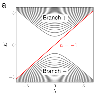
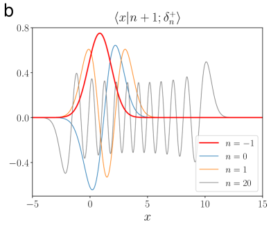
Figure 12: (a) Analytical spectrum of $\hat{H}_{2}^{\prime\prime}(x,-\mathrm{i}\partial_{x},\lambda)$ as a function of $k_{y}$. (b) Analytical mode structure of the TLCW. The result agrees well with the numerical solution shown in Fig. 4.

VII Conclusions and discussions

Inspired by advances in topological materials in condensed matter physics [31, 32, 33, 34, 35, 36], study of topological waves in classical continuous media, such as electromagnetic materials [8, 9, 10, 11], fluid systems [1, 2, 12, 13, 14, 15, 16, 17, 18, 19], and magnetized plasmas [20, 21, 22, 4, 23, 5, 6, 24, 25], has attracted much attention recently. The Topological Langmuir-Cyclotron Wave (TLCW) is a recently identified topological surface excitation in magnetized plasmas generated by the nontrivial topology at the Weyl point due to the Langmuir wave-cyclotron wave resonance [5, 6]. In this paper, we have systematically developed a theoretical framework to describe the TLCW.

It has been realized that the theoretical methodology for studying topological material properties in condensed matter physics cannot be directly applied to classical continuous media, because the momentum (wavenumber) space for condensed matter is periodic, whereas that for classical continuous media is not. Specifically, the typical momentum space for classical continuous media is $\mathbb{R}^{n}$ $(n=1,2,3),$ and it is difficult to integrate the Berry curvature over $\mathbb{R}^{n}$ to obtain an integer number that can be called the Chern number. The difficulty has been attributed to the fact that $\mathbb{R}^{n}$ is not compact, and different remedies have been proposed accordingly. However, we demonstrated that the key issue is not whether the momentum space is non-compact, but rather that it is contractible. When the base manifold is contractible, all vector bundles on it are topologically trivial, and whether an integer index can be designed is irrelevant. For classical continuous media, nontrivial topology can be found only for vector bundles over phase space. Without modification, the Atiyah-Patodi-Singer (APS) index theorem [7] proved for spectral flows over $S^{1}$ is only applicable to condensed matters, and Faure’s index theorem [2] for spectral flows over $\mathbb{R}$-valued $k_{y}$ should be adopted for classical continuous media.

In the present study, the TLCW is defined as a spectral flow of a Pseudo-Differential-Operator (PDO) $\hat{H}$ for plasma waves in an inhomogeneous magnetized plasma, and the semi-classical parameter of the Weyl quantization operator is identified as the ratio between electron gyro-radius and the scale length of the inhomogeneity. We formally constructed the Hermitian eigenmode bundles of the bulk Hamiltonian symbol $H$ corresponding to the PDO $\hat{H},$ and emphasized that the properties of spectral flows are determined by the topology of the eigenmode bundles over non-contractible phase space manifolds. To calculate Chern numbers of eigenmode bundles over a 2D sphere in phase space, as required by Faure’s index theorem, a boundary isomorphism theorem (Theorem 12) was established.

The TLCW is proved to exist in magnetized plasmas as a spectral flow with the spectral index being one. The Chern theorem (Theorem 6), instead of the Berry connection or any other connection, was used to calculate the Chern numbers. Finally, we developed an analytically solvable model for the TLCW using a tilted phase space Dirac cone. An analytical solution of the PDO of a generic tilted phase space Dirac cone was found, which generalized the previous result for a straight Dirac cone [2]. The spectral flow index of the tilted Dirac cone was calculated to be one, and the mode structure of the spectral flow was found to be a shifted Gaussian function.

As a topological edge wave, the TLCW can propagate unidirectionally and without reflection and scattering along complex boundaries. Due to this topological robustness, it might be relatively easy to excite the TLCW experimentally. Of course, laboratory and astrophysical plasmas are subject to many more physical effects that have not been included in the present model, such as collisions and finite temperature. For practical application, these factors need to be carefully evaluated by experimental and theoretical methods.